Deep-Learning-Aided Distributed Clock Synchronization for Wireless Networks

Abstract

The proliferation of wireless communications networks over the past decades, combined with the scarcity of the wireless spectrum, have motivated a significant effort towards increasing the throughput of wireless networks. One of the major factors which limits the throughput in wireless communications networks is the accuracy of the time synchronization between the nodes in the network, as a higher throughput requires higher synchronization accuracy. Existing time synchronization schemes, and particularly, methods based on pulse-coupled oscillators (PCOs), which are the focus of the current work, have the advantage of simple implementation and achieve high accuracy when the nodes are closely located, yet tend to achieve poor synchronization performance for distant nodes. In this study, we propose a robust PCO-based time synchronization algorithm which retains the simple structure of existing approaches while operating reliably and converging quickly for both distant and closely located nodes. This is achieved by augmenting PCO-based synchronization with deep learning tools that are trainable in a distributed manner, thus allowing the nodes to train their neural network component of the synchronization algorithm without requiring additional exchange of information or central coordination. The numerical results show that our proposed deep learning-aided scheme is notably robust to propagation delays resulting from deployments over large areas, and to relative clock frequency offsets. It is also shown that the proposed approach rapidly attains full (i.e., clock frequency and phase) synchronization for all nodes in the wireless network, while the classic model-based implementation does not.

I Introduction

Time synchronization stands as a primary precondition for many applications, making it a broad and crucial field of research. In particular, time synchronization is critical for the successful operation of wireless communications networks relying on time division multiple access (TDMA) to facilitate resource sharing. With TDMA, each connected device in the network is allocated a dedicated time slot for transmission. Therefore, time synchronization among the devices is essential to ensure that there are no collisions, facilitating spectral efficiency maximization [1, 2]. One example for the importance of clock synchronization in TDMA-based networks is the deployment of wireless sensor networks in hazardous and/or secluded environments: In such scenarios, it may be impractical to recharge or replace the battery at the sensor nodes [3]. To save power, an accurately synchronized TDMA scheme can be applied to WSNs such that the nodes are in sleep mode except during the TDMA slots in which they transmit [4], [5].

Synchronization can be achieved via various approaches, which can be classified as either local synchronization (involving the use of clustered nodes) or global synchronization (where all nodes are synchronized to a global clock). In the context of ad-hoc wireless networks, it is typically preferable for the nodes to synchronize in a distributed manner, such that the nodes in the network obtain and maintain the same network clock time independently, without requiring direct communications with a global synchronization device [6]. Thus, distributed synchronization is more robust to jamming, and can be applied in scenarios in which commonly used global clocks, such as the Global Positioning System (GPS), are unavailable, e.g., in underground setups. Traditional distributed time synchronization algorithms require periodic transmission and reception of time information, which is commonly implemented via packets containing a time-stamp data, exchanged between the coupled nodes [7]. Packet-based synchronization has been broadly studied for wired and wireless network, [8], with proposed protocols including the flooding time synchronization protocol [9], Precision Time Protocol [10], Network Time Protocol [11], generalized Precision Time Protocol [12], and Precision Transparent Clock Protocol [13, Sec. 3.5]. These approaches differ in the the way the time-stamp information is encoded, conveyed and processed across the nodes. The major drawbacks of packet-based coupling are the inherent unknown delays in packet formation, queuing at the MAC layer, and packet processing at the receiver. These delays could potentially make the received time stamp carried by the packet outdated after processing is completed. Another significant drawback is the high energy consumption due to the associated processing [6].

An alternative approach to packet-based synchronization, which offers lower energy consumption and simpler processing, is to utilize the broadcasting nature of the wireless medium for synchronization at the physical-layer. In this approach, the time information corresponds to the time at which the waveform transmitted by a node is received at each of the other nodes, hence, avoiding the inherently complex processing of the packet at the MAC layer and at the receiver [6]. One major approach for physical-layer synchronization is based on pulse-coupled oscillators, which use the reception times of the pulses transmitted by the other nodes to compute a correction signal applied to adjust the current node’s voltage controlled clock (VCC) [6, 14, 15]. In classic PCO-based synchronization [6], the correction signal is based on the output of a phase discriminator (PD) which computes the differences between the node’s own time and the reception times of the pulses from the other nodes. These differences are weighted according to the relative received pulse power w.r.t the sum of the powers of the pulses received from the other nodes. While with this intuitive weighting PCO-based synchronization is very attractive for wireless networks, the resulting synchronization performance significantly degrade in network configurations in which there are large propagation delays and clock frequency differences, and generally, full clock synchronization (frequency and phase) is not attained by current PCO-based schemes, see, e.g., [6]. This motivates the design of a robust PCO-based time synchronization scheme, which is the focus of the current work.

Main Contributions: In this work we propose a PCO-based time synchronization scheme which is robust to propagation delays. To cope with the inherent challenge of mapping the output of the PD into a VCC correction signal, we use a DNN, building upon the ability of neural networks to learn complex mappings from data. To preserve the energy efficiency and distributed operation of PCO-based synchronization, we employ the model-based deep learning methodology [16, 17, 18]. Accordingly, our algorithm, coined -aided synchronization algorithm (DASA), augments the classic clock update rule of [6, Eqn. (16)] via a dedicated DNN. In particular, we design DASA based on the observation that conventional PCO-based synchronization is based on weighted averaging of the outputs of the PD, which can be viewed as a form of self-attention mapping [19]. Thus, DASA utilizes attention pooling, resulting in a trainable extension of the conventional algorithm. To train our model in a distributed fashion, we formulate a decentralized loss measure designed to facilitate rapid convergence, which can be computed at each node locally, resulting in a decentralized fast time synchronization algorithm. Our numerical results clearly demonstrate that the proposed DASA yields rapid and accurate synchronization in various propagation environments, outperforming existing approaches in both convergence speed and performance. The proposed scheme is also very robust to values of the clock frequencies and to nodes’ locations.

Organization: The rest of this work is organised as follows: Section II reviews the fundamental structure of PCO-based synchronization schemes. Section III presents the problem formulation, highlights the weaknesses of the classic weighting rule and states the objective of this work. Subsequently, Section IV presents our proposed DASA. Numerical examples and discussions are provided in Section V. Lastly, Section VI concludes this work.

Notations: In this paper, deterministic column vectors are denoted with boldface lowercase letters, e.g., $\mathbf{x}$, deterministic scalars are denoted via standard lowercase fonts, e.g., $x$, and sets are denoted with calligraphic letters, e.g., $\mathcal{X}$. Uppercase Sans-Serif fonts represent matrices, e.g., $\mathsf{K}$, and the element at the $i$’th row and the $j$’th column of $\mathsf{K}$ is denoted with $\mathsf{K}_{i,j}$. The identity matrix is denoted by $\mathsf{I}$. The sets of positive integers and of integers are denoted by $\mathcal{N}$ and $\mathcal{Z}$, respectively. Lastly, all logarithms are taken to base-2.

II Distributed Pulse-Coupled Time Synchronization for Wireless Networks

II-A Network and Clock Models

We study discrete-time (DT) clock synchronization for wireless networks, considering a network with $N$ nodes, indexed by $i\in\{1,2,...,N\}\triangleq\mathcal{I}_{N}$. Each node has a clock oscillator with its own inherent period, denoted by $T_{i}$, $i\in\mathcal{I}_{N}$. Generally, clock timing is often affected by an inherent random jitter, also referred to as phase noise. Let $V_{i}(k)$ denote the phase noise at node $i\in\mathcal{I}_{N}$, at time index $k\in\mathcal{Z}$. Then, the corresponding clock time $\phi_{i}(k)$, can be expressed with respect to $k=0$ as

$$\phi_{i}(k)=\phi_{i}(0)+k\cdot T_{i}+V_{i}(k).$$ (1)

In this work we assume $V_{i}(k)=0$, $\forall k\in\mathcal{Z}$ (see, e.g., [20, Sec.V], [6]) in order to focus on the fundamental factors affecting synchronization performance in wireless networks, which are the propagation delays and clock period differences.

In a wireless network, when the clock periods of the different nodes, $T_{i}$, $i\in\mathcal{I}_{N}$, are different, then the nodes’ transmissions may overlap in time and frequency (a situation which is referred to as “collision”), resulting in loss of information. Moreover, even when the clock periods are identical, referred to as clock frequency synchronization, a time offset (also referred to as phase offset) between the clocks may exist, which again will result in collisions, as illustrated in Fig. 1. Thus, to facilitate high speed communications, the nodes must synchronize both their clock frequencies as well as their clock phases to a common time base. This is referred to as full clock synchronization. To that aim, the nodes in the network exchange their current time stamps, and, based on the exchanged time information, the nodes attempt to reach a consensus on a common clock.

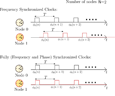
Figure 1: An illustration of clock frequency synchronization and of full clock synchronization, for a network which consists of two nodes.

A wireless communications setup can be represented via a connectivity graph $\mathcal{X}$, consisting of a vertex set representing the nodes, and an edge set representing the links [21, Ch. 1]. The edges between pairs of vertices (i.e., pair of nodes) are weighted by an adjacency matrix $\mathsf{A}$, whose $(i,j)$’th entry, $\left[\mathsf{A}\right]_{i,j}$, satisfies $\left[\mathsf{A}\right]_{i,j}\geq 0$, where $\left[\mathsf{A}\right]_{i,j}=0$ implies that there is no direct link between nodes $i$ and $j$. A connectivity graph has girth that is larger than one, hence the diagonal entries of $\mathsf{A}$ are zero (i.e., $\left[\mathsf{A}\right]_{i,i}=0$). In the next subsections we recall results on the convergence of PCO-based synchronization algorithms, obtained using the adjacency graph formulation, for specific cases discussed in the literature.

Lastly, we note that in this work it is assumed that node locations are static and the propagation channels are time-invariant. The case of time-varying communications links has been studied in [22, 23, 24], for which the adjacency matrix $\mathsf{A}$ randomly evolves over time, and each node subsequently updates its coefficients following the information received from the other nodes. In [22], necessary conditions for convergence were established by combining graph theory and system theory for bidirectional and for unidirectional links. It was concluded in [22] that synchronization could fail, even for fully-connected networks.

II-B Pulse-Coupled PLLs

As stated earlier, physical layer synchronization techniques operate by conveying the timing information of the nodes across to neighboring nodes via transmitted waveforms. Specifically, each node $i\in\mathcal{I}_{N}$ broadcasts a sequence of synchronization signatures, which uniquely identifies the transmitting node, as in, e.g., [25], where transmission times are determined at each transmitting node according to its own local clock. Each receiving node then processes the synchronization signatures received from all the other nodes, and updates its local clock using to a predetermined update rule.

The distributed pulse-coupled phase locked loop (PLL) configuration is depicted in Fig. 2. It is assumed that the nodes operation is full-duplex, i.e., the nodes can transmit and receive at the same time. At each node, the synchronization mechanism is based on a loop, which consists of a phase difference detector (PDD), a linear, time-invariant (LTI) filter with a transfer function $\varepsilon(z)$, and a VCC. Each node is fed with the measured reception times of the pulses received from the different nodes, which are input to the PDD. The PDD calculates the difference between the time of each received pulse and the node’s own clock, and weights this difference with an a-priori computed weighting factor, which is associated to the appropriate node based on its synchronization signature. The PDD outputs the sum of the weighted differences to the loop filter $\varepsilon(z)$, which generates a correction signal for the VCC.

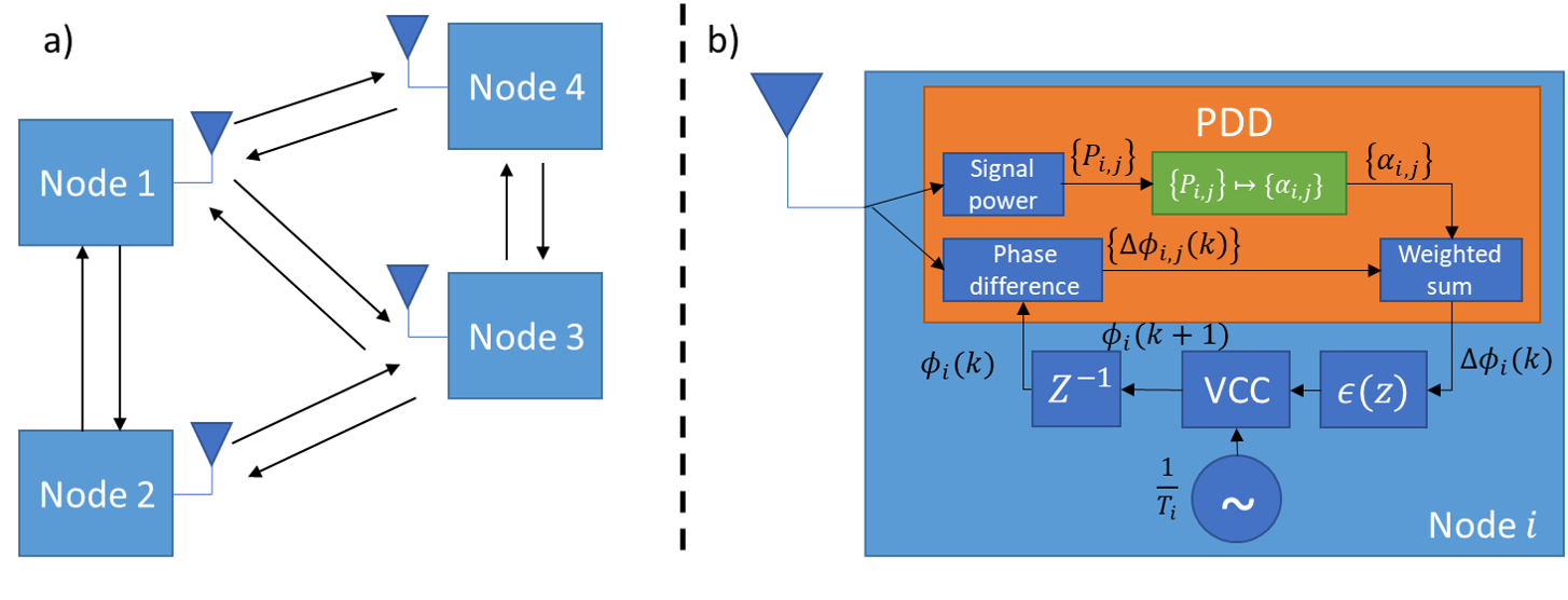
Figure 2: Diagram showing (a) sample topological deployment of $N=4$ pulse-coupled nodes; (b) the structure of the synchronization mechanism based on the classical model (4), see [6].

Mathematically, the output of the PDD at time index $k\in\mathcal{N}$, at the $i$’th node, denoted by $\Delta\phi_{i}(k)$, can be expressed as:

$$\Delta\phi_{i}(k)=\mathop{\sum}\limits_{j=1,j\neq i}^{N}\alpha_{i,j}\cdot\left(t_{i,j}(k)-\phi_{i}\left(k\right)\right),$$ (2)

where $\alpha_{i,j}\in[0,1]$, and $t_{i,j}(k)\triangleq\phi_{j}\left(k\right)+q_{i,j}(k)$ is the reception time at node $i$ of the pulse transmitted by node $j$; which corresponds to the sum of the transmission time, $\phi_{j}\left(k\right)$, and the propagation delay $q_{i,j}(k)$ from node $j$ to node $i$. The PDD output is then fed into a loop filter $\varepsilon(z)$ whose output drives the VCC that re-calibrates the instantaneous time at the $i$’th node.

II-C The Classic Pulse-Coupled PLL Configuration

For the classic PCO-base PLL design of [6], the $(i,j)$’th entry of the adjacency matrix $\mathsf{A}$ corresponds to the relative signal power of the pulse received at node $i$ from node $j$, with respect to the powers of all the other nodes received at node $i$: Denoting $\left[\mathsf{A}\right]_{i,j}=\alpha_{i,j}$ and letting $P_{i,j}$ denote the power of the pulse received at node $i$ from node $j$, then, in the classic algorithm of [6], $\alpha_{i,j}$ is computed as [26, 6, 27]:

$$\alpha_{i,j}=\frac{P_{i,j}}{\mathop{\sum}\limits_{j=1,j\neq i}^{N}P_{i,j}}.$$ (3)

From Eqn. (3) it follows that the value of $\alpha_{i,j}$ depends on the distance between the nodes as well as on other factors which affect the received power levels, e.g., shadowing and fading. When implementing a first-order PLL, then $\varepsilon(z)$ is set to $\varepsilon(z)=\varepsilon_{0}$, and letting $\Delta\phi_{i,j}(k)\triangleq\phi_{j}\left(k\right)+q_{i,j}(k)-\phi_{i}\left(k\right)$, the update rule is (see [6, Eqns. (16), (23)]):

$$\phi_{i}\left(k+1\right)=\phi_{i}(k)+T_{i}+\varepsilon_{0}\cdot\mathop{\sum}\limits_{j=1,j\neq i}^{N}\alpha_{i,j}\cdot\Delta\phi_{i,j}(k).$$ (4)

We refer to the rule (4) with weights (3) as the classic algorithm or the analytic algorithm.

In this work, we investigate distributed synchronization based on DT pulse-coupled PLL. With the adjacency matrix $\mathsf{A}$ defined above, the Laplacian matrix of the connectivity graph $\mathcal{X}$ is given as $\mathsf{L}=\mathsf{I}-\mathsf{A}$. It has been noted in [6] that for pulse-coupled first-order DT PLLs, synchronization can be achieved if and only if $|\lambda_{l}(\mathsf{L})|>0,\forall 2\leq l\leq N$, where $\lambda_{l}(\mathsf{L})$ denotes the $l$’th eigenvalue of the matrix $\mathsf{L}$, arranged in ascending order. In general, when using pulse-coupled PLLs, synchronization across the nodes is attained when the connectivity graph is strongly connected; in other words, there should be a path connecting any node pair. The connection between each pair need not be direct, may also run via intermediate nodes, as long as all nodes in the network are able to exchange timing information among each other [28]. Hence, if there exists at least one node whose transmissions can be received at all the nodes in the network (directly or via intermediate nodes), then, clock frequency synchronization can be achieved.

The rule in (4) was expressed as a time-invariant difference equation in [6], for which the steady-state phase expressions for the nodes, in the limit as $k$ increases to infinity were derived. Specifically, for the case of no propagation delay and identical clock periods at all nodes, i.e., $q_{i,j}(k)=0$, $i,j\in\mathcal{I}_{N}$, $k\in\mathcal{Z}$, and $T_{i}=T_{\mbox{\scriptsize nom}}$, $i\in\mathcal{I}_{N}$, the rule (4) generally results in the network attaining full synchronization. On another hand, when there are propagation delays and/or different clock periods at the nodes, then typically, frequency synchronization to a common frequency is attained, but full synchronization is not attained. We consider in this paper the common and more practical scenario where there are propagation delays and different clock periods, which generally results in asynchronous clocks at steady state. Accordingly, the objective of our algorithm is to attain full synchronization for this important scenario.

III Problem Formulation

Consider a network with $N$ nodes, such that each node $i\in\mathcal{I}_{N}$ has its own clock with an inherent period of $T_{i}$, where generally $T_{i}\neq T_{j}$ for $i\neq j$, and let $\phi_{i}(k)$ be the clock time at DT time index $k\in\mathcal{N}$. The nodes are located at geographically separate locations, where node $i$ is located at coordinate $(x_{i},y_{i})$, and $d_{i,j}$ is the distance between nodes $i$ and $j$. Assuming line-of-sight propagation, a signal transmitted from node $i$ is received at node $j$ after $q_{i,j}=\frac{d_{i,j}}{c}$ seconds, where $c$ is the speed of light. We assume that the nodes are not aware of their relative locations and of the clock periods at the other nodes. The objective is to synchronize the clock times $\{\phi_{i}(k)\}_{i\in\mathcal{I}_{N}}$ such that at steady-state, at each $k$, it holds that $\phi_{i}(k)=\phi_{j}(k)$, $\forall i\neq j$.

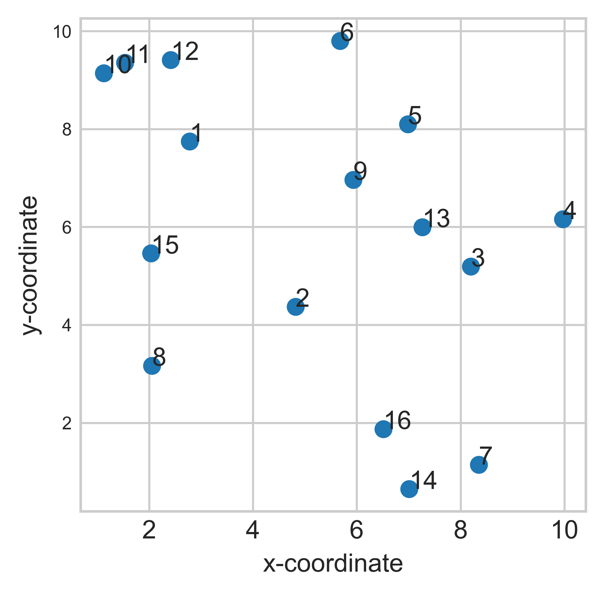
(a)

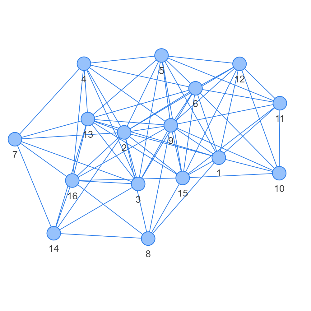
(b)

Figure 3: (a) Geographic locations of the nodes in the wireless network considered in Section III and (b) Network graph showing the connected node pairs.

To motivate the proposed approach we first illustrate the weakness of the analytic update rule of [6, Eqns. (16), (23)]), as discussed in Section II-B. This rule has been acceptable as a baseline rule in multiple works on network clock synchronization, e.g., [29, 30, 31], hence, we use it as a baseline for the performance of our proposed algorithm. As a motivating scenario, consider a wireless network with $N=16$ nodes located in a square area of dimensions $10\;[\mbox{Km}]\times 10\;[\mbox{Km}]$, with locations depicted in Fig. 3. In this example, each node has a random clock time at startup [6], taken uniformly over $[0,T_{i}]$, see, e.g., [25, 29, 32, 33]. Each node transmits periodically at its corresponding clock times, and processes the pulse timing for its received pulses using the DT PLL update rule of [6, Eqns. (16), (23)] to synchronize their clocks, see Eqn. (4).

For the purpose of the numerical evaluation, we let the nominal period of the clocks in the network, denoted $T_{\mbox{\scriptsize nom}}$, be $T_{\mbox{\scriptsize nom}}=\frac{1}{200}\;[\mbox{sec}]$. The period $T_{i}$ for the VCC of node $i$ is obtained as by randomly generating clock periods with a maximum deviation of $100$ [ppm]:

$$T_{i}=T_{\mbox{\scriptsize nom}}\cdot(1+B_{0}\cdot 10^{-A}),$$ (5)

where $B_{0}$ is a uniformly distributed random variable whose value is either $1$ or $-1$, and $A$ is uniformly selected from the interval $[4,6]$. For time-invariant channels, the corresponding propagation delays are given by $q_{i,j}(k)=q_{j,i}(k)=\frac{d_{i,j}}{c}$, $\forall i,j\in\mathcal{I}_{N}$ and $k\in\mathcal{N}$.

For simplicity we assume identical transmit power of $P_{t}=33$ [dBm] at all nodes (different powers can be modeled using different topologies), and a two-ray wireless propagation model, in which the received signal consists of a direct line-of-sight component and a single ground reflected wave component. Assuming isotropic antennas, the antenna gains are is $G_{i}=1$ at all directions, $\forall i\in\mathcal{I}_{N}$. For node heights of $1.5$ [m], it follows that the received power at node $i$ from node $j$, denoted $P_{i,j}$, is given by the expression: [34, Eqn. 2.1-8]:

$$P_{i,j}\approx\frac{P_{t}\cdot G_{j}G_{i}h_{i}^{2}h_{j}^{2}}{\left(d_{i,j}\right)^{4}}=\frac{10}{\left(d_{i,j}\right)^{4}}=P_{j,i}.$$ (6)

We assume receiver sensitivity of $-114$ [dBm], [35], [36], [37] and as a result, $48$ node pairs do not have direct reception. This is depicted in the graph in Fig. 3(b), in which nodes not connected by edges do not have a direct link. The evaluated received power levels are then applied in calculation of the weights $\alpha_{i,j}$ via Eqn. (3).

In Figs. 4 and 5 we evaluated the performance of the rule [6, Eqns. (16), (23)] for a first-order PLL with $\varepsilon(z)=1$ and for a second-order PLL with $\varepsilon(z)=\frac{1}{1-0.3z^{-1}}$, respectively. Figs. 4(a) and 5(a) depict the evolution of the clock periods for all the nodes, for the first-order PLL and the second-order PLL, respectively, as $k$ increases: The period is observed to converge to a mean value at time $k=2799$, $T_{c,ANA}(2799)=0.00500208$, and $T_{c,ANA_{1}}(2799)=0.00500274$, respectively, which indeed demonstrates that frequency synchronization is achieved. The evolution of the modulus of the clock phases w.r.t the synchronized periods $T_{c,ANA}(2799)$ and $T_{c,ANA_{1}}(2799)$ when $\varepsilon(z)$ corresponds to a first-order PLL and to a second-order PLL, respectively, vs. $k$, is depicted in Figs. 4(b) and 5(b). Observe that indeed, for both PLLs, different phases are achieved at steady state. It follows that the algorithm [6, Eqns. (16), (23)] achieves frequency synchronization but not full synchronization, resulting in collisions between the transmissions of the different nodes, which, in turn, reduce the throughput of the communications network.

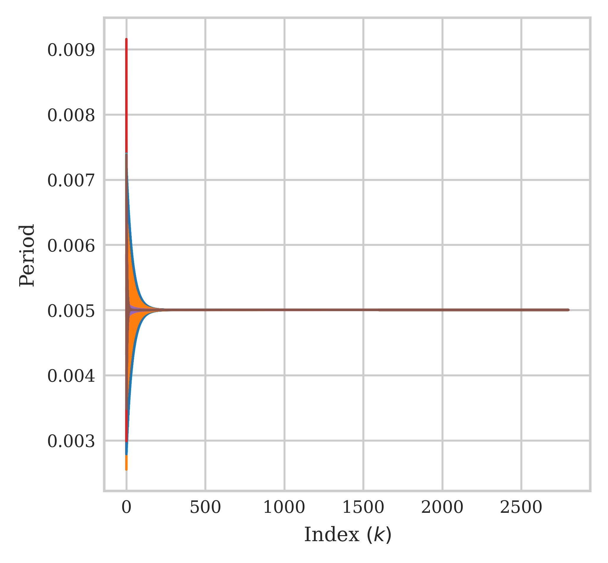
(a)

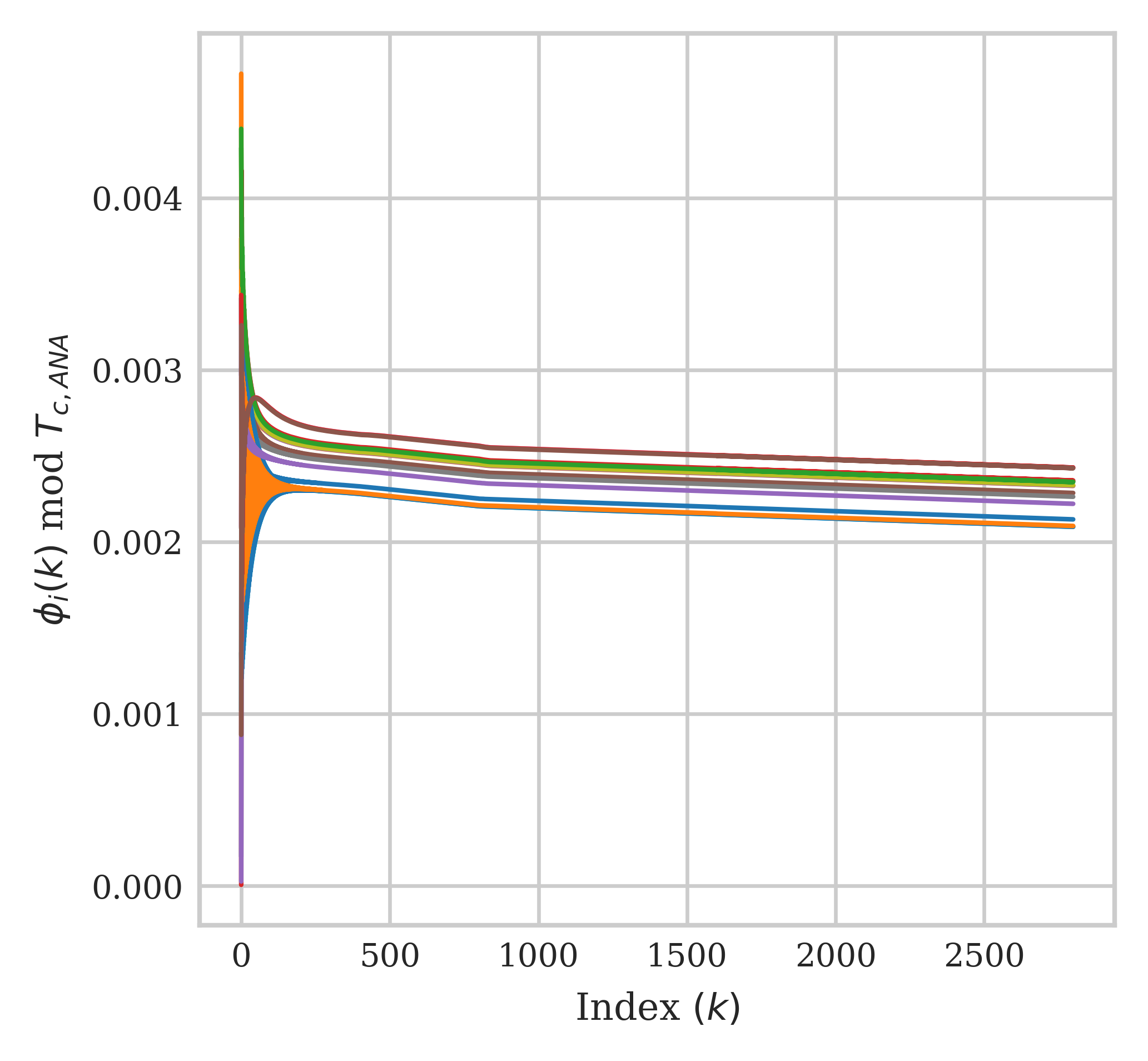
(b)

Figure 4: Simulation results for the analytical model defined in Eqn. (4) with a first-order PLL $\varepsilon(z)=1$ (a) The evolution of the clock periods for all $16$ nodes; (b) Clock times $\phi_{i}(k)$ modulo $T_{c,ANA}(2799)$, $i\in\mathcal{I}_{N}$, with fixed $\alpha_{i,j}$’s computed via Eqn. (3).

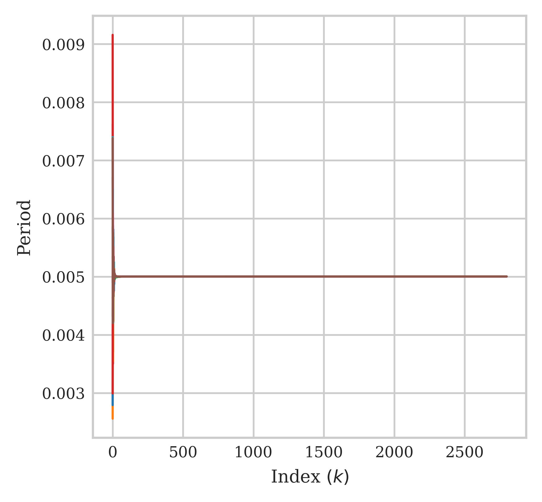
(a)

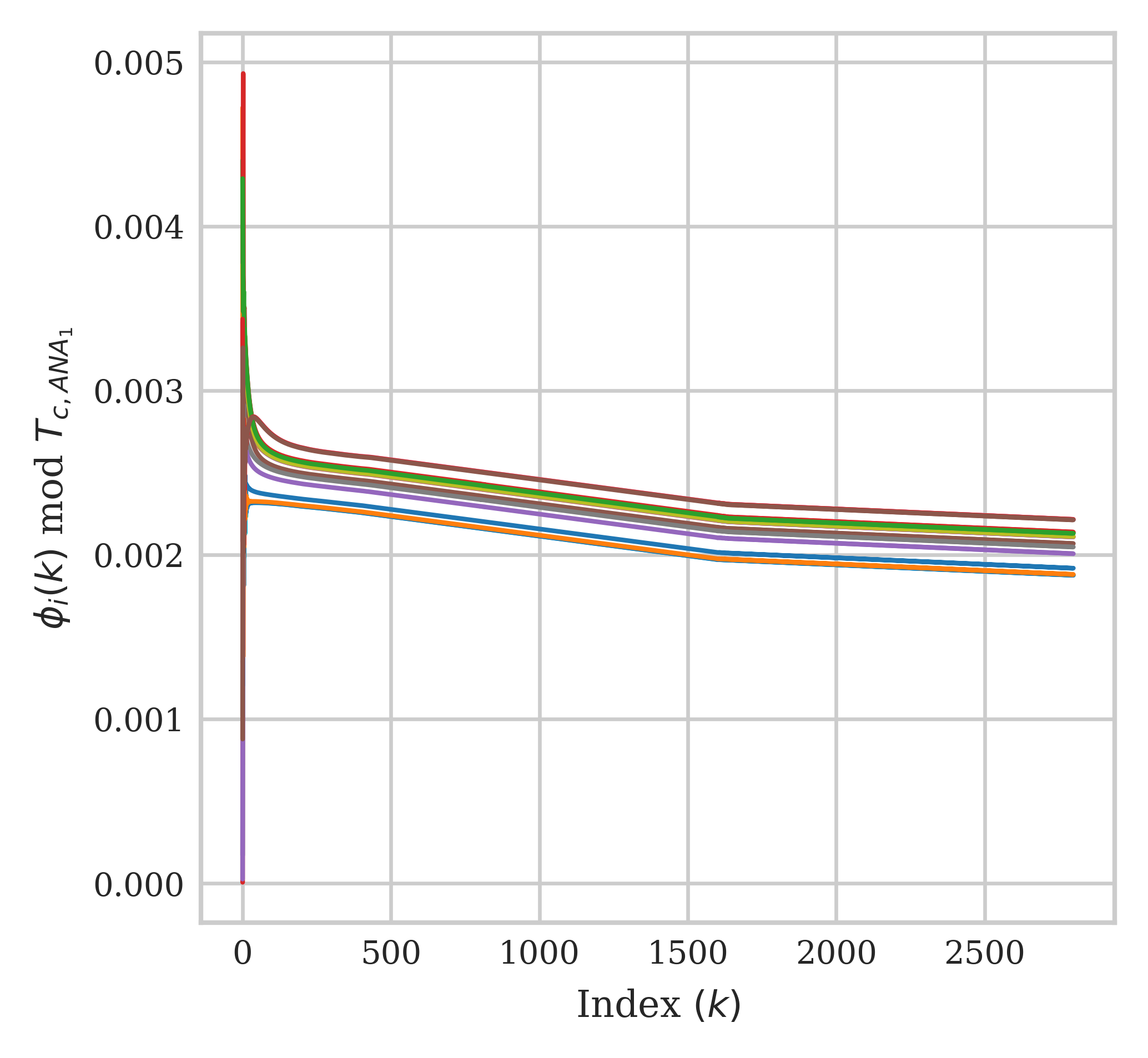
(b)

Figure 5: Simulation results for the analytical model defined in Eqn. (4) with a second order PLL $\varepsilon(z)=\frac{1}{1-0.3z^{-1}}$ (a) The evolution of the clock periods for all $16$ nodes; (b) Clock times $\phi_{i}(k)$ modulo $T_{c,ANA_{1}}(2799)$ $i\in\mathcal{I}_{N}$, with fixed $\alpha_{i,j}$’s computed via Eqn. (3)

.

The examples above illustrate the motivation for our proposed solution: As the ad-hoc analytic expression of the weights does not lead to satisfactory synchronization performance when propagation delays and/or clock period differences exist, we propose to use a DNN-aided mechanism to learn the VCC correction signals at the nodes, which lead to full network clock synchronization. In addition to attaining the desired performance, attention is also given to practicality of implementation. Therefore, we require that the algorithm will operate in a distributed manner, such that each node adapts its clock independently, processing only its own received signals. This is motivated by the fact that without independent processing, the network throughput is further decreased due to the exchange of messages for facilitating coordinated processing. As the update rule in Eqn. (4) achieves partial synchronization and is plausible from an engineering perspective, our approach maintains the structure of the update rule, replacing only the weights $\alpha_{i,j}$ with coefficients learned using a DNN, where the loss function used for training the DNN coefficients is calculated locally at each node. This approach, referred to as model-based learning, is motivated by the fact that the coefficients computation (3) does not account for clock frequency differences between the nodes and does not fully account for propagation delays, thus it is reasonable to expect a trained DNN to better account for these factors. Model-based learning is also shown to carry the important advantage of robustness to the training set, as the learned functionality is restricted and does not entail end-to-end operation [17, 16, 18]. In the next section we detail the proposed DNN-based clock synchronization algorithm.

IV DNN-Aided Distributed Clock Synchronization Algorithm

In this section we present the proposed DASA. We first describe the overall system in Section IV-A. Then, in Section IV-B we detail how DASA can be trained locally at each node in an unsupervised manner. We conclude with a discussion and a complexity analysis of the algorithm in Section IV-C.

IV-A Augmenting PLL-Based Synchronization with Deep Learning

Our proposed algorithm builds upon the classic PLL-based synchronization model, while augmenting its operation with a dedicated DNN, in order to learn the appropriate weights for scenarios with non-negligible propagation delays and with clock frequency offsets. Our design is inspired by attention mechanisms, which have demonstrated dramatic empirical success in natural language and in time sequence processing [19]. Attention mechanisms are deep models that learn to compute input-dependent weighting coefficients as a means of assigning increased significance to certain input sets and a lesser significance to others, which bears a clear similarity to the effect of the weighting coefficients $\{\alpha_{i,j}\}$ on the PDD output in (4). Consequently, we replace the model-based weighting via $\{\alpha_{i,j}\}$ in Eqn. (3) with a DNN-aided computation, where, again inspired by the success of self-attention mechanisms, we provide as inputs to the DNN not only the power levels (as needed by the classic algorithm, see Eqn. (3)) but also the relative time differences $\{\Delta\phi_{i,j}(k)\}$. The resulting algorithm, coined DASA, is schematically depicted in Fig. 6. DASA preserves the structure of the model-based DT PLL synchronization scheme fo Eqn. (4), while harnessing the capabilities of the DNN to learn abstract mappings from data, in order to replace the model-based weighting coefficients, which result in the classical algorithm being sensitive to propagation delays and clock frequency differences.

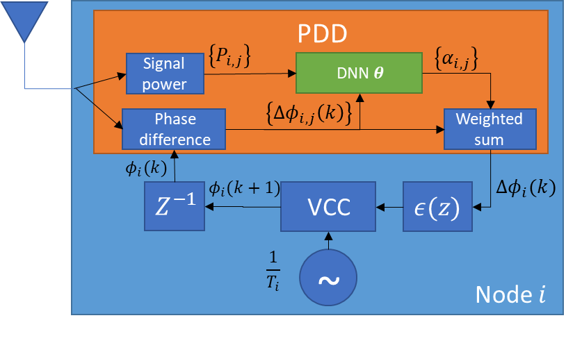
Figure 6: Block diagram of the proposed DASA.

We denote the DNN parameters at node $i$ by ${\boldsymbol{\theta}}_{i}(\cdot)$, and use $\psi_{{\boldsymbol{\theta}}_{i}}$ to denote the resulting mapping. For a given value of ${\boldsymbol{\theta}}_{i}$, the DNN at node $i$ maps the $2(N-1)$ values $\big{\{}\Delta\phi_{i,j}(k),P_{i,j}(k)\big{\}}_{j=1,j\neq i}^{N}$ into the $N-1$ weighting coefficients $\{\alpha_{i,j}\}$. Note that the coefficients $\{\alpha_{i,j}\}$ also vary with $k$. The weighted sum of $\Delta\phi_{i,j}(k)$ is then input to a loop filter with a transfer function $\varepsilon(z)$, and the output of the loop filter drives the VCC. The overall resulting time update rule can be expressed as

$$\phi_{i}\left(k+1\right)=\phi_{i}(k)+T_{i}+\varepsilon_{0}\cdot\mathop{\sum}\limits_{j=1,j\neq i}^{N}\Big{[}\psi_{{\boldsymbol{\theta}}_{i}}\Big{(}\Big{\{}\big{(}\Delta\phi_{i,j}(k),P_{i,j}(k)\big{)}\Big{\}}_{j=1,j\neq i}^{N}\Big{)}\Big{]}_{j}\cdot\Delta\phi_{i,j}(k),\vspace{-0.05cm}$$ (7)

where $\big{[}\psi_{{\boldsymbol{\theta}}_{i}}(\cdot)\big{]}_{j}$ denotes the output of the DNN used for weighting the time difference between node $i$ and node $j$.

IV-A1 Accounting for the Reception Threshold in DNN Structure

The fact that each receiver has a receive threshold below which it is not able to detect the existence of a signal, has to be accounted for in the design of the DNN. Moreover, as the geographical locations of the nodes are unknown at the other nodes, the effect of the detection threshold has to be handled without a-priori knowledge at the receiving nodes as to which are the nodes whose signal cannot be detected at each receiver. Accordingly, it is not possible to a-priori set the number of inputs at each DNN to match the number of nodes received above the detection threshold. We thus set the number of DNN inputs to $2(N-1)$ at all nodes. Then, whenever a transmitted pulse is reaches a given receiver below the detection threshold, we set both corresponding input values of receive power and phase difference to $0$. This can be implemented, e.g., by noting that signatures of certain users were not detected during a clock update cycle. As the DNN outputs $N-1$ weights, then also in the calculation of the correction signal, the output weights corresponding to the timing of signals received below the detection threshold are set to zero. For example, if the pulse transmitted at time $k$ from node $j$ is not detected at node $i$ during the $k$’th clock update cycle, then we set DNN inputs $P_{i,j}(k)=0$ and $t_{i,j}(k)-\phi_{i}(k)=0$, and the DNN output $\Big{[}\psi_{{\boldsymbol{\theta}}_{i}}\Big{(}\Big{\{}\big{(}\Delta\phi_{i,j}(k),P_{i,j}\big{)}\Big{\}}_{j=1,j\neq i}^{N}\Big{)}\Big{]}_{j}$ is multiplied by zero in the calculation of the update.

While we draw inspiration from attention mechanisms, we note that our proposed DNN is implemented as a multi-layered perceptron (MLP), instead of using more sophisticated trainable attention mechanisms (e.g., multi-head attention [19]). This follows from the fact that the network size $N$ is assumed to be fixed, and thus there is no need to cope with inputs of varying lengths, as is the case in multi-head attention models. This facilitates utilizing DNNs which can learn to exploit arbitrary dependencies between the inputs, while having a relatively low computational complexity and being simple to train. The output of the MLP is guaranteed to constitute weighted averaging coefficients by applying a softmax output layer with $N-1$ outputs.

IV-B Training Procedure

DASA is designed to support online training, making it robust and capable of coping with different environments and topologies. This is achieved via unsupervised local training, which can be carried out at each device locally without requiring access to some ground-truth clock values. We next elaborate on the training procedure, and subsequently discuss how one can acquire data for local training online.

IV-B1 Unsupervised Local Training

Since training is done in an unsupervised manner, the training set at each user is a sequence of $N_{T}$ DNN inputs set, such each input set contains $N-1$ pairs of the receive time and received power level for the pulses received at a node from the other $N-1$ nodes. Accordingly, the training data set for the $i$’th node is given by

$$\mathcal{D}_{i}=\left\{\left\{\big{(}t_{i,j}(k),P_{i,j}(k)\big{)}\right\}_{j=1,j\neq i}^{N}\right\}_{k=1}^{N_{T}}.$$ (8)

The data set in (8) does not contain any ground-truth clock value. Nonetheless, it can still be used for training the algorithm to minimize the relative time differences, i.e., the differences between each $t_{i,j}(k+1)$ and the clock time $\phi_{i}(k+1)$ produced by the DNN-aided system after processing $\left\{\big{(}t_{i,j}(k),P_{i,k}(k)\big{)}\right\}_{j=1,j\neq i}^{N}$. Since we are interested in achieving fast convergence, then offsets at earlier time instances are more tolerable compared with those obtained at later values of $k$. Accordingly, we weight the relative time differences in the computation of the loss function by a monotonically increasing function of $k$. Following [38], we use a logarithmic growth for weighting the $\ell_{2}$ loss. Consequently, the resulting loss function is given by

$$\mathcal{L}_{\mathcal{D}_{i}}({\boldsymbol{\theta}}_{i})=\sum_{k=1}^{N_{T}}\log(k+1)\bigg{(}\sum_{j=1,j\neq i}^{N}\left(\phi_{i}(k+1)-t_{i,j}(k+1)\right)^{2}\bigg{)},$$ (9)

with $\phi_{i}(k+1)$ computed recursively from $\phi_{i}(k)$ based on $\mathcal{D}_{i}$ and ${\boldsymbol{\theta}}_{i}$ via (7), i.e.,

$$\phi_{i}\left(k+1\right)=\phi_{i}(k)+T_{i}+\varepsilon_{0}\cdot\mathop{\sum}\limits_{j=1,j\neq i}^{N}\Big{[}\psi_{{\boldsymbol{\theta}}_{i}}\Big{(}\Big{\{}\big{(}t_{i,j}(k)-\phi_{i}(k),P_{i,j}(k)\big{)}\Big{\}}_{j=1,j\neq i}^{N}\Big{)}\Big{]}_{j}\cdot(\phi_{i}(k)-t_{i,j}(k)).$$ (10)

The fact that loss in (9) is a quadratic function of $\phi_{i}(k+1)$, which in turn is a linear recursive function of the DNN output via (10), indicates that one can compute the gradient of the loss with respect to the weights via backpropagation through time [39].

We also note that the loss (9) can be computed in an unsupervised manner by each node locally, i.e., it relies only on the local DNN of node $i$. Hence, it facilitates unsupervised local training via conventional first-order based optimizers. The overall training algorithm when utilizing the conventional gradient descent optimizer is summarized as Algorithm 1.

Data: Data set $\mathcal{D}_{i}$, learning rate $\mu$, initial weights ${\boldsymbol{\theta}}_{i}$, period $T_{i}$, number of epochs $E$

1 for ${\rm epoch}=1$ to $E$ do

2       for $k=1$ to $N_{T}$ do

3             Forward pass $\left\{\big{(}t_{i,j}(k),P_{i,j}(k)\big{)}\right\}_{j=1,j\neq i}^{N}\in\mathcal{D}_{i}$ to obtain $\phi_{i}(k+1)$ using Eqn. (10).

4       end for

5      Compute loss $\mathcal{L}_{\mathcal{D}_{i}}({\boldsymbol{\theta}}_{i})$ via Eqn. (9);

6       Compute gradient $\nabla_{{\boldsymbol{\theta}}_{i}}\mathcal{L}_{\mathcal{D}_{i}}({\boldsymbol{\theta}}_{i})$ using backpropagation through time;

7       Update weights via ${\boldsymbol{\theta}}_{i}\leftarrow{\boldsymbol{\theta}}_{i}-\mu\cdot\nabla_{{\boldsymbol{\theta}}_{i}}\mathcal{L}_{\mathcal{D}_{i}}({\boldsymbol{\theta}}_{i})$.

8 end for

Algorithm 1 Unsupervised Local Training at Node $i$

IV-B2 Data Acquisition and DNN Training

The conventional practice in deep learning is to train DNNs offline, using pre-acquired data for training, and then use the trained weights for inference on the deployed devices. For DNN-aided clock-synchronization in wireless networks, training should consider the specific propagation delays of the deployed network and clock frequency differences, as it is known from [6] that in the absence of these two factors the algorithm (3), (4) achieves full synchronization. While one may acquire data from measurements corresponding to the expected deployment and use it to train offline, a practically likely scenario is that the nodes will be required to train after deployment.

The training procedure in Algorithm 1 is particularly tailored to support on-device training, as it does not require ground-truth clock values and can be carried out locally. However, it still relies on providing each node with the training data set $\mathcal{D}_{i}$ in (8). Nonetheless, such data can be acquired by simply having each node submit a sequence of $N_{T}$ pulses, which the remaining nodes utilize to form their corresponding data sets. In particular, once the network is deployed and powered up, each device transmits $N_{T}$ pulses, and uses its received measurements to form its local data set $\mathcal{D}_{i}$. This step is carried out when the nodes are not synchronized. It is emphasized that during the data acquisition, the nodes do not update their DNN coefficients, thus the parameters ${\boldsymbol{\theta}}_{i}$ at node $i$ during this step are fixed to those obtained at the initialization. Then, in the local unsupervised training step, each node trains its local DNN via Algorithm 1, using the acquired data $\mathcal{D}_{i}$. This results in the nodes having both synchronized clocks at time instance $N_{T}$, as well as trained weights $\{{\boldsymbol{\theta}}_{i}\}$. The trained model coefficients are then applied to compute the $\alpha_{i,j}$’s, instead of the $\alpha_{i,j}$’s of Eqn. (3), without requiring additional samples to be acquired and without re-training, i.e., operating in a one-shot manner without inducing notable overheard. This local training method thus differs from deep reinforcement learning (DRL) approaches, where training is carried out by repeated interaction, which in our case can be viewed as multiple iterations of data acquisition and local training.

IV-C Discussion

The proposed DASA learns from data the optimal implementation of PLL-based synchronization. We augment the operation of the model-based synchronization method of [6] to overcome its inherent sensitivity to non-negligible propagation delays and to clock frequency differences, harnessing the ability of DNNs to learn complex mappings from data. While we are inspired by attention mechanisms, which typically employ complex highly-parameterized models, DASA supports the usage of compact, low-complexity DNNs, that are likely to be applicable on hardware-limited wireless devices. For instance, in our numerical study reported in Section V, we utilized the simple three-layer MLP illustrated in Fig. 7, which is comprised of solely $(3(N-1)+30)\cdot 30$ weights and $2\cdot 30+N-1$ biases; for a network with $N=16$ nodes that boils down to merely $2.5\cdot 10^{3}$ parameters – much fewer than the orders of parameters of DNNs used in traditional deep learning domains such as computer vision and natural language processing. The application of a low-complexity DNN augmented into an established algorithm also yields a relatively low-complexity operation during inference, i.e., using the trained DNN for maintaining synchronization. For instance, the instance of the aforementioned implementation with $2.5\cdot 10^{3}$ parameters corresponds to fewer than $2.5\cdot 10^{3}$ products on inference – a computational burden which is likely to be feasible on real-time on modern micro-controllers, and can support parallelization implemented by dedicated DNN hardware accelerators [40].

Our proposed training scheme bears some similarity to techniques utilized in multi-agent DRL, which acquire data by repeated interactions between distributed agents and the environment. However, our proposed method avoids the repeated interactions utilized in DRL, which in the context of clock synchronization would imply a multitude of exchanges of $N_{T}$ pulses among the nodes, leading to a decrease in network throughput. In particular, our proposed method enables nodes to learn the optimal synchronization parameters from a single sequence of transmitted pulses, and the trained DNNs can be subsequently employed at the respective nodes to maintain full clock (frequency and phase) synchronization between the nodes in the network. Nonetheless, in a dynamic network scenarios with highly mobile nodes, it is likely that the nodes may need to retrain their local models whenever the topology changes considerably from the one used during its training. We expect training schemes designed for facilitating online re-training in rapidly time-varying environments by, e.g., leveraging data from past topologies to predict future variations as in [41, 42]; however, we leave these extensions of DASA for future work.

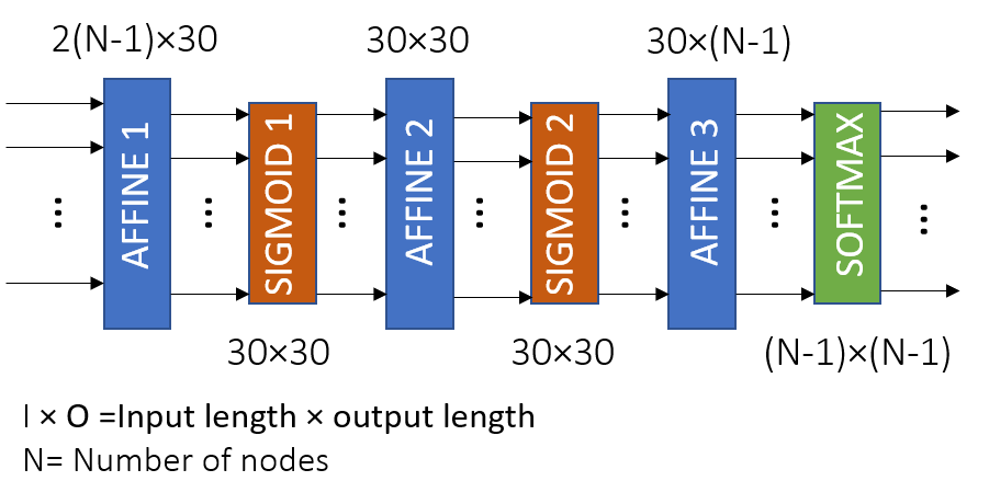
Figure 7: Block diagram of the DNN utilized by the proposed DASA in the experimental study reported in Section V.

V Performance Evaluation

In this section we report an extensive simulation study to evaluate the performance of the proposed algorithm, schematically described in Figs. 6 and 7. To facilitate a fair comparison between the DASA and the classic algorithm (4), the parameters (i.e., $P_{t},q_{i,j},P_{i,j},\left\{\phi_{i}(0)\right\}_{i=1}^{N}$) are identical for the tests of both the analytic algorithm (4) and DASA. We recall that it was shown in Section III that the analytic algorithm fails to achieve full synchronization for the considered scenario. DASA consists of three steps: 1) Data acquisition step; 2) Training step; and 3) Free-run or testing step. At the free-run step, the nodes use their trained DNNs to update their clocks via the update rule (10) with their measured $P_{i,j}(k)$’s and $t_{i,j}(k)$’s.

At startup, corresponding to clock index $k=0$, each node $i$, $i\in\mathcal{I}_{N}$, obtains its initial clock time $\phi_{i}(0)$, generated randomly and uniformly over $[0,T_{i}]$ (see Section III), and the DNN parameters ${\boldsymbol{\theta}}_{i}$ are initialized randomly and uniformly according to the PyTorch default setting. Subsequently, the data acquisition step is applied at all nodes simultaneously. In this step, the nodes compute their clock times for pulse transmissions according to the update rule (10), where the outputs of the local DNNs at the nodes are computed with the corresponding randomly initialized parameters, ${\boldsymbol{\theta}}_{i}$, $i\in\mathcal{I}_{N}$, which are not updated during the this step. We set the duration of the data acquisition interval to $N_{T}=10$ reception cycles. At the end of the data acquisition interval, each node $i$ has a training data set $\mathcal{D}_{i}$. Next, the training step in applied at each node individually, where node $i$ uses the data set $\mathcal{D}_{i}$ to train its individual DNN, $\psi_{{\boldsymbol{\theta_{i}}}}$, according to Algorithm 1.It is emphasized that the data acquisition and the training processes are carried out simultaneously at the individual nodes, as each node applies processing based only on its received pulse timings and powers. We apply training over $E$ epochs, determined such that the individual loss per node $\mathcal{L}_{\mathcal{D}_{i}}({\boldsymbol{\theta}}_{i})$, defined in Eqn. (9), reaches the asymptotic value. After learning the parameters for each DNN, ${\boldsymbol{\theta}}_{i}$, is completed, each node $i$ then continues to update its clock using the rule (10) with weights $\alpha_{i,j}$ computed by applying the trained DNN to its input data. At time $k$, the $N-1$ DNN outputs at node $i$ are computed by $\psi_{{\boldsymbol{\theta}}_{i}}\Big{(}\Big{\{}\big{(}t_{i,j}(k)-\phi_{i}(k),P_{i,j}(k)\big{)}\Big{\}}_{j=1,j\neq i}^{N}\Big{)}$. In the evaluations, we apply the testing step for $2800$ time indexes.

From the numerical evaluations we identified that setting $E=400$ epochs is sufficient for securing convergence. Recalling that each epoch corresponds to a single iteration, it is concluded that convergence is relatively fast. We first consider the behaviour of the clock period after training, for the same network topology with $N=16$ nodes, considered in Section III (see Fig. 3), depicted in Fig. 8 for all $16$ nodes. From the time evolution in Fig. 8(a) it is indeed observed that the nodes’ period convergence is very quick. In Fig. 8(b) we focus in the last $2600$ clock indexes of the testing step: Observe that after convergence, there are still small jumps in the period, which are much smaller than the mean value of the converged period, i.e., $6$ orders of magnitude smaller, hence are considered negligible. It is also interesting to see that once one node experiences a jump in the period, then all other nodes follow. We obtain that at the end of the testing step, the network attains a mean synchronized period of $T_{c,DNN}(2799)=0.00500774$ (computed at the last testing index). Fig. 9(a) depicts the modulus of the clock phases w.r.t $T_{\mbox{\scriptsize nom}}$ across all the nodes, and Fig. 9(b) depicts the modulus of the clock phases w.r.t $T_{c,DNN}$ across all the nodes. It is evident from the figure that the DNN-aided network attains full synchronization w.r.t. $T_{c,DNN}$, which is different from $T_{\mbox{\scriptsize nom}}$. Comparing Fig. 4(b) with Fig. 9(b) we conclude that the proposed DASA offers significantly better performance than the classical approach. Moreover, the performance achieved using the trained DNN is robust to clock period differences and propagation delays.

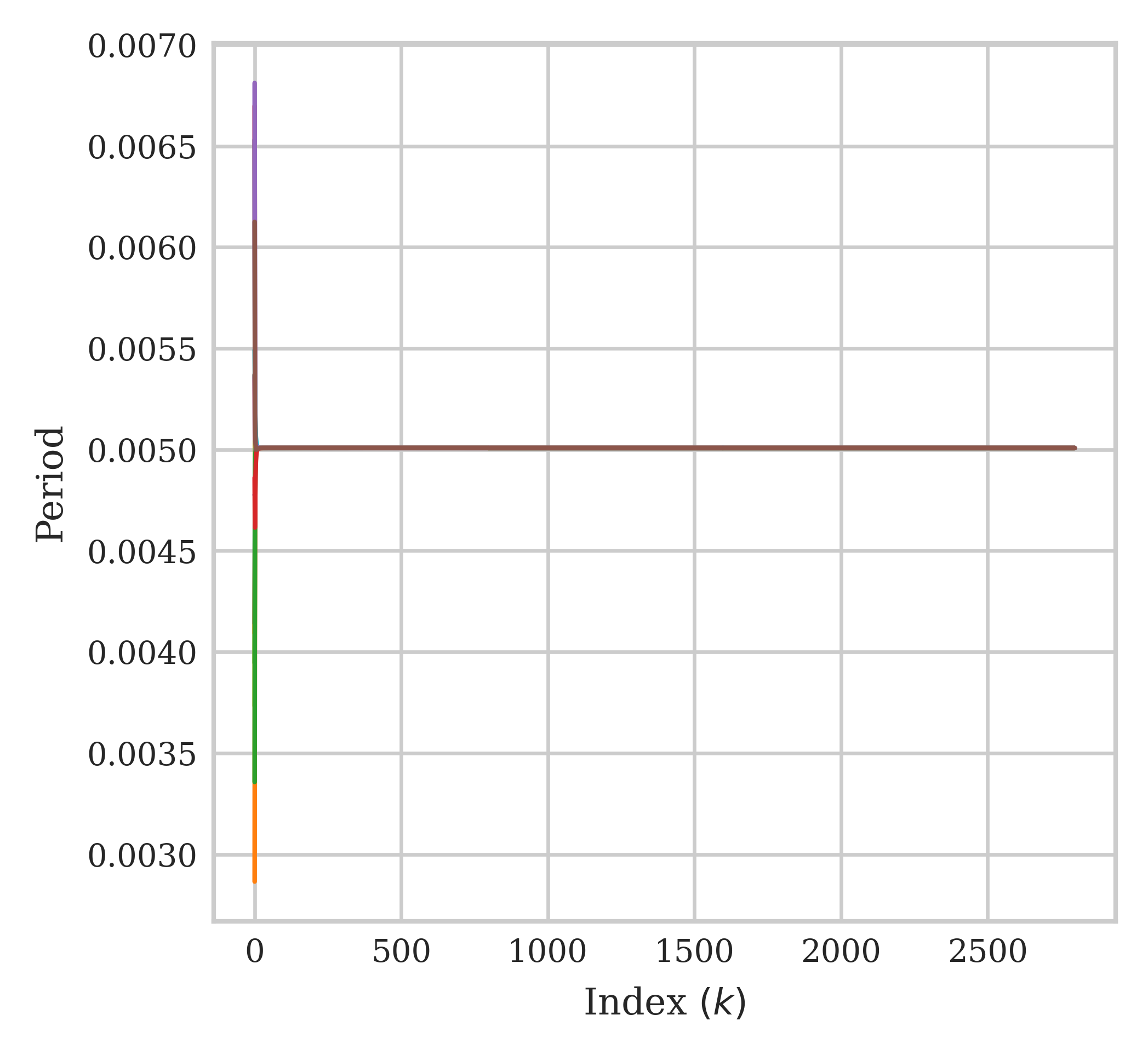
(a)

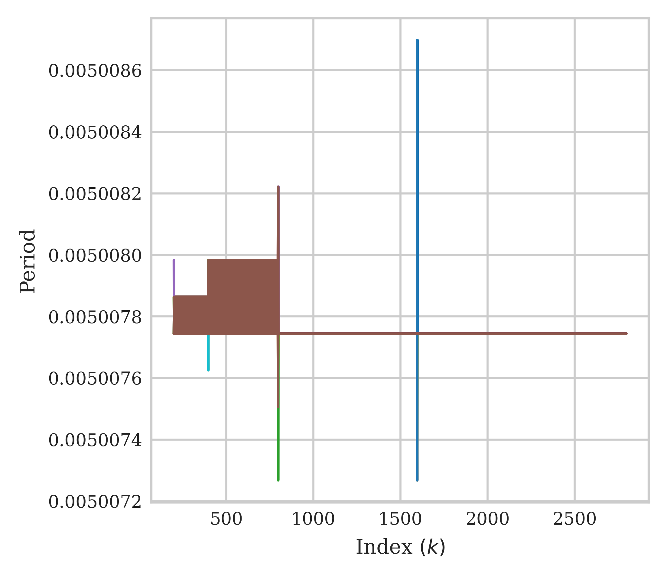
(b)

Figure 8: The evolution of the clock periods for all $16$ nodes using the proposed DASA: (a) The entire test period (time indices 0-2799); and (b) Zoom on the last 2600 time indices (time indices 200-2799).

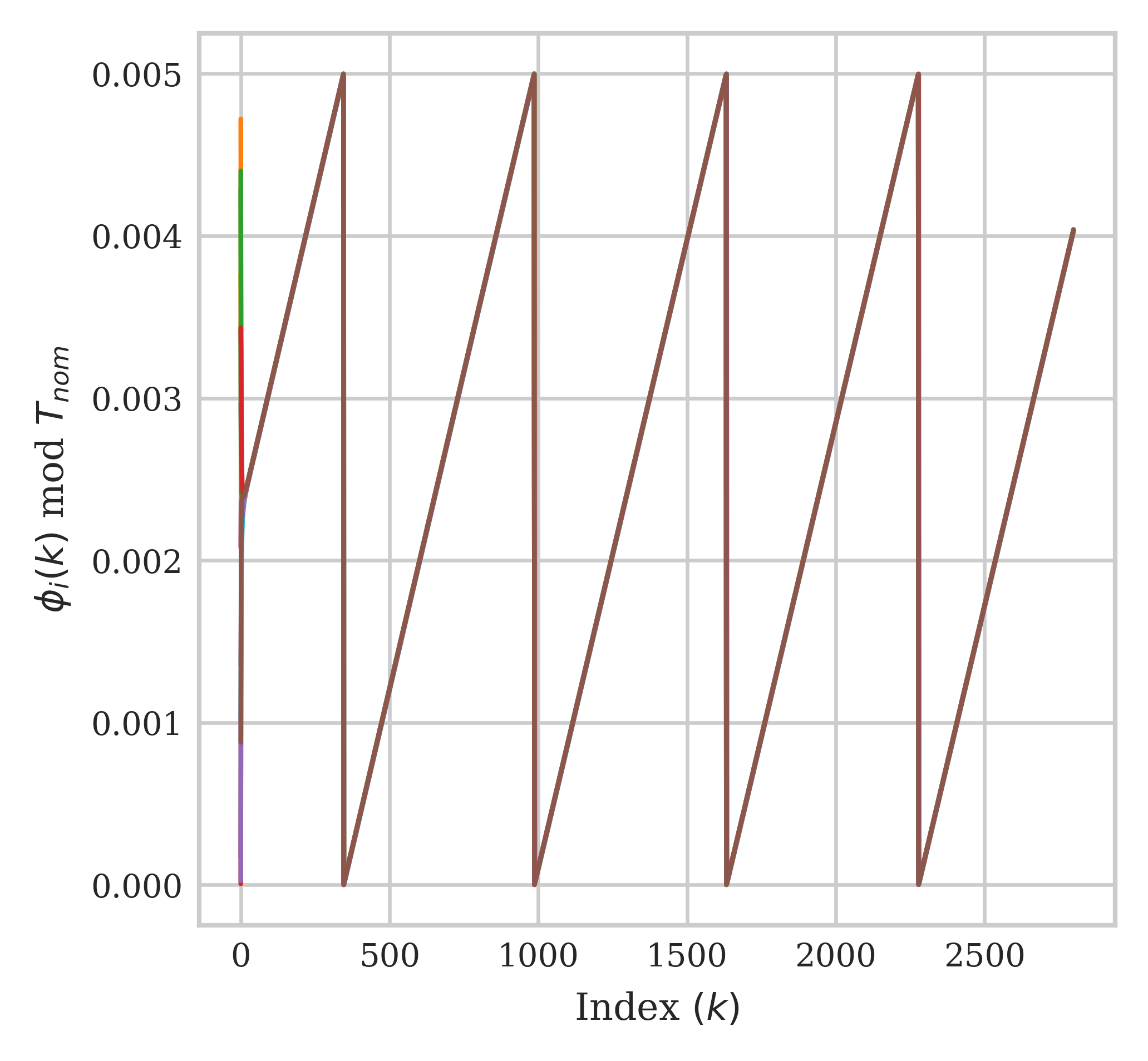
(a)

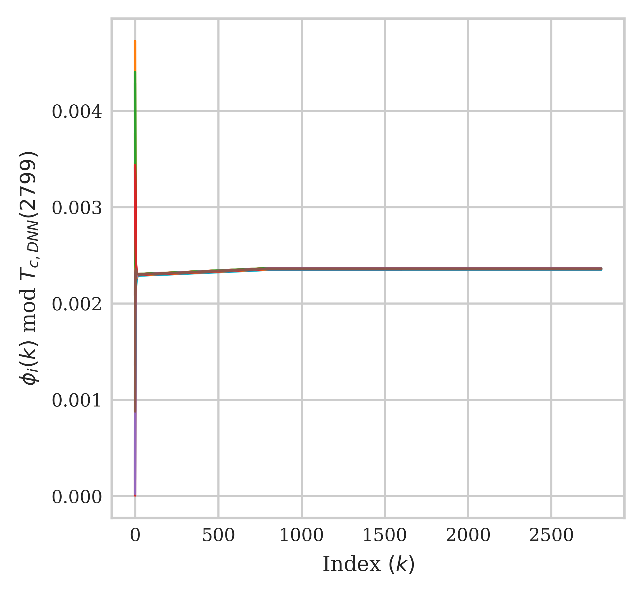
(b)

Figure 9: Modulus of clock phases $\phi_{i}(k)$ for all $N=16$ clocks versus index $k$ using the proposed DASA, (a) w.r.t $T_{\mbox{\scriptsize nom}}$ and (b) w.r.t $T_{c,DNN}(2799)$.

We further compare the performance of both schemes by observing the normalized phase difference (NPD), defined as the difference between the clock phases at the nodes and the clock phase at node $1$, normalized to the mean period, denoted $T_{c}(k)$. Thus, the NPD for node $i$ at time $k$ is defined as:

$$\mbox{NPD}_{i}(k) = {\big{(}\phi_{i}(k)-\phi_{1}(k)\big{)}}/{T_{c}(k)},$$ (11)

$$\mbox{NPD range}(k) \triangleq \mathop{\max}\limits_{i\in\mathcal{I}_{N}}\acs{npd}_{i}(k)-\mathop{\min}\limits_{i\in\mathcal{I}_{N}}\acs{npd}_{i}(k).$$ (12)

where $T_{c}(k)$ depends on the tested algorithm: For the classic algorithm, the NPD is computed w.r.t. its converged period, denoted $T_{c}(k)\equiv T_{c,ANA}(k)$, and for the DASA the NPD is computed w.r.t $T_{c}(k)\equiv T_{c,DNN}(k)$. The NPD values for both schemes at $k=2799$ is depicted in Fig. 10, and the mean and standard deviation (STD) of $\mbox{NPD}_{i}(k)$ over all $i\in\mathcal{I}_{N}$ at $k=2799$ are summarized in Table I. From Fig. 10(a) it is observed that the NPD of analytic algorithm spans a range of $7\%$ of the clock period, with a mean NPD value of $3\%$, while the DASA, depicted in Fig. 10(b), achieves an NPD range of $0.35\%$ and a mean NPD of $0.025\%$. It thus follows that the DASA achieves an improvement by factor of 28 in the standard deviation of the NPD and by a factor of $150$ in the mean NPD. We observe from the table that both schemes achieve frequency synchronization, yet only the DNN-aided network achieves full and accurate synchronization. In the subsequent simulations we test the robustness of the DNN-based scheme to initial clock phase and clock frequency values, and to node mobility, as well as characterize the performance attained when training is done offline.

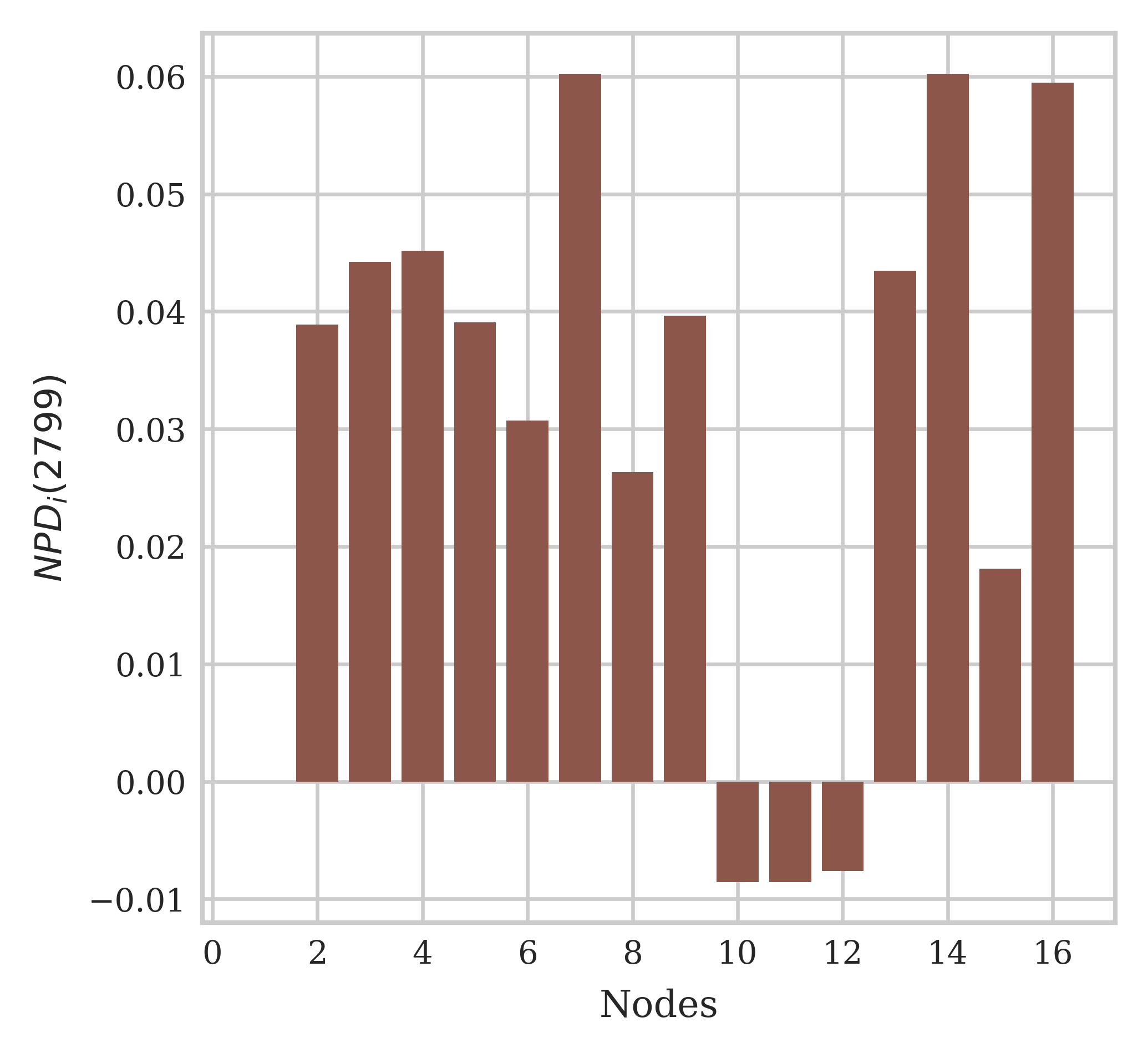
(a)

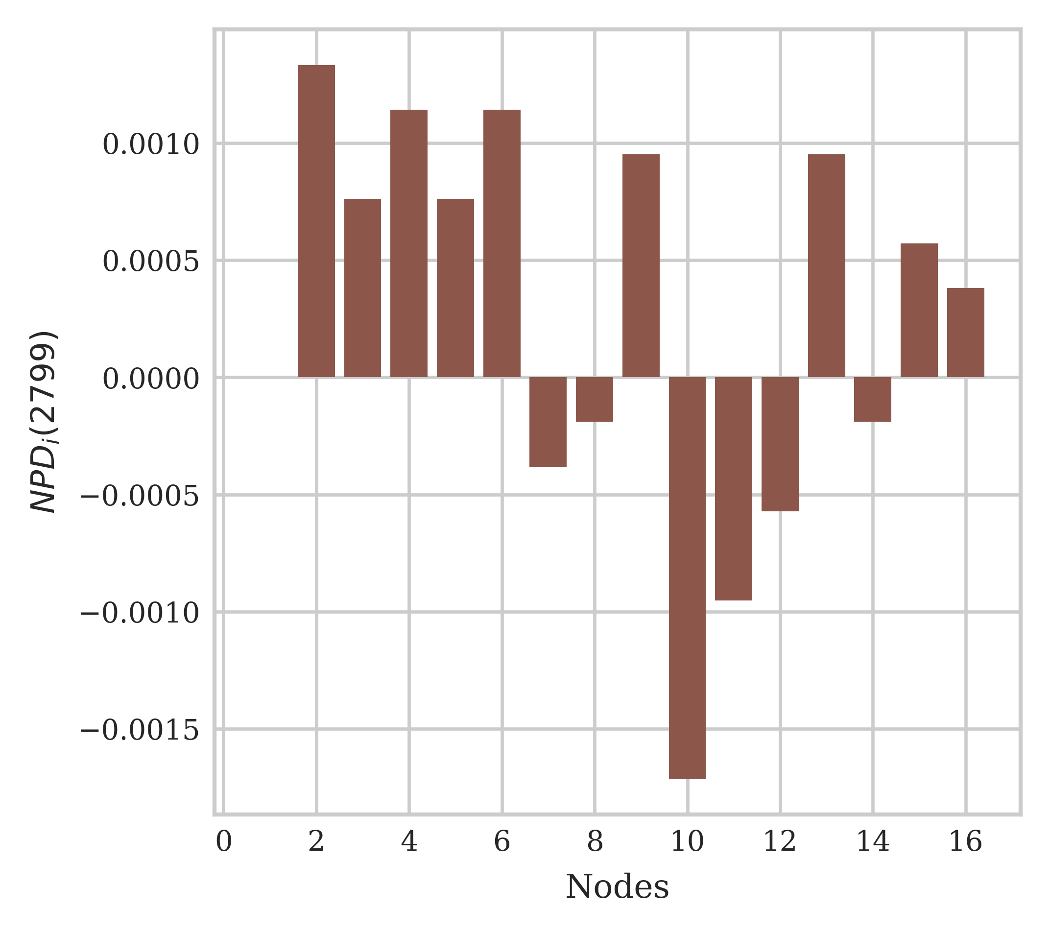
(b)

Figure 10: Normalized phase difference profile for (a) The classical algorithm and (b) DASA.

TABLE I: Performance summary for the classic algorithm and the proposed DASA, at $k=2799$.

	Classical Algorithm	DASA
Mean period	$0.00500208$	$0.00500774$
STD of the period	$5.4715e^{-7}$	$<10^{-10}$
Mean NPD	$3.0052e^{-2}$	$2.4995e^{-4}$
STD of NPD	$2.3738e^{-2}$	$8.3749e^{-4}$

V-A Robustness to Clock Phase and Frequency Resets

In the section we test the robustness of DASA to clock frequency and phase resets during the free-run operation. In the experiments, we first let the nodes learn their DNN networks’ parameters, ${\boldsymbol{\theta}}_{i}$, $i\in\mathcal{I}_{N}$, in an unsupervised manner, as described in Section IV-B. Then, DNNs’ parameters at the nodes remain fixed, while clock resets are applied. Performance in terms of both speed of convergence after a clock reset and the ability to restore full network clock synchronization after a reset are presented for both DASA and the classic algorithm.

In the experiment, both the frequencies and the phases of $30\%$ of the nodes were randomly reset, according to the random distributions detailed in Section III, periodically every $280$ time instants. The resulting clock periods and clock phases for all the nodes in the network are depicted in Figs. 11 and 12, respectively, for the classic algorithm as well as for DASA. It is observed from Fig. 11 that both the classic algorithm and DASA are able to restore frequency synchronization, yet the proposed DASA is able to instantly restore frequency synchronization. We observe from Fig. 12 that the slow frequency synchronization of the classic algorithm induces slow phase synchronization, which is not completed before the next reset occurs, while the newly proposed DASA instantly restores phase synchronization. Is is observed in Fig. 12 that the converged (i.e. steady state) phases of DASA after clock resets are different, yet we clarify that this has no impact on communications network’s performance as all the nodes converge to the same phase within the converged period. It is observed that our proposed DASA is able to instantly restore both the clock frequency and clock phase synchronization (namely, full synchronization), while the classic algorithm requires longer convergence times, and its phases do not complete the convergence process before the next clock reset is applied.

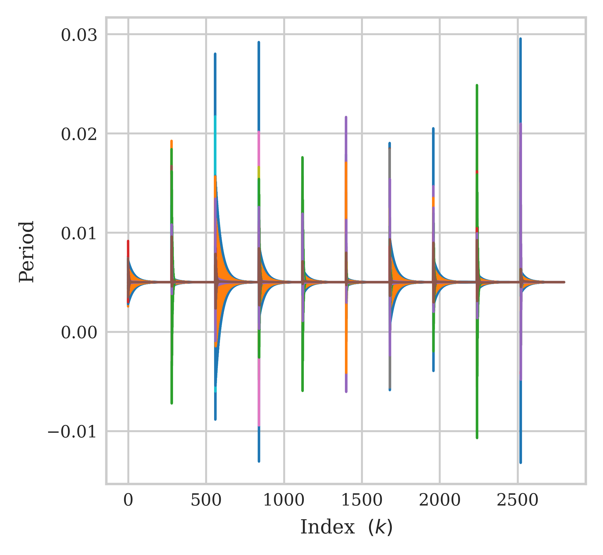
(a)

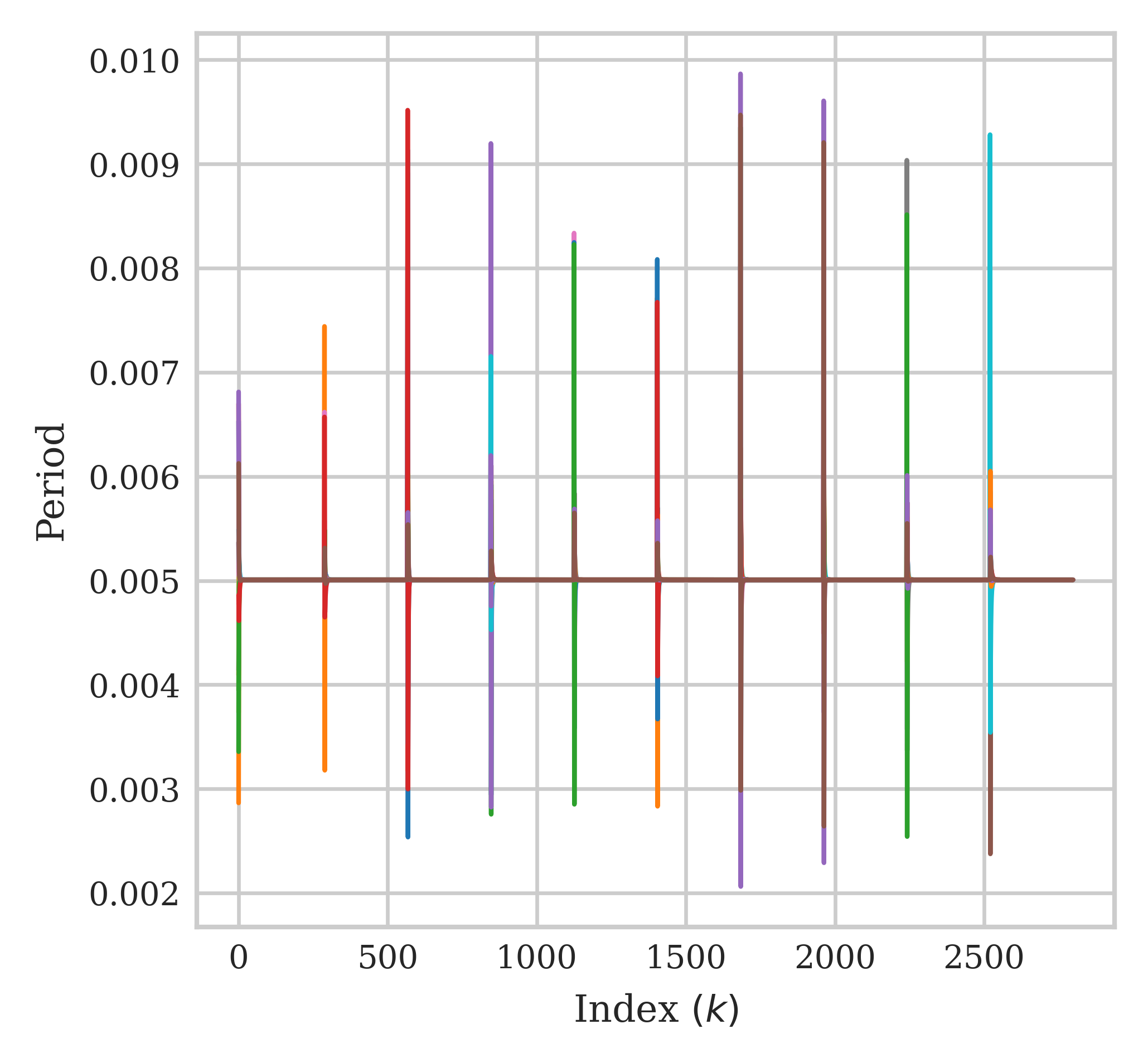
(b)

Figure 11: Convergence of clock frequencies after subsequent clock phase and frequency resets over time index for (a) The classic algorithm; and (b) DASA.

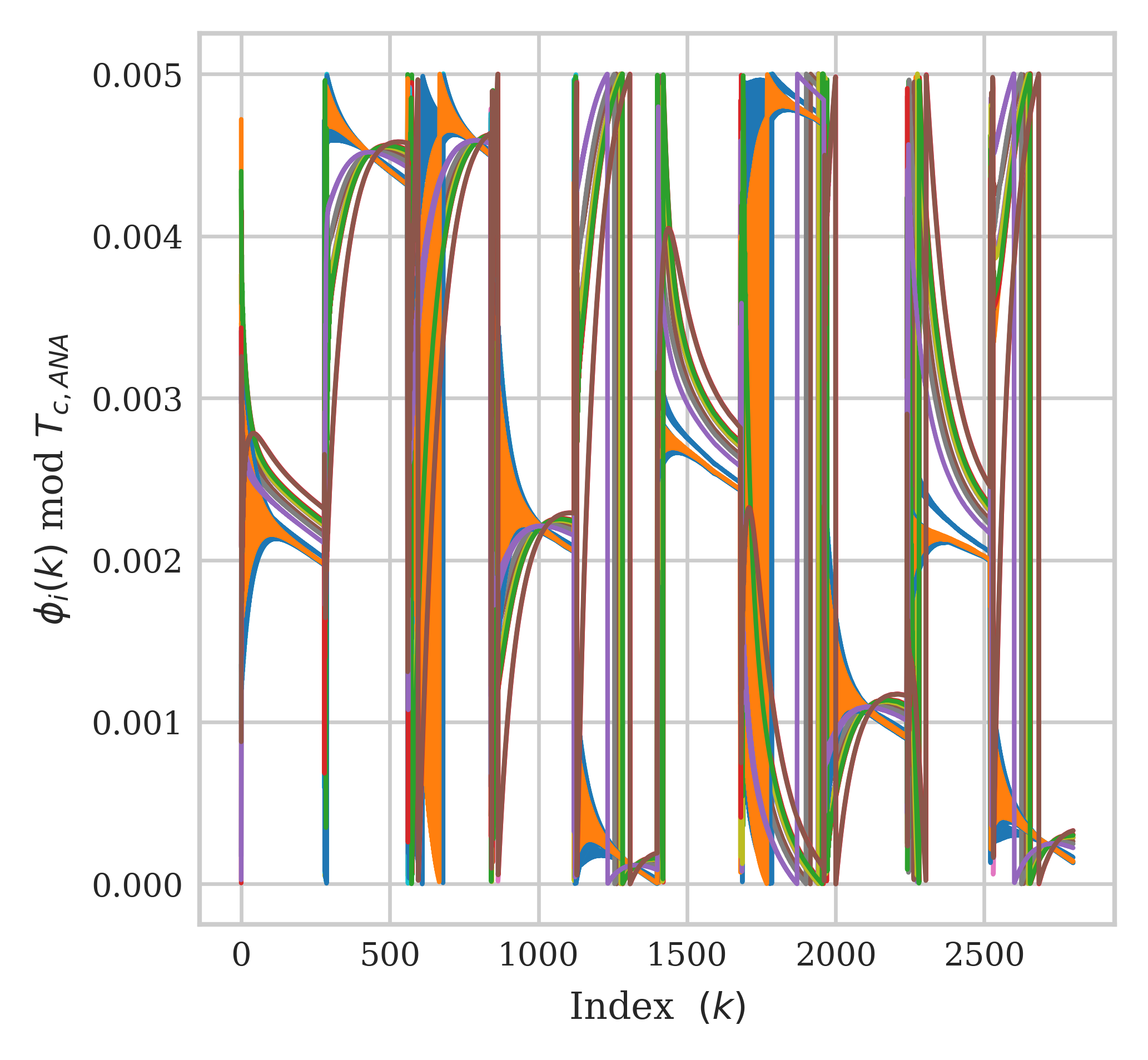
(a)

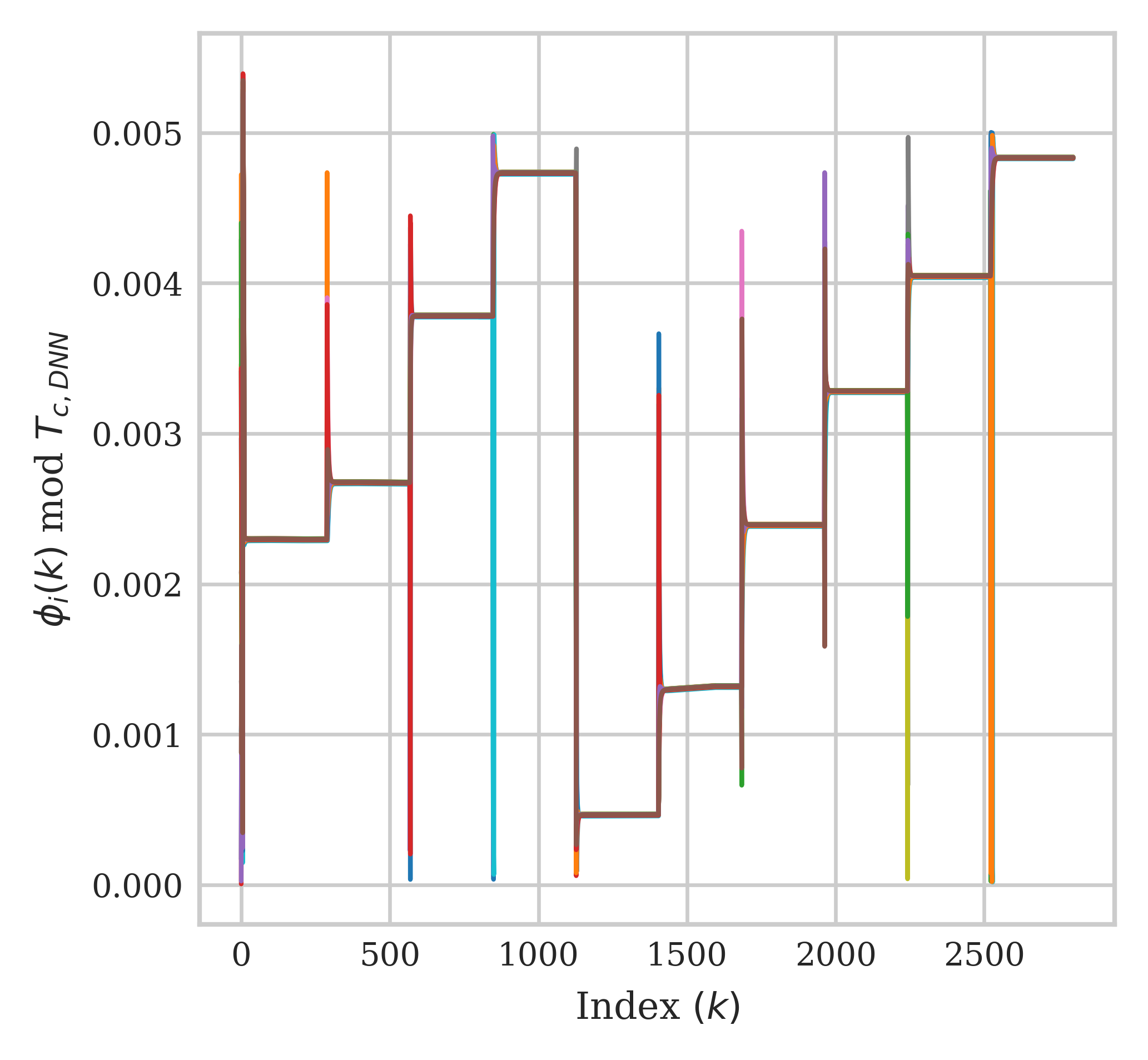
(b)

Figure 12: Modulus of clock phases after subsequent clock phase and period resets over time index for (a) The classic algorithm; and (b) DASA.

Next, we focused on the NPD maintained by DASA during the clock resets. To that aim we plot in Fig. 13 the NPD range, i.e., the difference between the maximal NPD and the minimal NPD, achieved by DASA when both clock phase and period resets are applied. The overall NPD is depicted in Fig. 13(a), where a zoom on the smaller value range, corresponding to the converged state is depicted in Fig. 13(b). Comparing Fig. 13(b) and Fig. 10(b) it is observed that after clock resets DASA achieves the same NPD as in the initial operation after training, namely, clock resets do not degrade the small NPD achieved by DASA.

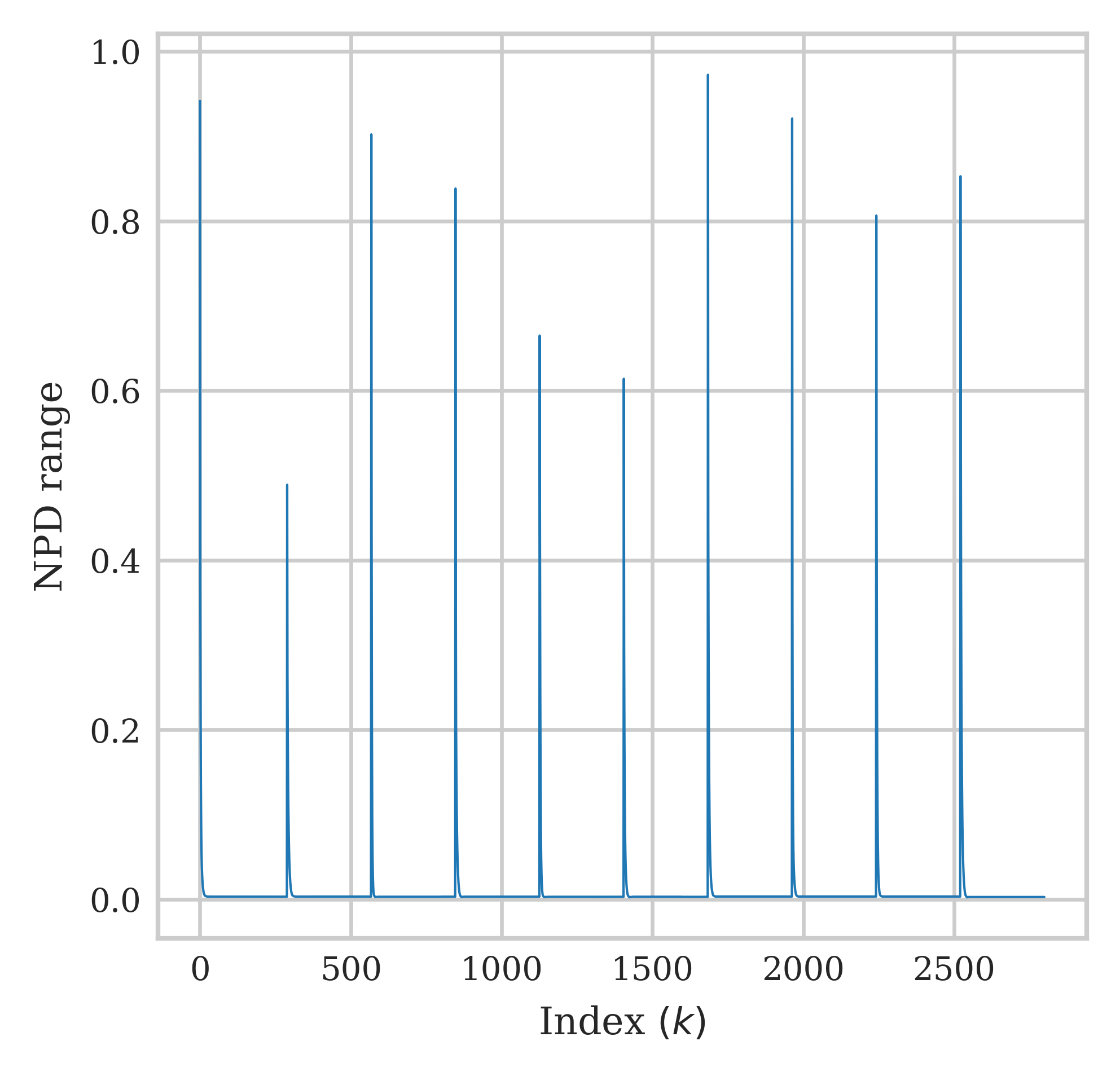
(a)

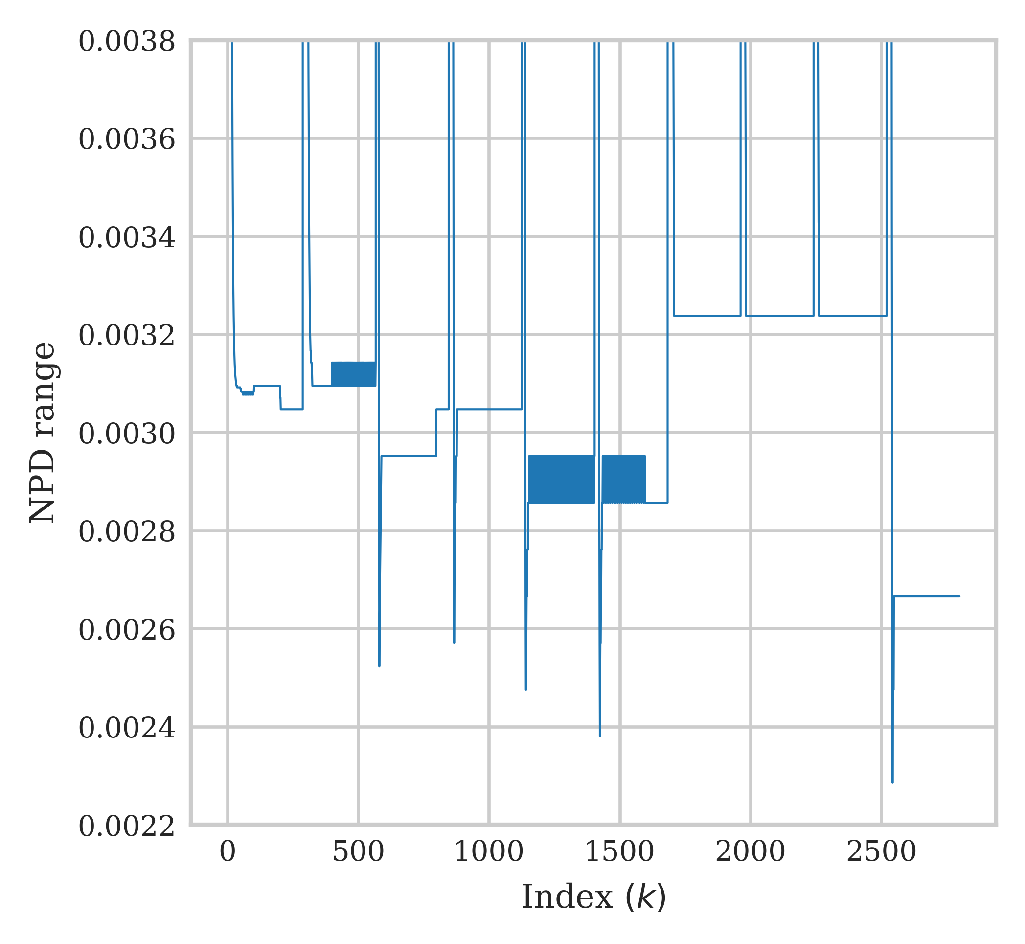
(b)

Figure 13: NPD range over the time index $k$ with subsequent clock phase and period resets over time index and (a) Overall (b) Closeup.

The experiments demonstrate that the proposed DASA is able to facilitate nearly uninterrupted clock phase synchronization, also in presence of random clock resets. These experiments clearly show that DASA is robust to the initial phase and has an outstanding ability to recover from clock phase and frequency variations, which may occur due to e.g., clock temperature changes.

V-B Testing DASA Synchronization Performance with Mobile Nodes

In this subsection we test synchronization performance when some of the nodes are mobile. We let the DNNs at the nodes converge for a stationary scenario (i.e., online training) and then examine synchronization performance when a random subset of $30\%$ of the nodes, selected uniformly, begins moving at a fixed speed, with each mobile given an angular direction. Note that as the nodes move, the received signal powers from and at the moving nodes vary and the received signals at some of the nodes for certain links may fall below the receive threshold, which for the current setup is set to $-114$ dBm. This situation is implemented for such links by setting both the phase difference and the received power to zero. Naturally, this assignment should have a negative impact on synchronization accuracy. In the first experiment, in order to demonstrate the situation of node clustering, the moving nodes were all given the same direction of $95^{\circ}$ and the moving speed was se such that at the end of the simulation each node has traversed $20$ [Km]. Fig. 14 depicts the clock periods and clock phases modulo the instantaneous mean period, $T_{c,DNN}(k)$. It is observed from Fig. 14(a) that frequency synchronization is largely maintained also when nodes are mobile, yet, from Fig. 14(b) we observe a slow drift in the phase modulo $T_{c,DNN}(k)$, which implies that the period slightly varies as the nodes move. It is also noted that despite the phase drift, the nodes are able to maintain close phase values up to a certain time (in this simulation it is time index $1576$, corresponding to a displacement of $10.9$ [Km]), after which the phases split into two separate branches, one consisting of the five mobile i.e., nodes $1$, $2$, $3$, $11$, and $12$, and the second corresponding to the stationary nodes. Checking the connectivity graph for this scenario, it was discovered that at this time index, the network splits into two disconnected sub-networks. Observe that at each sub-network the nodes maintain phase synchronization among themselves.

Lastly, we take a closer look at the NPD performance before network splitting occurs. To that aim, we carried out a new set of $10$ mobility experiments, where the nodes are moving as a speed of $250$ [Km/h], such that at the last time index, $k=2799$, the distance each mobile node traversed was $1$ [Km]. The direction of each moving node is randomly and uniformly selected over $[0,2\pi]$. Fig. 15 depicts the evolution of the NPD range w.r.t $T_{c,DNN}(k)$, for all $10$ experiments. It is observed that the NPD range maintains a very small value, and in fact, in all experiments the NPD range is increased by a factor smaller than $2$ after a $1$ [Km] displacement. Hence, we obtain that DASA exhibits a graceful degradation when the node locations vary, and very good accuracy is maintained also for a large displacement of $1$ [Km]. In fact, it seems that as long as movement does not result in disconnected clusters, DASA generally maintains network synchronization. This demonstrates the robustness of DASA to the topology of the network. This point is of major importance as it implies that moderate node displacements do not require retraining of the network. As a last note in this context, then, based on the mobility experiments and the clock reset experiments we conclude that the optimal weights are dependent on the relative locations of the nodes in the network and only weakly dependent on the clock frequencies and phases.

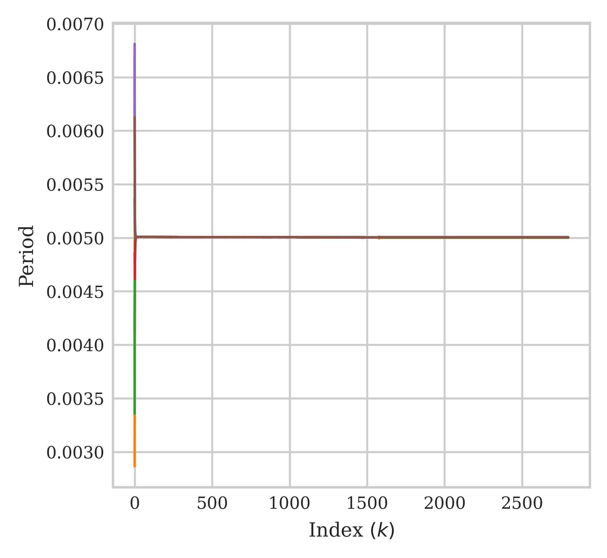
(a)

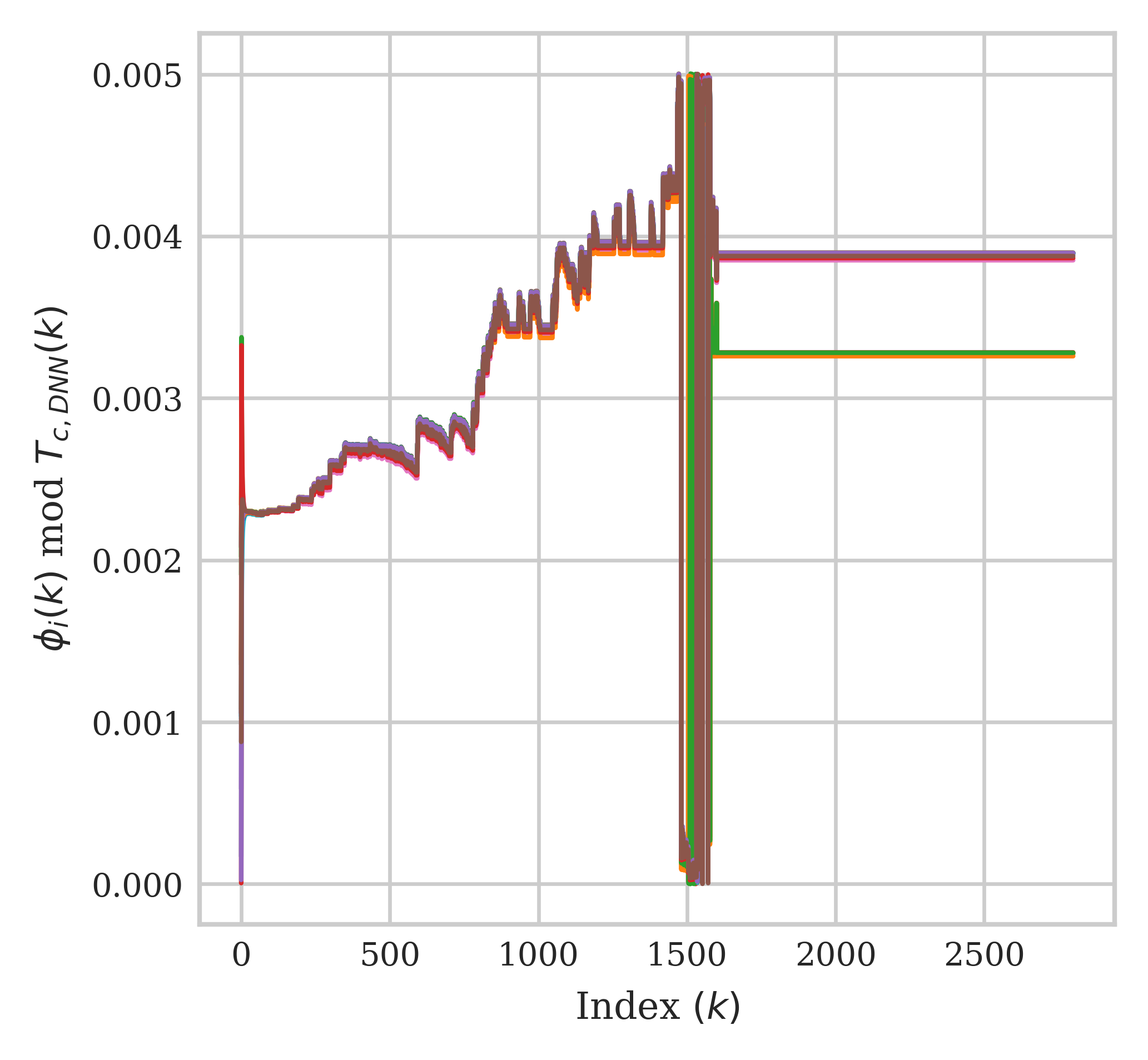
(b)

Figure 14: Clocks’ periods and phases with mobility of $30$% of the nodes at inference w.r.t. the time indices: (a) Clock periods and (b) Clock phases modulo the instantaneous period, $T_{c,DNN}(k)$.

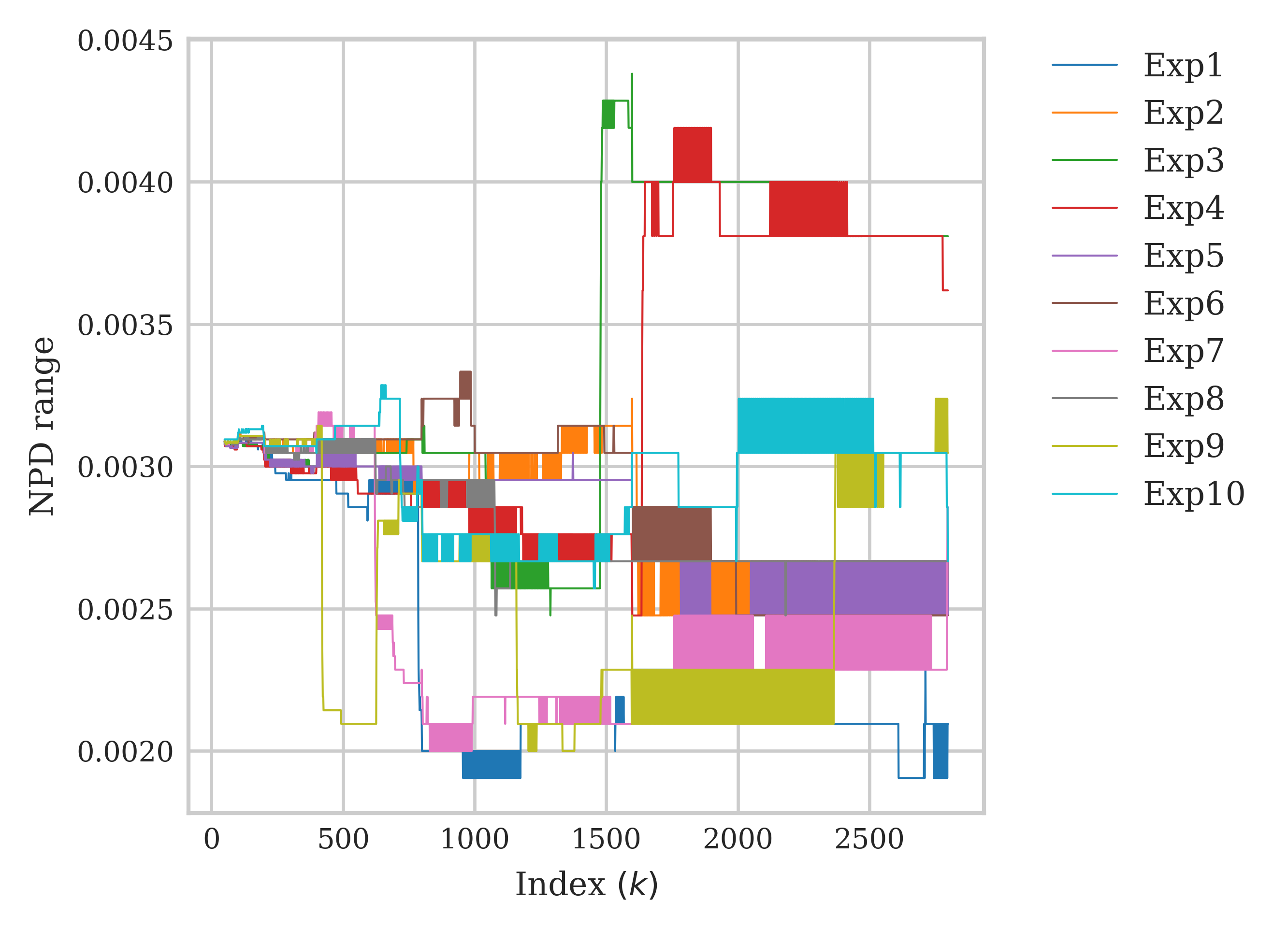
Figure 15: NPD range for $10$ experiments, with online training, where each mobile node moves at a different direction and traverses $1$ [Km] during the simulation.

V-C Offline Training

Next, we examine the possibility of training the DNNs offline over multiple topologies, instead of training online at startup for the actual topology. To implement offline training, we generate a set of $N_{top}$ network topologies, each generated over the same network area of $10$ [km] $\times$ $10$ [km]. For each topology instance, the individual nodes acquire simulated training data consisting of $N_{T}$ time intervals, where at each interval, each node collects $N-1$ inputs. Each input consists of a pair of receive time and received power levels as specified in Eqn. (8). The training data for the $i$’th node over the entire samples of network topologies is denoted as $\mathcal{D}_{i}^{N_{top}}=\left\{\mathcal{D}_{i,n_{top}}\right\}_{n_{top}=1}^{N_{top}}$, where $\mathcal{D}_{i,n_{top}}$ denotes the training data at node $i$ for the $n_{top}$’th topology.

In the previous tests we computed the training loss for a single topology, such that the loss is computed over a single batch and only one step of gradient descent (GD) is applied at each epoch. In contrast, for the offline training we apply the mini-batch stochastic gradient descent (MB-SGD). In this approach, the set $\mathcal{D}_{i}^{N_{top}}$ is divided into mini batches of a fixed size denoted by $N_{samp}$. At each epoch, the MB-SGD at node $i$ operates as follows:

1. A mini-batch is selected for training the node’s DNN in a sequential order.

2. Estimate the average loss over the mini batch topologies, where the loss for the $n_{top}$’th topology, denoted by $\mathcal{L}_{\mathcal{D}_{i,n_{top}}}({\boldsymbol{\theta}}_{i})$ is obtained via Eqn. (9).

3. Compute the gradient and update the DNN’s weights using computed gradient.

4. Repeat steps 1-3 for all mini-batches.

The mini batch training procedure is summarized in Algorithm 2. In the numerical evaluation we used $N_{top}=1000$ topologies, the mini-batch size was set to $N_{samp}=10$; hence, there are $N_{batch}=N_{top}/N_{samples}=100$ mini-batches. For the considered numerical evaluation with MB-SGD, setting $E=3$ epochs was found sufficient to achieve convergence.

Data: Data set $\mathcal{D}_{i}^{N_{top}}$, learning rate $\mu$, initial weights ${\boldsymbol{\theta}}_{i}$, period $T_{i}$, number of epochs $E$

1 for ${\rm epoch}=1$ to $E$ do

2       Randomly shuffle $\mathcal{D}_{i}^{N_{top}}$;

3       for ${\rm batch}=0$ to $N_{batch}-1$ do

4             for $k=1$ to $N_{T}$ do

5                   Forward pass $\left\{\left\{\big{(}t_{i,j}(k),P_{i,j}(k)\big{)}\right\}_{j=1,j\neq i}^{N}\right\}_{n_{top}={\rm batch}\cdot N_{samp}+1}^{({\rm batch}+1)\cdot N_{samp}+1}\in\mathcal{D}_{i}^{N_{top}}$ to obtain $\left\{\psi_{{\boldsymbol{\theta}}_{i,n_{top}}}\right\}_{n_{top}={\rm batch}\cdot N_{samp}+1}^{({\rm batch}+1)\cdot N_{samp}+1}$;

6                   Evaluate $\left\{\phi_{i,n_{top}}(k+1)\right\}_{n_{top}={\rm batch}\cdot N_{samp}+1}^{({\rm batch}+1)\cdot N_{samp}+1}$ applying Eqn. (10) for each $n_{top}$;

7             end for

8            Compute loss $\mathcal{L}_{\mathcal{D}_{i}}({\rm batch},{\boldsymbol{\theta}}_{i})\triangleq\frac{1}{N_{samp}}\mathop{\sum}\limits_{n_{top}={\rm batch}\cdot N_{samp}+1}^{({\rm batch}+1)\cdot N_{samp}+1}\mathcal{L}_{\mathcal{D}_{i,n_{top}}}({\boldsymbol{\theta}}_{i})$ via Eqn. (9);

9             Compute gradient $\nabla_{{\boldsymbol{\theta}}_{i}}\mathcal{L}_{\mathcal{D}_{i}}({\rm batch},{\boldsymbol{\theta}}_{i})$ using back propagation through time;

10             Update weights via ${\boldsymbol{\theta}}_{i}\leftarrow{\boldsymbol{\theta}}_{i}-\mu\cdot\nabla_{{\boldsymbol{\theta}}_{i}}\mathcal{L}_{\mathcal{D}_{i}}({\rm batch},{\boldsymbol{\theta}}_{i})$.

11       end for

12      

13 end for

Algorithm 2 Unsupervised Offline Local Training at Node $i$

After the DNNs have been trained over the set of $N_{top}=1000$ network topologies, DASA was tested for new topologies not included in the training set. Fig. 16 depicts the results for a test topology sample: Fig. 16(a) demonstrates the rapid convergence of the clock periods to a mean synchronized period of $T_{c,DNN}(2799)=0.00500679$. We observe some fluctuations in the periods of the nodes, however, the amplitudes of these variations are three orders of magnitude smaller than the mean synchronized period, hence, these variations are rather negligible. Fig. 16(b) depicts the modulus of the clocks’ phases w.r.t. the mean synchronized period $T_{c,DNN}(2799)$. The figure demonstrates that the proposed DASA with offline training achieves full clock synchronization. Furthermore, its performance is significantly better than the performance of the classical algorithm, as it is robust to propagation delays. Fig. 16(c), depicts a closeup of the NPD range. Observe that DASA achieves an NPD range of $0.41\%$ at the first few time indices and a converged NPD range of $0.4\%$ at later time indices ($k\geq 850$). Lastly, Fig 16(d) depicts a snapshot of the NPD values across nodes at time $k=2799$. From the figure, we again note that the NPD range is $0.4\%$ across the nodes, we also see that the mean value is $0.064\%$. The performance of DASA for this test is summarized in Table II. Comparing with the online training results in Table I we note that period accuracy is similar for both scenarios; the main benefit of online training is a smaller NPD, by a factor of $2.5$, and an NPD STD smaller by a factor of $1.3$.

TABLE II: Performance summary of the proposed DASA, at index k=2799 for a test network topology with offline training setup.

	DASA
Mean period	$0.00500679$
STD of the period	$<10^{-10}$
Mean NPD	$6.4285e^{-4}$
STD of NPD	$1.1124e^{-3}$

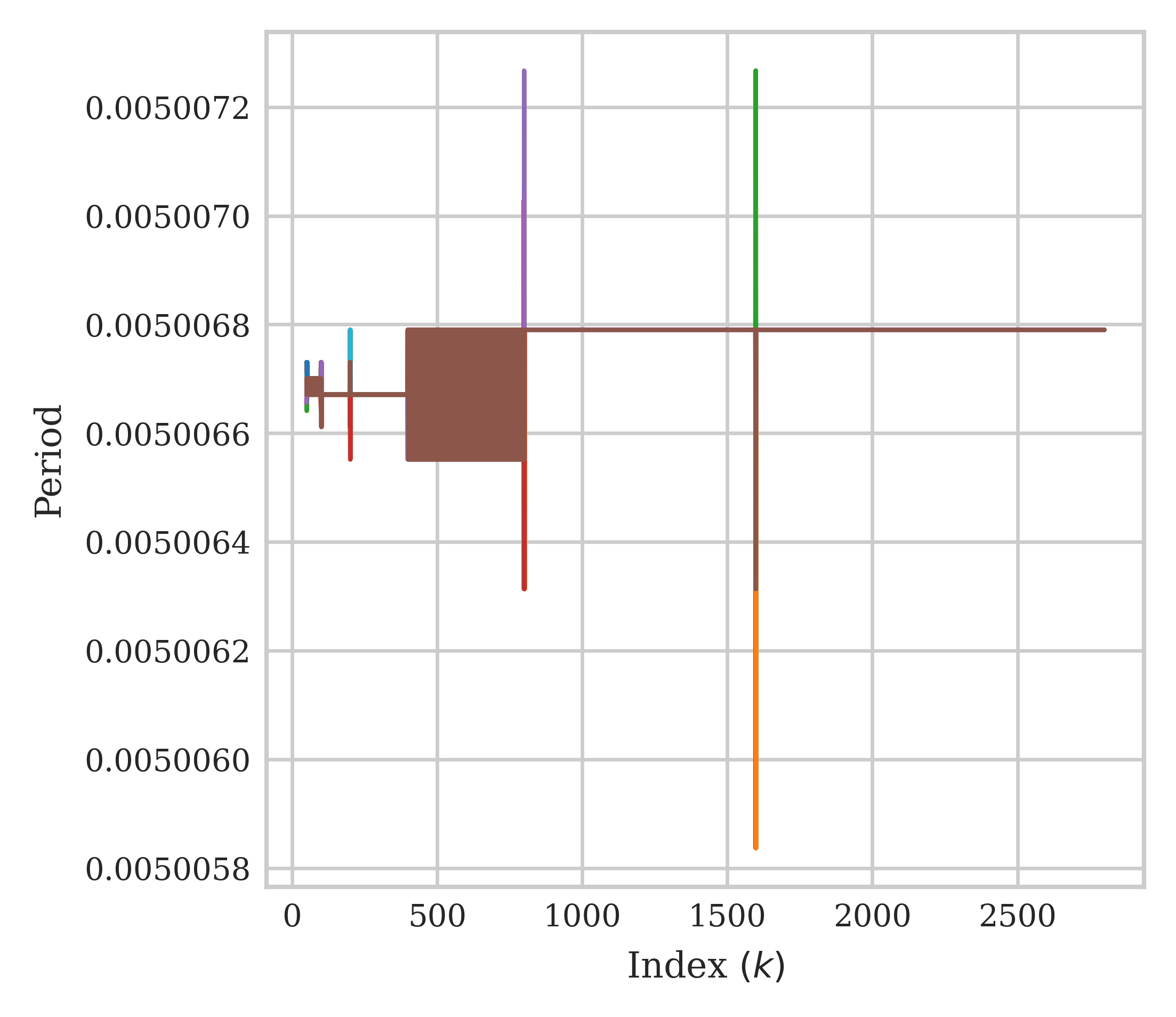
(a)

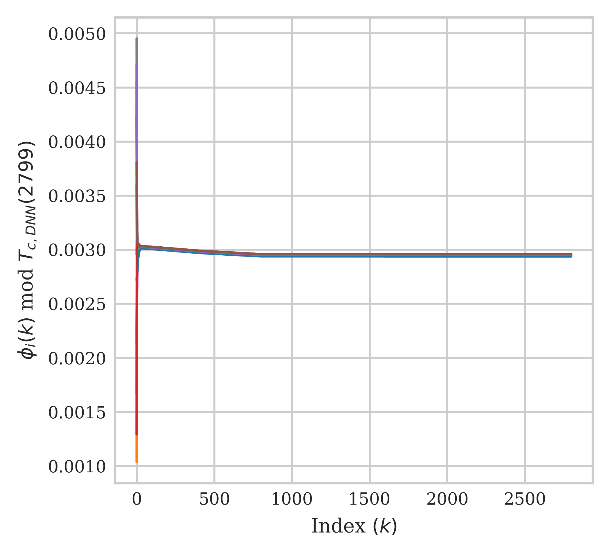
(b)

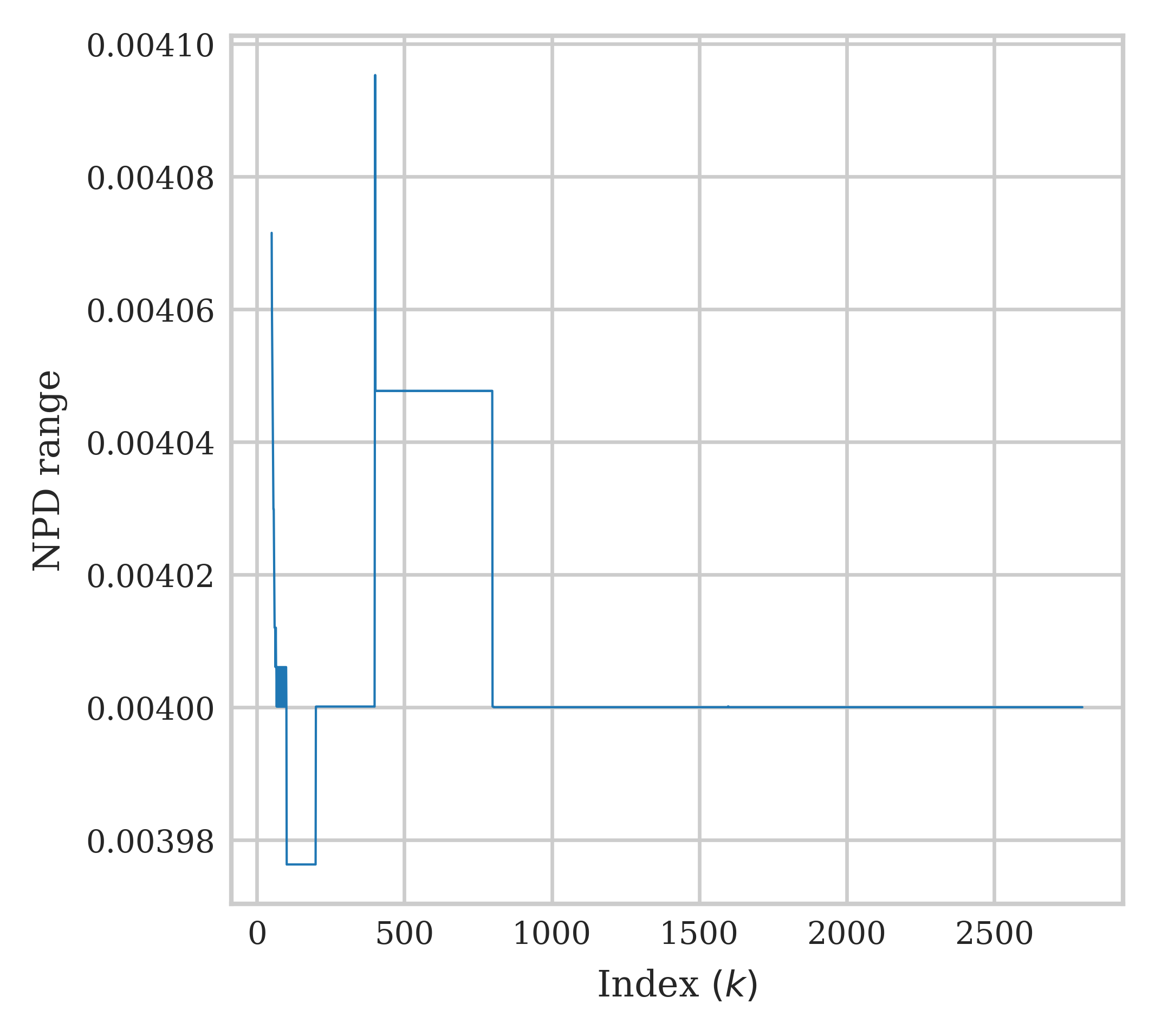
(c)

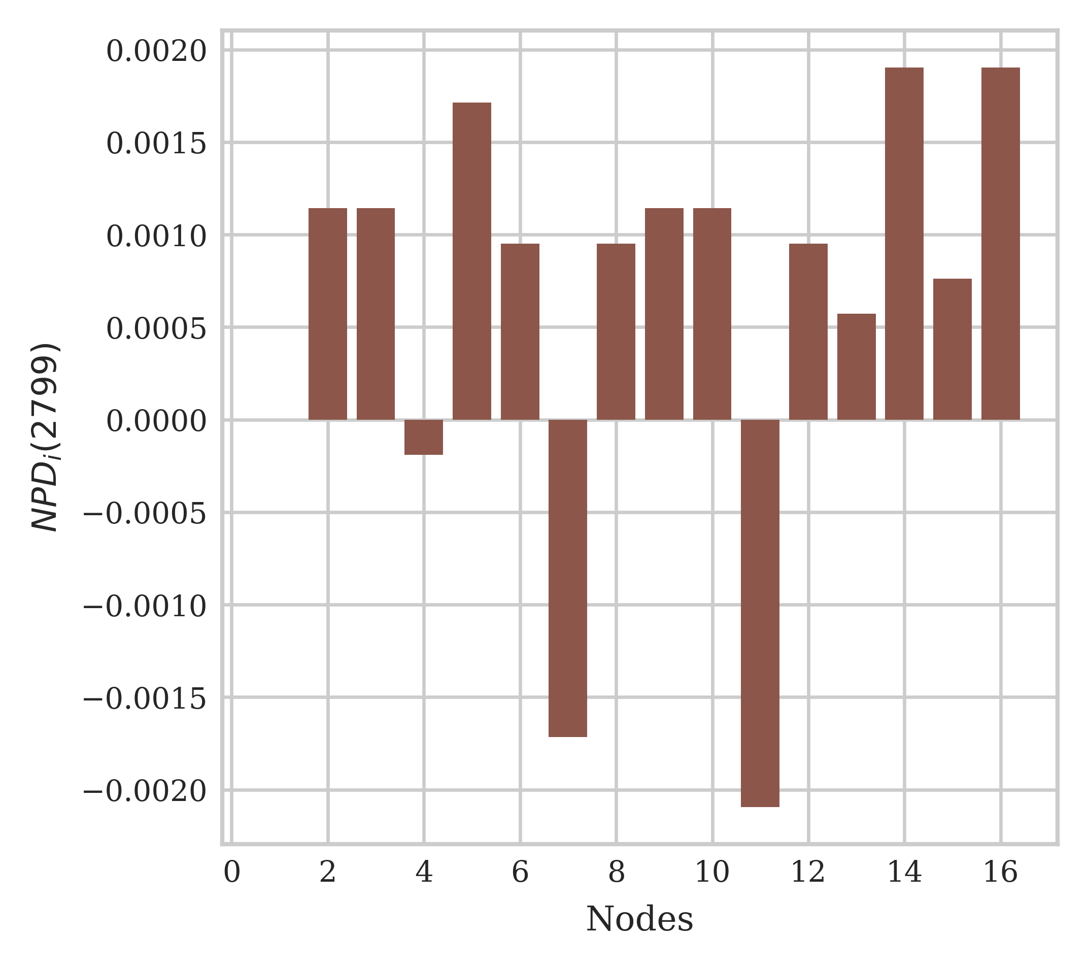
(d)

Figure 16: Performance of the DASA for a test topology after offline training: (a) Clock periods, (b) Clock phases modulo $T_{c,DNN}(2799)$, (c) NPD range, and (d) $\big{\{}NPD_{i}(2799)\big{\}}_{i=1}^{N}6$.

Lastly, we examine synchronization performance for the topology used in Fig. 16, with mobility, as was done in Fig. 15, i.e., we randomly and uniformly select $30\%$ of the nodes, and each selected nodes a random angular direction is selected uniformly over $[0,2\pi)$. The moving nodes travel at a fixed speed, such that at the end of the simulation, each moving node has travelled $1$ [Km]. Fig. 17 depicts the evolution of NPD range with time, as was done in Fig. 15 for online training. Specifically, it was observed that at displacement of $1$ [Km], The NPD range increases by a factor smaller than $2$, similar to online training. Thus, we conclude that offline training also offers excellent robustness to node mobility.

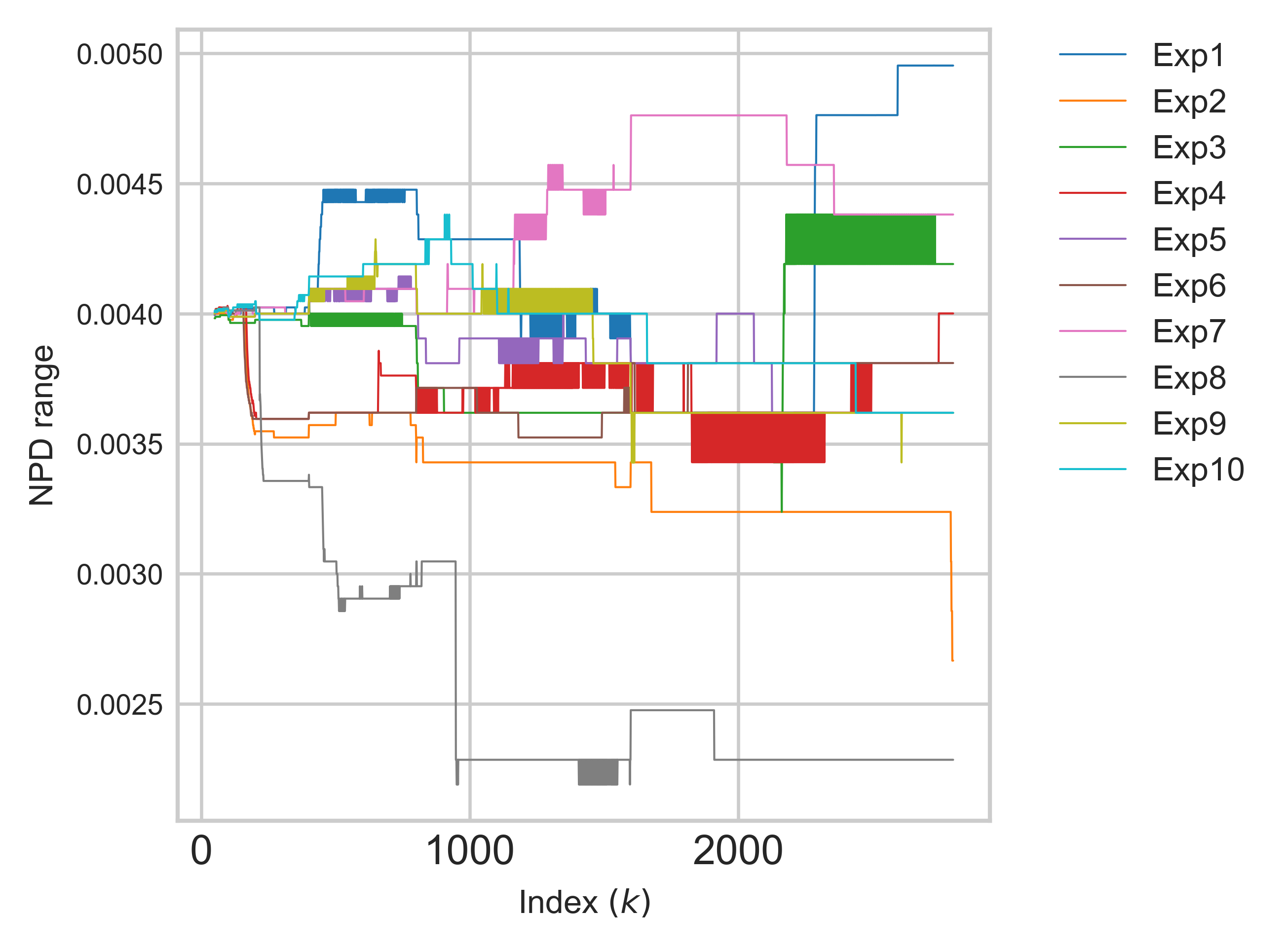
Figure 17: NPD range for $10$ experiments, with each mobile node moving at a different direction and traverses $1$ [Km] during the simulation.

VI Conclusions

This work considers network clock synchronization for wireless networks via pulse coupled PLLs at the nodes. The widely studied classic synchronization scheme based on the update rule (4) is known to fail in achieving full synchronization for networks with non-negligible propagation delays, and/or the clock frequency differences among the nodes, resulting in clusters of nodes synchronized among themselves, while the clocks of nodes belonging to different clusters are not phase-synchronized. In this work, we propose an algorithm, abbreviated as DASA, which replaces the analytically computed $\alpha_{i,j}$ coefficients of the classic algorithm with weights learned using DNNs, such that learning is done is an unsupervised and distributed manner, and requires a very short training period. These properties make the proposed algorithm very attractive for practical implementation. With the proposed DNN-aided synchronization scheme, each node determines its subsequent clock phase using its own clock and the timings of the pulses received from the other nodes in the network. Numerical results show that when there are propagation delays and clock frequency differences between the nodes, both the proposed DASA and the classic analytically-based scheme achieve frequency synchronization, however only the proposed DASA is able to attain full synchronization of both the frequency and phase with a very high accuracy. It was demonstrated that DASA maintains synchronization also in the presence of clock frequency and phase resets occurring at a subset of the nodes. Moreover, DASA was also shown to maintain accurate synchronization when only part of the nodes is mobile. Lastly we evaluated the relevance of offline training to the considered scenario: It was shown that offline training achieves full synchronization, with only a small degradation in the NPD and the NPD range, compared to online training.

References

- [1] J. Perry, A. Ousterhout, H. Balakrishnan, D. Shah, and H. Fugal, “Fastpass: A centralized ”zero-queue” datacenter network,” in Proc. of the ACM SIGCOMM Conference, 2014, pp. 307–318.
- [2] Y. Geng, S. Liu, Z. Yin, A. Naik, B. Prabhakar, M. Rosenblum, and A. Vahdat, “Exploiting a natural network effect for scalable, fine-grained clock synchronization,” in Proc. of the USENIX Symp. on Networked Systems Design and Implementation (NSDI), 2018, pp. 81–94.
- [3] M. Akhlaq and T. R. Sheltami, “RTSP: An accurate and energy-efficient protocol for clock synchronization in WSNs,” IEEE Transactions on Instrumentation and Measurement, vol. 62, no. 3, pp. 578–589, 2013.
- [4] Y.-C. Wu, Q. Chaudhari, and E. Serpedin, “Clock synchronization of wireless sensor networks,” IEEE Signal Processing Magazine, vol. 28, no. 1, pp. 124–138, 2010.
- [5] M. Raza, N. Aslam, H. Le-Minh, S. Hussain, Y. Cao, and N. M. Khan, “A critical analysis of research potential, challenges, and future directives in industrial wireless sensor networks,” IEEE Communications Surveys & Tutorials, vol. 20, no. 1, pp. 39–95, 2017.
- [6] O. Simeone, U. Spagnolini, Y. Bar-Ness, and S. H. Strogatz, “Distributed synchronization in wireless networks,” IEEE Signal Processing Magazine, vol. 25, no. 5, pp. 81–97, 2008.
- [7] F. Sivrikaya and B. Yener, “Time synchronization in sensor networks: a survey,” IEEE network, vol. 18, no. 4, pp. 45–50, 2004.
- [8] A. K. Karthik and R. S. Blum, “Recent advances in clock synchronization for packet-switched networks,” Foundations and Trends in Signal Processing, vol. 13, no. 4, pp. 360–443, 2020.
- [9] M. Maróti, B. Kusy, G. Simon, and A. Lédeczi, “The flooding time synchronization protocol,” in Proceedings of the 2nd international conference on Embedded networked sensor systems, 2004, pp. 39–49.
- [10] “IEEE standard for a precision clock synchronization protocol for networked measurement and control systems,” IEEE Std 1588-2008 (Revision of IEEE Std 1588-2002), pp. 1–269, 2008.
- [11] D. Mills, J. Martin, J. Burbank, and W. Kasch, “Network time protocol version 4: Protocol and algorithms specification,” Network, 2010.
- [12] I. S. Association et al., “IEEE standard for local and metropolitan area networks - timing and synchronization for time-sensitive applications in bridged local area networks,” IEEE Std 802.1AS-2011, pp. 1–292, 2011.
- [13] R. Pigan and M. Metter, Automating with PROFINET: Industrial communication based on Industrial Ethernet. John Wiley & Sons, 2008.
- [14] Y.-W. Hong and A. Scaglione, “A scalable synchronization protocol for large scale sensor networks and its applications,” IEEE Journal on selected areas in communications, vol. 23, no. 5, pp. 1085–1099, 2005.
- [15] E. Koskin, D. Galayko, O. Feely, and E. Blokhina, “Generation of a clocking signal in synchronized all-digital PLL networks,” IEEE Transactions on Circuits and Systems II: Express Briefs, vol. 65, no. 6, pp. 809–813, 2018.
- [16] N. Shlezinger, J. Whang, Y. C. Eldar, and A. G. Dimakis, “Model-based deep learning,” preprint arXiv:2012.08405, 2020.
- [17] N. Shlezinger, N. Farsad, Y. C. Eldar, and A. J. Goldsmith, “Model-based machine learning for communications,” arXiv preprint arXiv:2101.04726, 2021.
- [18] N. Shlezinger, Y. C. Eldar, and S. P. Boyd, “Model-based deep learning: On the intersection of deep learning and optimization,” arXiv preprint arXiv:2205.02640, 2022.
- [19] A. Vaswani, N. Shazeer, N. Parmar, J. Uszkoreit, L. Jones, A. N. Gomez, Ł. Kaiser, and I. Polosukhin, “Attention is all you need,” Advances in neural information processing systems, vol. 30, 2017.
- [20] M. K. Maggs, S. G. O’keefe, and D. V. Thiel, “Consensus clock synchronization for wireless sensor networks,” IEEE sensors Journal, vol. 12, no. 6, pp. 2269–2277, 2012.
- [21] C. Royle, C. Godsil, and G. Royle, Algebraic Graph Theory, ser. Graduate Texts in Mathematics. Springer, 2001.
- [22] L. Moreau, “Stability of multiagent systems with time-dependent communication links,” IEEE Transactions on automatic control, vol. 50, no. 2, pp. 169–182, 2005.
- [23] W. Ren and R. W. Beard, “Consensus seeking in multiagent systems under dynamically changing interaction topologies,” IEEE Transactions on automatic control, vol. 50, no. 5, pp. 655–661, 2005.
- [24] Y. Cao, W. Yu, W. Ren, and G. Chen, “An overview of recent progress in the study of distributed multi-agent coordination,” IEEE Transactions on Industrial informatics, vol. 9, no. 1, pp. 427–438, 2012.
- [25] M. A. Alvarez and U. Spagnolini, “Distributed time and carrier frequency synchronization for dense wireless networks,” IEEE Transactions on Signal and Information Processing over Networks, vol. 4, no. 4, pp. 683–696, 2018.
- [26] F. Tong and Y. Akaiwa, “Theoretical analysis of inter-basestation-synchronization system,” in Proceedings of ICUPC’95-4th IEEE International Conference on Universal Personal Communications, 1995, pp. 878–882.
- [27] E. Sourour and M. Nakagawa, “Mutual decentralized synchronization for intervehicle communications,” IEEE Transactions on Vehicular Technology, vol. 48, no. 6, pp. 2015–2027, 1999.
- [28] R. Olfati-Saber and R. M. Murray, “Consensus problems in networks of agents with switching topology and time-delays,” IEEE Transactions on automatic control, vol. 49, no. 9, pp. 1520–1533, 2004.
- [29] D. Tetreault-La Roche, B. Champagne, I. Psaromiligkos, and B. Pelletier, “On the use of distributed synchronization in 5G device-to-device networks,” in 2017 IEEE International Conference on Communications (ICC), 2017, pp. 1–7.
- [30] K. D. Pham, “Stochastic power controls for distributed pulse-coupled synchronization,” in 2017 IEEE Aerospace Conference, 2017, pp. 1–9.
- [31] O. Simeone and U. Spagnolini, “Distributed time synchronization in wireless sensor networks with coupled discrete-time oscillators,” EURASIP Journal on Wireless Communications and Networking, vol. 2007, pp. 1–13, 2007.
- [32] I. E. L. Hulede and H. M. Kwon, “Distributed network time synchronization: Social learning versus consensus,” IEEE Transactions on Signal and Information Processing over Networks, vol. 7, pp. 660–675, 2021.
- [33] S. B. Amor, S. Affes, F. Bellili, U. Vilaipornsawai, L. Zhang, and P. Zhu, “Joint ML time and frequency synchronization for distributed mimo-relay beamforming,” in IEEE Wirel. Commu. and Net. Conf. (WCNC), 2019, pp. 1–8.
- [34] W. Jakes, Microwave Mobile Communications, ser. IEEE Press classic reissue. Wiley, 1974.
- [35] P. Palà-Schönwälder, J. Bonet-Dalmau, A. López-Riera, F. X. Moncunill-Geniz, F. del Águila-López, and R. Giralt-Mas, “Superregenerative reception of narrowband fsk modulations,” IEEE Trans. Circuits Syst. I Regul. Pap., vol. 62, no. 3, pp. 791–798, 2015.
- [36] N. Naik, “Lpwan technologies for iot systems: choice between ultra narrow band and spread spectrum,” in IEEE International Systems Engineering Symposium (ISSE), 2018, pp. 1–8.
- [37] A. C. Scogna, H. Shim, J. Yu, C. Oh, S. Cheon, N. Oh, and D. Kim, “Rfi and receiver sensitivity analysis in mobile electronic devices,” in DesignCon, vol. 7, 2017, pp. 1–6.
- [38] N. Samuel, T. Diskin, and A. Wiesel, “Learning to detect,” IEEE Transactions on Signal Processing, vol. 67, no. 10, pp. 2554–2564, 2019.
- [39] I. Sutskever, Training recurrent neural networks. University of Toronto Toronto, ON, Canada, 2013.
- [40] L. Deng, G. Li, S. Han, L. Shi, and Y. Xie, “Model compression and hardware acceleration for neural networks: A comprehensive survey,” Proc. IEEE, vol. 108, no. 4, pp. 485–532, 2020.
- [41] T. Raviv, S. Park, N. Shlezinger, O. Simeone, Y. C. Eldar, and J. Kang, “Meta-ViterbiNet: Online meta-learned Viterbi equalization for non-stationary channels,” in Proc. IEEE ICC, 2021.
- [42] T. Raviv, S. Park, O. Simeone, Y. C. Eldar, and N. Shlezinger, “Online meta-learning for hybrid model-based deep receivers,” arXiv preprint arXiv:2203.14359, 2022.