Evolution of Activation Functions for Deep Learning-Based Image Classification

Abstract.

Activation functions (AFs) play a pivotal role in the performance of neural networks. The Rectified Linear Unit (ReLU) is currently the most commonly used AF. Several replacements to ReLU have been suggested but improvements have proven inconsistent. Some AFs exhibit better performance for specific tasks, but it is hard to know a priori how to select the appropriate one(s). Studying both standard fully connected neural networks (FCNs) and convolutional neural networks (CNNs), we propose a novel, three-population, coevolutionary algorithm to evolve AFs, and compare it to four other methods, both evolutionary and non-evolutionary. Tested on four datasets—MNIST, FashionMNIST, KMNIST, and USPS—coevolution proves to be a performant algorithm for finding good AFs and AF architectures.

1. Introduction

Artifical Neural Networks (ANNs), and, specifically, Deep Neural Networks (DNNs), have gained much traction in recent years and are now being effectively put to use in a variety of applications. Considerable work has been done to improve training and testing performance, including various initialization techniques, weight-tuning algorithms, different architectures, and more. However, one hyperparameter is usually left untouched: the activation function (AF). While recent work has seen the design of novel AFs (Agostinelli et al., 2014; Saha et al., 2019; Sharma and Sharma, 2017; Sipper, 2021), the Rectified Linear Unit (ReLU) remains by far the most commonly used one, mainly due to its overcoming the vanishing-gradient problem, thus affording faster learning and better performance.

AFs are crucial first and foremost because they transform a neural network from a simple linear algorithm into a non-linear one, thus allowing the network to learn complex mappings and functions. If the AFs of a neural network were removed, the whole architecture could be reduced to a linear operation on its input, with very limited use. Traditionally, the most commonly used AFs were sigmoid functions—such as logistic and hyperbolic tangent—which are bounded, differentiable, and monotonic. Such functions are prone to the vanishing-gradient problem (Hochreiter, 1998): when the function value is either too high or too low, the derivative becomes very small, and learning becomes very poor. To address this issue, different functions have been developed, the most prominent of which being the ReLU. Though it has proven highly performant, the ReLU is susceptible to a problem known as “dying” (Lu et al., 2019): because all negative values are mapped to zero, there might be a scenario where a large number of ReLU neurons only output a 0 value. It might cause the entire network to “die”, resulting in a constant function.

Different variants of ReLU, such as PReLU (Zhang et al., 2018) and Leaky ReLU (Zhang et al., 2017), have been proposed to address this issue. Although there has been much research towards creating different variants, ReLU remains the most commonly used AF. Highly popular architectures—including AlexNet, ZFNet, VGGNet, SegNet, GoogLeNet, SqueezeNet, ResNet, ResNeXt, MobileNet, and SeNet—have a common AF setup, with ReLUs in the hidden layers and a softmax function in the output layer (Nwankpa et al., 2018).

This paper introduces a novel coevolutionary algorithm to evolve AFs for image-classification tasks. Our method is able to handle the simultaneous coevolution of three types of AFs: input-layer AFs, hidden-layer AFs, and output-layer AFs. We surmise that combining different AFs throughout the architecture may improve the network’s performance. We compare our novel algorithm to four different methods: standard ReLU- or LeakyReLU-based networks, networks whose AFs are produced randomly, and two forms of single-population evolution, differing in whether an individual represents a single AF or three AFs. We chose ReLU and LeakyReLU as baseline AFs since we noticed that they are the most-used functions in the deep-learning domain.

In the next section we review the literature on evolving new AFs through evolutionary computation. Section 3 delineates the different methods used in this paper and our proposed coevolutionary algorithm. The experimental setup used to test the methods is delineated in Section 4. We present results and analyze them in Section 5. Finally, we offer concluding remarks in Section 6.

2. Previous Work

There has been extensive research into using evolutionary algorithms for optimizing and improving ANNs and DNNs, which can be divided into two main categories: 1) topology optimization (Miikkulainen et al., 2019), and 2) hyperparameter and weight optimization (Itano et al., 2018). Topology-optimization methods can be further divided into two groups: constructive and destructive. Constructive techniques start with a simple topology and gradually enhance its complexity until it meets an optimality requirement. Contrarily, destructive methods start with a complicated topology and gradually remove unneeded components.

One of the most well-known methods is NeuroEvolution of Augmenting Topologies (NEAT) (Stanley and Miikkulainen, 2002). This is an evolutionary algorithm-based method for developing neural networks. NEAT follows the constructive approach, with the evolutionary algorithm beginning with small, basic networks and gradually increasing their complexity over the generations. Finding intricate and complex neural networks is possible through this iterative approach. NEAT tries to modify network topologies and weights in an attempt to strike a balance between the fitness of developed solutions and their diversity.

(Sun et al., 2019) used a genetic algorithm to evolve neural-network architectures and weight initialization of deep CNNs for image-classification problems. Another work that used evolution to search for neural-network architectures is (Zhang et al., 2022), in which they utilized a partial weight-sharing, one-shot neural architecture search framework that directly evolved complete neural-network architectures. (Wu et al., 2022) evolved neural-network architectures using a training-free genetic algorithm.

There are many more papers that aim to optimize a neural network’s architecture without evolution, e.g., (Franchini et al., 2023), wherein they introduced an automatic machine learning technique to optimise a CNN’s architecture by predicting the performance of the network. Another interesting work is (Ding et al., 2022), in which they trained an over-parameterized network and then used a pruning criterion to prune the network.

Hyperparameter optimization is also a thriving field of research. The impact of hyperparameters on different deep-learning architectures has revealed complicated connections, with hyperparameters that increase performance in basic networks not having the same effect with more sophisticated topologies (Breuel, 2015). Selecting the right AF(s) for a specific task is crucial for the success of the neural network.

There are four commonly used methods for hyperparameter selection (including AFs): 1) manual search, 2) grid search, 3) random search, and 4) Bayesian optimization. Manual search simply refers to the user’s manually selecting hyperparameters, a method often used in practice because it is quick and can result in sufficing results. Nonetheless, this technique makes it difficult to replicate results on new data, especially for non-experts. Grid search exhaustively generates sets of hyperparameters from values supplied by the user. This approach relies on the programmer’s knowledge of the problem and produces repeatable results, but it is inefficient when exploring a large hyperparameter space. Grid search is commonly used because it is simple to set up, parallelize, and explore the whole search space (to some extent). Random search is similar to grid search except that hyperparameter values are chosen at random from ranges specified by the user; it often works better than other methods (Bergstra and Bengio, 2012). Bayesian optimization is based upon using the information gained from a given trial experiment to decide how to adjust the hyperparameters for the next trial (Snoek et al., 2012).

A recent work by (Nader and Azar, 2021) focused on evolving AFs for neural networks. Their work differs in several aspects from our novel coevolutionary algorithm:

1. They used standard evolution, whereas we use coevolution.

2. We deploy Cartesian genetic programming (CGP)—with its immanent bloat-control—rather than (bloat-susceptible) tree-based GP.

3. We use evolved AFs in all network layers, as opposed to their work, which only used evolved AFs in the hidden layers.

4. We use four benchmark image datasets in full, whereas they used a small subset of image datasets, and tabular datasets.

5. We investigate two different architectures (fully connected neural network and convolutional neural network), with two different baseline AFs (ReLU and Leaky ReLU), while they used a randomly chosen architecture for each of the tested datasets.

A number of papers evolve AFs using genetic programming (Basirat and Roth, 2018; Bingham et al., 2020; Bingham and Miikkulainen, 2022), but we have not found any using coevolution for this purpose. We believe coevolution is well-adapted to the problem at hand, given the different natures of AFs depending on their placement—input, hidden, or output layer.

We are interested in coevolving AFs for fixed-topology neural networks. The coevolutionary algorithm iteratively evolves better AFs, a technique that has received less attention so far within the scope of AFs.

3. Methods

We compare five different methods for obtaining neural networks that perform a given task:

1. Standard fully connected neural network (FCN) and standard convolutional neural network (CNN).

2. Random FCN and random CNN.

3. Single-population evolution, where an individual represents a single AF.

4. Single-population evolution, where an individual represents three AFs: input-layer AF, hidden-layer AF, and output-layer AF.

5. Coevolutionary algorithm, with three populations: a population of input-layer AFs, a population of hidden-layer AFs, and a population of output-layer AFs.

We used the following hyperparmaters for the learning algorithm in each of the methods: learning rate – $0.01$, optimizer – Adam, batch size – $\frac{1}{10}$ the size of the training set. PyTorch’s default initialization was used both for weights and biases, meaning that values were initialized from $U(-\sqrt{k},\sqrt{k})$, where $k=\frac{1}{number\_of\_input\_features}$.

Below we delineate each of the above methods in more detail. We used the same number of candidate solutions in each of the different methods to conduct a fair comparison. Also, before moving on to describe the evolutionary-based algorithms, we provide a brief description of Cartesian genetic programming, the flavor of evolutionary algorithm we used herein.

3.1. Standard neural networks

A standard FCN is typically composed of several building blocks that are chained sequentially, starting with data input and ending with an output (upon which a loss function is computed). In the Standard-FCN architecture we used, the non-linear functions torch.nn.ReLU or torch.nn.LeakyReLU follow each fully connected layer (and before the final softmax layer). In the Standard-CNN architecture we used, torch.nn.ReLU or torch.nn.LeakyReLU follow each convolution layer and the last fully connected layer (before the final softmax layer). ReLU and Leaky ReLU thus form our baseline AFs for comparison.

In our setting (for all methods), a network requires three AFs (which can be identical—or not): an input-layer AF, a hidden-layer AF, and an output-layer AF. For FCNs, the first AF is applied after the first torch.nn.Linear layer, the second AF is applied after each of the hidden torch.nn.Linear layers, and the third AF is applied after the last torch.nn.Linear layer (before the softmax layer; see Table 2). For CNNs, the first AF is applied after the first torch.nn.Conv2D layer, the second AF is applied after the second torch.nn.Conv2D layer, and the third AF is applied after the first torch.nn.Linear layer (see Table 2).

Table 1. FCN architecture.

Layer	Layer type	Number of neurons
1 (input)	Fully Connected	784
2-6 (hidden)	Fully Connected ($\times$ 5)	32
7 (output)	Fully Connected	10

Table 2. CNN architecture.

Layer	Layer type	No. channels	Filter size	Stride
1	Convolution	32	$3\times 3$	1
2	Max Pooling	N/A	$3\times 3$	2
3	Convolution	64	$3\times 3$	1
4	Max Pooling	N/A	$3\times 3$	2
5	Dropout $(p=0.5)$	N/A	N/A	N/A
6	Fully Connected	1600	N/A	N/A
7	Fully Connected	1000	N/A	N/A
8	Fully Connected	10	N/A	N/A

3.2. Random neural networks

Random search is a class of numerical optimization methods that do not consider the problem’s gradient, allowing them to be utilized on functions that are neither continuous nor differentiable. Herein, we randomly created a set of candidate (AF) solutions, with each one comprising three ordered AFs. We generated max_iter*3 candidate solutions for fair comparison with CGP (max_iter—see Table 3), by repeatedly creating a random initial generation through CGP. Each candidate solution was then trained over the train₁ set for 3 epochs and its score was computed as the accuracy over the train₂ set. Then, we pick the best (top-accuracy) candidate solution for comparison.

3.3. Cartesian genetic programming

Cartesian genetic programming (CGP) is an evolutionary algorithm wherein an evolving individual is represented as a two-dimensional grid of computational nodes—often an a-cyclic graph—which together express a program (Miller and Harding, 2008). It originally grew from a mechanism for developing digital circuits (Miller et al., 1997). An individual is represented by a linear genome, composed of integer genes, each encoding a single node in the graph, which represents a specific function. A node consists of a function, from a given table of functions, and connections, specifying where the data for the node comes from.

A sample individual is shown in Figure 1. There are three hyperparameters that define the connectivity and dimensionality of the encoded architecture: 1) number of rows, 2) number of columns, and 3) number of rows to look back for connections—this limits the columns from which a node can acquire its inputs. This representation is simple, flexible, and convenient for many problems. Typically, evolution begins with a population of randomly selected candidate solutions. In our case, because we are evolving AFs, an individual in a population represents an AF. Driven by a fitness function and using stochastic modification operators, CGP is able to produce successively better models in an iterative manner.

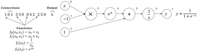
Figure 1. A sample CGP individual, with 3 inputs—$x,-1,1$—and 1 output—$y$. The genome consists of 5 3-valued genes, per 4 functional units, plus the output specification (no genes for the inputs). The first value of each 3-valued gene is the function’s index in the lookup table of functions (bottom-left), and the remaining two values are parameter nodes. The last gene determines the outputs to return. In the example above, with $n_{i}$ representing node $i$: node 3, gene 101, $f_{1}(n_{0},n_{1})=n_{0}\times n_{1}$; node 4, gene 330, $f_{3}(n_{3})=e^{n_{3}}$ (unary function, 3rd gene value ignored); node 5, gene 042, $f_{0}(n_{4},n_{2})=n_{4}+n_{2}$; node 6, gene 250, $f_{2}(n_{5})=\frac{1}{n_{5}}$; node 7, output node, $n_{6}$ is the designated output value. The topology is fixed throughout evolution, while the genome evolves.

The CGP library used in this paper (Quade, 2020) evolves the population in a $(1+\lambda)$-manner, i.e., in each generation it creates $\lambda$ offspring (we used the default $\lambda=4$) and compares their fitness to the parent individual. The fittest individual carries over to the next generation; in case of a draw, the offspring is preferred over the parent. Tournament selection is used, with tournament size $k=|population|$, single-point mutation, and no crossover. For more details, see (Miller and Smith, 2006; Quade, 2020). Table 3 delineates the hyperparameters used by the CGP algorithm, and Table 4 shows the primitive set.

Table 3. Hyperparameters used by CGP.

Parameter	Description	Value
operators	list of primitives	see Table 4
n_const	number of symbolic constants	0
n_rows	number of rows in the code block	5
n_columns	number of columns in the code block	5
n_back	number of rows to look back for connections	5
n_mutations	number of mutations per offspring	3
mutation_method	specific mutation method	point
max_iter	maximum number of generations	50
lambda	number of offspring per generation	4
f_tol	absolute error acceptable for convergence	0.01
n_jobs	number of jobs	1

Table 4. Set of primitives used by CGP. Left: Standard AFs. Right: Mathematical functions.

AF	Expression	AF	Expression
ReLU	$f(x)=max(x,0)$	Max	$f(x,y)=max(x,y)$
Tanh	$f(x)=\frac{e^{x}-e^{-x}}{e^{x}+e^{-x}}$	Min	$f(x,y)=min(x,y)$
Leaky ReLU	$f(x<0)=negative\_slope\cdot x$	Add	$f(x,y)=x+y$
	$f(x\geq 0)=x$
ELU	$f(x\leq 0)=(exp(x)-1)$	Sub	$f(x,y)=x-y$
	$f(x>0)=x$
HardShrink	$f(x<-\lambda)=x$	Mul	$f(x,y)=x\cdot y$
	$f(x>\lambda)=x$
	$f(-\lambda\leq x\leq\lambda)=0$
CELU	$f(x)=max(0,x)+min(0,\alpha(e^{\frac{x}{\alpha}}-1)$
Hardtanh	$f(x>1)=1$
	$f(x<-1)=-1$
	$f(-1\leq x\leq 1)=x$
Hardswish	$f(x\leq-3)=0$
	$f(x\geq 3)=-1$
	$f(-3<x\leq 3)=x\cdot\frac{(x+3)}{6}$
Softshrink	$f(x>\lambda)=x-\lambda$
	$f(x<-\lambda)=x+\lambda$
	$f(-\lambda\leq x\leq\lambda)=0$
RReLU	$f(x\geq 0)=x$
	$f(x<0)=\alpha\cdot x$
	($\alpha$ is uniformly, randomly sampled)

3.4. Evo-Single: Single-population evolution

Evo-Single is a single-population evolutionary algorithm, wherein an individual represents a single AF used throughout the whole network (as explained in Section 3.1). We start with the ReLU AF or the Leaky ReLU AF. Then we iterate, mutating the AF at every iteration of the CGP algorithm. Each individual is then trained over the train₁ set for 3 epochs and its fitness is computed as the accuracy over the train₂ set. After $\textit{max\_iter}*3=150$ iterations, we select the individual whose performance on the train₂ set was best. This individual is then compared against the other methods. The fitness-computation scheme is shown in Figure 2.

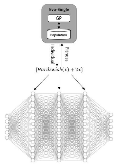
Figure 2. Evo-Single: Fitness computation of an individual in the population. The same AF is used throughout the network, in this example $Hardswish(x)+2x$.

3.5. Evo-Triple: Single-population evolution

Evo-Triple is a single-population evolutionary algorithm, wherein an individual comprises an array of 3 AFs, the first being the input-layer AF, the second being the hidden-layer AF, and the third being the output-layer AF. The AFs are used throughout the network as explained in Section 3.1. We start with 3 ReLU AFs or 3 Leaky ReLU AFs. Then we iterate, mutating each of the AFs at every iteration of the CGP algorithm. Each individual is then trained over the train₁ set for 3 epochs and its fitness is computed as the accuracy over the train₂ set. After $\textit{max\_iter}*3=150$ iterations, we select the individual whose performance on the train₂ set was best. This individual is than compared against the other methods. As with Evo-Single, training uses the train₁ set, and fitness is computed over the train₂ set. The fitness-computation scheme is shown in Figure 3.

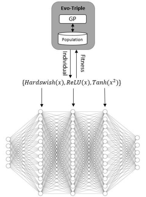
Figure 3. Evo-Triple: Fitness computation of an individual in the population, which comprises 3 AFs, in this example: $\{Hardswish(x),ReLU(x),Tanh(x^{2})\}$.

3.6. Coevo: Three-population coevolution

Coevolution refers to the simultaneous evolution of two or more species with coupled fitness (Pena-Reyes and Sipper, 2001). Coevolution can be mutualistic, parasitic, or commensalistic (Sipper et al., 2019). In mutualistic coevolution, two or more species reciprocally affect each other beneficially. Parasitic coevolution is a competitive relationship between species. Commensalistic coevolution is a relationship between species where one of the species gains benefits while the other neither benefits nor is harmed. In this paper we focus on mutualistic, or cooperative coevolution, which is based on the collaboration of several independently evolving species to solve a problem. An individual’s fitness is determined by its ability to cooperate with members of the other species.

Our coevolutionary algorithm comprises three separate populations: 1) input-layer AFs, 2) hidden-layer AFs, 3) output-layer AFs. Combining three individuals—one from each population—results in an AF architecture that can be evaluated. For each evolved individual in each population—an AF—we evaluated its fitness by choosing the two best (top-fitness) individuals of the two other populations from the previous generation. Each population evolved for $max\_iter=50$ iterations (generations). We then created a neural network composed of the three AFs in the respective input, hidden, and output layers. The scheme for fitness computation is depicted in Figure 4. As with Evo-Single and Evo-Triple, training uses the train₁ set, and fitness is computed over the train₂ set. The fitness-computation scheme is shown in Figure 4. The coevolutionary algorithm is described in Algorithm 1.

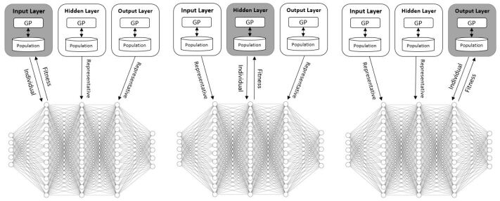
Figure 4. Fitness computation of an individual in Coevo requires cooperation from the other two populations.

Algorithm 1 Coevolutionary Algorithm: Main Components.

1:

2:function create_network(individual, best_input, best_hidden, best_output, $\mathit{pop}$)  $\#$ $\mathit{pop\in\{input,hidden,output\}}$

3:    if $\mathit{pop==input}$ then

4:         model $\leftarrow$ NeuralNetwork(individual, best_hidden, best_output)

5:    else if $\mathit{pop==hidden}$ then

6:         model $\leftarrow$ NeuralNetwork(best_input, individual, best_output)

7:    else $\#$ $\mathit{pop==output}$

8:         model $\leftarrow$ NeuralNetwork(best_input, best_hidden, individual)     return model

9:

10:function NeuralNetwork(input_af, hidden_af, output_af)

11:    model $\leftarrow$ Create a neural network with the given AFs, and input/output dimensions determined by dataset

12:    return model

13:

14:function fitness(model, train₁, train₂)

15:    train model for 3 epochs with cross entropy loss and mini-batches of size $|\mathit{train_{1}}|$/$10$

16:    return accuracy score over train₂

There might arise a concern over the differentiability of evolved AFs (PyTorch performs automatic differentiation—indeed this feature is one of its main strengths). However, in practice, this does not pose a problem since the number of points at which most functions are non-differentiable is usually (infinitely) small. For example, ReLU is non-differentiable at zero, however, in practice, it is rare to stumble often onto this value, and when we do, an arbitrary value can be assigned (e.g., zero), with little to no effect on performance. Our experiments have not shown differentiability to be of any concern.

4. Experimental Setup

We experimented with four supervised classification datasets—MNIST, FashionMNIST, KMNIST, USPS—using PyTorch’s (Paszke et al., 2019) default data loaders, with pixel values normalized between $[0,1]$ in the preprocessing step. The architectures used in the experiments are fixed and delineated in Tables 2 and 2. Full information about the datasets is shown in Table 5.

We used the Torchvision library—an accessible, open-source, machine-vision package for PyTorch, written in C++ (Marcel and Rodriguez, 2010). We used our GPU cluster, performing 20 replicate runs for each experimental setup. We split the data three ways into train₁ (60%, used to “locally” train the networks), train₂ (25%, used to “globally” evolve the networks), and test (15%) sets, using the training sets for the different automated approaches, while saving the test set for post-evaluation.

Table 5. Datasets. Note: 1 $\times$ $h$ $\times$ $w$ represents a single-channel (greyscale) image of height $h$ and width $w$.

Dataset	Images	Classes	Training	Test
MNIST	1 $\times$ 28 $\times$ 28	10	60,000	10,000
KMNIST	1 $\times$ 28 $\times$ 28	10	60,000	10,000
FashionMNIST	1 $\times$ 28 $\times$ 28	10	60,000	10,000
USPS	1 $\times$ 16 $\times$ 16	10	7291	2007

As noted above, we compared 5 different approaches: Standard-FCN/CNN, Random-FCN/CNN, Evo-Single, Evo-Triple, and Coevo. We ran multiple replicates of four kinds, each involving the execution and comparison of five different methods:

1. FCN, ReLU: Run Standard-FCN with ReLU, Random-FCN, Evo-Single, Evo-Triple, Coevo.

2. FCN, Leaky ReLU: Run Standard-FCN with Leaky ReLU, Random-FCN, Evo-Single, Evo-Triple, Coevo.

3. CNN, ReLU: Run Standard-CNN with ReLU, Random-CNN, Evo-Single, Evo-Triple, Coevo.

4. CNN, Leaky ReLU: Run Standard-CNN with Leaky ReLU, Random-CNN, Evo-Single, Evo-Triple, Coevo.

The score of a network at any given phase was its classification accuracy over said phase’s dataset. Scoring a standard network (either FCN or CNN) was done as follows: train the network using as training set both the train₁ and train₂ sets; the trained network’s final score for comparison purposes was its performance over the test set. Scoring the other types of networks (random, evolved, and coevolved) was done as follows: train the network using the train₁ set; use as fitness the score over the train₂ set; the network’s final score for comparison purposes was its performance over the test set. Note that the random and evolutionary algorithms never saw the test set—only the train₁ and train₂ sets were provided; solely the best individual returned was ascribed a test score based on the test set. In the next section, wherein we describe our results, values shown are test scores (i.e., over test sets).

Algorithm 2 delineates the experimental setup in pseudo-code format.

Algorithm 2 Experimental Setup

1:

2:

3:dataset $\leftarrow$ dataset to be used

4:replicates $\leftarrow$ number of replicates to run

5:

6:Performance measures (over test sets)

7:

8:for rep in {1…replicates} do

9:    Shuffle and split the dataset into train₁ set, train₂ set, test set

10:    Standard-Net $\leftarrow$ create a standard neural network  $\#$ Net is either FCN or CNN

11:    Random-Net $\leftarrow$ best network obtained through random search

12:    Evo-Single-Net $\leftarrow$ best network obtained through Evo-Single method

13:    Evo-Triple-Net $\leftarrow$ best network obtained through Evo-Triple method

14:    Coevo-Net $\leftarrow$ best network obtained through coevolution (Algorithm 1)

15:    for net in {Standard-Net, Random-Net, Evo-Single-Net, Evo-Triple-Net, Coevo-Net} do

16:         Train net on train₁ + train₂ sets for 30 epochs

17:         Test net on test set

18:         Record net’s test performance     

Figure 5 depicts an overview of the coevolutionary experimental setup. The code is available at https://github.com/razla.

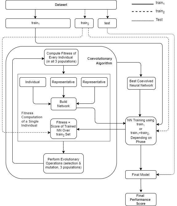
Figure 5. Overview of experimental coevolutionary setup. The coevolutionary algorithm uses the train₁ set to train a model and the train₂ set to evaluate the evolved model’s fitness. The train₁ and train₂ sets are combined together and used as the training set for the best coevolved neural network. The final model is tested over the test set.

5. Results and Analysis

Our experimental results are shown in Table 6. The mean of the highest per-replicate test accuracy score over all replicates, for each method, is reported as the best score for that method.

Table 6. Experimental results. Each line represents 20 replicates. Values shown are mean accuracy percentages over test set, where the mean is computed over best per-replicate scores for a particular method. The winning method is marked in boldface. Leaky: Leaky ReLU; Arch: Architecture.

Dataset	Baseline	Arch	Standard	Random	Evo-Single	Evo-Triple	Coevo
MNIST	ReLU	FCN	93.93	94.48	93.85	94.13	95.9
	Leaky	CNN	96.88	99.13	98.93	99.3	99.0
		FCN	94.98	93.68	93.53	95.7	95.5
		CNN	99.05	98.88	98.63	99.13	99.3
KMNIST	ReLU	FCN	80.3	80.58	80.88	81.33	80.15
	Leaky	CNN	59.58	95.15	94.78	94.68	94.8
		FCN	78.33	80.15	81.23	80.45	81.68
		CNN	94.7	93.98	93.15	95.38	94.23
FashionMNIST	ReLU	FCN	85.55	85.78	83.25	86.0	86.48
	Leaky	CNN	88.45	89.25	89.08	84.58	90.0
		FCN	86.25	85.58	83.13	86.43	85.68
		CNN	89.75	89.35	88.8	89.68	89.13
USPS	ReLU	FCN	90.52	91.27	91.39	84.91	91.4
	Leaky	CNN	89.1	96.13	93.77	95.39	96.01
		FCN	92.52	91.77	92.27	92.89	92.39
		CNN	96.38	95.39	94.39	96.01	96.88

Of the 16 groups of runs, Coevo won 7, Evo-Triple – 6, Random – 2, Standard – 1, and Evo-Single – 0 (wins are sometimes by a small margin but this is usual in this field). The standard FCN or CNN network was outperformed by the other methods in 15 out of the 16 groups of experiments, implying that automated AF search methods may increase model performance.

The fact that most wins involved 3 different AFs—either in Evo-Triple or in Coevo—affirms our surmise in Section 1: Combining different AFs improves network performance.

Table 7 presents the top-3 coevolved AF configurations for each of the four datasets. We note that some of the coevolved configurations are simpler and thus easier to use both for the feed-forward phase and the backpropagation phase. For brevity, we presented only the top-3 configurations, although there were many configurations that were composed only of simple evolved functions such as $x$, $2x$, and $x^{2}$.

Table 7. Coevolution: Top-3 AF configurations per dataset, per architecture. Each AF is of the form $f(x)=...$ with the $f(x)$ omitted for brevity. Each AF configuration is of the form {input-layer AF, hidden-layer AF, output-layer AF}.

MNIST
FCN	{$min(x,x^{2})-max(x^{2},\texttt{ReLU}(x))$, $\texttt{RReLU}(x)$, $\texttt{ELU}(x)$}
	{$x-max(x^{2},\texttt{ReLU}(x))$, $x$, $x$}
	{$x^{2}$, $\texttt{RReLU}(\texttt{RReLU}(\texttt{RReLU}(x)))$, $2x$}
CNN	{$x-\texttt{CELU}(x)$, $\texttt{Hardswish}(\texttt{ReLU}(x))$, $\texttt{RReLU}(\texttt{ReLU}(\texttt{Hardshrink}(x)))$}
	{$\texttt{Softshrink}(\texttt{Hardswish}(\texttt{Hardshrink}(x)))$, $\texttt{RReLU}(x)$, $\texttt{ReLU}(x)$}
	{$\texttt{Hardtanh}(x)-\texttt{CELU}(x)$, $\texttt{Hardswish}(\texttt{RReLU}(\texttt{ReLU}(x)))$, $\texttt{tanh}(x^{2})$}

KMNIST
FCN	{$\texttt{ELU}(\texttt{Hardswish}(x))$, $\texttt{CELU}(x)$, $\texttt{ReLU}(x)$}
	{$max(0,\texttt{ELU}(x))$, $x$, $\texttt{ELU}(x)$}
	{$\texttt{RReLU}(\texttt{ReLU}(\texttt{Hardshrink}(x)))$, $min(\texttt{Softshrink}(\texttt{ELU}(x)),x)$, $\texttt{ELU}(x)$
CNN	{$x$, $\texttt{Softshrink}(\texttt{Hardtanh}(x))$, $\texttt{RReLU}(x)-\texttt{Hardswish}(x)$}
	{$\texttt{Hardshrink}(x)$, $\texttt{Softshrink}(\texttt{Hardshrink}(x))$, $\texttt{LeakyRelu}(\texttt{tanh}(x^{2}))$}
	{$min((\texttt{Hardshrink}(x)*x),\texttt{ELU}(x))$, $\texttt{Softshrink}(\texttt{Hardtanh}(x))$, $\texttt{Hardtanh}(\texttt{Hardswish}(x))$}

FashionMNIST
FCN	{$\texttt{RReLU}(x)\cdot x+x$, $\texttt{ELU}(x)$, $2x$}
	{$x^{2}+x$, $max(\texttt{ReLU}(x),\texttt{LeakyRelu}(x)+2x)-(\texttt{LeakyRelu}(x)+2x)$, $2x$}
	{$\texttt{ELU}(max(\texttt{ReLU}(x),x))$, $\texttt{CELU}(\texttt{RReLU}(x))$, $\texttt{RReLU}(x)$}
CNN	{$\texttt{Hardswish}(x)$, $\texttt{RReLU}(x)$, $\texttt{ELU}(\texttt{LeakyRelu}(x)-x))$}
	{$\texttt{Hardswish}(x)$, $\texttt{Hardswish}(x)$, $\texttt{Softshrink}(\texttt{Softshrink}(\texttt{CELU}(x))$}
	{$\texttt{Softshrink}(x)$, $\texttt{Hardtanh}(\texttt{LeakyRelu}(\texttt{Hardswish}(x)))$, $\texttt{Hardtanh}(max(\texttt{Hardtanh}(\texttt{Hardswish}(x)),0)$}

USPS
FCN	{$\texttt{ELU}(\texttt{Hardswish}(x))$, $\texttt{CELU}(x)$, $\texttt{ReLU}(x)$}
	{$\texttt{Hardswish}(x)$, $x$, $\texttt{ELU}(x)$}
	{$\texttt{ReLU}(\texttt{CELU}(x))$, $\texttt{Hardswish}(\texttt{tanh}(x))+\texttt{RReLU}(x)$, $\texttt{LeakyReLU}(\texttt{ELU}(x))$}
CNN	{$\texttt{RReLU}(\texttt{tanh}(x))$, $\texttt{tanh}(x)$, $\texttt{LeakyReLU}(x)$}
	{$\texttt{HardSwish}(\texttt{Softshrink}(x))$, $\texttt{CELU}(\texttt{ELU}(x)-min(\texttt{LeakyReLU}(x),x))$, $min(\texttt{Hardshrink}(x)-x,\texttt{LeakyReLU}(x))$}
	{$\texttt{HardSwish}(\texttt{Softshrink}(x))$, $\texttt{ELU}(x)-min(\texttt{LeakyReLU}(x),x)$, $\texttt{Softshrink}(min(\texttt{Softshrink}(x),\texttt{Hardshrink}(x)-x))$}

6. Concluding Remarks

Despite the fact that deep-learning techniques are used for a wide range of applications, many hyperparameters must still be manually specified. The choice of AFs is a critical element that is often overlooked (i.e., standard AFs are used). We investigated the significance of AFs in learning in FCN and CNN models for image classification tasks. We introduced a coevolutionary algorithm to evolve new AFs and combine them beneficially, showing that our method performs well on four benchmark datasets.

We suggest a number of avenues for future research:

• Our focus herein was on classification tasks. Other deep-learning tasks can be examined too.

• During DNN learning, the influence of AFs on computational complexity could be analyzed.

• Applying coevolutionary technique to other DNN hyperparameter searches.

• Inspecting other DNN topologies, such as recurrent neural networks (RNNs) and autoencoders (AEs).

References

- (1)
- Agostinelli et al. (2014) Forest Agostinelli, Matthew Hoffman, Peter Sadowski, and Pierre Baldi. 2014. Learning activation functions to improve deep neural networks. arXiv preprint arXiv:1412.6830 (2014).
- Basirat and Roth (2018) Mina Basirat and Peter M Roth. 2018. The quest for the golden activation function. arXiv preprint arXiv:1808.00783 (2018).
- Bergstra and Bengio (2012) James Bergstra and Yoshua Bengio. 2012. Random search for hyper-parameter optimization. Journal of machine learning research 13, 2 (2012).
- Bingham et al. (2020) Garrett Bingham, William Macke, and Risto Miikkulainen. 2020. Evolutionary Optimization of Deep Learning Activation Functions. In Proceedings of the 2020 Genetic and Evolutionary Computation Conference (Cancún, Mexico) (GECCO ’20). Association for Computing Machinery, New York, NY, USA, 289–296.
- Bingham and Miikkulainen (2022) Garrett Bingham and Risto Miikkulainen. 2022. Discovering parametric activation functions. Neural Networks (2022).
- Breuel (2015) Thomas M Breuel. 2015. The effects of hyperparameters on SGD training of neural networks. arXiv preprint arXiv:1508.02788 (2015).
- Ding et al. (2022) Yadong Ding, Yu Wu, Chengyue Huang, Siliang Tang, Fei Wu, Yi Yang, Wenwu Zhu, and Yueting Zhuang. 2022. NAP: Neural Architecture search with Pruning. Neurocomputing (2022). https://doi.org/10.1016/j.neucom.2021.12.002
- Franchini et al. (2023) Giorgia Franchini, Valeria Ruggiero, Federica Porta, and Luca Zanni. 2023. Neural architecture search via standard machine learning methodologies. Mathematics in Engineering (2023). https://www.aimspress.com/article/doi/10.3934/mine.2023012?viewType=HTML
- Hochreiter (1998) Sepp Hochreiter. 1998. The vanishing gradient problem during learning recurrent neural nets and problem solutions. International Journal of Uncertainty, Fuzziness and Knowledge-Based Systems 6, 02 (1998), 107–116.
- Itano et al. (2018) Fernando Itano, Miguel Angelo de Abreu de Sousa, and Emilio Del-Moral-Hernandez. 2018. Extending MLP ANN hyper-parameters Optimization by using Genetic Algorithm. In 2018 International Joint Conference on Neural Networks (IJCNN). 1–8.
- Lu et al. (2019) Lu Lu, Yeonjong Shin, Yanhui Su, and George Em Karniadakis. 2019. Dying ReLU and initialization: Theory and numerical examples. arXiv preprint arXiv:1903.06733 (2019).
- Marcel and Rodriguez (2010) Sébastien Marcel and Yann Rodriguez. 2010. Torchvision the Machine-Vision Package of Torch. In Proceedings of the 18th ACM International Conference on Multimedia. Association for Computing Machinery, New York, NY, USA, 1485–1488.
- Miikkulainen et al. (2019) Risto Miikkulainen, Jason Liang, Elliot Meyerson, Aditya Rawal, Daniel Fink, Olivier Francon, Bala Raju, Hormoz Shahrzad, Arshak Navruzyan, Nigel Duffy, et al. 2019. Evolving deep neural networks. In Artificial intelligence in the age of neural networks and brain computing. Elsevier, 293–312.
- Miller and Harding (2008) Julian Francis Miller and Simon L. Harding. 2008. Cartesian Genetic Programming. In Proceedings of the 10th Annual Conference Companion on Genetic and Evolutionary Computation (Atlanta, GA, USA) (GECCO ’08). Association for Computing Machinery, New York, NY, USA, 2701–2726.
- Miller and Smith (2006) Julian F Miller and Stephen L Smith. 2006. Redundancy and computational efficiency in Cartesian genetic programming. IEEE Transactions on Evolutionary Computation 10, 2 (2006), 167–174.
- Miller et al. (1997) Julian F Miller, Peter Thomson, and Terence Fogarty. 1997. Designing electronic circuits using evolutionary algorithms. arithmetic circuits: A case study. Genetic Algorithms and Evolution Strategies in Engineering and Computer Science (1997), 105–131.
- Nader and Azar (2021) Andrew Nader and Danielle Azar. 2021. Evolution of Activation Functions: An Empirical Investigation. ACM Transactions on Evolutionary Learning and Optimization 1, 2 (2021), 1–36.
- Nwankpa et al. (2018) Chigozie Nwankpa, Winifred Ijomah, Anthony Gachagan, and Stephen Marshall. 2018. Activation functions: Comparison of trends in practice and research for deep learning. arXiv preprint arXiv:1811.03378 (2018).
- Paszke et al. (2019) Adam Paszke, Sam Gross, Francisco Massa, Adam Lerer, James Bradbury, Gregory Chanan, Trevor Killeen, Zeming Lin, Natalia Gimelshein, Luca Antiga, et al. 2019. PyTorch: An imperative style, high-performance deep learning library. Advances in neural information processing systems 32 (2019), 8026–8037.
- Pena-Reyes and Sipper (2001) Carlos Andrés Pena-Reyes and Moshe Sipper. 2001. Fuzzy CoCo: A cooperative-coevolutionary approach to fuzzy modeling. IEEE Transactions on Fuzzy Systems 9, 5 (2001), 727–737.
- Quade (2020) Markus Quade. 2020. cartesian. https://github.com/Ohjeah/cartesian.
- Saha et al. (2019) Snehanshu Saha, Nithin Nagaraj, Archana Mathur, and Rahul Yedida. 2019. Evolution of novel activation functions in neural network training with applications to classification of exoplanets. arXiv preprint arXiv:1906.01975 (2019).
- Sharma and Sharma (2017) Sagar Sharma and Simone Sharma. 2017. Activation functions in neural networks. Towards Data Science 6, 12 (2017), 310–316.
- Sipper (2021) Moshe Sipper. 2021. Neural Networks with À La Carte Selection of Activation Functions. SN Computer Science 2, 6 (2021), 1–9.
- Sipper et al. (2019) Moshe Sipper, Jason H Moore, and Ryan J Urbanowicz. 2019. Solution and fitness evolution (SAFE): Coevolving solutions and their objective functions. In European Conference on Genetic Programming. Springer, 146–161.
- Snoek et al. (2012) Jasper Snoek, Hugo Larochelle, and Ryan P Adams. 2012. Practical Bayesian optimization of machine learning algorithms. arXiv preprint arXiv:1206.2944 (2012).
- Stanley and Miikkulainen (2002) Kenneth O Stanley and Risto Miikkulainen. 2002. Evolving neural networks through augmenting topologies. Evolutionary computation 10, 2 (2002), 99–127.
- Sun et al. (2019) Yanan Sun, Bing Xue, Mengjie Zhang, and Gary G Yen. 2019. Evolving deep convolutional neural networks for image classification. IEEE Transactions on Evolutionary Computation 24, 2 (2019), 394–407.
- Wu et al. (2022) Meng-Ting Wu, Hung-I Lin, and Chun-Wei Tsai. 2022. A Training-Free Genetic Neural Architecture Search. In Proceedings of the 2021 ACM International Conference on Intelligent Computing and Its Emerging Applications (2022-01-01) (ACM ICEA ’21). Association for Computing Machinery, Jinan, China, 65–70. https://doi.org/10.1145/3491396.3506510
- Zhang et al. (2022) Haoyu Zhang, Yaochu Jin, Yaochu Jin, and Kuangrong Hao. 2022. Evolutionary Search for Complete Neural Network Architectures with Partial Weight Sharing. IEEE Transactions on Evolutionary Computation (2022), 1–1. https://doi.org/10.1109/TEVC.2022.3140855
- Zhang et al. (2017) Xiaohu Zhang, Yuexian Zou, and Wei Shi. 2017. Dilated convolution neural network with LeakyReLU for environmental sound classification. In 2017 22nd International Conference on Digital Signal Processing (DSP). IEEE, 1–5.
- Zhang et al. (2018) Yu-Dong Zhang, Chichun Pan, Junding Sun, and Chaosheng Tang. 2018. Multiple sclerosis identification by convolutional neural network with dropout and parametric ReLU. Journal of computational science 28 (2018), 1–10.