Functional Mixed Membership Models

Abstract

Mixed membership models, or partial membership models, are a flexible unsupervised learning method that allows each observation to belong to multiple clusters. In this paper, we propose a Bayesian mixed membership model for functional data. By using the multivariate Karhunen-Loève theorem, we are able to derive a scalable representation of Gaussian processes that maintains data-driven learning of the covariance structure. Within this framework, we establish conditional posterior consistency given a known feature allocation matrix. Compared to previous work on mixed membership models, our proposal allows for increased modeling flexibility, with the benefit of a directly interpretable mean and covariance structure. Our work is motivated by studies in functional brain imaging through electroencephalography (EEG) of children with autism spectrum disorder (ASD). In this context, our work formalizes the clinical notion of “spectrum” in terms of feature membership proportions. Supplementary materials, including proofs, are available online. The R package BayesFMMM is available to fit functional mixed membership models.

Keywords: Bayesian Methods, EEG, Functional Data, Mixed Membership Models, Neuroimaging

1 Introduction

Cluster analysis often aims to identify homogeneous subgroups of statistical units within a data set (Hennig et al., 2015). A typical underlying assumption of both heuristic and model-based procedures posits the existence of a finite number of sub-populations, from which each sample is extracted with some probability, akin to the idea of uncertain membership. A natural extension of this framework allows each observation to belong to multiple clusters simultaneously; leading to the concept of mixed membership models, or partial membership models (Blei et al., 2003; Erosheva et al., 2004), akin to the idea of mixed membership. This manuscript aims to extend the class of mixed membership models to functional data.

Functional data analysis (FDA) is concerned with the statistical analysis of the realizations of a random function. In the functional clustering framework, the random function is often conceptualized as a mixture of stochastic processes, so that each realization is assumed to be sampled from one of $K<\infty$ cluster-specific sub-processes. The literature on functional clustering is well established, and several analytical strategies have been proposed to handle different sampling designs and to ensure increasing levels of model flexibility (James and Sugar, 2003; Chiou and Li, 2007; Petrone et al., 2009; Jacques and Preda, 2014).

Beyond clustering, the ability to model an observation’s membership on a spectrum is particularly advantageous when we consider applications to biomedical data. For example, in diagnostic settings, the severity of symptoms may vary from person to person. Therefore, it is important to ask which symptomatic features characterize the sample and whether subjects exhibit one or more of these traits. Within this general context, our work is motivated by functional brain imaging studies of neurodevelopmental disorders, such as autism spectrum disorder (ASD). In this setting, typical patterns of neuronal activity are examined through the use of brain imaging technologies (e.g. electroencephalography (EEG)), and result in observations which are naturally characterized as random functions on a specific evaluation domain. We are primarily interested in the discovery of distinct functional features that characterize the sample and the explanation of how these features determine subject-level functional heterogeneity. To our knowledge, the literature on FDA is still silent on the concept of mixed membership, defining both the methodological and scientific need for a rigorous statistical formulation of functional mixed membership models. Figure 1 shows a conceptual illustration of the difference between data generated under the uncertain membership framework versus data generated under the mixed membership framework. In the mixed membership framework, components of the pure mixture can be continuously mixed to generate higher levels of realized heterogeneity in an observed sample.

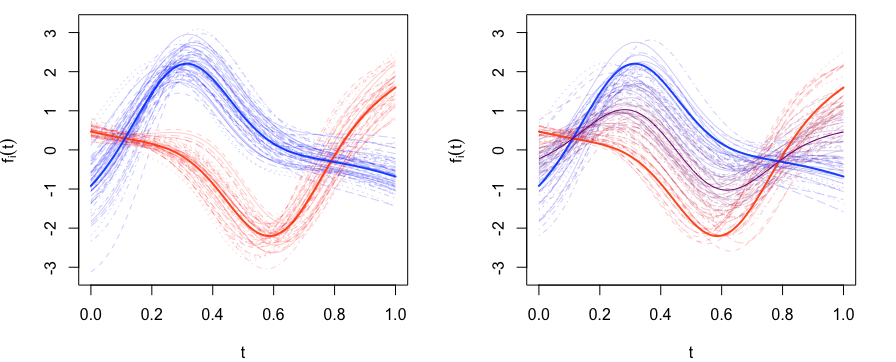
Figure 1: Generative model illustration. (Left panel) Data generated under the functional clustering framework. (Right panel) Data generated under a mixed membership framework.

One of the first uses of mixed membership models appeared in the field of population genetics. Pritchard et al. (2000) used the idea of mixed membership to group individuals into subpopulations, while accounting for the presence of admixed cases. Blei et al. (2003) introduced the concept of latent Dirichlet allocation to model mixed membership in the context of information retrieval associated with text corpora and other discrete data. These ideas have been extended to sampling models in the exponential family of distributions by Heller et al. (2008), and a general discussion of mixed versus partial membership models for continuous distributions is presented in Gruhl and Erosheva (2014). Prior distributions generalizing the concept of mixed membership to an arbitrary number of features have been discussed by Heller et al. (2008), who suggested leveraging the Indian buffet process (Griffiths and Ghahramani, 2011) to create a non-parametric mixed membership model. A comprehensive review and probabilistic generalizations of Bayesian clustering have been discussed by Broderick et al. (2013).

In this manuscript, we introduce the concept of mixed membership functions to the broader field of functional data analysis. Assuming a known number of latent functional features, we show how a functional mixed membership process is naturally defined through a simple extension of finite Gaussian process (GP) mixture models, by allowing mixing proportions to be indexed at the level of individual sample paths. Some sophistication is introduced through the multivariate treatment of the underlying functional features to ensure sampling models of adequate expressivity. Specifically, we represent a family of multivariate GPs through the multivariate Karhunen-Loève construction of Happ and Greven (2018). Using this idea, we jointly model the mean and covariance structures of the underlying functional features and derive a sampling model through the ensuing finite-dimensional marginal distributions. Since naïve GP mixture models assume that observations can only belong to one cluster, they only require the univariate treatment of the underlying GPs. However, when sample paths are allowed partial membership in multiple clusters, we need to assume independence between clusters or estimate the cross-covariance functions. Since the assumption of independence does not often hold in practice, we propose a model that allows us to jointly model the covariance and cross-covariance functions through the eigenfunctions of the multivariate covariance operator. Typically, this representation would require sampling on a constrained space to ensure that the eigenfunctions are mutually orthogonal. However, in this context, we are able to relax these constraints and maintain many of the desirable theoretical properties of our model by extending the multiplicative gamma process shrinkage prior proposed by Bhattacharya and Dunson (2011).

The remainder of the paper is organized as follows. Section 2 formalizes the concept of functional mixed membership as a natural extension of functional clustering. Section 3 discusses Bayesian inference through posterior simulation and establishes conditions for weak posterior consistency. Section 4 contains two simulation studies to assess operating characteristics on engineered data, and illustrates the application of the proposed model to a case study involving functional brain imaging through electroencephalography (EEG). Finally, we conclude our exposition with a critical discussion of the methodological challenges and related literature in Section 5.

2 Functional Mixed Membership

Functional data analysis (FDA) focuses on methods to analyze sample paths of an underlying continuous stochastic process $f:\mathcal{T}\rightarrow\mathbb{R}$, where $\mathcal{T}$ is a compact subset of $\mathbb{R}^{d}$. In the i.i.d. setting, a typical characterization of these stochastic processes relies on the definition of the mean function, $\mu(t)=\mathbb{E}\left(f(t)\right)$, and the covariance function, $C(s,t)=\text{Cov}\left(f(s),f(t)\right)$, where $t,s\in\mathcal{T}$. In this paper, we focus on jointly modeling $K$ underlying stochastic processes, where each stochastic process represents one cluster. In this section, we will proceed under the assumption that the number of clusters, $K$, is known a priori. While $K$ is fixed for the technical developments of the paper, Section 4.2 discusses the use of various information criteria for the selection of the optimal number of features.

Let $f^{(k)}_{clust}:\mathcal{T}\rightarrow\mathbb{R}$ denote the underlying stochastic process associated with the $k^{th}$ cluster. Let $\mu^{(k)}_{clust}$ and $C^{(k)}_{clust}$ be, respectively, the mean and covariance function corresponding to the $k^{th}$ stochastic process. To ensure desirable properties, such as decompositions, FDA often makes the assumption that the random functions are elements in a Hilbert space. Specifically, we assume $f^{(k)}_{clust}\in L^{2}(\mathcal{T})$ $\left(\int_{\mathcal{T}}|f^{(k)}(t)|^{2}\text{d}t<\infty\right)$. Within this context, a typical model-based representation of functional clustering assumes that each underlying process is a latent Gaussian process, $f^{(k)}_{clust}\sim\mathcal{GP}\left(\mu^{(k)}_{clust},C^{(k)}_{clust}\right)$, with sample paths $f_{i}$ $(i=1,2,\ldots,N)$, assumed to be independently drawn from a finite GP mixture

$$p\left(f_{i}\mid\rho^{(1:K)},\mu^{(1:K)}_{clust},C^{(1:K)}_{clust}\right)=\sum_{k=1}^{K}\rho^{(k)}\;\mathcal{GP}\left(f_{i}\mid\mu^{(k)}_{clust},C^{(k)}_{clust}\right);$$

where $\rho^{(k)}$ is the mixing proportion (fraction of sample paths) for component $k$, s.t. $\sum_{k=1}^{K}\rho^{(k)}=1$. Equivalently, by introducing latent variables $\tilde{\boldsymbol{\pi}}_{i}=\left(\tilde{\pi}_{i1},\ldots,\tilde{\pi}_{iK}\right)$, s.t. $\tilde{\boldsymbol{\pi}}_{i}\sim_{iid}\mbox{Multinomial}(1;\,\rho^{(1)},\ldots,\rho^{(K)})$, it is easy to show that,

$$f_{i}\mid\tilde{\boldsymbol{\pi}}_{1},\dots,\tilde{\boldsymbol{\pi}}_{N},\mu^{(1:K)}_{clust},C^{(1:K)}_{clust}\sim\mathcal{GP}\left(\sum_{k=1}^{K}\tilde{\pi}_{ik}\mu^{(k)}_{clust},\sum_{k=1}^{K}\tilde{\pi}_{ik}C^{(k)}_{clust}\right).$$ (1)

Mixed membership is naturally defined by generalizing the finite mixture model to allow each sample path to belong to a finite positive number of mixture components, which we call functional features (Heller et al., 2008; Broderick et al., 2013). Let $f^{(k)}$ denote the underlying Gaussian process associated with the $k^{th}$ functional feature where $\mu^{(k)}$ and $C^{(k)}$ denote the corresponding mean and covariance functions (note that $f^{(k)}$ need not be equal in distribution to $f^{(k)}_{clust}$). By introducing continuous latent variables $\mathbf{z}_{i}=(Z_{i1},\ldots,Z_{iK})^{\prime}$, where $Z_{ik}\in[0,1]$ and $\sum_{k=1}^{K}Z_{ik}=1$, the general form of the proposed mixed membership model follows the following convex combination:

$$f_{i}\mid\mathbf{z}_{1},\dots,\mathbf{z}_{N}=_{d}\sum_{k=1}^{K}Z_{ik}f^{(k)}.$$ (2)

In Equation 1, since each observation only belongs to one cluster, the Gaussian processes, $f^{(k)}_{clust}$, are most commonly assumed to be mutually independent. However, the same assumption is too restrictive for the model in Equation 2. Thus, we will let $C^{(k,k^{\prime})}$ denote the cross-covariance function between $f^{(k)}$ and $f^{(k^{\prime})}$, and denote with $\boldsymbol{\mathcal{C}}$ the collection of covariance and cross-covariance functions. Therefore, the sampling model for the proposed mixed membership scheme can be written as

$$f_{i}\mid\mathbf{z}_{1},\dots,\mathbf{z}_{N},\mu^{(1:K)},\boldsymbol{\mathcal{C}}\sim\mathcal{GP}\left(\sum_{k=1}^{K}Z_{ik}\mu^{(k)},\sum_{k=1}^{K}Z_{ik}^{2}C^{(k)}+\sum_{k=1}^{K}\sum_{k^{\prime}\neq k}Z_{ik}Z_{ik^{\prime}}C^{(k,k^{\prime})}\right).$$ (3)

Given a finite evaluation grid ${\bf t}_{i}=(t_{i1},\ldots,t_{in_{i}})^{\prime}$, the process’ finite-dimensional marginal distribution can be characterized s.t.

$$f_{i}({\bf t}_{i})\mid\mathbf{z}_{1},\dots,\mathbf{z}_{N},\mu^{(1:K)},\boldsymbol{\mathcal{C}}\sim\mathcal{N}\left(\sum_{k=1}^{K}Z_{ik}\mu^{(k)}({\bf t}_{i}),C_{i}({\bf t}_{i},{\bf t}_{i})\right),$$ (4)

where $C_{i}({\bf t}_{i},{\bf t}_{i})=\sum_{k=1}^{K}Z_{ik}^{2}C^{(k)}({\bf t}_{i},{\bf t}_{i})+\sum_{k=1}^{K}\sum_{k^{\prime}\neq k}Z_{ik}Z_{ik^{\prime}}C^{(k,k^{\prime})}({\bf t}_{i},{\bf t}_{i})$. A detailed comparison between our model and other similar models such as functional factor analysis models and FPCA can be found in Section B.3 of the Supplementary Materials. Since we do not assume that the functional features are independent, a concise characterization of the $K$ stochastic processes is needed in order to ensure that our model is scalable and computationally tractable. In Section 2.1, we review the multivariate Karhunen-Loève theorem (Happ and Greven, 2018), which will provide a joint characterization of the latent functional features, $\left(f^{(1)},f^{(2)},\ldots,f^{(K)}\right)$. Using this joint characterization, we are able to specify a scalable sampling model for the finite-dimensional marginal distribution found in Equation 4, which is described in full detail in Section 2.2.

2.1 Multivariate Karhunen-Loève Characterization

To aid in computation, we assume that $f^{(k)}$ is a smooth function and is in the $P$-dimensional subspace $\boldsymbol{\mathcal{S}}\subset L^{2}(\mathcal{T})$, spanned by a set of linearly independent square-integrable basis functions $\{b_{1},\dots,b_{P}\}$ ($b_{p}:\mathcal{T}\rightarrow\mathbb{R}$). While the choice of basis functions is user-defined, in practice B-splines (or the tensor product of B-splines for $\mathcal{T}\subset\mathbb{R}^{d}$ for $d\geq 2$) are a common choice due to their flexibility. De Boor (2000) has shown that for any smooth function, the distance between the true function and the approximation constructed using B-splines with uniform knots goes to zero as the number of knots goes to infinity. In practice, the number of basis functions used is often proportional to the average number of time points observed for each functional observation (Section E of the web-based appendix contains a detailed discussion on the choice of $P$). Alternative basis systems can be selected in relation to application-specific considerations.

The multivariate Karhunen-Loève (KL) theorem, proposed by Ramsay and Silverman (2005), can be used to jointly decompose our $K$ stochastic processes. To allow our model to handle higher-dimensional functional data, such as images, we will use the extension of the multivariate KL theorem for different dimensional domains proposed by Happ and Greven (2018). Although they state the theorem in full generality, we will only consider the case where $f^{(k)}\in\boldsymbol{\mathcal{S}}$. In this section, we will show that the multivariate KL theorem for different dimensional domains still holds under our assumption that $f^{(k)}\in\boldsymbol{\mathcal{S}}$, given that the conditions in Lemma 2.2 are satisfied.

We will start by defining the multivariate function $\mathbf{f}(\mathbf{t})$ in the following way:

$$\mathbf{f}(\mathbf{t}):=\left(f^{(1)}\left(t^{(1)}\right),f^{(2)}\left(t^{(2)}\right),\dots,f^{(K)}\left(t^{(K)}\right)\right),$$ (5)

where $\mathbf{t}$ is a $K$-tuple such that $\mathbf{t}=\left(t^{(1)},t^{(2)},\dots,t^{(K)}\right)$, where $t^{(1)},t^{(2)},\dots,t^{(K)}\in\mathcal{T}$. This construction allows for the joint representation of $K$ stochastic processes, each at different points in their domain. Since $f^{(k)}\in\boldsymbol{\mathcal{S}}$, we have $\mathbf{f}\in\boldsymbol{\mathcal{H}}:=\boldsymbol{\mathcal{S}}\times\boldsymbol{\mathcal{S}}\times\dots\times\boldsymbol{\mathcal{S}}:=\boldsymbol{\mathcal{S}}^{K}$. We define the corresponding mean of $\mathbf{f}(\mathbf{t})$, such that $\boldsymbol{\mu}(\mathbf{t}):=\left(\mu^{(1)}\left(t^{(1)}\right),\mu^{(2)}\left(t^{(2)}\right),\dots,\mu^{(K)}\left(t^{(K)}\right)\right)$, where $\boldsymbol{\mu}(\mathbf{t})\in\boldsymbol{\mathcal{H}}$, and the mean-centered cross-covariance functions as $C^{(k,k^{\prime})}(s,t):=\text{Cov}\left(f^{(k)}(s)-\mu^{(k)}(s),f^{(k^{\prime})}(t)-\mu^{(k^{\prime})}(t)\right)$, where $s,t\in\mathcal{T}$.

Lemma 2.1

$\boldsymbol{\mathcal{S}}$ is a closed linear subspace of $L^{2}(\mathcal{T})$.

Proofs for all results are given in the Supplementary Materials. From Lemma 2.1, since $\boldsymbol{\mathcal{S}}$ is a closed linear subspace of $L^{2}(\mathcal{T})$, we have that $\boldsymbol{\mathcal{S}}$ is a Hilbert space with respect to the inner product $\langle f,g\rangle_{\boldsymbol{\mathcal{S}}}=\int_{\mathcal{T}}f(t)g(t)\text{d}t$ where $f,g\in\boldsymbol{\mathcal{S}}$. By defining the inner product on $\boldsymbol{\mathcal{H}}$ as

$$\langle\mathbf{f},\mathbf{g}\rangle_{\boldsymbol{\mathcal{H}}}:=\sum_{k=1}^{K}\int_{\mathcal{T}}f^{(k)}\left(t^{(k)}\right)g^{(k)}\left(t^{(k)}\right)\text{d}t^{(k)},$$ (6)

where $\mathbf{f},\mathbf{g}\in\boldsymbol{\mathcal{H}}$, we have that $\boldsymbol{\mathcal{H}}$ is the direct sum of Hilbert spaces. Since $\boldsymbol{\mathcal{H}}$ is the direct sum of Hilbert spaces, $\boldsymbol{\mathcal{H}}$ is a Hilbert space (Reed and Simon, 1972). Thus, we have constructed a subspace $\boldsymbol{\mathcal{H}}$ using our assumption that $f^{(k)}\in\boldsymbol{\mathcal{S}}$, which satisfies Proposition 1 in Happ and Greven (2018). Letting $\mathbf{f}\in\boldsymbol{\mathcal{H}}$, we can define the covariance operator $\boldsymbol{\mathcal{K}}:\boldsymbol{\mathcal{H}}\rightarrow\boldsymbol{\mathcal{H}}$ element-wise in the following way:

$$\left(\boldsymbol{\mathcal{K}}\mathbf{f}\right)^{(k)}(\mathbf{t}):=\left\langle C^{(\cdot,k)}\left(\cdot,t^{(k)}\right),\mathbf{f}\right\rangle_{\boldsymbol{\mathcal{H}}}=\sum_{k^{\prime}=1}^{K}\int_{\mathcal{T}}C^{(k^{\prime},k)}\left(s,t^{(k)}\right)f^{(k^{\prime})}(s)\text{d}s.$$ (7)

Since we made the assumption $f^{(k)}\in\boldsymbol{\mathcal{S}}$, we can simplify Equation 7. Since $\boldsymbol{\mathcal{S}}$ is the span of the basis functions, we have $f^{(k)}(t)-\mu^{(k)}(t)=\sum_{p=1}^{P}\theta_{(k,p)}b_{p}(t)=\mathbf{B}^{\prime}(t)\boldsymbol{\theta}_{k},$ for some $\boldsymbol{\theta}_{k}\in\mathbb{R}^{P}$ and $\mathbf{B}^{\prime}(t)=[b_{1}(t)\cdots b_{P}(t)]$. Thus, we can see that

$$C^{(k,k^{\prime})}(s,t)=\text{Cov}\left(\mathbf{B}^{\prime}(s)\boldsymbol{\theta}_{k},\mathbf{B}^{\prime}(t)\boldsymbol{\theta}_{k^{\prime}}\right)=\mathbf{B}^{\prime}(s)\text{Cov}\left(\boldsymbol{\theta}_{k},\boldsymbol{\theta}_{k^{\prime}}\right)\mathbf{B}(t),$$ (8)

and we can rewrite Equation 7 as $\left(\boldsymbol{\mathcal{K}}\mathbf{f}\right)^{(k)}(\mathbf{t})=\sum_{k^{\prime}=1}^{K}\int_{\mathcal{T}}\mathbf{B}^{\prime}(s)\text{Cov}\left(\boldsymbol{\theta}_{k^{\prime}},\boldsymbol{\theta}_{k}\right)\mathbf{B}\left(t^{(k)}\right)f^{(k^{\prime})}(s)\text{d}s,$ for some $\mathbf{f}\in\mathcal{H}$. The following lemma establishes conditions under which $\boldsymbol{\mathcal{K}}$ is a bounded and compact operator, which is a necessary condition for the multivariate KL decomposition to exist.

Lemma 2.2

$\boldsymbol{\mathcal{K}}$ is a bounded and compact operator if we have that (1) the basis functions, $b_{1},\dots,b_{P}$, are uniformly continuous and (2) there exists $C_{max}\in\mathbb{R}$ such that $\left|\text{Cov}\left(\theta_{(k,p)},\theta_{(k^{\prime},p^{\prime})}\right)\right|\leq C_{max}$.

Assuming the conditions specified in lemma 2.2 hold, by the Hilbert-Schmidt theorem, since $\boldsymbol{\mathcal{K}}$ is a bounded, compact, and self-adjoint operator, we know that there exists real eigenvalues $\lambda_{1},\dots,\lambda_{KP}$ and a complete set of eigenfunctions $\boldsymbol{\Psi}_{1},\dots,\boldsymbol{\Psi}_{KP}\in\boldsymbol{\mathcal{H}}$ such that $\boldsymbol{\mathcal{K}}\boldsymbol{\Psi}_{p}=\lambda_{p}\boldsymbol{\Psi}_{p},$ for $p=1,\dots,KP.$ Since $\boldsymbol{\mathcal{K}}$ is a non-negative operator, we know that $\lambda_{p}\geq 0$ for $p=1,\dots,KP$ (Happ and Greven (2018), Proposition 2). From Theorem VI.17 of Reed and Simon (1972), we have that the positive, bounded, self-adjoint, and compact operator $\boldsymbol{\mathcal{K}}$ can be written as $\boldsymbol{\mathcal{K}}\mathbf{f}=\sum_{p=1}^{KP}\lambda_{p}\left\langle\boldsymbol{\Psi}_{p},\mathbf{f}\right\rangle_{\boldsymbol{\mathcal{H}}}\boldsymbol{\Psi}_{p}.$ Thus, from Equation 7, we have that

$$\sum_{k^{\prime}=1}^{K}\int_{\mathcal{T}}C^{(k^{\prime},k)}\left(s,t^{(k)}\right)f^{(k^{\prime})}(s)\text{d}s =\sum_{k^{\prime}=1}^{K}\int_{\mathcal{T}}\left(\sum_{p=1}^{KP}\lambda_{p}\Psi^{(k^{\prime})}_{p}(s)\Psi_{p}^{(k)}\left(t^{(k)}\right)\right)f^{(k^{\prime})}(s)\text{d}s,$$

where $\Psi_{p}^{(k)}(t^{(k)})$ is the $k^{th}$ element of $\boldsymbol{\Psi}_{p}(\mathbf{t})$. Thus, we can see that the covariance kernel can be written as the finite sum of eigenfunctions and eigenvalues,

$$C^{(k,k^{\prime})}(s,t)=\sum_{p=1}^{KP}\lambda_{p}\Psi^{(k)}_{p}(s)\Psi_{p}^{(k^{\prime})}(t).$$ (9)

Since we are working under the assumption that the random function, $\mathbf{f}\in\boldsymbol{\mathcal{H}}$, we can use a modified version of the Multivariate KL theorem. Considering that $\{\boldsymbol{\Psi}_{1},\dots,\boldsymbol{\Psi}_{KP}\}$ form a complete basis for $\boldsymbol{\mathcal{H}}$ and $\mathbf{f}(\mathbf{t})-\boldsymbol{\mu}(\mathbf{t})\in\boldsymbol{\mathcal{H}}$, we have

$$\mathbf{f}(\mathbf{t})-\boldsymbol{\mu}(\mathbf{t})\;=\;\mathbf{P}_{\boldsymbol{\mathcal{H}}}\circ\left(\mathbf{f}-\boldsymbol{\mu}\right)(\mathbf{t})\;=\;\sum_{p=1}^{KP}\left\langle\boldsymbol{\Psi}_{p},\mathbf{f}-\boldsymbol{\mu}\right\rangle_{\boldsymbol{\mathcal{H}}}\boldsymbol{\Psi}_{p}(\mathbf{t}),$$

where $\mathbf{P}_{\boldsymbol{\mathcal{H}}}$ is the projection operator onto $\boldsymbol{\mathcal{H}}$. Letting $\rho_{p}=\left\langle\boldsymbol{\Psi}_{p},\mathbf{f}-\boldsymbol{\mu}\right\rangle_{\boldsymbol{\mathcal{H}}}$, we have $\mathbf{f}(\mathbf{t})-\boldsymbol{\mu}(\mathbf{t})=\sum_{p=1}^{KP}\rho_{p}\boldsymbol{\Psi}_{p}(\mathbf{t})$, where $\mathbb{E}(\rho_{p})=0$ and $\text{Cov}(\rho_{p},\rho_{p^{\prime}})=\lambda_{p}\delta_{pp^{\prime}}$ (Happ and Greven, 2018).

Since $\boldsymbol{\Psi}_{p}\in\boldsymbol{\mathcal{H}}$ and $\boldsymbol{\mu}\in\boldsymbol{\mathcal{H}}$, there exist $\boldsymbol{\nu}_{k}\in\mathbb{R}^{P}$ and $\boldsymbol{\phi}_{kp}\in\mathbb{R}^{P}$ such that $\boldsymbol{\mu}^{(k)}(\mathbf{t})=\boldsymbol{\nu}_{k}^{\prime}\mathbf{B}\left(t^{(k)}\right)$ and $\sqrt{\lambda_{p}}\boldsymbol{\Psi}^{(k)}_{p}(\mathbf{t})=\boldsymbol{\phi}_{kp}^{\prime}\mathbf{B}\left(t^{(k)}\right):=\boldsymbol{\Phi}_{p}^{(k)}(\mathbf{t})$. These scaled eigenfunctions, $\boldsymbol{\Phi}_{p}^{(k)}(\mathbf{t})$, are used over $\boldsymbol{\Psi}^{(k)}_{p}(\mathbf{t})$ because they fully specify the covariance structure of the latent features, as described in Section 2.2. From a modeling prospective, the scaled eigenfunction parameterization is advantageous, as it admits a prior model based on the multiplicative gamma process shrinkage prior proposed by Bhattacharya and Dunson (2011), allowing for adaptive regularized estimation (Shamshoian et al., 2022). Thus we have

$$\mathbf{f}^{(k)}(\mathbf{t})=\boldsymbol{\mu}^{(k)}(\mathbf{t})+\sum_{p=1}^{KP}\chi_{p}\boldsymbol{\Phi}_{p}^{(k)}(\mathbf{t})=\boldsymbol{\nu}_{k}^{\prime}\mathbf{B}\left(t^{(k)}\right)+\sum_{p=1}^{KP}\chi_{p}\boldsymbol{\phi}_{kp}^{\prime}\mathbf{B}\left(t^{(k)}\right),$$ (10)

where $\chi_{p}=\left\langle(\lambda_{p})^{-1/2}\boldsymbol{\Psi}_{p},\mathbf{f}-\boldsymbol{\mu}\right\rangle_{\boldsymbol{\mathcal{H}}}$, $\mathbb{E}(\chi_{p})=0$, and $\text{Cov}(\chi_{p},\chi_{p^{\prime}})=\delta_{pp^{\prime}}$. Equation 10 gives us a way to jointly decompose any realization of the $K$ stochastic processes, $\mathbf{f}\in\boldsymbol{\mathcal{H}}$, as a finite weighted sum of basis functions.

Corollary 2.3

If $\chi_{p}\sim_{iid}\mathcal{N}(0,1)$, then the random function ${\bf f}(\mathbf{t})$ follows a multivariate $\mathcal{GP}$ with means $\boldsymbol{\mu}^{(k)}(\mathbf{t})=\boldsymbol{\nu}^{\prime}_{k}{\bf B}\left(t^{(k)}\right)$, and cross-covariance functions $C^{(k,k^{\prime})}(s,t)={\bf B}^{\prime}(s)\sum_{p=1}^{KP}(\boldsymbol{\phi}_{kp}\boldsymbol{\phi}^{\prime}_{k^{\prime}p}){\bf B}(t)$.

2.2 Functional Mixed Membership Process

In this section, we will describe a Bayesian additive model that allows for the constructive representation of mixed memberships for functional data. Our model allows for direct inference on the mean and covariance structures of the $K$ stochastic processes, which are often of scientific interest. To aid computational tractability, we will use the joint decomposition described in Section 2.1. In this section, we will assume that $f^{(k)}\in\boldsymbol{\mathcal{S}}$, and that the conditions of Lemma 2.2 hold.

We aim to model the mixed membership of $N$ observed sample paths, $\{\mathbf{Y}_{i}(.)\}_{i=1}^{N}$, to $K$ latent functional features ${\bf f}=\left(f^{(1)},f^{(2)},\ldots,f^{(K)}\right)$. Assuming that each path is observed at $n_{i}$ evaluation points ${\bf t}_{i}=[t_{i1}\cdots t_{in_{i}}]^{\prime}$, without loss of generality, we define a sampling model for the finite-dimensional marginals of ${\bf Y}_{i}({\bf t}_{i})$. To allow for path-specific partial membership, we extend the finite mixture model in Equation 1 and introduce path-specific mixing proportions $Z_{ik}\in(0,1)$, s.t. $\sum_{k=1}^{K}Z_{ik}=1$, for $i=1,2,\ldots,N$.

Let $\mathbf{S}(\mathbf{t}_{i})=[\mathbf{B}(t_{1})\cdots\mathbf{B}(t_{n_{i}})]\in\mathbb{R}^{P\times n_{i}}$, $\chi_{im}\sim\mathcal{N}(0,1)$, and $\boldsymbol{\Theta}$ denote the collection of model parameters. Let $M\leq KP$ be the number of eigenfunctions used to approximate the covariance structure of the $K$ stochastic processes. Using the decomposition of $f^{(k)}(t)$ in Equation 10 and assuming a normal distribution on ${\bf Y}_{i}({\bf t}_{i})$, we obtain:

$${\bf Y}_{i}({\bf t}_{i})|\boldsymbol{\Theta}\sim\mathcal{N}\left\{\sum_{k=1}^{K}Z_{ik}\left(\mathbf{S}^{\prime}(\mathbf{t}_{i})\boldsymbol{\nu}_{k}+\sum_{m=1}^{M}\chi_{im}\mathbf{S}^{\prime}({\bf t}_{i})\boldsymbol{\phi}_{km}\right),\;\sigma^{2}\mathbf{I}_{n_{i}}\right\}.$$ (11)

If we integrate out the latent $\chi_{im}$ variables, we obtain a more transparent form for the proposed functional mixed membership process. Specifically, we have

$$\mathbf{Y}_{i}(\mathbf{t}_{i})|\boldsymbol{\Theta}_{-\chi}\sim\mathcal{N}\left\{\sum_{k=1}^{K}Z_{ik}\mathbf{S}^{\prime}(\mathbf{t}_{i})\boldsymbol{\nu}_{k},\;\mathbf{V}_{i}+\sigma^{2}\mathbf{I}_{n_{i}}\right\},$$ (12)

where $\boldsymbol{\Theta}_{-\chi}$ is the collection of our model parameters excluding the $\chi_{im}$ variables, and $\mathbf{V}_{i}=\sum_{k=1}^{K}\sum_{k^{\prime}=1}^{K}Z_{ik}Z_{ik^{\prime}}\left\{\mathbf{S}^{\prime}(\mathbf{t}_{i})\sum_{m=1}^{M}\left(\boldsymbol{\phi}_{km}\boldsymbol{\phi}^{\prime}_{k^{\prime}m}\right)\mathbf{S}(\mathbf{t}_{i})\right\}.$ Thus, for a sample path, we have that the mixed membership mean is a convex combination of the functional feature means, and the mixed membership covariance, is a weighted sum of the covariance and cross-covariance functions between different functional features, following from the multivariate KL characterization in Section 2.1. Furthermore, from Equation 9 it is easy to show that, for large enough $M$, we have $\mathbf{S}^{\prime}(\mathbf{t}_{i})\sum_{m=1}^{M}\left(\boldsymbol{\phi}_{kp}\boldsymbol{\phi}^{\prime}_{k^{\prime}p}\right)\mathbf{S}(\mathbf{t}_{i})\approx C^{(k,k^{\prime})}(\mathbf{t}_{i},\mathbf{t}_{i}),$with equality when $M=KP$.

Mixed membership models can be thought of as a generalization of clustering. As such, these stochastic schemes are characterized by an inherent lack of likelihood identifiability. A typical source of non-indentifiability is the common label switching problem. To deal with the label switching problem, a relabelling algorithm can be derived for this model directly from the work of Stephens (2000). A second source of non-identifiabilty stems from allowing $Z_{ik}$ to be continuous random variables. Specifically, consider a model with 2 features and let $\boldsymbol{\Theta}_{0}$ be the set of “true” parameters. Let $Z_{i1}^{*}=0.5(Z_{i1})_{0}$ and $Z_{i2}^{*}=(Z_{i2})_{0}+0.5(Z_{i1})_{0}$. If we let $\boldsymbol{\nu}_{1}^{*}=2(\boldsymbol{\nu}_{1})_{0}-(\boldsymbol{\nu}_{2})_{0}$, $\boldsymbol{\nu}_{2}^{*}=(\boldsymbol{\nu}_{2})_{0}$, $\boldsymbol{\phi}_{1m}^{*}=2(\boldsymbol{\phi}_{1m})_{0}-(\boldsymbol{\phi}_{2m})_{0}$, $\boldsymbol{\phi}_{2m}^{*}=(\boldsymbol{\phi}_{2m})_{0}$, $\chi_{im}^{*}=(\chi_{im})_{0}$, and $(\sigma^{2})^{*}=\sigma^{2}_{0}$, we have $P(Y_{i}(t)|\boldsymbol{\Theta}_{0})=P(Y_{i}(t)|\boldsymbol{\Theta}^{*})$ (Equation 11). Thus, we can see that our model is not identifiable, and we will refer to this problem as the rescaling problem. To address the rescaling problem, additional assumptions such as the separability condition (Papadimitriou et al., 1998; McSherry, 2001; Azar et al., 2001; Chen et al., 2022) or the sufficiently scattered condition (Huang et al., 2016; Jang and Hero, 2019; Chen et al., 2022) are often made on the allocation parameters. The separability condition assumes that at least one observation belongs entirely to each feature, making it relatively easy to incorporate into a sampling model. To ensure that the separability condition holds in a two-feature model, we use the Membership Rescale Algorithm (Algorithm 2 in the Supplementary Materials). Compared to the separability condition, the sufficiently scattered condition makes weaker geometric assumptions on the sampling model when $K\geq 3$, but it is more difficult to implement in a sampling scheme. Section C.4 in the Supplementary Materials has an in-depth review of the two common assumptions made to address the rescaling problem.

A third non-identifiability problem may arise numerically as a form of concurvity, i.e. when $\boldsymbol{\nu}_{k^{\prime}}\propto\boldsymbol{\phi}_{km}$ in Equation 11. Typically, an overestimation of the magnitude of $\boldsymbol{\phi}_{km}$, may result in small variance estimates for the allocation parameters (smaller credible intervals). To address this problem, we can assume the separability condition; however, under weaker geometric assumptions this problem may persist, but is typically of little practical relevance.

2.3 Prior Distributions and Model Specification

The sampling model in Section 2.2, allows a practitioner to select how many eigenfunctions are to be used in the approximation of the covariance function. In the case of $M=KP$, we have a fully saturated model and can represent any realization $\mathbf{f}\in\boldsymbol{\mathcal{H}}$. In Equation 10, $\boldsymbol{\Phi}$ parameters are mutually orthogonal (where orthogonality is defined by the inner product defined in Equation 6), and have a magnitude proportional to the square root of the corresponding eigenvalue, $\lambda_{p}$. Thus, a modified version of the multiplicative gamma process shrinkage prior proposed by Bhattacharya and Dunson (2011) will be used as our prior for $\boldsymbol{\phi}_{km}$. By using this prior, we promote shrinkage across the $\boldsymbol{\phi}_{km}$ coefficient vectors, with increasing prior shrinkage towards zero as $m$ increases.

To facilitate MCMC sampling from the posterior target we will remove the assumption that $\boldsymbol{\Phi}$ parameters are mutually orthogonal. Even though $\boldsymbol{\Phi}$ parameters can no longer be thought of as scaled eigenfunctions, posterior inference can still be conducted on the eigenfunctions by post-processing posterior samples of $\boldsymbol{\phi}_{km}$ (given that we can recover the true covariance operator). Specifically, given posterior samples from $\boldsymbol{\phi}_{km}$, we obtain posterior realizations for the covariance function and then calculate the eigenpairs of the posterior samples of the covariance operator using the method described in Happ and Greven (2018). Thus, letting $\phi_{kpm}$ be the $p^{th}$ element of $\boldsymbol{\phi}_{km}$, we have

$$\phi_{kpm}|\gamma_{kpm},\tilde{\tau}_{mk}\sim\mathcal{N}\left(0,\gamma_{kpm}^{-1}\tilde{\tau}_{mk}^{-1}\right),\;\;\;\gamma_{kpm}\sim\Gamma\left(\nu_{\gamma}/2,\nu_{\gamma}/2\right),\;\;\;\tilde{\tau}_{mk}=\prod_{n=1}^{m}\delta_{nk},$$

$$\delta_{1k}|a_{1k}\sim\Gamma(a_{1k},1),\;\;\;\delta_{jk}|a_{2k}\sim\Gamma(a_{2k},1),\;\;\;a_{1k}\sim\Gamma(\alpha_{1},\beta_{1}),\;\;\;a_{2k}\sim\Gamma(\alpha_{2},\beta_{2}),$$

where $1\leq k\leq K$, $1\leq p\leq P$, $1\leq m\leq M$, and $2\leq j\leq M$. To promote shrinkage across the $M$ matrices, we need $\delta_{jk}>1$. Thus, letting $\alpha_{2}>\beta_{2}$, we have $\mathbb{E}(\delta_{jk})>1$, which will promote shrinkage. In this construction, we allow for different rates of shrinkage across different functional features, which is particularly important in cases where the covariance functions of different features have different magnitudes. In cases where the magnitudes of the covariance functions are different, we would expect $\delta_{mk}$ to be relatively smaller in the $k$ associated with the functional feature with a large covariance function.

To promote adaptive smoothing in the mean function, we will use a first-order random walk penalty proposed by Lang and Brezger (2004). The first-order random walk penalty penalizes differences in adjacent B-spline coefficients. In the case where $\mathcal{T}\subset\mathbb{R}$, we have that $P(\boldsymbol{\nu}_{k}|\tau_{k})\propto exp\left(-\frac{\tau_{k}}{2}\sum_{p=1}^{P-1}\left(\nu_{pk}^{\prime}-{\nu}_{(p+1)k}\right)^{2}\right),$ for $k=1,\dots,K$, where $\tau_{k}\sim\Gamma(\alpha,\beta)$ and $\nu_{pk}$ is the $p^{th}$ element of $\boldsymbol{\nu}_{k}$. Since we have $Z_{ik}\in(0,1)$ and $\sum_{k=1}^{K}Z_{ik}=1$, it is natural to consider prior Dirichlet sampling for $\mathbf{z}_{i}=[Z_{i1}\cdots Z_{iK}]$. Therefore, following Heller et al. (2008), we have

$$\mathbf{z}_{i}\mid\boldsymbol{\pi},\alpha_{3}\sim_{iid}Dir(\alpha_{3}\boldsymbol{\pi}),\;\;\;\boldsymbol{\pi}\sim Dir(\mathbf{c}),\;\;\;\alpha_{3}\sim Exp(b)$$

for $i=1,\dots,N$. Lastly, we will use a conjugate prior for our random error component of the model, such that $\sigma^{2}\sim IG(\alpha_{0},\beta_{0})$. Although we relax the assumption of orthogonality, in Section C.1 of the Supplementary Materials, we outline an alternative sampling scheme where we impose the condition that the $\boldsymbol{\Phi}$ parameters form orthogonal eigenfunctions using the work of Kowal et al. (2017).

3 Posterior Inference

Statistical inference is based on Markov chain Monte Carlo samples from the posterior distribution, by using the Metropolis-within-Gibbs algorithm. While the naïve sampling scheme is relatively simple, ensuring good exploration of the posterior target can be challenging due to the potentially multimodal nature of the posterior distribution. Specifically, some sensitivity of the results to the starting values of the chain can be observed for some data. Section C.2 of the Supplementary Materials outlines an algorithm for the selection of informed starting values. Furthermore, to mitigate sensitivity to chain initialization, we also implemented a tempered transition scheme, which improves the mixing of the Markov chain by allowing for transitions between modal configuration of the target. Implementation details for the proposed tempered transition scheme are reported in Section C.3 of the Supplementary Materials. Additional information on sampling schemes, as well as how to construct simultaneous confidence intervals, can be found in Section D of the Supplementary Materials.

3.1 Weak Posterior Consistency

In the previous section, we saw that the $\boldsymbol{\Phi}$ parameters are not assumed to be mutually orthogonal. By removing this constraint, we facilitate MCMC sampling from the posterior target and can perform inference on the eigenpairs of the covariance operator, as long as we can recover the covariance structure. Due to the complex identifiability issues mentioned in Section 2.2, establishing weak posterior consistency with unknown allocation parameters unattainable, even if we include the orthogonality constraint on the $\boldsymbol{\Phi}$ parameters. However, the model becomes identifiable when we condition on the allocation parameters. In this section, we show that we can achieve conditional weak posterior consistency without enforcing the orthogonality constraint of the $\boldsymbol{\Phi}$ parameter. Therefore, we will show that conditional on the allocation parameters, relaxing the orthogonality constraint does not affect our ability to recover the mean and covariance structure of the $K$ underlying stochastic processes from Equation 12. Let $\boldsymbol{\Pi}$ be the prior distribution on $\boldsymbol{\omega}:=\left\{\boldsymbol{\nu}_{1},\dots,\boldsymbol{\nu}_{K},\boldsymbol{\Sigma}_{11},\dots,\boldsymbol{\Sigma}_{1K},\dots,\boldsymbol{\Sigma}_{KK},\sigma^{2}\right\}$, where $\boldsymbol{\Sigma}_{kk^{\prime}}:=\sum_{p=1}^{KP}\left(\boldsymbol{\phi}_{kp}\boldsymbol{\phi}^{\prime}_{k^{\prime}p}\right)$. We will be proving weak posterior consistency with respect to the parameters $\boldsymbol{\Sigma}_{kk^{\prime}}$ because the parameters $\boldsymbol{\phi}_{kp}$ are non-identifiable. Since the covariance and cross-covariance structure are completely specified by the $\boldsymbol{\Sigma}_{kk^{\prime}}$ parameters, the lack of identifiability of the $\boldsymbol{\phi}_{kp}$ parameters bears no importance on inferential considerations. We will denote the true set of parameter values as $\boldsymbol{\omega}_{0}=\left\{(\boldsymbol{\nu}_{1})_{0},\dots,(\boldsymbol{\nu}_{K})_{0},(\boldsymbol{\Sigma}_{11})_{0},\dots,(\boldsymbol{\Sigma}_{1K})_{0},\dots,(\boldsymbol{\Sigma}_{KK})_{0},\sigma^{2}_{0}\right\}.$ To prove weak posterior consistency, we will make the following assumptions:

Assumption 1

Each sample path , $\mathbf{Y}_{i}$ ($i=1,\dots,N$), is observed at time points $\{t_{i1},\dots,t_{in_{i}}\}$, where $KP<n_{i}\leq n_{max}$ for some $n_{max}\in\mathbb{Z}^{+}$.

Assumption 2

The variables $Z_{ik}$ are known a-priori for $i=1,\dots,N$ and $k=1,\dots,K$.

Assumption 3

The true parameter that models random noise is positive ($\sigma^{2}_{0}>0$).

In order to prove weak posterior consistency, we will first specify the following quantities related to the Kullback–Leibler (KL) divergence. Following the notation of Choi and Schervish (2007), we define the following quantities:

$$\Lambda_{i}(\boldsymbol{\omega}_{0},\boldsymbol{\omega})=\text{log}\left(\frac{f_{i}(\mathbf{Y}_{i};\boldsymbol{\omega}_{0})}{f_{i}(\mathbf{Y}_{i};\boldsymbol{\omega})}\right),\;\;K_{i}(\boldsymbol{\omega}_{0},\boldsymbol{\omega})=\mathbb{E}_{\boldsymbol{\omega}_{0}}(\Lambda_{i}(\boldsymbol{\omega}_{0},\boldsymbol{\omega})),\;\;V_{i}(\boldsymbol{\omega}_{0},\boldsymbol{\omega})=\text{Var}_{\boldsymbol{\omega}_{0}}(\Lambda_{i}(\boldsymbol{\omega}_{0},\boldsymbol{\omega})),$$

where $f_{i}(\mathbf{Y}_{i};\boldsymbol{\omega}_{0})$ is the likelihood under $\boldsymbol{\omega}_{0}$. To simplify the notation, we define the following two quantities:

$$\boldsymbol{\mu}_{i} =\sum_{k=1}^{K}Z_{ik}\mathbf{S}^{\prime}(\mathbf{t})\boldsymbol{\nu}_{k},$$

$$\boldsymbol{\Sigma}_{i} =\sum_{k=1}^{K}\sum_{k^{\prime}=1}^{K}Z_{ik}Z_{ik^{\prime}}\left(\mathbf{S}^{\prime}(\mathbf{t})\sum_{p=1}^{KP}\left(\boldsymbol{\phi}_{kp}\boldsymbol{\phi}^{\prime}_{k^{\prime}p}\right)\mathbf{S}(\mathbf{t})\right)+\sigma^{2}\mathbf{I}_{n_{i}}=\mathbf{U}_{i}^{\prime}\mathbf{D}_{i}\mathbf{U}_{i}+\sigma^{2}\mathbf{I}_{n_{i}},$$

where $\mathbf{U}_{i}^{\prime}\mathbf{D}_{i}\mathbf{U}_{i}$ is the corresponding spectral decomposition. Let $d_{il}$ be the $l^{th}$ diagonal element of $\mathbf{D}_{i}$. Let $\boldsymbol{\Omega}_{\epsilon}(\boldsymbol{\omega}_{0})$ be the set of parameters such that the KL divergence is less than some $\epsilon>0$ ($\boldsymbol{\Omega}_{\epsilon}(\boldsymbol{\omega}_{0}):=\{\boldsymbol{\omega}:K_{i}(\boldsymbol{\omega}_{0},\boldsymbol{\omega})<\epsilon\text{ for all i}\}$). Let $a,b\in\mathbb{R}$ be such that $a>1$ and $b>0$, and define $\mathcal{B}(\boldsymbol{\omega}_{0}):=\left\{\boldsymbol{\omega}:\frac{1}{a}\left((d_{il})_{0}+\sigma^{2}_{0}\right)\leq d_{il}+\sigma^{2}\leq a\left((d_{il})_{0}+\sigma^{2}_{0}\right),\|\left(\boldsymbol{\mu}_{i}\right)_{0}-\boldsymbol{\mu}_{i}\|\leq b\right\}.$

Lemma 3.1

Let $\mathcal{C}(\boldsymbol{\omega}_{0},\epsilon):=\mathcal{B}(\boldsymbol{\omega}_{0})\cap\boldsymbol{\Omega}_{\epsilon}(\boldsymbol{\omega}_{0})$. Thus, for $\boldsymbol{\omega}_{0}\in\boldsymbol{\Omega}$ and $\epsilon>0$, there exist $a>1$ and $b>0$ such that (1) $\sum_{i=1}^{\infty}\frac{V_{i}(\boldsymbol{\omega}_{0},\boldsymbol{\omega})}{i^{2}}<\infty$, for any $\boldsymbol{\omega}\in\mathcal{C}(\boldsymbol{\omega}_{0},\epsilon)$ and (2) $\boldsymbol{\Pi}\left(\boldsymbol{\omega}\in\mathcal{C}(\boldsymbol{\omega}_{0},\epsilon)\right)>0$.

Lemma 3.1 shows that the prior probability of our parameters being arbitrarily close (defined by KL divergence) to the true parameters is positive. Since $\mathbf{Y}_{1},\dots,\mathbf{Y}_{N}$ are not identically distributed, condition (1) in Lemma 3.1 is necessary to prove Lemma 3.2.

Lemma 3.2

Under assumptions 1-3, the posterior distribution, $\boldsymbol{\Pi}_{N}(.|\mathbf{Y}_{1},\dots,\mathbf{Y}_{N})$, is weakly consistent at $\boldsymbol{\omega}_{0}\in\boldsymbol{\Omega}$.

All proofs are provided in the Supplementary Materials. Lemma 3.2 shows us that, conditional on the allocation parameters, we are able to recover the covariance structure of the $K$ stochastic processes. Thus, relaxation of the orthogonality constraint on the $\boldsymbol{\phi}_{km}$ parameters does not affect our ability to perform posterior inference on the main functions of scientific interest. Inference on the eigenstructure can still be performed by calculating the eigenvalues and eigenfunctions of the covariance operator using the MCMC samples of the $\boldsymbol{\phi}_{km}$ parameter. Finally, we point out that, in most cases, the parameters $Z_{ik}$ are unknown. Although theoretical guarantees for consistent estimation of the latent mixed allocation parameters are still elusive, we provide some empirical evidence of convergence in Section 4.1.

4 Case Studies and Experiments on Simulated Data

4.1 Simulation Study 1

In this simulation study, we examine how well our model can recover the mean and covariance functions when we vary the number of observed functions. The model used in this section is a mixed membership model with $2$ functional features ($K=2$), which can be represented by a basis constructed of $8$ B-splines ($P=8$), and uses $3$ eigenfunctions ($M=3$). We consider the case where we have $40$, $80$, and $160$ observed functional observations, where each observation is uniformly observed at $100$ time points. We then simulated 50 data sets for each of the three cases ($N=40,80,160$). To measure how well we recovered the the mean, covariance, and cross-covariance functions, we estimate the integrated relative mean square error (R-MISE), where $\text{R-MISE}=\frac{\int\{f(t)-\hat{f}(t)\}^{2}\text{d}t}{\int f(t)^{2}\text{d}t}\times 100\%$ and $\hat{f}$ is the estimated posterior median of the function $f$. To measure how well we recovered the allocation parameters, $Z_{ik}$, we calculated the root-mean-square error (RMSE). Section B.1 of the Supplementary Materials goes into more detail of how the model parameters were drawn, how estimates of all quantities of interest were calculated in this simulation, and includes visualizations of some of the recovered covariance structures.

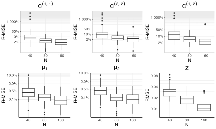
Figure 2: R-MISE values for the latent feature means and cross-covariances, as well as RMSE values for the allocation parameters, evaluated as sample size increases.

From Figure 2, we can see that we have a good recovery of the mean structure with as few as $40$ functional observations. While the R-MISE of the mean functions improves as we increase the number of functional observations ($N$), this improvement will likely have little practical impact. However, when looking at the recovery of the covariance and cross-covariance functions, we can see that the R-MISE noticeably decreases as more functional observations are added. As the recovery of the mean and covariance structures improves, the recovery of the allocation structure $(\mathbf{Z})$ improves. A supplementary simulation study examining how well our model can recover the mean, covariance, and allocation structures in a three-feature model ($K=3$) can be found in Section B.1 of the Supplementary Materials.

4.2 Simulation Study 2

Choosing the number of latent features can be challenging, especially when no prior knowledge is available for this quantity. Information criteria, such as the AIC, BIC, or DIC, are often used to aid practitioners in the selection of a data-supported value for $K$. In this simulation, we evaluate how various types of information criteria, as well as simple heuristics such as the “elbow-method”, perform in recovering the true number of latent features. To do this, we simulate 10 different data sets, each with 200 functional observations, from a mixed membership model with three functional features. We then calculate these information criteria on the 10 data sets for mixed membership models where $K=2,3,4,5$. Additional information on how the simulation study was conducted, as well as definitions of the information criterion, can be found in Section B.2 of the Supplementary Materials. As specified, the optimal model should have the largest BIC, the smallest AIC, and the smallest DIC.

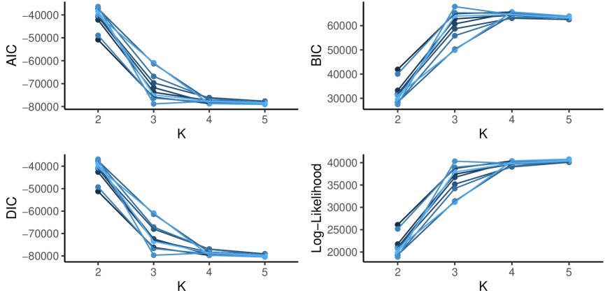
Figure 3: AIC, BIC, DIC, and the average log-likelihood evaluated for each of the 10 simulated data sets.

From the simulation results presented in Figure 3, we can see that on average each information criterion overestimated the number of functional features in the model. While the three information criteria seem to greatly penalize models that do not have enough features, they do not seem to punish overfit models to a great enough extent. As expected, the log-likelihood increases as we add more features; however, we can see that there is often an elbow at $K=3$ (Figure 3). Using the “elbow-method” led to selecting the correct number of latent functional features 8 times out of 10, while BIC picked the correct number of latent functional features twice. DIC and AIC were found to be the least reliable information criteria, only choosing the correct number of functional features once. Thus, through empirical consideration, we suggest using the “elbow-method” along with the BIC to aid in the final selection of the number of latent features to be interpreted in analyses. Although formal considerations of model-selection consistency are out of scope for the current contribution, we maintain that some of these techniques are best interpreted in the context of data exploration, with a potential for great improvement in interpretation if semi-supervised considerations allow for an a-priori informed choice of $K$.

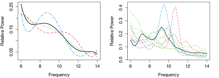
Figure 4: (Left Panel) Recovered means of model-based functional clustering with 4 clusters. (Right Panel) Alpha frequency patterns for a sample of EEG recordings from the T8 electrode of children (TD and ASD), styled by estimated cluster membership.

4.3 A Case Study of EEG in ASD

Autism spectrum disorder (ASD) is a term used to describe individuals with a collection of social communication deficits and restricted or repetitive sensory-motor behaviors (Lord et al., 2018). While once considered a very rare disorder with very specific symptoms, today the definition is more broad and is now thought of as a spectrum. Some individuals with ASD may have minor symptoms, while others may have very severe symptoms and require lifelong support. In this case study, we will use electroencephalogram (EEG) data that was previously analyzed by Scheffler et al. (2019) in the context of regression. The data set consists of EEG recordings of 39 typically developing (TD) children and 58 children with ASD between the ages of 2 and 12 years of age, which were analyzed in the frequency domain.

Scheffler et al. (2019) observed that the data from the T8 electrode, corresponding to the right temporal region, were correlated with ASD diagnosis, so we will specifically use the data from the T8 electrode in our mixed membership model. We focus our analysis to the alpha band of frequencies (6 to 14 Hz), whose patterns at rest are thought to play a role in neural coordination and communication between distributed brain regions. As clinicians examine the sample paths for the two cohorts, shown in Figure 4 (right panel), they are often interested in the location of a single prominent peak in the spectral density located within the alpha frequency band called the peak alpha frequency (PAF). This quantity has previously been associated with neural development in TD children (Rodríguez-Martínez et al., 2017). Scheffler et al. (2019) found that as TD children age, the peak becomes more prominent and the PAF shifts to a higher frequency. Conversely, a discernible PAF pattern is attenuated for most children with ASD compared to their TD counterpart.

A visual examination of the data in Figure 4 (right panel) anticipates the potential inadequacy of cluster analysis in this application, as path-specific heterogeneity does not seem to define well-separated subpopulations. In fact, if we cluster our data using the model in Pya Arnqvist et al. (2021) with $K=4$ (BIC selection), we find cluster means of dubious interpretability and poor separation of sample paths between clusters.

In contrast to classical clustering, we use a mixed membership model with only two functional features ($K=2$), (AIC-BIC selection). We note that the enhanced flexibility of mixed membership models induces parsimony in the number of pure mixture components supported by the data. In particular, the mean function of the first feature, depicted in Figure 5, can be interpreted as $1/f$ noise or pink noise. This component noise is expected to be found in every individual to some extent, but we can see that the first feature has no discernible alpha peak. The mean function of the second feature captures a distinct alpha peak, which is typically observed in EEGs of older neurotypical individuals. These two features help to differentiate between periodic (alpha waves) and aperiodic ($1/f$ trend) neural activity patterns, which coexist in the EEG spectrum. In this context, a model of uncertain membership would be necessarily inadequate to describe the heterogeneity of the observed sample path, as we would not naturally think of subjects in our sample as belonging to one or the other cluster. Instead, assuming mixed membership between the two-feature processes is likely to represent a more realistic data generating mechanism, as we conceptualize periodic and aperiodic neural activity patterns to mix continuously.

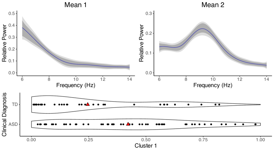
Figure 5: (Top Panel) Posterior median and 95% credible intervals (pointwise CI in dark gray and simultaneous CI in light gray) of the mean function for each functional feature. (Bottom Panel) Posterior median of each individual’s (feature-1)-membership, stratified by clinical cohort (cohort average (feature-1)-membership denoted by triangles).

Figure 5 shows that TD children are highly likely to heavily load feature 2 (well-defined PAF), whereas ASD children exhibit a higher level of heterogeneity. The cohort average (feature-1) membership, indicated by the triangles in Figure 5, shows that the average (feature-1)-membership for children with ASD is 0.42 compared to 0.25 for TD children. It is important to note that the allocation parameters constitute compositional data, meaning that using a Euclidean metric to measure mean membership may be inappropriate in cases where we have more than two features. Therefore, the use of Fréchet means (Fréchet, 1948) with a suitable metric for compositional data may be more appropriate to measure the centroids of the allocation parameters when we have more than two functional features. In general, these loadings suggest that clear alpha peaks take longer to emerge in children with ASD, compared to their typically developing counterparts.

In general, our findings confirm related evidence in the scientific literature on developmental neuroimaging but offer a completely novel point of view in quantifying group membership as part of a spectrum. Additional details on how the study was conducted, a posterior predictive check for a subset of individuals, and an in-depth comparison between our method and alternative methods such as FPCA and functional clustering are reported in Section B.3 of the Supplementary Materials. An extended analysis of multi-channel EEG for the same case study is reported in Section B.4 of the Supplementary Materials, investigating how spatial patterns vary across the scalp.

5 Discussion

This manuscript introduces the concept of functional mixed membership to the broader field of functional data analysis. Mixed membership is defined as a natural generalization of the concept of uncertain membership, which underlies the many approaches to functional clustering discussed in the literature. Our discussion is carried out within the context of Bayesian analysis. In this paper, a coherent and flexible sampling model is introduced by defining a mixed membership Gaussian process through projections on the linear subspace spanned by a suitable set of basis functions. Within this context, we leverage the multivariate KL formulation (Happ and Greven, 2018), to define a model ensuring weak conditional posterior consistency.

Our work is closely related to the approach introduced by Heller et al. (2008), who extended the theory of mixed membership models in the Bayesian framework for multivariate exponential family data. For Gaussian marginal distributions, their representation implies multivariate normal observations, with the natural parameters modeled as convex combinations of the individual cluster’s natural parameters. Although intuitively appealing, this idea has important drawbacks. Crucially, the differential entropy of observations in multiple clusters is constrained to be smaller than the minimum differential entropy across clusters, which may not be realistic in many sampling scenarios.

Information criteria are often used to aid the choice of $K$ in the context of mixture models. However, in Section 4.2, we saw that they often overestimated the number of features in our model. In simulations, we observed that using the “elbow-method” could lead to the selection of the correct number of features with good frequency. The literature has discussed non-parametric approaches to feature allocation models by using, for example, the Indian Buffet Processes (Griffiths and Ghahramani, 2011), but little is known about operating characteristics of these proposed procedures and little has been discussed about the ensuing need to carry out statistical inference across changing dimensions. Rousseau and Mengersen (2011), as well as Nguyen (2013), proved that under certain conditions, overfitted mixture models have a posterior distribution that converges to a set of parameters where the only components with positive weight will be the “true” parameters. However, by allowing the membership parameters to be a continuous random variable, we introduce a stronger type of nonidentifiability, which led to the rescaling problem discussed in Section 2.2. Therefore, more work is needed on the posterior convergence of overfitted models for mixed membership models.

6 Supplementary Materials

Supplementary Materials:

Contains proofs for all lemmas in the manuscript, as well as additional details for the case studies and simulation studies (BFMMM_Supplement.pdf).

BayesFMMM:

The R package to fit functional mixed membership models can be found on GitHub at https://github.com/ndmarco/BayesFMMM.

Simulation Studies and Case Studies:

The R scripts for the case studies and simulation studies can be found on GitHub at https://github.com/ndmarco/BFMMM_Functional_Sims. Unfortunately, the data for the EEG case study cannot be made publicly available.

References

- Azar et al. (2001) Azar, Y., Fiat, A., Karlin, A., McSherry, F. and Saia, J. (2001) Spectral analysis of data. In Proceedings of the thirty-third annual ACM symposium on Theory of computing, 619–626.
- Bhattacharya and Dunson (2011) Bhattacharya, A. and Dunson, D. B. (2011) Sparse bayesian infinite factor models. Biometrika, 291–306.
- Blei et al. (2003) Blei, D., Ng, A. and Jordan, M. (2003) Latent Dirichlet allocation. JMLR.
- Broderick et al. (2013) Broderick, T., Pitman, J. and Jordan, M. (2013) Feature allocations, probability functions, and paintboxes. Bayesian Analysis, 8, 801–836.
- Chen et al. (2022) Chen, Y., He, S., Yang, Y. and Liang, F. (2022) Learning topic models: Identifiability and finite-sample analysis. Journal of the American Statistical Association, 1–16.
- Chiou and Li (2007) Chiou, J.-M. and Li, P.-L. (2007) Functional clustering and identifying substructures of longitudinal data. Journal of the Royal Statistical Society: Series B (Statistical Methodology), 69, 679–699.
- Choi and Schervish (2007) Choi, T. and Schervish, M. J. (2007) On posterior consistency in nonparametric regression problems. Journal of Multivariate Analysis, 98, 1969–1987.
- De Boor (2000) De Boor, C. (2000) A practical guide to splines, vol. 27. New York: springer-verlag.
- Erosheva et al. (2004) Erosheva, E., Fienberg, S. and Lafferty, J. (2004) Mixed membership models of scientific publications. PNAS.
- Fréchet (1948) Fréchet, M. (1948) Les éléments aléatoires de nature quelconque dans un espace distancié. In Annales de l’institut Henri Poincaré, vol. 10, 215–310.
- Griffiths and Ghahramani (2011) Griffiths, T. and Ghahramani, Z. (2011) The Indian buffet process: An introduction and review. Journal of Machine Learning Research, 12, 1185–1224.
- Gruhl and Erosheva (2014) Gruhl, J. and Erosheva, E. (2014) A Tale of Two (Types of) Memberships: Comparing Mixed and Partial Membership with a Continuous Data Example, chap. 2. CRC Press.
- Happ and Greven (2018) Happ, C. and Greven, S. (2018) Multivariate functional principal component analysis for data observed on different (dimensional) domains. Journal of the American Statistical Association, 113, 649–659.
- Heller et al. (2008) Heller, K. A., Williamson, S. and Ghahramani, Z. (2008) Statistical models for partial membership. In Proceedings of the 25th International Conference on Machine learning, 392–399.
- Hennig et al. (2015) Hennig, C., Meila, M., Murtagh, F. and Rocci, r. (2015) Handbook of Cluster Analysis. CRC Press.
- Huang et al. (2016) Huang, K., Fu, X. and Sidiropoulos, N. D. (2016) Anchor-free correlated topic modeling: Identifiability and algorithm. Advances in Neural Information Processing Systems, 29.
- Jacques and Preda (2014) Jacques, J. and Preda, C. (2014) Model-based clustering for multivariate functional data. Computational Statistics & Data Analysis, 71, 92–106.
- James and Sugar (2003) James, G. M. and Sugar, C. A. (2003) Clustering for sparsely sampled functional data. Journal of the American Statistical Association, 98, 397–408.
- Jang and Hero (2019) Jang, B. and Hero, A. (2019) Minimum volume topic modeling. In The 22nd International Conference on Artificial Intelligence and Statistics, 3013–3021. PMLR.
- Kowal et al. (2017) Kowal, D. R., Matteson, D. S. and Ruppert, D. (2017) A bayesian multivariate functional dynamic linear model. Journal of the American Statistical Association, 112, 733–744.
- Lang and Brezger (2004) Lang, S. and Brezger, A. (2004) Bayesian p-splines. Journal of computational and graphical statistics, 13, 183–212.
- Lord et al. (2018) Lord, C., Elsabbagh, M., Baird, G. and Veenstra-Vanderweele, J. (2018) Autism spectrum disorder. The Lancet, 392, 508–520.
- McSherry (2001) McSherry, F. (2001) Spectral partitioning of random graphs. In Proceedings 42nd IEEE Symposium on Foundations of Computer Science, 529–537. IEEE.
- Nguyen (2013) Nguyen, X. (2013) Convergence of latent mixing measures in finite and infinite mixture models. The Annals of Statistics, 41, 370–400.
- Papadimitriou et al. (1998) Papadimitriou, C. H., Tamaki, H., Raghavan, P. and Vempala, S. (1998) Latent semantic indexing: A probabilistic analysis. In Proceedings of the seventeenth ACM SIGACT-SIGMOD-SIGART symposium on Principles of database systems, 159–168.
- Petrone et al. (2009) Petrone, S., Guindani, M. and Gelfand, A. E. (2009) Hybrid dirichlet mixture models for functional data. Journal of the Royal Statistical Society: Series B (Statistical Methodology), 71, 755–782.
- Pritchard et al. (2000) Pritchard, J. K., Stephens, M. and Donnelly, P. (2000) Inference of population structure using multilocus genotype data. Genetics, 155, 945–959.
- Pya Arnqvist et al. (2021) Pya Arnqvist, N., Arnqvist, P. and Sjöstedt de Luna, S. (2021) fdamocca: Model-based clustering for functional data with covariates. r package version 0.1-0.
- Ramsay and Silverman (2005) Ramsay, J. and Silverman, B. (2005) Principal components analysis for functional data. Functional data analysis, 147–172.
- Reed and Simon (1972) Reed, M. and Simon, B. (1972) Methods of modern mathematical physics, vol. 1. Elsevier.
- Rodríguez-Martínez et al. (2017) Rodríguez-Martínez, E., Ruiz-Martínez, F., Paulino, C. B. and Gómez, C. M. (2017) Frequency shift in topography of spontaneous brain rhythms from childhood to adulthood. Cognitive neurodynamics, 11, 23–33.
- Rousseau and Mengersen (2011) Rousseau, J. and Mengersen, K. (2011) Asymptotic behaviour of the posterior distribution in overfitted mixture models. Journal of the Royal Statistical Society: Series B (Statistical Methodology), 73, 689–710.
- Scheffler et al. (2019) Scheffler, A. W., Telesca, D., Sugar, C. A., Jeste, S., Dickinson, A., DiStefano, C. and Şentürk, D. (2019) Covariate-adjusted region-referenced generalized functional linear model for eeg data. Statistics in medicine, 38, 5587–5602.
- Shamshoian et al. (2022) Shamshoian, J., Senturk, D., Jeste, S. and Telesca, D. (2022) Bayesian analysis of longitudinal and multidimensional functional data. Biostatistics, 23, 558–573.
- Stephens (2000) Stephens, M. (2000) Dealing with label switching in mixture models. Journal of the Royal Statistical Society: Series B (Statistical Methodology), 62, 795–809.