Computationally Efficient PAC RL in POMDPs with Latent Determinism and Conditional Embeddings

Masatoshi Uehara mu223@cornell.edu Cornell University Ayush Sekhari as3663@cornell.edu Cornell University Jason D. Lee jasonlee@princeton.edu Princeton University Nathan Kallus kallus@cornell.edu Cornell University Wen Sun ws455@cornell.edu Cornell University
Abstract

We study reinforcement learning with function approximation for large-scale Partially Observable Markov Decision Processes (POMDPs) where the state space and observation space are large or even continuous. Particularly, we consider Hilbert space embeddings of POMDP where the feature of latent states and the feature of observations admit a conditional Hilbert space embedding of the observation emission process, and the latent state transition is deterministic. Under the function approximation setup where the optimal latent state-action $Q$-function is linear in the state feature, and the optimal $Q$-function has a gap in actions, we provide a computationally and statistically efficient algorithm for finding the exact optimal policy. We show our algorithmโ€™s computational and statistical complexities scale polynomially with respect to the horizon and the intrinsic dimension of the feature on the observation space. Furthermore, we show both the deterministic latent transitions and gap assumptions are necessary to avoid statistical complexity exponential in horizon or dimension. Since our guarantee does not have an explicit dependence on the size of the state and observation spaces, our algorithm provably scales to large-scale POMDPs.

1 Introduction

In reinforcement learning (RL), we often encounter partial observability of states [29]. Partial observability poses a serious challenge in RL from both computational and statistical aspects since observations are no longer Markovian. From a computational perspective, even if we know the dynamics, planning problems in POMDPs (partially observable Markov decision process) are known to be NP-hard [41]. From a statistical perspective, an exponential dependence on horizon in sample complexity is not avoidable without further assumptions [27].

We consider computationally and statistically efficient learning on large-scale POMDPs with deterministic transitions (but stochastic emissions). Here large-scale means that the POMDP might have large or even continuous state and observation spaces, but they can be modeled using conditional embeddings. Deterministic transitions and stochastic emissions is a very practically-relevant setting. For example, in robotic control, the dynamics of the robot itself is often deterministic but the observation of its current state is distorted by noise on the sensors [44, 43]. In human-robot-interaction, the robotsโ€™ dynamics is often deterministic, while humanโ€™s actions can be modeled as uncertain observations emitted from a distribution conditioned on robotโ€™s state and humanโ€™s pre-fixed goal [24]. For autonomous driving, the dynamics of the car in the 2d space is deterministic under normal road conditions, while the sensory data (e.g. GPS, IMU data, and Lidar scans) is modeled as stochastic. [4] offers further practical examples such as diagnosis of systems [42] and sensor management [25]. With known deterministic transitions, we can obtain positive results from computational perspectives for optimal planning [37, 5]. However, when transitions are unknown, learning algorithms that enjoy both computation and statistical efficiency are still limited to the tabular setting [27].

To design provably efficient RL algorithms for POMDPs with large state and observation spaces, we need to leverage function approximation. The key question that we aim to answer here is, under what structural conditions of the POMDPs, can we perform RL with function approximation with both statistical and computational efficiency? Specifically, we consider Hilbert space embeddings of POMDPs (HSE-POMDPs), where both features on the observations and latent states live in reproducing kernel Hilbert spaces (RKHSs), which are equipped with conditional embedding operators and the operators have non-zero singular values [7]. This assumption is similarly used in prior works such as learning HSE hidden Markov models [48] and HSE predictive state representations (HSE-PSRs) [6], where both have demonstrate that conditional embeddings are applicable to real-world applications such as estimating the dynamics of car from IMU data and estimating the configurations of a robot arm with raw pixel images. Also, HSE-POMDPs naturally capture undercomplete tabular POMDPs in [27]. For HSE-POMDPs with deterministic latent transition, we show positive results under the function approximation setting where the optimal $Q$-function over latent state and action is linear in the state feature, and the optimal $Q$-function has a non-trivial gap in the action space.

Our key contributions are as follows. Under the aforementioned setting, we propose an algorithm that learns the exact optimal policy with computational complexity and statistical complexity both polynomial in the horizon and intrinsic dimension (information gain) of the features. Notably, the complexity has no explicit dependence on the size of the problem including the sizes of the state and observation space, thus provably scaling to large-scale POMDPs. Our algorithm leverages a key novel finding that the linear optimal $Q$-function in the latent stateโ€™s feature together with the existence of the conditional embedding operator implies that the $Q$-functionโ€™s value can be estimated using new features constructed from the (possibly multiple-step) future observations, which are observable quantities. Our simple model-free algorithm operates completely using observable quantities and never tries to learn latent state transition and observation emission distribution, unlike existing works [39, 20, 3]. We also provide lower bounds indicating that in order to perform statistically efficient learning in POMDPs under linear function approximation, we need both the gap condition and the deterministic latent transition condition.

Computationally
Efficient
Deterministic
Transition
Non-tabular
Model-based or
Model-free
[20, 3, 27, 34] No No No Model-based
[9] No No Yes Model-based
[28] Yes Yes No Model-based
Our work Yes Yes Yes Model-free
Table 1: Summary of our work and existing works tackling statistically efficient learning on POMDPs. For details and additional works, refer to Sectionย 1.1. Note that deterministic transition does not preclude stochastic emissions and rewards.

1.1 Related Works

We here review and compare to related works. A summary is given in Tableย 1.

RL with linear $Q^{\star}$ in MDPs There is a large body of literature on online RL under the linear $Q^{\star}$-assumption with deterministic or nearly deterministic transitions [55, 16, 15]. The most relevant work is [15]. For a detailed comparison, refer to Remarkย 1.

Computational challenge in POMDPsโ€ƒThe seminal work [41] showed finding the optimal policy in POMPDPs is PSPACE-hard. Even worse, finding $\epsilon$-near optimal policy is PSPACE-hard, and finding the best memoryless policy is NP-hard [36, 8]. Recently [19] showed that quasi-polynomial time planning is attainable under the weak-observability assumption [18], which is similar to our assumption. However, their lower bound suggests that polynomial computation is still infeasible. Representative models that permit us to get polynomial complexity results are POMDPs where transitions are deterministic, but stochastic emissions [37, 4, 27]. We also consider deterministic latent transition with stochastic emission, but with function approximation.

Statistically efficient online learning in POMDPsโ€ƒ[17, 30] proposed algorithms that have $A^{H}$-type sample complexity, which is prohibitively large in the horizon. [20, 3, 56, 27, 39] show favorable sample complexities in the tabular setting using a model-based spectral learning framework [22]. [27] additionally showed a computationally and statistically efficient algorithm for tabular POMDPs with deterministic transitions. However, their algorithm crucially relies on the discreteness of the latent state space and it is unclear how to extend it to continuous settings. Also, our approach is model-free so does not need to model the emission process, which itself is an extremely challenging task when observations are high dimensional (e.g., raw-pixel images). In the no-ntabular setting, there are many works on learning uncontrolled dynamical systems in HSE-POMDPs [48, 6]. These existing works do not tackle the challenge of strategic exploration in online RL. Recent work [9] shows guarantees for related models in which the transition and observation dynamics are modeled by linear mixture models; however, their approach is computationally inefficient. We remark there are further works tackling online RL in other POMDPs, such as LQG [33, 46], latent POMDPs [32] and reactive POMDPs [31, 26].

2 Preliminaries

We first introduce POMDPs, HSE-POMDPs, and our primary assumptions.

2.1 Partially Observable Markov Decision Processes

We consider an episodic POMDP given by the tuple (H,๐’ฎ,๐’œ,๐’ช,๐•‹,๐•†,๐•,s0)๐ป๐’ฎ๐’œ๐’ช๐•‹๐•†๐•subscript๐‘ 0(H,{\mathcal{S}},\mathcal{A},\mathcal{O},\mathbb{T},\mathbb{O},\mathbb{Y},s_{0}). Here, $H$ is the number of steps in each episode, ${\mathcal{S}}$ is the set of states, $\mathcal{A}$ is the set of actions with $|\mathcal{A}|=A$, $\mathcal{O}$ is the set of observations, $\mathbb{T}=\{\mathbb{T}_{h}\}_{h=0}^{H-1}$ is the transition dynamics such that $\mathbb{T}_{h}$ is a map from ${\mathcal{S}}\times\mathcal{A}$ to $\Delta(\mathcal{A})$, $\mathbb{O}=\{\mathbb{O}_{h}\}_{h=0}^{H-1}$ is the set of emission distributions such that $\mathbb{O}_{h}$ is a map from ${\mathcal{S}}$ to $\Delta(\mathcal{O})$, $\mathbb{Y}=\{\mathbb{Y}_{h}\}_{h=0}^{H-1}$ is the set of reward distributions such that $\mathbb{Y}_{h}$ is a map from ${\mathcal{S}}\times\mathcal{A}$ to $\Delta(\mathbb{R})$, and s0subscript๐‘ 0s_{0} is a fixed initial state. We denote the conditional mean of the reward distribution by $r_{h}:{\mathcal{S}}\times\mathcal{A}\to\mathbb{R}$ and the noise by $\tau$, so that rhโ€‹(s,a)+ฯ„subscript๐‘Ÿโ„Ž๐‘ ๐‘Ž๐œr_{h}(s,a)+\tau has law ๐•hโ€‹(s,a)subscript๐•โ„Ž๐‘ ๐‘Ž\mathbb{Y}_{h}(s,a). We suppose that ๐•hโ€‹(s,a)subscript๐•โ„Ž๐‘ ๐‘Ž\mathbb{Y}_{h}(s,a) lies in $[0,1]$.

In a POMDP, states are not observable to agents. Each episode starts from s0subscript๐‘ 0s_{0} at $h=0$. At each step $h\in[H]$, the agent observes $o_{h}\in\mathcal{O}$ generated from the hidden state shโˆˆ๐’ฎsubscript๐‘ โ„Ž๐’ฎs_{h}\in{\mathcal{S}} following $\mathbb{O}_{h}(\cdot\mid s_{h})$, the agent picks an action $a_{h}\in\mathcal{A}$, receives a reward $r_{h}$ following $\mathbb{Y}_{h}(\cdot\mid s,a)$, and then transits to the next latent state $s_{h+1}\sim\mathbb{T}_{h}(\cdot|s_{h},a_{h})$.

We streamline the notation as follows. We let $o_{0:h}$ denote $o_{0},\ldots,o_{h}$, and similarly for $a_{0:h}$. Given a matrix $A$, let $\eta(A)$ be its smallest singular value. Given a vector $a$ and matrix $A$, let $\|a\|^{2}_{A}=a^{\top}Aa$. Give vectors $a$ and $b$, we define $\langle a,b\rangle=a^{\top}b$.

2.2 Hilbert Space Embedding POMDPs

We introduce our model, HSE-POMDPs. For ease of presentation, we first focus on the finite-dimensional setting with 1-step observability, i.e., using one-step future observation for constructing the conditional mean embedding. We extend to infinite-dimensional RKHS in Sectionย B. We extend to multiple-step future observations in Sectionย 5.

Consider two features, one on the observation, $\psi:\mathcal{O}\to\mathbb{R}^{d}$, and one on latent state, ฯ•:๐’ฎโ†’โ„ds:italic-ฯ•โ†’๐’ฎsuperscriptโ„subscript๐‘‘๐‘ \phi:{\mathcal{S}}\to\mathbb{R}^{d_{s}}.

Assumption 1 (Existence of linear conditional mean embedding and left invertibility).

Assume for any $h\in[H]$, there exists a left-invertible matrix Ghโˆˆโ„dร—dssubscript๐บโ„Žsuperscriptโ„๐‘‘subscript๐‘‘๐‘ G_{h}\in\mathbb{R}^{d\times d_{s}} such that ๐”ผoโˆผ๐•†hโ€‹(s)โ€‹[ฯˆโ€‹(o)]=Ghโ€‹ฯ•โ€‹(s)subscript๐”ผsimilar-to๐‘œsubscript๐•†โ„Ž๐‘ delimited-[]๐œ“๐‘œsubscript๐บโ„Žitalic-ฯ•๐‘ \mathbb{E}_{o\sim\mathbb{O}_{h}(s)}[\psi(o)]=G_{h}\phi(s), and โˆƒGhโ€ โˆˆโ„dsร—dsuperscriptsubscript๐บโ„Žโ€ superscriptโ„subscript๐‘‘๐‘ ๐‘‘\exists G_{h}^{\dagger}\in\mathbb{R}^{d_{s}\times d} such that Ghโ€ โ€‹Gh=Isuperscriptsubscript๐บโ„Žโ€ subscript๐บโ„Ž๐ผG_{h}^{\dagger}G_{h}=I.

The left invertible condition is equivalent to saying that $G_{h}$ is full column rank (it also requires that dโ‰ฅds๐‘‘subscript๐‘‘๐‘ d\geq d_{s}). This assumption is widely used in the existing literature on learning uncontrolled partially observable systems [48, 49, 6]. We permit the case where ds=โˆž,d=โˆžformulae-sequencesubscript๐‘‘๐‘ ๐‘‘d_{s}=\infty,d=\infty as later formalized in Sectionย B. We present two concrete examples below.

Example 1 (Undercomplete tabular POMDPs).

Let ds=|๐’ฎ|subscript๐‘‘๐‘ ๐’ฎd_{s}=|{\mathcal{S}}| and $d=|\mathcal{O}|$, define $\phi$ and $\psi$ as one-hot encoding vectors over ${\mathcal{S}}$ and $\mathcal{O}$, respectively. We overload notation and denote ๐•†hโˆˆโ„dร—dssubscript๐•†โ„Žsuperscriptโ„๐‘‘subscript๐‘‘๐‘ \mathbb{O}_{h}\in\mathbb{R}^{d\times d_{s}} as a matrix with entry $(i,j)$ equal to ๐•†hโ€‹(o=i|s=j)subscript๐•†โ„Ž๐‘œconditional๐‘–๐‘ ๐‘—\mathbb{O}_{h}(o=i|s=j). This $\mathbb{O}_{h}$ corresponds to $G_{h}$. Assumption 1 is satisfied if $\mathbb{O}_{h}$ is full column rank. This assumption is used in [22] for learning tabular undercomplete HMMs. We discuss the overcomplete case $|\mathcal{O}|\leq|{\mathcal{S}}|$ in Sectionย 5.

Example 2 (Gaussian POMDPs with discrete latent states [38]).

Suppose ${\mathcal{S}}$ is discrete but $\mathcal{O}$ is continuous, and $\mathbb{O}_{h}(\cdot\mid s)=\mathcal{N}(\mu_{s,h},I)$. Then, letting $O_{h}=[\mu_{1:h},\cdots,\mu_{|{\mathcal{S}}|:h}]\in\mathbb{R}^{d\times|{\mathcal{S}}|}$ and $\phi(\cdot)$ be a one-hot encoding vector over ${\mathcal{S}}$, we have $\mathbb{E}_{o\sim\mathbb{O}_{h}(\cdot\mid s)}[o]=O_{h}\phi(s)$. Assumption 1 is satisfied when $O_{h}$ is full-column rank, i.e., the means of the Gaussian distributions are linearly independent.

2.3 Assumptions and function approximation

We introduce three additional assumptions: deterministic transitions, linear $Q^{\star}$, and the existence of an optimality gap. The first assumption is as follows.

Assumption 2 (Systems with deterministic state transitions).

The transition dynamics $\mathbb{T}_{h}$ is deterministic, i.e., there exists a mapping $p_{h}:{\mathcal{S}}\times\mathcal{A}\to{\mathcal{S}}$ such that $\mathbb{T}_{h}(\cdot\mid s,a)$ is Dirac at phโ€‹(s,a)subscript๐‘โ„Ž๐‘ ๐‘Žp_{h}(s,a).

Notice Assumption 2 ensures the globally optimal policy $\pi^{\star}=\mathop{\mathrm{argmax}}_{\pi}\mathbb{E}_{\pi}[\sum_{h}r_{h}]$ is given as a sequence of (non-history-dependent and deterministic) actions $a^{\star}_{0:H-1}$.

Here, we stress three points. First, rewards and emission probabilities can still be stochastic. Second, Assumption 2 is standard in the literature on MDPs [55, 31, 15] and POMDPs [5, 37] . As mentioned in Sectionย 1, this setting is practical in many real-world applications. Third, while we can consider learning about POMDPs with stochastic transitions, even if we know the transitions and focus on planning, computing a near-optimal policy is PSPACE-hard [41]. This implies we must need additional conditions. Deterministic transitions can be regarded as one such possible condition, in particular one that is relevant to many real-world applications.

Next, we suppose the optimal latent $Q$-function is linear in the state feature. Given a level $h\in[H]$ and state-action pair (s,a)โˆˆ๐’ฎร—๐’œ๐‘ ๐‘Ž๐’ฎ๐’œ(s,a)\in{\mathcal{S}}\times\mathcal{A}, the optimal $Q$-function on the latent state is recursively defined as Qhโ‹†โ€‹(s,a)=rโ€‹(s,a)+maxaโ€ฒโกQh+1โ‹†โ€‹(phโ€‹(s,a),aโ€ฒ)subscriptsuperscript๐‘„โ‹†โ„Ž๐‘ ๐‘Ž๐‘Ÿ๐‘ ๐‘Žsubscriptsuperscript๐‘Žโ€ฒsubscriptsuperscript๐‘„โ‹†โ„Ž1subscript๐‘โ„Ž๐‘ ๐‘Žsuperscript๐‘Žโ€ฒQ^{{\star}}_{h}(s,a)=r(s,a)+\max_{a^{\prime}}Q^{\star}_{h+1}(p_{h}(s,a),a^{\prime}) starting from QHโ‹†โ€‹(s,a)=0,โˆ€s,asubscriptsuperscript๐‘„โ‹†๐ป๐‘ ๐‘Ž0for-all๐‘ ๐‘ŽQ^{\star}_{H}(s,a)=0,\forall s,a. We define Vhโ‹†โ€‹(s)=maxaโกQhโ‹†โ€‹(s,a)subscriptsuperscript๐‘‰โ‹†โ„Ž๐‘ subscript๐‘Žsubscriptsuperscript๐‘„โ‹†โ„Ž๐‘ ๐‘ŽV^{{\star}}_{h}(s)=\max_{a}Q^{{\star}}_{h}(s,a). Now we are ready to introduce the linearity assumption.

Assumption 3 (Linear $Q^{\star}$).

Given the state feature ฯ•:๐’ฎโ†’โ„ds:italic-ฯ•โ†’๐’ฎsuperscriptโ„subscript๐‘‘๐‘ \phi:{\mathcal{S}}\to\mathbb{R}^{d_{s}}, for any $h\in[H]$ and any $a\in[A]$, there exists wa;hโ‹†โˆˆโ„dssubscriptsuperscript๐‘คโ‹†๐‘Žโ„Žsuperscriptโ„subscript๐‘‘๐‘ w^{\star}_{a;h}\in\mathbb{R}^{d_{s}} such that Qhโ‹†โ€‹(s,a)=โŸจwa;hโ‹†,ฯ•โ€‹(s)โŸฉsubscriptsuperscript๐‘„โ‹†โ„Ž๐‘ ๐‘Žsubscriptsuperscript๐‘คโ‹†๐‘Žโ„Žitalic-ฯ•๐‘ Q^{\star}_{h}(s,a)=\langle w^{\star}_{a;h},\phi(s)\rangle for any sโˆˆ๐’ฎ๐‘ ๐’ฎs\in{\mathcal{S}} and $\|w^{\star}_{a;h}\|\leq W$.

This assumption is widely used in RL [16, 15, 34, 14]. We further consider the infinite-dimensional case in Sectionย B.

Next, we assume an optimality gap. For any $h\in[H]$, define gaphโ€‹(s,a)=Vhโ‹†โ€‹(s)โˆ’Qhโ‹†โ€‹(s,a)subscriptgapโ„Ž๐‘ ๐‘Žsubscriptsuperscript๐‘‰โ‹†โ„Ž๐‘ subscriptsuperscript๐‘„โ‹†โ„Ž๐‘ ๐‘Ž\mathrm{gap}_{h}(s,a)=V^{\star}_{h}(s)-Q^{\star}_{h}(s,a).

Assumption 4 (Optimality Gap).

min(h,s,a)โก{gaphโ€‹(s,a):gaphโ€‹(s,a)>0}โ‰ฅฮ”subscriptโ„Ž๐‘ ๐‘Ž:subscriptgapโ„Ž๐‘ ๐‘Žsubscriptgapโ„Ž๐‘ ๐‘Ž0ฮ”\min_{(h,s,a)}\{\mathrm{gap}_{h}(s,a):\mathrm{gap}_{h}(s,a)>0\}\geq\Delta for some $\Delta>0$.

This assumption is extensively used in bandits [2, 12] and RL [16, 15, 45, 34, 21, 40, 23]. For its plausibility refer to [16].

3 Lower Bounds

Before presenting and analyzing our algorithm, we show via lower bounds that Assumptionsย 2 and 4 are each minimal by themselves, meaning that if we omit just one of them and make no further assumptions then we cannot learn with polynomial sample complexity. All details are deferred to Appendixย A.

We first consider the role of Assumptionย 4 and show that one can not hope to learn with sample complexity that scales as $\text{poly}(\min(d,H))$ under latent determinism and linear $Q^{\star}$, but no gap.

Theorem 1 (Optimality-gap assumption is minimal).

Let $d,H$ be sufficiently large constants, and consider any online learning algorithm ALG. Then, there exists state and observation feature vectors $\phi:{\mathcal{S}}\to R^{d}$ and $\psi:\mathcal{O}\to R^{d}$ with maxs,oโก{โ€–ฯ•โ€‹(s)โ€–,โ€–ฯˆโ€‹(o)โ€–}โ‰ค1subscript๐‘ ๐‘œnormitalic-ฯ•๐‘ norm๐œ“๐‘œ1\max_{s,o}\{\|\phi(s)\|,\|\psi(o)\|\}\leq 1, and a POMDP (H,๐’ฎ,๐’œ,๐’ช,๐•‹,๐•†,๐•,s0)๐ป๐’ฎ๐’œ๐’ช๐•‹๐•†๐•subscript๐‘ 0(H,{\mathcal{S}},\mathcal{A},\mathcal{O},\mathbb{T},\mathbb{O},\mathbb{Y},s_{0}) that satisfies Assumptionsย 1, 2, and 3 with respect to features $\psi$ and $\phi$ such that with probability at least $1/10$ ALG requires at least $\frac{1}{d^{1/5}\wedge H^{1/2}}2^{\Omega\left(d^{1/5}\wedge H^{1/2}\right)}$ many samples to return a $1/10$ suboptimal policy for this POMDP.

Theoremย 1 is proved by lifting the construction in [54] to the POMDP setting, and consists of an underlying deterministic dynamics (on the state space) with stochastic rewards.

In our next result, we consider the role of Assumptionย 2 and show that one cannot hope to learn with sample complexity that scales as $\text{poly}(\min(d,H))$ if the underlying state space dynamics is stochastic even if all other assumptions hold. Here we take the linear $Q^{\star}$ lower bound MDP construction from [53] and lift it to a POMDP by simply treating the original MDPโ€™s state as observation.

Theorem 2 (Deterministic state space dynamics assumption is minimal).

Let $d,H$ be sufficiently large constants and consider any online learning algorithm ALG. Then, there exists state and observation feature vectors $\phi:{\mathcal{S}}\to R^{d}$ and $\psi:\mathcal{O}\to R^{d}$ with maxs,oโก{โ€–ฯ•โ€‹(s)โ€–,โ€–ฯˆโ€‹(o)โ€–}โ‰ค1subscript๐‘ ๐‘œnormitalic-ฯ•๐‘ norm๐œ“๐‘œ1\max_{s,o}\{\|\phi(s)\|,\|\psi(o)\|\}\leq 1, and a POMDP (H,๐’ฎ,๐’œ,๐’ช,๐•‹,๐•†,๐•,s0)๐ป๐’ฎ๐’œ๐’ช๐•‹๐•†๐•subscript๐‘ 0(H,{\mathcal{S}},\mathcal{A},\mathcal{O},\mathbb{T},\mathbb{O},\mathbb{Y},s_{0}) that satisfies Assumptionsย 1, 3 and 4 w.r.t features $\psi$ and $\phi$ such that with probability at least $1/10$ ALG requires at least $\Omega\left(2^{\Omega(\min\{d,H\})}\right)$ many samples to return a $1/20$ suboptimal policy for this POMDP.

The above two results indicate that neither latent determinism nor gap condition alone can ensure statistically efficient learning, so our assumptions are minimal. In the next section, we show that efficient PAC learning is possible when latent determinism and gap conditions are combined.

4 Algorithm for HSE-POMDPs

In this section, we discuss the case where features are finite-dimensional and propose a new algorithm. Before presenting our algorithm, we review some useful observations.

When latent transition dynamics and initial states are deterministic, given any sequence $a_{0:h-1}$, the latent state that it reaches is fixed. We denote the latent state corresponding to $a_{0:h-1}$ as shโ€‹(a0:hโˆ’1)subscript๐‘ โ„Žsubscript๐‘Ž:0โ„Ž1s_{h}(a_{0:h-1}). Since latent states are not observable, even if we knew Qhโ‹†โ€‹(s,a),โˆ€s,asubscriptsuperscript๐‘„โ‹†โ„Ž๐‘ ๐‘Žfor-all๐‘ ๐‘ŽQ^{\star}_{h}(s,a),\forall s,a, we cannot extract the optimal policy easily since during execution we never observe a latent state shsubscript๐‘ โ„Žs_{h}. To overcome this issue, we leverage the existence of left-invertible linear conditional mean embedding operator in Assumptionย 1:

Qhโ‹†โ€‹(s,a)=โŸจwa;hโ‹†,Ghโ€ โ€‹Ghโ€‹ฯ•โ€‹(s)โŸฉ=โŸจ{Ghโ€ }โŠคโ€‹wa;hโ‹†,๐”ผoโˆผ๐•†hโ€‹(s)โ€‹[ฯˆโ€‹(o)]โŸฉ.subscriptsuperscript๐‘„โ‹†โ„Ž๐‘ ๐‘Žsubscriptsuperscript๐‘คโ‹†๐‘Žโ„Žsubscriptsuperscript๐บโ€ โ„Žsubscript๐บโ„Žitalic-ฯ•๐‘ superscriptsubscriptsuperscript๐บโ€ โ„Žtopsubscriptsuperscript๐‘คโ‹†๐‘Žโ„Žsubscript๐”ผsimilar-to๐‘œsubscript๐•†โ„Ž๐‘ delimited-[]๐œ“๐‘œ\displaystyle Q^{\star}_{h}(s,a)=\langle w^{\star}_{a;h},G^{\dagger}_{h}G_{h}\phi(s)\rangle=\langle\{G^{\dagger}_{h}\}^{\top}w^{\star}_{a;h},\mathbb{E}_{o\sim\mathbb{O}_{h}(s)}[\psi(o)]\rangle.

Hence, letting ฮธa;hโ‹†={Ghโ€ }โŠคโ€‹wa;hโ‹†subscriptsuperscript๐œƒโ‹†๐‘Žโ„Žsuperscriptsubscriptsuperscript๐บโ€ โ„Žtopsubscriptsuperscript๐‘คโ‹†๐‘Žโ„Ž\theta^{\star}_{a;h}=\{G^{\dagger}_{h}\}^{\top}w^{\star}_{a;h}, the function Qhโ‹†โ€‹(s,a)subscriptsuperscript๐‘„โ‹†โ„Ž๐‘ ๐‘ŽQ^{\star}_{h}(s,a) is linear in a new latent-state feature ๐”ผoโˆผ๐•†hโ€‹(s)โ€‹[ฯˆโ€‹(o)]subscript๐”ผsimilar-to๐‘œsubscript๐•†โ„Ž๐‘ delimited-[]๐œ“๐‘œ\mathbb{E}_{o\sim\mathbb{O}_{h}(s)}[\psi(o)]. By leveraging the determinism in the latent transition, given a sequence of actions $a_{0:h-1}$, we can estimate the observable feature xhโ€‹(a0:hโˆ’1):=๐”ผoโˆผ๐•†hโ€‹(shโ€‹(a0:hโˆ’1))โ€‹[ฯˆโ€‹(o)]assignsubscript๐‘ฅโ„Žsubscript๐‘Ž:0โ„Ž1subscript๐”ผsimilar-to๐‘œsubscript๐•†โ„Žsubscript๐‘ โ„Žsubscript๐‘Ž:0โ„Ž1delimited-[]๐œ“๐‘œx_{h}(a_{0:h-1}):=\mathbb{E}_{o\sim\mathbb{O}_{h}(s_{h}(a_{0:h-1}))}[\psi(o)] by repeatedly executing $a_{0:h-1}$ $M$ times from the beginning, recording the $M$ i.i.d observations $\{o^{(i)}\}_{i=1}^{M}$ generated from $\mathbb{O}_{h}(\cdot|s_{h}(a_{0:h-1}))$, resulting in an estimator defined as: $\hat{x}_{h}(a_{0:h-1})=\sum_{j}\psi(o^{(j)})/M$. Now, if we knew $\theta^{\star}_{a;h}$, we could consistently estimate Qhโ‹†โ€‹(shโ€‹(a0:hโˆ’1),a)subscriptsuperscript๐‘„โ‹†โ„Žsubscript๐‘ โ„Žsubscript๐‘Ž:0โ„Ž1๐‘ŽQ^{\star}_{h}(s_{h}(a_{0:h-1}),a) by ${\theta^{\star}_{a;h}}^{\top}\hat{x}_{h}(a_{0:h-1})$ using the observable quantity $\hat{x}_{h}(a_{0:h-1})$. The remaining challenge is to learn $\theta^{\star}_{a;h}$. At high-level, if we knew Vh+1โ‹†โ€‹(sh+1โ€‹(a0:hโˆ’1,a))subscriptsuperscript๐‘‰โ‹†โ„Ž1subscript๐‘ โ„Ž1subscript๐‘Ž:0โ„Ž1๐‘ŽV^{\star}_{h+1}(s_{h+1}(a_{0:h-1},a)), then we can estimate $\theta^{\star}_{a;h}$ by regressing target rhโ€‹(shโ€‹(a0:hโˆ’1),a)+Vh+1โ‹†โ€‹(sh+1โ€‹(a0:hโˆ’1,a))subscript๐‘Ÿโ„Žsubscript๐‘ โ„Žsubscript๐‘Ž:0โ„Ž1๐‘Žsubscriptsuperscript๐‘‰โ‹†โ„Ž1subscript๐‘ โ„Ž1subscript๐‘Ž:0โ„Ž1๐‘Žr_{h}(s_{h}(a_{0:h-1}),a)+V^{\star}_{h+1}(s_{h+1}(a_{0:h-1},a)) on the feature $\hat{x}_{h}(a_{0:h-1})$. Below, we present our recursion based algorithm that recursively estimates $V^{\star}_{h}$ and also performs exploration at the same time.

4.1 Algorithm

We present the description of our algorithm. The algorithm is divided into two parts: Algorithmย 1, in which we define the main loop, and Algorithmย 2, in which we define a recursion-based subroutine. Intuitively, Algorithmย 2 takes any sequence of actions $a_{0:h-1}$ as input, and returns a Monte-Carlo estimator of Vhโ‹†โ€‹(shโ€‹(a0:hโˆ’1))subscriptsuperscript๐‘‰โ‹†โ„Žsubscript๐‘ โ„Žsubscript๐‘Ž:0โ„Ž1V^{\star}_{h}(s_{h}(a_{0:h-1})) with sufficiently small error. We keep two data sets $\mathcal{D}_{h},\mathcal{D}_{a;h}$ in the algorithm. $\mathcal{D}_{h}$ simply stores features in the format of $\hat{x}_{h}(a_{0:h-1})$, and $\mathcal{D}_{a;h}$ stores pairs of feature and scalar $(\hat{x}_{h}(a_{0:h-1}),y)$ where as we will explain later $y$ approximates Qhโ‹†โ€‹(sโ€‹(a0:hโˆ’1),a)subscriptsuperscript๐‘„โ‹†โ„Ž๐‘ subscript๐‘Ž:0โ„Ž1๐‘ŽQ^{\star}_{h}(s(a_{0:h-1}),a). The dataset $\mathcal{D}_{a;h}$ will be used for linear regression.

The high-level idea behind our algorithm is that at a latent state reached by $a_{0:h-1}$, we use least squares to predict the optimal action when the data at hand is exploratory enough to cover $\hat{x}_{h}(a_{0:h-1})$ (intuitively, coverage means $\hat{x}_{h}(a_{0:h-1})$ lives in the span of the features in $\mathcal{D}_{h}$). Once we predict the optimal action $a$, we execute that action $a$ and call Algorithmย 2 to estimate the value Vh+1โ‹†โ€‹(shโ€‹(a0:hโˆ’1,a))subscriptsuperscript๐‘‰โ‹†โ„Ž1subscript๐‘ โ„Žsubscript๐‘Ž:0โ„Ž1๐‘ŽV^{\star}_{h+1}(s_{h}(a_{0:h-1},a)), which together with the reward rhโ€‹(shโ€‹(a0:hโˆ’1),a)subscript๐‘Ÿโ„Žsubscript๐‘ โ„Žsubscript๐‘Ž:0โ„Ž1๐‘Žr_{h}(s_{h}(a_{0:h-1}),a), gives us an estimate of Vhโ‹†โ€‹(shโ€‹(a0:hโˆ’1))subscriptsuperscript๐‘‰โ‹†โ„Žsubscript๐‘ โ„Žsubscript๐‘Ž:0โ„Ž1V^{\star}_{h}(s_{h}(a_{0:h-1})). On the other hand, if the data $\mathcal{D}_{h}$ does not cover $\hat{x}_{h}(a_{0:h-1})$, which means that we cannot rely on least square predictions to confidently pick the optimal action at shโ€‹(a0:hโˆ’1)subscript๐‘ โ„Žsubscript๐‘Ž:0โ„Ž1s_{h}(a_{0:h-1}), we simply try out all possible actions $a\in\mathcal{A}$, each followed by a call to Algorithmย 2 to compute the value of Compute-$V^{\star}(a_{0:h-1},a)$. Once we estimate Qhโ‹†โ€‹(shโ€‹(a0:hโˆ’1),a),โˆ€aโˆˆ๐’œsubscriptsuperscript๐‘„โ‹†โ„Žsubscript๐‘ โ„Žsubscript๐‘Ž:0โ„Ž1๐‘Žfor-all๐‘Ž๐’œQ^{\star}_{h}(s_{h}(a_{0:h-1}),a),\forall a\in\mathcal{A}, we can select the optimal action. To avoid making too many recursive calls, we notice that whenever our algorithm encounters the situation where the current data does not cover the test point $\hat{x}_{h}(a_{0:h-1})$ (i.e., a bad event), we add $\hat{x}_{h}(a_{0:h-1})$ to the dataset $\mathcal{D}_{h}$ to expand the coverage of $\mathcal{D}_{h}$.

We first explain Algorithmย 1 assuming Algorithmย 2 returns the optimal Vhโ‹†โ€‹(shโ€‹(a0:hโˆ’1))subscriptsuperscript๐‘‰โ‹†โ„Žsubscript๐‘ โ„Žsubscript๐‘Ž:0โ„Ž1V^{\star}_{h}(s_{h}(a_{0:h-1})) with small error when the input is $a_{0:h-1}$. In lineย 6, we recursively estimate Qhโ‹†โ€‹(shโ€‹(a0:hโˆ’1),a)subscriptsuperscript๐‘„โ‹†โ„Žsubscript๐‘ โ„Žsubscript๐‘Ž:0โ„Ž1๐‘ŽQ^{\star}_{h}(s_{h}(a_{0:h-1}),a) by running least squares regression. If at every level the data is exploratory in lineย 8, then we return the set of actions in lineย 9 and terminate the algorithm. We later prove that this returned sequence of actions is indeed the globally optimal sequence of actions. If the data is not exploratory at some level $h$, the estimation based on least squares regression would not be accurate enough, we query recursive calls for all actions and get an estimation of $Q^{\star}_{h}(s_{h}(a_{0:h-1}),a))$ for all $a\in\mathcal{A}$. Whenever lineย 11 is triggered, it means that we run into a state shโ€‹(a0:hโˆ’1)subscript๐‘ โ„Žsubscript๐‘Ž:0โ„Ž1s_{h}(a_{0:h-1}) whose feature $\hat{x}_{h}(a_{0:h-1})$ is not covered by the training data $\mathcal{D}_{h}$. Hence, to keep track of the progress of learning, we add all new data collected at sโ€‹(a0:hโˆ’1)๐‘ subscript๐‘Ž:0โ„Ž1s(a_{0:h-1}) into the existing data set in line 15 and lineย 17.

Next, we explain Algorithmย 2 whose goal is to return an estimate of Vhโ‹†โ€‹(shโ€‹(a0:hโˆ’1))subscriptsuperscript๐‘‰โ‹†โ„Žsubscript๐‘ โ„Žsubscript๐‘Ž:0โ„Ž1V^{\star}_{h}(s_{h}(a_{0:h-1})) with sufficiently small error for a given sequence $a_{0:h-1}$. This algorithm is recursively defined. In lineย 7, we judge whether the data is exploratory enough so that least square predictions can be accurate. If it is, we choose the optimal action using estimate of Qhโ‹†โ€‹(shโ€‹(a0:hโˆ’1),a)subscriptsuperscript๐‘„โ‹†โ„Žsubscript๐‘ โ„Žsubscript๐‘Ž:0โ„Ž1๐‘ŽQ^{\star}_{h}(s_{h}(a_{0:h-1}),a) for each $a$ on the data set $\mathcal{D}_{a;h}$, i.e., $\langle\hat{\theta}_{a;h},\hat{x}_{h}(a_{0:h-1})\rangle$ by running least squares regression in lineย 8. While the data set has good coverage, the finite sample error still remains in this estimation step. Thanks to the gap in Assumptionย 4, even if there is certain estimation error in $\langle\hat{\theta}_{a;h},\hat{x}_{h}(a_{0:h-1})\rangle$, as long as that is smaller than half of the gap, the selected action $a_{h}$ in lineย 8 is correct (i.e., $a_{h}$ is the optimal action at latent state shโ€‹(a0:hโˆ’1)subscript๐‘ โ„Žsubscript๐‘Ž:0โ„Ž1s_{h}(a_{0:h-1})). Then, after rolling out this $a_{h}$ and calling the recursion at $h+1$ in lineย 10, we get a Monte-Carlo estimate of Vhโ‹†โ€‹(shโ€‹(a0:hโˆ’1))subscriptsuperscript๐‘‰โ‹†โ„Žsubscript๐‘ โ„Žsubscript๐‘Ž:0โ„Ž1V^{\star}_{h}(s_{h}(a_{0:h-1})) with sufficiently small error as proved by induction later.

We consider bad events where the data is not exploratory enough. In this case, for each action $a^{\prime}\in\mathcal{A}$, we call the recursion in lineย 14. Since this call gives a Monte-Carlo estimate of Vh+1โ‹†โ€‹(sh+1โ€‹(a0:hโˆ’1,aโ€ฒ))subscriptsuperscript๐‘‰โ‹†โ„Ž1subscript๐‘ โ„Ž1subscript๐‘Ž:0โ„Ž1superscript๐‘Žโ€ฒV^{\star}_{h+1}(s_{h+1}(a_{0:h-1},a^{\prime})), we can obtain a Monte-Carlo estimator of Qhโ‹†โ€‹(shโ€‹(a0:hโˆ’1),a)subscriptsuperscript๐‘„โ‹†โ„Žsubscript๐‘ โ„Žsubscript๐‘Ž:0โ„Ž1๐‘ŽQ^{\star}_{h}(s_{h}(a_{0:h-1}),a) by adding r^hโ€‹(shโ€‹(a0:hโˆ’1),a)subscript^๐‘Ÿโ„Žsubscript๐‘ โ„Žsubscript๐‘Ž:0โ„Ž1๐‘Ž\hat{r}_{h}(s_{h}(a_{0:h-1}),a). In bad events, we record the pair of $\{\hat{x}_{h}(a_{0:h-1}),y_{a;h}\}$ for each $a\in\mathcal{A}$ in lineย 15 and record $\hat{x}_{h}(a_{0:h-1})$ in lineย 17. Whenever this bad events happen, by adding new data to the datasets, we have explored. In lineย 18, we return an estimate of Vhโ‹†โ€‹(shโ€‹(a0:hโˆ’1))subscriptsuperscript๐‘‰โ‹†โ„Žsubscript๐‘ โ„Žsubscript๐‘Ž:0โ„Ž1V^{\star}_{h}(s_{h}(a_{0:h-1})) with small error.

Algorithm 1 Efficient Q-learning for Deterministic POMDPs (EQDP)
1:ย ย Input: parameters $M,\varepsilon,\lambda$
2:ย ย Initialize datasets $\mathcal{D}_{a;0},\dots,\mathcal{D}_{a;H-1}$ for any $a\in\mathcal{A}$ and $\mathcal{D}_{0},\dots,\mathcal{D}_{H-1}$. Given $\mathcal{D}_{a;h}$ and $\mathcal{D}_{h}$,
$\displaystyle\textstyle\hat{\theta}_{a;h}(\mathcal{D}_{a;h}):=\Sigma^{-1}_{h}(\mathcal{D}_{h})\sum_{j=1}^{|\mathcal{D}_{h}|}\hat{x}_{h}(a^{(j)}_{0:h-1})y^{(j)}_{a;h},\textstyle\Sigma_{h}(\mathcal{D}_{h}):=\sum_{j=1}^{|\mathcal{D}_{h}|}\hat{x}_{h}(a^{(j)}_{0:h-1})\hat{x}^{\top}_{h}(a^{(j)}_{0:h-1})+\lambda I$
where $\mathcal{D}_{a;h}=\{\hat{x}_{h}(a^{(j)}_{0:h-1}),y^{(j)}_{a;h}\}$ and $\mathcal{D}_{h}=\{\hat{x}_{h}(a^{(j)}_{0:h-1})\}$.
3:ย ย whileย trueย do
4:ย ย ย ย ย forย h=0โ†’Hโˆ’1โ„Ž0โ†’๐ป1h=0\to H-1ย do
5:ย ย ย ย ย ย ย ย Collect $M$ i.i.d samples from $\mathbb{O}_{h}(\cdot\mid s_{h}(a_{0:h-1}))$ by executing $\{a_{0:h-1}\}$ and construct an estimated feature $\hat{x}_{h}(a_{0:h-1})=(1/M)\sum\psi(o^{(i)})$
6:ย ย ย ย ย ย ย ย Set $a_{h}=\mathop{\mathrm{argmax}}_{a}\langle\hat{\theta}_{a;h}(\mathcal{D}_{a;h}),\hat{x}_{h}(a_{0:h-1})\rangle$
7:ย ย ย ย ย endย for
8:ย ย ย ย ย ifย  โˆ€h:โ€–x^hโ€‹(a0:hโˆ’1)โ€–ฮฃhโˆ’1โ€‹(๐’Ÿh)โ‰คฮต:for-allโ„Žsubscriptnormsubscript^๐‘ฅโ„Žsubscript๐‘Ž:0โ„Ž1subscriptsuperscriptฮฃ1โ„Žsubscript๐’Ÿโ„Ž๐œ€\forall h:\|\hat{x}_{h}(a_{0:h-1})\|_{\Sigma^{-1}_{h}(\mathcal{D}_{h})}\leq\varepsilon ย then
9:ย ย ย ย ย ย ย ย Return $\{a_{0},\dots,a_{H-1}\}$
10:ย ย ย ย ย else
11:ย ย ย ย ย ย ย ย Find the smallest $h$ such that $\|\hat{x}_{h}(a_{0:h-1})\|_{\Sigma^{-1}_{h}(\mathcal{D}_{h})}>\varepsilon$
12:ย ย ย ย ย ย ย ย forย  โˆ€aโ€ฒโˆˆ๐’œfor-allsuperscript๐‘Žโ€ฒ๐’œ\forall a^{\prime}\in\mathcal{A}ย do
13:ย ย ย ย ย ย ย ย ย ย ย Collect $M$ i.i.d samples from $\mathbb{Y}_{h}(\cdot\mid s_{h}(a_{0:h-1}),a^{\prime})$ by executing $\{a_{0:h-1},a^{\prime}\}$ and compute r^hโ€‹(shโ€‹(a0:hโˆ’1),aโ€ฒ)subscript^๐‘Ÿโ„Žsubscript๐‘ โ„Žsubscript๐‘Ž:0โ„Ž1superscript๐‘Žโ€ฒ\hat{r}_{h}(s_{h}(a_{0:h-1}),a^{\prime}) by taking its mean
14:ย ย ย ย ย ย ย ย ย ย ย Compute yaโ€ฒ;h=r^hโ€‹(shโ€‹(a0:hโˆ’1),aโ€ฒ)+Compute-โ€‹Vโ‹†โ€‹(h+1;{a0:hโˆ’1,aโ€ฒ})subscript๐‘ฆsuperscript๐‘Žโ€ฒโ„Žsubscript^๐‘Ÿโ„Žsubscript๐‘ โ„Žsubscript๐‘Ž:0โ„Ž1superscript๐‘Žโ€ฒCompute-superscript๐‘‰โ‹†โ„Ž1subscript๐‘Ž:0โ„Ž1superscript๐‘Žโ€ฒy_{a^{\prime};h}=\hat{r}_{h}(s_{h}(a_{0:h-1}),a^{\prime})+\text{Compute-}V^{\star}(h+1;\{a_{0:h-1},a^{\prime}\})
15:ย ย ย ย ย ย ย ย ย ย ย Add $\mathcal{D}_{a^{\prime};h}=\mathcal{D}_{a^{\prime};h}+\{\hat{x}_{h}(a_{0:h-1}),y_{a^{\prime};h}\}$
16:ย ย ย ย ย ย ย ย endย for
17:ย ย ย ย ย ย ย ย Add $\mathcal{D}_{h}=\mathcal{D}_{h}+\{\hat{x}_{h}(a_{0:h-1})\}$
18:ย ย ย ย ย endย if
19:ย ย endย while
Algorithm 2 Compute-$V^{\star}$
1:ย ย Input: time step $h$, state $a_{0:h-1}$
2:ย ย ifย h=Hโˆ’1โ„Ž๐ป1h=H-1ย then
3:ย ย ย ย ย Collect $M$ i.i.d samples from $\mathbb{Y}_{h}(\cdot\mid s_{h}(a_{0:h-1}),a^{\prime})$ by executing $\{a_{0:h-1},a^{\prime}\}$ and compute r^hโ€‹(shโ€‹(a0:hโˆ’1),aโ€ฒ)subscript^๐‘Ÿโ„Žsubscript๐‘ โ„Žsubscript๐‘Ž:0โ„Ž1superscript๐‘Žโ€ฒ\hat{r}_{h}(s_{h}(a_{0:h-1}),a^{\prime}) by taking its mean for any $a^{\prime}\in\mathcal{A}$
4:ย ย ย ย ย Return $\max_{a}\hat{r}_{h}(a_{0:H-2},a)$
5:ย ย else
6:ย ย ย ย ย Collect $M$ i.i.d samples from $\mathbb{O}_{h}(\cdot\mid s_{h}(a_{0:h-1}))$ by executing $\{a_{0:h-1}\}$ and construct an estimated feature $\hat{x}_{h}(a_{0:h-1})=1/M\sum\psi(o^{(i)})$
7:ย ย ย ย ย ifย  โ€–x^hโ€‹(a0:hโˆ’1)โ€–ฮฃhโˆ’1โ€‹(๐’Ÿh)โ‰คฮตsubscriptnormsubscript^๐‘ฅโ„Žsubscript๐‘Ž:0โ„Ž1subscriptsuperscriptฮฃ1โ„Žsubscript๐’Ÿโ„Ž๐œ€\|\hat{x}_{h}(a_{0:h-1})\|_{\Sigma^{-1}_{h}(\mathcal{D}_{h})}\leq\varepsilonย then
8:ย ย ย ย ย ย ย ย Set $a_{h}=\mathop{\mathrm{argmax}}_{a}\langle\hat{\theta}_{a;h}(\mathcal{D}_{a;h}),\hat{x}(a_{0:h-1})\rangle$
9:ย ย ย ย ย ย ย ย Collect $M$ i.i.d samples from $\mathbb{Y}_{h}(\cdot\mid s_{h}(a_{0:h-1}),a_{h})$ by executing $\{a_{0:h-1},a_{h}\}$ and compute r^hโ€‹(shโ€‹(a0:hโˆ’1),ah)subscript^๐‘Ÿโ„Žsubscript๐‘ โ„Žsubscript๐‘Ž:0โ„Ž1subscript๐‘Žโ„Ž\hat{r}_{h}(s_{h}(a_{0:h-1}),a_{h}) by taking its mean
10:ย ย ย ย ย ย ย ย Return r^hโ€‹(shโ€‹(a0:hโˆ’1),ah)+Compute-โ€‹Vโ‹†โ€‹(h+1;{a0:hโˆ’1,ah})subscript^๐‘Ÿโ„Žsubscript๐‘ โ„Žsubscript๐‘Ž:0โ„Ž1subscript๐‘Žโ„ŽCompute-superscript๐‘‰โ‹†โ„Ž1subscript๐‘Ž:0โ„Ž1subscript๐‘Žโ„Ž\hat{r}_{h}(s_{h}(a_{0:h-1}),a_{h})+\text{Compute-}V^{\star}(h+1;\{a_{0:h-1},a_{h}\})
11:ย ย ย ย ย else
12:ย ย ย ย ย ย ย ย forย aโ€ฒโˆˆ๐’œsuperscript๐‘Žโ€ฒ๐’œa^{\prime}\in\mathcal{A}ย do
13:ย ย ย ย ย ย ย ย ย ย ย Collect $M$ i.i.d samples from $\mathbb{Y}_{h}(\cdot\mid s_{h}(a_{0:h-1}),a^{\prime})$ by executing $\{a_{0:h-1},a^{\prime}\}$ and compute r^hโ€‹(shโ€‹(a0:hโˆ’1),aโ€ฒ)subscript^๐‘Ÿโ„Žsubscript๐‘ โ„Žsubscript๐‘Ž:0โ„Ž1superscript๐‘Žโ€ฒ\hat{r}_{h}(s_{h}(a_{0:h-1}),a^{\prime}) by taking its mean
14:ย ย ย ย ย ย ย ย ย ย ย yaโ€ฒ;h=r^hโ€‹(shโ€‹(a0:hโˆ’1),aโ€ฒ)+Compute-โ€‹Vโ‹†โ€‹(h+1;{a0:hโˆ’1,aโ€ฒ})subscript๐‘ฆsuperscript๐‘Žโ€ฒโ„Žsubscript^๐‘Ÿโ„Žsubscript๐‘ โ„Žsubscript๐‘Ž:0โ„Ž1superscript๐‘Žโ€ฒCompute-superscript๐‘‰โ‹†โ„Ž1subscript๐‘Ž:0โ„Ž1superscript๐‘Žโ€ฒy_{a^{\prime};h}=\hat{r}_{h}(s_{h}(a_{0:h-1}),a^{\prime})+\text{Compute-}V^{\star}(h+1;\{a_{0:h-1},a^{\prime}\})
15:ย ย ย ย ย ย ย ย ย ย ย ๐’Ÿaโ€ฒ;h:=๐’Ÿaโ€ฒ;h+{x^hโ€‹(a0:hโˆ’1),yaโ€ฒ;h}assignsubscript๐’Ÿsuperscript๐‘Žโ€ฒโ„Žsubscript๐’Ÿsuperscript๐‘Žโ€ฒโ„Žsubscript^๐‘ฅโ„Žsubscript๐‘Ž:0โ„Ž1subscript๐‘ฆsuperscript๐‘Žโ€ฒโ„Ž\mathcal{D}_{a^{\prime};h}:=\mathcal{D}_{a^{\prime};h}+\{\hat{x}_{h}(a_{0:h-1}),y_{a^{\prime};h}\}
16:ย ย ย ย ย ย ย ย endย for
17:ย ย ย ย ย ย ย ย Add $\mathcal{D}_{h}:=\mathcal{D}_{h}+\{\hat{x}_{h}(a_{0:h-1})\}$
18:ย ย ย ย ย ย ย ย Return $\max_{a}y_{a;h}$
19:ย ย ย ย ย endย if
20:ย ย endย if

4.2 Analysis

The following theorems are our main results. We can ensure our algorithm is both statistically and computationally efficient. Our work is the first work with such a favorable guarantee on POMDPs.

Theorem 3 (Sample Complexity).

Suppose Assumption 1, 2, 3 and 4 hold. Assume $\|\psi(o)\|\leq 1$ for any $o\in\mathcal{O}$. Define $\Theta=W/\min_{h}\eta(G_{h})$ where $\eta(G_{h})$ is the smallest singular value of $G_{h}$. By properly setting $\lambda,M,\varepsilon$, with probability $1-\delta$, the algorithm outputs the optimal actions $a^{\star}_{0:H-1}$ after using at most the following number of samples

$\displaystyle\tilde{O}\left(H^{5}\Theta^{5}d^{2}A^{2}(1/\Delta)^{5}\ln(1/\delta)\right).$

Here, we $\tilde{O}$ suppresses $\mathrm{polylog}(H,d,\ln(1/\delta),1/\Delta,A,\Theta)$ multiplicative factors.

Note Theoremย 3 is a PAC result, except there is no โ€œapproximatelyโ€ (the โ€œAโ€ of โ€œPACโ€) because we output the true optimal action sequence with probability $1-\delta$. I.e., we are simply probably correct.

Corollary 1 (Computational complexity).

Assume basic arithmetic operations $+,-,\times,\div$, sampling one sample, comparison of two values, take unit time. The computational complexity 111We ignore the bit complexity following the convention. We focus on arithmetic complexity. is $\mathrm{poly}(H,d,\Theta,\ln(1/\delta),1/\Delta,A)$.

We provide the sketch of the proof. For ease of understanding, suppose the reward is deterministic; thus, $\hat{r}_{h}=r_{h}$. The full proof is deferred to Sectionย C. The proof consists of three steps:

  1. 1.

    Show $\textit{Compute-}V^{\star}$ always returns Vhโ‹†โ€‹(shโ€‹(a0:hโˆ’1))subscriptsuperscript๐‘‰โ‹†โ„Žsubscript๐‘ โ„Žsubscript๐‘Ž:0โ„Ž1V^{\star}_{h}(s_{h}(a_{0:h-1})) given input $a_{0:h-1}$ in high probability.

  2. 2.

    Show when the algorithm terminates, it returns the optimal policy.

  3. 3.

    Show the number of samples we use is upper-bounded by $\mathrm{poly}(H,d,\Theta,\ln(1/\delta),1/\Delta,A)$.

Hereafter, we always condition on events $\|\hat{x}_{h}(a_{0:h-1})-x_{h}(a_{0:h-1})\|$ is small enough every time when we generate $\hat{x}_{h}(a_{0:h-1})$. Before proceeding, we remark in MDPs with deterministic transitions, a similar strategy is employed [15, 55]. Compared to them, we need to handle the unique challenge of uncertainty about $\hat{x}_{h}$. Recall we cannot use the true $x_{h}$.

First stepโ€ƒWe use induction regarding $h\in[H]$. The correctness of the base case ($h=H-1$) is immediately verified. Thus, we prove this is true at $h$ assuming $\textit{Compute-}V^{\star}(h+1,a_{0:h})$ returns Vh+1โ‹†โ€‹(sh+1โ€‹(a0:h))subscriptsuperscript๐‘‰โ‹†โ„Ž1subscript๐‘ โ„Ž1subscript๐‘Ž:0โ„ŽV^{\star}_{h+1}(s_{h+1}(a_{0:h})) at $h+1$ for any possible inputs $a_{0:h}$ in the algorithm.

We need to consider two cases. The first case is a good event when $\|\hat{x}_{h}(a_{0:h-1})\|_{\Sigma^{-1}_{h}(\mathcal{D}_{h})}\leq\varepsilon$. In this case, we first regress $y_{a;h}$ on $\hat{x}_{h}$ and obtain $\langle\hat{\theta}_{a;h},\hat{x}_{h}(a_{0:h-1})\rangle$. As we mentioned, the challenge is that the estimated feature $\hat{x}_{h}(a_{0:h-1})$ is not equal to the true feature $x_{h}(a_{0:h-1})$. Here, we have

|โŸจฮธ^a;h,x^hโ€‹(a0:hโˆ’1)โŸฉโˆ’Qhโ‹†โ€‹(shโ€‹(a0:hโˆ’1),a)|=|โŸจฮธ^a;h,x^hโ€‹(a0:hโˆ’1)โŸฉโˆ’โŸจฮธa;hโ‹†,xhโ€‹(a0:hโˆ’1)โŸฉ|subscript^๐œƒ๐‘Žโ„Žsubscript^๐‘ฅโ„Žsubscript๐‘Ž:0โ„Ž1subscriptsuperscript๐‘„โ‹†โ„Žsubscript๐‘ โ„Žsubscript๐‘Ž:0โ„Ž1๐‘Žsubscript^๐œƒ๐‘Žโ„Žsubscript^๐‘ฅโ„Žsubscript๐‘Ž:0โ„Ž1subscriptsuperscript๐œƒโ‹†๐‘Žโ„Žsubscript๐‘ฅโ„Žsubscript๐‘Ž:0โ„Ž1\displaystyle|\langle\hat{\theta}_{a;h},\hat{x}_{h}(a_{0:h-1})\rangle-Q^{\star}_{h}(s_{h}(a_{0:h-1}),a)|=|\langle\hat{\theta}_{a;h},\hat{x}_{h}(a_{0:h-1})\rangle-\langle\theta^{\star}_{a;h},x_{h}(a_{0:h-1})\rangle|
$\displaystyle\leq|\langle\hat{\theta}_{a;h},\hat{x}_{h}(a_{0:h-1})\rangle-\langle\theta^{\star}_{a;h},\hat{x}_{h}(a_{0:h-1})\rangle|+|\theta^{\star}_{a;h},\hat{x}_{h}(a_{0:h-1})\rangle-\langle\theta^{\star}_{a;h},x_{h}(a_{0:h-1})\rangle|$
$\displaystyle\leq\underbrace{\mathrm{poly}(1/M,d,\Theta,H)\|\hat{x}_{h}(a_{0:h-1})\|_{\Sigma^{-1}_{h}(\mathcal{D}_{h})}}_{(a)}+\underbrace{\Theta\|\hat{x}_{h}(a_{0:h-1})-x_{h}(a_{0:h-1})\|}_{(b)}.$

From the second line to the third line, we use some non-trivial reformulation as explained in Sectionย C. In (a), the term $\|\hat{x}_{h}(a_{0:h-1})\|_{\Sigma^{-1}_{h}(\mathcal{D}_{h})}$ is upper-bounded by $\varepsilon$. By setting $\varepsilon$ properly and taking large $M$, we can ensure the term (a) is less than $\Delta/4$. Similarly, by taking large $M$, we can ensure the term (b) is upper-bounded by $\Delta/4$. Therefore, we can show |โŸจฮธ^a;h,x^hโ€‹(a0:hโˆ’1)โŸฉโˆ’Qhโ‹†โ€‹(shโ€‹(a0:hโˆ’1),a)|<ฮ”/2subscript^๐œƒ๐‘Žโ„Žsubscript^๐‘ฅโ„Žsubscript๐‘Ž:0โ„Ž1subscriptsuperscript๐‘„โ‹†โ„Žsubscript๐‘ โ„Žsubscript๐‘Ž:0โ„Ž1๐‘Žฮ”2|\langle\hat{\theta}_{a;h},\hat{x}_{h}(a_{0:h-1})\rangle-Q^{\star}_{h}(s_{h}(a_{0:h-1}),a)|<\Delta/2 for any $a\in\mathcal{A}$. Since |โŸจฮธ^a;h,x^hโ€‹(a0:hโˆ’1)โŸฉโˆ’Qhโ‹†โ€‹(shโ€‹(a0:hโˆ’1),a)|<ฮ”/2subscript^๐œƒ๐‘Žโ„Žsubscript^๐‘ฅโ„Žsubscript๐‘Ž:0โ„Ž1subscriptsuperscript๐‘„โ‹†โ„Žsubscript๐‘ โ„Žsubscript๐‘Ž:0โ„Ž1๐‘Žฮ”2|\langle\hat{\theta}_{a;h},\hat{x}_{h}(a_{0:h-1})\rangle-Q^{\star}_{h}(s_{h}(a_{0:h-1}),a)|<\Delta/2 for any $a\in\mathcal{A}$, together with the gap assumption, by setting $M=\mathrm{poly}(H,d,\Theta,\ln(1/\delta),1/\Delta,A)$, we can ensure argmaxaโŸจฮธ^a;h,x^hโ€‹(a0:hโˆ’1)โŸฉ=argmaxaQhโ‹†โ€‹(shโ€‹(a0:hโˆ’1),a)subscriptargmax๐‘Žsubscript^๐œƒ๐‘Žโ„Žsubscript^๐‘ฅโ„Žsubscript๐‘Ž:0โ„Ž1subscriptargmax๐‘Žsubscriptsuperscript๐‘„โ‹†โ„Žsubscript๐‘ โ„Žsubscript๐‘Ž:0โ„Ž1๐‘Ž\mathop{\mathrm{argmax}}_{a}\langle\hat{\theta}_{a;h},\hat{x}_{h}(a_{0:h-1})\rangle=\mathop{\mathrm{argmax}}_{a}Q^{\star}_{h}(s_{h}(a_{0:h-1}),a) in lineย 8 in Algorithmย 2. Since this selected action $a_{h}$ is optimal (after $a_{0:h-1}$), by inductive hypothesis, we ensure to return Vhโ‹†โ€‹(shโ€‹(a0:hโˆ’1))subscriptsuperscript๐‘‰โ‹†โ„Žsubscript๐‘ โ„Žsubscript๐‘Ž:0โ„Ž1V^{\star}_{h}(s_{h}(a_{0:h-1})) recalling Compute-โ€‹Vโ‹†โ€‹(h+1;a0:h)=Vh+1โ‹†โ€‹(sh+1โ€‹(a0:h))Compute-superscript๐‘‰โ‹†โ„Ž1subscript๐‘Ž:0โ„Žsubscriptsuperscript๐‘‰โ‹†โ„Ž1subscript๐‘ โ„Ž1subscript๐‘Ž:0โ„Ž\textit{Compute-}V^{\star}(h+1;a_{0:h})=V^{\star}_{h+1}(s_{h+1}(a_{0:h})).

Next, we consider a bad event when $\|\hat{x}_{h}(a_{0:h-1})\|_{\Sigma^{-1}_{h}(\mathcal{D}_{h})}>\varepsilon$. In this case, we query the recursion for any $a^{\prime}\in\mathcal{A}$. By inductive hypothesis, we can ensure yaโ€ฒ;h=Qhโ‹†โ€‹(shโ€‹(a0:hโˆ’1),aโ€ฒ)subscript๐‘ฆsuperscript๐‘Žโ€ฒโ„Žsubscriptsuperscript๐‘„โ‹†โ„Žsubscript๐‘ โ„Žsubscript๐‘Ž:0โ„Ž1superscript๐‘Žโ€ฒy_{a^{\prime};h}=Q^{\star}_{h}(s_{h}(a_{0:h-1}),a^{\prime}). Hence, in lineย 18 in Algorithmย 2, maxaโกya;h=Vhโ‹†โ€‹(shโ€‹(a0:hโˆ’1))subscript๐‘Žsubscript๐‘ฆ๐‘Žโ„Žsubscriptsuperscript๐‘‰โ‹†โ„Žsubscript๐‘ โ„Žsubscript๐‘Ž:0โ„Ž1\max_{a}y_{a;h}=V^{\star}_{h}(s_{h}(a_{0:h-1})) is returned.

Second step โ€ƒWhen the algorithm terminates, i.e., $\|\hat{x}_{h}(a_{0:h-1})\|_{\Sigma^{-1}_{h}(\mathcal{D}_{h})}<\varepsilon$ for all $h$, following the first-step, we can show $a_{h}=\mathop{\mathrm{argmax}}_{a}\langle\hat{\theta}_{a;h},\hat{x}_{h}(a_{0:h-1})\rangle$ always returns the optimal action $a^{\star}_{h}$.

Third step โ€ƒThe total number of bad events $\|\hat{x}_{h}(a_{0:h-1})\|_{\Sigma^{-1}_{h}(\mathcal{D}_{h})}>\varepsilon$ ( lineย 10 in Algorithmย 1 and lineย 11 in Algorithmย 2) for any $h$ can be bounded in the order of $O(d/\varepsilon^{2})$ via a standard elliptical potential argument. Once no such bad events happen, the termination criteria in the main algorithm ensures we will terminate. With some additional argument, we can also show the number of times we visit lineย 10 and lineย 14 in Algorithmย 2 is upper-bounded by $O(H^{2}Ad/\varepsilon^{2})$. Thus the algorithm must terminate in polynomial number of calls of $\text{Compute-}V^{\star}$. Each procedure $\text{Compute-}V^{\star}$ collects $O(M)$ fresh samples in lineย 6. Thus the total sample complexity is bounded by $O(H^{2}MAd/\varepsilon^{2})$.

Remark 1 (Comparison to [15]).

In deterministic MDPs, [15] uses a gap assumption to tackle agnostic learning, i.e., model misspecification. The reason we use the gap is different from theirs. We use the gap assumption to handle the noise from estimating features using future observations. We additionally deal with the unique challenge arising from uncertainty in features.

4.3 Examples

We instantiate our results with tabular POMDPs and Gaussian POMDPs.

Example 3 (continues=ex:undercomplete).

Let $|{\mathcal{S}}|=S,|\mathcal{O}|=O$. In the tabular case, we suppose $S\leq O$. Here, $d=O$. Recall we suppose the reward at any step lies in $[0,1]$. Since Qhโ‹†โ€‹(s,a)subscriptsuperscript๐‘„โ‹†โ„Ž๐‘ ๐‘ŽQ^{\star}_{h}(s,a) belongs to {โŸจฮธa;h,ฯ•โ€‹(s)โŸฉ;โ€–ฮธaโ€–โ‰คSโ€‹H}subscript๐œƒ๐‘Žโ„Žitalic-ฯ•๐‘ normsubscript๐œƒ๐‘Ž๐‘†๐ป\{\langle\theta_{a;h},\phi(s)\rangle;\|\theta_{a}\|\leq\sqrt{S}H\} where $\phi(\cdot)$ is a one-hot encoding vector over ${\mathcal{S}}$, we can set $\Theta=\sqrt{S}H/(\min_{h}\eta(\mathbb{O}_{h}))$. The sample complexity is $\tilde{O}(H^{10}S^{5/2}A^{2}O^{2}\ln(1/\delta)/\{\min_{h}\eta(\mathbb{O}_{h})^{5}\Delta^{5}\})$.

[27] obtain a similar result in the tabular setting without a gap condition to get an $\varepsilon$-near optimal policy. Together with the gap, their algorithm can also output the exact optimal policy with polynomial sample complexity like our guarantee. However, it is unclear whether their algorithm can be extended to HSE-POMDPs where state space or observation space is continuous.

Example 4 (continues=ex:gaussian).

In Gaussian POMDPs, we assume $S\leq d$. Recall we suppose the reward at any step lies in $[0,1]$. Since Qhโ‹†โ€‹(s,a)subscriptsuperscript๐‘„โ‹†โ„Ž๐‘ ๐‘ŽQ^{\star}_{h}(s,a) belongs to {โŸจฮธa;h,ฯ•โ€‹(s)โŸฉ;โ€–ฮธa;hโ€–โ‰คSโ€‹H}subscript๐œƒ๐‘Žโ„Žitalic-ฯ•๐‘ normsubscript๐œƒ๐‘Žโ„Ž๐‘†๐ป\{\langle\theta_{a;h},\phi(s)\rangle;\|\theta_{a;h}\|\leq\sqrt{S}H\} where $\phi(\cdot)$ is a one-hot encoding vector over ${\mathcal{S}}$, we can set $\Theta=\sqrt{S}H/(\min_{h}\eta(O_{h}))$. The sample complexity is $\tilde{O}(H^{10}S^{5/2}A^{2}d^{2}\ln(1/\delta)/\{\min_{h}\eta(\mathbb{O}_{h})^{5}\Delta^{5}\})$. Notably, this result does not depends on $|\mathcal{O}|$.

4.4 Infinite-Dimensional Case

We briefly discuss the case when $\phi$ and $\psi$ are infinite-dimensional. The detail is deferred to Sectionย B. We introduce a kernel $k_{{\mathcal{S}}}(\cdot,\cdot):{\mathcal{S}}\times{\mathcal{S}}\to\mathbb{R}$ and $k_{\mathcal{O}}(\cdot,\cdot):\mathcal{O}\times\mathcal{O}\to\mathbb{R}$ and denote the corresponding feature vector $\psi:{\mathcal{S}}\to\mathbb{R}$ and $\phi:\mathcal{O}\to\mathbb{R}$, respectively. Then, when $Q^{\star}_{h}(\cdot,a)$ belongs to $\mathcal{H}_{{\mathcal{S}}}$ which is an RKHS corresponding to $k_{{\mathcal{S}}}$, if there exists a left invertible conditional embedding, we can ensure $Q^{\star}(\cdot,a)$ is linear in $\mathbb{E}_{o\sim\mathbb{O}_{h}(\cdot)}[\psi(o)]$. After this observation, we can use a similar algorithm as Algorithmย 1 and Algorithmย 2 by replacing linear regression with kernel ridge regression using $k_{{\mathcal{S}}}(\cdot,\cdot)$ and $k_{\mathcal{O}}(\cdot,\cdot)$. Finally, the sample complexity is similarly obtained by replacing $d$ with the maximum information gain over $\psi(\cdot)$ denoted by $\tilde{d}$. The rate of maximum information gain is known in many kernels such as Matรฉrn kernel or Gaussian kernel [51, 50, 10]. In terms of computation, we can still ensure the polynomial complexity with respect to $\tilde{d}$ noting kernel ridge regression just requires $O(n^{3})$ computation when we have $n$ data at hand ($n$ depends on $\tilde{d}$).

5 Learning with Multi-step Futures

We have so far considered one-step future has some signal of latent states. In this section, we show we can use multi-step futures which can be useful in settings such as overcomplete POMDPs. To build intuition, we first focus on the tabular case.

Tabular overcomplete POMDPsโ€ƒConsider a distribution ${\mathcal{S}}\to\Delta(\mathcal{O}^{K})$: โ„™โ€‹(oh:h+Kโˆ’1โˆฃsh;ah:h+Kโˆ’2)โ„™conditionalsubscript๐‘œ:โ„Žโ„Ž๐พ1subscript๐‘ โ„Žsubscript๐‘Ž:โ„Žโ„Ž๐พ2\mathbb{P}(o_{h:h+K-1}\mid s_{h};a_{h:h+K-2}) which means the conditional distribution of $o_{h:h+K-1}$ given shsubscript๐‘ โ„Žs_{h} when we execute actions $a_{h:h+K-2}$. Let $\mathbb{P}^{[K]}_{h}(a_{h:h+K-2})\in\mathbb{R}^{O^{K}\times S}$ be the corresponding matrix where each entry is โ„™โ€‹(oh:h+Kโˆ’1โˆฃsh;ah:h+Kโˆ’2)โ„™conditionalsubscript๐‘œ:โ„Žโ„Ž๐พ1subscript๐‘ โ„Žsubscript๐‘Ž:โ„Žโ„Ž๐พ2\mathbb{P}(o_{h:h+K-1}\mid s_{h};a_{h:h+K-2}). For undercomplete POMDPs, we have $\mathbb{P}^{[1]}_{h}=\mathbb{O}_{h}$ and $\mathbb{P}^{[1]}_{h}$ being full column rank. Note there is no dependence of actions when $K=1$.

Assumption 5.

Given $K\in\mathbb{N}^{+}$, there exists an (unknown) sequence $a^{\diamond}_{h:h+K-2}\in\mathcal{A}^{K-1}$ such that $\mathbb{P}^{[K]}_{h}(a^{\diamond}_{h:h+K-2})$ is full-column rank, i.e., ${\rm rank}(\mathbb{P}^{[K]}_{h}(a^{\diamond}_{h:h+K-2}))=S$.

This assumption says a multi-step future after executing some (unknown) action sequence with length $K-1$ has some signal of latent states. Executing such a sequence of actions can be considered as performing the procedure of information gathering (i.e., a robot hand with touch sensors can always execute the sequential actions of touching an object from multiple angles to localize the object before grasping it). This assumption is weaker than ${\rm rank}(\mathbb{P}^{1}_{h})=S$ and extensively used in the literature on PSRs [7, 35, 47]. This assumption permits learning in the overcomplete case $S>O$. Under Assumption 5, we can show $Q^{\star}_{h}$ is still linear in some estimable feature.

Lemma 1.

For a overcomplete tabular POMDP, suppose Assumption 5 holds. Define a mapping $z^{[K]}_{h}:{\mathcal{S}}\to\mathbb{R}^{\mathcal{O}^{K}\times\mathcal{A}^{K-1}}$ as zh[K]โ€‹(sh)={โ„™โ€‹(oh:h+Kโˆ’1โˆฃsh;ah:h+Kโˆ’2)}.subscriptsuperscript๐‘งdelimited-[]๐พโ„Žsubscript๐‘ โ„Žโ„™conditionalsubscript๐‘œ:โ„Žโ„Ž๐พ1subscript๐‘ โ„Žsubscript๐‘Ž:โ„Žโ„Ž๐พ2z^{[K]}_{h}(s_{h})=\{\mathbb{P}(o_{h:h+K-1}\mid s_{h};a_{h:h+K-2})\}. For $\forall a\in\mathcal{A}$, there exists $\theta^{\star}_{a;h}$ such that Qhโ‹†โ€‹(s,a)=โŸจฮธa;hโ‹†,zh[K]โ€‹(s)โŸฉsubscriptsuperscript๐‘„โ‹†โ„Ž๐‘ ๐‘Žsubscriptsuperscript๐œƒโ‹†๐‘Žโ„Žsubscriptsuperscript๐‘งdelimited-[]๐พโ„Ž๐‘ Q^{\star}_{h}(s,a)=\langle\theta^{\star}_{a;h},z^{[K]}_{h}(s)\rangle.

Non-tabular settingโ€ƒNow, we return to the non-tabular setting. We define a feature $\psi:\mathcal{O}^{K}\to\mathbb{R}^{d}$. We need the following assumption, which is a generalization of Assumption 5.

Assumption 6.

Given $K\in\mathbb{N}^{+}$, there exists an (unknown) sequence $a^{\diamond}_{h:h+K-2}\in\mathcal{A}^{K-1}$ and a left-invertible matrix $G_{h}$ such that ๐”ผโ€‹[ฯˆโ€‹(oh:h+Kโˆ’1)โˆฃsh;ah:h+Kโˆ’2โ‹„]=Ghโ€‹ฯ•โ€‹(sh)๐”ผdelimited-[]conditional๐œ“subscript๐‘œ:โ„Žโ„Ž๐พ1subscript๐‘ โ„Žsubscriptsuperscript๐‘Žโ‹„:โ„Žโ„Ž๐พ2subscript๐บโ„Žitalic-ฯ•subscript๐‘ โ„Ž\mathbb{E}[\psi(o_{h:h+K-1})\mid s_{h};a^{\diamond}_{h:h+K-2}]=G_{h}\phi(s_{h}).

Then, we can ensure Qhโ‹†โ€‹(s,a)subscriptsuperscript๐‘„โ‹†โ„Ž๐‘ ๐‘ŽQ^{\star}_{h}(s,a) is linear in some estimable feature. This is a generalization of Lemmaย 1.

Lemma 2.

Suppose Assumption 6. We define a feature $z^{[K]}_{h}:{\mathcal{S}}\to\mathbb{R}^{d\mathcal{A}^{K-1}}$ where zh[K]โ€‹(sh)subscriptsuperscript๐‘งdelimited-[]๐พโ„Žsubscript๐‘ โ„Žz^{[K]}_{h}(s_{h}) is defined as a $d\mathcal{A}^{K-1}$-dimensional vector stacking ๐”ผโ€‹[ฯˆโ€‹(oh:h+Kโˆ’1)โˆฃsh;ah:h+Kโˆ’2]๐”ผdelimited-[]conditional๐œ“subscript๐‘œ:โ„Žโ„Ž๐พ1subscript๐‘ โ„Žsubscript๐‘Ž:โ„Žโ„Ž๐พ2\mathbb{E}[\psi(o_{h:h+K-1})\mid s_{h};a_{h:h+K-2}] for each $a_{h:h+K-2}\in\mathcal{A}^{K-1}$. Then, for each $a\in\mathcal{A}$, there exists $\theta^{\star}_{a;h}\in\mathbb{R}^{d\mathcal{A}^{K-1}}$ such that Qhโ‹†โ€‹(s,a)=โŸจฮธa;hโ‹†,zh[K]โ€‹(s)โŸฉsubscriptsuperscript๐‘„โ‹†โ„Ž๐‘ ๐‘Žsubscriptsuperscript๐œƒโ‹†๐‘Žโ„Žsubscriptsuperscript๐‘งdelimited-[]๐พโ„Ž๐‘ Q^{\star}_{h}(s,a)=\langle\theta^{\star}_{a;h},z^{[K]}_{h}(s)\rangle

The above lemma suggests that Qhโ‹†โ€‹(s,a)subscriptsuperscript๐‘„โ‹†โ„Ž๐‘ ๐‘ŽQ^{\star}_{h}(s,a) is linear in zh[K]โ€‹(s)subscriptsuperscript๐‘งdelimited-[]๐พโ„Ž๐‘ z^{[K]}_{h}(s) for each $a\in\mathcal{A}$. However, since we cannot exactly know zh[K]โ€‹(s)subscriptsuperscript๐‘งdelimited-[]๐พโ„Ž๐‘ z^{[K]}_{h}(s), we need to estimate this new feature. Comparing to the case with $K=1$, we need to execute multiple ($K-1$) actions. Given a sequence $a_{0:h-1}$, we want to estimate x[K]โ€‹(a0:hโˆ’1):=zh[K]โ€‹(shโ€‹(a0:hโˆ’1))assignsuperscript๐‘ฅdelimited-[]๐พsubscript๐‘Ž:0โ„Ž1subscriptsuperscript๐‘งdelimited-[]๐พโ„Žsubscript๐‘ โ„Žsubscript๐‘Ž:0โ„Ž1x^{[K]}(a_{0:h-1}):=z^{[K]}_{h}(s_{h}(a_{0:h-1})) since our aim is to estimate Qhโ‹†โ€‹(shโ€‹(a0:hโˆ’1),a)subscriptsuperscript๐‘„โ‹†โ„Žsubscript๐‘ โ„Žsubscript๐‘Ž:0โ„Ž1๐‘ŽQ^{\star}_{h}(s_{h}(a_{0:h-1}),a) for any $a\in\mathcal{A}$ at time step $h$. The feature $x^{[K]}(a_{0:h-1})\in\mathbb{R}^{dA^{K-1}}$ is estimated by taking an empirical approximation of ๐”ผโ€‹[ฯˆโ€‹(oh:h+Kโˆ’1)โˆฃshโ€‹(a0:hโˆ’1);ah:h+Kโˆ’2]๐”ผdelimited-[]conditional๐œ“subscript๐‘œ:โ„Žโ„Ž๐พ1subscript๐‘ โ„Žsubscript๐‘Ž:0โ„Ž1subscript๐‘Ž:โ„Žโ„Ž๐พ2\mathbb{E}[\psi(o_{h:h+K-1})\mid s_{h}(a_{0:h-1});a_{h:h+K-2}] by rolling out every possible actions of $a_{h:h+K-2}$ after $a_{0:h-1}$. We denote this estimate by $\hat{x}^{[K]}_{h}(a_{0:h-1})$. Therefore, we can run the same algorithm as Algorithmย 1 and Algorithmย 2 by just replacing $\hat{x}_{h}(a_{0:h-1})$ with $\hat{x}^{[K]}_{h}(a_{0:h-1})$. Compared to the case with $K=1$, when $K>1$, we need to pay an additional multiplicative $A^{K-1}$ factor to try every possible action with length $K-1$. We have the following guarantee.

Theorem 4 (Sample complexity).

Suppose Assumptions 2, 3,4 and 6 hold. Assume $\|\psi(o)\|\leq 1$ for any $o\in\mathcal{O}$. Let $\Theta=W/\min_{h}\eta(G_{h})$ . By properly setting $\lambda,M$ and $\varepsilon$, with probability $1-\delta$, the algorithm outputs the optimal actions $a^{\star}_{0:H-1}$ after using at most the following number of samples

$\displaystyle\textstyle\tilde{O}\left(H^{5}\Theta^{5}A^{3K-1}d^{2}(1/\Delta)^{5}\ln(1/\delta)\right).$

Comparing to Theoremย 3, we would incur additional $O(A^{K})$. In the tabular case, noting $d=O^{K}$, we would additionally incur $O(O^{K})$. Computationally, we also need to pay $O(A^{K})$. Hence, there is some tradeoff between the weakness of the assumption and the sample/computational complexity.

6 Summary

We propose a computationally and statistically efficient algorithm on large-scale POMDPs where transitions are deterministic and emission distributions have conditional mean embeddings.

Acknowledgement

JDL acknowledges support of the ARO under MURI Award W911NF-11-1-0304, the Sloan Research Fellowship, NSF CCF 2002272, NSF IIS 2107304, ONR Young Investigator Award, and NSF CAREER Award 2144994. MU is Supported by Masason Foundation.

References

  • [1] Alekh Agarwal, Nan Jiang, Shamย M Kakade, and Wen Sun. Reinforcement learning: Theory and algorithms. CS Dept., UW Seattle, Seattle, WA, USA, Tech. Rep, 2019.
  • [2] Peter Auer, Nicolo Cesa-Bianchi, and Paul Fischer. Finite-time analysis of the multiarmed bandit problem. Machine learning, 47(2):235โ€“256, 2002.
  • [3] Kamyar Azizzadenesheli, Alessandro Lazaric, and Animashree Anandkumar. Reinforcement learning of pomdps using spectral methods. In Conference on Learning Theory, pages 193โ€“256. PMLR, 2016.
  • [4] Camille Besse and Brahim Chaib-Draa. Quasi-deterministic partially observable markov decision processes. In International Conference on Neural Information Processing, pages 237โ€“246. Springer, 2009.
  • [5] Blai Bonet. Deterministic pomdps revisited. arXiv preprint arXiv:1205.2659, 2012.
  • [6] Byron Boots, Geoffrey Gordon, and Arthur Gretton. Hilbert space embeddings of predictive state representations. arXiv preprint arXiv:1309.6819, 2013.
  • [7] Byron Boots, Sajidย M Siddiqi, and Geoffreyย J Gordon. Closing the learning-planning loop with predictive state representations. The International Journal of Robotics Research, 30(7):954โ€“966, 2011.
  • [8] Dima Burago, Michel Deย Rougemont, and Anatol Slissenko. On the complexity of partially observed markov decision processes. Theoretical Computer Science, 157(2):161โ€“183, 1996.
  • [9] Qiย Cai, Zhuoran Yang, and Zhaoran Wang. Sample-efficient reinforcement learning for pomdps with linear function approximations. arXiv preprint arXiv:2204.09787, 2022.
  • [10] Sayakย Ray Chowdhury and Aditya Gopalan. On kernelized multi-armed bandits. In International Conference on Machine Learning, pages 844โ€“853. PMLR, 2017.
  • [11] Sayakย Ray Chowdhury and Rafael Oliveira. No-regret reinforcement learning with value function approximation: a kernel embedding approach. arXiv preprint arXiv:2011.07881, 2020.
  • [12] Varsha Dani, Thomasย P Hayes, and Shamย M Kakade. Stochastic linear optimization under bandit feedback. 2008.
  • [13] Nishanth Dikkala, Greg Lewis, Lester Mackey, and Vasilis Syrgkanis. Minimax estimation of conditional moment models. Advances in Neural Information Processing Systems, 33:12248โ€“12262, 2020.
  • [14] Simon Du, Sham Kakade, Jason Lee, Shachar Lovett, Gaurav Mahajan, Wen Sun, and Ruosong Wang. Bilinear classes: A structural framework for provable generalization in rl. In International Conference on Machine Learning, pages 2826โ€“2836. PMLR, 2021.
  • [15] Simonย S Du, Jasonย D Lee, Gaurav Mahajan, and Ruosong Wang. Agnostic $q$-learning with function approximation in deterministic systems: Near-optimal bounds on approximation error and sample complexity. Advances in Neural Information Processing Systems, 33:22327โ€“22337, 2020.
  • [16] Simonย S Du, Yuping Luo, Ruosong Wang, and Hanrui Zhang. Provably efficient q-learning with function approximation via distribution shift error checking oracle. Advances in Neural Information Processing Systems, 32, 2019.
  • [17] Eyal Even-Dar, Shamย M Kakade, and Yishay Mansour. Reinforcement learning in pomdps without resets. 2005.
  • [18] Eyal Even-Dar, Shamย M Kakade, and Yishay Mansour. The value of observation for monitoring dynamic systems. In IJCAI, pages 2474โ€“2479, 2007.
  • [19] Noah Golowich, Ankur Moitra, and Dhruv Rohatgi. Planning in observable pomdps in quasipolynomial time. arXiv preprint arXiv:2201.04735, 2022.
  • [20] Zhaohanย Daniel Guo, Shayan Doroudi, and Emma Brunskill. A pac rl algorithm for episodic pomdps. In Artificial Intelligence and Statistics, pages 510โ€“518. PMLR, 2016.
  • [21] Jiafan He, Dongruo Zhou, and Quanquan Gu. Logarithmic regret for reinforcement learning with linear function approximation. In International Conference on Machine Learning, pages 4171โ€“4180. PMLR, 2021.
  • [22] Daniel Hsu, Shamย M Kakade, and Tong Zhang. A spectral algorithm for learning hidden markov models. Journal of Computer and System Sciences, 78(5):1460โ€“1480, 2012.
  • [23] Yichun Hu, Nathan Kallus, and Masatoshi Uehara. Fast rates for the regret of offline reinforcement learning. arXiv preprint arXiv:2102.00479, 2021.
  • [24] Shervin Javdani, Siddharthaย S Srinivasa, and Jย Andrew Bagnell. Shared autonomy via hindsight optimization. Robotics science and systems: online proceedings, 2015, 2015.
  • [25] Shihao Ji, Ronald Parr, and Lawrence Carin. Nonmyopic multiaspect sensing with partially observable markov decision processes. IEEE Transactions on Signal Processing, 55(6):2720โ€“2730, 2007.
  • [26] Nan Jiang, Akshay Krishnamurthy, Alekh Agarwal, John Langford, and Robertย E Schapire. Contextual decision processes with low bellman rank are pac-learnable. In International Conference on Machine Learning, pages 1704โ€“1713. PMLR, 2017.
  • [27] Chi Jin, Sham Kakade, Akshay Krishnamurthy, and Qinghua Liu. Sample-efficient reinforcement learning of undercomplete pomdps. Advances in Neural Information Processing Systems, 33:18530โ€“18539, 2020.
  • [28] Chi Jin, Zhuoran Yang, Zhaoran Wang, and Michaelย I Jordan. Provably efficient reinforcement learning with linear function approximation. In Conference on Learning Theory, pages 2137โ€“2143. PMLR, 2020.
  • [29] Leslieย Pack Kaelbling, Michaelย L Littman, and Anthonyย R Cassandra. Planning and acting in partially observable stochastic domains. Artificial intelligence, 101(1-2):99โ€“134, 1998.
  • [30] Michael Kearns, Yishay Mansour, and Andrew Ng. Approximate planning in large pomdps via reusable trajectories. Advances in Neural Information Processing Systems, 12, 1999.
  • [31] Akshay Krishnamurthy, Alekh Agarwal, and John Langford. Pac reinforcement learning with rich observations. Advances in Neural Information Processing Systems, 29, 2016.
  • [32] Jeongyeol Kwon, Yonathan Efroni, Constantine Caramanis, and Shie Mannor. Rl for latent mdps: Regret guarantees and a lower bound. Advances in Neural Information Processing Systems, 34, 2021.
  • [33] Sahin Lale, Kamyar Azizzadenesheli, Babak Hassibi, and Anima Anandkumar. Adaptive control and regret minimization in linear quadratic gaussian (lqg) setting. In 2021 American Control Conference (ACC), pages 2517โ€“2522. IEEE, 2021.
  • [34] Gen Li, Yuxin Chen, Yuejie Chi, Yuantao Gu, and Yuting Wei. Sample-efficient reinforcement learning is feasible for linearly realizable mdps with limited revisiting. Advances in Neural Information Processing Systems, 34, 2021.
  • [35] Michael Littman and Richardย S Sutton. Predictive representations of state. Advances in neural information processing systems, 14, 2001.
  • [36] Michaelย L Littman. Memoryless policies: Theoretical limitations and practical results. In From Animals to Animats 3: Proceedings of the third international conference on simulation of adaptive behavior, volumeย 3, page 238. Cambridge, MA, 1994.
  • [37] Michaelย Lederman Littman. Algorithms for sequential decision-making. Brown University, 1996.
  • [38] Bingbin Liu, Daniel Hsu, Pradeep Ravikumar, and Andrej Risteski. Masked prediction tasks: a parameter identifiability view. arXiv preprint arXiv:2202.09305, 2022.
  • [39] Qinghua Liu, Alan Chung, Csaba Szepesvรกri, and Chi Jin. When is partially observable reinforcement learning not scary? arXiv preprint arXiv:2204.08967, 2022.
  • [40] Thodoris Lykouris, Max Simchowitz, Alex Slivkins, and Wen Sun. Corruption-robust exploration in episodic reinforcement learning. In Conference on Learning Theory, pages 3242โ€“3245. PMLR, 2021.
  • [41] Christosย H Papadimitriou and Johnย N Tsitsiklis. The complexity of markov decision processes. Mathematics of operations research, 12(3):441โ€“450, 1987.
  • [42] Krishnaย R Pattipati and Markย G Alexandridis. Application of heuristic search and information theory to sequential fault diagnosis. IEEE Transactions on Systems, Man, and Cybernetics, 20(4):872โ€“887, 1990.
  • [43] Robert Platt, Leslie Kaelbling, Tomas Lozano-Perez, and Russ Tedrake. Efficient planning in non-gaussian belief spaces and its application to robot grasping. In Robotics Research, pages 253โ€“269. Springer, 2017.
  • [44] Robert Plattย Jr, Russ Tedrake, Leslie Kaelbling, and Tomas Lozano-Perez. Belief space planning assuming maximum likelihood observations. 2010.
  • [45] Max Simchowitz and Kevinย G Jamieson. Non-asymptotic gap-dependent regret bounds for tabular mdps. Advances in Neural Information Processing Systems, 32, 2019.
  • [46] Max Simchowitz, Karan Singh, and Elad Hazan. Improper learning for non-stochastic control. In Conference on Learning Theory, pages 3320โ€“3436. PMLR, 2020.
  • [47] Satinder Singh, Michaelย R James, and Matthewย R Rudary. Predictive state representations: a new theory for modeling dynamical systems. In Proceedings of the 20th conference on Uncertainty in artificial intelligence, pages 512โ€“519, 2004.
  • [48] Leย Song, Byron Boots, Sajid Siddiqi, Geoffreyย J Gordon, and Alex Smola. Hilbert space embeddings of hidden markov models. 2010.
  • [49] Leย Song, Kenji Fukumizu, and Arthur Gretton. Kernel embeddings of conditional distributions: A unified kernel framework for nonparametric inference in graphical models. IEEE Signal Processing Magazine, 30(4):98โ€“111, 2013.
  • [50] Niranjan Srinivas, Andreas Krause, Shamย M Kakade, and Matthias Seeger. Gaussian process optimization in the bandit setting: No regret and experimental design. arXiv preprint arXiv:0912.3995, 2009.
  • [51] Michal Valko, Nathaniel Korda, Rรฉmi Munos, Ilias Flaounas, and Nelo Cristianini. Finite-time analysis of kernelised contextual bandits. arXiv preprint arXiv:1309.6869, 2013.
  • [52] Martinย J Wainwright. High-dimensional statistics: A non-asymptotic viewpoint, volumeย 48. Cambridge University Press, 2019.
  • [53] Yuanhao Wang, Ruosong Wang, and Sham Kakade. An exponential lower bound for linearly realizable mdp with constant suboptimality gap. Advances in Neural Information Processing Systems, 34, 2021.
  • [54] Gellรฉrt Weisz, Csaba Szepesvรกri, and Andrรกs Gyรถrgy. Tensorplan and the few actions lower bound for planning in mdps under linear realizability of optimal value functions. arXiv preprint arXiv:2110.02195, 2021.
  • [55] Zheng Wen and Benjamin Vanย Roy. Efficient exploration and value function generalization in deterministic systems. Advances in Neural Information Processing Systems, 26, 2013.
  • [56] Yiย Xiong, Ningyuan Chen, Xuefeng Gao, and Xiang Zhou. Sublinear regret for learning pomdps. arXiv preprint arXiv:2107.03635, 2021.

Appendix A Proof of Lower bounds

A.1 Proof of Theoremย 1

The proof of Theoremย 1 is based on the lower bounds in [54], and consists of an underlying deterministic dynamics (on the state space) with stochastic rewards. We recall the following result from [54]:

Theorem 5 (Theorem 1.1 [54] rephrased, Lower bound for the MDP setting).

Suppose the learner has access to the features $\varphi:{\mathcal{S}}\times\mathcal{A}\to\mathbb{R}^{d}$ such that maxsโก{โ€–ฯˆโ€‹(s)โ€–โ‰ค1}subscript๐‘ norm๐œ“๐‘ 1\max_{s}\{\|\psi(s)\|\leq 1\}. Furthermore, let $W,d,H$ be large enough constants There exists a class $\mathcal{M}$ of MDPs with deterministic transitions, stochastic rewards, action space $\mathcal{A}$ with $\left\lvert\mathcal{A}\right\rvert=d^{1/4}\wedge H^{1/2}$, and linearly realizable $Q^{*}$ w.r.t. feature $\varphi$ (i.e. Qโˆ—โ€‹(s,a)=(wโˆ—)โŠคโ€‹ฯ•โ€‹(s,a)superscript๐‘„๐‘ ๐‘Žsuperscriptsuperscript๐‘คtopitalic-ฯ•๐‘ ๐‘ŽQ^{*}(s,a)=(w^{*})^{\top}\phi(s,a) with $\|w^{*}\|\leq W)$, such that any online planner that even has the ability to query a simulator at any state and action of its choice, must query at least $\Omega\big{(}2^{\Omega(d^{1/4}\wedge H^{1/2})}\big{)}$ many samples (in expectation) to find an $1/10$-optimal policy for some MDP in this class.

Since learning is harder than planning, the lower bound also extends to the online learning setting.

An important thing to note about the above construction is that the suboptimality-gap is exponentially small in $d$, i.e. $\Delta=O(A^{-d})$. The above lower bound can be immediately extended to the POMDP setting. The key idea is to encode the stochastic rewards as "stochastic observations" while still preserving the linear structure. However, one needs to be careful of the fact that in our setting the features only depend on the states whereas in the above lower bound, the features depend on both state and actions. This can be easily fixed for finite action setting as shown in the following.

Proof.

The proof follows by lifting the class of MDPs $\mathcal{M}$ in Theoremย 5 to POMDPs. Consider any MDP M=(๐’ฎ,๐’œ,๐•‹,H,dโ€ฒ,s0,ฯ†)โˆˆโ„ณ๐‘€๐’ฎ๐’œ๐•‹๐ปsuperscript๐‘‘โ€ฒsubscript๐‘ 0๐œ‘โ„ณM=({\mathcal{S}},\mathcal{A},\mathbb{T},H,d^{\prime},s_{0},\varphi)\in\mathcal{M}. Note that the construction of $\mathcal{M}$ guarantees that for $M\in\mathcal{M}$,

  1. $(a)$

    There exists a $w^{*}$ with $\|w^{*}\|\leq W$ such that for any s๐‘ s, Qโˆ—โ€‹(s,a)=(wโˆ—)โŠคโ€‹ฯ†โ€‹(s,a).superscript๐‘„๐‘ ๐‘Žsuperscriptsuperscript๐‘คtop๐œ‘๐‘ ๐‘ŽQ^{*}(s,a)=(w^{*})^{\top}\varphi(s,a).

  2. $(b)$

    There exists a stochastic reward function ๐•โ€‹(s,a)๐•๐‘ ๐‘Ž\mathbb{Y}(s,a) for any (s,a)๐‘ ๐‘Ž(s,a).

  3. $(c)$

    $|\mathcal{A}|=d^{\prime 1/4}\wedge H^{1/2}$.

In the following, for each MDP $M\in\mathcal{M}$, we define a corresponding POMDP $P_{M}$. The underlying dynamics of the state space remains the same. The feature vector for any sโˆˆ๐’ฎ๐‘ ๐’ฎs\in{\mathcal{S}} is defined as

ฯ•โ€‹(s)=((ฯ†โ€‹(s,a),rโ€‹(s,a))aโˆˆ๐’œ).italic-ฯ•๐‘ subscript๐œ‘๐‘ ๐‘Ž๐‘Ÿ๐‘ ๐‘Ž๐‘Ž๐’œ\displaystyle\phi(s)=((\varphi(s,a),{r(s,a)})_{a\in\mathcal{A}}).

where the dimensionality of $\phi$ is given by $d=(d^{\prime}+1)\lvert A\rvert=(d^{\prime}+1)(d^{\prime 1/4}\wedge H^{1/2})\leq 2(d^{\prime 5/4}\wedge d^{\prime}H^{1/2})$. Furthermore, we define $w^{*}_{a}=((w^{*}\operatorname*{1{\hskip-2.5pt}\hbox{I}}\{a^{\prime}=a\},0)_{a^{\prime}\in\mathcal{A}})\in\mathbb{R}^{d}$ and note that

Qโˆ—โ€‹(s,a)=wโŠคโ€‹ฯ†โ€‹(s,a)superscript๐‘„๐‘ ๐‘Žsuperscript๐‘คtop๐œ‘๐‘ ๐‘Ž\displaystyle Q^{*}(s,a)=w^{\top}\varphi(s,a) =โŸจ((wโ€‹1โ€‹Iโก{aโ€ฒ=a},0)aโ€ฒโˆˆ๐’œ),((ฯ†โ€‹(s,a),rโ€‹(s,a))aโˆˆ๐’œ)โŸฉabsentsubscript๐‘ค1Isuperscript๐‘Žโ€ฒ๐‘Ž0superscript๐‘Žโ€ฒ๐’œsubscript๐œ‘๐‘ ๐‘Ž๐‘Ÿ๐‘ ๐‘Ž๐‘Ž๐’œ\displaystyle=\left\langle((w\operatorname*{1{\hskip-2.5pt}\hbox{I}}\{a^{\prime}=a\},0)_{a^{\prime}\in\mathcal{A}}),((\varphi(s,a),{r(s,a)})_{a\in\mathcal{A}})\right\rangle
=waโŠคโ€‹ฯ•โ€‹(s),absentsuperscriptsubscript๐‘ค๐‘Žtopitalic-ฯ•๐‘ \displaystyle=w_{a}^{\top}\phi(s), (1)

and thus the above feature maps satisfies the linear $Q^{*}$ property w.r.t. the features $\phi$. By Theoremย 5, $\|w_{a}\|\leq W$ (Assumptionย 3 satisfied). ย 

We next define the emission distribution $\mathbb{O}$ and the feature maps $\psi:\mathcal{O}\to\mathbb{R}^{d}$. At any state s๐‘ s, we have stochastic observations $o$ of the form

ฯˆโ€‹(o)=((ฯ†โ€‹(s,a),๐•โ€‹(s,a))aโˆˆ๐’œ),๐œ“๐‘œsubscript๐œ‘๐‘ ๐‘Ž๐•๐‘ ๐‘Ž๐‘Ž๐’œ\displaystyle\psi(o)=((\varphi(s,a),\mathbb{Y}(s,a))_{a\in\mathcal{A}}),

Since the rewards are stochastic, the observations above are also stochastic and clearly the emission distribution $\mathbb{O}$ is partitioned into $\lvert{\mathcal{S}}\rvert$ many components since each $o\in\mathcal{O}$ is associated with only one state sโˆˆ๐’ฎ๐‘ ๐’ฎs\in{\mathcal{S}}. Furthermore, the above definition satisfies the relation s

$\displaystyle\operatorname{\mathbb{E}}_{o\sim\mathbb{O}(\cdot\mid s)}\left[\psi(o)\right]=\phi(s).$ (2)

Clearly, the above shows that Assumptionย 1 holds. Finally, Assumptionย 2 is satisfied by the construction in Theoremย 5. Thus, the POMDP $P_{M}$ constructed above satisfies Assumptionย 1, 2 and 3. We can similarly lift every MDP $M\in\mathcal{M}$ to construct the POMDP class $\mathcal{P}=(P_{M})_{M\in\mathcal{M}}$. Clearly, the observations in the POMDP (and the corresponding feature vectors) do not reveal any new information to the learner that can not be accessed by making $\mathcal{A}$ many calls in the underlying MDP at the same state (which due to deterministic state space dynamics can be simulated by taking all the other actions same till the last step, and then trying all other actions at the last step). Thus, from the query complexity lower bound in Theoremย 5, we immediately get that there must exist some POMDP in the class $\mathcal{P}$ for which we need to collect

$\displaystyle\Omega\Big{(}{\frac{1}{\lvert\mathcal{A}\rvert}2^{\Omega(d^{\prime 1/4}\wedge H^{1/2})}}\Big{)}$

many samples (in expectation) in order to find an $1/10$-optimal policy, where the $\Omega(\cdot)$ notation hides polynomial dependence on $W,d$ and $H$. Plugging in the relation $d=d^{\prime 5/4}\wedge H^{1/2}$ in the above, we get the lower bound

$\displaystyle\Omega\Big{(}\frac{1}{d^{1/5}\wedge H^{1/2}}2^{\Omega\left(d^{1/5}\wedge H^{1/2}\right)}\Big{)}.$

โˆŽ

A.2 Proof of Theoremย 2

The proof of Theoremย 2 is based on the lower bounds in [53], and consists of an underlying MDP with stochastic transitions (on the state space) and deterministic rewards. We recall the following result from [53].

Theorem 6 (Theorem 1 [53] rephrased, Lower bound for the MDP setting).

Fix any $\Delta>0$, and consider any online RL algorithm ALG that takes the state feature mapping $\varphi:{\mathcal{S}}\to\mathbb{R}^{d}$ and action feature mapping $\chi:\mathcal{A}\to\mathbb{R}^{d}$ as input. There exists a pair of state and action feature mappings $(\varphi,\chi)$ with $\max_{s,a}\left\{\|\varphi(s),\chi(a)\|\right\}\leq 1$, and an MDP $({\mathcal{S}},\mathcal{A},\mathbb{T},H,r)$ such that:

  1. (a)

    (Linear $Q^{*}$ property) There exists an $M\in\mathbb{R}^{d\times d}$ such that Qโˆ—โ€‹(s,a)=ฯ†โ€‹(s)Tโ€‹Mโ€‹ฯ‡โ€‹(a)superscript๐‘„๐‘ ๐‘Ž๐œ‘superscript๐‘ ๐‘‡๐‘€๐œ’๐‘ŽQ^{*}(s,a)=\varphi(s)^{T}M\chi(a) for any (s,a)๐‘ ๐‘Ž(s,a). Furthermore, $\|M\|\leq B$ for some universal constant $B$.

  2. (b)

    (Suboptimality gap) There exists a $\Delta>0$ such that minhโˆˆ[H],s,aโก{gaphโ€‹(s,a)โ€‹โˆฃgaphโ€‹(s,a)>โ€‹0}=ฮ”subscriptโ„Ždelimited-[]๐ป๐‘ ๐‘Žsubscriptgapโ„Ž๐‘ ๐‘Žketsubscriptgapโ„Ž๐‘ ๐‘Ž0ฮ”\min_{h\in[H],s,a}\left\{\text{gap}_{h}(s,a)\mid\text{gap}_{h}(s,a)>0\right\}=\Delta where gaphโ€‹(s,a)subscriptgapโ„Ž๐‘ ๐‘Ž\text{gap}_{h}(s,a) is defined as Vhโˆ—โ€‹(s)โˆ’Qhโˆ—โ€‹(s,a)superscriptsubscript๐‘‰โ„Ž๐‘ subscriptsuperscript๐‘„โ„Ž๐‘ ๐‘ŽV_{h}^{*}(s)-Q^{*}_{h}(s,a).

  3. (c)

    The state space dynamics $\mathbb{T}$ is not deterministic.

Furthermore, $ALG$ requires at least $\Omega\left(2^{\Omega(\min\{d,H\})}\right)$ samples to find an $1/20$-suboptimal policy for this MDP with probability at least $1/10$.

Proof.

The proof is almost identical to the proof of Theorem 1 in [53]. However, there is a subtle difference in the feature mapping considered. [53] consider feature mappings that take both s๐‘ s and $a$ as inputs, however for our result we need separate state features and actions features. A closer analysis of [53] reveals that one can in-fact replicate their lower bounds with separate state features and action features. In particular, note that the result in [53] follows by associating a vector vsโˆˆโ„dโ€ฒsubscript๐‘ฃ๐‘ superscriptโ„superscript๐‘‘โ€ฒv_{s}\in\mathbb{R}^{d^{\prime}} with each state s and a vector $u_{a}\in\mathbb{R}^{d^{\prime}}$ with each action $a$ such that:

Qโˆ—โ€‹(s,a)=(โŸจvs,uaโŸฉ+2โ€‹ฮฑ)โ€‹โŸจvs,vaโˆ—โŸฉ,superscript๐‘„๐‘ ๐‘Žsubscript๐‘ฃ๐‘ subscript๐‘ข๐‘Ž2๐›ผsubscript๐‘ฃ๐‘ subscript๐‘ฃsuperscript๐‘Ž\displaystyle Q^{*}(s,a)=\left(\langle v_{s},u_{a}\rangle+2\alpha\right)\langle v_{s},v_{a^{*}}\rangle,

where $\alpha$ is a universal constant and $a^{*}$ is a fixed special action. Clearly, we can define the feature ฯ†โ€‹(s)=vecโ€‹([1,vs]โŠ—[1,vs])โˆˆโ„d๐œ‘๐‘ vectensor-product1subscript๐‘ฃ๐‘ 1subscript๐‘ฃ๐‘ superscriptโ„๐‘‘\varphi(s)=\text{vec}([1,v_{s}]\otimes[1,v_{s}])\in\mathbb{R}^{d}, the feature $\chi(a)=\text{vec}([1,v_{a}]\otimes[1,v_{a}])\in\mathbb{R}^{d}$ and the matrix $M\in\mathbb{R}^{d\times d}$ with $d=2d^{\prime}+2$ such that

Qโˆ—โ€‹(s,a)=ฯ†โ€‹(s)โŠคโ€‹Mโ€‹ฯ‡โ€‹(a).superscript๐‘„๐‘ ๐‘Ž๐œ‘superscript๐‘ top๐‘€๐œ’๐‘Ž\displaystyle Q^{*}(s,a)=\varphi(s)^{\top}M\chi(a).

The minimum suboptimality-gap assumption and the lower bound now follow immediately from their result. We refer the reader to [53] for complete details of the construction. โˆŽ

Note that the above construction has stochastic state space dynamics. The above lower bound can be immediately extended to our POMDP settings as shown below.

Proof.

The POMDP that we construct is essentially the MDP given in Theoremย 6. We define the features ฯ•โ€‹(s)=ฯ†โ€‹(s)italic-ฯ•๐‘ ๐œ‘๐‘ \phi(s)=\varphi(s) (where $\varphi$ are the features defined in Theoremย 6)

We set the observations to exactly contain the underlying state, i.e. $\mathcal{O}={\mathcal{S}}$ and ๐•†โ€‹[o,s]=1โ€‹Iโก(s=o)๐•†๐‘œ๐‘ 1I๐‘ ๐‘œ\mathbb{O}[o,s]=\operatorname*{1{\hskip-2.5pt}\hbox{I}}(s=o). Further, for any $o$, we define the features ฯˆโ€‹(o)=ฯ•โ€‹(s)๐œ“๐‘œitalic-ฯ•๐‘ \psi(o)=\phi(s) where s๐‘ s is the corresponding state for $o$. Clearly, Assumptionย 1 is satisfied.

We next note that Qโˆ—โ€‹(s,a)=ฯ•โ€‹(s)โŠคโ€‹Mโ€‹ฯ‡โ€‹(a)=waโŠคโ€‹ฯ•โ€‹(s)superscript๐‘„๐‘ ๐‘Žitalic-ฯ•superscript๐‘ top๐‘€๐œ’๐‘Žsuperscriptsubscript๐‘ค๐‘Žtopitalic-ฯ•๐‘ Q^{*}(s,a)=\phi(s)^{\top}M\chi(a)=w_{a}^{\top}\phi(s), where $w_{a}=M\chi(a)$ and satisfies $\|w_{a}\|\leq\|M\|\|\chi(a)\|\leq B$. Thus, Assumptionย 3 is satisfied. Finally, Assumptionย 4 is satisfied by the statement of Theoremย 6. Finally, note that learning in this POMDP is exactly equivalent to learning in the corresponding MDP and thus the lower bound extends naturally.

โˆŽ

Appendix B Learning in Infinite Dimensional HSE-POMDPs

We consider the extension to infinite-dimensional RKHS. We introduce several definitions, provide an algorithm and show the guarantee. To simplify the notation, we assume $\mathbb{O}_{h}=\mathbb{O}$ for any $h\in[H]$.

Let $k_{{\mathcal{S}}}(\cdot,\cdot)$ be a (positive-definite) kernel over a state space. We denote the corresponding RKHS and feature vector as $\mathcal{H}_{{\mathcal{S}}}$ and $\phi(\cdot)$, respectively. We list several key properties in RKHS [52, Chapter 12]. First, for any $f\in\mathcal{F}$, there exists $\{a_{i}\}$ such that $f=\sum_{i}a_{i}\phi_{i}$ and the following holds ๐”ผsโˆผuSโ€‹(s)โ€‹[ฯ•iโ€‹(s)โ€‹ฯ•iโ€‹(s)]=Iโ€‹(i=j)โ€‹ฮผisubscript๐”ผsimilar-to๐‘ subscript๐‘ข๐‘†๐‘ delimited-[]subscriptitalic-ฯ•๐‘–๐‘ subscriptitalic-ฯ•๐‘–๐‘ I๐‘–๐‘—subscript๐œ‡๐‘–\mathbb{E}_{s\sim u_{S}(s)}[\phi_{i}(s)\phi_{i}(s)]=\mathrm{I}(i=j)\mu_{i} where uSโ€‹(s)subscript๐‘ข๐‘†๐‘ u_{S}(s) is some distribution over ${\mathcal{S}}$. Besides, we have $k(\cdot,\cdot)=\sum_{i}\phi_{i}(\cdot)\phi_{i}(\cdot)$ and the inner product of $f,g$ in $\mathcal{H}_{{\mathcal{S}}}$ satisfies $\langle f,g\rangle_{\mathcal{H}_{{\mathcal{S}}}}=\langle\sum_{i}a_{i}\phi_{i},\sum_{i}b_{i}\phi_{i}\rangle_{\mathcal{H}_{{\mathcal{S}}}}=\sum_{i}a_{i}b_{i}.$ Similarly, let $k_{\mathcal{O}}(\cdot,\cdot)$ be a (positive-definite) kernel over the observation space with feature $\psi(o)$ such that $\mathbb{E}_{o\sim u_{O}(o)}[\psi_{i}(o)\psi_{j}(o)]=\mathrm{I}(i=j)\nu_{i}$ where $u_{\mathcal{O}}(\cdot)$ is some distribution over $\mathcal{O}$.

Then, the new kernel ๐”ผoโˆผzโ€‹(s),oโ€ฒโˆผzโ€‹(sโ€ฒ)โ€‹[k๐’ชโ€‹(o,oโ€ฒ)]subscript๐”ผformulae-sequencesimilar-to๐‘œ๐‘ง๐‘ similar-tosuperscript๐‘œโ€ฒ๐‘งsuperscript๐‘ โ€ฒdelimited-[]subscript๐‘˜๐’ช๐‘œsuperscript๐‘œโ€ฒ\mathbb{E}_{o\sim z(s),o^{\prime}\sim z(s^{\prime})}[k_{\mathcal{O}}(o,o^{\prime})] over ${\mathcal{S}}\times{\mathcal{S}}$ is induced. We denote this kernel by $\bar{k}(\cdot,\cdot)$ and the corresponding RKHS by $\mathcal{H}_{\bar{\mathcal{S}}}$.

Now, we introduce the following assumption which corresponds to Assumption 1.

Assumption 7 (Existence of linear mean embedding and its well-posedness).

Suppose $\mathcal{H}_{\bar{\mathcal{S}}}=\mathcal{H}_{{\mathcal{S}}}$ and

supโ€–pโ€–โ‰ค1pโŠคโ€‹๐”ผuโˆผuSโ€‹(s)โ€‹[ฯ•โ€‹(s)โ€‹ฯ•โ€‹(s)โŠค]โ€‹ppโŠคโ€‹๐”ผuโˆผuSโ€‹(s)โ€‹[๐”ผoโˆผ๐•†โ€‹[ฯˆโ€‹(o)โˆฃs]โ€‹๐”ผoโˆผ๐•†โ€‹[ฯˆโ€‹(o)โˆฃs]โŠค]โ€‹p<ฮน2.subscriptsupremumnorm๐‘1superscript๐‘topsubscript๐”ผsimilar-to๐‘ขsubscript๐‘ข๐‘†๐‘ delimited-[]italic-ฯ•๐‘ italic-ฯ•superscript๐‘ top๐‘superscript๐‘topsubscript๐”ผsimilar-to๐‘ขsubscript๐‘ข๐‘†๐‘ delimited-[]subscript๐”ผsimilar-to๐‘œ๐•†delimited-[]conditional๐œ“๐‘œ๐‘ subscript๐”ผsimilar-to๐‘œ๐•†superscriptdelimited-[]conditional๐œ“๐‘œ๐‘ top๐‘superscript๐œ„2\displaystyle\sup_{\|p\|\leq 1}\frac{p^{\top}\mathbb{E}_{u\sim u_{S}(s)}[\phi(s)\phi(s)^{\top}]p}{p^{\top}\mathbb{E}_{u\sim u_{S}(s)}[\mathbb{E}_{o\sim\mathbb{O}}[\psi(o)\mid s]\mathbb{E}_{o\sim\mathbb{O}}[\psi(o)\mid s]^{\top}]p}<\iota^{2}. (3)

The first assumption states that for any aโŠคโ€‹ฯ•โ€‹(s)superscript๐‘Žtopitalic-ฯ•๐‘ a^{\top}\phi(s) in $\mathcal{H}_{{\mathcal{S}}}$, there exists bโŠคโ€‹๐”ผsโˆผ๐•†โ€‹[ฯˆโ€‹(o)]superscript๐‘topsubscript๐”ผsimilar-to๐‘ ๐•†delimited-[]๐œ“๐‘œb^{\top}\mathbb{E}_{s\sim\mathbb{O}}[\psi(o)] and the vice versa holds. This is a common assumption to ensure the existence of linear mean embedding operators [48, 11]. Equation 3 is a technical condition to impose constraints on the norms. For example, when $\psi$ and $\phi$ are finite-dimensional, we can obtain this condition by setting $\iota=1/(\min_{h}\eta(K_{h}))$. We remark a similar assumption is often imposed in the literature on instrumental variables [13]. Under the above assumption, we can obtain the following lemma.

Lemma 3.

Given aโŠคโ€‹ฯ•โ€‹(s)โˆˆโ„‹๐’ฎsuperscript๐‘Žtopitalic-ฯ•๐‘ subscriptโ„‹๐’ฎa^{\top}\phi(s)\in\mathcal{H}_{{\mathcal{S}}} s.t. $\|a\|\leq 1$, there exists $b$ s.t. aโŠคโ€‹ฯ•โ€‹(s)=bโŠคโ€‹๐”ผoโˆผOโ€‹(s)โ€‹[ฯˆโ€‹(o)]superscript๐‘Žtopitalic-ฯ•๐‘ superscript๐‘topsubscript๐”ผsimilar-to๐‘œ๐‘‚๐‘ delimited-[]๐œ“๐‘œa^{\top}\phi(s)=b^{\top}\mathbb{E}_{o\sim O(s)}[\psi(o)] and $\|b\|\leq c$.

When linear $Q^{\star}$-assumption holds as $Q^{\star}_{h}(\cdot,a)\in\mathcal{H}_{{\mathcal{S}}}(\forall a\in\mathcal{A})$, since $Q^{\star}_{h}(\cdot,a)\in\mathcal{H}_{\bar{\mathcal{S}}}(\forall a\in\mathcal{A})$ from the assumption, we can run a kernel regression corresponding to $\bar{k}(\cdot,\cdot)$ to estimate $Q^{\star}_{h}(\cdot,a)$. The challenge here is we cannot directly use $\bar{k}(\cdot,\cdot)$ in $\mathcal{H}_{\bar{\mathcal{S}}}$. We can only obtain an estimate of $\bar{k}(\cdot,\cdot)$. More concretely, given $a_{0:h-1}$, an estimate of kยฏโ€‹(shโ€‹(a0:hโˆ’1),shโ€‹(a0:hโˆ’1))ยฏ๐‘˜subscript๐‘ โ„Žsubscript๐‘Ž:0โ„Ž1subscript๐‘ โ„Žsubscript๐‘Ž:0โ„Ž1\bar{k}(s_{h}(a_{0:h-1}),s_{h}(a_{0:h-1})) is given by

$\displaystyle\hat{k}\left(Z(a_{0:h-1}),Z(a^{\prime}_{0:h-1})\right)=1/M^{2}\sum_{z_{i}\in Z(a_{0:h-1}),z^{\prime}_{j}\in Z(a^{\prime}_{0:h-1})}k_{\mathcal{O}}(z_{i},z^{\prime}_{j})$

where $Z(a_{0:h-1})$ is a set of i.i.d $M$ samples following $\mathbb{O}(\cdot\mid s_{h}(a_{0:h-1}))$ and $Z(a^{\prime}_{0:h-1})$ is a set of i.i.d $M$ samples following $\mathbb{O}(\cdot\mid s_{h}(a^{\prime}_{0:h-1}))$.

B.1 Algorithm

Algorithm 3 Deterministic POMDP
1:ย ย Initialize datasets $\mathcal{D}_{a;0},\dots,\mathcal{D}_{a;H-1}$ for any $a\in\mathcal{A}$ and $\mathcal{D}_{0},\dots,\mathcal{D}_{H-1}$
2:ย ย whileย trueย do
3:ย ย ย ย ย forย h=0โ†’Hโˆ’1โ„Ž0โ†’๐ป1h=0\to H-1ย do
4:ย ย ย ย ย ย ย ย Collect $M$ i.i.d samples $Z(\{a_{0:h-1}\})\sim\mathbb{O}_{h}(\cdot\mid s_{h}(a_{0:h-1}))$ by executing $\{a_{0:h-1}\}$
5:ย ย ย ย ย ย ย ย Set $a_{h}=\mathop{\mathrm{argmax}}_{a}\mu_{a;h}(Z(a_{0:h-1}),\mathcal{D}_{a;h})$
6:ย ย ย ย ย endย for
7:ย ย ย ย ย ifย  โˆ€h:ฯƒhโ€‹(Zโ€‹(a0:hโˆ’1),๐’Ÿh)โ‰คฮต:for-allโ„Žsubscript๐œŽโ„Ž๐‘subscript๐‘Ž:0โ„Ž1subscript๐’Ÿโ„Ž๐œ€\forall h:\sigma_{h}(Z(a_{0:h-1}),\mathcal{D}_{h})\leq\varepsilon ย then
8:ย ย ย ย ย ย ย ย Return $\{a_{0},\dots,a_{H-1}\}$
9:ย ย ย ย ย else
10:ย ย ย ย ย ย ย ย Find the smallest $h$ such that $\sigma_{h}(Z(a_{0:h-1}),\mathcal{D}_{h})>\varepsilon$,
11:ย ย ย ย ย ย ย ย forย  โˆ€aโ€ฒโˆˆ๐’œfor-allsuperscript๐‘Žโ€ฒ๐’œ\forall a^{\prime}\in\mathcal{A}ย do
12:ย ย ย ย ย ย ย ย ย ย ย Collect $M^{\prime}$ i.i.d samples from $\mathbb{Y}_{h}(\cdot\mid s_{h}(a_{0:h-1}),a^{\prime})$ by executing $\{a_{0:h-1},a^{\prime}\}$ and compute r^hโ€‹(shโ€‹(a0:hโˆ’1),aโ€ฒ)subscript^๐‘Ÿโ„Žsubscript๐‘ โ„Žsubscript๐‘Ž:0โ„Ž1superscript๐‘Žโ€ฒ\hat{r}_{h}(s_{h}(a_{0:h-1}),a^{\prime}) by taking its mean
13:ย ย ย ย ย ย ย ย ย ย ย Compute yaโ€ฒ;h=r^hโ€‹(shโ€‹(a0:hโˆ’1),aโ€ฒ)+Compute-โ€‹Vโ‹†โ€‹(h+1;{a0:hโˆ’1,aโ€ฒ})subscript๐‘ฆsuperscript๐‘Žโ€ฒโ„Žsubscript^๐‘Ÿโ„Žsubscript๐‘ โ„Žsubscript๐‘Ž:0โ„Ž1superscript๐‘Žโ€ฒCompute-superscript๐‘‰โ‹†โ„Ž1subscript๐‘Ž:0โ„Ž1superscript๐‘Žโ€ฒy_{a^{\prime};h}=\hat{r}_{h}(s_{h}(a_{0:h-1}),a^{\prime})+\text{Compute-}V^{\star}(h+1;\{a_{0:h-1},a^{\prime}\})
14:ย ย ย ย ย ย ย ย ย ย ย Add $\mathcal{D}_{a^{\prime};h}=\mathcal{D}_{a^{\prime};h}+\{Z(a_{0:h-1}),y_{a^{\prime};h}\}$
15:ย ย ย ย ย ย ย ย endย for
16:ย ย ย ย ย ย ย ย Add $\mathcal{D}_{h}=\mathcal{D}_{h}+\{Z(a_{0:h-1})\}$
17:ย ย ย ย ย endย if
18:ย ย endย while
Algorithm 4 Compute-$V^{\star}$
1:ย ย Input: time step $h$, state $a_{0:h-1}$
2:ย ย ifย h=Hโˆ’1โ„Ž๐ป1h=H-1ย then
3:ย ย ย ย ย Collect $M^{\prime}$ i.i.d samples from $\mathbb{Y}_{h}(\cdot\mid s_{h}(a_{0:h-1}),a^{\prime})$ by executing $\{a_{0:h-1},a^{\prime}\}$ and compute r^hโ€‹(shโ€‹(a0:hโˆ’1),aโ€ฒ)subscript^๐‘Ÿโ„Žsubscript๐‘ โ„Žsubscript๐‘Ž:0โ„Ž1superscript๐‘Žโ€ฒ\hat{r}_{h}(s_{h}(a_{0:h-1}),a^{\prime}) by taking its mean for any $a^{\prime}\in\mathcal{A}$
4:ย ย ย ย ย Return $\max_{a}\hat{r}_{h}(a_{0:H-2},a)$
5:ย ย else
6:ย ย ย ย ย Collect $M$ i.i.d samples $Z(\{a_{0:h-1}\})\sim\mathbb{O}_{h}(\cdot\mid s_{h}(a_{0:h-1}))$ by executing $\{a_{0:h-1}\}$
7:ย ย ย ย ย ifย  ฯƒhโ€‹(Zโ€‹(a0:hโˆ’1),๐’Ÿh)โ‰คฮตsubscript๐œŽโ„Ž๐‘subscript๐‘Ž:0โ„Ž1subscript๐’Ÿโ„Ž๐œ€\sigma_{h}(Z(a_{0:h-1}),\mathcal{D}_{h})\leq\varepsilonย then
8:ย ย ย ย ย ย ย ย Set $a_{h}=\mathop{\mathrm{argmax}}_{a}\mu_{a;h}(Z(a_{0:h-1}),\mathcal{D}_{a;h})$
9:ย ย ย ย ย ย ย ย Collect $M^{\prime}$ i.i.d samples from $\mathbb{Y}_{h}(\cdot\mid s_{h}(a_{0:h-1}),a_{h})$ by executing $\{a_{0:h}\}$ and compute r^hโ€‹(shโ€‹(a0:hโˆ’1),ah)subscript^๐‘Ÿโ„Žsubscript๐‘ โ„Žsubscript๐‘Ž:0โ„Ž1subscript๐‘Žโ„Ž\hat{r}_{h}(s_{h}(a_{0:h-1}),a_{h}) by taking its mean
10:ย ย ย ย ย ย ย ย Return r^hโ€‹(shโ€‹(a0:hโˆ’1),ah)+Compute-โ€‹Vโ‹†โ€‹(h+1;{a0:hโˆ’1,ah})subscript^๐‘Ÿโ„Žsubscript๐‘ โ„Žsubscript๐‘Ž:0โ„Ž1subscript๐‘Žโ„ŽCompute-superscript๐‘‰โ‹†โ„Ž1subscript๐‘Ž:0โ„Ž1subscript๐‘Žโ„Ž\hat{r}_{h}(s_{h}(a_{0:h-1}),a_{h})+\text{Compute-}V^{\star}(h+1;\{a_{0:h-1},a_{h}\})
11:ย ย ย ย ย else
12:ย ย ย ย ย ย ย ย forย aโ€ฒโˆˆ๐’œsuperscript๐‘Žโ€ฒ๐’œa^{\prime}\in\mathcal{A}ย do
13:ย ย ย ย ย ย ย ย ย ย ย Collect $M^{\prime}$ i.i.d samples from $\mathbb{Y}_{h}(\cdot\mid s_{h}(a_{0:h-1}),a^{\prime})$ by executing $\{a_{0:h-1},a^{\prime}\}$ and compute r^hโ€‹(shโ€‹(a0:hโˆ’1),aโ€ฒ)subscript^๐‘Ÿโ„Žsubscript๐‘ โ„Žsubscript๐‘Ž:0โ„Ž1superscript๐‘Žโ€ฒ\hat{r}_{h}(s_{h}(a_{0:h-1}),a^{\prime}) by taking its mean
14:ย ย ย ย ย ย ย ย ย ย ย yaโ€ฒ;h=r^hโ€‹(shโ€‹(a0:hโˆ’1),aโ€ฒ)+Compute-โ€‹Vโ‹†โ€‹(h+1;{a0:hโˆ’1,aโ€ฒ})subscript๐‘ฆsuperscript๐‘Žโ€ฒโ„Žsubscript^๐‘Ÿโ„Žsubscript๐‘ โ„Žsubscript๐‘Ž:0โ„Ž1superscript๐‘Žโ€ฒCompute-superscript๐‘‰โ‹†โ„Ž1subscript๐‘Ž:0โ„Ž1superscript๐‘Žโ€ฒy_{a^{\prime};h}=\hat{r}_{h}(s_{h}(a_{0:h-1}),a^{\prime})+\text{Compute-}V^{\star}(h+1;\{a_{0:h-1},a^{\prime}\})
15:ย ย ย ย ย ย ย ย ย ย ย ๐’Ÿaโ€ฒ;h:=๐’Ÿaโ€ฒ;h+{Zโ€‹(a0:hโˆ’1),yaโ€ฒ;h}assignsubscript๐’Ÿsuperscript๐‘Žโ€ฒโ„Žsubscript๐’Ÿsuperscript๐‘Žโ€ฒโ„Ž๐‘subscript๐‘Ž:0โ„Ž1subscript๐‘ฆsuperscript๐‘Žโ€ฒโ„Ž\mathcal{D}_{a^{\prime};h}:=\mathcal{D}_{a^{\prime};h}+\{Z(a_{0:h-1}),y_{a^{\prime};h}\}
16:ย ย ย ย ย ย ย ย endย for
17:ย ย ย ย ย ย ย ย Add $\mathcal{D}_{h}=\mathcal{D}_{h}+\{Z(a_{0:h-1})\}$
18:ย ย ย ย ย ย ย ย Return $\max_{a}y_{a;h}$
19:ย ย ย ย ย endย if
20:ย ย endย if

With slight modification, we can use the same algorithm as Algorithmย 3 and Algorithmย 4. The only modification is changing the forms of $\mu_{a;h}$ and $\sigma^{2}_{h}$ using (nonparametric) kernel regression. Here, we define

$\displaystyle\mu_{a;h}(Z(a_{0:h-1}),\mathcal{D}_{a;h})=\hat{\mathbf{k}}(Z(a_{0:h-1}),\mathcal{D}_{a;h})^{\top}(\hat{\mathbf{K}}(\mathcal{D}_{h})+\lambda I)^{-1}\mathbf{Y}(\mathcal{D}_{a;h}),$
$\displaystyle\sigma^{2}_{h}(\{a_{0:h-1}\},\mathcal{D}_{h})=\hat{k}(Z(a_{0:h-1}),Z(a_{0:h-1}))-\|\hat{\mathbf{k}}(Z(a_{0:h-1}),\mathcal{D}_{h})\|^{2}_{(\hat{\mathbf{K}}(\mathcal{D}_{h})+\lambda I)^{-1}}.$

where

$\displaystyle\hat{\mathbf{k}}(Z(x),\mathcal{D}_{h})=\{\hat{k}(Z(x),Z(x^{i}))\}_{i=1}^{|\mathcal{D}_{h}|},\quad\hat{\mathbf{K}}(\mathcal{D}_{h})=\{\hat{k}\left(Z(x^{i}),Z(x^{j})\right)\}_{i=1,j=1}^{|\mathcal{D}_{h}|,|\mathcal{D}_{h}|},\quad\mathbf{Y}(\mathcal{D}_{a;h})=\{y^{i}_{a}\}_{i=1}^{|\mathcal{D}_{a;h}|}.$

Note when features are finite-dimensional, they are reduced to Algorithmย 1 and Algorithmย 2.

B.2 Analysis

Let $\gamma(N;k_{\mathcal{O}})$ be a maximum information gain corresponding to a kernel $k_{\mathcal{O}}(\cdot,\cdot)$ defined by $\max_{C\subset\mathcal{O}:|C|=N}\ln(\det(I+\mathbf{K}_{C}))$ where $\mathbf{K}_{C}$ is a kernel matrix whose $(i,j)$-th entry is $k_{\mathcal{O}}(x_{i},x_{j})$ when $C=\{x_{i}\}$. This corresponds to $d$ in the finite-dimensional setting. Maximum information gain can be computed in many kernel such as Gaussian kernels or Matรฉrn kernels [50, 51].

Theorem 7.

Suppose for any $a\in\mathcal{A},h\in[H]$, $Q^{\star}_{h}(\cdot,a)\in\mathcal{H}_{{\mathcal{S}}}$ such that $\|Q^{\star}_{h}(\cdot,a)\|_{\mathcal{H}_{{\mathcal{S}}}}\leq W$, Assumption 2, 3, 4 and 7. Then, when $\gamma(N;k_{\mathcal{O}})=\Gamma N^{\alpha}(0<\alpha<1)$ and $k_{\mathcal{O}}(\cdot,\cdot)\leq 1$, with probability $1-\delta$, the algorithm outputs the optimal sequence of actions $a^{\star}_{0:H-1}$ using at most the following number of samples:

$\displaystyle\mathrm{poly}(W,\iota,\log(1/\delta),H,\Gamma,1/\Delta,A).$

The computational complexity is $\mathrm{poly}(W,\iota,\log(1/\delta),H,\Gamma,1/\Delta,A)$ as well.

Appendix C Proof of Sectionย 4

The proof consists of three steps. We flip the order of the first and third step comparing to the main body to formalize the proof. To make the proof clear, we write the number of samples we use to construct $\hat{r}_{h}$ by $M^{\prime}$. In the end, we set $M=M^{\prime}$. Besides, we set $\lambda=1$. In the proof, $c_{1},c_{2},\cdots$ are universal constants.

C.1 First Step

We start with the following lemma to show the algorithm terminates and the sample complexity is $\mathrm{poly}(M,M^{\prime},H,d,1/\varepsilon)$. We will later set appropriate $M,M^{\prime},\varepsilon$.

Lemma 4 (Sample complexity).

Algorithmย 1 terminates after using $O((M+M^{\prime})H^{3}Ad/\varepsilon^{2}\ln(1/\varepsilon))$ samples.

Proof.

The proof consists of two steps.

The number of times we call Line 11 in Algorithm 1 ($I_{\max}$) is upper-bounded by $O(Hd/\varepsilon^{2}\ln(dHA/\varepsilon))$

At horizon $h$, when the new data $\hat{x}_{h}(a_{0:h-1})$ is added, we always have $\|\hat{x}_{h}(a_{0:h-1})\|_{\Sigma^{-1}_{h}}>\varepsilon$ (Line 11 in Algorithm 1 or Line 11 in Algorithm 2). Let the total number of times we call Line 11 in Algorithm 1 and Line 11 in Algorithm 2 be $N^{\prime}$. Then, we have

$\displaystyle\sum_{i=1}^{N^{\prime}}\|\hat{x}^{(i)}_{h}\|_{\Sigma^{-1}_{h}}$ $\displaystyle\leq\sqrt{dN^{\prime}\ln(1+N^{\prime}/d)}.$ (4)

Thus, the following holds

$\displaystyle\varepsilon N^{\prime}\leq c_{4}\sqrt{dN^{\prime}\ln(1+N^{\prime}/d)}.$

This implies $N^{\prime}$ is upper-bounded by

$\displaystyle O(d/\varepsilon^{2}\ln(1/\varepsilon)).$

Thus, the number of we call Line 11 in Algorithm 1 is upper-bounded by $O(d/\varepsilon^{2}\ln(1/\varepsilon))$ for any layer $h$. Considering the whole layer, $I_{\max}$ is upper-bounded by $O(Hd/\varepsilon^{2}\ln(1/\varepsilon))$.

Calculation of total sample complexity

When we call Line 11 in Algorithm 1, we consider the running time from Line 12 to 16. Let $m-1$ be the number of times we already visit Line 11 in Algorithm 1. Recall the maximum of $m$ is at most $O(Hd/\varepsilon^{2}\ln(1/\varepsilon)).$

Hereafter, we consider the case at iteration $m$. When we visit Line 14 in Algorithm 1, we need to start the recursion step in Algorithm 2. This recursion is repeated in a DFS manner from $h$ to $H-1$ as in Figureย 1. When the algorithm moves from some layer to another layer, the algorithm calls Line 10 or Line 11, i.e., Line 14 $|A|$ times in Algorithm 2. Let the number of total times the algorithm calls Line 10 in Algorithm 2 ($g$ in Figureย 1) be $\alpha_{m}$. Let the number of times the algorithm visits Line 14 in Algorithm 2 and Line 14 in Algorithm 1 ($b_{a}$ in Figureย 1) be $\beta_{m}$, respectively.

Refer to caption
Figure 1: The root node corresponds to Line 14 in Algorithm 1. We denote Line 10 in Algorithm 2 by $g$. We denote line 14 in Algorithm 2 and Line 14 in Algorithm 1 corresponding to $a\in\mathcal{A}$ by $b_{a}$. In the illustration, we set $A=3$. The example of paths the algorithm traverse is marked in orange. This corresponds to a graph $\tilde{\Omega}_{m}$. The number $\alpha_{m}$ is the total number of times the algorithm visits $g$ at iteration $m$. The number $\beta_{m}$ is the total number of times the algorithm visits $\{b_{a}\}$ at iteration $m$.

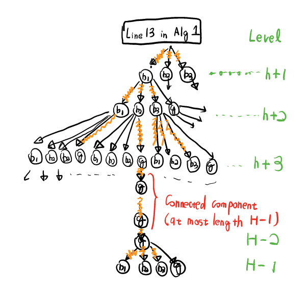
Then, the total sample complexity is upper-bounded by

$\displaystyle\underbrace{HMI_{\max}}_{(a)}+\underbrace{\sum_{m=1}^{I_{\max}}(M+M^{\prime}(A+1))H\alpha_{m}+(M/A+M^{\prime}(A+1))H\beta_{m}\}}_{(b)}.$

The term (a) comes from samples we use lineย 4 to lineย 7 in Algorithmย 1. Note $H$ is the number of samples we need to reset, $M$ is the number of samples in $\hat{x}_{h}(a_{0:h-1})$ and $N^{\prime}$ upper-bounds the number of iterations in the main loop. Next, we see the term (b). Here, $M^{\prime}$ is the number of samples in $\hat{r}_{h}$. More specifically, we need $MH$ samples in lineย 6 in Algorithmย 2, which we traverse in both good and bad events (per bad event, we just use $MH/A$ samples). Additionally, we need $M^{\prime}H$ samples in lineย 10 in Algorithmย 2 in good events and $M^{\prime}H$ samples in lineย 14 in Algorithmย 2 in bad events. When we call $H-1$, we use additionally use $AM^{\prime}H$ samples. For each visit, we use at most $(A+1)M^{\prime}H$ samples in lineย 3.

Next, we show $\alpha_{m}\leq H\beta_{m}$. First, we denote sets of all $g$ and $b_{a}$ nodes the algorithm traverse at iteration $m$ in the tree by $G_{m}$ and $B_{m}$, respectively. We denote a subgraph on the tree consisting of nodes and edges which the algorithm traverses by $\tilde{\Omega}_{m}$. We denote a subgraph in $\tilde{\Omega}_{m}$ consisting of nodes $G_{m}$ and edges whose both sides belong to $G_{m}$ by $\tilde{G}_{m}$. We divide $\tilde{G}_{m}$ into connected components on $\tilde{\Omega}_{m}$. Here, each component has at most $H$ nodes. The most upstream node in a component is adjacent to some node in $B_{m}$ on $\tilde{\Omega}_{m}$. Besides, this node in $B_{m}$ is not shared by other connected components in $\tilde{G}_{m}$. This ensures that $\alpha_{m}\leq H\beta_{m}$.

Finally, we use $\sum_{m}\beta_{m}\leq O(HAd/\varepsilon^{2}\ln(1/\varepsilon))$ as we see the number of times we call Line 11 in Algorithm 1 and Line 11 in Algorithm 2 at $h\in[H]$ is upper-bounded by $O(d/\varepsilon^{2}\ln(1/\varepsilon))$ and we multiply it by $HA$. Thus,

$\displaystyle HMI_{\max}+\sum_{m=1}^{I_{\max}}(M+M^{\prime}(A+1))H\alpha_{m}+(M/A+M^{\prime}(A+1))H\beta_{m}\}$
$\displaystyle=O((M+M^{\prime})H^{3}A^{2}d/\varepsilon^{2}\ln(1/\varepsilon)).$

โˆŽ

In this lemma, as a corollary, the following statement holds:

  • โ€ข

    The number of times we visit lineย 6 in Algorithmย 2 is upper-bounded by $\sum_{m}(\beta_{m}/A+\alpha_{m})$.

  • โ€ข

    The number of times we visit lineย 3, lineย 9 and lineย 13 in Algorithmย 2 is upper-bounded by $\sum_{m}(\beta_{m}+\alpha_{m})(A+1)$.

Here, we have

$\displaystyle\sum_{m=1}^{I_{\max}}\beta_{m}=O(HAd/\varepsilon^{2}\ln(1/\varepsilon)),\quad\sum_{m=1}^{I_{\max}}\alpha_{m}=O(H^{2}Ad/\varepsilon^{2}\ln(1/\varepsilon)).$

C.2 Second Step

We prove some lemma which implies that Algorithmย 2 always returns a good estimate of Vhโ‹†โ€‹(shโ€‹(a0:hโˆ’1))subscriptsuperscript๐‘‰โ‹†โ„Žsubscript๐‘ โ„Žsubscript๐‘Ž:0โ„Ž1V^{\star}_{h}(s_{h}(a_{0:h-1})) in the algorithm in high probability. Before providing the statement, we explain several events we need to condition on.

C.2.1 Preparation

We first note for in the data $\mathcal{D}_{a;h}$, a value $y_{a:h}$ corresponding to $\hat{x}_{h}(a_{0:h-1})$ is always in the form of

ya:h=๐”ผโ€‹[โˆ‘k=hHrkโˆฃshโ€‹(a1:hโˆ’1);ah=a,ah+1:Hโˆ’1=ah+1:Hโˆ’1โ€ฒ]+โˆ‘k=hHฮฝk,ฮฝk=1/Mโ€ฒโ€‹โˆ‘i=1Mโ€ฒฯ„k[i]formulae-sequencesubscript๐‘ฆ:๐‘Žโ„Ž๐”ผdelimited-[]formulae-sequenceconditionalsuperscriptsubscript๐‘˜โ„Ž๐ปsubscript๐‘Ÿ๐‘˜subscript๐‘ โ„Žsubscript๐‘Ž:1โ„Ž1subscript๐‘Žโ„Ž๐‘Žsubscript๐‘Ž:โ„Ž1๐ป1subscriptsuperscript๐‘Žโ€ฒ:โ„Ž1๐ป1superscriptsubscript๐‘˜โ„Ž๐ปsubscript๐œˆ๐‘˜subscript๐œˆ๐‘˜1superscript๐‘€โ€ฒsuperscriptsubscript๐‘–1superscript๐‘€โ€ฒsubscriptsuperscript๐œdelimited-[]๐‘–๐‘˜\displaystyle y_{a:h}=\mathbb{E}[\sum_{k=h}^{H}r_{k}\mid s_{h}(a_{1:h-1});a_{h}=a,a_{h+1:H-1}=a^{\prime}_{h+1:H-1}]+\sum_{k=h}^{H}\nu_{k},\quad\nu_{k}=1/M^{\prime}\sum_{i=1}^{M^{\prime}}\tau^{[i]}_{k}

for some (random) action sequence $a^{\prime}_{h:H-1}$. Note this is not a high probability statement. Here, $\tau_{a;h}$ is an i.i.d noise in rewards which come from lineย 3 in Algorithmย 2 (when $h=H-1$), lineย 9 in Algorithmย 2 (good events in when $h<H-1$), and in lineย 13 in Algorithmย 2 (bad events in when $h<H-1$). We denote the whole noise part in $y_{a:h}$ by

$\displaystyle z_{a;h}=\sum_{k=h}^{H}\nu_{k}.$

C.2.2 Events we need to condition on

In the lemma, we need to condition on two types of events.

First event

Firstly, we condition on the event

$\displaystyle\forall a\in\mathcal{A};|\langle\theta^{\star}_{a;h},x_{h}(a_{0:h-1})-\hat{x}_{h}(a_{0:h-1})\rangle|\leq\min\left(\frac{\Delta}{6},\frac{\Delta}{12\sqrt{N^{\prime}\varepsilon}}\right)$ (5)

every time we visit lineย 6 in Algorithmย 2 and lineย 5 in Algorithmย 1. The concentration is obtained noting $\theta_{a;h}^{\top}\{\hat{x}_{h}(a_{0:h-1})-x_{h}(a_{0:h-1})\}$ is a $\Theta^{2}/M$ sub-Gaussian random variable with mean zero conditional on $x_{h}(a_{0:h-1})$. Formally, by properly setting $M$, we use the following lemma (simple application of Hoeffedingโ€™s inequality).

Lemma 5 (Concentration of feature estimators).

With probability $1-\delta^{\prime}$,

$\displaystyle\forall a;|\langle\theta^{\star}_{a;h},x_{h}(a_{0:h-1})-\hat{x}_{h}(a_{0:h-1})\rangle|\leq\Theta\sqrt{\ln(A/\delta^{\prime})/M}.$

We later choose $M$ so that (5) holds. Note the number of visitation is

$$I_{\max}H+\sum_{m}(\alpha_{m}+\beta_{m}/A)=O(H^{2}Ad/\varepsilon^{2}\ln(1/\varepsilon)).$$

We take the union bound later.

Second event

We condition on the event

$\displaystyle|\nu_{k}|\leq\min\left\{\Delta/(6H),\frac{\Delta}{12\sqrt{N^{\prime}\varepsilon}}\right\}$ (6)

every time we visit lineย 3 in Algorithmย 2 (when $h=H-1$), lineย 13 in Algorithmย 2 (good events in $h\leq H-1$), and lineย 15 in Algorithmย 2 (bad events in $h\leq H-1$). By properly setting $M^{\prime}$, the concentration is obtained noting $\nu_{k}$ is a $1/M^{2}$-sub-Gaussian variable as follows. This is derived as a simple application of Hoeffedingโ€™s inequality.

Lemma 6 (Concentration of reward estimators).

With probability $1-\delta^{\prime}$,

$\displaystyle|\nu_{k}|\leq 2\sqrt{\ln(1/\delta^{\prime})/M^{\prime}}.$

Later, we choose $M^{\prime}$ so that (6) is satisfied. Note the number of times we visit is

$$\sum_{m=1}^{I_{\max}}(\alpha_{m}+\beta_{m})(A+1)=O((M+M^{\prime})H^{2}A^{2}d/\epsilon^{2}\ln(1/\epsilon)).$$

We take the union bound later.

Accuracy of $\text{Compute-}V^{\star}$

When the above events hold, we can ensure Algorithmย 2 always returns Vhโ‹†โ€‹(shโ€‹(a0:hโˆ’1))subscriptsuperscript๐‘‰โ‹†โ„Žsubscript๐‘ โ„Žsubscript๐‘Ž:0โ„Ž1V^{\star}_{h}(s_{h}(a_{0:h-1})) with some small deviation error.

Lemma 7 (The accuracy of $\text{Compute-}V^{\star}$).

We set $\varepsilon$ such that $\varepsilon=\Delta/(6\Theta)$. Let $a^{\star}_{h:H}(a_{0:h-1})\in\mathcal{A}^{H-h}$ be the optimal action sequence from $h$ to $H-1$ after $a_{0:h-1}$. We condition on the events we have mentioned above. Then, in the algorithm, we always have

Compute-โ€‹Vโ‹†โ€‹(h;a0:hโˆ’1)=Vhโ‹†โ€‹(shโ€‹(a0:hโˆ’1))+โˆ‘k=hHโˆ’1ฮฝk.Compute-superscript๐‘‰โ‹†โ„Žsubscript๐‘Ž:0โ„Ž1subscriptsuperscript๐‘‰โ‹†โ„Žsubscript๐‘ โ„Žsubscript๐‘Ž:0โ„Ž1superscriptsubscript๐‘˜โ„Ž๐ป1subscript๐œˆ๐‘˜\text{Compute-}V^{\star}(h;a_{0:h-1})=V^{\star}_{h}(s_{h}(a_{0:h-1}))+\sum_{k=h}^{H-1}\nu_{k}.
Proof.

We prove by induction. We want to prove this statement for any query we have in the algorithm. Suppose we already visit Line 11 in Algorithm 1 $m-1$ times. In other words, we are now at the episode at $m$. Thus, we use induction in the sense that assuming the statement holds in all queries in the previous episodes before $m$ and all queries from level $h+1$ to level $H-1$ in episode $m$, we want to prove the statement holds for all queries at level $h$ in episode $m$.

We first start with the base case level $H-1$ at episode $m$. When $h=H-1$, our procedure simply returns maxaโกr^Hโˆ’1โ€‹(sHโˆ’1โ€‹(a0:Hโˆ’2),a)subscript๐‘Žsubscript^๐‘Ÿ๐ป1subscript๐‘ ๐ป1subscript๐‘Ž:0๐ป2๐‘Ž\max_{a}\hat{r}_{H-1}(s_{H-1}(a_{0:H-2}),a). From the gap assumption, we have maxaโกr^Hโˆ’1โ€‹(sHโˆ’1โ€‹(a0:Hโˆ’2),a)=maxaโˆˆ๐’œโกrHโˆ’1โ€‹(sHโˆ’1โ€‹(a0:Hโˆ’2),a)subscript๐‘Žsubscript^๐‘Ÿ๐ป1subscript๐‘ ๐ป1subscript๐‘Ž:0๐ป2๐‘Žsubscript๐‘Ž๐’œsubscript๐‘Ÿ๐ป1subscript๐‘ ๐ป1subscript๐‘Ž:0๐ป2๐‘Ž\max_{a}\hat{r}_{H-1}(s_{H-1}(a_{0:H-2}),a)=\max_{a\in\mathcal{A}}r_{H-1}(s_{H-1}(a_{0:H-2}),a) noting we condition on the event the difference is upper-bounded by $\Delta/(6H)$ from (6). Thus, VHโˆ’1โ‹†โ€‹(sHโˆ’1โ€‹(a0:Hโˆ’2))+ฮฝHโˆ’1subscriptsuperscript๐‘‰โ‹†๐ป1subscript๐‘ ๐ป1subscript๐‘Ž:0๐ป2subscript๐œˆ๐ป1V^{\star}_{H-1}(s_{H-1}(a_{0:H-2}))+\nu_{H-1} by definition.

Now assume that the conclusion holds for all queries at level $h+1$ in episode $m$ and all queries in the previous episodes before episode $m$. We prove the statement also holds for all queries at level $h$ in episode $m$ when $h<H-1$.

We divide into two cases.

Case 1: $\|\hat{x}_{h}(a_{0:h-1})\|_{\Sigma^{-1}_{h}}>\varepsilon$

The first case is $\|\hat{x}_{h}(a_{0:h-1})\|_{\Sigma^{-1}_{h}}>\varepsilon$. In this case, we aim to calculate Qhโ‹†โ€‹(shโ€‹(a0:hโˆ’1),aโ€ฒ)subscriptsuperscript๐‘„โ‹†โ„Žsubscript๐‘ โ„Žsubscript๐‘Ž:0โ„Ž1superscript๐‘Žโ€ฒQ^{\star}_{h}(s_{h}(a_{0:h-1}),a^{\prime}) for all $a^{\prime}\in\mathcal{A}$ by calling $\text{Compute-}V^{\star}$ at layer $h+1$ with input $\{a_{0:h-1},a^{\prime}\}$. Note that by inductive hypothesis, we have

Compute-โ€‹Vโ‹†โ€‹(h+1;{a0:hโˆ’1,aโ€ฒ})=Vh+1โ‹†โ€‹(shโ€‹(a0:hโˆ’1,aโ€ฒ))+โˆ‘k=h+1Hโˆ’1ฮฝk.Compute-superscript๐‘‰โ‹†โ„Ž1subscript๐‘Ž:0โ„Ž1superscript๐‘Žโ€ฒsubscriptsuperscript๐‘‰โ‹†โ„Ž1subscript๐‘ โ„Žsubscript๐‘Ž:0โ„Ž1superscript๐‘Žโ€ฒsuperscriptsubscript๐‘˜โ„Ž1๐ป1subscript๐œˆ๐‘˜\displaystyle\text{Compute-}V^{\star}(h+1;\{a_{0:h-1},a^{\prime}\})=V^{\star}_{h+1}(s_{h}(a_{0:h-1},a^{\prime}))+\sum_{k=h+1}^{H-1}\nu_{k}.

Hence, from the definition of $y_{a^{\prime};h}$,

$\displaystyle y_{a^{\prime};h}$ $\displaystyle=\hat{r}_{h}(s_{h}(a_{0:h-1},a^{\prime})+V^{\star}_{h+1}(s_{h}(a_{0:h-1},a^{\prime}))+\sum_{k=h+1}^{H-1}\nu_{k}$
=Qhโ‹†โ€‹(shโ€‹(a0:hโˆ’1),aโ€ฒ)+โˆ‘k=hHโˆ’1ฮฝk.absentsubscriptsuperscript๐‘„โ‹†โ„Žsubscript๐‘ โ„Žsubscript๐‘Ž:0โ„Ž1superscript๐‘Žโ€ฒsuperscriptsubscript๐‘˜โ„Ž๐ป1subscript๐œˆ๐‘˜\displaystyle=Q^{\star}_{h}(s_{h}(a_{0:h-1}),a^{\prime})+\sum_{k=h}^{H-1}\nu_{k}.

Thus, noting we condition on the event $\nu_{k}$ are upper-bounded by $\Delta/(6H)$ in the algorithm, we have

|yaโ€ฒ;hโˆ’Qhโ‹†โ€‹(shโ€‹(a0:hโˆ’1),aโ€ฒ)|โ‰ค(Hโˆ’h)โ€‹ฮ”/(6โ€‹H).subscript๐‘ฆsuperscript๐‘Žโ€ฒโ„Žsubscriptsuperscript๐‘„โ‹†โ„Žsubscript๐‘ โ„Žsubscript๐‘Ž:0โ„Ž1superscript๐‘Žโ€ฒ๐ปโ„Žฮ”6๐ป|y_{a^{\prime};h}-Q^{\star}_{h}(s_{h}(a_{0:h-1}),a^{\prime})|\leq(H-h)\Delta/(6H).

From the gap assumption (Assumption 4), thus argmaxaโ€ฒyaโ€ฒ;h=argmaxaโ€ฒQhโ‹†โ€‹(shโ€‹(a0:hโˆ’1),aโ€ฒ)=ahโ‹†โ€‹(a0:hโˆ’1)subscriptargmaxsuperscript๐‘Žโ€ฒsubscript๐‘ฆsuperscript๐‘Žโ€ฒโ„Žsubscriptargmaxsuperscript๐‘Žโ€ฒsubscriptsuperscript๐‘„โ‹†โ„Žsubscript๐‘ โ„Žsubscript๐‘Ž:0โ„Ž1superscript๐‘Žโ€ฒsubscriptsuperscript๐‘Žโ‹†โ„Žsubscript๐‘Ž:0โ„Ž1\mathop{\mathrm{argmax}}_{a^{\prime}}y_{a^{\prime};h}=\mathop{\mathrm{argmax}}_{a^{\prime}}Q^{\star}_{h}(s_{h}(a_{0:h-1}),a^{\prime})=a^{\star}_{h}(a_{0:h-1}). Thus, after choosing the optimal action we return

Vhโ‹†โ€‹(shโ€‹(a0:hโˆ’1))+โˆ‘k=hHโˆ’1ฮฝk.subscriptsuperscript๐‘‰โ‹†โ„Žsubscript๐‘ โ„Žsubscript๐‘Ž:0โ„Ž1superscriptsubscript๐‘˜โ„Ž๐ป1subscript๐œˆ๐‘˜\displaystyle V^{\star}_{h}(s_{h}(a_{0:h-1}))+\sum_{k=h}^{H-1}\nu_{k}.

This implies that the conclusion holds for queries at level $h$ in the first case.

Case 2: $\|\hat{x}_{h}(a_{0:h-1})\|_{\Sigma^{-1}_{h}}\leq\varepsilon$

The second case is $\|\hat{x}_{h}(a_{0:h-1})\|_{\Sigma^{-1}_{h}}\leq\varepsilon$. We first note from the inductive hypothesis, in the data $\mathcal{D}_{a;h}$, for any $\hat{x}_{h}(a_{0:h-1})$, the corresponding $y_{a;h}$ is

$\displaystyle y_{a;h}$ =Qhโ‹†โ€‹(shโ€‹(a0:hโˆ’1),a)+โˆ‘k=hHฮฝkabsentsubscriptsuperscript๐‘„โ‹†โ„Žsubscript๐‘ โ„Žsubscript๐‘Ž:0โ„Ž1๐‘Žsuperscriptsubscript๐‘˜โ„Ž๐ปsubscript๐œˆ๐‘˜\displaystyle=Q^{\star}_{h}(s_{h}(a_{0:h-1}),a)+\sum_{k=h}^{H}\nu_{k}

Recall that Qhโ‹†โ€‹(shโ€‹(a0:hโˆ’1),a)=(ฮธa;hโ‹†)โŠคโ€‹xhโ€‹(a0:hโˆ’1)subscriptsuperscript๐‘„โ‹†โ„Žsubscript๐‘ โ„Žsubscript๐‘Ž:0โ„Ž1๐‘Žsuperscriptsuperscriptsubscript๐œƒ๐‘Žโ„Žโ‹†topsubscript๐‘ฅโ„Žsubscript๐‘Ž:0โ„Ž1Q^{\star}_{h}(s_{h}(a_{0:h-1}),a)=(\theta_{a;h}^{\star})^{\top}x_{h}(a_{0:h-1}). Then, for any $a\in\mathcal{A}$,

$\displaystyle\hat{\theta}_{a;h}$ $\displaystyle=\Sigma^{-1}_{h}\sum_{i=1}^{|\mathcal{D}_{a;h}|}\hat{x}^{(i)}_{h}(a_{0:h-1})\{\langle x^{(i)}_{h}(a_{0:h-1}),\theta^{\star}_{a;h}\rangle+z^{(i)}_{a;h}\}$
$\displaystyle=\Sigma^{-1}_{h}\sum_{i=1}^{|\mathcal{D}_{a;h}|}\hat{x}_{h}(a_{0:h-1})\{\langle x^{(i)}_{h}(a_{0:h-1})-\hat{x}^{(i)}_{h}(a_{0:h-1}),\theta^{\star}_{a;h}\rangle+\langle\hat{x}^{(i)}_{h}(a_{0:h-1}),\theta^{\star}_{a;h}\rangle+z^{(i)}_{a;h}\}$
$\displaystyle=\theta^{\star}_{a;h}-\lambda\Sigma^{-1}_{h}\theta^{\star}_{a;h}+\Sigma^{-1}_{h}\sum_{i=1}^{|\mathcal{D}_{a;h}|}\hat{x}^{(i)}_{h}(a_{0:h-1})\{\langle x^{(i)}_{h}(a_{0:h-1})-\hat{x}^{(i)}_{h}(a_{0:h-1}),\theta^{\star}_{a;h}\rangle+z^{(i)}_{a;h}\}$
$\displaystyle=\theta^{\star}_{a;h}-\lambda\Sigma^{-1}_{h}\theta^{\star}_{a;h}+\Sigma^{-1}_{h}\sum_{i=1}^{|\mathcal{D}_{a;h}|}\hat{x}^{(i)}_{h}(a_{0:h-1})w^{(i)}_{a;h}$

where $w^{(i)}_{a;h}=\langle\hat{x}^{(i)}_{h}(a_{0:h-1})-x^{(i)}_{h}(a_{0:h-1}),\theta^{\star}_{a;h}\rangle+z^{(i)}_{a;h}$. On the events we condition ((5) and (6)), we have $|w^{(i)}_{a;h}|\leq\mathrm{Error}$ where

$\displaystyle\mathrm{Error}:=\Delta/(6\sqrt{N^{\prime}\varepsilon}).$

Using the above, at level $h$ in episode $m$,

$\displaystyle\forall a:\left\lvert\hat{\theta}_{a;h}^{\top}\hat{x}_{h}(a_{0:h-1})-(\theta_{a;h}^{\star})^{\top}{x}_{h}(a_{0:h-1})\right\rvert$
$\displaystyle\leq\left\lvert(\hat{\theta}_{a;h}-\theta^{\star}_{a;h})^{\top}\hat{x}_{h}(a_{0:h-1})\right\rvert+\left\lvert(\theta^{\star}_{a;h})^{\top}(\hat{x}_{h}(a_{0:h-1})-x_{h}(a_{0:h-1}))\right\rvert$
$\displaystyle\leq\underbrace{\left\lvert\langle\lambda\Sigma^{-1}_{h}\theta^{\star}_{a;h},\hat{x}_{h}(a_{0:h-1})\rangle\right\rvert}_{(a)}+\underbrace{\left\lvert\langle\Sigma^{-1}_{h}\sum_{i=1}^{|\mathcal{D}_{a;h}|}\hat{x}^{(i)}_{h}(a_{0:h-1})w^{(i)}_{a;h},\hat{x}_{h}(a_{0:h-1})\rangle\right\lvert}_{(b)}+\Delta/6.$ (Use (5) )

The first term (a) is upper-bounded by

$\displaystyle\left\lvert\langle\lambda\Sigma^{-1}_{h}\theta^{\star}_{a;h},\hat{x}_{h}(a_{0:h-1})\rangle\right\rvert$ $\displaystyle\leq\lambda\|\Sigma^{-1}_{h}\theta^{\star}_{a;h}\|_{\Sigma_{h}}\|\hat{x}_{h}(a_{0:h-1})\|_{\Sigma^{-1}_{h}}$ (CS inequality)
$\displaystyle\leq\sqrt{\lambda}\Theta\varepsilon$ ($\theta^{\star}_{a;h}\leq\Theta$ and $\|\hat{x}_{h}(a_{0:h-1})\|_{\Sigma^{-1}_{h}}\leq\varepsilon$)
$\displaystyle\leq\Delta/6.$ (We set a parameter $\varepsilon$ to satisfy this condition)

The second term (b) is upper-bounded by

$\displaystyle\mathrm{Error}\times\sum_{i=1}^{|\mathcal{D}_{a;h}|}|\hat{x}^{\top}_{h}(a_{0:h-1})\Sigma^{-1}_{h}x^{(i)}_{h}(a_{0:h-1})|$
$\displaystyle\leq\mathrm{Error}\times\sqrt{|\mathcal{D}_{a;h}|\hat{x}^{\top}_{h}\Sigma^{-1}_{h}\sum_{i=1}^{|\mathcal{D}_{a;h}|}x^{(i)}_{h}(a_{0:h-1})x^{(i)}_{h}(a_{0:h-1})^{\top}\Sigma^{-1}_{h}\hat{x}_{h}}$ (From L1 norm to L2 norm)
$\displaystyle\leq\mathrm{Error}\times\sqrt{N^{\prime}\hat{x}^{\top}_{h}\Sigma^{-1}_{h}\sum_{i=1}^{|\mathcal{D}_{a;h}|}x^{(i)}_{h}(a_{0:h-1})x^{(i)}_{h}(a_{0:h-1})^{\top}\Sigma^{-1}_{h}\hat{x}_{h}}$ ($N^{\prime}$ upper-bounds $|\mathcal{D}_{a;h}|$)
$\displaystyle\leq\mathrm{Error}\times\sqrt{N^{\prime}\varepsilon}$
$\displaystyle\leq\Delta/6.$ (We set $M,M^{\prime},\varepsilon$ to satisfy this condition )

From the third line to the fourth line, we use a general fact when $x^{\top}(C+\lambda I)^{-1}x\leq\varepsilon$ is satisfied, we have $x^{\top}(C+\lambda I)^{-1}C(C+\lambda I)^{-1}x\leq\varepsilon$ for any matrix $C$ and vector $x$.

Thus, we have that:

$\displaystyle\forall a:\left\lvert\hat{\theta}_{a;h}^{\top}\hat{x}_{h}(a_{0:h-1})-(\theta_{a;h}^{\star})^{\top}{x}_{h}(a_{0:h-1})\right\rvert\leq\Delta/2.$

Together with the gap assumption, this means

$$\mathop{\mathrm{argmax}}_{a}\hat{\theta}_{a;h}^{\top}\hat{x}_{h}(a_{0:h-1})=\mathop{\mathrm{argmax}}_{a}(\theta^{\star}_{a;h})^{\top}x_{h}(a_{0:h-1})=a^{\star}_{h}(a_{0:h-1}).$$

Thus, we select $a^{\star}_{h}(a_{0:h-1})$ at $h$. Then, when we query $\text{Compute-}V^{\star}(h+1;\{a_{0:h-1},a^{\star}_{h}(a_{0:h-1})\})$, which by inductive hypothesis we return

Vh+1โ‹†โ€‹(sh+1โ€‹({a0:hโˆ’1,ahโ‹†โ€‹(a0:hโˆ’1)}))+โˆ‘k=h+1Hโˆ’1ฮฝk.subscriptsuperscript๐‘‰โ‹†โ„Ž1subscript๐‘ โ„Ž1subscript๐‘Ž:0โ„Ž1subscriptsuperscript๐‘Žโ‹†โ„Žsubscript๐‘Ž:0โ„Ž1superscriptsubscript๐‘˜โ„Ž1๐ป1subscript๐œˆ๐‘˜\displaystyle V^{\star}_{h+1}(s_{h+1}(\{a_{0:h-1},a^{\star}_{h}(a_{0:h-1})\}))+\sum_{k=h+1}^{H-1}\nu_{k}.

Finally, adding the reward, we return

Vhโ‹†โ€‹(shโ€‹(a0:hโˆ’1))+โˆ‘k=hHโˆ’1ฮฝk.subscriptsuperscript๐‘‰โ‹†โ„Žsubscript๐‘ โ„Žsubscript๐‘Ž:0โ„Ž1superscriptsubscript๐‘˜โ„Ž๐ป1subscript๐œˆ๐‘˜\displaystyle V^{\star}_{h}(s_{h}(a_{0:h-1}))+\sum_{k=h}^{H-1}\nu_{k}.

This implies that the conclusion holds for any queries at level h in the second case. โˆŽ

C.3 Third Step

The next lemma shows that when the algorithm terminates, we must find an exact optimal policy.

Lemma 8 (Optimality upon termination).

Algorithmย 1 returns an optimal policy on termination.

Proof.

Recall we denote the optimal trajectory by {shโ‹†,ahโ‹†}h=0Hโˆ’1superscriptsubscriptsuperscriptsubscript๐‘ โ„Žโ‹†superscriptsubscript๐‘Žโ„Žโ‹†โ„Ž0๐ป1\{s_{h}^{\star},a_{h}^{\star}\}_{h=0}^{H-1} where shโ‹†=shโ€‹(a0:hโˆ’1โ‹†)subscriptsuperscript๐‘ โ‹†โ„Žsubscript๐‘ โ„Žsubscriptsuperscript๐‘Žโ‹†:0โ„Ž1s^{\star}_{h}=s_{h}(a^{\star}_{0:h-1}). Upon termination of Algorithmย 1, we have $\forall h:\|\hat{x}_{h}(a_{0:h-1})\|_{\Sigma_{h}^{-1}}\leq\varepsilon$. We prove the theorem by induction. At $h=0$, we know that s0=s0โ‹†subscript๐‘ 0superscriptsubscript๐‘ 0โ‹†s_{0}=s_{0}^{\star}. By our linear regression guarantee as we see in the second step of the proof, we can ensure that for all $a\in\mathcal{A}$,

$\displaystyle\left\lvert\theta_{a;0}^{\top}\hat{x}_{0}-(\theta^{\star}_{a;0})^{\top}x_{0}\right\rvert\leq\Delta/2,$

which means that $a_{0}=\mathop{\mathrm{argmax}}_{a}\theta_{a;0}^{\top}x_{0}=a_{0}^{\star}$. This completes the base case.

Now we assume it holds a step 00 to $h$. We prove the statement for step $h+1$. Thus, we can again use the linear regression guarantee to show that the prediction error for all $a$ must be less than $\Delta/2$, i.e.,

$\displaystyle\left\lvert\theta_{a;h}^{\top}\hat{x}_{h}(a^{\star}_{0:h-1})-(\theta^{\star}_{a;h})^{\top}x_{h}(a^{\star}_{0:h-1})\right\rvert\leq\Delta/2.$

This indicates that at $h+1$, we will pick the correct action $a_{h+1}^{\star}$. This completes the proof. โˆŽ

Finally, combining lemmas so far, we derive the final sample complexity.

Theorem 8.

With probability $1-\delta$, the algorithms output the optimal actions after using at most the following number of samples

$\displaystyle\tilde{O}\left(\frac{H^{5}A\Theta^{5}d^{2}\ln(1/\delta)}{\Delta^{5}}\right).$

Here, we ignore $\mathrm{Polylog}(H,d,\ln(1/\delta),1/\Delta,|\mathcal{A}|,\Theta)$.

Proof.

Recall we use the following number of samples:

$\displaystyle O((M+M^{\prime})H^{3}Ad/\varepsilon^{2}\ln(d/\varepsilon))$

Here, the rest of the task is to properly set $M,M^{\prime},\varepsilon$.

Number of times we use concentration inequalities

We use high probability statements to bound three-types of terms:

$\displaystyle\forall a\in\mathcal{A};|\langle\theta^{\star}_{a;h},\hat{x}_{h}(a_{0:h-1})-x_{h}(a_{0:h-1})\rangle|\leq 2\Theta\sqrt{\ln(1/\delta^{\prime})/M},$ (7)
$\displaystyle|\nu_{k}|\leq 2\sqrt{\ln(1/\delta^{\prime})/M^{\prime}}.$ (8)

Let $N^{\prime}=O(Hd/\varepsilon^{2}\ln(d/\varepsilon))$. We also set $\varepsilon=O(\Delta/\Theta)$. Recall we need to set $M$ and $M^{\prime}$ such that

$\displaystyle 2\Theta\sqrt{\ln(1/\delta^{\prime})/M}$ $\displaystyle\leq\min\left(\Delta/6,\Delta/(12\sqrt{N^{\prime}\varepsilon})\right),\quad 2\sqrt{\ln(1/\delta^{\prime})/M^{\prime}}\leq\min\left(\Delta/(6H),\Delta/(12\sqrt{N^{\prime}\varepsilon})\right).$

Thus, we set

$\displaystyle M=O\left(\frac{\ln(1/\delta^{\prime})\Theta^{3}Hd\ln(d\Theta/\Delta)}{\Delta^{3}}\right),\quad M^{\prime}=O\left(\frac{\ln(1/\delta^{\prime})\Theta H^{2}d\ln(d\Theta/\Delta)}{\Delta^{3}}\right).$

Here, events (7) and (8) are called $O(\sum(\alpha_{m}+\beta_{m}))$ times. Thus, we set $\delta^{\prime}=\delta/(\sum(\alpha_{m}+\beta_{m})$.

Collect all events

Recall we need the following number of samples:

$\displaystyle O\left((M+M^{\prime})H^{3}A^{2}d/\varepsilon^{2}\ln(d/\varepsilon)\right).$

Thus, the total sample complexity is

$\displaystyle N=\tilde{O}\left(\frac{H^{2}d\Theta^{3}\ln(1/\delta^{\prime})}{\Delta^{3}}\times\frac{H^{3}A^{2}d\times\Theta^{2}}{\Delta^{2}}\right)$

where $1/\delta^{\prime}=1/\delta\times O(\sum(\alpha_{m}+\beta_{m})$. Hence,

$\displaystyle N=\tilde{O}\left(\frac{H^{5}A^{2}\Theta^{5}d^{2}\ln(1/\delta)}{\Delta^{5}}\right).$

โˆŽ

Appendix D Proof of Sectionย B

D.1 Proof of Lemmaย 3

Since aโŠคโ€‹ฯ•โ€‹(s)โˆˆโ„‹๐’ฎยฏsuperscript๐‘Žtopitalic-ฯ•๐‘ subscriptโ„‹ยฏ๐’ฎa^{\top}\phi(s)\in\mathcal{H}_{\bar{\mathcal{S}}}, it can be written in the form of

aโŠคโ€‹ฯ•โ€‹(โ‹…)=โˆ‘i=1โˆžฮฑiโ€‹kยฏโ€‹(โ‹…,s[i]).superscript๐‘Žtopitalic-ฯ•โ‹…superscriptsubscript๐‘–1subscript๐›ผ๐‘–ยฏ๐‘˜โ‹…superscript๐‘ delimited-[]๐‘–\displaystyle a^{\top}\phi(\cdot)=\sum_{i=1}^{\infty}\alpha_{i}\bar{k}(\cdot,s^{[i]}).

where s[i]โˆˆ๐’ฎsuperscript๐‘ delimited-[]๐‘–๐’ฎs^{[i]}\in{\mathcal{S}}. Then, it is equal to

โˆ‘i=1โˆžฮฑiโ€‹kยฏโ€‹(โ‹…,s(i))=โˆ‘i=1โˆžฮฑiโ€‹๐”ผoโ€ฒโˆผ๐•†โ€‹(s(i)),oโˆผ๐•†โ€‹(โ‹…)โ€‹[ฯˆโŠคโ€‹(oโ€ฒ)โ€‹ฯˆโ€‹(o)]superscriptsubscript๐‘–1subscript๐›ผ๐‘–ยฏ๐‘˜โ‹…superscript๐‘ ๐‘–superscriptsubscript๐‘–1subscript๐›ผ๐‘–subscript๐”ผformulae-sequencesimilar-tosuperscript๐‘œโ€ฒ๐•†superscript๐‘ ๐‘–similar-to๐‘œ๐•†โ‹…delimited-[]superscript๐œ“topsuperscript๐‘œโ€ฒ๐œ“๐‘œ\displaystyle\sum_{i=1}^{\infty}\alpha_{i}\bar{k}(\cdot,s^{(i)})=\sum_{i=1}^{\infty}\alpha_{i}\mathbb{E}_{o^{\prime}\sim\mathbb{O}(s^{(i)}),o\sim\mathbb{O}(\cdot)}[\psi^{\top}(o^{\prime})\psi(o)]
=โŸจโˆ‘i=1โˆžฮฑiโ€‹๐”ผoโ€ฒโˆผ๐•†โ€‹(s(i))โ€‹[ฯˆโŠคโ€‹(oโ€ฒ)],๐”ผoโˆผ๐•†โ€‹(โ‹…)โ€‹[ฯˆโ€‹(o)]โŸฉabsentsuperscriptsubscript๐‘–1subscript๐›ผ๐‘–subscript๐”ผsimilar-tosuperscript๐‘œโ€ฒ๐•†superscript๐‘ ๐‘–delimited-[]superscript๐œ“topsuperscript๐‘œโ€ฒsubscript๐”ผsimilar-to๐‘œ๐•†โ‹…delimited-[]๐œ“๐‘œ\displaystyle=\langle\sum_{i=1}^{\infty}\alpha_{i}\mathbb{E}_{o^{\prime}\sim\mathbb{O}(s^{(i)})}[\psi^{\top}(o^{\prime})],\mathbb{E}_{o\sim\mathbb{O}(\cdot)}[\psi(o)]\rangle

Thus, there exists $b$ s.t. $a^{\top}\phi(\cdot)=b^{\top}\mathbb{E}_{o\sim\mathbb{O}(\cdot)}[\psi(o)]$. Finally,

1โ‰ฅaโŠคโ€‹๐”ผsโˆผuSโ€‹(s)โ€‹[ฯ•โ€‹(s)โ€‹ฯ•โŠคโ€‹(s)]โ€‹a=bโŠคโ€‹๐”ผsโˆผuSโ€‹(s)โ€‹[๐”ผoโˆผ๐•†โ€‹(s)โ€‹[ฯˆโ€‹(o)]โ€‹๐”ผoโˆผ๐•†โ€‹(s)โ€‹[ฯˆโŠคโ€‹(oโ€ฒ)]]โ€‹b1superscript๐‘Žtopsubscript๐”ผsimilar-to๐‘ subscript๐‘ข๐‘†๐‘ delimited-[]italic-ฯ•๐‘ superscriptitalic-ฯ•top๐‘ ๐‘Žsuperscript๐‘topsubscript๐”ผsimilar-to๐‘ subscript๐‘ข๐‘†๐‘ delimited-[]subscript๐”ผsimilar-to๐‘œ๐•†๐‘ delimited-[]๐œ“๐‘œsubscript๐”ผsimilar-to๐‘œ๐•†๐‘ delimited-[]superscript๐œ“topsuperscript๐‘œโ€ฒ๐‘\displaystyle 1\geq a^{\top}\mathbb{E}_{s\sim u_{S}(s)}[\phi(s)\phi^{\top}(s)]a=b^{\top}\mathbb{E}_{s\sim u_{S}(s)}[\mathbb{E}_{o\sim\mathbb{O}(s)}[\psi(o)]\mathbb{E}_{o\sim\mathbb{O}(s)}[\psi^{\top}(o^{\prime})]]b
โ‰ฅbโŠคโ€‹๐”ผsโˆผuSโ€‹(s)โ€‹[ฯ•โ€‹(s)โ€‹ฯ•โŠคโ€‹(s)]โ€‹bโ€‹(1/ฮน)2=โ€–bโ€–22โ€‹(1/ฮน)2.absentsuperscript๐‘topsubscript๐”ผsimilar-to๐‘ subscript๐‘ข๐‘†๐‘ delimited-[]italic-ฯ•๐‘ superscriptitalic-ฯ•top๐‘ ๐‘superscript1๐œ„2subscriptsuperscriptnorm๐‘22superscript1๐œ„2\displaystyle\geq b^{\top}\mathbb{E}_{s\sim u_{S}(s)}[\phi(s)\phi^{\top}(s)]b(1/\iota)^{2}=\|b\|^{2}_{2}(1/\iota)^{2}.

Hence, $\|b\|^{2}_{2}\leq\iota^{2}$.

D.2 Proof of Theoremย 7

We first introduce several notations. We set $\lambda=1$.

We define feature vectors xhโ€‹(a0:hโˆ’1)=๐”ผoโˆผ๐•†โ€‹(shโ€‹(a0:hโˆ’1))โ€‹[ฯˆโ€‹(o)],x^hโ€‹(a0:hโˆ’1)=๐”ผ^oโˆผ๐•†โ€‹(shโ€‹(a0:hโˆ’1))โ€‹[ฯˆโ€‹(o)]formulae-sequencesubscript๐‘ฅโ„Žsubscript๐‘Ž:0โ„Ž1subscript๐”ผsimilar-to๐‘œ๐•†subscript๐‘ โ„Žsubscript๐‘Ž:0โ„Ž1delimited-[]๐œ“๐‘œsubscript^๐‘ฅโ„Žsubscript๐‘Ž:0โ„Ž1subscript^๐”ผsimilar-to๐‘œ๐•†subscript๐‘ โ„Žsubscript๐‘Ž:0โ„Ž1delimited-[]๐œ“๐‘œx_{h}(a_{0:h-1})=\mathbb{E}_{o\sim\mathbb{O}(s_{h}(a_{0:h-1}))}[\psi(o)],\hat{x}_{h}(a_{0:h-1})=\hat{\mathbb{E}}_{o\sim\mathbb{O}(s_{h}(a_{0:h-1}))}[\psi(o)] where $\hat{\cdot}$ means empirical approximation using $M$ samples. Then,

$$\hat{k}(a_{0:h-1},a^{\prime}_{0:h-1})=\hat{x}_{h}(a_{0:h-1})^{\top}\hat{x}_{h}(a^{\prime}_{0:h-1}),\quad k(a_{0:h-1},a^{\prime}_{0:h-1})=x_{h}(a_{0:h-1})^{\top}x_{h}(a^{\prime}_{0:h-1}).$$
Primal representation

We mainly use a primal representation in the analysis. Let Qhโ‹†โ€‹(โ‹…,a)=โŸจฮธa;hโ‹†,ฯ•โ€‹(s)โŸฉsubscriptsuperscript๐‘„โ‹†โ„Žโ‹…๐‘Žsubscriptsuperscript๐œƒโ‹†๐‘Žโ„Žitalic-ฯ•๐‘ Q^{\star}_{h}(\cdot,a)=\langle\theta^{\star}_{a;h},\phi(s)\rangle. Then,

$\displaystyle\mu_{a;h}(a_{0:h-1},\mathcal{D}_{a;h})$ $\displaystyle=\hat{x}^{\top}_{h}(a_{0:h-1})\hat{\theta}_{a;h},\quad\hat{\theta}_{a;h}=\Sigma_{h}^{-1}\sum_{i=1}^{|\mathcal{D}_{a;h}|}y^{(i)}_{a;h}\hat{x}_{h}(a^{(i)}_{0:h-1}),$
$\displaystyle\sigma_{h}(a_{0:h-1},\mathcal{D}_{h})$ $\displaystyle=\|\hat{x}_{h}(a_{0:h-1})\|_{\Sigma^{-1}_{h}},\quad\Sigma_{h}=\sum_{j=1}^{|\mathcal{D}_{h}|}\hat{x}_{h}(a^{(j)}_{0:h-1})\hat{x}_{h}(a^{(j)}_{0:h-1})^{\top}+\lambda I,$

Regarding the derivation, for example, refer to [10]. 222Formally, we should use notation based on operators But following the convention on these literature, we use a matrix representation. Every argument is still valid.

Most of the proof in Sectionย C similarly goes through. We list parts where we need to change as follows:

  1. 1.

    We need to modify (4) in the first step of Sectionย C to upper-bound the number of bad events we encounter.

  2. 2.

    We need to modify Lemmaย 5.

Then, we can similarly conclude that the sample complexity is $\mathrm{poly}(W,\iota,\ln(1/\delta),H,\Gamma,1/\Delta,A)$,

First modification

Recall $\gamma(N;k_{\mathcal{O}})$ is defined by $\max_{|C|=N}\ln\det(I+\mathbf{K}_{C})$ where $\mathbf{K}_{C}$ is a $N\times N$ matrix where $(i,j)$-th entry is $k_{\mathcal{O}}(x_{i},x_{j})$ when $C=\{x_{i}\}$.

Lemma 9 (Information gain on the estimated feature in RKHS).

Let $|\mathcal{D}_{h}|=N$.

$\displaystyle\ln\det(I+\hat{\mathbf{K}}(\mathcal{D}_{h}))\leq M\gamma(N;k_{\mathcal{O}}).$
Proof.

Recall $\hat{\mathbf{K}}(\mathcal{D}_{h})=1/M\sum_{j=1}^{M}\mathbf{K}_{j}$ where $\mathbf{K}_{j}$ is a $N\times N$ matrix with an entry $\{k_{\mathcal{O}}(\cdot,\diamond)\}_{\cdot\in\mathcal{D}_{h},\diamond\in\mathcal{D}_{h}}$. Then,

$\displaystyle\ln\det(I+1/M\sum_{j=1}^{M}\mathbf{K}_{j})$ $\displaystyle\leq\ln\prod_{i=1}^{M}\det(I+1/M\mathbf{K}_{j}))$
$\displaystyle\leq\sum_{j=1}^{M}\ln(\det(I+1/M\mathbf{K}_{j}))\leq M\gamma(N;k_{\mathcal{O}}).$

โˆŽ

Then, in (4) in the first step of Sectionย C, we can use the following inequality

$\displaystyle\varepsilon N^{\prime}\leq\sum_{i=1}^{N^{\prime}}\|\hat{x}^{(i)}_{h}\|^{-1}_{\Sigma_{h}}\leq c\sqrt{N^{\prime}\ln\det(I+\hat{\mathbf{K}}(D_{h}))}\leq c\sqrt{N^{\prime}M\gamma(N^{\prime};k_{\mathcal{O}})}.$

Letting $O(\Gamma N^{\prime\alpha})=\gamma(N^{\prime};k_{\mathcal{O}})$,

$\displaystyle N^{\prime}=\left(\frac{\Gamma^{1/2}M^{1/2}}{\varepsilon}\right)^{2/(1-\alpha)}.$
Second modification

We first check the concentration on the estimated feature.

Lemma 10 (Concentration of the estimated feature).

Suppose $k_{\mathcal{O}}(\cdot,\cdot)\leq 1$. Then, $(\hat{x}_{h}(a_{0:h-1})-x_{h}(a_{0:h-1}))^{\top}\theta^{\star}_{a;h}$ is a $\Theta^{2}/M$ sub-Gaussian random variable.

Proof.

Here,

$\displaystyle\|\psi(o)^{\top}\theta^{\star}_{a;h}\|\leq\|\psi(o)\|\|\theta^{\star}_{a;h}\|\leq k_{\mathcal{O}}(o,o)^{1/2}\Theta\leq\Theta.$

Then, we use Hoeffedingโ€™s inequality.

โˆŽ

Appendix E Proof of Sectionย 5

E.1 Proof of Lemmaย 1

Recall our assumption is

Qhโ‹†โ€‹(sh,a)subscriptsuperscript๐‘„โ‹†โ„Žsubscript๐‘ โ„Ž๐‘Ž\displaystyle Q^{\star}_{h}(s_{h},a) =โŸจwa;hโ‹†,ฯ•โ€‹(sh)โŸฉ=โŸจwa;hโ‹†,Ghโ€ โ€‹Ghโ€‹ฯ•โ€‹(sh)โŸฉabsentsubscriptsuperscript๐‘คโ‹†๐‘Žโ„Žitalic-ฯ•subscript๐‘ โ„Žsubscriptsuperscript๐‘คโ‹†๐‘Žโ„Žsubscriptsuperscript๐บโ€ โ„Žsubscript๐บโ„Žitalic-ฯ•subscript๐‘ โ„Ž\displaystyle=\langle w^{\star}_{a;h},\phi(s_{h})\rangle=\langle w^{\star}_{a;h},G^{\dagger}_{h}G_{h}\phi(s_{h})\rangle
=โŸจ{Ghโ€ }โŠคโ€‹wa;hโ‹†,Ghโ€‹ฯ•โ€‹(sh)โŸฉ=โŸจ{Ghโ€ }โŠคโ€‹wa;hโ‹†,๐”ผโ€‹[ฯˆโ€‹(oh:h+Kโˆ’1)โˆฃsh;ah:h+Kโˆ’2โ‹„]โŸฉ.absentsuperscriptsubscriptsuperscript๐บโ€ โ„Žtopsubscriptsuperscript๐‘คโ‹†๐‘Žโ„Žsubscript๐บโ„Žitalic-ฯ•subscript๐‘ โ„Žsuperscriptsubscriptsuperscript๐บโ€ โ„Žtopsubscriptsuperscript๐‘คโ‹†๐‘Žโ„Ž๐”ผdelimited-[]conditional๐œ“subscript๐‘œ:โ„Žโ„Ž๐พ1subscript๐‘ โ„Žsubscriptsuperscript๐‘Žโ‹„:โ„Žโ„Ž๐พ2\displaystyle=\langle\{G^{\dagger}_{h}\}^{\top}w^{\star}_{a;h},G_{h}\phi(s_{h})\rangle=\langle\{G^{\dagger}_{h}\}^{\top}w^{\star}_{a;h},\mathbb{E}[\psi(o_{h:h+K-1})\mid s_{h};a^{\diamond}_{h:h+K-2}]\rangle.

Thus, the above is written in the form of โŸจฮธa;hโ‹†,zh[K]โ€‹(sh)โŸฉsubscriptsuperscript๐œƒโ‹†๐‘Žโ„Žsubscriptsuperscript๐‘งdelimited-[]๐พโ„Žsubscript๐‘ โ„Ž\langle\theta^{\star}_{a;h},z^{[K]}_{h}(s_{h})\rangle noting ๐”ผโ€‹[ฯˆโ€‹(oh:h+Kโˆ’1)โˆฃsh;ah:h+Kโˆ’2โ‹„]๐”ผdelimited-[]conditional๐œ“subscript๐‘œ:โ„Žโ„Ž๐พ1subscript๐‘ โ„Žsubscriptsuperscript๐‘Žโ‹„:โ„Žโ„Ž๐พ2\mathbb{E}[\psi(o_{h:h+K-1})\mid s_{h};a^{\diamond}_{h:h+K-2}] is a sub-vector of zh[K]โ€‹(sh)subscriptsuperscript๐‘งdelimited-[]๐พโ„Žsubscript๐‘ โ„Žz^{[K]}_{h}(s_{h}).

E.2 Proof of Lemmaย 2

Let $\psi(\cdot)$ be a one-hot encoding vector over ${\mathcal{S}}$. We have

Qhโ‹†โ€‹(s,a)=โŸจwa;hโ‹†,ฯˆโ€‹(s)โŸฉ=โŸจ{โ„™h[K]โ€‹(ah:h+Kโˆ’2โ‹„)}โ€ โ€‹wa;hโ‹†,โ„™h[K]โ€‹(ah:h+Kโˆ’2โ‹„)โ€‹ฯˆโ€‹(s)โŸฉsubscriptsuperscript๐‘„โ‹†โ„Ž๐‘ ๐‘Žsubscriptsuperscript๐‘คโ‹†๐‘Žโ„Ž๐œ“๐‘ superscriptsubscriptsuperscriptโ„™delimited-[]๐พโ„Žsubscriptsuperscript๐‘Žโ‹„:โ„Žโ„Ž๐พ2โ€ subscriptsuperscript๐‘คโ‹†๐‘Žโ„Žsubscriptsuperscriptโ„™delimited-[]๐พโ„Žsubscriptsuperscript๐‘Žโ‹„:โ„Žโ„Ž๐พ2๐œ“๐‘ \displaystyle Q^{\star}_{h}(s,a)=\langle w^{\star}_{a;h},\psi(s)\rangle=\langle\{\mathbb{P}^{[K]}_{h}(a^{\diamond}_{h:h+K-2})\}^{\dagger}w^{\star}_{a;h},\mathbb{P}^{[K]}_{h}(a^{\diamond}_{h:h+K-2})\psi(s)\rangle

Since zh[K]โ€‹(s)subscriptsuperscript๐‘งdelimited-[]๐พโ„Ž๐‘ z^{[K]}_{h}(s) includes โ„™h[K]โ€‹(ah:h+Kโˆ’2โ‹„)โ€‹ฯˆโ€‹(s)subscriptsuperscriptโ„™delimited-[]๐พโ„Žsubscriptsuperscript๐‘Žโ‹„:โ„Žโ„Ž๐พ2๐œ“๐‘ \mathbb{P}^{[K]}_{h}(a^{\diamond}_{h:h+K-2})\psi(s), the statement is concluded.

E.3 Proof of Theoremย 4

Most part of the proof is similarly completed as the proof of Theoremย 3. We need to take the following differences into account:

  • โ€ข

    M๐‘€M needs to be multiplied by $A^{K-1}$,

  • โ€ข

    d๐‘‘d needs to be multiplied by $A^{K-1}$.

Then, the sample complexity is

$\displaystyle\tilde{O}\left(\frac{H^{5}A^{3K-1}\Theta^{5}d^{2}\ln(1/\delta)}{\Delta^{5}}\right).$

Appendix F Auxiliary lemmas

Refer to [1, Chapter 6] for the lemma below.

Lemma 11 (Potential function lemma).

Suppose $\|X_{i}\|\leq B$ and $\Sigma_{i}=\sum_{k=1}^{i}X_{k}X^{\top}_{k}$. Then,

$\displaystyle\sum_{i=1}^{N}X^{\top}_{i}\Sigma^{-1}_{i-1}X_{i}\leq\ln(\det(\Sigma_{N})/\det(\lambda I))\leq d\ln\left(1+\frac{NB^{2}}{d\lambda}\right).$