Phasic Self-Imitative Reduction for
Sparse-Reward Goal-Conditioned Reinforcement Learning

Abstract

It has been a recent trend to leverage the power of supervised learning (SL) towards more effective reinforcement learning (RL) methods. We propose a novel phasic approach by alternating online RL and offline SL for tackling sparse-reward goal-conditioned problems. In the online phase, we perform RL training and collect rollout data while in the offline phase, we perform SL on those successful trajectories from the dataset. To further improve sample efficiency, we adopt additional techniques in the online phase including task reduction to generate more feasible trajectories and a value- difference-based intrinsic reward to alleviate the sparse-reward issue. We call this overall algorithm, PhAsic self-Imitative Reduction (PAIR). PAIR substantially outperforms both non-phasic RL and phasic SL baselines on sparse-reward goal-conditioned robotic control problems, including a challenging stacking task. PAIR is the first RL method that learns to stack 6 cubes with only 0/1 success rewards from scratch.

1 Introduction

Despite great advances achieved by deep reinforcement learning (RL) in a wide range of application domains such as playing games (Mnih et al., 2015; Schrittwieser et al., 2020), controlling robots (Lillicrap et al., 2016; Hwangbo et al., 2019; Akkaya et al., 2019), and solving scientific problems (Jeon & Kim, 2020), deep RL methods have been empirically shown to be brittle and extremely sensitive to hyper-parameter tuning (Tucker et al., 2018; Ilyas et al., 2020; Engstrom et al., 2020; Yu et al., 2021a; Andrychowicz et al., 2021), which largely limits the practice use of deep RL in many real-world scenarios. On the contrary, supervised learning (SL) provides another learning paradigm by imitating given demonstrations, which is much simpler for tuning and typically results in a much more steady optimization process (Lynch et al., 2020; Ghosh et al., 2020). Inspired by the success of training powerful fundamental models by SL (Brown et al., 2020; Dosovitskiy et al., 2020; Jumper et al., 2021), it has also been a recent trend in RL to leverage the power of SL to develop more powerful and stable deep RL algorithms (Levine, 2021).

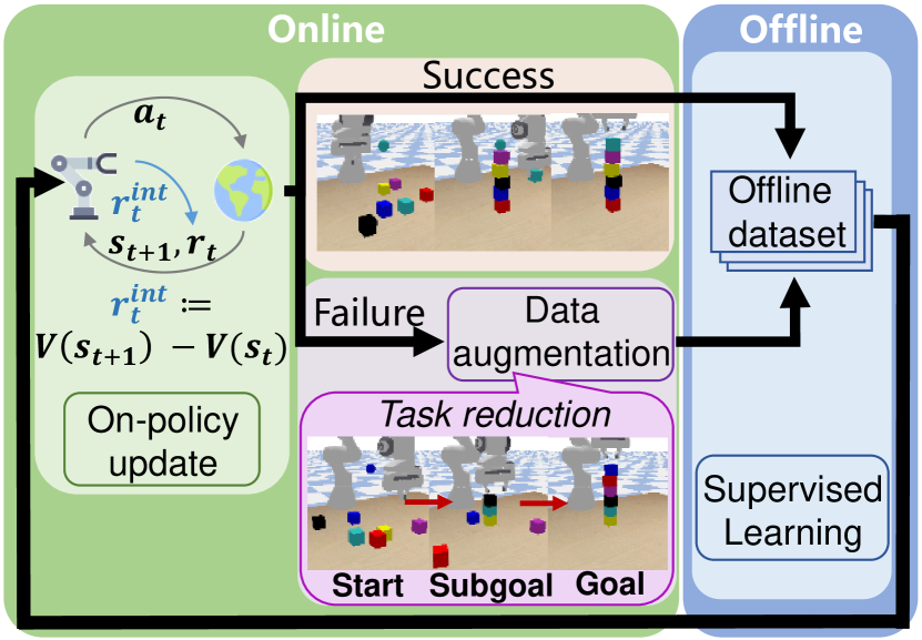
Figure 1: Overall workflow of PAIR. PAIR iteratively alternates between online RL and offline SL phases. During online phases, the agent is trained using both environment reward and a value-difference-based intrinsic reward. Meantime, it collects trajectories and augments them with task reduction into successful demonstrations for offline training. In the offline phases, the agent runs supervised learning to improve its policy using the generated dataset.

One representative line of research that incorporates SL into RL is offline RL, which assumes that a large offline dataset of transition data is available and solely performs learning on the dataset without interacting with the environment (Lange et al., 2012; Wu et al., 2019; Levine et al., 2020; Kumar et al., 2020; Fujimoto & Gu, 2021). However, both empirical (Yu et al., 2021b) and theoretical (Rashidinejad et al., 2021) evidence suggests that the success of recent offline RL methods rely on the quality of the dataset. Accordingly, popular offline RL datasets are typically constructed by human experts, which may not be feasible for many real-world problems. Besides, offline RL suffers from a final performance gap compared with online RL algorithms.

Another representative line of research is self-imitation learning (SIL) (Oh et al., 2018), which combines SL and RL in a completely online fashion. SIL directly performs SL over selected self-generated rollout trajectories by treating the SL objective as an auxiliary loss and optimizing it jointly with the standard RL objective. SIL does not require a dataset in advance. However, optimizing a mixed objective consisting of both RL and SL makes the optimization process even more brittle and requires substantial efforts of parameter tuning to achieve best empirical performance.

In this paper, we propose a simple phasic approach, PhAsic self-Imitative Reduction (PAIR), to effectively balance both RL and SL training for goal-conditioned sparse-reward problems. The main principle of PAIR is to alternate between RL and SL: in the RL phase, we solely perform standard online RL training for optimization stability and collect rollout trajectories as a dataset for the offline SL phase; while in the SL phase, we pick out successful trajectories as SL signals and run imitation learning to improve policy. To improve sample efficiency, PAIR also includes two additional techniques in the RL phase: 1) a value-difference-based intrinsic reward that alleviates the sparse-reward issue, and 2) task reduction, a data augmentation technique that largely increases the total number of successful trajectories, especially for hard compositional tasks. Our theoretical analysis suggests that task reduction can converge exponentially faster than the vanilla phasic approach that does not use task reduction.

We implement PAIR with Proximal Policy Optimization (PPO) for RL and behavior cloning for SL and we conduct experiments on a variety of goal-conditioned control problems, including relatively simple benchmarks such as pushing and ant-maze navigation, and a challenging sparse-reward cube-stacking task. PAIR substantially outperforms all the baselines including non-phasic online methods, which jointly perform self-imitation and RL training, and phasic SL methods, which only perform supervised learning on self-generated trajectories (Ghosh et al., 2020). We highlight that PAIR successfully learns to stack 6 cubes with 0/1 rewards from scratch. To our knowledge, PAIR is the first deep RL method that could solve this challenging sparse reward task.

2 Related Work

Goal-conditioned RL: We study goal-conditioned reinforcement learning (Kaelbling, 1993) with sparse reward in this work. Goal-conditioned RL enables one agent to solve a variety of tasks by predicting actions given both observations and goals, and is studied in a number of works (Schaul et al., 2015; Nair et al., 2018b; Pong et al., 2018; Veeriah et al., 2018; Zhao et al., 2019; Eysenbach et al., 2020). Although some techniques like relabeling (Andrychowicz et al., 2017) are proposed to address the sparse reward issue when learning goal-conditioned policies, there are still challenges in long-horizon problems (Nasiriany et al., 2019).

Offline reinforcement learning: Offline RL (Lange et al., 2012; Levine et al., 2020) is a popular line of research that incorporates SL into RL, which studies extracting a good policy from a fixed transition dataset. A large portion of offline RL methods focus on regularized dynamic programming (e.g., Q-learning) (Kumar et al., 2020; Fujimoto & Gu, 2021), with the constraint that the resulting policy does not deviate too much from the behavior policy in the dataset (Wu et al., 2019; Peng et al., 2019; Kostrikov et al., 2021). Some other works directly treat policy learning as a supervised learning problem, and learn the policy in a conditioned behavior cloning manner (Chen et al., 2021; Janner et al., 2021; Furuta et al., 2021; Emmons et al., 2021), which can be considered as special cases of upside down RL and reward-conditioned policies (Schmidhuber, 2019; Kumar et al., 2019). There are also methods that learn transition dynamics from offline data before extracting policies in a model-based way (Matsushima et al., 2020; Kidambi et al., 2020). Some works also consider a single online fine-tuning phase after offline learning (Nair et al., 2020; Lu et al., 2021; Mao et al., 2022; Uchendu et al., 2022) while we repeatedly alternate between offline and online training.

Imitation learning in RL: Imitation learning is a framework for learning policies from demonstrations, which has been shown to largely improve the sample complexity of RL methods (Hester et al., 2018; Rajeswaran et al., 2018) and help overcome exploration issues (Nair et al., 2018a). Self-imitation learning (SIL) (Oh et al., 2018), which imitates good data rolled out by the RL agent itself, does not require any external dataset and has been shown to help exploration in sparse reward tasks. Our method also performs imitation learning over self-generated data. Self-imitation objective is optimized jointly with the RL objective, while we propose to perform SL and RL separately in two phases. The idea of substituting joint optimization with iterative training for minimal interference between different objectives is similar to phasic policy gradient (Cobbe et al., 2021). Goal-conditioned supervised learning (GCSL) (Ghosh et al., 2020) is perhaps the most related work to ours. GCSL repeatedly performs imitation learning on self collected relabeled data without any RL updates while we leverage the power from both RL and SL and adopt further task reduction for enhanced data augmentation.

Sparse reward problems: There are orthogonal interests in solving long horizon sparse reward with hierarchical modeling (Stolle & Precup, 2002; Kulkarni et al., 2016; Bacon et al., 2017; Nachum et al., 2018) or by encouraging exploration (Singh et al., 2005; Burda et al., 2019; Badia et al., 2020; Ecoffet et al., 2021). Our framework can be also viewed as an effective solution to tackle challenging sparse-reward compositional problems.

3 Preliminary

We consider the setting of goal-conditioned Markov decision process with 0/1 sparse rewards defined by $(\mathcal{S},\mathcal{A},P(s^{\prime}|s,a),\mathcal{G},r(s,a,g),\rho_{0},\gamma)$. $\mathcal{S}$ is the state space, $\mathcal{A}$ is the action space, $\mathcal{G}$ is the goal space and $\gamma$ is the discounted factor. $P(s^{\prime}|s,a)$ denotes transition probability from state $s$ to $s^{\prime}$ after taking action $a$. The reward function $r(s,a,g)$ is 1 only if the goal $g$ is reached at the current state $s$ within some precision threshold and otherwise 0. In the beginning of each episode, the initial state $s_{0}$ is sampled from a distribution $\rho_{0}$ and a goal $g$ is sampled from the goal space. An episode terminates when the goal is achieved or it reaches a maximum number of steps.

The agent is represented as a goal-conditioned stochastic policy $\pi_{\theta}(a|s,g)$ parametrized by $\theta$. The optimal policy $\pi_{\theta^{\star}}$ should maximize the objective $J(\theta)$ defined by the expected discounted cumulative reward over all the goals, i.e.,

$$J(\theta)=J(\pi_{\theta})=\mathbb{E}_{g\in\mathcal{G},a_{t}\sim\pi_{\theta}}\left[\sum_{t}\gamma^{t}r(s_{t},a_{t},g)\right].$$ (1)

Policy gradient optimizes $J(\theta)$ via the gradient computation

$$\nabla J(\theta)=\mathbb{E}_{g,a_{t}}\left[\sum_{t}(R_{t}-V_{\psi}(s_{t},g))\nabla\log\pi(a_{t}|s_{t},g)\right],$$

where $V_{\psi}(s_{t},g)$ is the goal-conditioned value function parameterized by $\psi$ and $R_{t}$ denotes the discounted return starting from time $t$ on the current trajectory. Note that in our goal-conditioned setting with 0/1 rewards, $R_{t}$ will be either 0 or 1 and the value function $V_{\psi}(s_{t},g)$ can be approximately interpreted as the discounted success rate from state $s_{t}$ towards goal $g$.

Goal-conditioned imitation learning optimizes a policy $\pi_{\theta}$ by running supervised learning over a given demonstration dataset $\mathcal{D}=\{\tau:(g;s_{0},a_{0},s_{1},a_{1},\ldots)\}$, where $\tau$ denotes a single trajectory. The supervised learning loss $L(\theta)$ is typically defined by

$$L(\theta)=-\mathbb{E}_{(g;s,a)\in\mathcal{D}}\left[w(s,a,g)\log\pi(a|s,g)\right],$$ (2)

where $w(s,a,g)$ is some sample weight. Behavior cloning (BC) simply sets $w(s,a,g)$ as $1$ while more advanced methods may have other choices. Note that self-imitation learning (SIL) is a paradigm that jointly optimizes the RL objective $J(\theta)$ and the SL objective $L(\theta)$ in an online fashion.

4 Method

Our phasic solution PAIR consists of 3 components, including the online RL phase (Sec. 4.1), which also collects rollout trajectories, task reduction (Sec. 4.2) as a mean for data augmentation, and the offline phase (Sec. 4.3), which performs SL on self-generated demonstrations. We summarize the overall algorithm in Sec. 4.4.

4.1 RL Phase with Intrinsic Rewards

The RL phase follows any standard online RL training. Specifically in our work, we adopt PPO (Schulman et al., 2017) as our RL algorithm, which trains both policy $\pi_{\theta}$ and value function $V_{\psi}$ using rollout trajectories. When a trajectory $\tau=(g;s_{t},a_{t})$ is successful, i.e., goal $g$ is reached, we keep this trajectory $\tau$ as a positive demonstration towards goal $g$ in the dataset $\mathcal{D}$ for the offline phase.

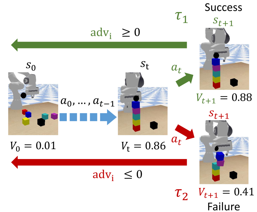
Figure 2: Motivation of value-difference intrinsic reward. Trajectories $\tau_{1}$ and $\tau_{2}$ only differ at a single action $a_{t}$. $\tau_{1}$ succeeds and will have positive advantage. $\tau_{2}$ fails since $a_{t}$ knocks down the cubes, then all the transitions in $\tau_{2}$ will have negative advantages due to 0/1 goal-conditioned reward, even if early actions are perfect.

Value-difference-based intrinsic rewards:

The sparse-reward issue is a significant challenge for online RL training, which can yield substantially high variance in gradients. In particular, let’s assume $\gamma=1$ for simplicity and consider a single trajectory $\tau=(g;s_{t},a_{t})$. In our goal-conditioned setting, the return $R_{t}$ on $\tau$ will be binary and the value function $V_{\psi}(s_{t},g)$ will be approximately between 0 and 1. Hence, the advantage function for state-action pair $(s_{t},a_{t})\in\tau$, i.e., $R_{t}-V(s_{t})$, will be either positive or negative for the entire trajectory $\tau$. Imagine a concrete example as illustrated in Fig. 2, where we have two trajectories, a successful trajectory $\tau_{1}$ and a failed trajectory $\tau_{2}$. These two trajectories only differ at the final timestep $s_{t+1}$, which may be due to some random exploration noise at action $a_{t}$. However, only due to a single mistake, all the state-action pairs from $\tau_{2}$ will have negative advantages, even though most of the actions in $\tau_{2}$ are indeed approaching the desired target. Likewise, in a successful trajectory, it is also possible that some single action is poor but eventually the subsequent actions fix this early mistake.

Besides the trajectory-based advantage computation, it will be beneficial to have some effective signal of whether a transition $(s_{t},a_{t},s_{t+1})$ is properly “approaching” the desired goal $g$ or not. Our suggestion is to use $V_{\psi}(s,g)$ as an empirical measure: if $a_{t}$ is a good action, it should lead to a higher state value, i.e., $V_{\psi}(s_{t+1},g)-V_{\psi}(s_{t},g)>0$, which indicates that $a_{t}$ moves to a state with a higher success rate; similarly, a poor action will result in a value drop, i.e., $V_{\psi}(s_{t+1},g)-V_{\psi}(s_{t},g)<0$. Accordingly, we propose to adopt value difference as an intrinsic reward $r^{\textrm{int}}$ for stabilizing goal-conditioned RL training as follows

$$r^{\textrm{int}}(s_{t},a_{t},g):=V_{\psi}(s_{t+1},g)-V_{\psi}(s_{t},g).$$

We remark that $r^{\textrm{int}}$ relies on an accurately learned value function $V_{\psi}(s,g)$. Therefore, we suggest to only train $V_{\psi}(s,g)$ over the sparse goal-conditioned rewards while using another value head to fit the intrinsic rewards for critic learning. Similar techniques have been previously explored in (Burda et al., 2019) as well.

4.2 Task Reduction as Data Augmentation

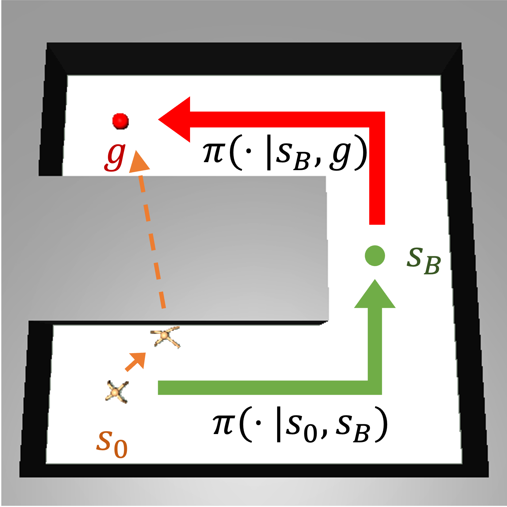
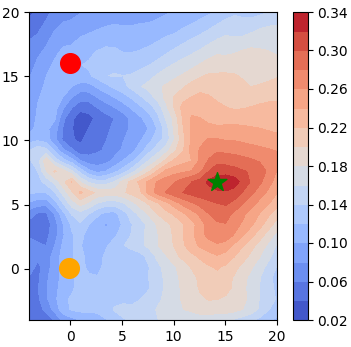
Figure 3: Illustration of task reduction. (Left) Given a trajectory that fails to reach $g$ from $s_{0}$ (orange arrows), task reduction searches for an intermediate $s_{B}$, then executes the resulting two sub-tasks (green and red arrows) to generate a successful demonstration. (Right) Heatmap of composed value in Eq. 4 w.r.t. $s_{B}$. The green star denotes the position of optimal $s_{B}$.

In order to perform effective supervised learning in the offline phase, it is critical that the online phase can generate as much successful trajectories as possible. In our framework, we consider two data augmentation techniques to boost the positive samples in the dataset $\mathcal{D}$, i.e., goal relabeling and task reduction. We will first describe the simpler one, goal relabeling, before moving to a much more powerful technique, task reduction.

Goal relabeling was originally proposed by Andrychowicz et al. (2017). In our goal-conditioned learning setting, for each failed trajectory $\tau=(g;s_{t},a_{t})$ originally targeted at goal $g$, we can create an artificial goal $g^{\prime}$ by setting $g^{\prime}=s_{j}$ for some reached state $s_{j}\in\tau$, which naturally yields a successful trajectory $\tau^{\prime}$ as follows:

$$\tau^{\prime}\leftarrow(g^{\prime}=s_{j};s_{t=0:j},a_{t=0:j})\quad\textrm{where}\;\;s_{j}\in\tau.$$ (3)

Therefore, despite its simplicity, goal relabeling can convert every failed trajectory $\tau$ to a positive demonstration without any further interactions with the environment.

Task reduction was originally proposed by Li et al. (2020b). The main idea is to decompose a challenging task into a composition of two simpler sub-tasks so that both sub-tasks can be solved by the current policy. As illustrated in the left part of Fig. 3, given a goal $g$ from state $s_{0}$, task reduction searches for the best sub-goal $s_{B}^{\star}$ through a 1-step planning process over the universal value function $V_{\psi}(s,g)$ as follows

$$s_{B}^{\star}=\arg\max_{s_{B}}V_{\psi}(s_{0},s_{B})\oplus V_{\psi}(s_{B},g),$$ (4)

where $\oplus$ is a composition operator typically implemented as multiplication. Since the value function is learned, such a search process can be accomplished without any further environment interactions by gradient descent or cross-entropy method. A heatmap of the composed value for sub-goal search (Eq.(4)) is visualized in the right part of Fig. 3. Notably, after $s_{B}^{\star}$ is obtained, we would still need to execute the policy in the environment following the sub-goal $s_{B}^{\star}$ and then the final goal $g$ in order to obtain a valid demonstration. Compared to goal relabeling, task reduction consumes additional samples and may even fail to produce a successful trajectory when either of the two sub-tasks fails. Hence, task reduction can be expensive in the early stage of training when the policy and value function have not yet been well trained. However, we will show both theoretically (Sec. 5) and empirically (Sec. 6.2) that task reduction can lead to an exponentially faster convergence compared to using goal relabeling solely in long-horizon problems.

By default, PAIR utilizes both goal relabeling and task reduction for data augmentation unless otherwise stated.

4.3 Offline SL Phase

After a dataset $\mathcal{D}$ of successful demonstrations, including augmented trajectories, is collected, we switch from RL training to offline SL by performing advantage weighted behavior cloning (BC). In particular, we set the weight $w(s,a,g)$ in Eq. (2) to $\exp{(\frac{1}{\beta}(R-V_{\phi}(s,g)))}$ following (Peng et al., 2019). We remark that we only train policy in the offline phase while keeping the value function $V_{\psi}$ unchanged for algorithmic simplicity. We also empirically find that training value function during the offline phase does not improve the overall performance.

It is feasible to adopt more advanced methods in the offline phase, such as offline RL methods, which typically assume a pre-constructed dataset but conceptually compatible with our phasic learning process. We conduct experiments by substituting BC with two popular offline RL methods, decision transformer (Chen et al., 2021) and AWAC (Nair et al., 2020), in Sec. 6.1. Empirical results show that these alternatives are much more brittle than BC and perform poorly without a high-quality warm-start dataset. Thus, we simply use BC as our SL method in this paper.

4.4 PAIR: Phasic Self-Imitative Reduction

By repeatedly performing the online RL phase with task reduction and the offline SL phase, we derive our final algorithm, PAIR. The pseudo-code is summarized in Alg. 1. More implementation details can be found in Appendix B.3. More analysis on the phasic training scheme vs. joint RL and SL optimization is in Appendix B.4.

Algorithm 1 Phasic Self-Imitative Reduction

1:  Initialize: goal-conditioned policy $\pi_{\theta}(\cdot|s,g)$, value function $V_{\psi}(s,g)$.

2:  for $k\leftarrow 1,2,\cdots$ do

3:     Sample a batch of trajectories $\mathcal{B}\leftarrow\{\tau:(g;s_{t},a_{t})\}$ w.r.t. the current policy $\pi_{\theta}$

4:     Update $\pi_{\theta},V_{\psi}$ by RL on $\mathcal{B}$ (Sec. 4.1)

5:     Set dataset $\mathcal{D}\leftarrow\emptyset$

6:     for $\tau\in\mathcal{B}$ do

7:        if not is_success($\tau$) then

8:           $\tau\leftarrow\texttt{data\_augment}(\tau,\pi_{\theta},V_{\psi})$ (Sec. 4.2)

9:        end if

10:        $\mathcal{D}\leftarrow\mathcal{D}\cup\{\tau\}$

11:     end for

12:     Train $\pi_{\theta}$ with SL over $\mathcal{D}$ (Sec. 4.3)

13:  end for

5 Theoretical Analysis

First, we establish the correctness of our framework. The following theorems follows directly from the GCSL framework in (Ghosh et al., 2020), because both GCSL and PAIR are built upon SL.

Theorem 5.1 (Ghosh et al. (2020), Theorem 3.1).

Let $J(\pi)$ be defined in Eq. (1) and $J_{\mathrm{PAIR}}(\pi)=-L(\theta)$ as defined in Eq. (2). Let $\tilde{\pi}$ be the data collection policy induced by data augmentation. Then

$$J(\pi)\geq J_{\mathrm{PAIR}}(\pi)-4T(T-1)\alpha^{2}+C,$$ (5)

where $\alpha=\max_{s,g}D_{\mathrm{TV}}(\pi(\cdot|s,g)\|\tilde{\pi}(\cdot|s,g))$ and $C$ is a constant independent of $\pi$.

Theorem 5.2 (Ghosh et al. (2020), Theorem 3.2).

Assume deterministic transition and that $\tilde{\pi}$ has full support. Define

$$\epsilon:=\max_{s,g}D_{\mathrm{TV}}(\pi(\cdot|s,g)\|\hat{\pi}^{\star}(\cdot|s,g)).$$ (6)

Then $J(\pi^{\star})-J(\pi)\leq\epsilon\cdot T$, where $\hat{\pi}^{\star}$ minimizes $L(\theta)$ defined in Eq. (2) and $\pi^{\star}$ is the optimal policy.

Here, we present theoretical justification to illustrate why our algorithm is efficient on sparse-reward composite combinatorial tasks.

Theorem 5.3.

Under mild assumptions, the PAIR framework could use exponentially less number of iterations compared to the phasic framework that does not use task reduction, e.g., GCSL (Ghosh et al., 2020).

We defer the exact statement of Theorem 5.3 and its proof to Appendix A.

6 Experiment

We aim to answer the following questions in this section:

• Does phasic training of RL and SL objectives perform better than non-phasic joint optimization?

• Is PAIR compatible with offline RL methods other than BC?

• Does PAIR achieve exponential improvement over baselines without task reduction?

• Are all the algorithmic components of PAIR necessary for good performance?

• Can PAIR be used to solve challenging long-horizon sparse-reward problems, e.g., cube stacking?

We consider 3 goal-conditioned control problems with increasing difficulty: (i) short-horizon robotic pushing (adopted from (Nair et al., 2018b)), (ii) ant navigation in a U-shaped maze, and (iii) robotic stacking with up to 6 cubes. All the tasks are with only 0-1 sparse reward.

We compare PAIR with non-phasic RL baslines that jointly perform RL and SL as well as phasic SL baselines that only perform SL over self-generated data. For non-phasic RL baselines, we consider naive PPO, plain self-imitation learning with goal relabeling (SIL) (Oh et al., 2018) and self-imitation learning with task reduction (SIR) (Li et al., 2020b). For phasic SL baselines, we consider goal-conditioned supervised learning (GCSL) (Ghosh et al., 2020). We emphasize that for a fair comparison, all the RL-based baselines leverage our proposed intrinsic rewards. All the experiments are repeated over 3 random seeds on a single desktop machine with a GTX3090 GPU. More implementation and experiment details can be found in appendix.

6.1 Sawyer Push

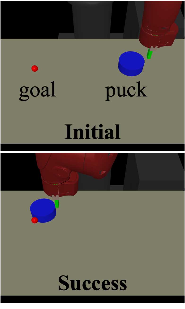
Figure 4: An initial state and a successful state in “Push” environment.

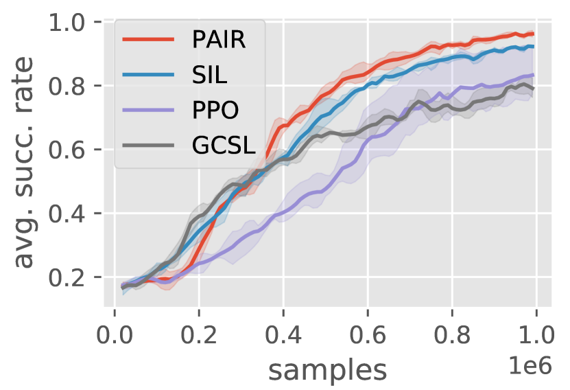
Figure 5: Average success rate vs. number of samples in “Push”. PAIR achieves the best performance compared to non-phasic, pure RL and pure SL baselines.

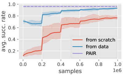
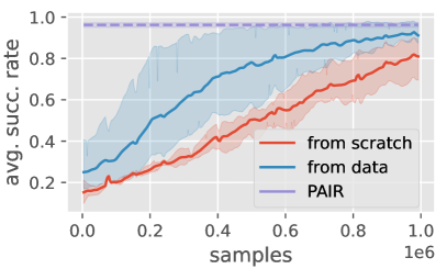
Figure 6: Combining PAIR with offline algorithms AWAC (left) and DT (right) in “Push” domain. We train them both from scratch (red) and from a demonstration dataset (blue). The performances of PAIR with PPO/BC are in dashed purple line.

We first answer whether our phasic framework can outperform non-phasic training algorithms on a simple “Push” task. As illustrated in Fig. 5, a Sawyer robot is tasked to push the puck to the goal within 50 steps. The initial position of the robot hand, the puck and the goal are randomly initialized on the table. Since it only requires very few steps to reach the goal – even the largest distance between puck and goal is within 20 steps of actions using a well trained policy, task reduction would not make its best use and may hurt sample efficiency due to extra sample consumption. In this particularly simple domain, we only use goal relabeling as a single data augmentation technique in PAIR.

Effectiveness of phasic training: We compare PAIR with non-phasic RL method, i.e., SIL, which utilizes the successful relabeled demonstrations by jointly optimizing SL and RL objectives. As shown in Fig. 5, PAIR (red) gets higher success rate than SIL (blue) using fewer samples while both methods perform better than naive PPO, which is a pure RL baseline. We also compare with phasic SL method, GCSL (Ghosh et al., 2020), which only performs iterative SL on relabeled data without RL training. Following the original implementation of GCSL, every trajectory is relabeled as a successful one targeting at an achieved state. GCSL learns fast in the beginning, but achieves a substantially lower final success rate than other methods.

Combining with offline RL methods: Here we provide the results with initial attempts to combine our framework with representative offline RL methods, AWAC (Nair et al., 2020) and decision transformer (DT) (Chen et al., 2021).

Original AWAC performs a single fine-tuning phase after offline pretraining (Nair et al., 2020; Lu et al., 2021). Following the phasic framework of PAIR, we alternate between offline and online AWAC updates. We examine both training from scratch without any dataset prepared in advance, or starting from the offline phase with a warm-start dataset of successful trajectories. The results are shown on the left of Fig. 6. Phasic-AWAC from scratch (red) continues making progress as it switches from offline to online phase, but finally converges to a much worse policy compared with the variant initialized with a warm-start dataset (blue).

DT predicts actions conditioning on a sequence of desired returns, past states and actions via a transformer model (Vaswani et al., 2017). Since DT is proposed only for a single offline phase, we similarly adopt PPO for RL training in the online phase. We use a context length of 5 for sequence conditioning and train DT both from scratch and from prepared warm-start dataset with successful demonstrations. As shown in the right plot of Fig. 6, the performance progressively improves within each online phase and SL phase. Phasic-DT with warm-start (blue) outperforms the variant from scratch and gets similar final performance as PAIR but the variance is much higher.

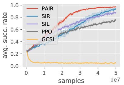
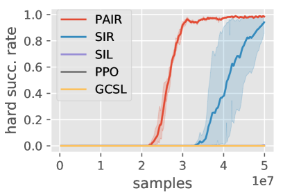
Figure 7: (Left) Average success rate over uniformly sampled tasks, where ant and goal positions are uniformly sampled. (Right) Success rate evaluated on one particularly difficult task configuration with ant and goal initialized at two ends of the maze.

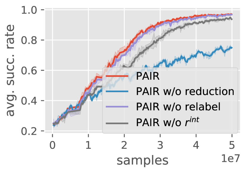
(a) Ablate PAIR components.

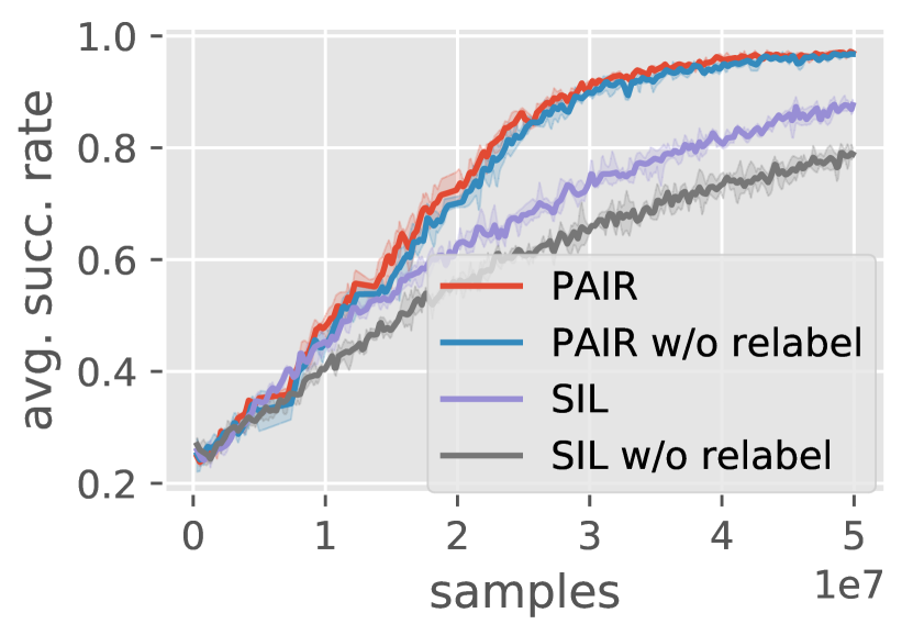
(b) The effect of goal-relabeling on SIL.

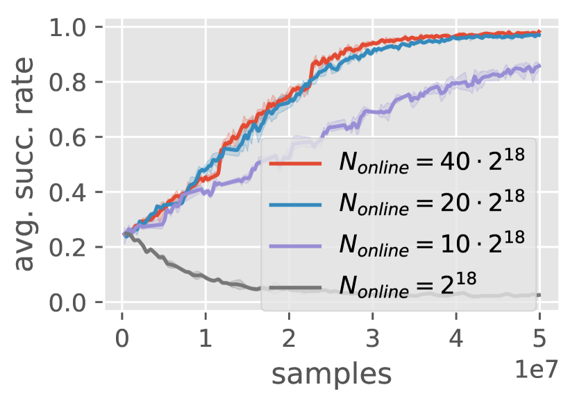
(c) Sensitivity analysis of $N_{\textrm{online}}$.

Figure 8: Ablation studies on algorithmic components of PAIR in “Ant Maze”. (a) Performances after removing different components of PAIR. Using reduction data and intrinsic reward help the most for PAIR. (b) Validate the effectiveness of goal relabeling on SIL. (c) Comparison of different $N_{\textrm{online}}$, i.e., samples collected in the RL phase. PAIR works well with less frequent phase switches.

We generally observe that offline RL algorithms within our phasic framework would require a good dataset to initialize and do not perform as robustly as the simple PPO and BC combination when starting from scratch. Therefore, we confirm our use of BC/PPO for the remaining experiments and leave a more competitive combination with offline RL algorithms as future work.

6.2 Ant Maze

We then consider a harder task “Ant Maze”, which requires a locomotion policy with continuous actions to control the ant robot and plan over an extended horizon to navigate inside a 2-D U-shape maze. The observations include the center of mass and the joint position and velocities of the ant robot. The goal is a 2-D vector denoting the $xy$ position of that the robot should navigate to. For each episode, the initial position of the ant’s center and the goal position are uniformly sampled over the empty space inside the maze. We define the hard task configuration as when the ant and the goal are initialized at two different ends of the maze (see Fig. 3). In this domain, we leverage both task reduction and goal relabeling as data augmentation techniques in PAIR.

Effectiveness of PAIR and exponential improvement on hard goals: As shown in Fig. 7, we evaluate the performances of different algorithms with the average success rate over the entire task space (left) and on hard tasks only (right). We compare PAIR with: SIR, which runs SL and RL jointly using both reduction and relabeling data; SIL, a plain non-phasic RL method without task reduction; GCSL and vanilla PPO. We observe that all the methods that utilize task reduction (i.e., PAIR, SIR) can finally converge to a much higher average success rate (left plot) and outperform SIL and vanilla PPO. The gap becomes substantially larger on the performance on hard situations (right plot), where only methods with task reduction are able to produce non-zero success rate within the given sample budget. This empirical observation is consistent with our theoretical analysis in Sec. 5 on the effectiveness of task reduction. We also remark that PAIR achieves a significantly higher sample efficiency compared with the non-phasic method SIR on the hard cases. Notably, GCSL completely fails in this problem. We empirically observe that the ant robot may frequently get stuck in the early stage of training (e.g., it may accidentally fall over and cannot recover anymore). We hypothesis that the failure of GCSL is largely due to a tremendous amount of supervision from such corrupted trajectories. This suggests that online RL training would be necessary compared with running SL only (e.g., SIL performs well on this task).

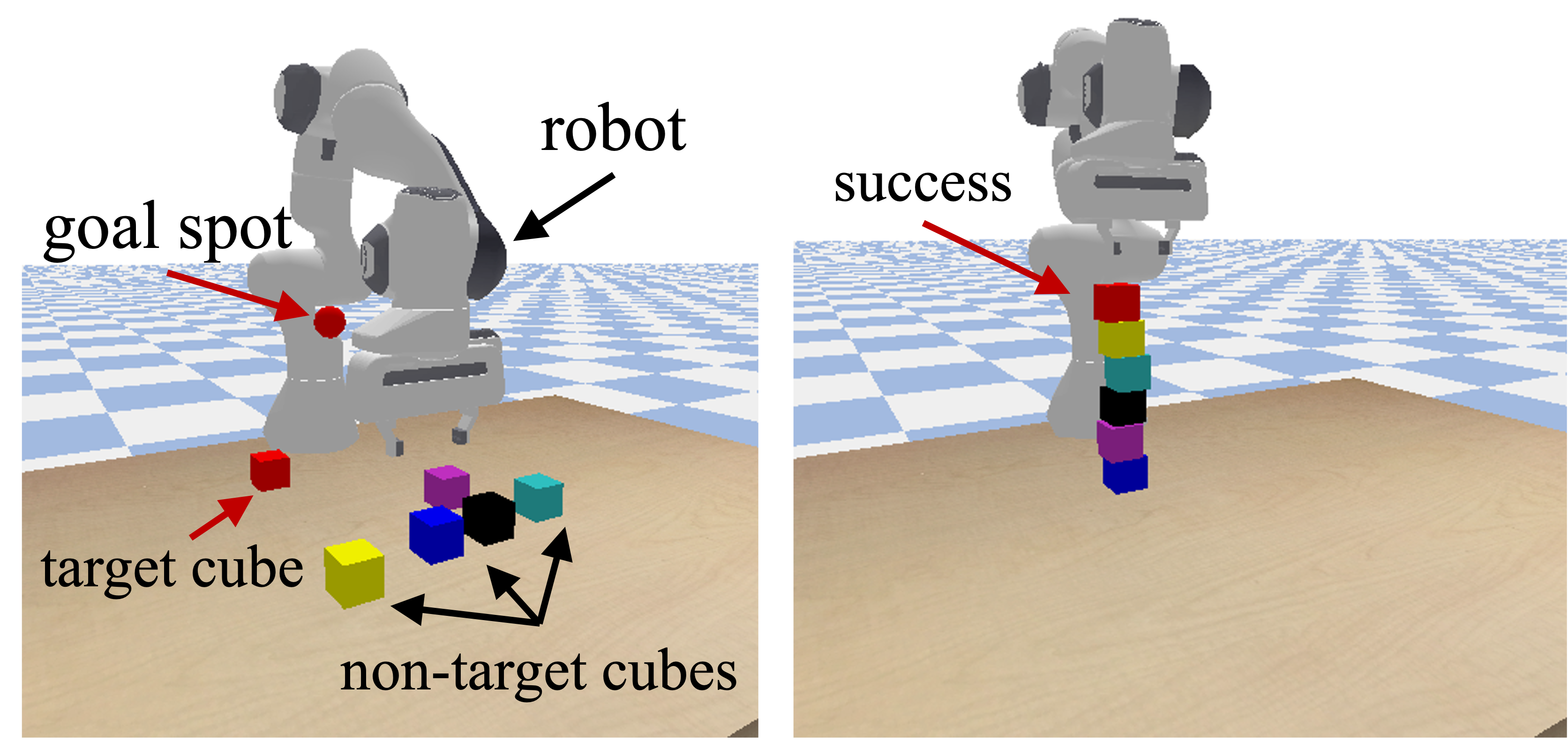
Figure 9: Illustration of the stacking environment. The left figure shows an initial state, where the red ball denotes the identity and the desired position of a target cube. On the right we show a successful state for this task, where the red cube is close to the goal and the robot hand does not touch the tower.

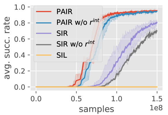
Figure 10: Average success rate in “stack-6-cube” with sparse reward. PAIR solves the task with high success rate most efficiently.

Algorithm	SR @ 7.5e7 steps	SR @ 1.5e8 steps
PAIR	0.693 $\pm$ 0.176	0.955 $\pm$ 0.005
PAIR w/o $r^{\textrm{int}}$	0.493 $\pm$ 0.156	0.952 $\pm$ 0.016
SIR	0.026 $\pm$ 0.043	0.815 $\pm$ 0.039
SIR w/o $r^{\textrm{int}}$	0.003 $\pm$ 0.003	0.688 $\pm$ 0.011
SIL	0.000 $\pm$ 0.000	0.000 $\pm$ 0.000

Figure 11: Mean and standard deviation of success rates for stacking 6 boxes with different algorithms over 3 seeds. The policies are evaluated at 7.5e7 and 1.5e8 environment samples.

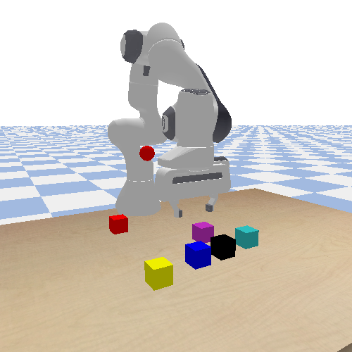
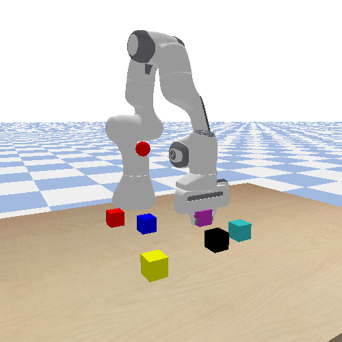
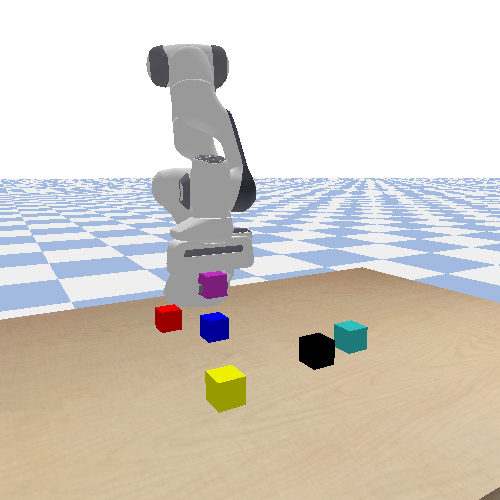
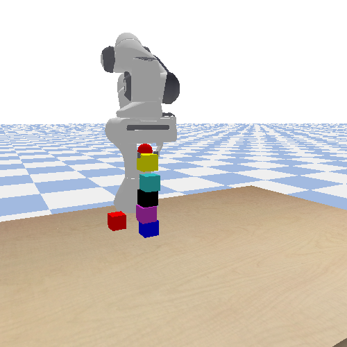
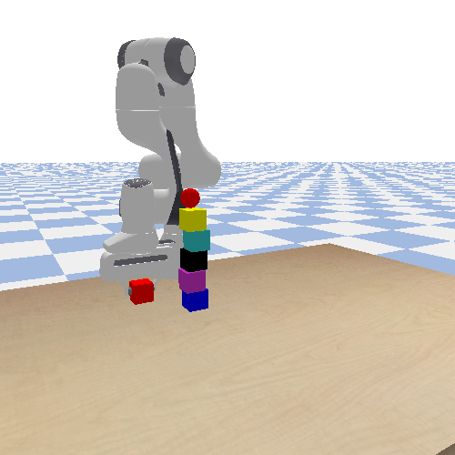
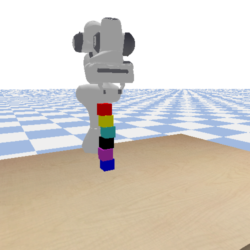
Figure 12: Learned policy of PAIR agent for stacking 6 randomly initialized cubes.

Ablation studies: We then study the effectiveness of different components of PAIR. From Figure 8(a), we can find that removing value-difference-based intrinsic reward makes PAIR converge slower while the policy is still able to achieve a high success rate after convergence. After removing task reduction, the performance becomes significantly worse. By contrast, when removing goal relabeling, the performance drop is negligible. These observations suggest that task reduction is the most critical component in PAIR. In Figure 8(b), we additionally examine the effectiveness of goal relabeling within a non-phasic RL framework, i.e., SIL, where we can clearly observe a performance drop of SIL with goal relabeling turned off. This indicates that goal relabeling can be still beneficial for methods that do not utilize task reduction. Finally, in Figure 8(c), we also perform sensitivity analysis on the frequency of alternating between the offline and online phase. We perform one offline SL phase after collecting $N_{\textrm{online}}$ samples in the online RL phase. We can observe that a relatively low alternating frequency is critical to the success of PAIR, which suggests that a large dataset for SL training and a long RL fine-tuning period help accelerate learning. We notice that when the phase changes too frequently, PAIR can be unstable or even fail to learn.

6.3 Stacking

Finally, we test whether PAIR can solve an extremely challenging long-horizon sparse-reward robotic manipulation problem. We build a robotic control environment that features stacking multiple cubes given only final success reward. The simulated scene is shown in Fig. 9. A Franka Panda arm is mounted on the side of a table. On top of the table, there are a total of $N$ cubes with random initial positions. A goal spot specifies a target cube using its color and also its desired position. The robot’s task is to manipulate the cubes on the table so that the specified target cube can remain stable within 3cm distance to the goal position, while its hand is at least 10cm apart from that position at the same time. In order to accomplish this task, the robot must build a “base” tower using other non-target cubes. During the whole construction process, the robot cannot receive any external reward for intermediate manipulations unless when the target cube is in place. We perform curriculum on the number of cubes to stack, and use the similar task reduction process described in (Li et al., 2020b). More details of training specifications can be found in Appendix B.1.3.

Performance on stacking with 6 cubes: We report the success rate on the most challenging “stack-6-cube” scenario using PAIR, SIR and SIL algorithms in Fig. 11 and Table 11. PAIR achieves an impressive 95.5% success rate in this challenging task. SIR is making considerable progress thanks to task reduction, but it learns significantly less sample efficiently than PAIR. SIL baseline without task reduction fails completely, getting 0 success rate throughout the training process. We also show the effectiveness of intrinsic reward in online training: similar to the findings in other domains, $r^{\textrm{int}}$ can significantly speed up the training process.

Learned strategies: The learned policy using PAIR is visualized in Fig. 12. In the initial frame, all 6 cubes are scattered randomly on the table. The robot then picks up non-target cubes, transports them to accurate positions aligned with the goal spot one by one. Even when picking up the red cube which locates close to the half-built tower, the robot is cautious enough to avoid knocking down the tower.

7 Conclusion

We propose a phasic training method PAIR that efficiently combines offline supervised learning with online reinforcement learning for sparse-reward goal-conditioned problems, such as robotic stacking of multiple cubes. PAIR repeatedly alternates between SL on self-generated datasets and RL fine-tuning and leverages value difference as intrinsic rewards and task reduction as data augmentation. We validate the effectiveness of PAIR both theoretically and empirically on a variety of domains. We remark that PAIR provides a general learning paradigm that has the potential to be combined with more advanced offline RL methods, even though our initial attempts are not satisfactory. We hope PAIR can be a promising step to take advantage of both supervised learning and reinforcement learning and help make RL a more scalable tool for complex real-world challenges.

The project webpage is at https://sites.google.com/view/pair-gcrl.

Appendix A Missing Proofs in Section 5

In this section, we prove Theorem 5.3.

Here, we make the following assumptions to facilitate our analysis. First, we consider a goal-conditioned MDP with deterministic transition. We assume that the goal set is the same as the state space, i.e., $\mathcal{G}=\mathcal{S}$. Furthermore, we consider sparse-reward environment where the reward function is defined by $r(s,a,g)=\mathbb{I}\{s=g\}$.

We note that our framework draw on-policy trajectories with random state-goal pairs. To further simplify our theoretical analysis, we assume that each state-goal pair is sampled at least once in each iteration. Here, we may meet two practical issues. First, the state space may be continuous, which makes it impossible to sample each state-goal pair once. This may fit into our theoretical analysis by discretizing the state space. Second, $N_{\mathrm{online}}$ may not be large enough. This fits into our analysis by merging several consecutive iterations.

We use $\pi^{(k)}$ to denote the policy by the end of the $k$-th iteration, and $\pi^{(0)}$ denotes the initial policy. We assume that the initial policy $\pi^{(0)}$ can reach any one-step goal. Specifically, if $P(s^{\prime}|s,a)=1$ then $\pi^{(0)}(a|s,g=s^{\prime})=1$.

For a state $s$, a goal $g$, and a (deterministic) policy $\pi$, we define

$$s\xrightarrow{\pi}g:=\begin{cases}\text{true},&\Pr[\exists t\geq 0:s_{t}=g\mid s_{0}=s,\forall i\geq 0,a_{i}\sim\pi(\cdot|s_{i},g),s_{i+1}\sim P(\cdot|s_{i},a_{i})]=1,\\ \text{false},&\text{otherwise}.\end{cases}$$ (7)

and we define

$$d(s,s^{\prime}) :=\min\{t:\exists\mathrm{policy}\pi\text{ such that }\Pr[s_{t}=s^{\prime}\mid s_{0}=s,\forall i\geq 0,a_{i}\sim\pi(\cdot|s_{i},g),s_{i+1}\sim P(\cdot|s_{i},a_{i})]=1\},$$ (8)

$$\ell_{k} :=\sup_{\ell}\{\forall s,g:d(s,g)\leq\ell:s\xrightarrow{\pi^{(k)}}g\text{ is true}\}.$$ (9)

Finally, we let

$$D=\max_{s,s^{\prime}\in\mathcal{S}}\{d(s,s^{\prime}):d(s,s^{\prime})<+\infty\}$$ (10)

be the maximum possible length of trajectory from state $s$ to goal $s^{\prime}$ such that $s^{\prime}$ is reachable from $s$.

Lemma A.1.

For the PAIR framework, we have $\ell_{k}\geq 2\ell_{k-1}$ for every iteration $k$.

Proof.

We prove by induction. For every state-goal pair $s,g$ such that $d(s,g)\leq 2\ell_{k-1}$, we can find some state $s^{\prime}$ such that $d(s,s^{\prime})\leq\ell_{k-1}$ and $d(s^{\prime},g)\leq\ell_{k-1}$. By the inductive hypothesis, we have that $s\xrightarrow{\pi^{(k)}}s^{\prime}$ and $s^{\prime}\xrightarrow{\pi^{(k)}}g$ are true.

Now we claim that every $(s,g)\in\mathcal{S}\times\mathcal{G}$ would have a success trajectory after the $k$-th iteration. Note that by our assumption, the framework would roll out a trajectory from $s$ to $g$ using $\pi(\cdot|s,g)$. If it succeeds, then we get a trajectory, else task reduction (cf. Section 4.2) would find the state $s^{\prime}$ such that $s\xrightarrow{\pi^{(k-1)}}s^{\prime}$ and $s^{\prime}\xrightarrow{\pi^{(k-1)}}g$ are true, because $V(s,s^{\prime})=V(s^{\prime},g)=1$. Therefore, task reduction would run $\pi^{(k-1)}(\cdot|s,g=s^{\prime})$ followed by $\pi^{(k-1)}(\cdot|s^{\prime},g)$, and get a successful trajectory from $s$ to $g$. Finally, the SL step would learn the policy $\pi^{(k)}$ such that $s\xrightarrow{\pi^{(k)}}g$ is true. ∎

Lemma A.2.

The PAIR framework uses at most $O(\lvert\mathcal{S}\rvert^{2}\log D)$ samples to learn a policy that could go from any state to any reachable goal.

Proof.

By the definition of $\ell_{k}$, we know that $\pi^{(k)}$ could go from any state to any reachable goal if $\ell_{k}\geq D$. By our assumption, we have $\ell_{0}=1$. Therefore, by Lemma A.1, we have $\ell_{k}\geq D$ after $k=O(\log D)$, i.e., PAIR uses at most $O(\log D)$ iterations.

By our assumption, PAIR uses $O(\lvert\mathcal{S}\rvert\lvert\mathcal{G}\rvert)=O(\lvert\mathcal{S}\rvert^{2})$ samples, because each state-goal pair is sampled for constant number of times. Thus we conclude that PAIR uses at most $O(\lvert\mathcal{S}\rvert^{2}\log D)$ samples in total. ∎

Lemma A.3.

Without PAIR, under assumptions described in Appendix A, for hard tasks, with high probability, the algorithm needs $\Omega(\lvert\mathcal{S}\rvert^{2}D)$ samples to learn a policy that could go from any state to any reachable goal.

Proof.

We consider the following hard task. Suppose $s_{0},a_{0},\cdots,s_{D}$ is a trajectory of length $D$ that maximizes Eq. (10). We assume that the initial policy $\pi^{(0)}$ is a uniformly random policy and we assume $\Pr[\pi^{(0)}(\cdot|s_{i},g=s_{D})]]\propto\lvert\mathcal{A}\rvert^{-1}$ for $i\leq D-2$. We observe that for the SL framework, if $s_{i}\xrightarrow{\pi^{(k)}}s_{D}$ is true then the dataset must contain a trajectory from $s_{i}$ to $s_{D}$, and thus the policy $\pi^{(k)}$ learned by SL would satisfy $s_{j}\xrightarrow{\pi^{(k)}}s_{D}$ for every $j\geq i$. For this, we analyze the sample complexity by analyzing how many iterations would be enough for the algorithm to learn a policy from state $s_{0}$ to goal $s_{D}$. To facilitate analysis, we define $i^{(k)}$ to be the smallest number such that $s_{i^{(k)}}\xrightarrow{\pi^{(k)}}s_{D}$. Then the algorithm learns the desired policy after $k$ iterations only if $i^{(}k)=0$.

Next, we prove that $\mathbb{E}[i^{(k-1)}-i^{(k)}|i^{(k-1)}]\leq O(1)$. To change $i^{(k-1)}$, the algorithm must roll out a success trajectory with goal $s_{D}$ from some $s_{j}$ with $j\leq i$. Note that

$$\Pr[i^{(k-1)}-i^{(k)}=j|i^{(k-1)}] \leq\Pr[\text{algorithm rolls out a success trajectory from }s_{i^{(k-1)}-j}\text{ to }s_{D}]$$ (11)

$$\leq\Pr[\pi^{(k-1)}\text{ could go from }s_{i^{(k-1)}-j}\text{ to }s_{i^{(k-1)}}]$$ (12)

$$\leq O(\lvert\mathcal{A}\rvert^{-j}),$$ (13)

so

$$\mathbb{E}[i^{(k-1)}-i^{(k)}|i^{(k-1)}] =\sum_{j=0}^{i^{(k-1)}}j\cdot\Pr[i^{(k-1)}-i^{(k)}=j|i^{(k-1)}]$$ (14)

$$\leq O(\sum_{j=0}^{\infty}j\cdot\lvert\mathcal{A}\rvert^{-j})$$ (15)

$$\leq O(\lvert\mathcal{A}\rvert^{-1})$$ (16)

$$\leq O(1).$$ (17)

Therefore, by the Azuma-Hoeffding inequality (Azuma, 1967), we conclude that with high probability $1-\delta$, we have $i^{(k)}<D$ for $k=\Theta(D-\sqrt{D\log\delta^{-1}})\geq\Omega(D)$, i.e., $k\geq\Omega(D)$ with high probability. Together with that $\lvert\mathcal{S}\rvert^{2}$ trajectories are rolled out in each iteration, we conclude that the sample complexity is with high probability at least $\Omega(\lvert\mathcal{S}\rvert^{2}D)$. ∎

Finally, we conclude Theorem 5.3 by collecting Lemmas A.2 and A.3.

Appendix B Experiment Details

B.1 Environment Description

In this section, we describe all the environment-specific details regarding MDP definitions.

B.1.1 Sawyer Push

“Push” is a robotic pushing environment adopted from (Nair et al., 2018b) simulated with MuJoCo (Todorov et al., 2012) engine. Each episode lasts for at most 50 steps.

Observation: The agent can observe 2-D hand position and 2-D puck position in each step.

Action space: An action is a 2-D vector denoting the relative movement of the robot hand. The height of the hand and the state of the gripper are fixed. Each dimension ranges from -1 to 1, and is categorized into 3 bins (therefore, there are a total of 9 different actions).

Goal and reward: The puck goal is a 2-D vector denoting the target position on the table. The agent can only get reward when the $l2$ distance between puck and goal is smaller than 5cm.

Initial state: Each episode starts with the hand initialized in a 0.03m $\times$ 0.03m region on the right side of the table, the puck initialized in a 0.07m $\times$ 0.07m square, and the goal is uniformly sampled in a 0.4m $\times$ 0.4m square on the table.

B.1.2 Ant Maze

This environment is adopted from (Nachum et al., 2018). The scene is a 24m $\times$ 24m maze simulated with MuJoCo (Todorov et al., 2012). The maximum number of steps for each episode is 500 steps.

Observation: Joint positions and joint velocities of the ant robot. The center of mass of the robot is included in the joint positions.

Action: 8-D real-valued vector controlling the motors on the robot. The actions output from the policy network are clipped to -30 to 30 before sent to the simulator.

Goal and reward: The goals are 2-D vectors denoting the desired $xy$ position of the ant. The agent gets reward when the distance between the ant’s center of mass and the goal is smaller than 2m.

Initial state: Both the ant and the goal are uniformly sampled in the empty space (not collided with walls) in the maze. For hard tasks, the ant is initialized at coordinate (0m, 0m), and the goal is at coordinate (0m, 16m).

B.1.3 Stacking

The stacking environment is built with PyBullet (Coumans & Bai, 2016).

Observation: The observation is a concatenation of robot state and objects states. The robot state contains 6-D end effector pose, 3-D end effector linear velocity, 1-D finger position, and 1-D finger velocity. Each object state consists of its 6-D pose, 3-D relative position to the robot’s end effector, 3-D linear velocity, 3-D angular velocity and 1-D 0/1 indicator denoting the identity of the target cube.

Action: A concatenation of 3-D relative movement of the end effector and 1-D finger control signal. Each dimension is discretized into 20 bins.

Goal and reward: A goal specifies a 3-D desired position and an identity denoting which cube must be close to the goal spot. A non-zero reward is only given when the target cube is within 3cm distance to the goal, and when the end effector is at least 10cm away from the goal.

Adaptive curriculum: Since directly training on stacking tasks with large number of objects pose severe exploration challenges, we adopt a simple curriculum on the number of cubes to stack, similar to the one in (Li et al., 2020a). In the beginning, 70% of the tasks only need to stack one cube, and the other tasks are uniformly sampled to stack 2 to $N$ cubes. Whenever the average success rate reaches 0.6, the curriculum proceeds from sampling “stack-$n$-cubes” with 70% probability to “stack-($n+1$)-cubes” tasks. We switch to offline SL training when the curriculum proceeds and the success rate for stacking $n+1$ cubes is lower than 0.5.

B.2 Combination with Offline RL

B.2.1 Offline RL combination in Sawyer Push

For the warm-start dataset, we collect rollout trajectories generated by random policy, where we keep successful samples and do goal relabelling on failed trajectories. Therefore, the dataset only consists of successful demonstrations. The dataset size for phasic-DT is $55K$ steps, and $15k$ for phasic-AWAC. Phasic-AWAC switches from online to offline training after collecting $200k$ online samples to match the total number of phasic switches in original PAIR. The online training of Phasic-DT is based on PPO, therefore we adopt the same number of PPO updates as PAIR for phasic-DT before switching to its offline phase.

B.2.2 Additional results in Stack scenario

We also try to run phasic-DT in the stacking domain. We train phasic-DT starting from the offline phase with a warm-up dataset. The warm-up dataset consists of successful trajectories in “stack-1-cube” scenario generated by a pretrained PPO model. We similarly adopt adaptive curriculum to alleviate exploration difficulty as when training PAIR. The results are shown in Figure 13. The success rate of phasic-DT for stacking 6 cubes grows slowly, and does not converge to a value as high as the original PAIR.

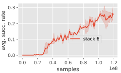
Figure 13: Average success rate of phasic-DT in “stack-6-cube” domain.

B.3 Algorithm Implementations

Network architecture: We use separate policy and value networks with the same architecture for PPO-based algorithms. The specific network architectures for different domains are as follows. For “Push”, we use MLPs of hidden size 400 and 300. For “Ant Maze”, the networks are MLPs of hidden size 256 and 256. For “Stacking”, we use a transformer (Vaswani et al., 2017)-based architecture, which stacks 2 self-attention blocks with one head and 64 hidden units, and then goes though linear heads to output action distributions or values. Since there are exponential number of possible actions as we discretize each action dimension into several bins, we assume different action dimensions are independent, and use separate linear heads to predict distributions of different dimensions.

PAIR implementation: We use PPO (Schulman et al., 2017) for online training and advantage weighted imitation learning for offline training by default. For PPO training, we use $N_{\textrm{worker}}$ parallel workers to collect transitions $(s,a,r,s^{\prime})$ from the environments synchronously. When applying the value-difference-based intrinsic reward, $r$ is replaced by the sum of environment reward and the intrinsic reward calculated with the current value network. After each worker gets $N_{\textrm{steps}}$ data points, we run $N_{\textrm{epoch}}$ epochs of PPO training by splitting all the collected on-policy data into $N_{\textrm{batch}}$ batches. The successful trajectories from these on-policy batch are directly stored into the offline data $\mathcal{D}$, and the failed trajectories are cached into a failure buffer $\mathcal{B}_{\textrm{fail}}$. We repeat the data collection - PPO training phase until the total amount of on-policy data reaches $N_{\textrm{online}}$. Then we perform data augmentation (task reduction, goal relabeling) over $\mathcal{B}_{\textrm{fail}}$ so as to generate more successful data, and insert the resulting demonstrations into $\mathcal{D}$ as well. After the dataset $\mathcal{D}$ is constructed, we run $M_{\textrm{epoch}}$ epochs of advantage weighted behavior cloning with batch size $m$. We use GAE advantage calculated with the value network learned after the online phase as $(R-V)$ for each data point. We use Adam optimizer (Kingma & Ba, 2015) for PPO and supervised learning. All the hyper-parameters are listed in Table 1.

We do not additionally train the value network using the offline dataset in offline phase since we empirically find that training $V$ does not help the overall performance (see Figure 14).

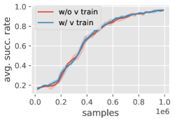
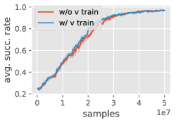
Figure 14: Comparison of training value network or not in PAIR offline phase. Left plot is in “Push” domain, right plot is in “Ant Maze”.

Domain	Push	Ant Maze	Stacking
$N_{\textrm{worker}}$	4	64	64
$N_{\textrm{online}}$	$10\cdot 2^{14}$	$20\cdot 2^{18}$	adaptive
$\alpha$	0.5
$N_{\textrm{steps}}$	4096
$N_{\textrm{epoch}}$	10
$N_{\textrm{batch}}$	32
$\beta$	1
$M_{\textrm{epoch}}$	10
$m$	64
lr	2.5e-4

Table 1: Hyperparameters of PAIR.

GCSL baseline implementation: There is a slight difference between our implementation and the original version from (Ghosh et al., 2020): we collect and relabel data in a more phasic fashion, i.e., we perform imitation learning on the data batch collected from only the previous online collection phase. We keep the number of online steps before offline imitation learning the same as PAIR. The original GCSL maintains a data buffer throughout the training process similar to the setting in off-policy RL. We find our phasic GCSL can get better performance than the original version (see Figure 16), so we present the results of phasic GCSL in the main paper.

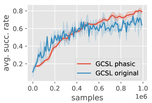
Figure 15: Comparison between phasic GCSL and the original version.

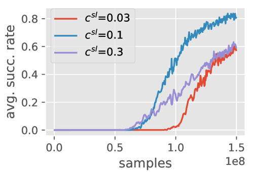
Figure 16: Success rate of joint RL+SL with different $c^{SL}$ in “stack-6-cube” task. We adopt $c^{SL}$ = 0.1 for SIR in the main paper.

DT baseline implementation: The policy and value networks adopt the same GPT-2 architecture similar to the original version in (Chen et al., 2021). They output actions and values conditioning on desired return, past states, and past actions. To avoid gradient explosion, only the last token of the predicted action or value sequence is used for updating the model. To stabilize training, we remove all dropout layers from the transformer model. We use a context length of 5 for sequence conditioning. The specific feature extractors for processing single-step observations in different domains are as follows. For “Push”, we use MLPs of hidden size 300 and 300 for representation learning and we train separate policy and value networks. For “Stacking”, we use a transformer-based architecture similar to PAIR for representation learning except that the size of hidden layer is 128. We find that using shared or separate feature extractors for policy and value networks leads to similar performances. Therefore we share parameters for them to save computational resources.

B.4 Analysis on Phasic vs. Joint RL and SL Optimization

PAIR decouples RL and SL objectives in two phases instead of optimizing them jointly ($L^{RL}+c^{SL}L^{SL}$), since the two objectives can largely interfere with each other and the choice of $c^{SL}$ is empirically brittle to tune. The RL objective is policy gradient over rollout data (Eqn. 1), which requires (primarily) on-policy samples (both success and failures) to make policy improvement. The SL objective (Eqn. 2) is performed over the successful dataset with both success-only rollout samples and off-policy augmentation trajectories. These two objectives operate on very distinct data distributions. If $c^{SL}$ is too large, the gradient will be pulled away from the policy improvement direction, which makes policy learning unstable or even breaks training. If $c^{SL}$ is too small, the objective may not sufficiently leverage the augmented successful data learning to slow convergence. We report sensitivity analysis in Fig. 16 by trying different $c^{SL}$ in the joint objective. With phasic training, RL and SL are decoupled and the interference is largely reduced. We can also intuitively interpret the benefit of decoupling RL and SL into two phases by echoing one result in stochastic optimization: smaller optimization step size should be taken when the gradient noise is large (Theorem 6.2 in  (Bubeck, 2015)). RL objective is with large gradient noise, while SL offers clear supervision signal. When jointly optimizing RL and SL, only small step size is allowed which leads to slow convergence; when optimizing RL and SL separately, different step sizes can be chosen for different objectives, thus converges faster.

References

- Akkaya et al. (2019) Akkaya, I., Andrychowicz, M., Chociej, M., Litwin, M., McGrew, B., Petron, A., Paino, A., Plappert, M., Powell, G., Ribas, R., et al. Solving rubik’s cube with a robot hand. arXiv preprint arXiv:1910.07113, 2019.
- Andrychowicz et al. (2017) Andrychowicz, M., Wolski, F., Ray, A., Schneider, J., Fong, R., Welinder, P., McGrew, B., Tobin, J., Abbeel, P., and Zaremba, W. Hindsight experience replay. In Proceedings of the 31st International Conference on Neural Information Processing Systems, pp. 5055–5065, 2017.
- Andrychowicz et al. (2021) Andrychowicz, M., Raichuk, A., Stańczyk, P., Orsini, M., Girgin, S., Marinier, R., Hussenot, L., Geist, M., Pietquin, O., Michalski, M., Gelly, S., and Bachem, O. What matters for on-policy deep actor-critic methods? a large-scale study. In International Conference on Learning Representations, 2021.
- Azuma (1967) Azuma, K. Weighted sums of certain dependent random variables. Tohoku Mathematical Journal, Second Series, 19(3):357–367, 1967.
- Bacon et al. (2017) Bacon, P.-L., Harb, J., and Precup, D. The option-critic architecture. In Proceedings of the Thirty-First AAAI Conference on Artificial Intelligence, pp. 1726–1734, 2017.
- Badia et al. (2020) Badia, A. P., Sprechmann, P., Vitvitskyi, A., Guo, D., Piot, B., Kapturowski, S., Tieleman, O., Arjovsky, M., Pritzel, A., Bolt, A., and Blundell, C. Never give up: Learning directed exploration strategies. In International Conference on Learning Representations, 2020. URL https://openreview.net/forum?id=Sye57xStvB.
- Brown et al. (2020) Brown, T., Mann, B., Ryder, N., Subbiah, M., Kaplan, J. D., Dhariwal, P., Neelakantan, A., Shyam, P., Sastry, G., Askell, A., Agarwal, S., Herbert-Voss, A., Krueger, G., Henighan, T., Child, R., Ramesh, A., Ziegler, D., Wu, J., Winter, C., Hesse, C., Chen, M., Sigler, E., Litwin, M., Gray, S., Chess, B., Clark, J., Berner, C., McCandlish, S., Radford, A., Sutskever, I., and Amodei, D. Language models are few-shot learners. In Larochelle, H., Ranzato, M., Hadsell, R., Balcan, M. F., and Lin, H. (eds.), Advances in Neural Information Processing Systems, volume 33, pp. 1877–1901. Curran Associates, Inc., 2020.
- Bubeck (2015) Bubeck, S. Convex optimization: Algorithms and complexity. Found. Trends Mach. Learn., 8(3-4):231–357, 2015. doi: 10.1561/2200000050.
- Burda et al. (2019) Burda, Y., Edwards, H., Storkey, A., and Klimov, O. Exploration by random network distillation. In International Conference on Learning Representations, 2019. URL https://openreview.net/forum?id=H1lJJnR5Ym.
- Chen et al. (2021) Chen, L., Lu, K., Rajeswaran, A., Lee, K., Grover, A., Laskin, M., Abbeel, P., Srinivas, A., and Mordatch, I. Decision transformer: Reinforcement learning via sequence modeling. arXiv preprint arXiv:2106.01345, 2021.
- Cobbe et al. (2021) Cobbe, K., Hilton, J., Klimov, O., and Schulman, J. Phasic policy gradient. In Meila, M. and Zhang, T. (eds.), Proceedings of the 38th International Conference on Machine Learning, ICML 2021, 18-24 July 2021, Virtual Event, volume 139 of Proceedings of Machine Learning Research, pp. 2020–2027. PMLR, 2021.
- Coumans & Bai (2016) Coumans, E. and Bai, Y. Pybullet, a python module for physics simulation for games, robotics and machine learning. 2016.
- Dosovitskiy et al. (2020) Dosovitskiy, A., Beyer, L., Kolesnikov, A., Weissenborn, D., Zhai, X., Unterthiner, T., Dehghani, M., Minderer, M., Heigold, G., Gelly, S., et al. An image is worth 16x16 words: Transformers for image recognition at scale. In International Conference on Learning Representations, 2020.
- Ecoffet et al. (2021) Ecoffet, A., Huizinga, J., Lehman, J., Stanley, K. O., and Clune, J. First return, then explore. Nature, 590(7847):580–586, 2021.
- Emmons et al. (2021) Emmons, S., Eysenbach, B., Kostrikov, I., and Levine, S. Rvs: What is essential for offline rl via supervised learning? arXiv preprint arXiv:2112.10751, 2021.
- Engstrom et al. (2020) Engstrom, L., Ilyas, A., Santurkar, S., Tsipras, D., Janoos, F., Rudolph, L., and Madry, A. Implementation matters in deep rl: A case study on ppo and trpo. In International Conference on Learning Representations, 2020.
- Eysenbach et al. (2020) Eysenbach, B., Salakhutdinov, R., and Levine, S. C-learning: Learning to achieve goals via recursive classification. In International Conference on Learning Representations, 2020.
- Fujimoto & Gu (2021) Fujimoto, S. and Gu, S. S. A minimalist approach to offline reinforcement learning. arXiv preprint arXiv:2106.06860, 2021.
- Furuta et al. (2021) Furuta, H., Matsuo, Y., and Gu, S. S. Generalized decision transformer for offline hindsight information matching. In Deep RL Workshop NeurIPS 2021, 2021.
- Ghosh et al. (2020) Ghosh, D., Gupta, A., Reddy, A., Fu, J., Devin, C. M., Eysenbach, B., and Levine, S. Learning to reach goals via iterated supervised learning. In International Conference on Learning Representations, 2020.
- Hester et al. (2018) Hester, T., Vecerik, M., Pietquin, O., Lanctot, M., Schaul, T., Piot, B., Horgan, D., Quan, J., Sendonaris, A., Osband, I., et al. Deep q-learning from demonstrations. In Thirty-second AAAI conference on artificial intelligence, 2018.
- Hwangbo et al. (2019) Hwangbo, J., Lee, J., Dosovitskiy, A., Bellicoso, D., Tsounis, V., Koltun, V., and Hutter, M. Learning agile and dynamic motor skills for legged robots. Science Robotics, 4(26), 2019.
- Ilyas et al. (2020) Ilyas, A., Engstrom, L., Santurkar, S., Tsipras, D., Janoos, F., Rudolph, L., and Madry, A. A closer look at deep policy gradients. In International Conference on Learning Representations, 2020.
- Janner et al. (2021) Janner, M., Li, Q., and Levine, S. Offline reinforcement learning as one big sequence modeling problem. Advances in Neural Information Processing Systems, 34, 2021.
- Jeon & Kim (2020) Jeon, W. and Kim, D. Autonomous molecule generation using reinforcement learning and docking to develop potential novel inhibitors. Scientific reports, 10(1):1–11, 2020.
- Jumper et al. (2021) Jumper, J., Evans, R., Pritzel, A., Green, T., Figurnov, M., Ronneberger, O., Tunyasuvunakool, K., Bates, R., Žídek, A., Potapenko, A., et al. Highly accurate protein structure prediction with alphafold. Nature, 596(7873):583–589, 2021.
- Kaelbling (1993) Kaelbling, L. Learning to achieve goals. In Proc. of IJCAI-93, pp. 1094–1098, 1993.
- Kidambi et al. (2020) Kidambi, R., Rajeswaran, A., Netrapalli, P., and Joachims, T. Morel: Model-based offline reinforcement learning. In NeurIPS, 2020.
- Kingma & Ba (2015) Kingma, D. P. and Ba, J. Adam: A method for stochastic optimization. In ICLR (Poster), 2015.
- Kostrikov et al. (2021) Kostrikov, I., Nair, A., and Levine, S. Offline reinforcement learning with implicit q-learning. arXiv preprint arXiv:2110.06169, 2021.
- Kulkarni et al. (2016) Kulkarni, T. D., Narasimhan, K., Saeedi, A., and Tenenbaum, J. Hierarchical deep reinforcement learning: Integrating temporal abstraction and intrinsic motivation. Advances in neural information processing systems, 29:3675–3683, 2016.
- Kumar et al. (2019) Kumar, A., Peng, X. B., and Levine, S. Reward-conditioned policies. arXiv preprint arXiv:1912.13465, 2019.
- Kumar et al. (2020) Kumar, A., Zhou, A., Tucker, G., and Levine, S. Conservative q-learning for offline reinforcement learning. In Larochelle, H., Ranzato, M., Hadsell, R., Balcan, M., and Lin, H. (eds.), Advances in Neural Information Processing Systems 33: Annual Conference on Neural Information Processing Systems 2020, NeurIPS 2020, December 6-12, 2020, virtual, 2020.
- Lange et al. (2012) Lange, S., Gabel, T., and Riedmiller, M. Batch reinforcement learning. In Reinforcement learning, pp. 45–73. Springer, 2012.
- Levine (2021) Levine, S. Understanding the world through action. In Faust, A., Hsu, D., and Neumann, G. (eds.), Conference on Robot Learning, 8-11 November 2021, London, UK, volume 164 of Proceedings of Machine Learning Research, pp. 1752–1757. PMLR, 2021.
- Levine et al. (2020) Levine, S., Kumar, A., Tucker, G., and Fu, J. Offline reinforcement learning: Tutorial, review, and perspectives on open problems. arXiv preprint arXiv:2005.01643, 2020.
- Li et al. (2020a) Li, R., Jabri, A., Darrell, T., and Agrawal, P. Towards practical multi-object manipulation using relational reinforcement learning. In 2020 IEEE International Conference on Robotics and Automation (ICRA), pp. 4051–4058. IEEE, 2020a.
- Li et al. (2020b) Li, Y., Wu, Y., Xu, H., Wang, X., and Wu, Y. Solving compositional reinforcement learning problems via task reduction. In International Conference on Learning Representations, 2020b.
- Lillicrap et al. (2016) Lillicrap, T. P., Hunt, J. J., Pritzel, A., Heess, N., Erez, T., Tassa, Y., Silver, D., and Wierstra, D. Continuous control with deep reinforcement learning. In ICLR (Poster), 2016.
- Lu et al. (2021) Lu, Y., Hausman, K., Chebotar, Y., Yan, M., Jang, E., Herzog, A., Xiao, T., Irpan, A., Khansari, M., Kalashnikov, D., and Levine, S. AW-opt: Learning robotic skills with imitation andreinforcement at scale. In 5th Annual Conference on Robot Learning, 2021. URL https://openreview.net/forum?id=xwEaXgFa0MR.
- Lynch et al. (2020) Lynch, C., Khansari, M., Xiao, T., Kumar, V., Tompson, J., Levine, S., and Sermanet, P. Learning latent plans from play. In Conference on Robot Learning, pp. 1113–1132. PMLR, 2020.
- Mao et al. (2022) Mao, Y., Wang, C., Wang, B., and Zhang, C. Moore: Model-based offline-to-online reinforcement learning, 2022.
- Matsushima et al. (2020) Matsushima, T., Furuta, H., Matsuo, Y., Nachum, O., and Gu, S. Deployment-efficient reinforcement learning via model-based offline optimization. In International Conference on Learning Representations, 2020.
- Mnih et al. (2015) Mnih, V., Kavukcuoglu, K., Silver, D., Rusu, A. A., Veness, J., Bellemare, M. G., Graves, A., Riedmiller, M., Fidjeland, A. K., Ostrovski, G., et al. Human-level control through deep reinforcement learning. nature, 518(7540):529–533, 2015.
- Nachum et al. (2018) Nachum, O., Gu, S. S., Lee, H., and Levine, S. Data-efficient hierarchical reinforcement learning. Advances in Neural Information Processing Systems, 31:3303–3313, 2018.
- Nair et al. (2018a) Nair, A., McGrew, B., Andrychowicz, M., Zaremba, W., and Abbeel, P. Overcoming exploration in reinforcement learning with demonstrations. In 2018 IEEE International Conference on Robotics and Automation (ICRA), pp. 6292–6299. IEEE, 2018a.
- Nair et al. (2020) Nair, A., Dalal, M., Gupta, A., and Levine, S. Awac: Accelerating online reinforcement learning with offline datasets. 2020.
- Nair et al. (2018b) Nair, A. V., Pong, V., Dalal, M., Bahl, S., Lin, S., and Levine, S. Visual reinforcement learning with imagined goals. Advances in Neural Information Processing Systems, 31:9191–9200, 2018b.
- Nasiriany et al. (2019) Nasiriany, S., Pong, V., Lin, S., and Levine, S. Planning with goal-conditioned policies. Advances in Neural Information Processing Systems, 32:14843–14854, 2019.
- Oh et al. (2018) Oh, J., Guo, Y., Singh, S., and Lee, H. Self-imitation learning. In International Conference on Machine Learning, pp. 3878–3887. PMLR, 2018.
- Peng et al. (2019) Peng, X. B., Kumar, A., Zhang, G., and Levine, S. Advantage-weighted regression: Simple and scalable off-policy reinforcement learning. arXiv preprint arXiv:1910.00177, 2019.
- Pong et al. (2018) Pong, V., Gu, S., Dalal, M., and Levine, S. Temporal difference models: Model-free deep rl for model-based control. In International Conference on Learning Representations, 2018.
- Rajeswaran et al. (2018) Rajeswaran, A., Kumar, V., Gupta, A., Vezzani, G., Schulman, J., Todorov, E., and Levine, S. Learning complex dexterous manipulation with deep reinforcement learning and demonstrations. In Kress-Gazit, H., Srinivasa, S. S., Howard, T., and Atanasov, N. (eds.), Robotics: Science and Systems XIV, Carnegie Mellon University, Pittsburgh, Pennsylvania, USA, June 26-30, 2018, 2018. doi: 10.15607/RSS.2018.XIV.049. URL http://www.roboticsproceedings.org/rss14/p49.html.
- Rashidinejad et al. (2021) Rashidinejad, P., Zhu, B., Ma, C., Jiao, J., and Russell, S. Bridging offline reinforcement learning and imitation learning: A tale of pessimism. arXiv preprint arXiv:2103.12021, 2021.
- Schaul et al. (2015) Schaul, T., Horgan, D., Gregor, K., and Silver, D. Universal value function approximators. In International conference on machine learning, pp. 1312–1320. PMLR, 2015.
- Schmidhuber (2019) Schmidhuber, J. Reinforcement learning upside down: Don’t predict rewards–just map them to actions. arXiv preprint arXiv:1912.02875, 2019.
- Schrittwieser et al. (2020) Schrittwieser, J., Antonoglou, I., Hubert, T., Simonyan, K., Sifre, L., Schmitt, S., Guez, A., Lockhart, E., Hassabis, D., Graepel, T., et al. Mastering atari, go, chess and shogi by planning with a learned model. Nature, 588(7839):604–609, 2020.
- Schulman et al. (2017) Schulman, J., Wolski, F., Dhariwal, P., Radford, A., and Klimov, O. Proximal policy optimization algorithms. CoRR, abs/1707.06347, 2017. URL http://arxiv.org/abs/1707.06347.
- Singh et al. (2005) Singh, S., Barto, A. G., and Chentanez, N. Intrinsically motivated reinforcement learning. Technical report, MASSACHUSETTS UNIV AMHERST DEPT OF COMPUTER SCIENCE, 2005.
- Stolle & Precup (2002) Stolle, M. and Precup, D. Learning options in reinforcement learning. In International Symposium on abstraction, reformulation, and approximation, pp. 212–223. Springer, 2002.
- Todorov et al. (2012) Todorov, E., Erez, T., and Tassa, Y. Mujoco: A physics engine for model-based control. In 2012 IEEE/RSJ International Conference on Intelligent Robots and Systems, pp. 5026–5033. IEEE, 2012.
- Tucker et al. (2018) Tucker, G., Bhupatiraju, S., Gu, S., Turner, R., Ghahramani, Z., and Levine, S. The mirage of action-dependent baselines in reinforcement learning. In International conference on machine learning, pp. 5015–5024. PMLR, 2018.
- Uchendu et al. (2022) Uchendu, I., Xiao, T., Lu, Y., Zhu, B., Yan, M., Simon, J., Bennice, M., Fu, C., Ma, C., Jiao, J., et al. Jump-start reinforcement learning. arXiv preprint arXiv:2204.02372, 2022.
- Vaswani et al. (2017) Vaswani, A., Shazeer, N., Parmar, N., Uszkoreit, J., Jones, L., Gomez, A. N., Kaiser, Ł., and Polosukhin, I. Attention is all you need. In Advances in neural information processing systems, pp. 5998–6008, 2017.
- Veeriah et al. (2018) Veeriah, V., Oh, J., and Singh, S. Many-goals reinforcement learning. arXiv preprint arXiv:1806.09605, 2018.
- Wu et al. (2019) Wu, Y., Tucker, G., and Nachum, O. Behavior regularized offline reinforcement learning. arXiv preprint arXiv:1911.11361, 2019.
- Yu et al. (2021a) Yu, C., Velu, A., Vinitsky, E., Wang, Y., Bayen, A., and Wu, Y. The surprising effectiveness of mappo in cooperative, multi-agent games. arXiv preprint arXiv:2103.01955, 2021a.
- Yu et al. (2021b) Yu, T., Kumar, A., Chebotar, Y., Hausman, K., Levine, S., and Finn, C. Conservative data sharing for multi-task offline reinforcement learning. Advances in Neural Information Processing Systems, 34, 2021b.
- Zhao et al. (2019) Zhao, R., Sun, X., and Tresp, V. Maximum entropy-regularized multi-goal reinforcement learning. In International Conference on Machine Learning, pp. 7553–7562. PMLR, 2019.