Exploring the transition from BCS to unitarity without Cooper pairs: the Pauli principle, normal modes and superfluidity.

Abstract

The transition from the weakly interacting BCS regime to the strongly interacting unitary regime is explored for ultracold trapped Fermi gases assuming a normal mode description of the gas instead of the conventional Cooper pairing. The Pauli principle is applied “on paper” by using specific normal mode assignments. Energies, entropies, critical temperatures, and an excitation frequency are studied and compared to existing results in the literature. These normal modes have been derived analytically for $N$ identical, confined particles from a first-order $L=0$ group theoretic solution of a three-dimensional Hamiltonian with a general two-body interaction. In previous studies, normal modes were able to describe the unitary regime obtaining ground state energies comparable to benchmark results and thermodynamics quantities in excellent agreement with experiment. In a recent study, the behavior of the normal mode frequencies was investigated for Hamiltonians with a range of interparticle interaction strengths from BCS to unitarity in the first test of this approach beyond the unitary regime, and a microscopic basis of the large excitation gaps and universal behavior at unitarity was proposed. Based on the success of these earlier studies, the current paper continues to explore the ability of normal modes to describe superfluidity along the BCS to unitarity transition. The results confirm earlier conclusions that the physics of superfluidity can be described using normal modes across a wide range of interparticle interaction strengths and offers an alternative to the two-body pairing models commonly used to describe superfluidity along this transition.

I Introduction

The BCS to unitarity transition for ultracold gaseous fermions has been investigated both experimentally and theoretically since this transition was first achieved in the laboratoryjin1 ; jin2 ; zwierlein1 ; zwierlein2 ; grimm1 ; salomon1 ; thomas1 ; hulet1 ; jochim1 . Theoretical methods typically assume that the atomic fermions are forming Cooper pairs to explain the emergence of superfluid behaviorgiorgini1 ; randeria1 ; leggett1 ; leggett2 ; bcs ; eagles ; nozieres . When a Feshbach resonance is tuned to weak interactions, the neutral atoms bind into loosely-bound pairs whose size decreases as the interparticle interaction strength increases toward the unitarity. Eventually diatomic molecules are produced that condense in the BEC regime. In materials that support superconductivity, the binding of electrons into Cooper pairs at long distances is thought to be mediated by phonon interactions in the underlying material producing a weak attractionbcs ; leggett1 ; leggett2 ; eagles ; nozieres .

In a series of recent papers, the ability of normal modes to describe superfluidity has been investigated for ultracold Fermi gasesprl ; emergence ; prafreq . Initial studies were in the unitary regime where results for ground state energies comparable to benchmark resultsprl and thermodynamic quantities in excellent agreement with experiment were obtainedemergence . The $N$-body analytic frequencies of the normal modes were studied from the BCS regime to unitarityprafreq revealing the emergence of excitation gaps that increased from extremely small gaps deep in the BCS regime to a maximum at unitarity as observed in experiments. The microscopic dynamics responsible for the emergence of these gaps was investigated using the analytic forms of the normal mode functions and a microscopic basis for the universal behavior at unitarity was proposed. These calculations have modest numerical requirements since the $N$-body normal modes have been derived in analytic form using group theoretic techniquespaperI ; JMPpaper .

In this paper, I continue to explore the ability of normal modes to describe superfluidity from BCS to unitarity by determining various properties along this transition including ground state energies, thermodynamic entropies, critical temperatures, and the breathing excitation frequency, comparing to both experiment and theory. This approach models the physics by assuming many-body pairing exhibited through normal modes, i.e. coherent, collisionless motion of the fermions that minimizes interparticle interactions and makes two-body pairing irrelevant since it is impossible to discern which fermion is paired with another fermion.

Normal mode functions naturally provide simple, coherent macroscopic wave functions that maintain phase coherence over the entire ensemble, and give rise to “quasiparticles” defined by the excitations between the modes. At ultracold temperatures, only the lowest two types of normal mode frequencies are relevant, gapless phonon modes with very low frequencies and particle-hole excitation modes.

Normal mode motions exist at all scales in our universe from vibrating crystalsNM4 to oscillating black holesNM10 . The particles in a normal mode move in synchrony with the same frequency and phase, allowing a description of the complex, simultaneous motions of many interacting particles in terms of collective behavior. These modes are a manifestation of the widespread appearance of vibrational motions that occur in nature in diverse media and across many orders of magnitudeNM1 ; NM2 ; NM3 ; NM4 ; NM5 ; NM6 ; NM7 ; NM8 ; NM9 ; NM10 ; NM11 ; NM12 ; NM13 . When higher order effects are small, vibrational behavior couples into stable collective motion, thus incorporating the many-body effects of large ensembles into simple dynamic motions. These collective motions correspond to the eigenfunctions of an approximate Hamiltonian and thus will possess some stability over time. Normal modes will reflect the symmetry that is present in this approximate Hamiltonian and can offer beyond-mean-field analytic many-body solutions and physical intuition into the microscopic dynamics responsible for diverse phenomena.

SPT formalism.

The formalism used to obtain these normal modes is called symmetry-invariant perturbation theory (SPT), a first-principle, non-numerical method which use group theoretic and graphical techniques to solve many-body problems. This perturbation formalism was initially developed for bosonsFGpaper ; energy ; paperI ; JMPpaper ; laingdensity ; test ; toth and has been formulated through first order for $L=0$, three-dimensional systems with completely general interaction potentials and spherically-symmetric confining potentials. Unlike conventional methods for which the resources for an exact solution of the quantum $N$-body wave function scale exponentially with $N$, typically doubling for every particle addedliu ; montina2008 , the SPT approach employs symmetry to attack the $N$-scaling problemtest . This is accomplished by formulating a perturbation series about a large-dimension configuration whose point group is isomorphic to the symmetric group $S_{N}$ , and then evaluating the series for $D=3$. Group theoretic techniques are used to extract the part of the problem that scales exponentially with complexity as a pure mathematical problem (cf. the Wigner-Eckart theorem), which can then be solved as a function of $N$, rendering the interaction dynamics containing the “physics” independent of $N$rearrangeprl ; complexity . The perturbation terms are evaluated for large dimension where the structure has maximum symmetry yielding terms that are invariant under the $N!$ operations of the $S_{N}$ point group. This strategy produces a problem at each order that, in principle, can be solved exactly, analytically using symmetry. Although extremely challenging, the mathematical work at each order can be saved and used to study a problem with a new interaction potential significantly reducing numerical demands.

The symmetry constraints are enforced by using a tensor basis that is small, complete and $S_{N}$-invariant. (A proof of the completeness is in Ref test .) As $N$ increases, the $N!$ operations of $S_{N}$ place increasing constraints on the basis whose size, therefore, does not grow with $N$. First order needs only seven elements while the next order requires twenty-five elements regardless of the $N$ value. (See Section  II.3.) These tensor basis functions are called “binary invariants” reflecting their invariance under the symmetric group operations and the use of $1^{\prime}s$ and $0^{\prime}s$ in their tensor definition. When this basis is used for the perturbation expansion, the Hamiltonian will automatically be invariant at each order.

The SPT formalism accounts for every two-particle interaction rather than assuming an average interaction and can be applied to strongly interacting systems since the perturbation is not dependent on the interaction. Even at the lowest perturbation order, the SPT method includes beyond-mean-field effects underlying the excellent results achieved at first order using this SPT methodenergy ; prl ; emergence as well as earlier dimensional approachesherschbach1 ; herschbach2 ; loeser ; kais1 ; kais2 .

This formalism has also been implemented for a model problem of harmonically-confined, harmonically-interacting particles that is exactly solvabletest ; toth ; harmoniumpra ; partition . Agreement to ten or more digits of accuracy was found for the wave function compared to the exact wave function obtained independently, verifying this general many-body formalism for a three-dimensional, many-body system that is fully-interacting test including the formulas derived analytically for the $N$-body normal mode coordinates and frequencies.

Application to fermions.

The application of SPT to fermions has been developed in the last seven yearsprl ; harmoniumpra ; partition ; emergence ; annphys ; prafreq . Initially, these studies focused on the unitary regime where I obtained excellent values for the ground state energies comparable to numerically intensive benchmark methodsprl as well as thermodynamic quantities for the energy, entropy, and specific heat in close agreement with experimentemergence . The lambda transition in the specific heat was clearly seen defining a critical temperature for the onset of superfluidity in the unitary regime. These results support the validity of this normal mode description of superfluidity and the role of the Pauli principle in low temperature dynamicsemergence . The heavy numerical demands of enforcing antisymmetry in fermion systems in conventional theoretical approaches is avoided in the SPT approach by enforcing the Pauli principle “on paper” using specific occupations of the normal modes at first orderprl ; harmoniumpra ; emergence ; partition . (See Section II.5.) Beyond-mean-field groundprl and excited stateemergence energies and their degeneracies have been calculated enabling the determination of a partition function and the calculation of thermodynamic quantitiespartition ; emergence . An accurate partition function requires many states chosen from the infinite spectrum by the Pauli principle, thus relating the Pauli principle to many-body interaction dynamics through the normal modes.

The physical character of the normal modes.

The close agreement with experiment for energies and thermodynamic observables in the unitary regime motivated an investigation into the physical character of the normal modes with the goal of obtaining insight into the dynamics of cooperative motionannphys and the universal behavior at unitarity. In a recent paper, I used the analytic $N$-body normal mode coordinates to study the character of the five types of normal modesannphys , investigating their evolving motions as a function of $N$, from small $N$ to large ensembles. I analyzed the contributions of the particles individually to the collective motion, making some general observations based on symmetry considerations, and then focusing on the unitary Hamiltonian.

This study found a smooth evolution as $N$ increases from the expected behavior for few-body systems whose motions are analogous to those of molecular equivalents such as ammonia and methane, to the coherent motions observed in large $N$ ensembles. Furthermore, the transition from few-body to large $N$ behavior happens at surprisingly low values of $N$ ($N\approx 10$) validating the results of numerous few-body studiesadhikari ; hu6 ; hu7 ; hu8 ; blume1 ; blume2 ; levinsen ; grining . This evolution in character from few-body to large ensembles is dictated by rather simple analytic forms (See Ref. emergence after Eq. (31).) that nevertheless take into account the complicated interplay of the particles as they interact and cooperate to create coherent macroscopic motion. This evolution of behavior was dependent primarily on the symmetry present in the Hamiltonian, and thus could be relevant for diverse phenomena at different scales if the same symmetry exists or is dominant. Also, two phenomena were found that could support the emergence and stabilization of collective behavior for the unitary regime.

The evolution of the normal mode frequencies.

In my most recent study, I extended my investigation beyond unitarity, studying the evolution of the analytic frequencies as a function of the interparticle interaction strength, $\bar{V}_{\mathtt{int}}\sim\bar{V}_{0}$, (See Eq. (8).) for fixed ensemble sizes from BCS to unitarityprafreq . I focused on larger values of $N$ relevant to laboratory studies of this transition that use a Feshbach resonance to tune the interaction. This work offers insight into the microscopic behavior leading to large gaps and universal behavior at unitarity and offers the possibility of controlling the appearance and stability of excitation gaps by fine tuning system parameters.

This analysis revealed the appearance of excitation gaps that increase as $\bar{V}_{0}$ increases. At the independent particle limit where interactions vanish, all five frequencies limit to the same value at twice the trap frequency. As $\bar{V}_{0}$ turns on, the frequencies slowly spread out producing gaps that are maximal at unitarity.

The microscopic dynamics underpinning universal behavior.

The microscopic dynamics underpinning the emergence of universal behavior at unitarity and the convergence of the angular frequencies to integer multiples of the trap frequency were investigated using two approaches. First, the effect of different Hamiltonian terms on the analytic frequencies was tracked as $\bar{V}_{0}$ changes. Second, the motion of each particle in the normal mode coordinate was analyzed to discern how the ensemble rearranges microscopically as interactions begin and cooperative behavior emerges. At unitarity, the angular particle-hole frequency converges to the frequency of the trap and sets up an evenly-spaced spectrum identical to the independent particle spectrum. Also, as $\bar{V}_{0}$ increases, correlation of the particles increases minimizing the interparticle interactions. These results are consistent with the universal behavior expected at unitarity and offer insight into its microscopic basis.

The study of the frequencies across the BCS to unitarity transition suggested that normal modes are able to describe the physics of ultracold Fermi gases including superfluidity for a range of interaction strengths and to offer insight into the underlying microscopic basis without the assumption of two-body pairing. In the current paper, I now look more closely at the ability of these first-order normal mode solutions to accurately describe the BCS to unitarity transition by determining various properties along this transition. The value of $\bar{V}_{0}$ is scaled so $\bar{V}_{0}=1.0$ in the unitary regime, while the BCS region is loosely-defined by very weak interparticle interactions, e.g. $\bar{V}_{0}\approx 10^{-6}$. This potential is defined in Section II with a more detailed description in Appendix A in Ref. annphys .

II The General N-body problem: A Group Theoretic and Graphical Approach

This section contains a summary of the SPT formalism including the symmetry coordinates, the normal modes and their frequencies presented in Refs. paperI ; FGpaper .

II.1 The Hamiltonian

For $N$ interacting particles, the Schrödinger equation in $D$ dimensions is:

$$H\Psi=\left[\sum\limits_{i=1}^{N}h_{i}+\sum_{i=1}^{N-1}\sum\limits_{j=i+1}^{N}g_{ij}\right]\Psi=E\Psi\,,$$ (1)

$$\begin{array}[]{rcl}h_{i}&=&-\frac{\hbar^{2}}{2m_{i}}\sum\limits_{\nu=1}^{D}\frac{\partial^{2}}{\partial x_{i\nu}^{2}}+V_{\mathtt{conf}}\left(\sqrt{\sum\nolimits_{\nu=1}^{D}x_{i\nu}^{2}}\right)\,,\\ g_{ij}&=&V_{\mathtt{int}}\left(\sqrt{\sum\nolimits_{\nu=1}^{D}\left(x_{i\nu}-x_{j\nu}\right)^{2}}\right),\end{array}$$ (2)

where $h_{i}$ is the single-particle Hamiltonian, $g_{ij}$ a two-body interaction potential, $x_{i\nu}$ the $\nu^{th}$ Cartesian component of the $i^{th}$ particle, and $V_{\mathtt{conf}}$ is a spherically-symmetric confining potentialpaperI ; FGpaper ; JMPpaper . Defining internal coordinates as the $D$-dimensional scalar radii $r_{i}$ of the $N$ particles from the center of the trap and the cosines $\gamma_{ij}$ of the $N(N-1)/2$ interparticle angles between the radial vectors:

$$\begin{array}[]{rcl}r_{i}&=&\sqrt{\sum_{\nu=1}^{D}x_{i\nu}^{2}}\,,\;\;\;(1\leq i\leq N)\,,\\ \gamma_{ij}&=&cos(\theta_{ij})=\left(\sum_{\nu=1}^{D}x_{i\nu}x_{j\nu}\right)/r_{i}r_{j}\,,\end{array}$$ (3)

$(1\leq i<j\leq N)$ , the Schrödinger equation is transformed from Cartesian to internal coordinates.

A similarity transformationavery removes the first-order derivatives, and a scale factor, $\kappa(D)=D^{2}\bar{a}_{ho}$, is used to regularize the large-dimension limit of the Schrödinger equation by defining dimensionally-scaled oscillator length units where $\bar{a}_{\mathtt{ho}}=\sqrt{\frac{\hbar}{m\bar{\omega}_{\mathtt{ho}}}}$ and ${\bar{\omega}_{\mathtt{ho}}}=D^{3}{\omega_{\mathtt{ho}}}$. Substituting the scaled variables, $\bar{r}_{i}=r_{i}/\kappa(D)$, with $\bar{E}=\frac{E}{\hbar\bar{\omega}_{\mathtt{ho}}}$ and $\bar{H}=\frac{H}{\hbar\bar{\omega}_{\mathtt{ho}}}$, into the similarity-transformed Schrödinger equation gives:

$$\bar{H}\Phi=\left(\delta^{2}\bar{T}+\bar{U}+\bar{V}_{\mathtt{conf}}+\bar{V}_{\mathtt{int}}\right)\Phi=\bar{E}\,\Phi\,.$$ (4)

where

$$\begin{split}\bar{T}&=\sum\limits_{i=1}^{N}\Bigl{(}-\frac{1}{2}\frac{\partial^{2}}{{\partial\bar{r}_{i}}^{2}}\\ &-\frac{1}{2\bar{r}_{i}^{2}}\sum\limits_{j\not=i}\sum\limits_{k\not=i}\frac{\partial}{\partial\gamma_{ij}}(\gamma_{jk}-\gamma_{ij}\gamma_{ik})\frac{\partial}{\partial\gamma_{ik}}\Bigr{)}\,,\end{split}$$ (5)

$$\bar{U} = \sum\limits_{i=1}^{N}\left(\frac{\delta^{2}N(N-2)+(1-\delta(N+1))^{2}\left(\frac{\Gamma^{(i)}}{\Gamma}\right)}{8\bar{r}_{i}^{2}}\right)\,,$$ (6)

$$\bar{V}_{\mathtt{conf}} = \sum\limits_{i=1}^{N}\frac{1}{2}\bar{r}_{i}^{2}$$ (7)

$$\bar{V}_{\mathtt{int}} = \frac{\bar{V}_{0}}{1-3b^{\prime}\delta}\sum\limits_{i=1}^{N-1}\sum\limits_{j=i+1}^{N}\left(1-\tanh\Theta_{i,j}\right)\,,\$$ (8)

and $\delta=1/D$, $\Gamma$ is the Gramian determinant which has elements $\gamma_{ij}$ (See Appendix D in Ref FGpaper .), $\Gamma^{(i)}$ the determinant which has the $i^{th}$ row and column deleted, and $\hbar=m=1$. The barred quantities are scaled by $\kappa(D)$.

The interaction potential, $\bar{V}_{\mathtt{int}}$, reduces to a square well for $D=3$. The value of the constant $b^{\prime}$ yields a scattering length of infinity when $\bar{V}_{0}=1.0$. $\bar{V}_{0}$ is scaled to smaller values to reach the weaker interactions of the BCS regime. The argument $\Theta_{ij}$ is:

$$\Theta_{ij}=\frac{\bar{c}_{0}}{1-3\delta}\left(\frac{\bar{r}_{ij}}{\sqrt{2}}-\bar{\alpha}-3\delta\left(\bar{R}-\bar{\alpha}\right)\right)\,,$$ (9)

where $\bar{r}_{ij}={\sqrt{{\bar{r}_{i}}^{2}+{\bar{r}_{j}}^{2}-2\bar{r}_{i}\bar{r}_{j}\gamma_{ij}}}\,$ is the interatomic separation, $\bar{R}$ is the dimensionally-scaled range of the square-well potential, and $\bar{\alpha}$ is a constant that softens the potential as $D\rightarrow\infty$. $R$ is chosen so $R<<a_{ho}$ ($a_{ho}=\sqrt{\hbar/(m\omega_{ho})}$) and is extrapolated to zero-range interaction.

At the $D\to\infty$ limit, the second derivative terms of the kinetic energy drop out resulting in a static zeroth-order problem with an effective potential, $\bar{V}_{\mathtt{eff}}$:

$$\bar{V}_{\mathtt{eff}}(\bar{r},\gamma;\delta) = \sum\limits_{i=1}^{N}\left(\bar{U}(\bar{r}_{i};\delta)+\bar{V}_{\mathtt{conf}}(\bar{r}_{i};\delta)\right)$$ (10)

$$+\sum\limits_{i=1}^{N-1}\sum\limits_{j=i+1}^{N}\bar{V}_{\mathtt{int}}(\bar{r}_{i},\gamma_{ij};\delta)\,.$$

The minimum of $\bar{V}_{\mathtt{eff}}$ corresponds to a large-dimension maximally-symmetric configuration that has all radii, $\bar{r}_{i}$, and angle cosines, $\gamma_{ij}$, of the particles equal, i.e. when $D\to\infty$, $\bar{r}_{i}=\bar{r}_{\infty}\;\;(1\leq i\leq N)$ and $\gamma_{ij}={\gamma}_{\infty}\;\;(1\leq i<j\leq N)$. These parameters are solved using two minimum conditions: $\left(\frac{\partial\bar{V}_{\text{eff}}}{\partial\bar{r}_{i}}\right)\Biggr{|}_{\infty}=0,\,\,\left(\frac{\partial\bar{V}_{\text{eff}}}{\partial\gamma_{ij}}\right)\Biggr{|}_{\infty}=0\,.$ Using the definition of $\bar{V}_{\textrm{eff}}$, two equations in $\bar{r}_{\infty}$ and $\gamma_{\infty}$ yield: $\bar{r}_{\infty}=\frac{1}{\sqrt{2}\sqrt{1+(N-1)\gamma_{\infty}}}\,,$ while $\gamma_{\infty}$ is solved using the transcendental equation:

$$\frac{\gamma_{\infty}\left(2+(N-2)\gamma_{\infty}\right)}{\left(1-\gamma_{\infty}\right){}^{3/2}\sqrt{1+(N-1)\gamma_{\infty}}}+\bar{V}_{0}\,\text{sech}^{2}\left(\Theta_{\infty}\right)\Theta_{\infty}^{\prime}=0\,.$$ (11)

In the large-$D$ limit ($\delta\rightarrow 0$), the argument $\Theta_{ij}$ becomes: $\Theta_{\infty}=\Theta_{ij}\Biggr{|}_{\infty}=\bar{c}_{0}\left(\sqrt{1-\gamma_{\infty}}\,\bar{r}_{\infty}-\bar{\alpha}\right)\,.$

II.2 The Dimensional Expansion

The energy minimum as $\delta\rightarrow 0$, $\bar{E}_{\infty}$, is the starting point for the $1/D$ expansion. The $N(N+1)/2$ internal coordinates, $\bar{r}_{i}$ and $\gamma_{ij}$, are expanded as: $\bar{r}_{i}=\bar{r}_{\infty}+\delta^{1/2}\bar{r}^{\prime}_{i}$ and $\gamma_{ij}={\gamma}_{\infty}+\delta^{1/2}{\gamma}^{\prime}_{ij}$ setting up a power series in $\delta^{1/2}$ about the $D\to\infty$ symmetric minimum. The primed variables, $\bar{r}^{\prime}_{i}$ and $\overline{\gamma}^{\prime}_{ij}$ , are dimensionally-scaled internal displacement coordinates: The expansions of the Hamiltonian, wave function, and energy in powers of $\delta^{1/2}$ are:

$$\begin{array}[]{r@{}l@{}c}{\displaystyle\bar{H}=\bar{H}_{\infty}+\delta^{\frac{1}{2}}\,\bar{H}_{-1}+\delta}&{\displaystyle\,\sum_{j=0}^{\infty}\left(\delta^{\frac{1}{2}}\right)^{j}\bar{H}_{j}}&\\ {\displaystyle\Phi(\bar{r}_{i},\gamma_{ij})=}&{\displaystyle\,\sum_{j=0}^{\infty}\left(\delta^{\frac{1}{2}}\right)^{j}\Phi_{j}}&\\ {\displaystyle\bar{E}=\bar{E}_{\infty}+\delta^{\frac{1}{2}}\,\bar{E}_{-1}+\delta}&{\displaystyle\,\sum_{j=0}^{\infty}\left(\delta^{\frac{1}{2}}\right)^{j}\bar{E}_{j}}&\,,\end{array}$$ (12)

where

$$\bar{H}_{\infty} = \bar{E}_{\infty}$$ (13)

$$\bar{H}_{-1} = \bar{E}_{2n-1}=0\,,$$ (14)

$$\bar{H}_{0} = -\frac{1}{2}\,{}^{(0)}_{\ 2}G_{\nu_{1},\nu_{2}}\,\partial_{{\bar{y}^{\prime}}_{\nu_{1}}}\partial_{{\bar{y}^{\prime}}_{\nu_{2}}}+\frac{1}{2}\,{}^{(0)}_{\ 2}F_{\nu_{1},\nu_{2}}\,\bar{y}^{\prime}_{\nu_{1}}\bar{y}^{\prime}_{\nu_{2}}$$ (15)

$$+\,{}^{(0)}_{\ 0}F\,\,,$$

$$\bar{H}_{1} = -\frac{1}{2}\,{}^{(1)}_{\ 3}G_{\nu_{1},\nu_{2},\nu_{3}}\,\bar{y}^{\prime}_{\nu_{1}}\partial_{{\bar{y}^{\prime}}_{\nu_{2}}}\partial_{{\bar{y}^{\prime}}_{\nu_{3}}}-\frac{1}{2}\,{}^{(1)}_{\ 1}G_{\nu}\,\partial_{{\bar{y}^{\prime}}_{\nu}}$$ (16)

$$+\frac{1}{3!}\,{}^{(1)}_{\ 3}F_{\nu_{1},\nu_{2},\nu_{3}}\,\bar{y}^{\prime}_{\nu_{1}}\bar{y}^{\prime}_{\nu_{2}}\bar{y}^{\prime}_{\nu_{3}}+\,{}^{(1)}_{\ 1}F_{\nu}\,\bar{y}^{\prime}_{\nu}\,.$$

The superprescript in parentheses on the $\bm{F}$ and $\bm{G}$ tensors in Eqs. (15)-(16) denotes the order in $\delta^{1/2}$ in the sum over $j$ in Eq. (12). The subprescripts give the rank, $R$, of the tensors. The $G$ elements are defined from the first-order derivative terms, ${\bar{T}}$, of the Hamiltonian while the $F$ elements contain the first-order potential terms from ${\bar{V}_{\mathtt{eff}}}$. Appendix B of Ref. energy gives formulas for the $F$ and $G$ elements.

II.3 The Binary Invariant Basis

A tensor basis of binary invariants is used to obtain the $N$-body perturbation solutions exactly through first orderJMPpaper ; test ; toth . A rank $R$ tensor has dimension $[N(N+1)/2]^{R}$ and is comprised of $[N(N+1)/2]^{R}$ elements, either 1’s or 0’s positioned so the tensor is invariant under the $N!$ operations of $S_{N}$. At each order, the binary invariants constitute a complete basis spanning the tensor space. Each binary invariant can be represented by an unlabelled multiloop graph (with no unattached vertices)epaps .

For example, irrespective of the value of $N$, only seven graphs are required for the kinetic energy terms for $\bar{H}_{0}$:

$$\mathbb{G}_{rr} = \{\begin{picture}(2.0,0.5)(-0.5,-0.25)\put(0.5,0.0){\circle*{0.2}} \put(0.0,0.0){\circle{1.0}} \put(1.0,0.0){\circle{1.0}} \end{picture},\begin{picture}(3.0,0.5)(-0.25,0.1) \put(0.5,0.0){\circle*{0.2}} \put(0.5,0.5){\circle{1.0}} \par\put(2.0,0.0){\circle*{0.2}} \put(2.0,0.5){\circle{1.0}} \par\end{picture}\},\,\,\,\mathbb{G}_{\gamma r}=\{\begin{picture}(2.5,0.5)(-0.25,-0.25)\put(1.0,0.0){\circle*{0.2}} \put(2.0,0.0){\circle*{0.2}} \put(0.5,0.0){\circle{1.0}} \put(1.0,0.0){\line(1,0){1.0}} \end{picture},\begin{picture}(3.5,0.5)(-0.25,-0.25) \put(1.0,0.0){\circle*{0.2}} \put(2.0,0.0){\circle*{0.2}} \put(3.0,0.0){\circle*{0.2}} \put(0.5,0.0){\circle{1.0}} \par \put(2.0,0.0){\line(1,0){1.0}} \end{picture}\},\,\,\,$$ (17)

$$\mathbb{G}_{\gamma\gamma} = \{\begin{picture}(1.5,0.5)(-0.25,-0.25) \put(0.0,0.0){\circle*{0.2}} \put(1.0,0.0){\circle*{0.2}} \put(0.5,0.0){\circle{1.0}} \end{picture},\begin{picture}(1.5,0.5)(-0.25,-0.25) \put(0.0,-0.5){\circle*{0.2}} \put(0.0,-0.5){\line(1,0){1.0}} \put(1.0,-0.5){\circle*{0.2}} \put(1.0,-0.5){\line(0,1){1.0}} \put(1.0,0.5){\circle*{0.2}} \end{picture},\begin{picture}(1.5,0.5)(-0.25,-0.25) \put(0.0,0.5){\line(1,0){1.0}} \put(0.0,-0.5){\line(1,0){1.0}} \put(0.0,0.5){\circle*{0.2}} \put(0.0,-0.5){\circle*{0.2}} \put(1.0,0.5){\circle*{0.2}} \put(1.0,-0.5){\circle*{0.2}} \end{picture}\}$$ (18)

while twenty five graphs are needed for $\bar{H}_{1}$:

$$\mathbb{G}_{r} = \{\begin{picture}(1.05,1.0) \put(0.5,0.0){\circle*{0.2}} \put(0.5,0.5){\circle{1.0}} \end{picture}\},\,\,\,\,\,\,\,\,\,\mathbb{G}_{\gamma}=\{\begin{picture}(1.0,1.0)(0.0,-0.25) \put(0.0,0.0){\line(1,0){1.0}} \put(0.0,0.0){\circle*{0.2}} \put(1.0,0.0){\circle*{0.2}} \end{picture}\}$$ (19)

$$\mathbb{G}_{rrr} = \{\begin{picture}(3.0,1.5)(-1.5,-0.5) \put(0.0,0.0){\circle*{0.5}} \qbezier(0.0,0.0)(0.281,1.875)(1.125,0.75)\qbezier(1.125,0.75)(1.969,-0.375)(0.0,0.0)\qbezier(0.0,0.0)(-1.406,-1.125)(0.0,-1.125)\qbezier(0.0,-1.125)(1.406,-1.125)(0.0,0.0)\qbezier(0.0,0.0)(-1.969,-0.375)(-1.125,0.75)\qbezier(-1.125,0.75)(-0.281,1.875)(0.0,0.0)\end{picture},\begin{picture}(3.0,1.0)(-0.25,-0.25) \put(0.5,0.0){\circle*{0.2}} \put(2.0,0.0){\circle*{0.2}} \put(0.5,-0.5){\circle{1.0}} \put(0.5,0.5){\circle{1.0}} \put(2.0,0.5){\circle{1.0}} \end{picture},\begin{picture}(4.5,1.0)(-0.25,0.0) \put(0.5,0.0){\circle*{0.2}} \put(0.5,0.5){\circle{1.0}} \par\put(2.0,0.0){\circle*{0.2}} \put(2.0,0.5){\circle{1.0}} \par\put(3.5,0.0){\circle*{0.2}} \put(3.5,0.5){\circle{1.0}} \end{picture}\}$$ (20)

$$\mathbb{G}_{\gamma rr} = \{\begin{picture}(2.0,1.0)(-0.25,-0.25) \put(0.5,0.0){\circle*{0.2}} \put(1.5,0.0){\circle*{0.2}} \put(0.5,-0.5){\circle{1.0}} \put(0.5,0.5){\circle{1.0}} \par \put(0.5,0.0){\line(1,0){1.0}} \end{picture},\begin{picture}(3.5,0.75)(-0.25,-0.25) \put(1.0,0.0){\circle*{0.2}} \put(2.0,0.0){\circle*{0.2}} \put(0.5,0.0){\circle{1.0}} \put(2.5,0.0){\circle{1.0}} \par \put(1.0,0.0){\line(1,0){1.0}} \end{picture},\begin{picture}(4.0,1.0)(-0.25,-0.25) \put(1.0,0.0){\circle*{0.2}} \put(2.0,0.0){\circle*{0.2}} \put(3.0,0.0){\circle*{0.2}} \put(0.5,0.0){\circle{1.0}} \put(3.0,0.5){\circle{1.0}} \par \put(1.0,0.0){\line(1,0){1.0}} \end{picture},\begin{picture}(2.5,1.0)(-0.25,-0.25) \put(1.0,0.5){\circle*{0.2}} \put(0.5,-0.5){\circle*{0.2}} \put(1.5,-0.5){\circle*{0.2}} \put(0.5,0.5){\circle{1.0}} \put(1.5,0.5){\circle{1.0}} \par \put(0.5,-0.5){\line(1,0){1.0}} \end{picture},\begin{picture}(3.0,1.0)(-0.25,-0.25) \put(0.5,0.0){\circle*{0.2}} \put(2.0,0.0){\circle*{0.2}} \put(0.75,-0.5){\circle*{0.2}} \put(1.75,-0.5){\circle*{0.2}} \put(0.5,0.5){\circle{1.0}} \put(2.0,0.5){\circle{1.0}} \par \put(0.75,-0.5){\line(1,0){1.0}} \end{picture}\}$$

$$\mathbb{G}_{\gamma\gamma r} = \{\begin{picture}(2.5,0.75)(-0.25,-0.25) \put(0.0,0.0){\circle*{0.2}} \put(1.0,0.0){\circle*{0.2}} \put(0.5,0.0){\circle{1.0}} \put(1.5,0.0){\circle{1.0}} \end{picture},\begin{picture}(3.0,0.75)(-0.25,-0.25) \put(0.0,0.0){\circle*{0.2}} \put(1.0,0.0){\circle*{0.2}} \put(2.0,-0.5){\circle*{0.2}} \put(0.5,0.0){\circle{1.0}} \put(2.0,0.0){\circle{1.0}} \end{picture},\begin{picture}(2.5,0.75)(-0.25,-0.25) \put(1.0,-0.25){\line(1,0){1.0}} \put(1.0,-0.25){\line(-1,0){1.0}} \par\put(1.0,-0.25){\circle*{0.2}} \put(0.0,-0.25){\circle*{0.2}} \put(2.0,-0.25){\circle*{0.2}} \put(1.0,0.25){\circle{1.0}} \end{picture},\begin{picture}(2.5,0.75)(-0.25,-0.25) \put(0.0,0.75){\circle*{0.2}} \put(0.0,0.75){\line(0,-1){1.0}} \put(0.0,-0.25){\circle*{0.2}} \put(0.0,-0.25){\line(1,0){1.0}} \put(1.0,-0.25){\circle*{0.2}} \put(1.5,-0.25){\circle{1.0}} \end{picture},\begin{picture}(3.0,0.75)(-0.25,-0.25) \put(0.0,0.5){\circle*{0.2}} \put(0.0,0.5){\line(0,-1){1.0}} \put(0.0,-0.5){\circle*{0.2}} \put(0.0,-0.5){\line(1,0){1.0}} \put(1.0,-0.5){\circle*{0.2}} \put(2.0,-0.5){\circle*{0.2}} \put(2.0,0.0){\circle{1.0}} \end{picture},\begin{picture}(2.5,1.25)(-0.25,-0.25) \put(0.0,0.5){\line(1,0){1.0}} \put(0.0,-0.5){\line(1,0){1.0}} \put(0.0,0.5){\circle*{0.2}} \put(0.0,-0.5){\circle*{0.2}} \put(1.0,0.5){\circle*{0.2}} \put(1.0,-0.5){\circle*{0.2}} \put(1.5,0.5){\circle{1.0}} \end{picture},\begin{picture}(3.0,0.75)(-0.25,-0.25) \put(0.0,0.5){\line(1,0){1.0}} \put(0.0,-0.5){\line(1,0){1.0}} \put(0.0,0.5){\circle*{0.2}} \put(0.0,-0.5){\circle*{0.2}} \put(1.0,0.5){\circle*{0.2}} \put(1.0,-0.5){\circle*{0.2}} \put(1.5,0.0){\circle*{0.2}} \put(2.0,0.0){\circle{1.0}} \end{picture}\}$$

$$\mathbb{G}_{\gamma\gamma\gamma} = \{\begin{picture}(1.5,1.0)(-0.25,-0.25) \put(0.0,0.0){\circle*{0.2}} \put(0.0,0.0){\line(1,0){1.0}} \put(1.0,0.0){\circle*{0.2}} \put(0.5,0.0){\circle{1.0}} \end{picture},\begin{picture}(1.5,0.75)(-0.25,-0.25) \put(0.0,-0.5){\circle*{0.2}} \put(0.0,-0.5){\line(1,1){1.0142}} \put(0.0,-0.5){\line(1,0){1.0}} \put(1.0,-0.5){\circle*{0.2}} \put(1.0,-0.5){\line(0,1){1.0}} \put(1.0,0.5){\circle*{0.2}} \end{picture},\begin{picture}(2.5,0.5)(-0.25,-0.25) \put(0.0,0.0){\circle*{0.2}} \put(1.0,0.0){\circle*{0.2}} \put(1.0,0.0){\line(1,0){1.0}} \put(2.0,0.0){\circle*{0.2}} \put(0.5,0.0){\circle{1.0}} \end{picture},\begin{picture}(2.5,0.75)(-0.25,-0.25) \put(0.0,-0.5){\circle*{0.2}} \put(0.0,-0.5){\line(1,0){1.0}} \put(1.0,-0.5){\circle*{0.2}} \put(1.0,-0.5){\line(1,0){1.0}} \put(1.0,-0.5){\line(0,1){1.0}} \put(1.0,0.5){\circle*{0.2}} \put(2.0,-0.5){\circle*{0.2}} \end{picture},\begin{picture}(1.5,1.0)(-0.25,-0.25) \put(0.0,0.5){\circle*{0.2}} \put(0.0,0.5){\line(0,-1){1.0}} \put(0.0,-0.5){\circle*{0.2}} \put(0.0,-0.5){\line(1,0){1.0}} \put(1.0,-0.5){\circle*{0.2}} \put(1.0,-0.5){\line(0,1){1.0}} \put(1.0,0.5){\circle*{0.2}} \end{picture},\begin{picture}(1.5,1.0)(-0.25,-0.25) \put(0.0,0.5){\circle*{0.2}} \put(0.0,-0.5){\circle*{0.2}} \put(1.0,0.5){\circle*{0.2}} \put(0.0,-0.5){\line(1,0){1.0}} \put(1.0,-0.5){\circle*{0.2}} \put(0.5,0.5){\circle{1.0}}\end{picture},\begin{picture}(1.5,1.0)(-0.25,-0.25) \put(0.0,0.75){\circle*{0.2}} \put(0.0,0.75){\line(1,0){1.0}} \put(1.0,0.75){\circle*{0.2}} \put(1.0,0.75){\line(0,-1){1.0}} \put(1.0,-0.25){\circle*{0.2}} \par\put(0.0,-0.75){\circle*{0.2}} \put(0.0,-0.75){\line(1,0){1.0}} \put(1.0,-0.75){\circle*{0.2}} \end{picture},\begin{picture}(1.5,1.0)(-0.25,-0.25) \put(0.0,0.5){\circle*{0.2}} \put(0.0,0.5){\line(1,0){1.0}} \put(1.0,0.5){\circle*{0.2}} \par\put(0.0,0.0){\circle*{0.2}} \put(0.0,0.0){\line(1,0){1.0}} \put(1.0,0.0){\circle*{0.2}} \par\put(0.0,-0.5){\circle*{0.2}} \put(0.0,-0.5){\line(1,0){1.0}} \put(1.0,-0.5){\circle*{0.2}} \end{picture}\}\,.$$

The above graphs correspond to particular binary invariants and are grouped according to the number of loop edges ($r$) and straight edges ($\gamma$). An EPAPS document contains explicit expressionsepaps .

II.4 Symmetry Coordinates and Normal Modes

According to Eqs. (12) and  (15), $\bar{H}_{0}$ contains contributions from the Hamiltonian through first order in the displacements from the maximally-symmetric structure. This expansion thus includes first-order effects from all the Hamiltonian terms including the interparticle interaction. Since $\bar{H}_{0}$ has the form of a multidimensional harmonic oscillator, the first-order wave function can be expressed in terms of the normal mode basis whose frequencies and coordinates include effects of the many-body interactions of the particles through first order. Since $\bar{H}_{0}$ is invariant under $S_{N}$, the normal modes transform under irreducible representations (irreps.) of the $S_{N}$ group. For the $\bar{\bm{r}}^{\prime}$ vector, the irreps. are $[N]$ and $[N-1,\hskip 4.30554pt1]$ , while for the $\overline{\bm{\gamma}}^{\prime}$ vector, the irreps. are $[N]$ , $[N-1,\hskip 4.30554pt1]$ , and $[N-2,\hskip 4.30554pt2]$.

The normal mode coordinates and their frequencies are obtained using a quantum chemistry method, the FG method developed by Wilson in 1941wilson , which has been used extensively to study molecular normal mode behaviordcw . A review is presented in Appendix A of Ref. FGpaper . The determination of the normal modes and their frequencies has been achieved analytically by using group theoretic techniques. The $N(N+1)/2$ roots, ${\bar{\omega}_{\mu}}^{2}$, are highly degenerate due to the $S_{N}$ symmetry, producing five distinct roots and five types of normal modes corresponding to five irreducible representations of $S_{N}$hamermesh ; WDC labelled by ${\bf 0^{+},0^{-},1^{+},1^{-},2}$FGpaper . The $N(N-3)/2$ normal modes of type ${\bf 2}$ are phonon modes; the $N-1$ modes of type ${\bf 1^{-}}$ exhibit single-particle i.e. particle-hole radial excitation behavior; the $N-1$ normal modes of type ${\bf 1^{+}}$ have single-particle/particle-hole angular excitation behavior; the single ${\bf 0^{+}}$ normal mode is a symmetric bend/center of mass motion, and the single ${\bf 0^{-}}$ normal mode is a symmetric stretch/ breathing motion. These motions are analyzed in detail in Ref. annphys . The energy through first order in $\delta=1/D$ is: FGpaper

$$\overline{E}=\overline{E}_{\infty}+\delta\Biggl{[}\sum_{\begin{array}[t]{r@{}l@{}c@{}l@{}l}\scriptstyle\mu=\{&\scriptstyle\bm{0}^{\pm},&\scriptstyle\bm{1}^{\pm}&,&\,\scriptstyle\bm{2}\scriptstyle\}\end{array}}(n_{\mu}+\frac{1}{2}d_{\mu})\bar{\omega}_{\mu}\,+\,v_{o}\Biggr{]}\,,$$ (21)

where $n_{\mu}$ is the total normal mode quanta with frequency $\bar{\omega}_{\mu}$; $\mu$ the normal mode label (${\bf 0^{+},0^{-},1^{+},1^{-},2}$), and $v_{o}$ a constant. The multiplicities of the normal modes are: $d_{{\bf 0}^{+}}=1,\hskip 4.30554ptd_{{\bf 0}^{-}}=1,\;d_{{\bf 1}^{+}}=N-1,\;d_{{\bf 1}^{-}}=N-1,\;d_{{\bf 2}}=N(N-3)/2$.

The normal modes for the $\alpha=[N]$ and $[N-1,\hskip 4.30554pt1]$ sectors in terms of symmetry coordinates $[{\bm{S}}_{X^{\prime}}^{\alpha}]_{\xi}$  are:paperI

$${\bm{q}^{\prime}}_{\pm}^{\alpha}=c_{\pm}^{\alpha}\left(\cos{\theta^{\alpha}_{\pm}}\,[{\bm{S}}_{\bar{\bm{r}}^{\prime}}^{\alpha}]_{\xi}\,+\,\sin{\theta^{\alpha}_{\pm}}\,[{\bm{S}}_{\overline{\bm{\gamma}}^{\prime}}^{\alpha}]_{\xi}\right)$$ (22)

where $\cos{\theta^{\alpha}_{\pm}}$ and $\sin{\theta^{\alpha}_{\pm}}$ are mixing coefficients and the $\pm$ refer to $0^{+}$ and $0^{-}$ for the $[N]$ sector and $1^{+}$ and $1^{-}$ for the $[N-1,1]$ sector. The ${\bf 2}$ normal mode is:

$${\bm{q}^{\prime}}^{[N-2,\hskip 3.01389pt2]}=c^{[N-2,\hskip 3.01389pt2]}{\bm{S}}_{\overline{\bm{\gamma}}^{\prime}}^{[N-2,\hskip 3.01389pt2]}\,.$$ (23)

The symmetry coordinates were derived in Ref. paperI and are summarized after Eq. (31) in Ref. emergence .

The large degeneracies of the frequencies reflect the very high degree of symmetry of the $\bm{F}$  and $\bm{G}$  matrices whose elements are evaluated for the large-dimension, maximally-symmetric configuration that has a single value for all radii $\bar{r}_{\infty}$ and all angle cosines, ${\gamma}_{\infty}$. This yields invariant matrices under the $N!$ operations of particle exchanges effected by the symmetric group, $S_{N}$.

From Eq. (22), the normal modes in both the $[N]$ and $[N-1,1]$ sectors will have both radial and angular behavior depending on the mixing angles. The $[N-2,2]$ normal modes (Eq. (23)) are purely angular since this sector has no $\bar{\bm{r}}^{\prime}$ symmetry coordinates. The amount of mixing in a normal coordinate depends, of course, on the first-order Hamiltonian terms and was investigated in previous studiesannphys ; prafreq .

II.5 The Pauli Priniple

The energy expression, Eq. (21), gives the energy of the ground state as well as the excited state spectrum by using the Pauli principle to assign normal mode quantum numbers. The Pauli allowed states are found by setting up a correspondence between the states identified by normal mode quantum numbers $|n_{{\bf 0}^{+}},n_{{\bf 0}^{-}},n_{{\bf 1}^{+}},n_{{\bf 1}^{-}},n_{\bf 2}>$ and the non-interacting states of the trap with quantum numbers $\nu_{i}$, the radial quantum number and $l_{i}$, the orbital angular momentum quantum number of the three dimensional harmonic oscillator, $(V_{\mathtt{conf}}(r_{i})=\frac{1}{2}m\omega_{ho}^{2}{r_{i}}^{2})$. These single-particle quantum numbers satisfy $n_{i}=2\nu_{i}+l_{i}$, where $n_{i}$ is the ith particle energy level quanta defined by: $E=\sum_{i=1}^{N}\left[n_{i}+\frac{3}{2}\right]\hbar\omega_{ho}=\sum_{i=1}^{N}\left[(2\nu_{i}+l_{i})+\frac{3}{2}\right]\hbar\omega_{ho}$. The states of the harmonic oscillator have known constraints due to antisymmetry that can be transferred to the normal mode representation in the double limit $D\to\infty$, $\omega_{ho}\to\infty$ where both representations are valid. The radial and angular quantum numbers separate at this double limit giving two conditionsprl ; harmoniumpra :

$$2n_{{\bf 0}^{-}}+2n_{{\bf 1}^{-}}=\sum_{i=1}^{N}2\nu_{i}\,,\,\,\,2n_{{\bf 0}^{+}}+2n_{{\bf 1}^{+}}+2n_{\bf 2}=\sum_{i=1}^{N}l_{i}\,$$ (24)

Eqs. (24) define a possible set of normal mode states $|n_{{\bf 0}^{+}},n_{{\bf 0}^{-}},n_{{\bf 1}^{+}},n_{{\bf 1}^{-}},n_{\bf 2}>$ consistent with an antisymmmetric wave function from the set of harmonic oscillator configurations that are known to obey the Pauli principle. As particles are added at the non-interacting $\omega_{ho}\rightarrow\infty$ limit, additional harmonic oscillator quanta, $\nu_{i}$ and $l_{i}$, are, of course, required by the Pauli principle as fermions fill the harmonic oscillator levels. Equivalently, this corresponds to additional normal mode quanta required to ensure antisymmetry as the normal modes begin to reflect the emerging interactions. This strategy is analogous to Landau’s use of the non-interacting system in Fermi liquid theory to set up the correct Fermi statistics as interactions adiabatically evolvelandau .

III Application: Ultracold Fermi Gases from BCS to Unitarity

I assume an $N$-body system of fermions with equal numbers of “spin up” and “spin down” fermions and $L=0$ symmetry. The particles are confined by a spherically-symmetric harmonic potential with frequency $\omega_{ho}$ so $a_{ho}(=\sqrt{\hbar/(m\omega_{ho})})$ and $\omega_{ho}$ are the characteristic length and energy scales of the trap, representing the largest length scale and the smallest energy scale of the problem. An attractive square-well potential of radius $R$ is set up with a potential depth parameter $\bar{V_{0}}$ in scaled units which is varied from a value of 1.0 where the magnitude of the s-wave scattering length, $a_{s}$, is infinite to a value of zero as the gas becomes weakly interacting in the BCS regime. The range is chosen so $R\ll a_{ho}$. (See also Ref. prl for a more detailed description of the potential.)

When the scattering length $a_{s}$ is much smaller than the interparticle spacing the system is considered weakly interacting. To reach the strongly interacting unitary regime, a Feshbach resonance can be tuned using an external magnetic field so the scattering length becomes much larger than the other length scales of the problem. The system is strongly interacting in this regime and is independendent of the microscopic details acquiring universal behavior.

I apply the full SPT many-body formalism defining the internal displacement coordinates and determining the symmetry coordinates, the normal modes and their frequencies as a function of $N$FGpaper ; energy . The energy expression of Eq. (21) gives the ground state energy as well as the excited state spectrum used in constructing the partition function. I chose values of $N$ in the range $10\leq N\leq 30$ which had produced excellent results in the unitary regime. For the thermodynamic quantities, converging the partition function for higher values of $N$ becomes extremely difficult.

The canonical partition function is defined as: $Z=\sum_{j=0}^{\infty}g_{j}\exp(-E_{j}/T)$, where $E_{j}$ is a many-body energy, $T$ is the temperature ($k_{B}=1$), and $g_{j}$ is the degeneracy of $E_{j}$. To determine a particular degeneracy, I search for all the partitions of the $N$ particles into different levels, $n_{i},i=1,,,N$ that yield the correct $E_{j}$. For each partition, I find the possible quantum numbers $l_{i}$ and $\nu_{i}$ of the occupied sublevels for all possible arrangements of the particles. Gathering these statistics yields the degeneracy as well as the sums over $l_{i}$ and $\nu_{i}$ for this partition. I then use Eq. (24) to assign the normal mode quantum numbers to ensure antisymmetry. The quanta corresponding to the lowest normal mode frequencies are chosen yielding the lowest energy for each excited energy level. This gives occupation in $n_{\bf 2}$, the phonon modes, and in $n_{{\bf 1}^{-}}$, the particle-hole radial excitation modes, which have the lowest angular and radial frequencies respectively. The conditions are:

$$2n_{{\bf 1}^{-}}=\sum_{i=1}^{N}2\nu_{i},\,\,\,\,\,\,\,2n_{\bf 2}=\sum_{i=1}^{N}l_{i}\,.$$ (25)

Thus, the enforcement of the Pauli principle yields occupation in different normal modes for each state determining the energy as well as character of the state since the normal modes have clear dynamical motionsannphys .

III.1 Ground state energies from BCS to Unitarity

Ground states energies have been determined for trapped Fermi gases across the transition from BCS to unitarity using the SPT formalism. The SPT energies as a function of $\bar{V}_{0}$ are shown in Fig. 1 from a value of $\bar{V}_{0}=10^{-8}$ deep in the BCS regime to a value of $\bar{V}_{0}=1.0$ at unitarity. The energies are normalized by the noninteracting energies, $E_{NI}$, and increase rather rapidly from the values at unitarity converging to the expected noninteracting energies, $E_{NI}$ as $\bar{V}_{0}\rightarrow 0$. The energies at unitarity were determined in a previous studyprl and compared to other theoretical values, agreeing closely with benchmark auxilliary Monte Carlo resultscarlson for $N\leq 30$. (See Fig. 1 in Ref. prl .)

Unlike many approaches in the literature that use the s-wave scattering length, $a_{s}$, to set up a contact interaction for the interparticle interaction, the SPT method does not explicitly use the scattering length to define the interaction term. (The square-well potential has a scattering length associated with it, however, the solution of the perturbation equations is only through first order, so the results reflect only the first order terms from this potential, not the full scattering length.) In order to compare to both experimental and theoretical results in the literature, I have used simple interpolation between my ground state energies across the transition with ground state energies in the literature that have been obtained using an explicit scattering length in the interaction term. This connects the interaction parameter $\bar{V}_{0}$ used in my SPT calculation to a value of the scattering length in a study using an explicit scattering length in the interaction term. (Since these two parameters have very different ranges ($0\leq\bar{V}_{0}\leq 1.0$;    $-\infty\leq a_{s}\leq 0$; ) determining a scale factor between the parameters is probably not as accurate as interpolation.)

I chose to use the ground state energies from a density functional calculationadhikari1 which were obtained by fitting their interaction parameters to very accurate energies for the trapped superfluid both at unitarityblume3 ; chang and in the BCS regimelee . In Fig. 2, I have regraphed the SPT energies as a function of these interpolated scattering lengths, specifically as a function of $1/k_{f}a_{s}$ where $k_{f}$ is the Fermi momentum, and compared to available theoretical resultssanchez (including the density functional results used for the interpolationadhikari1 ) and experimental resultsjin3 . For the experimental results which are for potential energies across the transition, I have assumed that the virial theorem which is valid at unitarity and at the independent particle limit holds across the transitionadhikari1 ; son . Using the results of other energy studies across this transition for the interpolation yields comparable results as the close agreement in Fig. 2 would suggest.

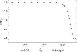
Figure 1: The SPT ground state energies from BCS to unitarity as a function of $\bar{V}_{0}$ for $N=12$.

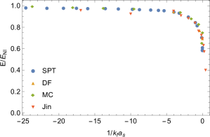
Figure 2: Ground state energies from BCS to unitarity as a function of $1/k_{f}a_{s}$. My SPT results are for $N=12$ and are compared to experimental jin3 , density functional (DF)adhikari1 and variational Monte Carlo results (MC)sanchez

.

III.2 Entropies from BCS to Unitarity

Although thermodynamic quantities have been well studied in the unitary regime, there are very few determinations of thermodynamic quantities across the BCS to unitarity transition. I have chosen to look at entropies across this transition since values for the entropy as a function of temperature have been calculated at several values of $1/k_{f}a_{s}$ using a T-matrix approachlevin2 . My approach uses a straightforward calculation of the partition function, summing over the spectrum of equally-spaced normal mode states that are chosen by the Pauli principle. Using the interpolated values of the scattering length obtained above, I have plotted values for the entropy at unitarity, $1/k_{f}a_{s}=0$ ($a_{s}=-\infty$), in Fig. 3 which agree well with theoreticalhu1 ; hu2 and experimental resultsnascimbene and at $1/k_{f}a_{s}=-0.5$ in Fig. 4 comparing to the theoretical results of Ref. levin2 .

The partition function becomes difficult to converge as the interparticle interaction decreases away from unitarity due to two effects: the narrowing of the frequencies and the increase in the value of the frequencies as they approach $2\omega_{ho}$ deep in the BCS regime. The larger frequency values mean that the individual terms of the partition function decrease their contribution to the total (a larger negative number in the numerator of each exponential) so more states are needed for convergence. The narrowing of the frequencies as the gaps shrink toward the BCS regime means that more states are becoming accessible at a given temperature which again increases the number of terms needed for convergence. This increase in the number of states as interactions weaken results in higher entropy values as can be seen in Fig. 4 for the weaker interactions at $1/k_{f}a_{s}=-0.5$ compared to unitarity results in Fig. 3. The number of states needed also increases as the temperature increases. These three effects combine to make it very challenging to calculate thermodynamic quantities accurately across the BCS to unitarity transition using straightforward summing over the available states. Alternative approaches to obtaining a converged partition function are complicated by the need to enforce the Pauli principle at each step.

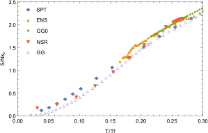
Figure 3: The SPT entropy for $N=20$ as a function of $T/T_{F}$ at unitarity is compared to experimental data: ENSnascimbene and theoretical results: NSR, GG0, and GGhu1 ; hu2 .

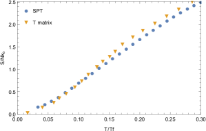
Figure 4: The entropy for $N=20$ as a function of $T/T_{F}$ for $1/k_{\mathtt{f}a}=0.5$. SPT results - blue dots, T matrix results - orange triangles from Ref. levin2

III.3 Estimate of Critical Temperatures from BCS to Unitarity

The critical temperature, $T_{C}$, is defined as the transition temperature from a normal fluid to a superfluid which exhibits long-range order due to a macroscopic occupation of the phonon ground state. This transition has been observed in the heat capacity whose thermodynamic expression involves a derivative with respect to the temperature. The heat capacity has a well-known, strong experimental signature in the unitary regime, the lambda transition, that has been studied extensively both experimentallythomas1 ; kinast1 ; thomas ; thomas2 ; zwierlein3 and theoreticallybulgac ; burovski2 ; hu2 ; hu5 . An estimate of the critical temperature in the unitary regime has also been extracted from measurements of the entropy as a function of temperature using the thermodynamic relation: $1/T=\partial{S}/\partial{E}$thomas .

Theoretically, the sudden change in thermodynamic properties as the ensemble becomes a superfluid is governed by the partition function and originates in the details of lowest terms including the size of the gap and the degeneracies of the lowest states. For a given spectrum, the partitioning of particles among the available energy levels depends on a single parameter, the temperature. As the temperature drops below the critical temperature, one expects to see the occupation in the phonon ground state increase rapidly due to the gap in the spectrum. This phenomenon is manifested by a sudden change in the value of certain observables such as the specific heat.

In an earlier SPT study in the unitary regimeemergence , a calculation of the specific heat clearly showed a cusp at the lambda transition, yielding a critical temperature of $(T/T_{F})_{C}=0.16$ which was significantly lower than previous results in the literature for trapped Fermi gases: $(T/T_{F})_{C}=0.19$nascimbene , $0.20$burovski2 , $0.21$hu2 ; hu5 ; haussmann3 , $(T/T_{F})_{C}=0.27$kinast1 ; hu5 ; bulgac , 0.29thomas ; hu5 . (See Fig. 5 reproduced from Fig. 12 in Ref. emergence .)

I have repeated this calculation for weaker interactions, $1/k_{f}a=-0.02$, $1/k_{f}a=-0.5$, and $1/k_{f}a=-1.0$, graphing the results in Fig. 6. As the interactions become weaker, the excitation gap decreases and the cusp signifying a transition to a superfluid quickly softens. While still visible at $1/k_{f}a=-0.02$ close to the unitary limit, the cusp is undetectable at a value of $1/k_{f}a\leq-0.5$ in the crossover region with just a slight inflection visible, and by $1/k_{f}a=-1.0$ no sign is detected. Thus, observing an experimental signature of this transition, certainly a definitive way to define the critical temperature, is not always possible in all regimes.

Theoretically, several approaches have been used to estimate the critical temperature at unitarity including a Monte Carlo studyburovski ; burovski2 that uses the behavior of a correlation function to determine an estimate of the critical temperature, and an auxiliary field quantum Monte Carlo approach that determines the critical temperature from a change in the behavior of the thermodynamic energy as a function of temperaturebulgac . Along the entire transition from BCS to unitarity, the critical temperature has been calculated by solving the gap equation self-consistently with the number equation under the condition that the order parameter goes to zero as the temperature approaches the critical temperature, $T_{C}$, from below, i.e. long-range order is lost. These equations have been solved at different levels of approximation from mean field which yields the well known BCS results to solutions in strongly interacting regimes near unitarity that include full fluctuationsgrava ; strinati1 ; melo .

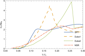
Figure 5: The heat capacity showing with cusp at the critical temperature, $T_{C}/T_{F}$ at unitarity comparing to experimental: Duke1thomas1 , Duke2kinast1 and theoretical results: NSRhu1 as a function of temperature.

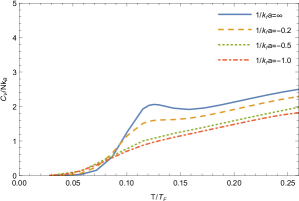
Figure 6: The heat capacity showing the softening of the cusp as the interparticle interaction decreases from a maximum at unitarity: blue line $1/k_{f}a=\infty$; orange dashed line $1/k_{f}a=-0.02$; green dotted line $1/k_{f}a=-0.5$; red dot dashed line $1/k_{f}a=-1.0$.

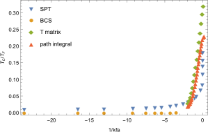
Figure 7: The critical temperature, $T_{C}/T_{F}$ as a function of $1/k_{f}a$ for 30 fermions compared to the BCS prediction valid for $1/k_{f}a\ll-1.0$ and theoretical resultsstrinati1 ; grava for $-1.0\leq 1/k_{f}a\ll 0$.

The SPT approach offers an alternative, straightforward way to estimate the critical temperature across the entire transition. Using the Pauli principle, the first excited state above the ground state can be determined along the transition. This excited state involves single particle excitations while the ground state is composed only of phonon normal modes. The difference between these two states gives an estimate of the critical temperature as simply the temperature equivalent: $E_{ex}-E_{gs}=k_{B}T_{C}$. This estimate is graphed in Fig. 7 normalized by the Fermi temperature $T_{F}$, $E_{F}=(3N)^{1/3}\hbar\omega_{ho}=k_{B}T_{F}$, and compared to other theoretical results in the region near unitarity and to the BCS expression, $T_{C}/T_{F}=0.277\exp(\pi/(2k_{f}a)$ valid for $1/k_{f}a\ll-1.0$. The SPT results are slightly higher than the BCS results, showing a gradual increase from the deep BCS regime toward unitarity and then a rapid increase for $1/k_{f}a\geq-1.0$ as the interactions approach unitarity. The curve converges at unitarity at $(T/T_{F})_{C}=0.18$ in reasonable agreement with several other theoretical approachesnascimbene ; burovski2 ; hu2 ; hu5 ; haussmann3

III.4 The breathing mode frequency from BCS to Unitarity.

Investigating collective excitation modes has long been used to gain insight into the behavior of many-body systems. The excitation frequencies of ultracold Fermi gases have been studied intensely across the BEC-BCS transition. The radial compression or “breathing” mode in a cylindrical potential has been of particular interest due to a surprising feature observed in the regime of strong interactions, specifically an abrupt decrease in the frequency near unitaritythomas1 ; bartenstein ; grimm1 ; grimm2 . This minimum has been confirmed theoreticallytosi ; zubarev ; salasnich .

The microscopic basis for this minimum in the breathing mode has been attributed to the formation of Cooper pairs as unitarity is approached which decreases the frequency as the gas becomes more compressibletosi . It has also been suggested from the observation of this minimum coupled with an analysis of the corresponding damping time, that this feature could be a signature of a transition from a superfluid to a collisionless phasebartenstein ; thomas1 as interactions weaken toward the independent particle regime.

In a recent paper, SPT was used to study the five analytic normal mode excitation frequencies in a symmetric trap across the transition from BCS to unitarityprafreq . This study revealed that unlike the angular frequencies which converged smoothly to integer multiples of the trap frequency, the two radial frequencies went through a minimum as unitarity is approached and then continued to increase suggesting that these first order frequencies might not be fully converged at unitarity. (See Fig. 2 in Ref. prafreq .)

In Fig. 8, I have regraphed in the SPT radial breathing normal mode frequency $\omega_{{\bf 0}^{-}}$ as a function of the parameter $1/N^{1/6}a$ through the region of the minimum and compared to these earlier results. Fig. 8 clearly shows a minimum for the SPT frequency between $1/N^{1/6}a=-1.0$ and unitarity, $1/N^{1/6}a=0$, in close agreement with these previous experimental and theoretical resultsgrimm2 ; thomas1 ; tosi ; zubarev ; salasnich . The SPT minimum is broad in Fig. 2 in Ref. prafreq graphed as a function of $\bar{V}_{0}$ on a log scale spanning several orders of magnitude from $\bar{V}_{0}=10^{-3}$ to $\bar{V}_{0}=1.0$, but is quite sharp when graphed as a linear function of $-1/N^{1/6}a$ in Fig. 8 where it maps into a small region between $1/N^{1/6}a=-1.0$ and $1/N^{1/6}a=0$.

The other SPT radial excitation, $\omega_{{\bf 1}^{-}}$, which is a single-particle excitation also clearly shows a minimum when graphed as a function of $\bar{V}_{0}$ in Fig. 2 of Ref. prafreq . When regraphed as a function of $1/N^{1/6}a$, this minimum is visible, but quite small.

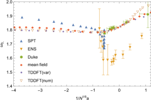
Figure 8: Excitation frequency for the radial breathing mode in a symmetric trap as a function of $1/N^{1/6}a$ for 30 fermions showing the minimum as unitarity is approached that is seen theoreticallyzubarev ; salasnich ; tosi and experimentally in cylindrical trapsgrimm2 ; thomas1

The analytic form of the SPT normal modes offers an opportunity to analyze the microscopic dynamics responsible for this minimum. By tracking the contribution of different terms in the Hamiltonian to the analytic expression for the frequency across the transition, one can understand what is happening microscopically to produce this minimum. The following analysis is based on previous work in Ref prafreq .

Understanding the microscopic dynamics of the minimum in the radial breathing frequency.

The analytic expressions for the frequencies have been studied across the transition from BCS to unitarityprafreq . Appendix C in Ref. prafreq has an analysis of the radial breathing frequency $\omega_{{\bf 0}^{-}}$ in terms of the $FG$ matrix elements from the terms in the first-order Hamiltonian (Eq. (15)). The formula derived in this Appendix for $\omega_{{\bf 0}^{-}}$ in terms of the $FG$ elements is:

$$\omega_{{0}^{-}}\approx\sqrt{G_{a}F_{a}+(N-1)G_{a}F_{b}}\\$$ (26)

where $G_{a}=1$, $F_{a}$ and $F_{b}$ involve derivatives of $\bar{V}_{\mathtt{eff}}$ (See Eq. 10.) which is a sum of the confining potential $\bar{V}_{\mathtt{conf}}$, the centrifugal potential $\bar{V}_{\mathtt{cent}}=\bar{U}$, and the interparticle interaction potential $\bar{V}_{\mathtt{int}}$:

$$\bar{V}_{\mathtt{eff}}=\bar{U}+\bar{V}_{\mathtt{conf}}+\bar{V}_{\mathtt{int}}.$$ (27)

yielding three terms for $F_{a}$: $F_{a}=F_{a}^{\mathtt{cent}}+F_{a}^{\mathtt{conf}}+F_{a}^{\mathtt{int}}$ and one nonzero term for $F_{b}$ involving the interaction potential: $F_{b}=F_{b}^{\mathtt{int}}$. The term $F_{a}^{\mathtt{conf}}$ is a constant equal to 1. All the terms are explicitly defined in Appendix B in Ref. prafreq .

As in the analysis of the angular frequencies in Section VI of Ref. prafreq , it is useful to track the magnitude of $\gamma_{\infty}$, the angle cosine of each pair of particles at the minimum of the maximally-symmetric structure at large dimension. Early dimensional scaling work identified a nonzero value of this parameter as a signature of the existence of correlation between the particles. Mean field results have $\gamma_{\infty}=0$ corresponding to no correlation between the particles, while increasing values of $\gamma_{\infty}$ indicated stronger and longer-range correlation effects existed.

Consider the independent particle limit, i.e. collisionless regime, with no interparticle interactions so $\bar{V}_{0}=0$ and thus no correlations between the particles i.e. $\gamma_{\infty}=0$ so only the harmonic trap is affecting the particles which of course are also obeying the Pauli principle. Most of the terms in the expression for $\bar{\omega}_{{0}^{-}}$ in Eq. (26) are zero. The only non-zero terms are $F_{a}^{\mathtt{conf}}=1$ from the trap potential and $F_{a}^{\mathtt{cent}}=3$ which originates in the kinetic energy, giving $F_{a}=4$, $F_{b}=0$ so $\omega_{{\bf 0}^{-}}=2\omega_{ho}$ as expected and confirmed in the laboratory. (See Appendix F in Ref. prafreq .) As interactions are introduced, $\gamma_{\infty}$ assumes a small nonzero value, signaling the existence of weak correlations. This nonzero value means that all of the terms in the expression for $\bar{\omega}_{{0}^{-}}$ are nonzero. $F_{a}^{\mathtt{cent}}$ begins to decrease, while $F_{a}^{\mathtt{int}}$ and $F_{b}^{\mathtt{int}}$ increase. Along the BCS to unitarity transition, the value of $\bar{\omega}_{{0}^{-}}$ is a balance between the centrifugal term which is decreasing and the interaction terms which are increasing as interactions ($\bar{V}_{0}$) and correlations ($\gamma_{\infty}$) both increase from BCS toward unitarity. The minimum in the frequency occurs from the continued decrease in the centrifugal terms just before the increase in the interaction terms dominates.

Microscopically, one can understand what is happening from this analysis of the Hamiltonian terms. The increase in the correlated motion of the particles as tracked by the increase in $\gamma_{\infty}$ minimizes the interparticle interactions resulting in slower oscillations of the breathing mode. Eventually the increase in $\bar{V}_{0}$, i.e. the increased strength of the interparticle interactions will, of course, lead to more rapid oscillations i.e. an increase in the frequency as unitarity is approached. The gradual decrease seen when $\bar{\omega}_{{0}^{-}}$ is graphed as a function of $\bar{V}_{0}$ in Ref. prafreq appears as a sudden, quite narrow dip in the frequency when graphed as a function of $1/(N^{1/6}a)$. This is due to the rapidly changing scattering length in this region as unitarity is approached. In summary, the minimum is the result of two competing factors which affect the microsopic behavior: the increase in correlation which minimizes the interparticle interactions thus slowing down the frequency of the oscillations and second, the increasing strength of the interparticle interactions which eventually dominates and speeds up the frequency of the oscillations.

IV Summary and Conclusions

In this study, I have explored the ability of normal modes to describe the behavior of ultracold Fermi gases including superfluidity across the BCS to unitarity transition without assuming Cooper pairing. In particular, I have calculated the following properties: ground state energies, thermodynamic entropies, critical temperatures and the radial breathing frequency across this transition using normal modes and compared to available experimental and theoretical results.

An earlier study that looked at the behavior of the SPT normal mode frequencies across this transition found that the frequencies were capable of describing the emergence of excitation gaps from very small gaps deep in the BCS regime to a maximum at unitarity as observed experimentally. In addition, they provided insight into the microscopic dynamics responsible for the universal behavior at unitarity. This was possible due to the analytic forms of both the $N$-body normal mode frequencies and their coordinates.

The success of this earlier study motivated the current exploration of additional properties across the transition. This study has yielded close agreement with both experimental and theoretical results for the ground state energies, thermodynamic entropies and critical temperatures at weaker interactions away from unitarity. These calculations tested the lowest frequencies relevant to ultracold systems as well as the spectrum of frequencies needed for the partition function. In all these calculations, the Pauli principle has played a central role in choosing the states that contribute to these properties. The final study involved a single frequency, the breathing frequency, which did not contribute to the earlier studies due to its larger value. The observed dip in this SPT frequency near unitarity was in close agreement with results first observed in the laboratory and later confirmed theoretically, suggesting that the first-order SPT Hamiltonian that produces this frequency contains sufficient physics to describe this transition.

The normal coordinates constitute beyond-mean-field, analytic solutions to a many-body Hamiltonian and offer insight microscopically into the evolution of properties across the BCS to unitarity transition. The analytic forms for the frequencies and coordinates allow a detailed look at the dynamics by tracking the effect of Hamiltonian terms across the transition. As correlations increase toward unitarity as tracked by the parameter $\gamma_{\infty}$, the dependence of properties on the details of the interparticle interactions is minimized consistent with the universal behavior which is also seen at the independent particle limit. The Pauli principle, of course, is dominating the dynamics at both limits underpinning the universal behavior in these regimes.

The results of this study are based on an exact solution of the first-order equation of SPT perturbation theory which contains beyond-mean-field effects. Higher order terms which have been formulated, but not implemented, are not included. These terms could become significant in some regimes changing the dynamics. The SPT formalism also does not offer a mechanism for the two-body pairing that occurs as the ensemble transitions to the BEC regime.

The successful description of these properties across the BCS to unitarity transition using these first-order normal mode solutions supports my earlier conclusions that normal modes are a viable model of superfluidity across a broad range of interparticle interaction strengths and represent an interesting alternative to Cooper pairing models.

V Acknowledgments

I am grateful to the National Science Foundation for financial support under Grant No. PHY-2011384.

References

- (1) M. Greiner, C.A. Regal, and D.S. Jin, Nature 426, 537(2003).
- (2) M.W. Zwierlein, C.A. Stan, C.H. Schunck, S.M.F. Raupach, S. Gupta, Z. Hadzibabic, and W. Ketterle, Phys. Rev. Lett. 91, 250401 (2003).
- (3) S. Jochim, M. Bartenstein, A. Altmeyer, G. Hendl, S. Riedl, C. Chin, J. Hecker Denschlag, R. Grimm, Science 302, 2101 (2003).
- (4) J. Kinast, S.L. Hemmer, M.E. Gehm, A. Turlapov and J.E. Thomas, Phys. Rev. Lett. 92, 150402 (2004).
- (5) T. Bourdel, L. Khaykovich, J. Cubizolles, J. Zhang, F. Chevy, M. Teichmann, L. Tarruell, S.J.J.M.F. Kokkelmans and C. Salomon, Phys. Rev. Lett. 93, 050401 (2004).
- (6) C.A. Regal, M. Greiner, and D.S. Jin, Phys. Rev. Lett. 92, 040403(2004).
- (7) M.W. Zwierlein, C.A. Stan,C.H. Schunck,S.M.F. Raupach, A.J. Kerman, and W. Ketterle, Phys. Rev. Lett. 92, 120403(2004).
- (8) C. Chin, M. Bartenstein, A. Altmeyer, S. Riedl, S. Jochim, Hecker-Denschlag and R. Grimm, Science 305, 1128 (2004).
- (9) G.B. Partridge, K.E. Strecker, R.I. Kamar, M.W. Jack and R.G. Hulet, Phys. Rev. Lett. 95, 020404 (2005).
- (10) J. Bardeen, L.N. Cooper, and J.R. Schrieffer, Phys. Rev. 108, 1175 (1957).
- (11) A.J. Leggett, In Modern Trends in the Theory of Condensed Matter. Proceedings of the XVIth Karpacz Winter School of Theoretical Physics, Karpacz, Poland, pgs. 13-27, Springer-Verlag, Berlin, 1980.
- (12) A.J. Leggett, Rev. Mod. Phys. 73, 307(2001).
- (13) D.M. Eagles, Phys. Rev. 186, 456 (1969).
- (14) P. Nozieres and S. Schmitt-Rink, J. Low Temp. Phys .59, 195 (1985).
- (15) S. Giorgini, L.P. Pitaevskii, and S. Stringari, Rev. Mod. Phys. 80, 1215(2008).
- (16) M. Randeria and E. Taylor, Ann. Rev. Condensed Matter Phys. 5, 209(2014).
- (17) D.K. Watson, Phys. Rev. A 92, 013628 (2015).
- (18) D.K. Watson, J. Phys. B. 52, 205301 (2019).
- (19) D.K. Watson, Phys. Rev. A 104, 033320 (2021).
- (20) M. Dunn, D.K. Watson, and J.G. Loeser, Ann. Phys. (NY), 321, 1939 (2006).
- (21) W.B. Laing, M. Dunn, and D.K. Watson, J. of Math. Phys. 50, 062105 (2009).
- (22) D.L. Rousseau, R.T. Bauman, S.P.S. Porto, J. Ramam Spect., 10, 253(1981).
- (23) K. D. Kokkolas, Class. Quantum Grav. 8, 2217 (1991).
- (24) M.J. Clement, App J. 249, 746(1981).
- (25) N. Zagar, J. Boyd, A. Kasaara, J. Tribbia, E. Kallen, H. Tanaka, and J.-i Yano, Bull. Am. Meteor. Soc. 97 (2016).
- (26) S.C. Webb, Geophys.J. Int. 174, 542(2008).
- (27) B.V. Sanchez, J. Marine Geodesy 31, 181(2008).
- (28) J. Lee, K.T. Crampton, N. Tallarida, and V.A.Apkarian, Nature 568, 78(2019).
- (29) L. Fortunato, EPJ Web of Conferences 178, 02017 (2018).
- (30) E.C. Dykeman and O.F. Sankey, J. Phys.:Condens. Matter 22, 423202(2010).
- (31) M. Coughlin and J. Harms, arXiv:1406.1147v1 [gr-qc] (2014).
- (32) R.M. Stratt, Acc. Chem. Res. 28, 201(1995).
- (33) C.R. McDonald, G. Orlando, J.W. Abraham, D. Hochstuhl, M. Bonitz, and T. Brabec, Phys. Rev. Lett. 111, 256801 (2013); F. Dalfovo, S. Giorgini, L.P. Pitaevskii, and S. Stringari, Rev. Mod. Phys. 71, 463(1999); D. Jaksch, C. Bruder, J.I. Cirac, C.W. Gardiner, and P. Zoller, Phys. Rev. Lett. 81, 3108(1998); H. Dong, W. Zhang, L. Zhou and Y. Ma, Sci. Rep. 5, 15848; doi: 10.1038/srep15848(2015).
- (34) H.C. Nagerl, C. Roos, H. Rohde, D. Leibfried, J. Eschner, F. Schmidt-Kaler and R. Blatt, Fortschr. Phys. 48, 623 (2000).
- (35) B.A. McKinney, M. Dunn, D.K. Watson, and J.G. Loeser, watson Ann. Phys. 310, 56 (2003).
- (36) B.A. McKinney, M. Dunn, D.K. Watson, Phys. Rev. A 69, 053611 (2004).
- (37) W.B. Laing, M. Dunn, and D.K. Watson, Phys. Rev. A 74, 063605 (2006).
- (38) W.B. Laing, D.W. Kelle, M. Dunn, and D.K. Watson, J Phys A 42, 205307 (2009).
- (39) M. Dunn, W.B. Laing, D. Toth, and D.K. Watson, Phys. Rev A 80, 062108 (2009).
- (40) Y. K. Liu, M. Christandl, and F. Verstraete, Phys. Rev. Lett. 98, 110503 (2007).
- (41) A. Montina, Phys. Rev. A 77, 022104 (2008).
- (42) D.K. Watson and M. Dunn, Phys. Rev. Lett. 105, 020402 (2010).
- (43) D.K. Watson and M. Dunn, J. Phys. B 45, 095002 (2012).
- (44) Dimensional Scaling in Chemical Physics, edited by D.R. Herschbach, J. Avery, and O. Goscinski (Kluwer, Dordrecht, 1992).
- (45) New Methods in Quantum Theory, edited by C. A. Tsipis, V. S. Popov, D. R. Herschbach, and J. Avery, NATO Conference Book, Vol. 8. (Kluwer Academic, Dordrecht, Holland).
- (46) J.G. Loeser, J. Chem. Phys. 86, 5635 (1987).
- (47) S. Kais and D.R. Herschbach, J. Chem. Phys. 100, 4367 (1994).
- (48) S. Kais and R. Bleil, J. Chem. Phys. 102, 7472 (1995).
- (49) D.K. Watson, Phys. Rev. A 93, 023622 (2016).
- (50) D.K. Watson, Phys. Rev. A 96, 033601(2017).
- (51) D.K. Watson, Ann. Phys. 419, 168219 (2020).
- (52) S.K. Adhikari, Phys. Rev. A 79, 023611(2009).
- (53) X.-J. Liu, H. Hu,and P.D. Drummond, Phys. Rev. Lett. 102, 160401 (2009).
- (54) X.-J. Liu, H. Hu, and P.D. Drummond, Phys. Rev. A 82, 023619 (2010).
- (55) X.-J. Liu, H. Hu, and P.D. Drummond, Phys. Rev. B 82, 054524 (2010).
- (56) T. Grining, M. Tomza, M. Lesiuk, M. Przybytek, M. Musial, R. Moszynski, M. Lewenstein, and P. Massignan, Phys. Rev. A 92, 061601(R) (2015).
- (57) D. Blume, Physics 3, 74 (2010).
- (58) D.Blume, Rep. Prog. Phys. 75, 046401 (2012).
- (59) J. Levinsen, P. Massignan, S. Endo, and M.M. Parish, J. Phys. B 50, 072001 2017).
- (60) J. Avery, D.Z. Goodson, D.R. Herschbach, Theor. Chim. Acta 81, 1 (1991).
- (61) W.B. Laing, M. Dunn, and D.K. Watson, EPAPS Document Number E-JMAPAQ-50-031904.
- (62) E. B. Wilson, Jr., J. Chem. Phys. 9, 76 (1941).
- (63) E.B. Wilson, Jr., J.C. Decius, P.C. Cross, Molecular vibrations: The theory of infrared and raman vibrational spectra. McGraw-Hill, New York, 1955.
- (64) M. Hamermesh, Group theory and its application to physical problems, Addison-Wesley, Reading, MA, 1962.
- (65) See for example Ref. dcw , Appendix XII, p. 347.
- (66) L.D. Landau, “The Theory of a Fermi Liquid,” Sov. Phys. 3, 920-925 (1956); “Oscillations in a Fermi Liquid,” ibid. 5, 101-108 (1957).
- (67) J. Carlson and S. Gandolfi, Phys. Rev. A 90 011601(R) (2014).
- (68) S.K. Adhikari, Phys. Rev. A 79, 023611 (2009).
- (69) D. Blume, J. von Stecher, and C.H. Greene, Phys. Rev. Lett. 99, 233201 (2007).
- (70) S.Y. Chang and G. F. Bertsch, New J. Phys. 11, 023011 (2007).
- (71) T. D. Lee et al., Phys. Rev. 105, 1119(1957).
- (72) R. Jáuregui, R. Paredes, and G. Toledo Sánchez, Phys. Rev. A 76, 011604(R) (2007).
- (73) J.T. Stewart, J.P. Gaebler, C.A. Regal and D.S. Jin, Phys. Rev. Lett. 97, 220406 (2006).
- (74) D.T. Son, arXiv:0707.1851 [cond-mat.other], 2007.
- (75) Q. Chen, J. Stajic, and K. Levin, Phys. Rev. Lett. 95, 260405 (2005).
- (76) H. Hu, X.-J. Liu, and P.D. Drummond, Phys. Rev. A 73, 023617 (2006).
- (77) H. Hu, X.-J. Liu, and P.D. Drummond, New Journal of Physics 12, 063038 (2010).
- (78) S. Nascimbene et al. Nature(London) 463, 1057(2010).
- (79) L. Luo, B. Clancy, J. Joseph, J. Kinast, and J. E. Thomas, Phys. Rev. Lett., 98,080402 (2007).
- (80) L. Luo, J.E. Thomas, J. Low Temp. Phys. 154, 1 (2009).
- (81) J.Kinast, A. Turlapov, J.E. Thomas, Q. Chen, J. Stajic, K. Levin, Science 307, 1296 (2005).
- (82) M. J. H. Ku, A. T. Sommer, L. W. Cheuk, and M. W. Zwierlein, Science, 335(6068), 563-567 (2012).
- (83) A. Bulgac, J.E. Drut, and P. Magierski, Phys. Rev. Lett 99, 120401 (2007).
- (84) E. Burovski, N. Prokof’ev, B. Svistunov and M. Troyer, New J. of Phys. 8, 153 (2006).
- (85) H. Hu, X.-J. Liu, and P.D. Drummond, Phys. Rev. A 77, 061605(R) (2008).
- (86) R Haussmann and W Zwerger, Phys. Rev. A 78, 063602 (2008).
- (87) E. Burovski, N. Prokof’ev, B. Svistunov and M. Troyer, Phys. Rev. Lett. 96, 160402 (2006).
- (88) A. Perali, P. Pieri, L. Pisani, and G.C. Strinati, Phys. Rev. Lett. 92,220404 (2004).
- (89) L. Dell’Anna and S. Grava, Condens. Matter 6,16(2021).
- (90) C.A.R. Sá de Melo, M. Randeria, and J. R. Engelbrecht, Phys. Rev. Lett. 71, 3202(1993).
- (91) R. Grimm, “Proceedings of the International School of Physics “Enrico Fermi”, Volume 164: Ultracold Fermi Gases, p 413-462, 2007.
- (92) M. Bartenstein, A. Altmeyer, S. Riedl, S. Jochim, (2004).
- (93) Y.E. Kim and A.L. Zubarev, Phys. Rev. A 70, 033612(2004).
- (94) N. Manini and L. Salasnich, Phys Rev. A 71, 033625(2005).
- (95) H. Hu, A. Minguzzi, X-J Liu, and M.P. Tosi, Phys. Rev. Lett. 93, 190403(2004).