Sampling Enclosing Subgraphs for Link Prediction

Abstract.

Link prediction is a fundamental problem for graph-structured data (e.g., social networks, drug side-effect networks, etc.). Graph neural networks have offered robust solutions for this problem, specifically by learning the representation of the subgraph enclosing the target link (i.e., pair of nodes). However, these solutions do not scale well to large graphs as extraction and operation on enclosing subgraphs are computationally expensive, especially for large graphs. This paper presents a scalable link prediction solution, that we call ScaLed, which utilizes sparse enclosing subgraphs to make predictions. To extract sparse enclosing subgraphs, ScaLed takes multiple random walks from a target pair of nodes, then operates on the sampled enclosing subgraph induced by all visited nodes. By leveraging the smaller sampled enclosing subgraph, ScaLed can scale to larger graphs with much less overhead while maintaining high accuracy. ScaLed further provides the flexibility to control the trade-off between computation overhead and accuracy. Through comprehensive experiments, we have shown that ScaLed can produce comparable accuracy to those reported by the existing subgraph representation learning frameworks while being less computationally demanding.

1. Introduction

Graph-structured data such as user interactions, collaborations, protein-protein interactions, drug-drug interactions are prevalent in natural and social sciences. Link prediction—a fundamental problem on graph-structured data—intends to quantify the likelihood of a link (or interaction) occurring between a pair of nodes (e.g., proteins, drugs, etc.). Link prediction has many diverse applications such as predicting drug side effects, drug-repurposing (Gysi et al., 2021), understanding molecule interactions (Huang et al., 2020), friendship recommendation (Chen et al., 2020), and recommender systems (Ying et al., 2018).

Many solutions to link prediction problem (Liben-Nowell and Kleinberg, 2007; Lü and Zhou, 2011; Martínez et al., 2016; Wang et al., 2015; Kumar et al., 2020) has been proposed ranging from simple heuristics (e.g., common neighbors, Adamic-Adar (Adamic and Adar, 2003), Katz (Katz, 1953)) to graph neural networks (GNNs) (Kipf and Welling, 2016; Zhang and Chen, 2018; Pan et al., 2022; Hao et al., 2020; Cai and Ji, 2020; Cai et al., 2021). Among these solutions, GNNs (Hamilton, 2020; Wu et al., 2020; Zhou et al., 2020) have emerged as the widely-accepted and successful solution for learning rich latent representations of graph data to tackle link prediction problems. The early GNNs focused on shallow encoders (Perozzi et al., 2014; Grover and Leskovec, 2016) in which the latent nodes’ representations was first learnt through a sequence of random walks, and then a likelihood of a link is determined by combining its two-end nodes’ latent representations. However, these shallow encoders were limited by not incorporating nodal features and their incompatibility with inductive settings as they require that all nodes are present for training. These two challenges were (partially) addressed with the emergence of message-passing graph neural networks (Kipf and Welling, 2017; Hamilton et al., 2017; Xu et al., 2019). These advancements motivate the research on determining and extending the expressive power of GNNs (You et al., 2021; Bevilacqua et al., 2022; You et al., 2019; Zhang et al., 2018; Zeng et al., 2021; Fey et al., 2021) for all downstream tasks of link prediction, node classification, and graph classification. For link prediction, subgraph-based representation learning (SGRL) methods (Zhang and Chen, 2018; Li et al., 2020; Pan et al., 2022; Cai and Ji, 2020; Cai et al., 2021)—by learning the enclosing subgraphs around the two-end nodes rather than independently learning two end-node’s embedding—have improved GNNs expressive power, and offered state-of-the-art solutions. However, these solutions suffer from the lack of scalability, thus preventing them to be applied to large-scale graphs. This is primarily due to the computation overhead in extracting, preprocessing, and learning (large) enclosing subgraphs for any pair of nodes. We focus on addressing this scalability issue.Contribution. We introduce Sampling Enclosing Subgraph for Link Prediction (ScaLed) to extend SGRL methods and enhance their scalability. The crux of ScaLed is to sample enclosing subgraphs using a sequence of random walks. This sampling reduces the computational overhead of large subgraphs while maintaining their key structural information. $S{ca}L{ed}$ can be integrated into any GNN, and also offers parallelizability and model compression that can be exploited for large-scale graphs. Furthermore, the two hyperparameters, walk length and number of walks, in ScaLed provides a way to control the trade-off between scalability and accuracy, if needed. Our extensive experiments on real-world datasets demonstrate that ScaLed produces comparable results to the state-of-the-art methods (e.g, SEAL (Zhang and Chen, 2018)) in link prediction, but requiring magnitudes less training data, time, and memory. ScaLed combines the benefits of SGRL framework and random walks for link prediction. Other related work. Graph neural networks have benefited from sampling techniques (e.g, node sampling (Hamilton et al., 2017; Chen et al., 2018a; Zou et al., 2019) and graph sampling (Zeng et al., 2020)) to make training and inference more scalable on large graphs. Also, historical embeddings (Chen et al., 2018b; Fey et al., 2021) have shown promises in speeding up the aggregation step of GNNs for the downstream task of node classification (Chen et al., 2018a; Chiang et al., 2019; Fey et al., 2021). However, little attention is given to scaling up of SGRL methods for link prediction; except a few exceptions (Yin et al., 2022; Zeng et al., 2021), which do not benefit from GNNs for subgraph learning (Yin et al., 2022) or is restricted to learning on individual nodes (Zeng et al., 2021).

2. Link Prediction

We consider an undirected graph $G=(V,E,\mathbf{A})$ where $V=[n]$ is the set of $n$ nodes (e.g., individuals, proteins, etc), $E\subseteq V\times V$ represents the edge set (e.g., friendship relations or protein-to-protein interactions) and the tensor $\mathbf{A}\in\mathbb{R}^{n\times n\times d}$ contains all nodes’ attributes (e.g., user profiles) and edges’ attributes (e.g, the strength or type of interactions). For each node $v\in V$, its attributes (if any) are stored in the diagonal component $\mathbf{A}_{vv.}$ while the off-diagonal component $\mathbf{A}_{uv.}$ can have the attributes of an edge $(u,v)$ if $(u,v)\in E$; otherwise $\mathbf{A}{{}_{uv.}}=\mathbf{0}$.

Link Prediction Problem. Our goal in link prediction is to infer the presence or absence of an edge between a pair of target nodes given the observed tensor $\mathbf{A}$. The learning problem is to find a likelihood (or scoring) function $f$ such that it assigns interaction likelihood (or score) $\hat{A}_{uv}$ to each target pair of nodes $(u,v)\notin E$, whose relationships to each other are not observed. Larger $\hat{A}_{uv}$ indicates a higher chance of $(u,v)$ forming a link or missing a link. The function $f$ can be formulated as $\hat{A}_{uv}$ = $f(u,v,\mathbf{A}|\boldsymbol{\theta})$ with $\boldsymbol{\theta}$ denoting the model parameters. Most link prediction methods differ from each other in the formulation of the likelihood function $f$ and its assumptions. The function $f$ can be some parameter-free predefined heuristics (Adamic and Adar, 2003; Page et al., 1999; Katz, 1953) or learned by a graph neural network (Kipf and Welling, 2017; Hamilton et al., 2017; Veličković et al., 2018; Xu et al., 2019) or any other deep learning framework (Yin et al., 2022). The likelihood function formulation also varies based on its computation requirement on the maximum hop of neighbors of target nodes. For example, first-order heuristics (e.g., common neighbors and preferential attachment (Barabási and Albert, 1999)) only require the direct neighbors while graph neural networks methods (Kipf and Welling, 2016; Hamilton et al., 2017) and high-order heuristics (e.g., Katz (Katz, 1953), rooted PageRank (Brin and Page, 2012)) require knowledge of the entire graph.

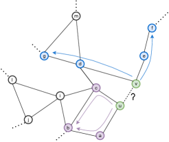
(a) Original graph with target nodes $u,v$.

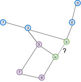
(b) Induced subgraph with labels.

Figure 1. The ScaLed model: (a) the random walks from target nodes $u$ (blue arrows) and $v$ (purple arrows) ; and (b) the induced sampled enclosing subgraph with DRNL labels.

3. The ScaLed model

After describing the SEAL link prediction model and its variants, we detail how our proposed ScaLed model extends these models to maintain their prediction power but offer better scalability.

SEAL and its variants. Rather than learning the target nodes’ embeddings independently (as with Graph Convolutional Network (Kipf and Welling, 2017) or GraphSAGE (Hamilton et al., 2017)), SEAL (Zhang and Chen, 2018) focuses on learning the enclosing subgraph of a pair of target nodes to capture their relative positions to each other in the graph:

Definition 1 (Enclosing Subgraph (Zhang and Chen, 2018)).

Given a graph $G$, the $h$-hop enclosing subgraph around target nodes (u,v) is the subgraph $G_{uv}^{h}$ induced from $G$ with the set of nodes $\{j\|d(j,x)\leq h\ or\ d(j,y)\leq h\}$, where $d(i,j)$ is the geodesic distance between node $i$ and $j$.

In SEAL, for each pair of the target nodes $(u,v)$, their enclosing subgraph $G_{uv}^{h}$ is found and extracted with two $h$-hop Breadth-First Search (BFS), where each BFS starts from $u$ and $v$. The nodes in the extracted enclosing subgraph are also augmented with labels indicating their distances to the target pair of nodes using the Double-Radius Node Labeling (DRNL) hash function (Zhang and Chen, 2018):

(1) $$DRNL(x,G_{uv}^{h})=1+min\left(d_{xu},d_{xv}\right)+\lfloor d^{\prime}/2\rfloor\lceil d^{\prime}/2-1\rceil,$$

where $x$ represents the nodes in the subgraph $G_{uv}^{h}$, $d_{xu}$ is the geodesic distance of $x$ to $u$ in $G_{uv}^{h}$ when node $v$ is removed, and $d^{\prime}=d_{xu}+d_{xv}$. Note that the distance of $x$ to each target node $u$ is calculated in isolation by removing the other target node $v$ from the subgraph. The target nodes are labeled as 1 and a node with $\infty$ distance to at least one of the target nodes is given the label $0$. Each node label is then represented by its one-hot encoding, and expands the initial node features, if any. The subgraph $G_{uv}^{h}$ along with the augmented nodal features is fed into a graph neural network, which predicts the presence or absence of the edge. In SEAL, the link prediction is treated as a binary classification over the enclosing subgraphs by determining if the enclosing subgraph will be closed by a link between the pair of target nodes or not. Thus, SEAL uses a graph pooling mechanism (e.g., SortPooling (Zhang et al., 2018)) to compute the enclosing subgraph representation for the classification task. Other variants of SEAL (e.g., DE-GNN (Li et al., 2020) and WalkPool (Pan et al., 2022)) have replaced either its DRNL labeling method (Li et al., 2020) or graph aggregation method (Li et al., 2020) with some other alternatives to improve its expressivness power. However, SEAL and these variants all suffer from the scalability issue as the subgraph size grows exponentially with the hop size $h$, and large-degree nodes (e.g., celebrities) possess very large enclosing subgraphs even for a small $h$. To address these scalablity issues, we propose Sampling Enclosing Subgraph for Link Prediction (ScaLed).

ScaLed. Observing that the computational bottleneck of SEAL and its variants originates from the exponential growth and the size of enclosing subgraphs, we propose Sampled Enclosing Subgraphs with more tractable sizes:

Definition 2 (Random Walk Sampled Enclosing Subgraph).

Given a graph $G$, the random-walk sampled $h$-hop enclosing subgraph around target nodes (u,v) is the subgraph $\hat{G}_{uv}^{h,k}$ induced from $G$ with the set of nodes $\hat{V}^{h,k}_{uv}\in W_{u}^{h,k}\cup W_{v}^{h,k}$, where $W_{i}^{h,k}$ is the set of nodes visited by $k$ many h-length random-walk(s) from node $i$.

Figure 1(b) illustrates sampled enclosing subgraph of the target pair of $(u,v)$ for the original graph in Figure 1(a), where $h=2$ and $k=2$. Here, $W_{v}^{h,k}=\{v,d,e,f,g\}$ and $W_{u}^{h,k}=\{u,a,b,c\}$, resulting in $\hat{V}^{h,k}_{uv}=\{a,b,c,d,e,f,g,u,v\}$. The included subgraph in Figure 1(b) contains all nodes and edges between nodes in $\hat{V}^{h,k}_{uv}$.

Comparing Definitions 1 and 2, a few important observations can be made: (i) the sampled enclosing subgraph $\hat{G}_{uv}^{h,k}$ is the subgraph of the enclosing subgraph $G_{uv}^{h}$, as the $h$-length random walks can not reach a node further than $h$-hop away from the starting node; (ii) the size of the sampled subgraph is bounded to $O(hk)$ and controlled by these two parameters compared to the exponential growth of enclosing subgraphs with $h$ in Definition 1. ScaLed, by replacing the dense enclosing subgraphs with their sparse (sub)subgraphs, offers scalability, while still providing flexibility to control the extent of sparsity and scalability with its sampling parameters $h$ and $k$.

The ScaLed model can use any labeling trick (e.g., DRNL, zero-one labeling, etc.) (Zhang et al., 2021) to encode the distances between target nodes and other nodes in the sampled subgraphs; see Figure 1(b) for an example. Similar to SEAL, the one-hot encoding of the distance labels along with the nodal features (if any) of the nodes in the sampled subgraph are fed into a graph neural network with graph pooling operation (e.g., DGCNN with SortPooling operation (Zhang et al., 2018)) for the classification task. The ScaLed model offers easy plug-and-play modularity into most graph neural networks (e.g., GCN (Kipf and Welling, 2017), GIN (Xu et al., 2019), GraphSAGE (Hamilton et al., 2017), DGCNN (Zhang et al., 2018), etc.), and can also be used alongside any regularization technique or loss function.

Although random walks have been used in unsupervised latent learning of graph data (Perozzi et al., 2014; Grover and Leskovec, 2016), ScaLed has used them differently for sparsifying the enclosing subgraphs to enhance scalability. This random-walk subgraph sampling technique can be incorporated into any other subgraph representation learning task to improve scalability by increasing sparsity of the subgraph. This technique does not incur much computational overhead, can be viewed as a preprocessing step, and can benefit from parallelizability. Furthermore, random-walk sampled subgraphs have controllable size and and do not grow exponentially with $h$.

Dataset	# Nodes	# Edges	Avg. Deg.	# Features
USAir	332	2126	12.81	NA
Celegans	297	2148	14.46	NA
NS	1461	2742	3.75	NA
Router	5022	6258	2.49	NA
Power	4941	6594	2.67	NA
Yeast	2375	11693	9.85	NA
Ecoli	1805	14660	16.24	NA
PB	1222	16714	27.36	NA
Cora	2708	5429	4	1433
CiteSeer	3327	4732	2.84	3703

Table 1. The statistics of experimented datasets.

Model	USAir	Celegans	NS	Router	Power	Yeast	Ecoli	PB	CiteSeer	Cora
CN	93.02 $\pm$ 1.16	83.46 $\pm$ 1.22	91.81 $\pm$ 0.78	55.48 $\pm$ 0.61	58.10 $\pm$ 0.53	88.75 $\pm$ 0.70	92.76 $\pm$ 0.70	91.35 $\pm$ 0.47	65.90 $\pm$ 0.99	71.47 $\pm$ 0.70
AA	94.34 $\pm$ 1.31	85.26 $\pm$ 1.14	91.83 $\pm$ 0.75	55.49 $\pm$ 0.61	58.10 $\pm$ 0.54	88.81 $\pm$ 0.68	94.61 $\pm$ 0.52	91.68 $\pm$ 0.45	65.91 $\pm$ 0.98	71.54 $\pm$ 0.72
PPR	88.61 $\pm$ 2.01	85.24 $\pm$ 0.64	91.95 $\pm$ 1.11	39.88 $\pm$ 0.51	63.09 $\pm$ 1.90	91.65 $\pm$ 0.74	89.77 $\pm$ 0.48	86.93 $\pm$ 0.54	73.85 $\pm$ 1.39	82.58 $\pm$ 1.13
GCN	88.03 $\pm$ 2.84	81.58 $\pm$ 1.42	91.48 $\pm$ 1.28	83.99 $\pm$ 0.64	67.51 $\pm$ 1.21	90.80 $\pm$ 0.95	90.82 $\pm$ 0.56	90.92 $\pm$ 0.72	86.66 $\pm$ 1.02	89.36 $\pm$ 0.99
SAGE	85.64 $\pm$ 1.60	74.68 $\pm$ 4.46	91.02 $\pm$ 2.58	67.33 $\pm$ 10.49	65.77 $\pm$ 1.06	88.08 $\pm$ 1.63	87.12 $\pm$ 1.14	86.75 $\pm$ 1.83	84.13 $\pm$ 1.07	85.86 $\pm$ 1.27
GIN	88.93 $\pm$ 2.04	73.60 $\pm$ 3.17	82.16 $\pm$ 2.70	75.74 $\pm$ 3.31	57.93 $\pm$ 1.28	83.51 $\pm$ 0.67	89.34 $\pm$ 1.45	90.35 $\pm$ 0.78	71.73 $\pm$ 4.11	71.77 $\pm$ 2.74
MF	89.99 $\pm$ 1.74	75.81 $\pm$ 2.73	77.66 $\pm$ 3.02	69.92 $\pm$ 3.26	51.30 $\pm$ 2.25	86.88 $\pm$ 1.37	91.07 $\pm$ 0.39	91.74 $\pm$ 0.22	61.24 $\pm$ 3.96	60.68 $\pm$ 1.30
n2v	86.27 $\pm$ 1.39	74.86 $\pm$ 1.38	90.69 $\pm$ 1.20	63.30 $\pm$ 0.53	72.58 $\pm$ 0.71	90.91 $\pm$ 0.58	91.02 $\pm$ 0.17	84.84 $\pm$ 0.73	74.86 $\pm$ 1.11	78.79 $\pm$ 0.75
SEAL	97.39 $\pm$ 0.72	90.71 $\pm$ 1.39	98.65 $\pm$ 0.57	95.70 $\pm$ 0.17	84.73 $\pm$ 1.14	97.48 $\pm$ 0.25	97.88 $\pm$ 0.20	95.08 $\pm$ 0.39	88.50 $\pm$ 1.15	90.66 $\pm$ 0.81
ScaLed	96.44 $\pm$ 0.93	88.27 $\pm$ 1.17	98.88 $\pm$ 0.50	94.20 $\pm$ 0.50	83.99 $\pm$ 0.84	97.68 $\pm$ 0.17	97.31 $\pm$ 0.14	94.53 $\pm$ 0.57	87.69 $\pm$ 1.67	90.55 $\pm$ 1.18

Table 2. Average AUCs with 5 random seeds. The best and second best are shaded in dark and light gray respectively.

4. Experiments

We run an extensive set of experiments to compare the prediction accuracy and computational efficiency of ScaLed against a set of state-of-the-art methods for link prediction. We further analyze its hyperparameter sensitivity and its efficacy in improving subgraph sparsity. Datasets. We consider a set of homogeneous, undirected graph datasets (see Table 1), which have been commonly subject to many other link prediction studies (Zhang and Chen, 2017, 2018; Cai and Ji, 2020; Cai et al., 2021; Hao et al., 2020; Li et al., 2020; Pan et al., 2022; Wang et al., 2022) and are publicly available. Our datasets are categorized into non-attributed and attributed datasets where nodal features are absent or present in the dataset, respectively. The edges in each dataset are randomly split into 85% training, 5% validation, and 10% testing datasets. Each dataset split is also augmented with random negative samples (i.e, absent links) at a 1:1 ratio for positive and negative samples.

Baselines. We compare our ScaLed against a comprehensive set of baselines in four categories: heuristic, graph autoencoder (GAE), latent feature-based (LFB), and SGRL methods. For heuristic methods, we use common neighbors(CN), Adamic Adar(AA) (Adamic and Adar, 2003), and Personalized PageRank (PPR). GAE baselines include GCN (Kipf and Welling, 2017), GraphSAGE (Hamilton et al., 2017), and GIN (Xu et al., 2019) encoders with a hadamard product of a pair of nodes’ embedding as the decoder. The LFB methods consists of matrix factorization (Koren et al., 2009) and node2vec (Grover and Leskovec, 2016) with the logistic classifier head. Our SGRL baseline is state-of-the-art method SEAL (Zhang and Chen, 2018).

Setup. GAE baselines have three hidden layers with dimensionality of 32. The nodal initial features, for non-attributed datasets, are set to one-hot indicators. In MF, the nodal latent feature has 32 dimensions for each node. MF uses a three-layered MLP with 32 hidden dimensions. For node2vec, we set sampling parameters $p=q=1$ and a dimensionality of $32$ for the node features. For SEAL, we set $h=2$ for non-attributed datasets and $h=3$ for attributed datasets. We also use a three-layered DGCNN with a hidden dimensionality of 32 for all datasets. For ScaLed model, we set $k=20$ while $h$ and all other hyperparameters are set the same as that of SEAL for fair comparison. The learning rate is set to 0.0001 for SEAL and ScaLed and 0.01 for node2vec, MF and GAE baselines. All learning models for both attributed and non-attributed datasets are trained for 50 epochs with a dropout of $0.5$ (except for node2vec without dropout) and Adam (Kingma and Ba, 2015) optimizer (except for node2vec with Sparse Adam). GAE baselines are trained by full-batch gradients; but others are trained with a batch size of 32. The detailed experimental setup used for each baseline and dataset is available in Github.

Measurements. For all models, we report the mean of area under the curve (AUC) of the testing data over 5 runs with 5 random seeds. For each model in each run, we test it against testing data with those parameters which achieve highest AUC of validation data over training with 50 epochs. For computational resource measurements, we also report average training-plus-inference time, allocated CUDA memory, model size, and number of parameters.

Dataset	Model	Time	CUDA	Size	Params.	# Nodes	# Edges
USAir	SEAL	486	52 MB	2.04 MB	0.533M	207	2910
	ScaLed	446	11 MB	0.44 MB	0.113M	40	518
Celegans	SEAL	473	47 MB	1.84 MB	0.480M	206	2482
	ScaLed	453	7 MB	0.45 MB	0.117M	45	293
NS	SEAL	580	5 MB	0.22 MB	0.056M	17	83
	ScaLed	572	3 MB	0.19 MB	0.048M	12	55
Router	SEAL	1330	38 MB	0.55 MB	0.144M	82	253
	ScaLed	1342	5 MB	0.27 MB	0.683M	21	54
Power	SEAL	1394	4 MB	0.22 MB	0.056M	16	33
	ScaLed	1404	3 MB	0.20 MB	0.052M	13	25
Yeast	SEAL	2605	65 MB	1.38 MB	0.362M	151	2438
	ScaLed	2482	13 MB	0.39 MB	0.101M	35	384
Ecoli	SEAL	6044	331 MB	10.22 MB	2.68M	1166	21075
	ScaLed	3181	20 MB	0.50 MB	0.130M	46	790
PB	SEAL	6167	312 MB	6.41 MB	1.68M	729	20981
	ScaLed	3649	15 MB	0.57 MB	0.149M	57	652
CiteSeer	SEAL	1491	221 MB	0.97 MB	0.253M	82	326
	ScaLed	1044	49 MB	0.72 MB	0.187M	22	63
Cora	SEAL	1731	195 MB	1.78 MB	0.466M	202	692
	ScaLed	1199	27 MB	0.53 MB	0.140M	32	88
Maximum Ratio		1.90	20.80	20.44	20.61	25.34	32.18

Table 3. Average computational consumption of SEAL vs. ScaLed over five runs: runtime in seconds, max allocated CUDA and model size in Megabytes (MB), number of parameters in Millions. The number of nodes and edges corresponds to the enclosing subgraphs. Maximum ratio corresponds to the maximum of ratio of SEAL’s resource over ScaLed’s resource (in bold).

Results: AUC. Table 2 reports the average AUC over five runs for all datasets and link prediction models. In all attributed and non-attributed datasets, ScaLed is ranked first or second among all baselines. Also, ScaLed gives very comparable results to SEAL or even outperforms SEAL in some datasets (e.g., NS and Yeast). This performance has also been achieved by order of magnitudes less resource consumption.

Results: Resource Consumption. Table 3 reports the average consumption of resources over 5 runs for ScaLed and SEAL. For all datasets, the average runtime of ScaLed is much lower for larger datasets (e.g., Ecoli and PB), but slightly lower for small datasets (USAir and Celegans). For Ecoli and PB, ScaLed gains speed up of 1.90$\times$ and 1.69$\times$ over SEAL, while using upto 20$\times$ less allocated GPU memory, model size and parameters. The sampled subgraphs in ScaLed are sparser than that of SEAL (compare the number of nodes and edges in Table 3). ScaLed requires 7.86$\times$ and 5.17$\times$ less edges for Cora and CiteSeer, respectively. This compression can be upto 32.18$\times$ (see PB). The results in Tables 2 and Tables 3 confirm our hypothesis that ScaLed is able to match the performance of SEAL with much less computational overhead. We even witness that ScaLed has outperformed SEAL for NS and Yeast while consuming 1.51$\times$ and $6.35\times$ less edges in the sampled enclosing subgraphs. These results suggest that random walk based subgraph sampling is beneficial for the learning without compromising the accuracy. Finally, the results on larger and denser datasets such as Ecoli and PB indicates that the largest computational efficiency gains are achieved by ScaLed on larger and denser datasets.

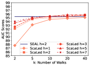
(a) AUC for USAir.

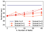
(b) Runtime for USAir.

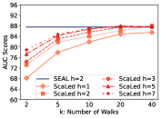
(c) AUC for Celegans.

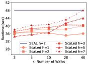
(d) Runtime for Celegans.

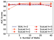
(e) AUC for NS.

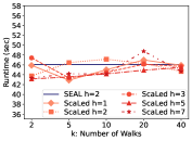
(f) Runtime for NS.

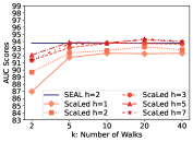
(g) AUC for Router.

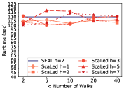
(h) Runtime for Router.

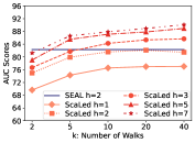
(i) AUC for Power.

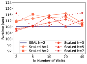
(j) Runtime for Power.

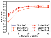
(k) AUC for Yeast.

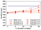
(l) Runtime for Yeast.

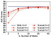
(m) AUC for Ecoli.

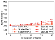
(n) Runtime for Ecoli.

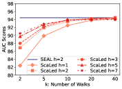
(o) AUC for PB.

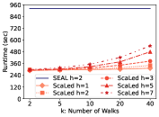
(p) Runtime for PB.

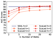
(q) AUC for Cora.

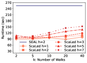
(r) Runtime for Cora.

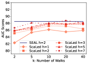
(s) AUC for CiteSeer.

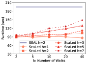
(t) Runtime for CiteSeer.

Figure 2. Average of AUCs and runtimes over 5 random seeds with various datasets, number of walks $k$, and walk lengh $h$.

Results: Hyperparameter Sensitivity Analyses. We intend to understand how the walk length $h$ and the number of walks $k$ control the computational overhead in ScaLed during training and inference. Thus, we conduct a sensitivity analysis of these two parameters on all of the attributed and non-attributed datasets. We vary $h$ and $k$ while keeping other hyperparameters fixed. Figure 2 reports the average AUC and runtime for all the datasets over 5 runs. The AUC results for all datasets are qualitatively similar where the AUC increases with both values of $h$ and $k$. One can also noticeably observe the runtime slightly increases with both walk length $h$ and the number of walks $k$ (with a few exceptions due to statistical noise). But, this slight increment of computational overhead elevates ScaLed’s accuracy measure and in the case of USAir, NS, Router, Power, Yeast and Cora pushes it towards and beyond that of SEAL. Interestingly, for datasets such as Ecoli and PB, when $k$ reaches $20$ and any $h$, the AUC of ScaLed gets very close to that of SEAL. We also observe that AUC increases much faster with the number of walks $k$ in comparison to the walk length $h$. For $h=2$ and $k=40$, ScaLed has outperformed or is comparable to SEAL in terms of AUC, but gained up to $3\times$ speed up, with the exceptions of NS, Router and Power where the runtime is similar to SEAL. The lack of speedup in those datasets might be explained by their low average degrees. Since these graphs are relatively sparse, the random walks discover the (close-to) exact enclosing subgraphs even with some potential redundancy by revisiting discovered nodes. Another interesting observation is that for large $h$ (e.g., $h=7$), ScaLed has not been able to outperform SEAL drastically. This observation confirms that a node’s local neighborhood has more information and we get diminishing returns by moving farther away from the target nodes. One practical conclusion is that for reaching high accuracy and maximum speed up, one is better off keeping the walk length $h$ low but increasing the number of walks $k$.

5. Conclusion and Future Works

Link prediction has emerged as an important task for graph-structured data with applications spanning across multiple domains. Existing state-of-the-art link predicion methods use subgraph representation learning (SGRL), which learns the enriched embedding of the enclosing subgraphs around the pair of nodes. However, SGRL methods are not scalable to large real-world graphs. We proposed ScaLed to overcome this scalability shortcomings, which exploits random walks to sample sparser enclosing subgraphs to reduce the computation overhead. The main idea is to preserve the key structural information of subgraphs with less number of nodes and edges, thus yielding smaller computational graphs for GNNs which in turn reduces the runtime and memory consumption. Our extensive experiments demonstrate ScaLed can match the accuracy measures of the state-of-the-art link prediction models while consuming order of magnitudes less resources. For future work, we plan to explore how to adaptively choose the length of the walks and the number of walks depending on the structural positions of two nodes. Another interesting research direction that could be explored is to apply graph augmentation techniques to the sampled subgraphs in ScaLed to further enhance its learning capabilities.

References

- (1)
- Adamic and Adar (2003) Lada A Adamic and Eytan Adar. 2003. Friends and Neighbors on the Web. Social Networks 25, 3 (2003), 211–230.
- Barabási and Albert (1999) Albert-László Barabási and Réka Albert. 1999. Emergence of Scaling in Random Networks. science 286, 5439 (1999), 509–512.
- Bevilacqua et al. (2022) Beatrice Bevilacqua, Fabrizio Frasca, Derek Lim, Balasubramaniam Srinivasan, Chen Cai, Gopinath Balamurugan, Michael M. Bronstein, and Haggai Maron. 2022. Equivariant Subgraph Aggregation Networks. In International Conference on Learning Representations.
- Brin and Page (2012) Sergey Brin and Lawrence Page. 2012. Reprint of: The anatomy of a large-scale hypertextual web search engine. Computer networks 56, 18 (2012), 3825–3833.
- Cai and Ji (2020) Lei Cai and Shuiwang Ji. 2020. A multi-scale approach for graph link prediction. In Proceedings of the AAAI Conference on Artificial Intelligence, Vol. 34. 3308–3315.
- Cai et al. (2021) Lei Cai, Jundong Li, Jie Wang, and Shuiwang Ji. 2021. Line Graph neural Networks for Link Prediction. IEEE Transactions on Pattern Analysis and Machine Intelligence (2021).
- Chen et al. (2018a) Jie Chen, Tengfei Ma, and Cao Xiao. 2018a. FastGCN: Fast Learning with Graph Convolutional Networks via Importance Sampling. In International Conference on Learning Representations.
- Chen et al. (2018b) Jianfei Chen, Jun Zhu, and Le Song. 2018b. Stochastic Training of Graph Convolutional Networks with Variance Reduction. In International Conference on Machine Learning. 942–950.
- Chen et al. (2020) Liang Chen, Yuanzhen Xie, Zibin Zheng, Huayou Zheng, and Jingdun Xie. 2020. Friend Recommendation based on Multi-social Graph Convolutional Network. IEEE Access 8 (2020), 43618–43629.
- Chiang et al. (2019) Wei-Lin Chiang, Xuanqing Liu, Si Si, Yang Li, Samy Bengio, and Cho-Jui Hsieh. 2019. Cluster-gcn: An Efficient Algorithm for Training Deep and Large Graph Convolutional Networks. In Proceedings of the 25th ACM SIGKDD International Conference on Knowledge Discovery & Data Mining. 257–266.
- Fey and Lenssen (2019) Matthias Fey and Jan E. Lenssen. 2019. Fast Graph Representation Learning with PyTorch Geometric. In ICLR Workshop on Representation Learning on Graphs and Manifolds.
- Fey et al. (2021) Matthias Fey, Jan E Lenssen, Frank Weichert, and Jure Leskovec. 2021. Gnnautoscale: Scalable and Expressive Graph Neural Networks via Historical Embeddings. In International Conference on Machine Learning. 3294–3304.
- Grover and Leskovec (2016) Aditya Grover and Jure Leskovec. 2016. node2vec: Scalable Feature Learning for Networks. In Proceedings of the 22nd ACM SIGKDD International Conference on Knowledge Discovery and Data Mining. 855–864.
- Gysi et al. (2021) Deisy Morselli Gysi, Ítalo Do Valle, Marinka Zitnik, Asher Ameli, Xiao Gan, Onur Varol, Susan Dina Ghiassian, JJ Patten, Robert A Davey, Joseph Loscalzo, et al. 2021. Network medicine framework for identifying drug-repurposing opportunities for COVID-19. Proceedings of the National Academy of Sciences 118, 19 (2021).
- Hamilton (2020) William L Hamilton. 2020. Graph representation learning. Synthesis Lectures on Artifical Intelligence and Machine Learning 14, 3 (2020), 1–159.
- Hamilton et al. (2017) William L Hamilton, Rex Ying, and Jure Leskovec. 2017. Inductive Representation Learning on Large Graphs. Advances in Neural Information Processing Systems 30 (2017).
- Hao et al. (2020) Yu Hao, Xin Cao, Yixiang Fang, Xike Xie, and Sibo Wang. 2020. Inductive Link Prediction for Nodes Having Only Attribute Information. In Proceedings of the Twenty-Ninth International Joint Conference on Artificial Intelligence, IJCAI-20. 1209–1215. https://doi.org/10.24963/ijcai.2020/168 Main track.
- Huang et al. (2020) Kexin Huang, Cao Xiao, Lucas M Glass, Marinka Zitnik, and Jimeng Sun. 2020. SkipGNN: predicting molecular interactions with skip-graph networks. Scientific reports 10, 1 (2020), 1–16.
- Katz (1953) Leo Katz. 1953. A New Status Index derived from Sociometric Analysis. Psychometrika 18, 1 (1953), 39–43.
- Kingma and Ba (2015) Diederik P. Kingma and Jimmy Ba. 2015. Adam: A Method for Stochastic Optimization. In International Conference on Learning Representations.
- Kipf and Welling (2016) Thomas N Kipf and Max Welling. 2016. Variational Graph Auto-Encoders. NIPS Workshop on Bayesian Deep Learning (2016).
- Kipf and Welling (2017) Thomas N. Kipf and Max Welling. 2017. Semi-Supervised Classification with Graph Convolutional Networks. In International Conference on Learning Representations.
- Koren et al. (2009) Yehuda Koren, Robert Bell, and Chris Volinsky. 2009. Matrix factorization techniques for recommender systems. Computer 42, 8 (2009), 30–37.
- Kumar et al. (2020) Ajay Kumar, Shashank Sheshar Singh, Kuldeep Singh, and Bhaskar Biswas. 2020. Link Prediction Techniques, Applications, and Performance: A Survey. Physica A: Statistical Mechanics and its Applications 553 (2020), 124289.
- Li et al. (2020) Pan Li, Yanbang Wang, Hongwei Wang, and Jure Leskovec. 2020. Distance Encoding: Design Provably More Powerful Neural Networks for Graph Representation Learning. Advances in Neural Information Processing Systems 33 (2020), 4465–4478.
- Liben-Nowell and Kleinberg (2007) David Liben-Nowell and Jon Kleinberg. 2007. The Link-prediction Problem for Social Networks. Journal of the American society for Information Science and Technology 58, 7 (2007), 1019–1031.
- Lü and Zhou (2011) Linyuan Lü and Tao Zhou. 2011. Link Prediction in Complex networks: A Survey. Physica A: statistical mechanics and its applications 390, 6 (2011), 1150–1170.
- Martínez et al. (2016) Víctor Martínez, Fernando Berzal, and Juan-Carlos Cubero. 2016. A Survey of Link Prediction in Complex Networks. ACM Computing Surveys (CSUR) 49, 4 (2016), 1–33.
- Page et al. (1999) Lawrence Page, Sergey Brin, Rajeev Motwani, and Terry Winograd. 1999. The PageRank citation ranking: Bringing order to the web. Technical Report. Stanford InfoLab.
- Pan et al. (2022) Liming Pan, Cheng Shi, and Ivan Dokmanić. 2022. Neural Link Prediction with Walk Pooling. In International Conference on Learning Representations.
- Paszke et al. (2019) Adam Paszke, Sam Gross, Francisco Massa, Adam Lerer, James Bradbury, Gregory Chanan, Trevor Killeen, Zeming Lin, Natalia Gimelshein, Luca Antiga, et al. 2019. Pytorch: An imperative style, high-performance deep learning library. Advances in Neural Information Processing Systems 32 (2019).
- Perozzi et al. (2014) Bryan Perozzi, Rami Al-Rfou, and Steven Skiena. 2014. Deepwalk: Online Learning of Social Representations. In Proceedings of the 20th ACM SIGKDD International Conference on Knowledge Discovery and Data Mining. 701–710.
- Veličković et al. (2018) Petar Veličković, Guillem Cucurull, Arantxa Casanova, Adriana Romero, Pietro Liò, and Yoshua Bengio. 2018. Graph Attention Networks. International Conference on Learning Representations (2018).
- Wang et al. (2022) Haorui Wang, Haoteng Yin, Muhan Zhang, and Pan Li. 2022. Equivariant and Stable Positional Encoding for More Powerful Graph Neural Networks. In International Conference on Learning Representations.
- Wang et al. (2015) Peng Wang, BaoWen Xu, YuRong Wu, and XiaoYu Zhou. 2015. Link Prediction in Social Networks: the state-of-the-art. Science China Information Sciences 58, 1 (2015), 1–38.
- Wu et al. (2020) Zonghan Wu, Shirui Pan, Fengwen Chen, Guodong Long, Chengqi Zhang, and S Yu Philip. 2020. A comprehensive survey on graph neural networks. IEEE Transactions on Neural Networks and Learning Systems 32, 1 (2020), 4–24.
- Xu et al. (2019) Keyulu Xu, Weihua Hu, Jure Leskovec, and Stefanie Jegelka. 2019. How Powerful are Graph Neural Networks?. In International Conference on Learning Representations.
- Yin et al. (2022) Haoteng Yin, Muhan Zhang, Yanbang Wang, Jianguo Wang, and Pan Li. 2022. Algorithm and System Co-design for Efficient Subgraph-based Graph Representation Learning. arXiv preprint arXiv:2202.13538 (2022).
- Ying et al. (2018) Rex Ying, Ruining He, Kaifeng Chen, Pong Eksombatchai, William L Hamilton, and Jure Leskovec. 2018. Graph Convolutional Neural Networks for Web-scale Recommender Systems. In Proceedings of the 24th ACM SIGKDD International Conference on Knowledge Discovery & Data Mining. 974–983.
- You et al. (2021) Jiaxuan You, Jonathan M. Gomes-Selman, Rex Ying, and Jure Leskovec. 2021. Identity-aware Graph Neural Networks. In Proceedings of the AAAI Conference on Artificial Intelligence.
- You et al. (2019) Jiaxuan You, Rex Ying, and Jure Leskovec. 2019. Position-aware Graph Neural Networks. In International Conference on Machine Learning. 7134–7143.
- Zeng et al. (2021) Hanqing Zeng, Muhan Zhang, Yinglong Xia, Ajitesh Srivastava, Andrey Malevich, Rajgopal Kannan, Viktor Prasanna, Long Jin, and Ren Chen. 2021. Decoupling the Depth and Scope of Graph Neural Networks. Advances in Neural Information Processing Systems 34 (2021).
- Zeng et al. (2020) Hanqing Zeng, Hongkuan Zhou, Ajitesh Srivastava, Rajgopal Kannan, and Viktor Prasanna. 2020. GraphSAINT: Graph Sampling Based Inductive Learning Method. In International Conference on Learning Representations.
- Zhang and Chen (2017) Muhan Zhang and Yixin Chen. 2017. Weisfeiler-Lehman Neural Machine for Link Prediction. In Proceedings of the 23rd ACM SIGKDD International Conference on Knowledge Discovery and Data Mining. 575–583.
- Zhang and Chen (2018) Muhan Zhang and Yixin Chen. 2018. Link Prediction based on Graph Neural Networks. Advances in Neural Information Processing Systems 31 (2018).
- Zhang et al. (2018) Muhan Zhang, Zhicheng Cui, Marion Neumann, and Yixin Chen. 2018. An End-to-end Deep Learning Architecture for Graph Classification. In Proceedings of the AAAI Conference on Artificial Intelligence.
- Zhang et al. (2021) Muhan Zhang, Pan Li, Yinglong Xia, Kai Wang, and Long Jin. 2021. Labeling Trick: A Theory of Using Graph Neural Networks for Multi-Node Representation Learning. Advances in Neural Information Processing Systems 34 (2021).
- Zhou et al. (2020) Jie Zhou, Ganqu Cui, Shengding Hu, Zhengyan Zhang, Cheng Yang, Zhiyuan Liu, Lifeng Wang, Changcheng Li, and Maosong Sun. 2020. Graph Neural Networks: A Review of Methods and Applications. AI Open 1 (2020), 57–81.
- Zou et al. (2019) Difan Zou, Ziniu Hu, Yewen Wang, Song Jiang, Yizhou Sun, and Quanquan Gu. 2019. Layer-dependent Importance Sampling for Training Deep and Large Graph Convolutional Networks. Advances in Neural Information Processing Systems 32 (2019).