Affinity-Aware Graph Networks

Abstract

Graph Neural Networks (GNNs) have emerged as a powerful technique for learning on relational data. Owing to the relatively limited number of message passing steps they perform—and hence a smaller receptive field—there has been significant interest in improving their expressivity by incorporating structural aspects of the underlying graph. In this paper, we explore the use of affinity measures as features in graph neural networks, in particular measures arising from random walks, including effective resistance, hitting and commute times. We propose message passing networks based on these features and evaluate their performance on a variety of node and graph property prediction tasks. Our architecture has lower computational complexity, while our features are invariant to the permutations of the underlying graph. The measures we compute allow the network to exploit the connectivity properties of the graph, thereby allowing us to outperform relevant benchmarks for a wide variety of tasks, often with significantly fewer message passing steps. On one of the largest publicly available graph regression datasets, OGB-LSC-PCQM4Mv1, we obtain the best known single-model validation MAE at the time of writing.

1 Introduction

Graph Neural Networks (GNNs) constitute a powerful tool for learning meaningful representations in non-Euclidean domains. GNN models have achieved significant successes in a wide variety of node prediction [18, 28], link prediction [49, 47], and graph prediction [11, 45] tasks. These tasks naturally emerge in a wide range of applications, including autonomous driving [8], neuroimaging [32], combinatorial optimization [14, 31], and recommender systems [46], while they have enabled significant scientific advances in the fields of biomedicine [40], structural biology [22], molecular chemistry [37] and physics [3].

Despite the predictive power of GNNs, it is known that the expressive power of standard GNNs is limited by the 1-Weisfeiler-Lehman (1-WL) test [42]. Intuitively, GNNs possess the same power in terms of distinguishing between non-isomorphic (sub-)graphs, while having the added benefit of adapting to the given data distribution. For some architectures, two nodes with different local structures have the same computational graph, thus thwarting distinguishability in a standard GNN. Even though some attempts have been made to address this limitation with higher-order GNNs [29], most traditional GNN architectures fail to distinguish between such nodes.

Contributions: We propose the use of affinity metrics as features in a graph neural network to circumvent this limitation. Specifically, we consider statistics that arise from random walks in graphs, such as hitting time and commute time between pairs of vertices. We present a means of incorporating these statistics as scalar edge features in a message passing neural network (MPNN) [15]. Additionally, we present a set of vector-valued resistive embeddings that can be incorporated as node or edge feature vectors in the network. We show that such embeddings can be efficiently approximated, even for larger graphs, using sketching and dimensionality reduction techniques.

Moreover, we evaluate our networks on a number of benchmark datasets of diverse scales. First, we show that our networks outperform other baselines on the PNA dataset [9], which includes 6 node and graph algorithmic tasks, showing the ability of affinity measures to exploit structural properties of graphs. We also evaluate the performance on a number of graph and node tasks for datasets in the Open Graph Benchmark (OGB) collection [20], including molecular and citation graphs. In particular, our networks with scalar effective resistance edge features achieve the state of the art on the OGB-LSC PCQM4Mv1 dataset, which was featured in a KDD Cup 2021 competition for large scale graph representation learning.

2 Related Work

Our work builds upon a wealth of graph theoretical and graph representation learning works, while we focus on a supervised, inductive setting.

Even though GNN architectures were originally classified as spectral or spatial, we abstain from this division as recent research has demonstrated some equivalence of the graph convolution process regardless of the choice of convolution kernels [2, 7]. Spectrally-motivated methods require the eigendecomposition of the graph Laplacian matrix (or an approximation thereof) and, hence, corresponding convolutions capture different frequencies of the graph signal. Early works in this space include ChebNet [10] and the more efficient kernel reparametrisation by Kipf et al. [23] to which we compare our work. Levie et al. [25] proposed CayleyNets, an alternative polynomial approximation of the Laplacian eigendecomposition.

Message passing neural networks (MPNNs) [15] perform a transformation of node and edge representations before and after an arbitrary aggregator (e.g. sum). Graph attention networks (GATs) [39] aimed to improve the expressivity of GNNs by allowing graph nodes to “attend” differently to different edges inspired by the success of transformers in NLP tasks. One of the most relevant works was proposed by Beaini et al. [4], i.e. directional graph networks (DGN). DGN uses the gradients of the low-frequency eigenvectors of the graph Laplacian, which are known to capture key information about the global structure of the graph and prove that the aggregators they construct using these gradients lead to more discriminative models than standard GNNs according to the 1-WL test. Prior work [29] used higher-order ($k$-dimensional) GNNs, based on $k$-WL, and a hierarchical variant and proved theoretically and experimentally the improved expressivity in comparison to other models.

Other notable works include Position-aware Graph Neural Networks [47] that capture positions/locations of nodes with respect to a set of anchor nodes, Distance Encoding Networks [26] that use the first few powers of the normalized adjacency matrix as node features, and Graph Isomoprhism Networks (GINs) [42]. Hamilton et al. [18] proposed a method to constuct node representations by sampling a fixed-size neighborhood of each node, and then performing a specific aggregator over it, which led to impressive performance on large-scale inductive benchmarks. Bouritsas et al. [6] use topologically-aware message passing to detect and count graph substructures, while Bornar et al. [5] propose a message-passing procedure on cell complexes motivated by a novel colour refinement algorithm to test their isomorphism which prove to be powerful for molecular benchmarks.

3 Affinity Measures and GNNs

Our goal is to incorporate affinity measures related to random walk metrics on graphs into the GNN architecture.

3.1 Random Walks, Hitting and Commute Times

We define several natural properties of a graph that arise from a random walk. A random walk on $G$ starting from a node $u$ is a Markov chain on the vertex set $V$ such that the initial vertex is $u$, and at each time step, one moves from the current vertex to a neighbor, chosen with probability proportional to the weight of outgoing edges. We will use $\pi$ to denote the stationary distribution of this Markov Chain. For random walks on weighted, undirected graphs, we know that $\pi_{u}=\frac{d_{u}}{2M}$, where $d_{u}$ is the weighted degree of node $u$, and $M$ is the sum of edge weights.

The hitting time $H_{uv}$ fom $u$ to $v$ is defined as the expected number of steps for a random walk starting at $u$ to hit $v$. We can also define the commute time between $u$ and $v$ as $K_{uv}=H_{uv}+H_{vu}$, the expected round-trip time for a random walk starting at $u$ to reach $v$ and then return to $u$.

3.2 Effective Resistance

A closely related quantity is the measure of effective resistances in undirected graphs. This quantity corresponds to the effective resistance if the whole graph was replaced with a circuit where each edge becomes a resistor with resistance equal to the reciprocal of its weight. We will use $\mathsf{Res}(u,v)$ to denote the effective resistance between nodes $u$ and $v$. For undirected graphs, it is known that [27] the effective resistance is proportional to the commute time, $\mathsf{Res}(u,v)=\frac{1}{2M}K_{uv}.$

In light of the above, our broad goal is to incorporate effective resistances and hitting times as edge features in an MPNN, as we describe in Section 3.4.

3.3 Resistive Embeddings

Effective resistances allow us to define the resistive embedding, a mapping that associates each node $v$ of a graph $G=(V,E,W)$, where $W$ are the non-negative edge weights, with an embedding vector. Before we specify the resistive embedding, we define a few terms. Let $L=D-A$ be the graph Laplacian of $G$, where $D\in\mathbb{R}^{n\times n}$ is the diagonal matrix containing the weighted degree of each node and $A\in\mathbb{R}^{n\times n}$ is the adjacency matrix, whose $(i,j)^{th}$ entry is equal to the edge weight between $i$ and $j$, if exists; and $0$ otherwise. Let $B$ be the $m\times n$ edge-node incidence matrix, where $|V|=n$ and $|E|=m$, defined as follows: The $i$-th row of $B$ corresponds to the $i$-th edge $e_{i}=(u_{i},v_{i})$ of $G$ and has a $+1$ in the $u_{i}$-th column and a $-1$ in the $v_{i}$-th column, while all other entries are zero. Finally we will use $C\in\mathbb{R}^{m\times m}$ to denote the conductance matrix, which is a diagonal matrix with $C_{ii}$ being the weight of $i^{th}$ edge. It is easy to verify that $B^{T}CB=L$. Even though $L$ is not invertible, its null-space consists of the indicator vectors for every connected component of $G$. For example, if $G$ is connected, then $L$’s nullspace consists only of the multiples of all-$1$’s vector . Hence, for any vector $x$ orthogonal to all-$1$’s, $L\cdot L^{\dagger}x=x$, where $L^{\dagger}$ is the pseudo-inverse.

We can express effective resistance between any pair of nodes using Laplacian matrices [27] as $\mathsf{Res}(u,v)=(\mathbf{1}_{u}-\mathbf{1}_{v})^{T}L^{\dagger}(\mathbf{1}_{u}-\mathbf{1}_{v}),$ where $\mathbf{1}_{v}$ is an $n$-dimensional vector specifying the indicator for node $v$. We are now ready to define the resistive embedding.

Definition 3.1.

(Effective Resistance Embedding) $\mathbf{r}_{v}=C^{1/2}BL^{\dagger}\mathbf{1}_{v}.$

The useful property for us is that the effective resistance between two nodes in the graph can be obtained easily from the distance between their corresponding embedding.

Lemma 3.2.

For any pair of nodes $u,v$, we have $\|\mathbf{r}_{u}-\mathbf{r}_{v}\|_{2}^{2}=\mathsf{Res}(u,v)$.

The proof of this lemma can be found in Appendix B. One can easily check that any rotation of $\mathbf{r}$ also satisfies Lemma 3.2, since rotations preserve Euclidean distances. In particular, if $U$ is an orthonormal matrix, then $U\mathbf{r}$ is also a valid resistive embedding. In other words, resistive embeddings are unique with respect to rotations. This poses a challenge if we want to use the resistive embeddings as node or edge features: we need a way to enforce that a (G)NN using them will do so in a way that is invariant or equivariant to any rotations of the embeddings. In our current work, we rely on data augmentation: at every training iteration, we apply random rotations to the input ER embeddings.

Remark 3.3.

While data augmentation is a popular approach for promoting invariant and equivariant predictions, it is only hinting to the network that such predictions are favourable. It is also possible, in the spirit of the geometric deep learning blueprint [7], to combine ER embeddings with an $O(n)$-equivariant GNN, which rigorously enforces rotational equivariance. A popular approach to building equivariant GNNs has been proposed by  [35], though it focuses on the full Euclidean group $E(n)$ rather than $O(n)$. We leave this exploration to future work.

Definition 3.4.

Let $\mathbf{p}:=\sum_{u}\pi_{u}\mathbf{r}_{u}$ be the mean of effective resistance embedding.

We might view $\mathbf{p}$ as a “weighted mean” of $\mathbf{r}$. We will define the hitting time radius, $H_{\max}$, of a given graph as the maximum hitting time between any two nodes:

Definition 3.5 (Hitting Time Radius).

$H_{\max}:=\max_{u,v}H_{u,v}$.

We will need the following to bound the hitting times we computed:

Lemma 3.6.

For any node $u$, $\|\mathbf{r}_{u}-\mathbf{p}\|^{2}\leq\frac{H_{\max}}{M}$.

The proof of Lemma 3.6 follows immediately from the fact that $\mathbf{p}$ is a convex combination of all $\mathbf{r}$’s and Jensen’s inequality.

3.4 Incorporating Features into MPNNs

We reiterate that our main aim is to demonstrate (theoretically and empirically) that there are good reasons to incorporate affinity-based measures into GNN computations.

In the simplest instance, a method that improves a GNN’s expressive power may compute additional features (positional or structural) which would assist the GNN in discriminating between examples it otherwise wouldn’t (easily) be able to. These features are then appended to the GNN’s inputs for further processing. For example, it has been shown that endowing nodes with a one-hot based identity is already sufficient for improving expressive power [30]; this was then relaxed to any randomly-sampled scalar feature by Sato et al. [34]. It is, of course, possible to create dedicated features that even count substructures of interest [6]. Further, the adjacency information can be factorised [33] or eigendecomposed [12] to provide useful structural embeddings for the GNN.

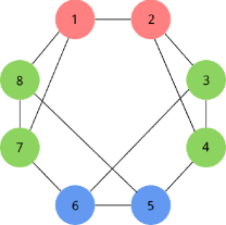
Figure 1: Degree 3 graph on 8 nodes, with isomorphism classes indicated by colors. While nodes of the same color are structurally identical, nodes of different colors are not. A standard GNN limited by the 1-WL cannot distinguish between nodes of different colors. However, affinity based networks that use effective resistances, hitting times, or resistive embeddings can distinguish every pair of such nodes.

We will focus our attention on exactly this class of methods, as it is a lightweight and direct way of demonstrating improvements from these computations. Hence, our baselines will all be instances of the MPNN framework [15], which we will attempt to improve by endowing them with affinity-based features. We start by theoretically proving that these features indeed improve expressive power:

Theorem 3.7.

MPNNs that make use of any one of (a) effective resistances, (b) hitting times, (c) resistive embeddings are strictly more powerful than the WL-1 test.

Proof.

Since the networks in question arise from augmenting standard MPNNs with additional node/edge features, we have that these networks are at least as powerful as the 1-WL test.

In order to show that these networks are strictly more powerful than the 1-WL test, it suffices to show the existence of a graph for which our affinity measure based networks can distinguish between certain nodes that a standard GNN (limited by the 1-WL test) cannot.

We present an example of a 3-regular graph (see Figure 1) on 8 nodes. It is well-known that a standard GNN that is limited by the 1-WL test cannot distinguish any pair of nodes in a regular graph, as the computation tree rooted at any node in the graph looks identical. However, there are three isomorphism classes of nodes in the above graph (denoted by different colors), namely, $V_{1}=\{1,2\}$, $V_{2}=\{3,4,7,8\}$, and $V_{3}=\{5,6\}$.

We now show that GNNs with affinity based measures can distinguish between a node in $V_{i}$ and a node in $V_{j}$, for $i\neq j$. We note that the hitting time from $a$ to $b$ depends only on the isomorphism classes of $a$ and $b$. Thus, we write $r_{i,j}$ as the effective resistance between a node in $V_{i}$ and a node in $V_{j}$. Note that $r_{i,j}=r_{j,i}$, and it is easy to verify that $r_{1,1}=2/3,r_{2,2}=15/28,r_{3,3}=4/7,r_{1,2}=r_{2,1}=185/336,r_{2,3}=r_{3,2}=209/336.$ Hence, it follows that in a message passing step of an MPNN that uses effective resistances, vertices in $V_{1}$, $V_{2}$, and $V_{3}$ will aggregate feature multisets $\{r_{1,1},r_{1,2},r_{1,2}\}=\{2/3,185/336,185/336\}$, $\{r_{2,1},r_{2,2},r_{2,3}\}=\{185/336,15/28,209/336\}$, and $\{r_{2,3},r_{2,3},r_{3,3}\}=\{209/336,209/336,4/7\}$, respectively, all of which are all distinct multisets. Hence, such an MPNN can distinguish nodes in $V_{i}$ and $V_{j}$, $i\neq j$ for a suitable aggregation function.

Note that if instead of scalar effective resistance features, an MPNN uses hitting time features or resistive embeddings, it can distinguish the same isomorphism classes as above because the effective resistance between nodes is a function of the two hitting times in either direction as well as of the resistive embeddings of the two nodes (see lemma 3.2). In other words, one can reduce to the case of scalar effective resistance features by composing the aggregation function with the appropriate function that transforms either hitting times or resistive embeddings to effective resistances. ∎

We also compare our method to other strong feature-based approaches in the literature. The recently proposed DE-GNNs [26] are arguably one of the closest proposals to ours, as they compute distance-encoded features. These features can be at least as powerful as our proposed affinity-based features if polynomially many powers of the adjacency matrix are used. However, for all but the smallest graphs, using this many powers will be impractical—in fact, [26] only use powers of $A$ up to 3, which would not be able to reliably approximate affinity-based features.

Ultimately, a technique that improves a GNN’s expressive power can do so in three broad directions. While we focus on the feature-based direction in this paper, we also acknowledge that it in no way compels the GNN to use the additional provided features. Hence, we briefly survey the other two, as an indication of the future research in affinity-based GNNs we hope this work will inspire.

One avenue involves modulating the message passing rule to make advantage of the desired computations. Popular recent examples of this include DGN [4] and LSPE [12]. DGNs leverage the graph’s Laplacian eigenvectors, but they do not merely use them as input features; instead, they define a directional vector field based on the eigenvectors, and use it explicitly to anisotropically aggregate neighbourhoods. LSPE features a “bespoke pipeline” for processing positional inputs.

The other direction is to modulate the graph over which messages are passed, usually by adding new nodes that correspond to desired substructures. An early proponent of this is the work of [29], which explicitly performs message passing over $k$-tuples of nodes at once. Recently, scalable efforts in this direction focus on carefully chosen substructures, e.g., junction trees [13], cellular complexes [5].

3.5 Effective Resistance vs. Shortest Path Distance

It is interesting to compare the use of effective resistances with shortest path distances (SPDs) in GNNs, given the considerable number of recent works that make use of SPDs (e.g., Graphormer [44], Position-Aware GNN [47], DE-GNN [26]). The most direct comparison of our effective resistance-based MPNNs would be to use SPDs as edge features in the MPNNs. However, note that SPDs along graph edges are a trivial feature (unlike effective resistances, which still incorporate useful information about the global graph structure).

An alternative to edge features would be to use (a) SPDs to a small set of anchor nodes as features in an MPNN (e.g., P-GNN [47]) or (b) a dense featurization incorporating shortest paths between all pairs of nodes (e.g., the dense attention mechanism in Graphormer [44]). We remark that the latter approach typically incurs an $O(n^{2})$ overhead, which our MPNN-based approach avoids.

We empirically compare our models to MPNNs that use approaches (a) and (b). Results on the PNA dataset show that our effective resistance-based GNNs outperform these approaches. Furthermore, we complement these empirical results with a theoretical result showing that under a limited number of message-passing steps, effective resistance features can allow one to distinguish structures that cannot be done using shortest path features. We point the reader to the appendix for these results.

4 Efficient Computation of Affinity Measures

In order to use our features, it is important that they be computable efficiently. In this section, we show how to compute or approximate the various random walk-based affinity measures.

4.1 Reducing Dimensionality of Resistive Embeddings

For each edge, we seek to use the resistive embeddings as GNN features instead of the effective resistance. Now, the difficulty with using resistive embeddings directly as GNN features is the fact that the embeddings have dimension $m$, which can be quite large, e.g., up to $n^{2}$ for dense graphs. It was shown by [36] that one can reduce the dimensionality of the embedding while approximately preserving Euclidean distances. The idea is to use a random projection via a constructive version of the Johnson-Lindenstrauss Lemma:

Lemma 4.1 (Constructive Johnson-Lindenstrauss).

Let $x_{1},x_{2},\ldots,x_{n}\in\mathbb{R}^{d}$ be a set of $n$ points; and let $\alpha_{1},\alpha_{2},\ldots,\alpha_{m}\in\mathbb{R}^{n}$ be fixed linear combinations. Suppose $\Pi$ is a $k\times d$ matrix whose entries are chosen i.i.d. from a Gaussian $N(0,1)$ and consider $\widehat{x_{i}}:=\frac{1}{\sqrt{k}}\Pi x_{i}$.

Then, it follows that for $k\geq C\log(mn)/\epsilon^{2}$, with probability $1-o(1)$, we have $\|\sum_{j}\alpha_{i,j}\widehat{x}_{j}\|^{2}=(1\pm\epsilon)\|\sum_{j}\alpha_{i,j}x_{j}\|_{2}^{2}$ for every $1\leq j\leq m$.

Using triangle inequality, we can see that the inner products between fixed linear combinations are preserved up to some additive error:

Corollary 4.2.

For any fixed vectors $\alpha,\beta\in\mathbb{R}^{n}$, if we let $X:=\sum_{i}\alpha_{i}{x}_{i}$, $\widehat{X}:=\sum_{i}\alpha_{i}\widehat{x}_{i}$ and similarly $Y:=\sum_{i}\beta_{i}{x}_{i}$, $\widehat{Y}:=\sum_{i}\beta_{i}\widehat{x}_{i}$; then $\left|\langle X,Y\rangle-\langle\widehat{X},\widehat{Y}\rangle\right|\leq\frac{\epsilon}{2}\left(\|X\|^{2}+\|Y\|^{2}\right).$

The proof of Corollary 4.2 can be found in Appendix B.

Therefore, we can choose a desired $\epsilon>0$ and $k=O(\log(n)/\epsilon^{2})$ and instead use $\mathbf{\widehat{r}}:V\to\mathbb{R}^{k}$ as the embedding, where $\mathbf{\widehat{r}}_{v}=\frac{1}{\sqrt{k}}\Pi BL^{\dagger}e_{v}$ for a randomly chosen $k\times d$ matrix $\Pi$ whose entries are i.i.d. Gaussians from $\mathcal{N}(0,1)$. Then, by Lemma 3.2 and Lemma 4.1, we have that for every edge $(u,v)\in E$, $\|\mathbf{\widehat{r}}_{u}-\mathbf{\widehat{r}}_{v}\|_{2}^{2}=(1\pm 3\epsilon)\mathsf{Res}(u,v)$ with probability at least $1-\frac{1}{n^{2}}$.

So the computation of random embeddings, $\mathbf{\widehat{r}}$, requires solving $O((n+m)\log n/\epsilon^{2})$ many Laplacian linear systems. By using one of the fast Laplacian solvers [24], we can compute the random embeddings in the near-linear time. Hence the total running time becomes $\widetilde{O}(n+m)$.

4.2 Fast Computation of Hitting Times

Note that it is not clear how to compute hitting times efficiently as in the case of commute times / effective resistances. The naive approach involves solving a linear system for each edge, resulting in a running time of $\Omega(nm)$, which is prohibitive. One of our technical contributions in this paper is a method for fast computation of hitting times. In particular, we will show how to use the approximate effective resistance embeddings, $\mathbf{\widehat{r}}$, to obtain an estimate for hitting times with additive error.

Let $\widehat{\mathbf{p}}:=\sum_{u}\pi_{u}\mathbf{\widehat{r}}_{u}$. Just like $\mathbf{\widehat{r}}$ being an approximation of $\mathbf{r}$, $\widehat{\mathbf{p}}$ is an approximation of $\mathbf{p}$. Consider the following quantity, $\widehat{H}_{u,v}=2M\langle\mathbf{\widehat{r}}_{v}-\mathbf{\widehat{r}}_{u},\mathbf{\widehat{r}}_{v}-\widehat{\mathbf{p}}\rangle$. We will use this quantity as an approximation of $H_{u,v}$. In the following part, we will bound the difference between $H_{u,v}$ and $\widehat{H}_{u,v}$. Our starting point will be expressing $H_{u,v}$ in terms of the effective resistance embeddings.

Lemma 4.3.

${H}_{u,v}=2M\langle\mathbf{r}_{v}-\mathbf{r}_{u},\mathbf{r}_{v}-{\mathbf{p}}\rangle$ where $\mathbf{p}:=\sum_{u}\pi_{u}\mathbf{r}_{u}$.

The proof of Lemma 4.3 can be found in Appendix B.

Theorem 4.4.

$|\widehat{H}_{u,v}-H_{u,v}|\leq 3\epsilon H_{\max}$.

Proof.

Using Lemma 4.3, we see that $|\widehat{H}_{u,v}-H_{u,v}|$ can be bounded as

$$2M\left|\langle\mathbf{\widehat{r}}_{v}-\mathbf{\widehat{r}}_{u},\mathbf{\widehat{r}}_{v}-\widehat{\mathbf{p}}\rangle-\langle\mathbf{r}_{v}-\mathbf{r}_{u},\mathbf{r}_{v}-\mathbf{p}\rangle\right|\leq\epsilon M\left(\|\mathbf{r}_{v}-\mathbf{r}_{u}\|^{2}+\|\mathbf{r}_{v}-\mathbf{p}\|^{2}\right)\leq 3\epsilon H_{\max},$$

where we used Corollary 4.2 in the first inequality and Definition 3.5 in the last inequality. ∎

5 Experiments

5.1 Baselines

As previously discussed, our empirical evaluation seeks to show benefits from endowing standard expressive GNNs with additional affinity-based features. All architectures we experiment with will therefore conform to the message passing neural network (MPNN) blueprint [15], which we now briefly describe for convenience.

Assume that our input graph, $\mathcal{G}=(\mathcal{V},\mathcal{E})$, has node features $\mathbf{x}_{u}\in\mathbb{R}^{n}$, edge features $\mathbf{x}_{uv}\in\mathbb{R}^{m}$ and graph-level features $\mathbf{x}_{\mathcal{G}}\in\mathbb{R}^{l}$, for nodes $u,v\in\mathcal{V}$ and edges $(u,v)\in\mathcal{E}$. We provide encoders $f_{n}:\mathbb{R}^{n}\rightarrow\mathbb{R}^{k}$, $f_{e}:\mathbb{R}^{m}\rightarrow\mathbb{R}^{k}$ and $f_{g}:\mathbb{R}^{l}\rightarrow\mathbb{R}^{k}$ that transform these inputs into a latent space:

$$\mathbf{h}_{u}^{(0)}=f_{n}(\mathbf{x}_{u})\qquad\mathbf{h}_{uv}^{(0)}=f_{e}(\mathbf{x}_{uv})\qquad\mathbf{h}_{\mathcal{G}}^{(0)}=f_{g}(\mathbf{x}_{\mathcal{G}})$$ (1)

Our MPNN then performs several message passing steps $\mathbf{H}^{(t+1)}=P_{t+1}(\mathbf{H}^{(t)})$ where $\mathbf{H}^{(t)}=\Big{(}\big{\{}\mathbf{h}_{u}^{(t)}\big{\}}_{u\in\mathcal{V}},\big{\{}\mathbf{h}_{uv}^{(t)}\big{\}}_{(u,v)\in\mathcal{E}},\mathbf{h}_{\mathcal{G}}^{(t)}\Big{)}$ contains all of the latents at a particular processing step $t\geq 0$.

This process is iterated for $T$ steps, recovering final latents $\mathbf{H}^{(T)}$. These can then be decoded into node-, edge-, and graph-level predictions (as required), using analogous decoder functions $g_{n}$, $g_{e}$, $g_{g}$:

$$\mathbf{y}_{u}=g_{n}(\mathbf{h}_{u}^{(T)}),\qquad\mathbf{y}_{uv}=g_{e}(\mathbf{h}_{uv}^{(T)}),\qquad\mathbf{y}_{\mathcal{G}}=g_{g}(\mathbf{h}_{\mathcal{G}}^{(T)})$$ (2)

Generally, $f$, $g$ are MLPs, while we use an MPNN update rule for $P$. It computes message vectors, $\mathbf{m}^{(t)}_{uv}$, to be sent across the edge $(u,v)$ and then aggregates them at the receiver nodes as follows:

$$\mathbf{m}^{(t+1)}_{uv}=\psi_{t+1}\big{(}\mathbf{h}^{(t)}_{u},\mathbf{h}^{(t)}_{v},\mathbf{h}^{(0)}_{uv}\big{)};\quad\mathbf{h}^{(t+1)}_{u}=\phi_{t+1}\Big{(}\mathbf{h}^{(t)}_{u},\sum_{u\in\mathcal{N}_{v}}\mathbf{m}^{(t+1)}_{vu}\Big{)}.$$ (3)

The message function $\psi_{t+1}$ and the update function $\phi_{t+1}$ are both MLPs. All of our models have been implemented using the Jraph library [16].

Occasionally, the dataset in question will be easy to overfit with the most general form of message function (eq. 3). In these cases, we resort to assuming that $\psi$ factorises into an attention mechanism $\mathbf{m}^{(t+1)}_{uv}=a_{t+1}\big{(}\mathbf{h}^{(t)}_{u},\mathbf{h}^{(t)}_{v},\mathbf{h}^{(0)}_{uv}\big{)}\psi_{t+1}\big{(}\mathbf{h}^{(t)}_{u}\big{)}$, where the attention function $a$ is scalar-valued. We will refer to this particular MPNN baseline as a graph attention network (GAT) [39].

When relevant, we may also recall the results that a particular strong baseline (such as DGN [4] or Graphormer [43]) achieves on a dataset of interest. Note that these baselines modulate the message passing procedure rather than appending features, and are, hence, a different category to our method—their performance is provided for indicative reasons only. Where appropriate, we will use “DGN (features)” to refer to an MPNN that uses the eigenvector flows as additional edge features, without modulating the mechanism.

		Node tasks			Graph tasks
Model	Avg score	SSSP	Ecc	Lap feat	Conn	Diam	Spec rad
GAT	-1.730	-2.213	-1.935	-2.644	-0.618	-1.430	-1.538
GCN	-1.592	-2.283	-1.978	-1.698	-0.618	-1.432	-1.541
MPNN	-2.665	-2.235	-2.419	-3.116	-1.887	-2.681	-3.652
MPNN (rand features)	-2.490	-2.136	-1.808	-3.873	-1.696	-2.614	-2.813
DGN (features)	-2.743	-2.165	-1.911	-4.184	-1.858	-2.814	-3.528
ER GNN	-2.779	-2.146	-1.869	-3.945	-1.962	-2.940	-3.811
ER (node) embeddings	-2.658	-2.245	-2.493	-3.533	-1.649	-2.886	-3.144
ER (edge) embeddings	-2.789	-2.266	-2.125	-4.253	-1.664	-2.807	-3.617
Hitting Times	-2.816	-2.189	-1.904	-4.397	-1.888	-2.796	-3.720
All ER features	-3.106	-2.789	-3.082	-4.047	-1.858	-2.894	-3.962

Table 1: $log(MSE)$ on the PNA test dataset

5.2 Datasets

5.2.1 PNA dataset

The first dataset we explore is the PNA dataset [9], which captures a multimodal setting. This consists of a collection of node tasks, i.e., (1) Single-source shortest paths, (2) Eccentricity and (3) Laplacian features, as well as graph tasks, i.e. (4) Connectivity, (5) Diameter and (6) Spectral radius. PNA is a set of structured tasks that complements our other datasets. Our results are given in Table 1.

As we can see from the table, even adding a single feature, effective resistance (ER GNN), yields the best average score compared to other models. As expected using hitting times as edge features improve upon effective resistances. However once we combine all ER features, which include effective resistances, hitting times as well as node and edge embeddings, we get the best scores. On these structured tasks, we can see that the affinity based measures provide a significant advantage.

	MolHIV Test % ROC-AUC
GCN	$76.06\pm 0.97$
MPNN	$74.67\pm 0.19$
MPNN + Random Features	$75.52\pm 1.07$
DGN	$\textbf{79.70}\pm 0.97$
ER GNN	$77.75\pm 0.426$
Hitting Times	$76.56\pm 0.915$
ER (node) embeddings	$77.77\pm 0.339$
ER (edge) embeddings	$76.18\pm 0.992$
ER (node) embeddings + HT	$78.16\pm 0.792$
ER (node) embeddings (with random rotations)	$76.28\pm 0.541$
ER (node) embeddings + HT (with random rotations)	$\textit{79.13}\pm 0.358$

Table 2: Test % AUC-ROC averaged over 5 seeds.

5.2.2 Small molecule classification: ogbg-molhiv

The ogbg-molhiv dataset is a molecular property prediction dataset comprised of molecular graphs without spatial information (such as atom coordinates). Each graph corresponds to a molecule, with nodes representing atoms and edges representing chemical bonds. Each node has an associated $9$-dimensional feature, containing atomic number and chirality, as well as other additional atom features such as formal charge and whether the atom is in the ring or not. The goal is to predict whether a molecule inhibits HIV virus replication or not (see Table 2).

On this dataset, effective resistances provide an improvement over the standard MPNN. We achieve the best performance using ER node embeddings and hitting times with random rotations. With these features, our network achieves ${\bf 79.13\%}\pm 0.358$ test accuracy, which is close to DGN.

5.2.3 Multi-task molecular classification: ogbg-molpcba

The ogbg-molpcba dataset comprises molecular graphs without spatial information (such as atom coordinates). The aim is to classify them across 128 different biological activities (a single molecule may exhibit multiple activities). We follow the baseline MPNN architecture and evaluation from [17], including its use of the recently proposed simple and effective regulariser, Noisy Nodes. Additionally, we experiment with the use of additional random features.

	Test Mean Average Precision
Model	4 layers	8 layers	16 layers
MPNN [17]	27.75% $\pm$ 0.20	27.91% $\pm$ 0.22	27.64% $\pm$ 0.25
MPNN + Noisy Nodes [17]	27.92% $\pm$ 0.11	28.07% $\pm$ 0.14	28.29% $\pm$ 0.13
MPNN + Random Features	26.69% $\pm$ 0.18	26.94% $\pm$ 0.23	27.06% $\pm$ 0.21
MPNN + Random Features + Noisy Nodes	27.25% $\pm$ 0.13	27.55% $\pm$ 0.17	27.90% $\pm$ 0.18
MPNN + Noisy Nodes + ER (ours)	28.11% $\pm$ 0.19	28.27% $\pm$ 0.17	28.28% $\pm$ 0.14
MPNN + Noisy Nodes + HT (ours)	28.03% $\pm$ 0.15	28.32% $\pm$ 0.13	28.20% $\pm$ 0.19

Table 3: ogbg-molpcba performance for various model depths. Best performance across all models is underlined.

Mirroring the evaluation protocol of [17], Table 3 compares the performance of incorporating ER and hitting time (HT) features into the baseline MPNN models with Noisy Nodes, at various depths. What can be noticed is that models utilising affinity-based features are capable of reaching as well as exceeding peak test performance (in terms of mean average precision). However, what’s important is the effect of these features at lower depths: it is possible to achieve comparable or better levels of performance with half the layers, when utilising ER or HT features. This result illustrates the potential benefit affinity-based computations can have on molecular benchmarks, especially when no spatial geometry is provided as input.

5.2.4 Scaling to larger graphs: ogbn-arXiv

Most expressive GNNs that rely on the computation of structural features have not been scaled beyond small molecular datasets (such as the ones discussed in prior sections). This is due to the fact that computing them requires (time or storage) complexity which is at least quadratic in the graph size—making them inapplicable even for modest-sized graphs. This is, however, not the case for our proposed affinity-based metrics. We demonstrate this by scalably computing them on a larger-scale node classification benchmark, ogbn-arXiv (a citation network with the goal of predicting the arXiv category of each paper). ogbn-arXiv has 169,343 nodes and 1,166,243 edges, making quadratic approaches infeasible.

As MPNN models overfit this transductive dataset quite easily, the dominant approach to tackling it are graph attention networks (GATs) [39]. Accordingly, we trained a simple four-layer GAT on this dataset, achieving 72.02% $\pm$ 0.05 test accuracy. This compares with 71.97% $\pm$ 0.24 reported for a related attentional baseline on the leaderboard [48], indicating that our baseline performance is relevant.

ER embeddings on ogbn-arXiv need to be exceptionally high-dimensional to achieve accurate ER estimates ($\sim$11,000 dimensions), hence we were unable to use them here. However, incorporating ER scalar features into our GAT model yielded a statistically-significant improvement of 72.14% $\pm$ 0.03 test accuracy. Hitting time features improve this result further to 72.25% $\pm$ 0.04 test accuracy. This demonstrates that our affinity-based metrics can yield useful improvements even on larger scale graphs, which are traditionally out of reach for methods like DGN [4] due to computational complexity limitations.

Reliable global leaderboarding with respect to ogbn-arXiv is difficult, as state-of-the art approaches rely either on privileged information (such as raw text of the paper abstracts), incorporating node labels as features [41], post-processing the predictions [21], or various related tricks [41]. With that in mind, we report for convenience that the current state-of-the-art performance for ogbn-arXiv without using raw text is 76.11% $\pm$ 0.09 test accuracy, achieved by GIANT-XRT+DRGAT.

5.2.5 Large scale graph regression: OGB-LSC PCQM4Mv1

We finally include experimental results for one of the largest-scale publicly available graph regression tasks: the PCQM4Mv1 dataset from the OGB Large Scale Challenge [19]. PCQM4M is a quantum chemistry dataset spanning 4 million small molecules, with a task to predict the HOMO-LUMO gap, an important quantum-chemical property. It is anticipated that structural features such as ER could be of great help on this task, as the v1 version of it is provided without any structural information, and the molecule’s geometry is assumed critical for predicting the gap. We report the single-model validation performance on this dataset, in line with previous works [17, 43, 1].

PCQM4Mv1 comprises molecular graphs which consist of bonds and atom types, and no 3D or 2D coordinates. We reuse the experimental setup and architecture from [17], with only one difference: appending the effective resistance to the edge features. Additionally, we compare against an equivalent model which uses molecular conformations estimated by RDKit as an additional feature. This gives us a baseline which leverages an explicit estimate of the molecular geometry.

Model	#Layers	Noisy Nodes	Random Features	Validation MAE
MPNN [17]	16	Yes	No	0.1249 $\pm$ 0.0003
MPNN [17]	50	No	No	0.1236 $\pm$ 0.0001
Graphormer [43]	-	-	-	0.1234
MPNN [17]	50	Yes	No	0.1218 $\pm$ 0.0001
MPNN [17]	32	Yes	No	0.1222 $\pm$ 0.0002
MPNN [17]	32	No	Yes	0.1237 $\pm$ 0.0003
MPNN [17]	32	Yes	Yes	0.1216 $\pm$ 0.0003
MPNN + Conformers [1]	32	Yes	No	0.1212 $\pm$ 0.0001
MPNN + ER (ours)	32	No	No	0.1214 $\pm$ 0.0002
MPNN + ER (ours)	32	Yes	No	0.1197 $\pm$ 0.0002

Table 4: Single-model OGBG-PCQM4Mv1 Results

Our results are summarised in Table 4. We once again see a powerful synergy of effective resistance-endowed GNNs and Noisy Nodes [17], allowing us to significantly reduce the number of layers (to 32) and outperform the 50-layer MPNN result in [17]. Further, we improve on the single-model performance of both the Graphormer [43] (which won the original PCQM4M contest after ensembling), and an equivalent model to ours which uses molecular conformers from RDKit. This illustrates how ER features can be competitive in geometry-relevant tasks even against features that inherently encode an estimate of the molecule’s spatial geometry.

Lastly, we remark that, to the best of our knowledge, our result is the best published single-model result on the large-scale PCQM4M-v1 benchmark to date, and the only single model result with validation MAE under 0.120. We hope this will inspire future investigation on affinity-related GNNs for molecular tasks, especially in settings where spatial geometry is not reliably available.

6 Conclusions

In this paper, we proposed a message passing network based on random walk based affinity measures. We believe that the comprehensive theoretical and practical results presented in our paper have solidified affinity-based computations as a strong component of a graph representation learner’s toolbox. Our proposal carefully balances theoretical expressive power, empirical performance, and scalability to large graphs—while most previous proposals struggle in at least one of the above—offering an attractive avenue for future work. Specifically, in future work we would like to see variants of GNN message functions that explicitly make use of affinity-based computations, rather than providing them as additional hints to the model.

Appendix A Hyperparameters for PNA dataset.

In this section we provide the hyperparameters used for the different models on the PNA multitask benchmark. We train all models for 2000 steps and with 3 layers. The remaining hyperparameters for hidden size of each layer, learning rate, number of message passing steps (only valid for MPNN models), number of rotation matrices and same example frequency (when relevant) are provided in Table 5.

Model	#Hidden	Learning	#MP	#Rotation	#Same
	size	rate	steps	matrices	examples
GAT	64	$10^{-4}$	-	-	-
GCN	64	$10^{-4}$	-	-	-
DGN	256	$10^{-3}$	-	-	-
MPNN	256	$10^{-3}$	2	-	-
ER GNN	128	$10^{-3}$	2	-	-
ER (node) embeddings	64	$10^{-3}$	1	-	-
ER (edge) embeddings	256	$10^{-3}$	2	-	-
ER (edge) embeddings	256	$10^{-3}$	2	-	-
All ER features	256	$10^{-4}$	2	23	9
HT + ER embeddings (rand rot)	512	$10^{-4}$	2	23	4

Table 5: Training hyperparameters for PNA dataset

Appendix B Omitted Proofs

Lemma B.1 (Restatement of Lemma 3.2).

For any pair of nodes $u,v$, we have $\|\mathbf{r}_{u}-\mathbf{r}_{v}\|_{2}^{2}=\mathsf{Res}(u,v)$.

Proof.

$$\|\mathbf{r}_{u}-\mathbf{r}_{v}\|_{2}^{2} =\|C^{1/2}BL_{G}^{-1}(\mathbf{1}_{u}-\mathbf{1}_{v})\|_{2}^{2}$$

$$=(\mathbf{1}_{u}-\mathbf{1}_{v})^{T}L^{\dagger}(B^{T}CB)L^{\dagger}(\mathbf{1}_{u}-\mathbf{1}_{v})$$

$$=(\mathbf{1}_{u}-\mathbf{1}_{v})^{T}L^{\dagger}LL^{\dagger}(\mathbf{1}_{u}-\mathbf{1}_{v})$$

$$=(\mathbf{1}_{u}-\mathbf{1}_{v})^{T}L^{\dagger}(\mathbf{1}_{u}-\mathbf{1}_{v})=\mathsf{Res}(u,v).$$ ∎

Corollary B.2 (Restatement of Corollary 4.2).

For any fixed vectors $\alpha,\beta\in\mathbb{R}^{n}$, if we let $X:=\sum_{i}\alpha_{i}{x}_{i}$, $\widehat{X}:=\sum_{i}\alpha_{i}\widehat{x}_{i}$ and similarly $Y:=\sum_{i}\beta_{i}{x}_{i}$, $\widehat{Y}:=\sum_{i}\beta_{i}\widehat{x}_{i}$; then:

$$\left|\langle X,Y\rangle-\langle\widehat{X},\widehat{Y}\rangle\right|\leq\frac{\epsilon}{2}\left(\|X\|^{2}+\|Y\|^{2}\right).$$

Proof.

Since $\langle X,Y\rangle=\frac{1}{4}\left(\|X+Y\|^{2}-\|X-Y\|^{2}\right)$, we can upper-bound $\big{|}\langle X,Y\rangle-\langle\widehat{X},\widehat{Y}\rangle\big{|}$ as:

$$\frac{1}{4}\left(|\|X+Y\|^{2}-\|\widehat{X}+\widehat{Y}\|^{2}|+|\|X-Y\|^{2}-\|\widehat{X}-\widehat{Y}\|^{2}|\right)$$

$$\leq\frac{\epsilon}{4}\left(\|X+Y\|^{2}+\|X-Y\|^{2}\right)=\frac{\epsilon}{2}\left(\|X\|^{2}+\|Y\|^{2}\right).$$ ∎

Lemma B.3 (Restatement of Lemma 4.3).

${H}_{u,v}=2M\langle\mathbf{r}_{v}-\mathbf{r}_{u},\mathbf{r}_{v}-{\mathbf{p}}\rangle$ where $\mathbf{p}:=\sum_{u}\pi_{u}\mathbf{r}_{u}$.

Proof.

Consider the following expression of hitting times in terms of commute times by [38].

$$H_{u,v}=\frac{1}{2}\left[K_{u,v}+\sum_{i}\pi_{i}\left(K_{v,i}-K_{u,i}\right)\right].$$ (4)

Dividing both sides of eq. 4 and using the relation $K_{u,v}=2M\mathsf{Res}(u,v)$, we see that:

$$\frac{1}{2M}H_{u,v}= \frac{1}{2}\left[\mathsf{Res}(u,v)+\sum_{i}\pi_{i}\left(\mathsf{Res}(v,i)-\mathsf{Res}(u,i)\right)\right]$$

$$= \frac{1}{2}\left[\|\mathbf{r}_{u}-\mathbf{r}_{v}\|^{2}+\sum_{i}\pi_{i}\left(\|\mathbf{r}_{v}-\mathbf{r}_{i}\|^{2}-\|\mathbf{r}_{u}-\mathbf{r}_{i}\|^{2}\right)\right].$$ (5)

Let’s focus on the inner summation. After expanding out the squared norms, we see that:

$$\sum_{i} \pi_{i}\left(\|\mathbf{r}_{v}-\mathbf{r}_{i}\|^{2}-\|\mathbf{r}_{u}-\mathbf{r}_{i}\|^{2}\right)$$

$$= \sum_{i}\pi_{i}\left(\|\mathbf{r}_{v}\|^{2}-\|\mathbf{r}_{u}\|^{2}\right)-2\sum_{i}\langle\mathbf{r}_{v}-\mathbf{r}_{u},\mathbf{r}_{i}\rangle$$

$$= \sum_{i}\pi_{i}\left[\left(\|\mathbf{r}_{v}\|^{2}-\|\mathbf{r}_{u}\|^{2}\right)-2\sum_{i}\langle\mathbf{r}_{v}-\mathbf{r}_{u},\mathbf{r}_{i}\rangle\right]$$

$$= \left(\|\mathbf{r}_{v}\|^{2}-\|\mathbf{r}_{u}\|^{2}\right)-2\langle\mathbf{r}_{v}-\mathbf{r}_{u},\sum_{i}\pi_{i}\mathbf{r}_{i}\rangle$$

$$= \left(\|\mathbf{r}_{v}\|^{2}-\|\mathbf{r}_{u}\|^{2}\right)-2\langle\mathbf{r}_{v}-\mathbf{r}_{u},\mathbf{p}\rangle.$$

Substituting this back into eq. 5, we can express $\frac{1}{2M}H_{u,v}$ as:

$$\frac{1}{2}\left(\|\mathbf{r}_{v}-\mathbf{r}_{u}\|^{2}+\|\mathbf{r}_{v}\|^{2}-\|\mathbf{r}_{u}\|^{2}-2\langle\mathbf{r}_{v}-\mathbf{r}_{u},\mathbf{p}\rangle\right)$$

$$=\|\mathbf{r}_{v}\|^{2}-\langle\mathbf{r}_{u},\mathbf{r}_{v}\rangle-\langle\mathbf{r}_{v}-\mathbf{r}_{u},\mathbf{p}\rangle=\langle\mathbf{r}_{v}-\mathbf{r}_{u},\mathbf{r}_{v}-\mathbf{p}\rangle.$$ ∎

Appendix C Comparison: Effective Resistances vs. Shortest Path Distances

Given that effective resistance (ER) captures times associated with random walks in a graph, it is tempting to ask how effective resistances compare to shortest path distances (SPDs) between nodes in a graph. Indeed, for some simple graphs, e.g., trees, shortest path distances and effective resistances turn out to be identical. However, in general, effective resistances and shortest path distances behave quite differently.

Nevertheless, it is tempting to ask how effective resistance features compare to SPD features in GNNs, especially as there have been a number of recent model architectures that make use of SPD features (e.g., Graphormer [44], Position-Aware GNNs [47], DE-GNN [26]). We first note that the most natural direct comparison of our ER-based MPNNs with SPD-based networks does not quite make sense. The reason is that the analogous comparison would be to determine the effect of replace ERs with SPDs as features in our MPNNs. However, since our networks only use ER features along edges of the given graph, the corresponding SPD features would then be trivial (as the SPD between two nodes directly connected by an edge in the graph is 1, resulting in a constant feature on every edge)!

As a result, graph learning architectures that use SPDs typically either (a.) use a densely-connected network (e.g., Graphormer [44], which uses a densely-connected attention mechanism) that incurs $O(n^{2})$ overhead, or (b.) pick a small set of anchor nodes or landmark nodes to which SPDs from all other nodes are computed and incorporated as node features (e.g., Position-Aware GNNs [47], DE-GNN [26]). We stress that the former approach generally modifies the graph (by connecting all pairs of nodes) and therefore does not fall within the standard MPNN approach, while the latter includes architectures that fall within the MPNN paradigm.

C.1 Empirical Results

In an effort to empirically compare the expressivity of ER features with that of SPD features, we once again perform experiments on the PNA dataset, picking the following baselines that make use of SPD features:

• The first baseline is roughly an MPNN with Graphormer-based features. More precisely, it is a densely-connected MPNN with SPDs from the original graph as edge features. In order to retain the structure of the original graph, we also use additional edge features to indicate whether or not an edge in the dense (complete) graph is a true edge of the original graph. We also explore the use of the centrality encoding (in-degree and out-degree embeddings) from Graphormer as additional node features.

• The second baseline is the Position-Aware GNN (P-GNN), which makes use of “anchor sets” of nodes and encodes distances to these nodes.

The results of these baselines are shown in Table 6. In particular, we note that our ER-based MPNNs outperform all aforementioned baselines.

Model	Average score
*MPNN + CE	-2.728
*MPNN (dense) + SPD	-2.157
*MPNN (dense) + CE + SPD	-2.107
*P-GNN	-2.650
MPNN w/ ER (edge) embedding	-2.789
MPNN w/ all ER features	-3.106

Table 6: Results on the PNA dataset for MPNNs with Graphormer-based features (yellow) as well as SPD-based P-GNNs (orange).

C.2 Theory: ER vs. SPD

In addition to experimental results, we would like to provide some theory for why effective resistances can capture structure in GNNs that SPDs are unable to.

We will call an initialization function $u\mapsto\mathbf{h}_{u}^{(0)}$ on nodes of a graph node-based if it assigns values that are independent of the edges of the graph. Such an initialization is, however, allowed to depend on node identities (e.g., for the single-source shortest path problem from a source $s$, one might find it natural to define $\mathbf{h}_{s}^{(0)}=0$ and $\mathbf{h}_{u}^{(0)}=+\infty$ for all $u\neq s$).

Consider the task of computing “single-source effective resistances,” i.e., the effective resistance from a particular node to every other node. We show that a GNN with a limited number of message passing steps cannot possibly learn single-source effective resistances, even to nearby nodes.

Theorem C.1.

Suppose we fix $k>0$. Then, given any node-based initialization function $\mathbf{h}_{u}^{(0)}$, it is impossible for a GNN to compute single-source effective resistances from a given node $w$ to any nodes within a $k$-hop neighborhood.

More specifically, for any update rule

$$\begin{split}\mathbf{m}_{uv}^{(t+1)}&=\psi_{t+1}\left(\mathbf{h}_{u}^{(t)},\mathbf{h}_{v}^{(t)},f_{e}(\mathbf{x}_{uv})\right)\\ \mathbf{h}_{u}^{(t+1)}&=\phi_{t+1}\left(\mathbf{h}_{u}^{(t)},f\left(\left\{\mathbf{m}_{uv}:v\in\mathcal{N}(u)\right\}\right)\right)\end{split},$$ (6)

there exists a graph $G=(V,E)$ and $u\in V$ such that after $k$ rounds of message passing, $h_{v}^{(k)}\neq\mathsf{Res}(u,v)$ for some $v\neq u$ within a $k$-hop neighborhood of $u$.

On the other hand, there exists an initialization with respect to which $k$ rounds of message passing will compute the correct shortest path distances to all nodes within $k$-hop neighborhood.

Note that the assumption on the initialization function in the above theorem is reasonable because enabling the use of arbitrary, unrestricted functions would allow for the possibility of precomputing effective resistances in the graph and trivially incorporating them as node features, which would defeat the purpose of computing them using message-passing.

We now prove the theorem.

Proof.

Consider the following set of graphs, each on $4k+1$ nodes:

Figure 2: Both of the above graphs are on $4k+1$ vertices, labeled $v_{0},v_{1},\dots,v_{4k}$. The only difference is a single edge, i.e., the graph on the left has an edge between $v_{2k}$ and $v_{2k+1}$, while the one on the right does not have this edge.

Let $V=\{v_{0},v_{1},\dots,v_{4k}\}$. The first graph $G=(V,E)$ is a cycle, while the second graph $G^{\prime}=(V,E^{\prime})$ is a path, obtained by removing a single edge from the first graph (namely, the one between $v_{k}$ and $v_{k+1}$). Suppose the edge weights are all 1 in the above graphs.

Let $w=v_{0}$ be the source and let $\{\mathbf{h}_{v}^{(0)}:v\in V\}$ be a “local” node feature initialization. Note that for any GNN (i.e., update and aggregation rules in (6), add the formal update rule somewhere), the computation tree after $k$ rounds of message passing is identical for nodes $v_{0},v_{1},\dots,v_{k},v_{3k+1},v_{3k+2},\dots,v_{4k}$ (i.e., the nodes within the $k$-hop neighborhood of $v_{0}$) in both $G$ and $G^{\prime}$. This is because the only difference between $G$ and $G^{\prime}$ is the existence of the edge between $v_{2k}$ and $v_{2k+1}$, and this edge is beyond a $k$-hop neighborhood centered at any one of the aforementioned nodes. Therefore, we will necessarily have that $\mathbf{h}_{v_{i}}^{(k)}$ is identical in both $G$ and $G^{\prime}$ for $i=1,\dots,k,3k+1,3k+2,\dots,4k$.

However, it is easy to calculate the effective resistances in both graphs. In $G$, we have $\mathsf{Res}_{G}(v_{0},v_{i})=\frac{i(4k+1-i)}{4k+1}$, while in $G^{\prime}$, we have $\mathsf{Res}_{G^{\prime}}(v_{0},v_{i})=\min\{i,4k+1-i\}$. Therefore, $\mathsf{Res}_{G}(v_{0},v_{i})\neq\mathsf{Res}_{G^{\prime}}(v_{0},v_{i})$ for all $i=1,2,\dots,k,3k+1,3k+2,\dots,4k$.

It follows that for any $i=1,2,\dots,k,3k+1,3k+2,\dots,4k$, the execution of $k$ message passing steps of a GNN cannot result in $\mathbf{h}_{v_{i}}^{(k)}=\mathsf{Res}(v_{0},v_{i})$ for both $G$ and $G^{\prime}$, which proves the first claim of the theorem.

For the second part (regarding single-source shortest paths), observe that single-source shortest path distances can, indeed, be realized via aggregation and update rules for a message passing network. In particular, for $k$ rounds of message passing, it is possible to learn shortest path distances of all nodes within a $k$-hop neighborhood. Specifically, for a source $w$, we can use the following setup: Take $\mathbf{h}_{w}=0$ and $\mathbf{h}_{u}=\infty$ for all $u\neq w$. Moreover, for any edge $(u,v)$, let the edge feature $\mathbf{x}_{uv}\in\mathbb{R}$ simply be the weight of $(u,v)$ in the graph. Then, take the update rule (6) with $f_{e},\psi_{t+1}$ as identity functions and

$$f_{e}(\mathbf{x}_{uv}) =\mathbf{x}_{uv}$$

$$\psi_{t+1}\left(\mathbf{h}_{u}^{(t)},\mathbf{h}_{v}^{(t)},f_{e}(\mathbf{x}_{uv})\right) =\mathbf{h}_{u}^{(t)}+\mathbf{x}_{uv}$$

$$f(S) =\min_{S}\{s\in S\}$$

$$\phi_{t+1}(a,b) =\min\{a,b\}.$$

It is clear that the above update rule simply simulates the execution of an iteration of the Bellman-Ford algorithm. Therefore, $k$ message passing steps will simulate $k$ iterations of Bellman-Ford, resulting in correct shortest path distances from the source $w$ for every node within a $k$-hop neighborhood. ∎

References

- [1] Ravichandra Addanki, Peter W Battaglia, David Budden, Andreea Deac, Jonathan Godwin, Thomas Keck, Wai Lok Sibon Li, Alvaro Sanchez-Gonzalez, Jacklynn Stott, Shantanu Thakoor, et al. Large-scale graph representation learning with very deep gnns and self-supervision. arXiv preprint arXiv:2107.09422, 2021.
- [2] Muhammet Balcilar, Guillaume Renton, Pierre Héroux, Benoit Gaüzère, Sébastien Adam, and Paul Honeine. Analyzing the expressive power of graph neural networks in a spectral perspective. In International Conference on Learning Representations, 2021.
- [3] Victor Bapst, Thomas Keck, A Grabska-Barwińska, Craig Donner, Ekin Dogus Cubuk, Samuel S Schoenholz, Annette Obika, Alexander WR Nelson, Trevor Back, Demis Hassabis, et al. Unveiling the predictive power of static structure in glassy systems. Nature Physics, 16(4):448–454, 2020.
- [4] Dominique Beaini, Saro Passaro, Vincent Létourneau, Will Hamilton, Gabriele Corso, and Pietro Liò. Directional graph networks. In International Conference on Machine Learning (ICML), pages 748–758. PMLR, 2021.
- [5] Cristian Bodnar, Fabrizio Frasca, Nina Otter, Yu Guang Wang, Pietro Liò, Guido F Montufar, and Michael Bronstein. Weisfeiler and lehman go cellular: Cw networks. Advances in Neural Information Processing Systems, 34, 2021.
- [6] Giorgos Bouritsas, Fabrizio Frasca, Stefanos Zafeiriou, and Michael M Bronstein. Improving graph neural network expressivity via subgraph isomorphism counting. arXiv preprint arXiv:2006.09252, 2020.
- [7] Michael M Bronstein, Joan Bruna, Taco Cohen, and Petar Veličković. Geometric deep learning: Grids, groups, graphs, geodesics, and gauges. arXiv preprint arXiv:2104.13478, 2021.
- [8] Siheng Chen, Sufeng Niu, Tian Lan, and Baoan Liu. Pct: Large-scale 3d point cloud representations via graph inception networks with applications to autonomous driving. In 2019 IEEE international conference on image processing (ICIP), pages 4395–4399. IEEE, 2019.
- [9] Gabriele Corso, Luca Cavalleri, Dominique Beaini, Pietro Liò, and Petar Veličković. Principal neighbourhood aggregation for graph nets. Advances in Neural Information Processing Systems (NeurIPS), 33, 2020.
- [10] Michaël Defferrard, Xavier Bresson, and Pierre Vandergheynst. Convolutional neural networks on graphs with fast localized spectral filtering. Advances in neural information processing systems, 29:3844–3852, 2016.
- [11] David K Duvenaud, Dougal Maclaurin, Jorge Iparraguirre, Rafael Bombarell, Timothy Hirzel, Alan Aspuru-Guzik, and Ryan P Adams. Convolutional networks on graphs for learning molecular fingerprints. Advances in Neural Information Processing Systems, 28:2224–2232, 2015.
- [12] Vijay Prakash Dwivedi, Anh Tuan Luu, Thomas Laurent, Yoshua Bengio, and Xavier Bresson. Graph neural networks with learnable structural and positional representations. arXiv preprint arXiv:2110.07875, 2021.
- [13] Matthias Fey, Jan-Gin Yuen, and Frank Weichert. Hierarchical inter-message passing for learning on molecular graphs. arXiv preprint arXiv:2006.12179, 2020.
- [14] Maxime Gasse, Didier Chételat, Nicola Ferroni, Laurent Charlin, and Andrea Lodi. Exact combinatorial optimization with graph convolutional neural networks. arXiv preprint arXiv:1906.01629, 2019.
- [15] Justin Gilmer, Samuel S Schoenholz, Patrick F Riley, Oriol Vinyals, and George E Dahl. Neural message passing for quantum chemistry. In International Conference on Machine Learning (ICML), pages 1263–1272. PMLR, 2017.
- [16] Jonathan Godwin, Thomas Keck, Peter Battaglia, Victor Bapst, Thomas Kipf, Yujia Li, Kimberly Stachenfeld, Petar Veličković, and Alvaro Sanchez-Gonzalez. Jraph: A library for graph neural networks in jax., 2020.
- [17] Jonathan Godwin, Michael Schaarschmidt, Alexander L Gaunt, Alvaro Sanchez-Gonzalez, Yulia Rubanova, Petar Veličković, James Kirkpatrick, and Peter Battaglia. Simple GNN regularisation for 3d molecular property prediction and beyond. In The Tenth International Conference on Learning Representations, 2022.
- [18] William L Hamilton, Rex Ying, and Jure Leskovec. Inductive representation learning on large graphs. In Proceedings of the 31st International Conference on Neural Information Processing Systems, pages 1025–1035, 2017.
- [19] Weihua Hu, Matthias Fey, Hongyu Ren, Maho Nakata, Yuxiao Dong, and Jure Leskovec. Ogb-lsc: A large-scale challenge for machine learning on graphs. arXiv preprint arXiv:2103.09430, 2021.
- [20] Weihua Hu, Matthias Fey, Marinka Zitnik, Yuxiao Dong, Hongyu Ren, Bowen Liu, Michele Catasta, and Jure Leskovec. Open graph benchmark: Datasets for machine learning on graphs. arXiv preprint arXiv:2005.00687, 2020.
- [21] Qian Huang, Horace He, Abhay Singh, Ser-Nam Lim, and Austin R Benson. Combining label propagation and simple models out-performs graph neural networks. arXiv preprint arXiv:2010.13993, 2020.
- [22] John Jumper, Richard Evans, Alexander Pritzel, Tim Green, Michael Figurnov, Olaf Ronneberger, Kathryn Tunyasuvunakool, Russ Bates, Augustin Žídek, Anna Potapenko, et al. Highly accurate protein structure prediction with alphafold. Nature, 596(7873):583–589, 2021.
- [23] Thomas N. Kipf and Max Welling. Semi-supervised classification with graph convolutional networks. In International Conference on Learning Representations (ICLR), 2017.
- [24] Ioannis Koutis, Gary L. Miller, and Richard Peng. Approaching optimality for solving SDD linear systems. SIAM J. Comput., 43(1):337–354, 2014.
- [25] Ron Levie, Federico Monti, Xavier Bresson, and Michael M Bronstein. Cayleynets: Graph convolutional neural networks with complex rational spectral filters. IEEE Transactions on Signal Processing, 67(1):97–109, 2018.
- [26] Pan Li, Yanbang Wang, Hongwei Wang, and Jure Leskovec. Distance encoding: Design provably more powerful neural networks for graph representation learning. In Hugo Larochelle, Marc’Aurelio Ranzato, Raia Hadsell, Maria-Florina Balcan, and Hsuan-Tien Lin, editors, Advances in Neural Information Processing Systems 33: Annual Conference on Neural Information Processing Systems 2020, NeurIPS 2020, December 6-12, 2020, virtual, 2020.
- [27] László Lovász. Random walks on graphs: A survey. Combinatorics, 2:1–46, 1993.
- [28] Sitao Luan, Mingde Zhao, Xiao-Wen Chang, and Doina Precup. Break the ceiling: Stronger multi-scale deep graph convolutional networks. Advances in Neural Information Processing Systems, 32:10945–10955, 2019.
- [29] Christopher Morris, Martin Ritzert, Matthias Fey, William L Hamilton, Jan Eric Lenssen, Gaurav Rattan, and Martin Grohe. Weisfeiler and leman go neural: Higher-order graph neural networks. In Proceedings of the AAAI Conference on Artificial Intelligence, volume 33, pages 4602–4609, 2019.
- [30] Ryan Murphy, Balasubramaniam Srinivasan, Vinayak Rao, and Bruno Ribeiro. Relational pooling for graph representations. In International Conference on Machine Learning, pages 4663–4673. PMLR, 2019.
- [31] Vinod Nair, Sergey Bartunov, Felix Gimeno, Ingrid von Glehn, Pawel Lichocki, Ivan Lobov, Brendan O’Donoghue, Nicolas Sonnerat, Christian Tjandraatmadja, Pengming Wang, et al. Solving mixed integer programs using neural networks. arXiv preprint arXiv:2012.13349, 2020.
- [32] Sarah Parisot, Sofia Ira Ktena, Enzo Ferrante, Matthew Lee, Ricardo Guerrero, Ben Glocker, and Daniel Rueckert. Disease prediction using graph convolutional networks: application to autism spectrum disorder and alzheimer’s disease. Medical image analysis, 48:117–130, 2018.
- [33] Jiezhong Qiu, Yuxiao Dong, Hao Ma, Jian Li, Kuansan Wang, and Jie Tang. Network embedding as matrix factorization: Unifying deepwalk, line, pte, and node2vec. In Proceedings of the eleventh ACM international conference on web search and data mining, pages 459–467, 2018.
- [34] Ryoma Sato, Makoto Yamada, and Hisashi Kashima. Random features strengthen graph neural networks. In Proceedings of the 2021 SIAM International Conference on Data Mining (SDM), pages 333–341. SIAM, 2021.
- [35] Victor Garcia Satorras, Emiel Hoogeboom, and Max Welling. E(n) equivariant graph neural networks. In Marina Meila and Tong Zhang, editors, Proceedings of the 38th International Conference on Machine Learning, ICML 2021, 18-24 July 2021, Virtual Event, volume 139 of Proceedings of Machine Learning Research, pages 9323–9332. PMLR, 2021.
- [36] Daniel A. Spielman and Nikhil Srivastava. Graph sparsification by effective resistances. SIAM J. Comput., 40(6):1913–1926, 2011.
- [37] Jonathan M Stokes, Kevin Yang, Kyle Swanson, Wengong Jin, Andres Cubillos-Ruiz, Nina M Donghia, Craig R MacNair, Shawn French, Lindsey A Carfrae, Zohar Bloom-Ackermann, et al. A deep learning approach to antibiotic discovery. Cell, 180(4):688–702, 2020.
- [38] Prasad Tetali. Random walks and effective resistance of networks. J. Theoretical Probability, 1:101–109, 1991.
- [39] Petar Veličković, Guillem Cucurull, Arantxa Casanova, Adriana Romero, Pietro Lio, and Yoshua Bengio. Graph attention networks. In International Conference on Learning Representations (ICLR), 2018.
- [40] Juexin Wang, Anjun Ma, Yuzhou Chang, Jianting Gong, Yuexu Jiang, Ren Qi, Cankun Wang, Hongjun Fu, Qin Ma, and Dong Xu. scgnn is a novel graph neural network framework for single-cell rna-seq analyses. Nature communications, 12(1):1–11, 2021.
- [41] Yangkun Wang, Jiarui Jin, Weinan Zhang, Yong Yu, Zheng Zhang, and David Wipf. Bag of tricks for node classification with graph neural networks. arXiv preprint arXiv:2103.13355, 2021.
- [42] Keyulu Xu, Weihua Hu, Jure Leskovec, and Stefanie Jegelka. How powerful are graph neural networks? In International Conference on Learning Representations, 2018.
- [43] Chengxuan Ying, Tianle Cai, Shengjie Luo, Shuxin Zheng, Guolin Ke, Di He, Yanming Shen, and Tie-Yan Liu. Do transformers really perform bad for graph representation? ArXiv, abs/2106.05234, 2021.
- [44] Chengxuan Ying, Tianle Cai, Shengjie Luo, Shuxin Zheng, Guolin Ke, Di He, Yanming Shen, and Tie-Yan Liu. Do transformers really perform badly for graph representation? In Marc’Aurelio Ranzato, Alina Beygelzimer, Yann N. Dauphin, Percy Liang, and Jennifer Wortman Vaughan, editors, Advances in Neural Information Processing Systems 34: Annual Conference on Neural Information Processing Systems 2021, NeurIPS 2021, December 6-14, 2021, virtual, pages 28877–28888, 2021.
- [45] Rex Ying, Dylan Bourgeois, Jiaxuan You, Marinka Zitnik, and Jure Leskovec. GNNexplainer: Generating explanations for graph neural networks. Advances in neural information processing systems, 32:9240, 2019.
- [46] Rex Ying, Ruining He, Kaifeng Chen, Pong Eksombatchai, William L Hamilton, and Jure Leskovec. Graph convolutional neural networks for web-scale recommender systems. In Proceedings of the 24th ACM SIGKDD International Conference on Knowledge Discovery & Data Mining, pages 974–983, 2018.
- [47] Jiaxuan You, Rex Ying, and Jure Leskovec. Position-aware graph neural networks. In International Conference on Machine Learning, pages 7134–7143. PMLR, 2019.
- [48] Jiani Zhang, Xingjian Shi, Junyuan Xie, Hao Ma, Irwin King, and Dit-Yan Yeung. Gaan: Gated attention networks for learning on large and spatiotemporal graphs. arXiv preprint arXiv:1803.07294, 2018.
- [49] Muhan Zhang and Yixin Chen. Link prediction based on graph neural networks. Advances in Neural Information Processing Systems, 31:5165–5175, 2018.