Well/ill-posedness bifurcation for the Boltzmann equation with constant collision kernel

Abstract.

We consider the 3D Boltzmann equation with the constant collision kernel. We investigate the well/ill-posedness problem using the methods from nonlinear dispersive PDEs. We construct a family of special solutions, which are neither near equilibrium nor self-similar, to the equation, and prove that the well/ill-posedness threshold in $H^{s}$ Sobolev space is exactly at regularity $s=1$, despite the fact that the equation is scale invariant at $s=\frac{1}{2}$.

1. Introduction

The fundamental Boltzmann equation describes the time-evolution of the statistical behavior of a thermodynamic system away from a state of equilibrium in the mesoscopic regime, accounting for both dispersion under the free flow and dissipation as the result of collisions. So far, the well-posedness of the Boltzmann equation remains largely open even after the innovative work [41, 59], while we are not aware of any ill-posedness results. The goal of this paper is to investigate the fine properties of well-posedness versus ill-posedness of the Boltzmann equation via a scaling point of view, using the latest techniques from the field of nonlinear dispersive PDEs.

Trying out techniques which work for nonlinear dispersive PDEs on the Boltzmann equation is not without precursors. For years, there have been many nice developments [1, 2, 4, 5, 42, 43, 45, 58, 60, 66, 68, 70] which have hinted at or used space-time estimates like the Chermin-Lerner spaces or the harmonic analysis related to nonlinear dispersive PDEs, and many of them have reached global (strong and mild) solutions if the datum is close enough to the Maxwellians or satisifes some conditions. In the same period of time, the theory of nonlinear dispersive PDEs has matured into a stage on which the working function spaces have been cleanly unified, the well-posedness and ill-posedness (See, for example, the now well-known work [38, 39, 49, 50, 51, 56, 57] and also the survey [69] and the references within.) away from the scale invariant spaces have been mostly settled, and global well-posedness for large solutions at critical scaling has made significant progress. Of course, the Boltzmann equation is certainly very different from the nonlinear dispersive PDEs and the nuts and bolts designed for one, so far, do not fit the other. Interestingly, the recent series of papers [11, 12, 13] by T. Chen, Denlinger, and Pavlović suggests that a systematic study of the Boltzmann equation using tools built for the dispersive PDEs might indeed be possible.

It is well-known that, the Wigner transform turns the kinetic transport operator $\partial_{t}+v\cdot\nabla_{x}$ into the hyperbolic Schrödinger operator

(1.1) $$i\partial_{t}+\Delta_{y}-\Delta_{y^{\prime}},$$

and hence the Wigner transform turns the Boltzmann equation into a dispersive equation with (1.1) being the linear part. Technical problems remain (if they do not get worse) though, since the form of the collision operators does not improve and derivatives are complicated under the Wigner transform while the analysis of (1.1) was not very developed for a long time. In [11, 12, 13], incorporating the new developments [14, 15, 16, 17, 18, 19, 20, 21, 22, 23, 24, 25, 26, 27, 28, 29, 30, 31, 32, 33, 34, 35, 36, 37, 52, 55, 44, 46, 47, 63, 64, 65] on the quantum many-body hierarchy dynamics that rely on the analysis of (1.1), with some highly nontrivial technical improvisions, T. Chen, Denlinger, and Pavlović provided an alternate dispersive PDE based route for proving the local well-posedness of the Boltzmann equation. The solutions provided in [11, 12, 13] differ from previous work in the sense that they solve the Boltzmann equation a.e. instead of everywhere in time. But these solutions are by no means weak, as the datum-to-solution map is Lipschitz continuous and provides persistance of regularity.

We follow the lead of [11, 12, 13], but we study ill-posedness instead of well-posedness in this paper (and we are not using the Wigner transform). It is of mathematical and physical interest to prove well-posedness at the “optimal” regularity as it would mean all the nonlinear interactions of the complicated underlying nonlinear equation have been analyzed and accounted for. Thus knowing in advance where such “optimality” lies is instructive (if not important). We prove that, the 1st guess that the well/ill-posedness split at the critical scaling or the 1st expecation that self-similar solutions would provide the bad solutions, are in fact wrong, and the ill-posedness starts to happen in the scaling subcritical regime. Therefore ordinary perturbative methods in proving well-posedness fail here, and we have to address the full nonlinear equation with new ideas and we need our estimates to be as sharp as possible.

As we are using dispersive and harmonic analysis techniques, the constant collision kernel case would be the logical first-go-to context as it has a particularly clean form for the loss operator in Fourier variables and it would also clarify the role of the dispersive techniques for future references as its angular integral in the loss term does not generate smoothing. Denoting by $f(t,x,v)$ the phase-space density, we consider here the 3D Boltzmann equation with constant collision kernel without boundary:

(1.2) $$\partial_{t}f+v\cdot\nabla_{x}f=\int_{\mathbb{S}^{2}}\int_{\mathbb{R}^{3}}[f(u^{\ast})f(v^{\ast})-f(u)f(v)]\,du\,d\omega\text{ in }\mathbb{R}^{1+6}.$$

The variables $u,v$ can be regarded as incoming velocities for a pair of particles, $\omega\in\mathbb{S}^{2}$ is a parameter for the deflection angle in the collision of these particles, and the outgoing velocities are $u^{\ast},v^{\ast}$:

$$u^{\ast}=u+[\omega\cdot(v-u)]\omega\text{ and }v^{\ast}=v-[\omega\cdot(v-u)]\omega$$

We adopt the usual gain term and loss term shorthands

$$Q(f,g)=Q^{+}(f,g)-Q^{-}(f,g)$$

$$Q^{+}(f,g)=\int_{\mathbb{S}^{2}}\int_{\mathbb{R}^{3}}f(v^{\ast})g(u^{\ast})\,du\,d\omega$$

$$Q^{-}(f,g)=\int_{\mathbb{S}^{2}}\int_{\mathbb{R}^{3}}f(v)g(u)\,du\,d\omega=4\pi f(v)\int_{\mathbb{R}^{3}}g(u)\,du$$

and equation (1.2) is invariant under the scaling

(1.3) $$f_{\lambda}(t,x,v)=\lambda^{\alpha+2\beta}f(\lambda^{\alpha-\beta}t,\lambda^{\alpha}x,\lambda^{\beta}v)$$

for any $\alpha,\beta\in\mathbb{R}$ and $\lambda>0$.

To draw a more direct connection between the analysis of (1.2) and the theory of nonlinear dispersive PDEs, we start with the linear part of (1.2), which, upon passing to the inverse Fourier variable $v\mapsto\xi,$ is the symmetric hyperbolic Schrödinger equation

(1.4) $$i\partial_{t}\tilde{f}+\nabla_{\xi}\cdot\nabla_{x}\tilde{f}=0,$$

where $\tilde{f}(t,x,\xi)$ is the inverse Fourier transform in the third (velocity) variable only. Evolution of initial condition $\phi(x,\xi)$ along (1.4) will be denoted as $\tilde{f}=e^{it\nabla_{\xi}\cdot\nabla_{x}}\phi$. Solutions to (1.4) automatically satisfy Strichartz estimates, as we shall review in Appendix A, that

(1.5) $$\left\|\tilde{f}\right\|_{L_{t\in I}^{q}L_{x\xi}^{p}}\lesssim\left\|\tilde{f}|_{t=0}\right\|_{L_{x\xi}^{2}}\text{, provided }\frac{2}{q}+\frac{6}{p}=3\,\text{,\ }q\geqslant 2$$

Thus one considers the Sobolev norms defined by

$$\|\tilde{f}\|_{H_{x\xi}^{s,r}}=\|\left\langle\nabla_{x}\right\rangle^{s}\left\langle\nabla_{\xi}\right\rangle^{r}\tilde{f}\|_{L_{x\xi}^{2}}=\|\left\langle\nabla_{x}\right\rangle^{s}\left\langle v\right\rangle^{r}f\|_{L_{xv}^{2}}=\|f\|_{L_{v}^{2,r}H_{x}^{s}}.$$

However, not only is it instinctive to require the same regularity of $x$ and $\xi$ due to the symmetry in $x$ and $\xi$ in (1.4), the scaling invariance (1.3) of (1.2) also suggests that it is natural to take $s=r$ and seek to reach the scaling-invariant critical level of $s=\frac{1}{2}$, even though the nonlinear part of (1.2) is not symmetric in $x$ and $\xi.$ Thus we will use the Sobolev norm

(1.6) $$\|\tilde{f}\|_{H_{x\xi}^{s}}=\|\left\langle\nabla_{x}\right\rangle^{s}\left\langle\nabla_{\xi}\right\rangle^{s}\tilde{f}\|_{L_{x\xi}^{2}}=\|\left\langle\nabla_{x}\right\rangle^{s}\left\langle v\right\rangle^{s}f\|_{L_{xv}^{2}}=\|f\|_{L_{v}^{2,s}H_{x}^{s}}$$

and we say (1.2) is $\dot{H}_{x\xi}^{\frac{1}{2}}$-invariant or $\dot{L}_{v}^{2,\frac{1}{2}}\dot{H}_{x}^{\frac{1}{2}}$-invariant (in scale).

The focus of the paper is on estimates in the Fourier restriction norm spaces as in [6, 8, 54, 62], directly associated with the $H_{x\xi}^{s}$ space and the propagtor $e^{it\nabla_{\xi}\cdot\nabla_{x}}$, that we now define. We will denote by $\eta$ the Fourier dual variable of $x$ and by $v$ the Fourier dual variable of $\xi$. The function $\hat{f}(\eta,v)$ denotes the Fourier transform of $\tilde{f}(x,\xi)$ in both $x\mapsto\eta$ and $\xi\mapsto v$, and is thus the Fourier transform of $f(x,v)$ itself in only $x\mapsto\eta$. The Fourier restriction norm spaces (or $X$ spaces) associated with equation (1.4) are

(1.7) $$\|\tilde{f}\|_{X_{s,b}}=\|\hat{f}(\tau,\eta,v)\langle\tau+\eta\cdot v\rangle^{b}\langle\eta\rangle^{s}\langle v\rangle^{s}\|_{L_{\tau,\eta,v}^{2}},$$

and it is customary to define their finite time restrictions via

$$\|\tilde{f}\|_{X_{s,b}^{T}}=\inf\left\{\left\|F\right\|_{X_{s,b}}:F|_{\left[-T,T\right]}=f\right\}.$$

The form of the gain and loss operators in the $(x,\xi)$ variables are:

(1.8) $$\tilde{Q}^{+}\left(\tilde{f},\tilde{g}\right)\left(\xi\right) = \int_{\mathbb{S}^{2}}\tilde{f}(\xi^{+})\tilde{g}(\xi^{-})d\omega,$$

(1.9) $$\tilde{Q}^{-}(\tilde{f},\tilde{g})(\xi) = \tilde{f}(\xi)\tilde{g}(0)$$

where $\xi^{+}=\frac{1}{2}(\xi+\left|\xi\right|\omega)$ and $\xi^{-}=\frac{1}{2}(\xi-\left|\xi\right|\omega)$, by the well-known Bobylev identity [7].

As there are the $(x,v)$ and $(x,\xi)$ sides of (1.2) in this paper, to make things clear, we recall the definition of a strong solution and well-posedness.

Definition 1.1.

We say $f(t,x,v)$ is a strong $L_{v}^{2,s}H_{x}^{s}$ or $H_{x\xi}^{s}$ solution to (1.2) on $[-T,T]$ if $\tilde{f}\in X_{s,\frac{1}{2}+}^{T}$ (in particular, $\tilde{f}\in C([-T,T],H_{x\xi}^{s})$ and $f\in C([-T,T],L_{v}^{2,s}H_{x}^{s})$) and satisfies

(1.10) $$\left(i\partial_{t}+\nabla_{\xi}\cdot\nabla_{x}\right)\tilde{f}=\tilde{Q}\left(\tilde{f},\tilde{f}\right),$$

in which both sides are well-defined as $X_{s,-\frac{1}{2}+}^{T}$ functions (in particular, $L_{\left[-T,T\right]}^{1}H_{x\xi}^{s}$ or $L_{\left[-T,T\right]}^{1}L_{v}^{2,s}H_{x}^{s}$ functions).

Definition 1.2.

We say (1.2) is well-posed in $H_{x\xi}^{s}$ or $L_{v}^{2,s}H_{x}^{s}$ if for each $R>0$, there exists a time $T=T(R)>0,$ such that all of the following are satisfied.

1. (Existence) For each $f_{0}\in L_{v}^{2,s}H_{x}^{s}$ with $\left\|f_{0}\right\|_{L_{v}^{2,s}H_{x}^{s}}\leqslant R$. There is a $f(t,x,v)$ such that $f(t,x,v)$ is a strong $L_{v}^{2,s}H_{x}^{s}$ or $H_{x\xi}^{s}$ solution to (1.2) on $[-T,T]$. Moreover, $f(t,x,v)\geqslant 0$ if $f_{0}\geqslant 0$.

2. (Conditional Uniqueness) Suppose $f$ and $g$ are two strong $L_{v}^{2,s}H_{x}^{s}$ or $H_{x\xi}^{s}$ solutions to (1.2) on $[-T,T]$ with $f|_{t=0}=g|_{t=0}$, then

   $$f-g=\tilde{f}-\tilde{g}=0\text{ on }[-T,T]$$

   as $H_{x\xi}^{s}$ or $L_{v}^{2,s}H_{x}^{s}$ functions.

3. (Uniform Continuity of the Solution Map) Suppose $f$ and $g$ are two strong $L_{v}^{2,s}H_{x}^{s}$ or $H_{x\xi}^{s}$ solutions to (1.2) on $[-T,T],$ $\forall\varepsilon>0$, $\exists\delta(\varepsilon)$ independent of $f$ or $g$ such that

   (1.11) $$\left\|f(t)-g(t)\right\|_{C([-T,T];{L_{v}^{2,s}H_{x}^{s}})}<\varepsilon\text{ provided that }\left\|f(0)-g(0)\right\|_{L_{v}^{2,s}H_{x}^{s}}<\delta(\varepsilon)$$

In the context defined above, we have exactly found the separating index between well/ill-posedness for (1.2) to be $s=1$ though (1.2) is actually $\dot{H}_{x\xi}^{\frac{1}{2}}$-invariant or $\dot{L}_{v}^{2,\frac{1}{2}}\dot{H}_{x}^{\frac{1}{2}}$-invariant (in scale).

Theorem 1.3 (Main Theorem – Well/ill-posedness).

(1) Equation (1.2) is locally well-posed in $H_{x\xi}^{s}$ or $L_{v}^{2,s}H_{x}^{s}$ for $s>1$.

(2) Equation (1.2) is ill-posed in $H_{x\xi}^{s}$ or $L_{v}^{2,s}H_{x}^{s}$ for $\frac{1}{2}<s<1$ in the following senses:

1. The data-to-solution map is not uniformly continuous and hence (c) or (1.11) in Definition 1.2 is violated. In particular, given any $t_{0}\in\mathbb{R}$, for each $M\gg 1$, there exists a time sequence $\left\{t_{0}^{M}\right\}_{M}$ such that $t_{0}^{M}<t_{0},$ $t_{0}^{M}\nearrow t_{0}$ and two solutions $f^{M}(t)$, $g^{M}(t)$ to equation (1.2) in $\left[t_{0}^{M},t_{0}\right]$ with $\|f^{M}(t_{0}^{M})\|_{L_{v}^{2,s}H_{x}^{s}},\|g^{M}(t_{0}^{M})\|_{L_{v}^{2,s}H_{x}^{s}}\sim 1,$ such that $f^{M}(t)$, $g^{M}(t)$ are initially close at $t=t_{0}^{M}$

   $$\|f^{M}(t_{0}^{M})-g^{M}(t_{0}^{M})\|_{L_{v}^{2,s}H_{x}^{s}}\leqslant\frac{1}{\ln M}\ll 1,$$

   but become fully separated at $t=t_{0}$

   $$\|f^{M}(t_{0})-g^{M}(t_{0})\|_{L_{v}^{2,s}H_{x}^{s}}\sim 1.$$

2. Moreover, there exists a family of solutions having norm deflation forward in time (and hence norm inflation backward in time). In particular, given any $t_{0}\in\mathbb{R}$, for each $M\gg 1$, there exists a solution $f_{\text{M}}$ to equation (1.2) and a $T_{0}=T_{0}(M)<t_{0}$ such that

   $$\|f_{\text{M}}(t_{0})\|_{L_{v}^{2,s}H_{x}^{s}}\sim\frac{1}{\ln M}\ll 1\text{ but }\|f_{\text{M}}(T_{0})\|_{L_{v}^{2,s}H_{x}^{s}}\sim\frac{M^{\delta}}{\ln M}\gg 1.$$

The novelty of Theorem 1.3 is certainly the ill-posedness / part (b). Part (a) is essentially included in [11, 12] already and is stated and proved here with different estimates, namely (1.13) and (1.15).

Due to the usual embedding $H^{s+}\hookrightarrow B_{2,1}^{s}\hookrightarrow H^{s}$, Theorem 1.3 also proves the well/ill-posedness separation at exactly $s=1$ for the Besov spaces (like the ones in, for example, [47, 66]). The “bad” solutions we found are not the usually expected self-similar solutions, they are actually impolsion / cavity like solutions. See Figure 1 for an illustration.

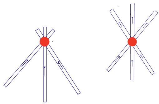
Figure 1. Illustration at time $t<0$ and time $t=0$ of the $x$-support of $f_{\text{b}}(x,v,t)$ in blue and $f_{\text{r}}(x,v,t)$ in red. The function $f_{\text{b}}$ consists of $\sim(MN_{2})^{2}$ tubes; here three typical tubes are depicted. Each tube moves in the direction of its long dimension. The ill-posedness part of Theorem 1.3 exploits solutions of the form is $f=f_{\text{b}}+f_{\text{r}}+f_{\text{c}}$, where $f_{\text{c}}$ is a small correction. As time evolves forward, the loss collision term between $f_{\text{b}}$ and $f_{\text{r}}$ drives the amplitude of $f_{\text{r}}$ downward exponentially fast.

Per Theorem 1.3, these impolsion / cavity like solutions are obstacles to the well-posedness for $s<1$ while they do not pose any problems for $s>1$. We wonder if this phenomenon is related to the fact that, though more difficult to solve, the Boltzmann equation is preferred over its various scaling limits, like the compressible Euler equation for example, in some aspects of engineering like the aerodynamics at hypersonic speed for example. These “bad” solutions arise from the sharpness examples of the bilinear $X_{s,b}$ estimate stated below as Theorem 1.4.

Theorem 1.4 (loss term bilinear estimate and sharpness example).

Let $\theta(t)$ be a smooth function such that $\theta(t)=1$ on $-1\leq t\leq 1$ and $\mathop{\mathrm{s}upp}\theta\subset[-2,2]$. For $\hat{f}$ supported in the dyadic regions $|\eta_{1}|\sim M_{1}\geq 1$, $|v_{1}|\sim N\geq 1$, and $\hat{g}$ supported in the dyadic regions $|\eta_{2}|\sim M_{2}\geq 1$, $|v_{2}|\sim N_{2}\geq 1$,

(1.12) $$\|\theta(t)\tilde{Q}^{-}(\tilde{f},\tilde{g})\|_{X_{0,-\frac{1}{2}+}}\lesssim\min(M_{1},M_{2})^{1+}N_{2}^{1+}B_{M_{1},M_{2}}^{1-}B_{N,N_{2}}^{1-}\|\tilde{f}\|_{X_{0,\frac{1}{2}+}}\|\tilde{g}\|_{X_{0,\frac{1}{2}+}}$$

where $B_{M_{1},M_{2}}$ and $B_{N,N_{2}}$ are the one-sided bilinear gain factors

$$B_{M_{1},M_{2}}=\begin{cases}\left(\frac{M_{1}}{M_{2}}\right)^{1/2}&\text{if }M_{1}\leq M_{2}\\ 1&\text{if }M_{1}\geq M_{2}\end{cases}\,,\qquad B_{N,N_{2}}=\begin{cases}\left(\frac{N_{2}}{N}\right)^{1/2}&\text{if }N_{2}\leq N\\ 1&\text{if }N_{2}\geq N\end{cases}$$

It follows that for any $s>1$, for any $f$ and $g$ (without frequency support restrictions),

(1.13) $$\|\theta(t)\tilde{Q}^{-}(\tilde{f},\tilde{g})\|_{X_{s,-\frac{1}{2}+}}\lesssim\|\tilde{f}\|_{X_{s,\frac{1}{2}+}}\|\tilde{g}\|_{X_{s,\frac{1}{2}+}}$$

There exist functions $f$ and $g$ with $\hat{f}$ supported in the dyadic regions $|\eta_{1}|\sim M_{1}$, $|v_{1}|\sim N$, and $\hat{g}$ supported in the dyadic regions $|\eta_{2}|\sim M_{2}$, $|v_{2}|\sim N_{2}$, such that

$$\max(N,1)\ll N_{2}\,\quad M_{1}\geq 1\,,\quad M_{2}\geq 1$$

and

(1.14) $$\|\theta(t)\tilde{Q}^{-}(\tilde{f},\tilde{g})\|_{X_{0,-b^{\prime}}}\gtrsim\min(M_{1},M_{2})N_{2}B_{M_{1}M_{2}}\|\tilde{f}\|_{X_{0,b_{1}}}\|\tilde{g}\|_{X_{0,b_{2}}}$$

for all $b^{\prime},b_{1},b_{2}\in\mathbb{R}$.

We emphasize that the bilinear gain factors, typically present in these types of estimates, are both only one-sided in this case. This comes from the fact that the loss operator $Q^{-}$ is highly nonsymmetric in $f$ and $g$, and not of convolution type in the variable $v$. Estimate (1.13), which is (1.12) without the bilinear gain factors, can be proved rather quickly using the Strichartz estimates, but to see the “bad” solutions, one has to study (1.12) and how it becomes saturated.

In contrast to the loss term, the gain term has bilinear estimates which almost match the critical scaling $s=\frac{1}{2}$.

Theorem 1.5.

Let $\theta(t)$ be a smooth function such that $\theta(t)=1$ on $-1\leq t\leq 1$ and $\mathop{\mathrm{s}upp}\theta\subset[-2,2]$. For all $s>\frac{1}{2}$, for any $f$ and $g$ (without frequency support restrictions),

(1.15) $$\|\theta(t)\tilde{Q}^{+}(\tilde{f},\tilde{g})\|_{X_{s,-\frac{1}{2}+}}\lesssim\|\tilde{f}\|_{X_{s,\frac{1}{2}+}}\|\tilde{g}\|_{X_{s,\frac{1}{2}+}}$$

The $s=\frac{1}{2}$ case of (1.15) might also be correct, but it cannot change the ill-posedness facts even if it is, due to the loss term. That is, in low regularity settings, the gain term is like an error, compared to the loss term. Or in other words, the long expected cancelation between the gain and loss terms does not happen. Such a disparity between the gain term and the loss term ultimately creates Theorem 1.3.

1.1. Organization of the Paper

The novelty of this paper lies in Theorem 1.3 which establishes the well/ill-posedness seperation and proves the ill-posedness. Because the ill-posedness happens at scaling subcritical regime, ordinary scaling or perturbative methods for scaling critical or supercritical regimes fail here. We thus need new ideas addressing the full nonlinear equation. The 1st step would be getting sharp estimates.

In §2, we prove (1.13) in Theorem 1.4 by appealing to the Strichartz estimates (reviewed in Appendix A) and prove the sharpness of (1.12) from which the illposedness originates. The proof of (1.12) is available upon request as it needs a lengthy and direct analysis of frequency interactions involving a conic decomposition of $v$-space and a dual wedge decomposition of $\eta$-space. In §3, we prove the gain term estimates in Theorem 1.5 by appealing to a Hölder type estimate in [3] together with a Littlewood-Paley decomposition. For completeness, we apply in the short section §4, the loss term estimate in Theorem 1.4 and the gain term estimate in Theorem 1.5 to prove the well-posedness part of Theorem 1.3.

We prove the illposedness part of Theorem 1.3 in §5. We work on the more usual $(x,v)$ side of (1.2) throughout §5 but it is still very much based on $X_{s,b}$ theory. As the proof involves many delicate computations, we 1st provide a heuristic using the sharpness example of (1.12), suitably scaled, in §5.1, then we present the approximate solutions / ansatz $f_{a}$ we are going to use in §5.2. We use a specialized perturbative argument, built around $f_{a}$, to prove that there is an exact solution to (1.2) which is mostly $f_{a}$. We put down the tools in §5.3 to §5.5 to conclude the perturbative argument in §5.6. During the estimate of the error terms, the proof involves many geometric techniques, like the ones in $X_{s,b}$ theory (See, for example, [40, 53]), on the fine nonlinear interactions. A good example would be §5.4.4. Such a connection between the analysis of (1.2) and the dispersive equations might be highly nontrivial and deserves further investigations. We then conclude the ill-posedness and the norm deflation in Corollaries 5.5 and 5.6.

After the proof of the main theorem in §5, we include in Appendix A a discusion of the scaling properties of (1.2) and review the Strichartz estimates.

Acknowledgement The authors would like to thank Yan Guo for multiple discussions and encouragements about this work.

2. Loss term bilinear estimate and its sharpness

In this section, we prove (1.13), the simpler version of the full optimal bilinear estimate (1.12), and establish the sharpness of (1.12). We leave out the proof of (1.12) in this paper as it is highly technical and not directly used while its sharpness has made the illposedness possible. The logical order, as it has happened, was, proving (1.12) $\rightarrow$ finding examples to saturate (1.12) $\rightarrow$ ill-posedness, and one would not have come up with the ill-posedness without the 1st step.

2.1. Proof of (1.13)

It suffices to prove

$$\left\|\tilde{Q}^{-}(\tilde{f},\tilde{g})\right\|_{L_{t}^{2}H_{x\xi}^{s}}\lesssim\|\tilde{f}\|_{X_{s,\frac{1}{2}+}}\|\tilde{g}\|_{X_{s,\frac{1}{2}+}}$$

for $s>1$. Recall (1.9),

$$\left\|\tilde{Q}^{-}(\tilde{f},\tilde{g})\right\|_{L_{t}^{2}H_{x\xi}^{s}}=\left\|\left\langle\nabla_{x}\right\rangle^{s}\left(\left\langle\nabla_{\xi}\right\rangle^{s}\tilde{f}(t,x,\xi)\tilde{g}(t,x,0)\right)\right\|_{L_{t}^{2}L_{x\xi}^{2}}$$

Splitting into the two cases in which $\tilde{f}$ or $\tilde{g}$ has the dominating frequency, we have

$$\left\|\tilde{Q}^{-}(\tilde{f},\tilde{g})\right\|_{L_{t}^{2}H_{x\xi}^{s}} \lesssim \left\|\left(\left\langle\nabla_{x}\right\rangle^{s}\left\langle\nabla_{\xi}\right\rangle^{s}\tilde{f}(t,x,\xi)\right)\tilde{g}(t,x,0)\right\|_{L_{t}^{2}L_{x\xi}^{2}}$$

$$+\left\|\left(\left\langle\nabla_{\xi}\right\rangle^{s}\tilde{f}(t,x,\xi)\right)\left\langle\nabla_{x}\right\rangle^{s}\tilde{g}(t,x,0)\right\|_{L_{t}^{2}L_{x\xi}^{2}}$$

Apply Hölder,

$$\left\|\tilde{Q}^{-}(\tilde{f},\tilde{g})\right\|_{L_{t}^{2}H_{x\xi}^{s}} \lesssim \left\|\left\langle\nabla_{x}\right\rangle^{s}\left\langle\nabla_{\xi}\right\rangle^{s}\tilde{f}(t,x,\xi)\right\|_{L_{t}^{\infty}L_{x\xi}^{2}}\left\|\tilde{g}(t,x,\xi)\right\|_{L_{t}^{2}L_{x\xi}^{\infty}}$$

$$+\left\|\left\langle\nabla_{\xi}\right\rangle^{s}\tilde{f}(t,x,\xi)\right\|_{L_{t}^{\infty}L_{x}^{6}L_{\xi}^{2}}\left\|\left\langle\nabla_{x}\right\rangle^{s}\tilde{g}(t,x,\xi)\right\|_{L_{t}^{2}L_{x}^{3}L_{\xi}^{\infty}}$$

Use $s>1$ and apply Sobolev,

$$\left\|\tilde{Q}^{-}(\tilde{f},\tilde{g})\right\|_{L_{t}^{2}H_{x\xi}^{s}}\lesssim\left\|\left\langle\nabla_{x}\right\rangle^{s}\left\langle\nabla_{\xi}\right\rangle^{s}\tilde{f}(t,x,\xi)\right\|_{L_{t}^{\infty}L_{x\xi}^{2}}\left\|\left\langle\nabla_{x}\right\rangle^{s}\left\langle\nabla_{\xi}\right\rangle^{s}\tilde{g}(t,x,\xi)\right\|_{L_{t}^{2}L_{x\xi}^{3}}$$

Apply Strichartz (1.5), we have

$$\left\|\tilde{Q}^{-}(\tilde{f},\tilde{g})\right\|_{L_{t}^{2}H_{x\xi}^{s}}\lesssim\|\tilde{f}\|_{X_{s,\frac{1}{2}+}}\|\tilde{g}\|_{X_{s,\frac{1}{2}+}}$$

as claimed.

2.2. Proof of Sharpness

At this point, we turn to the sharpness example. The example is inspired by the steps of the proof of (1.12) in Theorem 1.4. (Available upon request.) We will consider $|\eta_{2}|\sim M_{2}$ and $|v_{2}|\sim N_{2}$, with $M_{2}\gg 1$ and $N_{2}\gg 1$ dyadic. On the unit sphere, lay down a grid of $J\sim M_{2}^{2}N_{2}^{2}$ points $\{e_{j}\}_{j=1}^{J}$, where the points $e_{j}$ are roughly equally spaced and each have their own neighborhood of unit-sphere surface area $\sim M_{2}^{-1}N_{2}^{-1}$. Let $P_{e_{j}}$ denote the orthogonal projection onto the 1D subspace spanned by $e_{j}$. Let $P_{e_{j}}^{\perp}$ denote the orthogonal projection onto the 2D subspace $\mathop{\mathrm{s}pan}\{e_{j}\}^{\perp}$.

For each $e_{j}$, let $B_{j}$ denote, in $v_{2}$ space, the conic neighborhood of $e_{j}$ obtained by taking all radial rays passing though the patch of surface area $M_{2}^{-1}N_{2}^{-1}$ on the unit sphere around the vector $e_{j}$. We can describe this as the cone with vertex $e_{j}$ and angular aperture $M_{2}^{-1}N_{2}^{-1}$. When this cone, in $v_{2}$-space, intersects the dyadic annulus at radius $\sim N_{2}$, it creates a shape that is approximately a cube with long side $N_{2}$ and two shorter dimensions each of length $M_{2}^{-1}$. For convenience we think of it as a cube with shape $M_{2}^{-1}\times M_{2}^{-1}\times N_{2}$, with the line through $e_{j}$ passing through the axis and parallel to the long side.

For each $e_{j}$, in $\eta_{2}$ space, let $A_{j}$ consist of all vectors $\eta_{2}$ that are “nearly perpendicular” to $e_{j}$, in the sense that the cosine of the angle between $e_{j}$ and $\eta_{2}/|\eta_{2}|$ is

$$\cos(e_{j},\frac{\eta_{2}}{|\eta_{2}|})\lesssim\frac{1}{M_{2}N_{2}}$$

Since $\sin(90^{\circ}-\theta)=\cos(\theta)$, this means that the angle between $e_{j}$ and any vector $\eta_{2}\in A_{j}$ is within $M_{2}^{-1}N_{2}^{-1}$ of $90$ degrees. This property then clearly extends to replacing $e_{j}$ with any vector in $B_{j}$. We can then visualize $B_{j}$, projected onto the unit sphere, as being obtained by taking the plane perpendicular to $e_{j}$, calling that the “equator”, and then taking the band that is width $M_{2}^{-1}N_{2}^{-1}$ around that equator. When $A_{j}$ is intersected with the dyadic annulus at radius $\sim M_{2}$, this set looks like a thickened plane of width $N_{2}^{-1}$, so it has approximate dimensions $M_{2}\times M_{2}\times N_{2}^{-1}$, where the $M_{2}\times M_{2}$ planar part is perpendicular to $e_{j}$. ($A_{j}$ looks like the so-called bevelled washer.)

The example proving (1.14) in Theorem 1.4 is produced as follows. Let $\hat{\chi}(\eta)$ (or $\hat{\chi}(v)$) be a smooth nonnegative compactly supported function such that $\hat{\chi}(0)=1$. We present the functions $\tilde{\phi}$ and $\tilde{\psi}$ as normalized in $L^{2}_{x}L^{2}_{\xi}$.

$$\hat{\phi}(\eta_{1},v)=\frac{1}{M_{1}^{3/2}N^{3/2}}\hat{\chi}(\frac{\eta_{1}}{M_{1}})\hat{\chi}(\frac{v}{N})$$

$$\hat{\psi}(\eta_{2},v_{2})=\frac{1}{M_{2}N_{2}}\sum_{j=1}^{J}\hat{\chi}\left(\frac{P_{e_{j}}^{\perp}\eta_{2}}{M_{2}}\right)\hat{\chi}(N_{2}P_{e_{j}}\eta_{2})\hat{\chi}(M_{2}P_{e_{j}}^{\perp}v_{2})\hat{\chi}(\frac{P_{e_{j}}v_{2}}{N_{2}})$$

where $J\sim M_{2}^{2}N_{2}^{2}$. Since we are proving a lower bound, we can select any normalized dual function $\tilde{\zeta}\in L_{x}^{2}L_{\xi}^{2}$. We select

$$\hat{\zeta}(\eta,v)=\frac{1}{\max(M_{1},M_{2})^{3/2}N^{3/2}}\hat{\chi}(\frac{\eta}{\max(M_{1},M_{2})})\hat{\chi}(\frac{v}{N})$$

Then let

(2.1) $$I=\int_{\eta}\int_{\eta_{2}}\int_{v}\int_{v_{2}}\hat{\theta}(-\eta_{2}\cdot(v-v_{2}))\,\hat{\phi}(\eta-\eta_{2},v)\,\hat{\psi}(\eta_{2},v_{2})\,\overline{\hat{\zeta}(\eta,v)}\,dv_{2}\,dv\,d\eta_{2}\,d\eta$$

and we aim to prove

$$I\gtrsim\min(M_{1},M_{2})N_{2}B_{M_{1}M_{2}}\|\hat{\phi}\|_{L^{2}_{\eta_{1}v}}\|\hat{\psi}\|_{L^{2}_{\eta_{2}v_{2}}}\|\hat{\zeta}\|_{L^{2}_{\eta v}}$$

We are restricting to $M_{1}\geq 1$, $M_{2}\geq 1$ and $N\leq M^{-1}\ll 1\ll N_{2}$ but otherwise do not assume any relationship between $M_{1}$ and $M_{2}$. The argument can be extended to weaken the restriction on $N$ to only $N\ll N_{2}$. (Available upon request.)

To carry out the computation, we need to introduce $C_{k}$, subsets of $\eta_{2}$ space, which are cones with angular aperture $M_{2}^{-1}N_{2}^{-1}$ with vertex vector $e_{k}$. (That is, $C_{k}$ for $k=1,\ldots,M_{2}^{2}N_{2}^{2}$ is the same type of decomposition of $\eta_{2}$ space as the decomposition $B_{j}$, $j=1,\ldots,M_{2}^{2}N_{2}^{2}$ of $v_{2}$-space, except that in the case of $\{C_{k}\}$, the cones intersect the $M_{2}$ dyad, and in the case $\{B_{j}\}$, the cones intersect the $N_{2}$ dyad.). The cone $C_{k}$ intersects the $M_{2}$ dyad in $\eta_{2}$ space in a tube of geometry $N_{2}^{-1}\times N_{2}^{-1}\times M_{2}$, whereas the cone $B_{j}$ intersects the $N_{2}$ dyad in $v_{2}$ space in a tube of geometry $M_{2}^{-1}\times M_{2}^{-1}\times N_{2}$.

For each $j$ and corresponding direction $e_{j}$, there are $\sim M_{2}N_{2}$ directions $e_{k}$ that are perpendicular to $e_{j}$ – let us call this set $K(j)$. Then we have that for each $j$, the thickened planes/beveled washers $A_{j}$ are:

$$A_{j}=\bigcup_{k\in K(j)}C_{k}$$

We can now look at this in the other direction as well – fix $k$ and corresponding direction $e_{k}$. There are $\sim M_{2}N_{2}$ directions $e_{j}$ that are perpendicular to $e_{k}$ – call this set of indices $J(k)$. The union of these becomes a thickened plane/beveled washer in $v_{2}$ space.

Now we carry out the integral in (2.1) by first noting that since $N\ll N_{2}$, $v_{2}-v$ can effectively be replaced by $v_{2}$ in $\hat{\theta}(\eta_{2}\cdot(v_{2}-v))$. This allows us to simply carry out the $v$ and $v_{2}$ integration after enforcing the orthogonality of $v_{2}$ and $\eta_{2}$ through restriction to appropriate sets $B_{j}$ and $C_{k}$, respectively.

(2.2) $$I=\int_{\eta}\int_{\eta_{2}}\left(\int_{v}\hat{\phi}(\eta-\eta_{2},v)\hat{\zeta}(\eta,v)\,dv\sum_{k}\boldsymbol{1}_{C_{k}}(\eta_{2})\sum_{j\in J(k)}\int_{v_{2}}\boldsymbol{1}_{B_{j}}(v_{2})\hat{\psi}(\eta_{2},v_{2})\,dv_{2}\right)\,d\eta_{2}\,d\eta$$

The components inside (2.2) are

$$\int_{v}\hat{\phi}(\eta-\eta_{2},v)\hat{\zeta}(\eta,v)\,dv=\frac{1}{M_{1}^{3/2}\max(M_{1},M_{2})^{3/2}}\hat{\chi}(\frac{\eta-\eta_{1}}{M_{1}})\hat{\chi}(\frac{\eta}{\max(M_{1},M_{2})})$$

and

(2.3) $$\sum_{k}\sum_{j\in J(k)}\boldsymbol{1}_{C_{k}}(\eta_{2})\int_{v_{2}}\boldsymbol{1}_{B_{j}}(v_{2})\hat{\psi}(\eta_{2},v_{2})\,dv_{2}=\frac{1}{M_{2}^{3}}\sum_{k}\sum_{j\in J(k)}\boldsymbol{1}_{C_{k}}(\eta_{2})\hat{\chi}\left(\frac{P_{e_{j}}^{\perp}\eta_{2}}{M_{2}}\right)\hat{\chi}(N_{2}P_{e_{j}}\eta_{2})$$

For (2.3), consider that $\hat{\chi}\left(\frac{P_{e_{j}}^{\perp}\eta_{2}}{M_{2}}\right)\hat{\chi}(N_{2}P_{e_{j}}\eta_{2})$ is basically $\boldsymbol{1}_{A_{j}}(\eta_{2})$, but since $e_{k}$ and $e_{j}$ are perpendicular, it follows that $C_{k}\subset A_{j}$ and $\boldsymbol{1}_{C_{k}}(\eta_{2})\boldsymbol{1}_{A_{j}}(\eta_{2})=\boldsymbol{1}_{C_{k}}(\eta_{2})$. Thus we continue the evaluation as

$$\sum_{k}\sum_{j\in J(k)}\boldsymbol{1}_{C_{k}}(\eta_{2})\int_{v_{2}}\boldsymbol{1}_{B_{j}}(v_{2})\hat{\psi}(\eta_{2},v_{2})\,dv_{2}=\frac{1}{M_{2}^{3}}\sum_{k}\sum_{j\in J(k)}\boldsymbol{1}_{C_{k}}(\eta_{2})$$

$$=\frac{1}{M_{2}^{3}}\sum_{k}\mathop{\mathrm{c}ard}J(k)\boldsymbol{1}_{C_{k}}(\eta_{2})=\frac{N_{2}}{M_{2}^{2}}\sum_{k}\boldsymbol{1}_{C_{k}}(\eta_{2})=\frac{N_{2}}{M_{2}^{2}}\hat{\chi}(\frac{\eta_{2}}{M_{2}})$$

where $\mathop{\mathrm{c}ard}(A)$ of a set $A$ means the cardinality of set $A$. That is, since $\{C_{k}\}$ just partitions the whole $M_{2}$ dyad, we end up with simply the projection onto the whole dyad. Plugging these results back into (2.2),

$$I=\int_{\eta}\int_{\eta_{2}}\frac{1}{M_{1}^{3/2}\max(M_{1},M_{2})^{3/2}}\hat{\chi}(\frac{\eta-\eta_{1}}{M_{1}})\hat{\chi}(\frac{\eta}{\max(M_{1},M_{2})})\frac{N_{2}}{M_{2}^{2}}\hat{\chi}(\frac{\eta_{2}}{M_{2}})\,d\eta_{2}\,d\eta$$

Now we revert back to the spatial side via Plancherel:

$$I=M_{1}^{3/2}\max(M_{1},M_{2})^{3/2}M_{2}N_{2}\int_{x}\chi(M_{1}x)\chi(\max(M_{1},M_{2})x)\chi(M_{2}x)\,dx$$

The function $\chi(\max(M_{1},M_{2})x)$ is redundant, and the $x$-integral evaluates to $\max(M_{1},M_{2})^{-3}$. Thus

$$I=\frac{M_{1}^{3/2}M_{2}N_{2}}{\max(M_{1},M_{2})^{3/2}}=\min(M_{1},M_{2})N_{2}B_{M_{1}M_{2}}$$

which is precisely the lower bound in the statement of Theorem 1.4.

3. Gain term bilinear estimate

We prove Theorem 1.5 in this section. We will need the following lemma.

Lemma 3.1 (Hölder Inequality for $\tilde{Q}^{+}$).

Let $\frac{1}{p}+\frac{1}{q}=\frac{1}{r}$ where $p,q>\frac{3}{2}$ and let $b(\frac{\xi}{\left|\xi\right|},\omega)\in C\left(\mathbb{S}^{2}\times\mathbb{S}^{2}\right)$, we then have the estimate that

$$\left\|\int_{\mathbb{S}^{2}}\tilde{f}(\xi^{+})\tilde{g}(\xi^{-})b(\frac{\xi}{\left|\xi\right|},\omega)d\omega\right\|_{L_{\xi}^{r}}\lesssim\left\|\tilde{f}\right\|_{L_{\xi}^{p}}\left\|\tilde{g}\right\|_{L_{\xi}^{q}}$$

Proof.

This is actually a small modification of a special case of [3, Theorem 1]. Their proof actually works for all uniformly bounded $b$ with little modification. We omit the details here.    

Denote the Littlewood-Paley projector of $x/\xi$ at frequency $N/M$ by $P_{N}^{x}/P_{M}^{\xi}$. We will use Lemma 3.1 in the following format.

Lemma 3.2.

Let $\frac{1}{p}+\frac{1}{q}=\frac{1}{r}$ where $p,q>\frac{3}{2}$, we then have

$$\left\|P_{N}^{x}P_{M}^{\xi}\tilde{Q}^{+}\left(P_{N_{1}}^{x}P_{M_{1}}^{\xi}\tilde{f},P_{N_{2}}^{x}P_{M_{2}}^{\xi}\tilde{g}\right)\right\|_{L_{\xi}^{r}} \lesssim \min(1,\frac{\max(N_{1},N_{2})}{N})\min(1,\frac{\max(M_{1},M_{2})}{M})$$

$$\times\left\|P_{N_{1}}^{x}P_{M_{1}}^{\xi}\tilde{f}\right\|_{L_{\xi}^{p}}\left\|P_{N_{2}}^{x}P_{M_{2}}^{\xi}\tilde{g}\right\|_{L_{\xi}^{q}}$$

Proof.

The estimate can be obtained by interpolating the four inequalities:

$$\left\|P_{N}^{x}P_{M}^{\xi}\tilde{Q}^{+}\left(P_{N_{1}}^{x}P_{M_{1}}^{\xi}\tilde{f},P_{N_{2}}^{x}P_{M_{2}}^{\xi}\tilde{g}\right)\right\|_{L_{\xi}^{r}}\lesssim\left\|P_{N_{1}}^{x}P_{M_{1}}^{\xi}\tilde{f}\right\|_{L_{\xi}^{p}}\left\|P_{N_{2}}^{x}P_{M_{2}}^{\xi}\tilde{g}\right\|_{L_{\xi}^{q}}$$

$$\left\|P_{N}^{x}P_{M}^{\xi}\tilde{Q}^{+}\left(P_{N_{1}}^{x}P_{M_{1}}^{\xi}\tilde{f},P_{N_{2}}^{x}P_{M_{2}}^{\xi}\tilde{g}\right)\right\|_{L_{\xi}^{r}}\lesssim\frac{\max(M_{1},M_{2})}{M}\left\|P_{N_{1}}^{x}P_{M_{1}}^{\xi}\tilde{f}\right\|_{L_{\xi}^{p}}\left\|P_{N_{2}}^{x}P_{M_{2}}^{\xi}\tilde{g}\right\|_{L_{\xi}^{q}}$$

$$\left\|P_{N}^{x}P_{M}^{\xi}\tilde{Q}^{+}\left(P_{N_{1}}^{x}P_{M_{1}}^{\xi}\tilde{f},P_{N_{2}}^{x}P_{M_{2}}^{\xi}\tilde{g}\right)\right\|_{L_{\xi}^{r}}\lesssim\frac{\max(N_{1},N_{2})}{N}\left\|P_{N_{1}}^{x}P_{M_{1}}^{\xi}\tilde{f}\right\|_{L_{\xi}^{p}}\left\|P_{N_{2}}^{x}P_{M_{2}}^{\xi}\tilde{g}\right\|_{L_{\xi}^{q}}$$

$$\left\|P_{N}^{x}P_{M}^{\xi}\tilde{Q}^{+}\left(P_{N_{1}}^{x}P_{M_{1}}^{\xi}\tilde{f},P_{N_{2}}^{x}P_{M_{2}}^{\xi}\tilde{g}\right)\right\|_{L_{\xi}^{r}} \lesssim \frac{\max(N_{1},N_{2})}{N}\frac{\max(M_{1},M_{2})}{M}$$

$$\times\left\|P_{N_{1}}^{x}P_{M_{1}}^{\xi}\tilde{f}\right\|_{L_{\xi}^{p}}\left\|P_{N_{2}}^{x}P_{M_{2}}^{\xi}\tilde{g}\right\|_{L_{\xi}^{q}}$$

The main concern is definitely the $\xi$-part as $\tilde{Q}^{+}$ commutes with $P_{N}^{x}$ and $\nabla_{x},$ it suffices to prove

(3.1) $$\left\|P_{M}^{\xi}\tilde{Q}^{+}\left(P_{M_{1}}^{\xi}\tilde{f},P_{M_{2}}^{\xi}\tilde{g}\right)\right\|_{L_{\xi}^{r}}\lesssim\left\|P_{M_{1}}^{\xi}\tilde{f}\right\|_{L_{\xi}^{p}}\left\|P_{M_{2}}^{\xi}\tilde{g}\right\|_{L_{\xi}^{q}},$$

and

(3.2) $$\left\|P_{M}^{\xi}\tilde{Q}^{+}\left(P_{M_{1}}^{\xi}\tilde{f},P_{M_{2}}^{\xi}\tilde{g}\right)\right\|_{L_{\xi}^{r}}\lesssim\frac{\max(M_{1},M_{2})}{M}\left\|P_{M_{1}}^{\xi}\tilde{f}\right\|_{L_{\xi}^{p}}\left\|P_{M_{2}}^{\xi}\tilde{g}\right\|_{L_{\xi}^{q}}.$$

While (3.1) is directly from Lemma 3.1, we prove only (3.2). Notice that

$$\partial_{\xi_{j}}\left(\tilde{f}(\xi^{+})\tilde{g}(\xi^{-})\right)=\left(\partial_{\xi_{j}}\tilde{f}\right)(\xi^{+})\tilde{g}(\xi^{-})\partial_{\xi_{j}}\xi^{+}+\tilde{f}(\xi^{+})\left(\partial_{\xi_{j}}\tilde{g}\right)(\xi^{-})\partial_{\xi_{j}}\xi^{-}$$

and $\left|\partial_{\xi_{j}}\xi^{\pm}\right|\leqslant 1$, we can thus apply Lemma 3.1 with $b=\partial_{\xi_{j}}\xi^{\pm}$. That is,

$$\left\|P_{M}^{\xi}\tilde{Q}^{+}\left(P_{M_{1}}^{\xi}\tilde{f},P_{M_{2}}^{\xi}\tilde{g}\right)\right\|_{L_{\xi}^{r}}$$

$$= M^{-1}\left\|P_{M}^{\xi}\nabla_{\xi}\tilde{Q}^{+}\left(P_{M_{1}}^{\xi}\tilde{f},P_{M_{2}}^{\xi}\tilde{g}\right)\right\|_{L_{\xi}^{r}}$$

$$\lesssim M^{-1}\left(\left\|P_{M_{1}}^{\xi}\nabla_{\xi}\tilde{f}\right\|_{L_{\xi}^{p}}\left\|P_{M_{2}}^{\xi}\tilde{g}\right\|_{L_{\xi}^{q}}+\left\|P_{M_{1}}^{\xi}\tilde{f}\right\|_{L_{\xi}^{p}}\left\|P_{M_{2}}^{\xi}\nabla_{\xi}\tilde{g}\right\|_{L_{\xi}^{q}}\right)$$

which, by Bernstein, is

$$\left\|P_{M}^{\xi}\tilde{Q}^{+}\left(P_{M_{1}}^{\xi}\tilde{f},P_{M_{2}}^{\xi}\tilde{g}\right)\right\|_{L_{\xi}^{r}}\lesssim\frac{\max(M_{1},M_{2})}{M}\left\|P_{M_{1}}^{\xi}\tilde{f}\right\|_{L_{\xi}^{p}}\left\|P_{M_{2}}^{\xi}\tilde{g}\right\|_{L_{\xi}^{q}}$$

as claimed in (3.2).    

3.1. Proof of Theorem 1.5

It suffice to prove

$$\|\left\langle\nabla_{x}\right\rangle^{s}\left\langle\nabla_{\xi}\right\rangle^{s}\tilde{Q}^{+}(\tilde{f},\tilde{g})\|_{L_{t}^{1}L_{x\xi}^{2}}\lesssim\|\tilde{f}\|_{X_{s,\frac{1}{2}+}}\|\tilde{g}\|_{X_{s,\frac{1}{2}+}}\text{.}$$

We start by decomposing $\tilde{Q}^{+}(f,g)$ into Littlewood-Paley pieces

$$\|\left\langle\nabla_{x}\right\rangle^{s}\left\langle\nabla_{\xi}\right\rangle^{s}\tilde{Q}^{+}(\tilde{f},\tilde{g})\|_{L_{t}^{1}L_{x\xi}^{2}}$$

$$\leqslant \sum_{\begin{subarray}{c}M,M_{1}M_{2}\\ N,N_{1},N_{2}\end{subarray}}M^{s}N^{s}\|P_{N}^{x}P_{M}^{\xi}\tilde{Q}^{+}\left(P_{N_{1}}^{x}P_{M_{1}}^{\xi}\tilde{f},P_{N_{2}}^{x}P_{M_{2}}^{\xi}\tilde{g}\right)\|_{L_{t}^{1}L_{x\xi}^{2}}$$

$$= A+B+C+D$$

where we have seperated the sum into 4 cases in which case A is $M_{1}\geqslant M_{2}$, $N_{1}\geqslant N_{2}$, case $B$ is $M_{1}\leqslant M_{2}$, $N_{1}\geqslant N_{2}$, case $C$ is $M_{1}\leqslant M_{2}$, $N_{1}\leqslant N_{2}$, and case $D$ is $M_{1}\geqslant M_{2}$, $N_{1}\leqslant N_{2}$. We handle only cases A and B as the other two cases follow similarly.

3.1.1. Case A: $M_{1}\geqslant M_{2}$, $N_{1}\geqslant N_{2}$

$$A\lesssim\sum_{\begin{subarray}{c}{}_{\begin{subarray}{c}M,M_{1}M_{2}\\ N,N_{1},N_{2}\end{subarray}}\\ M_{1}\geqslant M_{2},N_{1}\geqslant N_{2}\end{subarray}}\frac{M^{s}N^{s}}{M_{1}^{s}N_{1}^{s}}\|P_{N}^{x}P_{M}^{\xi}\tilde{Q}^{+}\left(P_{N_{1}}^{x}P_{M_{1}}^{\xi}\left\langle\nabla_{x}\right\rangle^{s}\left\langle\nabla_{\xi}\right\rangle^{s}\tilde{f},P_{N_{2}}^{x}P_{M_{2}}^{\xi}\tilde{g}\right)\|_{L_{t}^{1}L_{x\xi}^{2}}$$

Use Lemma 3.2 and Hölder,

$$A \lesssim \sum_{\begin{subarray}{c}{}_{\begin{subarray}{c}M,M_{1}M_{2}\\ N,N_{1},N_{2}\end{subarray}}\\ M_{1}\geqslant M_{2},N_{1}\geqslant N_{2}\end{subarray}}\frac{M^{s}N^{s}}{M_{1}^{s}N_{1}^{s}}\min(1,\frac{N_{1}}{N})\min(1,\frac{M_{1}}{M})$$

$$\times\|P_{N_{1}}^{x}P_{M_{1}}^{\xi}\left\langle\nabla_{x}\right\rangle^{s}\left\langle\nabla_{\xi}\right\rangle^{s}\tilde{f}\|_{L_{t}^{2}L_{x\xi}^{3}}\|P_{N_{2}}^{x}P_{M_{2}}^{\xi}\tilde{g}\|_{L_{t}^{2}L_{x\xi}^{6}}.$$

By Sobolev and Bernstein,

$$A \lesssim \sum_{\begin{subarray}{c}{}_{\begin{subarray}{c}M,M_{1}M_{2}\\ N,N_{1},N_{2}\end{subarray}}\\ M_{1}\geqslant M_{2},N_{1}\geqslant N_{2}\end{subarray}}\frac{M^{s}N^{s}}{M_{1}^{s}N_{1}^{s}}\min(1,\frac{N_{1}}{N})\min(1,\frac{M_{1}}{M})$$

$$\times\|P_{N_{1}}^{x}P_{M_{1}}^{\xi}\left\langle\nabla_{x}\right\rangle^{s}\left\langle\nabla_{\xi}\right\rangle^{s}\tilde{f}\|_{L_{t}^{2}L_{x\xi}^{3}}\|P_{N_{2}}^{x}P_{M_{2}}^{\xi}\left\langle\nabla_{x}\right\rangle^{\frac{1}{2}}\left\langle\nabla_{\xi}\right\rangle^{\frac{1}{2}}\tilde{g}\|_{L_{t}^{2}L_{x\xi}^{3}}$$

$$\lesssim \sum_{\begin{subarray}{c}{}_{\begin{subarray}{c}M,M_{1}M_{2}\\ N,N_{1},N_{2}\end{subarray}}\\ M_{1}\geqslant M_{2},N_{1}\geqslant N_{2}\end{subarray}}\frac{M^{s}N^{s}}{M_{1}^{s}N_{1}^{s}}\min(1,\frac{N_{1}}{N})\min(1,\frac{M_{1}}{M})\frac{1}{N_{2}^{s-\frac{1}{2}}}\frac{1}{M_{2}^{s-\frac{1}{2}}}$$

$$\times\|P_{N_{1}}^{x}P_{M_{1}}^{\xi}\left\langle\nabla_{x}\right\rangle^{s}\left\langle\nabla_{\xi}\right\rangle^{s}\tilde{f}\|_{L_{t}^{2}L_{x\xi}^{3}}\|P_{N_{2}}^{x}P_{M_{2}}^{\xi}\left\langle\nabla_{x}\right\rangle^{s}\left\langle\nabla_{\xi}\right\rangle^{s}\tilde{g}\|_{L_{t}^{2}L_{x\xi}^{3}}$$

By Strichartz,

$$A \lesssim \sum_{\begin{subarray}{c}{}_{\begin{subarray}{c}M,M_{1}M_{2}\\ N,N_{1},N_{2}\end{subarray}}\\ M_{1}\geqslant M_{2},N_{1}\geqslant N_{2}\end{subarray}}\frac{M^{s}N^{s}}{M_{1}^{s}N_{2}^{s}}\min(1,\frac{N_{1}}{N})\min(1,\frac{M_{1}}{M})\frac{1}{N_{2}^{s-\frac{1}{2}}}\frac{1}{M_{2}^{s-\frac{1}{2}}}$$

$$\times\|P_{N_{1}}^{x}P_{M_{1}}^{\xi}\tilde{f}\|_{X_{s,\frac{1}{2}+}}\|P_{N_{2}}^{x}P_{M_{2}}^{\xi}\tilde{g}\|_{X_{s,\frac{1}{2}+}}\text{.}$$

Cauchy-Schwarz in $N_{2}$,$M_{2}$ to carry out the $N_{2}$,$M_{2}$ sum, we have

$$A\lesssim\|\tilde{g}\|_{X_{s,\frac{1}{2}+}}\sum_{{}_{\begin{subarray}{c}M,M_{1}\\ N,N_{1}\end{subarray}}}\frac{M^{s}N^{s}}{M_{1}^{s}N_{2}^{s}}\min(1,\frac{N_{1}}{N})\min(1,\frac{M_{1}}{M})\|P_{N_{1}}^{x}P_{M_{1}}^{\xi}f\|_{X_{s,\frac{1}{2}+}}$$

Seperate the sum into four cases $M_{1}\leqslant M,M_{1}\geqslant M,N_{1}\leqslant N$, and $N_{1}\geqslant N$, we are done by Schur’s test or Cauchy-Schwarz.

3.1.2. Case B: $M_{1}\leqslant M_{2}$, $N_{1}\geqslant N_{2}$

$$B\lesssim\sum_{\begin{subarray}{c}{}_{\begin{subarray}{c}M,M_{1}M_{2}\\ N,N_{1},N_{2}\end{subarray}}\\ M_{1}\leqslant M_{2},N_{1}\geqslant N_{2}\end{subarray}}\frac{M^{s}N^{s}}{M_{2}^{s}N_{1}^{s}}\|P_{N}^{x}P_{M}^{\xi}\tilde{Q}^{+}\left(P_{N_{1}}^{x}P_{M_{1}}^{\xi}\left\langle\nabla_{x}\right\rangle^{s}\tilde{f},P_{N_{2}}^{x}P_{M_{2}}^{\xi}\left\langle\nabla_{\xi}\right\rangle^{s}\tilde{g}\right)\|_{L_{t}^{1}L_{x\xi}^{2}}$$

Use Lemma 3.2 and Hölder,

$$B \lesssim \sum_{\begin{subarray}{c}{}_{\begin{subarray}{c}M,M_{1}M_{2}\\ N,N_{1},N_{2}\end{subarray}}\\ M_{1}\leqslant M_{2},N_{1}\geqslant N_{2}\end{subarray}}\frac{M^{s}N^{s}}{M_{2}^{s}N_{1}^{s}}\min(1,\frac{N_{1}}{N})\min(1,\frac{M_{2}}{M})$$

$$\times\|P_{N_{1}}^{x}P_{M_{1}}^{\xi}\left\langle\nabla_{x}\right\rangle^{s}\tilde{f}\|_{L_{t}^{2}L_{x}^{3}L_{\xi}^{6}}\|P_{N_{2}}^{x}P_{M_{2}}^{\xi}\left\langle\nabla_{\xi}\right\rangle^{s}\tilde{g}\|_{L_{t}^{2}L_{x}^{6}L_{\xi}^{3}}.$$

By Sobolev and Bernstein,

$$B \lesssim \sum_{\begin{subarray}{c}{}_{\begin{subarray}{c}M,M_{1}M_{2}\\ N,N_{1},N_{2}\end{subarray}}\\ M_{1}\leqslant M_{2},N_{1}\geqslant N_{2}\end{subarray}}\frac{M^{s}N^{s}}{M_{2}^{s}N_{1}^{s}}\min(1,\frac{N_{1}}{N})\min(1,\frac{M_{2}}{M})$$

$$\times\|P_{N_{1}}^{x}P_{M_{1}}^{\xi}\left\langle\nabla_{x}\right\rangle^{s}\left\langle\nabla_{\xi}\right\rangle^{\frac{1}{2}}\tilde{f}\|_{L_{t}^{2}L_{x\xi}^{3}}\|P_{N_{2}}^{x}P_{M_{2}}^{\xi}\left\langle\nabla_{x}\right\rangle^{\frac{1}{2}}\left\langle\nabla_{\xi}\right\rangle^{s}\tilde{g}\|_{L_{t}^{2}L_{x\xi}^{3}}$$

$$\lesssim \sum_{\begin{subarray}{c}{}_{\begin{subarray}{c}M,M_{1}M_{2}\\ N,N_{1},N_{2}\end{subarray}}\\ M_{1}\leqslant M_{2},N_{1}\geqslant N_{2}\end{subarray}}\frac{M^{s}N^{s}}{M_{2}^{s}N_{1}^{s}}\min(1,\frac{N_{1}}{N})\min(1,\frac{M_{2}}{M})\frac{1}{N_{2}^{s-\frac{1}{2}}}\frac{1}{M_{1}^{s-\frac{1}{2}}}$$

$$\times\|P_{N_{1}}^{x}P_{M_{1}}^{\xi}\left\langle\nabla_{x}\right\rangle^{s}\left\langle\nabla_{\xi}\right\rangle^{s}\tilde{f}\|_{L_{t}^{2}L_{x\xi}^{3}}\|P_{N_{2}}^{x}P_{M_{2}}^{\xi}\left\langle\nabla_{x}\right\rangle^{s}\left\langle\nabla_{\xi}\right\rangle^{s}\tilde{g}\|_{L_{t}^{2}L_{x\xi}^{3}}$$

One can then proceed in the exact same manner as in Case A. We omit the details.

4. Well-posedness

For completeness, we provide a quick (and not so complete) treatment of the well-posedness statement in Theorem 1.3 using (1.13) and (1.15). As mentioned before, this part is already proved in [11, 12]. We prove only the existence, uniqueness, and the Lipschitz continuity of the solution map here. The nonnegativity of $f$ follows from the persistance of regularity [12].

Write $R=2\left\|\tilde{f}_{0}\right\|_{H_{x\xi}^{s}}$ and let $\theta(t)$ be a smooth function such that $\theta(t)=1$ for all $\left|t\right|\leq 1$ and $\theta(t)=0$ for $\left|t\right|\geq 2$. Put $T=\delta\langle R\rangle^{-2}$, where $\delta>0$ is an absolute constant (selected depending upon constants appearing in the estimates such as (4.1) that we apply). The estimates (1.13) and (1.15) admit the following minor adjustments that account for restriction in time:

(4.1) $$\|\theta(\frac{t}{T})\tilde{Q}(\tilde{f},\tilde{g})\|_{X_{s,-\frac{1}{2}+}}\lesssim T^{1/2}\|\tilde{f}\|_{X_{s,\frac{1}{2}+}}\|\tilde{g}\|_{X_{s,\frac{1}{2}+}}\text{ for }s>1.$$

Denote $B=\left\{\tilde{f}:\|\tilde{f}\|_{X_{s,\frac{1}{2}+}}\leq R\right\}$ the ball of radius $R$ in $X_{s,\frac{1}{2}+}$ and introduce the nonlinear mapping $\Lambda:B\rightarrow\mathcal{S}^{\prime}$ given by

$$\Lambda(\tilde{f})=\theta(t)e^{it\nabla_{x}\cdot\nabla_{\xi}}\tilde{f}_{0}+D(\tilde{f},\tilde{f})\,,\qquad D(\tilde{f},\tilde{f})=\theta(t)\int_{0}^{t}e^{i(t-t^{\prime})\nabla_{x}\cdot\nabla_{\xi}}\theta(t^{\prime}/T)\tilde{Q}(\tilde{f}(t^{\prime}),\tilde{f}(t^{\prime}))\,dt^{\prime}.$$

A fixed point $\tilde{f}=\Lambda(\tilde{f})$ will satisfy (1.10)/(1.2) for $-T\leq t\leq T$. Using (4.1) one can show that

$$\Lambda:B\rightarrow B\,,\qquad\|\Lambda(\tilde{f})-\Lambda(\tilde{g})\|_{X_{s,\frac{1}{2}+}}\leq\tfrac{1}{2}\|\tilde{f}-\tilde{g}\|_{X_{s,\frac{1}{2}+}}$$

and thus $\Lambda$ is a contraction. From this it follows that there is a fixed point $\tilde{f}$ in $X_{s,\frac{1}{2}+}$, and this fixed point is unique in $X_{s,\frac{1}{2}+}$.

Lipschitz continuity of the data to solution map is also straightforward. Given two initial conditions $\tilde{f}_{0}$ and $\tilde{g}_{0}$, let $R=2\max(\|\tilde{f}_{0}\|_{H^{s}},\|\tilde{g}_{0}\|_{H^{s}})$ and $\tilde{f}$, $\tilde{g}$ be the corresponding fixed points of $\Lambda$ constructed above. Then

$$\tilde{f}-\tilde{g}=\theta(t)e^{it\nabla_{x}\cdot\nabla_{\xi}}(\tilde{f}_{0}-\tilde{g}_{0})+D(\tilde{f}-\tilde{g},\tilde{f}-\tilde{g})+D(\tilde{f}-\tilde{g},\tilde{g})+D(\tilde{g},\tilde{f}-\tilde{g})$$

The embedding $X_{s,\frac{1}{2}+}\hookrightarrow C\left([-T,T],H_{x\xi}^{s}\right)$ and estimate (4.1) applied to the above equation give the Lipschitz continuity of the data-to-solution map on the time $[-T,T]$.

5. Ill-posedness

In this section, we prove the ill-posedness portion of Theorem 1.3. We will take

$$0<N\ll\max(M_{1},M_{2})^{-1}\ll 1\,,\qquad M_{1}\geq 1\,,\qquad M_{2}\geq 1$$

5.1. Imprecise motivating calculations

We start by taking the two linear solutions that generated the “bad” interaction in the loss term from §2, now scaled so that $\|\tilde{\phi}\|_{H_{x\xi}^{s}}\sim 1$ and $\|\tilde{\psi}\|_{H_{x\xi}^{s}}\sim 1$. The bad solution will have $O(1)$ $H_{x\xi}^{s}$-norm initially but more obvious ill-behavior in $H_{x\xi}^{s_{0}}$-norm with $s_{0}<s$. The functions are:

$$\hat{\phi}(\eta_{1},v)=\frac{1}{M_{1}^{\frac{3}{2}+s}N^{3/2}}\hat{\chi}(\frac{\eta_{1}}{M_{1}})\hat{\chi}(\frac{v}{N})$$

$$\hat{\psi}(\eta_{2},v_{2})=\frac{1}{M_{2}^{1+s}N_{2}^{1+s}}\sum_{j=1}^{J}\hat{\chi}\left(\frac{P_{e_{j}}^{\perp}\eta_{2}}{M_{2}}\right)\hat{\chi}(N_{2}P_{e_{j}}\eta_{2})\hat{\chi}(M_{2}P_{e_{j}}^{\perp}v_{2})\hat{\chi}(\frac{P_{e_{j}}v_{2}}{N_{2}})$$

where $J\sim M_{2}^{2}N_{2}^{2}$. Let $\tilde{f}=e^{it\nabla_{x}\cdot\nabla_{\xi}}\tilde{\phi}$ and $\tilde{g}=e^{it\nabla_{x}\cdot\nabla_{\xi}}\tilde{\psi}$. To deduce the form of the $(x,v)$ wave packets, we need to pass from $\eta$ frequency support to $x$ spatial support. This is done using the scaling principles of the Fourier transform. Since we have chosen $0<N\ll\max(M_{1},M_{2})^{-1}\ll 1$, the $x$-support of $\tilde{f}$ hardly moves on an $O(1)$ time scale:

$$f(x,v,t)\approx\frac{M_{1}^{\frac{3}{2}-s}}{N^{3/2}}\chi(M_{1}x)\hat{\chi}(\frac{v}{N})$$

On the other hand, the $g$ wave packet tubes move, each in their velocity confined direction parallel to $e_{j}$ with speed $\sim N_{2}$. On short time scales, we regard them as stationary:

$$g(x,v_{2},t)\approx\frac{M_{2}^{1-s}}{N_{2}^{2+s}}\sum_{j=1}^{J}\chi(M_{2}P_{e_{j}}^{\perp}x)\chi(\frac{P_{e_{j}}x}{N_{2}})\hat{\chi}(M_{2}P_{e_{j}}^{\perp}v_{2})\hat{\chi}(\frac{P_{e_{j}}v_{2}}{N_{2}})$$

For the loss term, we need

$$\int_{\mathbb{R}^{3}}g(x,v_{2},t)\,dv_{2}\approx\frac{1}{M_{2}^{1+s}N_{2}^{1+s}}\sum_{j=1}^{J}\chi(M_{2}P_{e_{j}}^{\perp}x)\chi(\frac{P_{e_{j}}x}{N_{2}})\approx M_{2}^{1-s}N_{2}^{1-s}\chi(M_{2}x)$$

We get

$$Q^{-}(f,g)\approx\frac{M_{1}^{\frac{3}{2}-s}}{N^{3/2}}M_{2}^{1-s}N_{2}^{1-s}\chi(M_{2}x)\chi(M_{1}x)\hat{\chi}(\frac{v}{N})$$

Formal Duhamel iteration of $f+g$ suggests a prototype approximate solution of the form

$$f_{a,0}(x,v,t)\approx\begin{aligned} &\frac{M_{1}^{\frac{3}{2}-s}}{N^{3/2}}\exp[-M_{2}^{1-s}N_{2}^{1-s}\chi(M_{2}x)\;t\,]\,\chi(M_{1}x)\,\hat{\chi}(\frac{v}{N})\\ &+\frac{M_{2}^{1-s}}{N_{2}^{2+s}}\sum_{j=1}^{J}\chi\left(M_{2}P_{e_{j}}^{\perp}x\right)\chi(\frac{P_{e_{j}}x}{N_{2}})\hat{\chi}(M_{2}P_{e_{j}}^{\perp}v)\hat{\chi}(\frac{P_{e_{j}}v}{N_{2}})\end{aligned}$$

The prototype approximate solution $f_{a,0}$ is just $f+g$ above with $f$ preceeded by an exponentially decaying factor in time (which is suggested by formal Duhamel iteration). Notice that when $s<1$, the exponential term decays substantially on the short time scale $\sim M_{2}^{s-1}N_{2}^{s-1}\ll 1$. Thus we seek to show that this is an approximate solution on a time interval $|t|\leq M_{2}^{s-1}N_{2}^{1-s}\ln M_{2}$, which is long enough for the size of the first term with exponential coefficient to change substantially.

Let us take

$$M=M_{1}=M_{2}\ll 1\,,\qquad N=M^{-1}\ll 1$$

We calculate, for any $0<s\leq 1$, $s_{0}\geq 0$,

(5.1) $$\|f_{a,0}\|_{L_{v}^{2,s_{0}}H_{x}^{s_{0}}}\sim M^{s_{0}-s}\exp[-(MN_{2})^{1-s}t]\langle(MN_{2})^{1-s}t\rangle^{s_{0}}+(MN_{2})^{s_{0}-s}$$

In the second term involving the sum in $j$ over $J\sim(MN_{2})^{2}$ terms, the velocity supports are almost disjoint and the square of the sum is approximately the sum of the squares. Thus, if we take

(5.2) $$0<s<1\,,\qquad s_{0}=s-\frac{\ln\ln M}{\ln M}\,,\qquad T_{\ast}=-\delta(MN_{2})^{s-1}\ln M\leq t\leq 0$$

then at the ends of this interval:

$$\|f_{a,0}(0)\|_{L_{v}^{2,s_{0}}H_{x}^{s_{0}}}\leq\frac{1}{\ln M}\ll 1\,,\qquad\|f_{a,0}(T_{\ast})\|_{L_{v}^{2,s_{0}}H_{x}^{s_{0}}}\sim M^{\delta}\gg 1$$

Note that, as $M\nearrow\infty$, $s_{0}\nearrow s$, and this approximate solution, in $H_{x\xi}^{s_{0}}$, starts very small in $H_{x\xi}^{s_{0}}$ at time $0$, and rapidly inflates at time $T_{\ast}<0$ to large size in $H_{x\xi}^{s_{0}}$ backwards in time. By considering the same approximate solution starting at $T_{\ast}<0$ and evolving forward to time $0$, we have an approximate solution that starts large and deflates to a small size in a very short period of time.

5.2. Precise reformulation

The calculations in §5.1 were imprecise (with $\approx$ symbols) although they served only to motivate the form of the actual approximate solution $f_{a}$ we are going to use. From now on, the error estimates will be made more precise. The following is a better way to write the form of $f_{\text{a}}$ leading to a more accurate approximate solution. Start with

(5.3) $$f_{\text{b}}(t,x,v)=\frac{M_{2}^{1-s}}{N_{2}^{2+s}}\sum_{j=1}^{J}\chi\left(M_{2}P_{e_{j}}^{\perp}(x-vt)\right)\chi(\frac{P_{e_{j}}(x-vt)}{N_{2}})\chi(M_{2}P_{e_{j}}^{\perp}v)\chi(10\frac{P_{e_{j}}(v-N_{2}e_{j})}{N_{2}})$$

We note that $f_{\text{b}}$ is a linear solution:

$$\partial_{t}f_{\text{b}}+v\cdot\nabla_{x}f_{\text{b}}=0$$

Another feature is that if $|i-j|\geq 4$, then the $i$th and $j$th terms have disjoint $v$-support. Now set

(5.4) $$f_{\text{r}}(t,x,v)=\frac{M_{1}^{\frac{3}{2}-s}}{N^{3/2}}\exp\left[-\int_{s=0}^{t}\int_{v}f_{\text{b}}(s,x,v)\,dv\,ds\right]\chi(M_{1}x)\chi(\frac{v}{N})\text{, }\quad N\leqslant M^{-1}$$

Note that $f_{\text{r}}$ is a solution to a drift-free linearized Boltzmann equation:

$$\partial_{t}f_{\text{r}}(t,x,v)=-f_{\text{r}}(t,x,v)\int_{v}f_{\text{b}}(t,x,v)\,dv=-Q^{-}(f_{\text{r}},f_{\text{b}})$$

The approximate solution of interest is then

$$f_{\text{a}}=f_{\text{r}}+f_{\text{b}}$$

Let

(5.5) $$F_{\text{err}} =\partial_{t}f_{\text{a}}+v\cdot\nabla_{x}f_{\text{a}}+Q^{-}(f_{\text{a}},f_{\text{a}})-Q^{+}(f_{\text{a}},f_{\text{a}})$$

$$=v\cdot\nabla_{x}\,f_{\text{r}}+Q^{-}(f_{\text{b}},f_{\text{r}})+Q^{-}(f_{\text{r}},f_{\text{r}})$$

$$\qquad+Q^{-}(f_{\text{b}},f_{\text{b}})-Q^{+}(f_{\text{a}},f_{\text{a}})$$

Note that this is missing the “bad terms” $v\cdot\nabla_{x}f_{\text{b}}$ and $Q^{-}(f_{\text{r}},f_{\text{b}})$ since $f_{\text{a}}$ already incorporates the evolutionary impact of these interactions. Indeed $Q^{-}(f_{\text{r}},f_{\text{b}})$ is the cause of the backwards-in-time growth of $f_{\text{r}}$.

For convenience, let us take

$$M=M_{1}=M_{2}\ll 1\,,\qquad N_{2}^{1-s}\geq M^{\delta}\,,\qquad N\leq M^{-1}$$

We will show in Prop. 5.4 that there exist $f_{\text{c}}$ (for “correction”) so that $f_{\text{ex}}$ (for “exact”) given by

$$f_{\text{ex}}=f_{\text{a}}+f_{\text{c}}$$

exactly solves

$$\partial_{t}f_{\text{ex}}+v\cdot\nabla_{x}f_{\text{ex}}=-Q^{-}(f_{\text{ex}},f_{\text{ex}})+Q^{+}(f_{\text{ex}},f_{\text{ex}})$$

where

$$T_{*}=-\delta(MN_{2})^{s-1}\ln M\leq t\leq 0$$

and

(5.6) $$\|f_{\text{c}}(t)\|_{L_{v}^{2,1}H_{x}^{1}}\lesssim M^{-\delta/4}$$

where the exponential term comes from the iteration of the local theory approximation argument below over time steps of length $\delta(MN)^{s-1}$. The equation for $f_{\text{c}}$ is

(5.7) $$\partial_{t}f_{\text{c}}+v\cdot\nabla_{x}f_{\text{c}}=G$$

$$G=\pm Q^{\pm}(f_{\text{c}},f_{\text{a}})\pm Q^{\pm}(f_{\text{a}},f_{\text{c}})\pm Q^{\pm}(f_{\text{c}},f_{\text{c}})-F_{\text{err}}$$

To prove Proposition 5.4, we will do estimates in local time steps of size $\delta(MN_{2})^{s-1}\ll 1$ by working with the norm:

$$\|f_{\text{c}}(t)\|_{Z}=M\|f_{\text{c}}(t)\|_{L_{v}^{2,1}L_{x}^{2}}+\|\nabla_{x}f_{\text{c}}(t)\|_{L_{v}^{2,1}L_{x}^{2}}+\|f_{\text{c}}(t)\|_{L_{v}^{1}L_{x}^{\infty}}+M^{-1}\|\nabla_{x}f_{\text{c}}(t)\|_{L_{v}^{1}L_{x}^{\infty}}$$

to complete a perturbation argument to prove that $f_{\text{c}}$ (and thus $f_{\text{ex}}$) exists. As we are trying to construct a fairly smooth solution with specific properties (some of which cannot be efficiently treated using Strichartz and, in any case, we do not have (1.13) for $s=1$) to the Boltzmann equation linearized near a special solution, we use the $Z$-norm instead of only the $L_{v}^{2,1}H_{x}^{1}$ norm to better serve our purpose here. Inside the $Z$-norm, the $L_{v}^{1}L_{x}^{\infty}$ norm is preserved by the linear flow and scales the same way as the norm $\dot{L}_{v}^{2,\frac{3}{2}}\dot{H}_{x}^{3/2}$, and thus lies at regularity scale above $L_{v}^{2,1}H_{x}^{1}$. Nevertheless, due to the specific structure of $f_{\text{a}}(t)$, we have (see Lemma 5.1 below)

$$\|f_{\text{a}}(t)\|_{Z}\sim\|f_{\text{a}}(t)\|_{L_{v}^{2,1}H_{x}^{1}}$$

and thus it is effective for our purposes. The extra terms $M\|f_{\text{c}}(t)\|_{L_{v}^{2,1}L_{x}^{2}}$ and $M^{-1}\|\nabla_{x}f_{\text{c}}(t)\|_{L_{v}^{1}L_{x}^{\infty}}$ are added to the definition of the norm to account for the case in which $\nabla_{x}$ lands on the “wrong” term in the $Z$ bilinear estimate (see Lemma 5.3 below).

In the next three subsections, Lemmas 5.1, 5.2, and 5.3 are proved and will provide the key technical tools to carry out the proof of Proposition 5.4.

5.3. Size of the approximate solution $f_{\text{a}}$

Before proceeding, we will give a useful pointwise bound on $f_{\text{b}}$. For $-\frac{1}{4}\leq t\leq\frac{1}{4}$, given the constraints on $v$,

$$M^{1-s}N_{2}^{-2-s}\sum_{j=1}^{J}\chi(10MP_{e_{j}}^{\perp}x)\chi(\frac{10P_{e_{j}}x}{N_{2}})\chi(MP_{e_{j}}^{\perp}v)\chi(\frac{P_{e_{j}}(v-N_{2}e_{j})}{10N_{2}})$$

$$\leq f_{\text{b}}(t,x,v)\leq M^{1-s}N_{2}^{-2-s}\sum_{j=1}^{J}\chi(\frac{MP_{e_{j}}^{\perp}x}{10})\chi(\frac{P_{e_{j}}x}{10N_{2}})\chi(MP_{e_{j}}^{\perp}v)\chi(\frac{P_{e_{j}}(v-N_{2}e_{j})}{10N_{2}})$$

Now upon integrating in $v$, we obtain

$$M^{-1-s}N_{2}^{-2-s}\sum_{j=1}^{J}\chi(10MP_{e_{j}}^{\perp}x)\chi(\frac{10P_{e_{j}}x}{N_{2}})$$

$$\leq\int f_{\text{b}}(t,x,v)\,dv\leq M^{-1-s}N_{2}^{-1-s}\sum_{j=1}^{J}\chi(\frac{MP_{e_{j}}^{\perp}x}{10})\chi(\frac{P_{e_{j}}x}{10N_{2}})$$

We can pointwise estimate this sum by

(5.8) $$\int f_{\text{b}}(t,x,v)\,dv\sim M^{-1-s}N_{2}^{-1-s}\left(\frac{N_{2}}{|x|+M^{-1}}\right)^{2}\chi(\frac{x}{N_{2}}).$$

To see (5.8), we split the size of $\left|x\right|$ into 3 cases. For $\left|x\right|\leqslant M^{-1}$, all the tubes are overlapping and hence, the $J$ sum has $(MN_{2})^{2}$ summands. For $\left|x\right|\sim N_{2}$, the tubes are effectively disjoint (up to tubes of distance comparable to $M^{-1}$), that is, the $J$ sum has $O(1)$ summands. For the intermediate case, the overlap count would be the number of points with adjacent distance $\frac{\left|x\right|}{MN_{2}}$ in a $M^{-1}\times M^{-1}$ box, and is thus $M^{-2}/(\frac{\left|x\right|}{MN_{2}})^{2}$. Hence, we conclude (5.8).

In particular, we have

(5.9) $$\int f_{\text{b}}(t,x,v)\,dv\sim M^{1-s}N_{2}^{1-s}\text{ for }\left|x\right|\lesssim M^{-1}.$$

The inequalities (5.8) and (5.9) remain true with the extra factor $M^{k}$ if $\nabla_{x}^{k}$ is applied, for $k\geq 0$ and $k\in\mathbb{Z}$. Let

$$\beta(t,x)=\int_{0}^{t}\int f_{\text{b}}(t_{0},x,v)\,dv\,dt_{0}$$

Then (5.8) yields the pointwise upper bounds

$$|\nabla_{x}^{k}\beta(t,x)|\lesssim|t|M^{-1+k-s}N_{2}^{-1-s}\left(\frac{N_{2}}{|x|+M^{-1}}\right)^{2}\chi(\frac{x}{N_{2}})$$

which implies

(5.10) $$\|\beta(t,x)\|_{L_{x}^{\infty}}\lesssim|t|M^{1+k-s}N_{2}^{1-s}$$

Lemma 5.1 (bounds on $f_{\text{a}}$).

For all $q\geq 0$, we have for $t\leq 0$,

(5.11) $$\|f_{\text{a}}(t)\|_{L_{v}^{2,q}H_{x}^{q}}\sim M^{q-s}\exp[|t|(MN_{2})^{1-s}]\langle|t|(MN_{2})^{1-s}\rangle+(MN_{2})^{q-s}$$

In addition,

$$\|f_{\text{a}}(t)\|_{Z}\lesssim M^{1-s}\exp[|t|(MN_{2})^{1-s}]\langle|t|(MN_{2})^{1-s}\rangle+(MN_{2})^{1-s}$$

Since we further assume that $N_{2}^{1-s}\geq M^{\delta}$, this bound simplifies to

$$\|f_{\text{a}}(t)\|_{Z}\lesssim(MN_{2})^{1-s}$$

Before proceeding to the proof, note that if we take $q=s_{0}$ in (5.11), where

(5.12) $$s_{0}=s-\frac{\ln\ln M}{\ln M}$$

then

(5.13) $$\|f_{\text{a}}(t)\|_{L_{v}^{2,s_{0}}H_{x}^{s_{0}}}\sim\frac{1}{\ln M}\exp[|t|(MN_{2})^{1-s}]\langle|t|(MN_{2})^{1-s}\rangle$$

In particular,

$$\|f_{\text{a}}(0)\|_{L_{v}^{2,s_{0}}H_{x}^{s_{0}}}\sim\frac{1}{\ln M}\ll 1\,,\qquad\|f_{\text{a}}(T_{\ast})\|_{L_{v}^{2,s_{0}}H_{x}^{s_{0}}}\sim\delta M^{\delta}\gg 1$$

Note that, as $M\nearrow\infty$, $s_{0}\nearrow s$, and this approximate solution, in $L_{v}^{2,s_{0}}H_{x}^{s_{0}}$, starts very small in $L_{v}^{2,s_{0}}H_{x}^{s_{0}}$ at time $0$, and rapidly inflates at time $T_{*}<0$ to large size in $L_{v}^{2,s_{0}}H_{x}^{s_{0}}$ backwards in time. By considering the same approximate solution starting at $T_{*}<0$ and evolving forward to time $0$, we have an approximate solution that starts large and deflates to a small size in a very short period of time.

Proof.

As $f_{b}$ and $f_{r}$’s velocity supports are disjoint, $\|f_{\text{a}}(t)\|_{X}\sim\|f_{\text{r}}(t)\|_{X}+\|f_{\text{b}}(t)\|_{X}$ where $X$ stands for the norms being considered. As we would obtain the $\|f_{\text{r}}(t)\|_{X}$ and $\|f_{\text{b}}(t)\|_{X}$ in Lemma 5.1 via suitable scaling of the computation in the middle of the proof of Lemma 5.2, we are not repeating the calculation here.    

5.4. Bounding of forcing terms $F_{\text{err}}$

Lemma 5.2 (bounds on $F_{\text{err}}$).

For $s>1/2$ and for $T_{*}\leq t\leq 0$,

(5.14) $$\|\int_{\tau}^{t}e^{-(t-t_{0})v\cdot\nabla_{x}}F_{\text{err}}(t_{0})\,dt_{0}\|_{Z}\lesssim M^{-\delta}$$

Proof.

We address all of the terms in (5.5) separately below. The terms $Q^{\pm}(f_{b},f_{b})$ need the most attention and require $s>\frac{1}{2}$, thus we put them last. For many terms, the estimate is achieved by moving the $t_{0}$ integration to the outside:

$$\|\int_{\tau}^{t}e^{-(t-t_{0})v\cdot\nabla_{x}}F_{\text{err}}(t_{0})\,dt_{0}\|_{Z}\lesssim(MN_{2})^{s-1}\ln M\|F_{\text{err}}\|_{L_{t}^{\infty}Z}$$

The only exception is the treatment of the bound on $L_{v}^{1}L_{x}^{\infty}$ of $Q^{\pm}(f_{b},f_{b})$, where a substantial gain is captured by carrying out the $t_{0}$ integration first.    

5.4.1. Analysis of $v\cdot\nabla_{x}f_{\text{r}}$

Starting with

$$f_{\text{r}}(t,x,v)=\frac{M^{\frac{3}{2}-s}}{N^{3/2}}\exp\left[-\beta(x,t)\right]\chi(Mx)\chi(\frac{v}{N})$$

and recalling the estimate (5.10) and that $|t|\leq\delta(MN_{2})^{s-1}\ln M$

$$\|v\cdot\nabla_{x}f_{\text{r}}\|_{L_{v}^{2,1}H_{x}^{1}} \lesssim NM^{\frac{3}{2}-s}\Big{(}M\|\exp[-\beta(t,x)](\nabla\chi)(Mx)\|_{L_{x}^{2}}$$

$$\qquad\qquad\qquad+\|\nabla_{x}\beta(t,x)\exp[-\beta(t,x)]\chi(Mx)\|_{L_{x}^{2}}\Big{)}$$

$$\lesssim NM^{\frac{3}{2}-s}\Big{(}M^{-1/2}\|\exp[-\beta(x,t)]\|_{L_{x}^{\infty}}$$

$$\qquad\qquad\qquad+M^{-3/2}\|\nabla_{x}\beta(t,x)\|_{L_{x}^{\infty}}\|\exp[-\beta(t,x)]\|_{L_{x}^{\infty}}\Big{)}$$

$$\lesssim NM^{1-s}\exp[\delta\ln M]\ln M=NM^{1+\delta-s}\langle\delta\ln M\rangle\leq M^{\delta-s}\langle\delta\ln M\rangle$$

When multiplied by $|T^{*}|$, this produces a bound $M^{2\delta-1}N_{2}^{s-1}$, which suffices provided $\delta<\frac{1}{3}$. A similar bound is obtained for $M^{-1}\|\nabla_{x}[v\cdot\nabla_{x}f_{\text{r}}]\|_{L_{v}^{2,1}H_{x}^{1}}$.

We also obtain the bound

$$\|v\cdot\nabla_{x}f_{\text{r}}\|_{L_{v}^{1}L_{x}^{\infty}}+M^{-1}\|\nabla_{x}[v\cdot\nabla_{x}f_{\text{r}}]\|_{L_{v}^{1}L_{x}^{\infty}}$$

$$\lesssim M^{\frac{5}{2}-s}N^{5/2}(1+M^{-1}\|\nabla_{x}\beta(t,x)\|_{L_{x}^{\infty}})\|\exp[-\beta(t,x)]\|_{L_{x}^{\infty}}$$

$$\lesssim M^{-s}\langle\delta\ln M\rangle M^{\delta}$$

Upon multiplying by $|T_{*}|$, we obtain the bound $M^{2\delta-1}N_{2}^{s-1}$, which suffices provided $\delta<\frac{1}{3}$.

5.4.2. Analysis of $Q^{+}(f_{\text{r}},f_{\text{b}})$

By [3, Theorem 2] with $\lambda=0$, $r=1$, $p=1$, $q=1$,

$$\|Q^{+}(f_{\text{r}},f_{\text{b}})\|_{L_{v}^{1}L_{x}^{\infty}}\lesssim\|f_{\text{r}}\|_{L_{v}^{1}L_{x}^{\infty}}\|f_{\text{b}}\|_{L_{v}^{1}L_{x}^{\infty}}$$

Since

$$\|f_{\text{r}}\|_{L_{v}^{1}L_{x}^{\infty}}\sim M^{\frac{3}{2}-s}N^{3/2}\exp[|t|(MN_{2})^{1-s}]\leq M^{\delta-s}\,,\qquad\|f_{\text{b}}\|_{L_{v}^{1}L_{x}^{\infty}}\lesssim(MN_{2})^{1-s}$$

when $N\leq M^{-1}$, we obtain

(5.15) $$\|Q^{+}(f_{\text{r}},f_{\text{b}})\|_{L_{v}^{1}L_{x}^{\infty}}\lesssim M^{\delta-s}(MN_{2})^{s-1}$$

Upon multiplying by $|T_{*}|$, this yields a bound $M^{\delta-s}\langle\delta\ln M\rangle$, which suffices provided $s>\frac{1}{2}$ and $\delta<\frac{1}{4}$.

On the other hand,

$$\|\nabla_{x}Q^{+}(f_{\text{r}},f_{\text{b}})\|_{L_{x}^{2}}\leq Q^{+}(\|\nabla_{x}f_{\text{r}}\|_{L_{x}^{2}},\|f_{\text{b}}\|_{L_{x}^{\infty}})+Q^{+}(\|f_{\text{r}}\|_{L_{x}^{\infty}},\|\nabla_{x}f_{\text{b}}\|_{L_{x}^{2}})$$

A weight of $|v|$ is transferred to $f_{\text{b}}(u^{\ast})$, since $f_{\text{r}}(v^{\ast})$ forces $|v^{\ast}|\lesssim N$ which in turn implies $|P_{\omega}^{\perp}v|\leq N\ll 1$ via

$$v^{\ast}=P_{\omega}^{\perp}v+P_{\omega}^{\|}u$$

Thus if $|v|\gg N$ (in particular if $|v|\geq 1$), then $|P_{\omega}^{\|}v|\sim|v|$. Since

$$u^{\ast}=P_{\omega}^{\perp}u+P_{\omega}^{\|}v$$

it follows that $|u^{\ast}|\geq|P_{\omega}^{\|}v|\sim|v|$. Now by [3, Theorem 2], with $\lambda=0$, $r=2$, $p=1$, $q=2,$

$$\|\nabla_{x}Q^{+}(f_{\text{r}},f_{\text{b}})\|_{L_{v}^{2,1}L_{x}^{2}}\lesssim\|\nabla_{x}f_{\text{r}}\|_{L_{v}^{1}L_{x}^{2}}\|f_{\text{b}}\|_{L_{v}^{2,1}L_{x}^{\infty}}+\|f_{\text{r}}\|_{L_{v}^{1}L_{x}^{\infty}}\|\nabla_{x}f_{\text{b}}\|_{L_{v}^{2,1}L_{x}^{2}}$$

(As an expository note, such a bound is not possible for $Q^{-}$. In that case, the $L_{v}^{1}$ norm must go on $f_{\text{b}}$.)

$$\|\nabla_{x}f_{\text{r}}\|_{L_{v}^{1}L_{x}^{2}}\sim M^{1-s}N^{3/2}\exp[(MN_{2})^{1-s}|t|]\,,\qquad\|f_{\text{b}}\|_{L_{v}^{2,1}L_{x}^{\infty}}\sim M^{1-s}N_{2}^{\frac{1}{2}-s}$$

$$\|f_{\text{r}}\|_{L_{v}^{1}L_{x}^{\infty}}\sim M^{\frac{3}{2}-s}N^{3/2}\exp[(MN_{2})^{1-s}|t|]\,,\qquad\|\nabla_{x}f_{\text{b}}\|_{L_{v}^{2,1}L_{x}^{2}}\sim(MN_{2})^{1-s}$$

Thus, with $N\leq M^{-1}$,

(5.16) $$\|\nabla_{x}Q^{+}(f_{\text{r}},f_{\text{b}})\|_{L_{v}^{2,1}L_{x}^{2}}\lesssim(MN_{2})^{1-s}M^{-s}\exp[(MN_{2})^{1-s}|t|]$$

Upon multiplying by $|T_{*}|$, we obtain a bound of $M^{\delta-s}$, which suffices provided $\delta<\frac{1}{4}$ and $s>\frac{1}{2}$.

Beside (5.15), (5.16), the other two norms $M\|\bullet\|_{L_{v}^{2,1}L_{x}^{2}}$ and $M^{-1}\|\nabla_{x}\bullet\|_{L_{v}^{1}L_{x}^{\infty}}$ comprising $Z$ are similarly bounded since the $x$-frequency of both terms in $Q^{+}(f_{\text{r}},f_{\text{b}})$ is $\sim M$.

5.4.3. Analysis of $Q^{\pm}(f_{b},f_{r})$ and $Q^{\pm}(f_{r},f_{r})$

These terms will be treated simultaneously with the two estimates

(5.17) $$\|\nabla_{x}Q^{\pm}(f_{1},f_{2})\|_{L_{v}^{2,1}L_{x}^{2}}+M\|Q^{\pm}(f_{1},f_{2})\|_{L_{v}^{2,1}L_{x}^{2}}\lesssim M\|f_{1}\|_{L_{v}^{2,1}L_{x}^{2}}\|f_{2}\|_{L_{v}^{1}L_{x}^{\infty}}$$

(5.18) $$\|Q^{\pm}(f_{1},f_{2})\|_{L_{v}^{1}L_{x}^{\infty}}+M^{-1}\|\nabla_{x}Q^{\pm}(f_{1},f_{2})\|_{L_{v}^{1}L_{x}^{\infty}}\lesssim\|f_{1}\|_{L_{v}^{1}L_{x}^{\infty}}\|f_{2}\|_{L_{v}^{1}L_{x}^{\infty}}$$

for

$$(1,2)\in\{(b,r),(r,r)\}$$

We have

$$\|f_{r}\|_{L_{v}^{2,1}L_{x}^{2}}\sim M^{-s}\exp[(MN_{2})^{1-s}|t|]$$

$$\|f_{r}\|_{L_{v}^{1}L_{x}^{\infty}}\sim M^{\frac{3}{2}-s}N^{3/2}\exp[(MN_{2})^{1-s}|t|]\leq M^{-s}\exp[(MN_{2})^{1-s}|t|]$$

$$\|f_{b}\|_{L_{v}^{2,1}L_{x}^{2}}\sim M^{-s}N_{2}^{1-s}$$

$$\|f_{b}\|_{L_{v}^{1}L_{x}^{\infty}}\sim(MN_{2})^{1-s}$$

Substituting $(f_{1},f_{2})=(f_{b},f_{r})$ and $(f_{1},f_{2})=(f_{r},f_{r})$ into the two bounds (5.17), (5.18), we obtain

$$\|Q^{\pm}(f_{b},f_{r})\|_{Z}\lesssim(MN_{2})^{1-s}M^{-s}\exp[(MN_{2})^{1-s}|t|]$$

$$\|Q^{\pm}(f_{r},f_{r})\|_{Z}\lesssim M^{1-2s}\exp[(MN_{2})^{1-s}|t|]$$

which, upon multiplying by the time factor $T_{\ast}$, yield bounds of $M^{\delta-s}$ and $M^{\delta-s}N_{2}^{s-1}$, respectively, which suffice provided $s>\frac{1}{2}$ and $\delta<\frac{1}{4}$.

5.4.4. Analysis of $Q^{\pm}(f_{b},f_{b})$

It suffices to estimate $\left\|Q^{\pm}(f_{b},f_{b})\right\|_{L_{v}^{2,1}L_{x}^{2}}$ and

$$\left\|\int_{\tau}^{t}e^{-(t-t_{0})v\cdot\nabla_{x}}Q^{\pm}(f_{b},f_{b})dt_{0}\right\|_{L_{v}^{1}L_{x}^{\infty}}$$

without the derivatives due to the specific and clear structure of $f_{b}$. These estimates rely on the geometric gain of some integrals based on the fine structure of the nonlinear interactions. We start with the $L_{v}^{2,1}L_{x}^{2}$ estimates on which the smallness comes from the $L_{x}^{2}$ integral. The gain inside the $L_{v}^{1}L_{x}^{\infty}$ estimate comes from the time integration in the Duhamel integral and uses extensively the $X_{s,b}$ techniques.

The $L_{v}^{2,1}H_{x}^{1}$ estimates

For either the gain or loss term, the weight on $v$ and the $x$-derivative produce factors of $N_{2}$ and $M$ respectively, so we can reduce to estimating the $L_{v}^{2}L_{x}^{2}$ norm. The loss term, the factor $\int_{v}f_{\text{b}}(x,v,t)\,dv$ effectively restricts to $|x|\lesssim M^{-1}$, as in (5.9), and this effectively truncates the $x$-tubes in the other $f_{\text{b}}(x,v,t)$ factor.

$$Q^{-}(f_{\text{b}},f_{\text{b}})\sim M^{2-2s}N_{2}^{-1-2s}\chi(Mx)\sum_{j}\chi(MP_{e_{j}}^{\perp}v)\chi(10N_{2}^{-1}P_{e_{j}}(v-N_{2}e_{j}))$$

Upon applying the $L_{v}^{2}$ norm, we use the disjointness of $v$-supports between terms in the sum to obtain

$$\|Q^{-}(f_{\text{b}},f_{\text{b}})\|_{L_{v}^{2}L_{x}^{2}}\lesssim M^{2-2s}N_{2}^{-1-2s}M^{-3/2}(MN_{2})M^{-1}N_{2}^{1/2}=M^{\frac{1}{2}-2s}N_{2}^{\frac{1}{2}-2s}$$

Thus

$$\|Q^{-}(f_{\text{b}},f_{\text{b}})\|_{L_{v}^{2,1}H_{x}^{1}}+M\|Q^{-}(f_{\text{b}},f_{\text{b}})\|_{L_{v}^{2,1}L_{x}^{2}}\lesssim M^{\frac{3}{2}-2s}N_{2}^{\frac{3}{2}-2s}$$

Upon multiplying by the time factor $|T_{*}|$, this yields a bound of $M^{\frac{1}{2}-s}N_{2}^{\frac{1}{2}-s}$, which suffices for $s>\frac{1}{2}$ and $\delta\leq 2(s-\frac{1}{2})$.

The same gain in the effective $x$-width is achieved in the gain term $Q^{+}(f_{b},f_{b})$, although it is a little more subtle. Recall (5.3) and write

(5.19) $$f_{\text{b}}(t,x,v)=\frac{M^{1-s}}{N_{2}^{2+s}}\sum_{j=1}^{J}I_{j}(t,x,v),$$

then

$$Q^{+}(f_{b},f_{b})=M^{2-2s}N_{2}^{-4-2s}\sum_{j,k}Q^{+}(I_{j},I_{k})$$

and therefore

$$\|Q^{+}(f_{b},f_{b})\|_{L_{x}^{2}}\lesssim M^{2-2s}N_{2}^{-4-2s}\left(\sum_{j_{1},j_{2},k_{1},k_{2}}\int_{x}Q^{+}(I_{j_{1}},I_{k_{1}})Q^{+}(I_{j_{2}},I_{k_{2}})\,dx\right)^{1/2}$$

The $x$ supports of $I_{j_{1}}$, $I_{k_{1}}$, $I_{j_{2}}$, $I_{k_{2}}$ are parallel to $e_{j_{1}}$, $e_{k_{1}}$, $e_{j_{2}}$, $e_{k_{2}}$, respectively. Typically, at least two of these directions are transverse, which means that the two $x$-tubes intersect to a set with diameter $\sim M^{-1}$. Thus, upon carrying out the $x$ integration, we obtain a factor $M^{-3}$:

$$\|Q^{+}(f_{b},f_{b})\|_{L_{x}^{2}}\lesssim M^{\frac{1}{2}-2s}N_{2}^{-4-2s}\left(\sum_{j_{1},j_{2},k_{1},k_{2}}Q^{+}(\hat{I}_{j_{1}},\hat{I}_{k_{1}})Q^{+}(\hat{I}_{j_{2}},\hat{I}_{k_{2}})\right)^{1/2}$$

where $\hat{I}$ is only the $v$-part.

Thus

$$\|Q^{+}(f_{b},f_{b})\|_{L_{v}^{2}L_{x}^{2}}\lesssim M^{\frac{1}{2}-2s}N_{2}^{-4-2s}\|Q^{+}(\hat{I},\hat{I})\|_{L_{v}^{2}}$$

where $\hat{I}$ is the $x$-independent function

$$\hat{I}(v)=\sum_{j=1}^{J}\chi(M_{2}P_{e_{j}}^{\perp}v)\chi(10\frac{P_{e_{j}}(v-N_{2}e_{j})}{N_{2}})\sim\boldsymbol{1}_{\frac{9}{10}N_{2}\leq|v|\leq\frac{11}{10}N_{2}}(v)$$

Thus, using [3, Theorem 2] with $\lambda=0$, $r=2$, $p=1$, $q=2$ like before,

$$\|Q^{+}(\hat{I},\hat{I})\|_{L_{v}^{2}}\lesssim N_{2}^{9/2},$$

from which it follows that

$$\|Q^{+}(f_{b},f_{b})\|_{L_{v}^{2}L_{x}^{2}}\lesssim M^{\frac{1}{2}-2s}N_{2}^{\frac{1}{2}-2s}$$

as in the loss case.

The $L_{v}^{1}L_{x}^{\infty}$ estimates

We 1st deal with $Q^{-}(f_{b},f_{b})$ as it is shorter and prepares for the gain term which is more difficult. We estmate the Duhamel term as that is how it is going to be used

$$D^{-}=\int_{\tau}^{t}e^{-(t-t_{0})v\cdot\nabla_{x}}Q^{-}(f_{b},f_{b})(t_{0})dt_{0}$$

Plugging in (5.3) which is a linear solution and (5.8), we have

$$D^{-} \sim \frac{M^{1-s}}{N_{2}^{2+s}}\sum_{j=1}^{J}\chi\left(MP_{e_{j}}^{\perp}(x-vt)\right)\chi(\frac{P_{e_{j}}(x-vt)}{N_{2}})\chi(MP_{e_{j}}^{\perp}v)\chi(10\frac{P_{e_{j}}(v-N_{2}e_{j})}{N_{2}})$$

$$\times\int_{\tau}^{t}\frac{M^{-1-s}}{N_{2}^{1+s}}\left(\frac{N_{2}}{|x-v(t-t_{0})|+M^{-1}}\right)^{2}\chi(\frac{x-v(t-t_{0})}{N_{2}})dt_{0}$$

The point is we pick up a $\frac{1}{\left|v\right|}$ in the $dt_{0}$ integral

$$\int_{\tau}^{t}\left(\frac{1}{|x-v(t-t_{0})|+M^{-1}}\right)^{2}\chi(\frac{x-v(t-t_{0})}{N_{2}})dt_{0}$$

which is like $N_{2}^{-1}$ due to the cutoff $\chi(10\frac{P_{e_{j}}(v-N_{2}e_{j})}{N_{2}})$, and a $M$ from actually carrying out the 1D $dt_{0}$ integral (with some leftovers having no effects under $L_{x}^{\infty}$). So we have

$$\left\|D^{-}\right\|_{L_{v}^{1}L_{x}^{\infty}}\lesssim\frac{M^{1-s}}{N_{2}^{2+s}}\frac{M^{-1-s}}{N_{2}^{-1+s}}\left(MN_{2}^{-1}\right)\left(M^{-2}N_{2}\right)\left(MN_{2}\right)^{2}\lesssim M^{1-2s}N_{2}^{1-2s}$$

where the factors $M^{-2}N_{2}$ and $\left(MN_{2}\right)^{2}$ come from $L_{v}^{1}$ and the number of summands in $J$ respectively. It is small if $s>\frac{1}{2}.$

We now turn to $Q^{+}(f_{b},f_{b})$. Just like the loss term, we would like to exploit the time integration in the Duhamel

$$D^{+}=\int_{\tau}^{t}e^{-(t-t_{0})v\cdot\nabla_{x}}Q^{+}(f_{b},f_{b})(t_{0})dt_{0}.$$

Use the short hand (5.19)

$$D^{+} = \frac{M^{2-2s}}{N_{2}^{4+2s}}\sum_{k}^{J}\sum_{j}^{J}\int du\int_{\mathbb{S}^{2}}d\omega\int_{\tau}^{t}e^{-(t-t_{0})v\cdot\nabla_{x}}I_{j}(t_{0},x,u^{\ast})I_{k}(t_{0},x,v^{\ast})dt_{0}$$

$$: =\frac{M^{2-2s}}{N_{2}^{4+2s}}\sum_{k}^{J}\sum_{j}^{J}\int du\int_{\mathbb{S}^{2}}d\omega S_{j,k}(t,x,u^{\ast},v^{\ast}).$$

We estimate by

$$\left\|D^{+}\right\|_{L_{v}^{1}L_{x}^{\infty}} \leqslant \frac{M^{2-2s}}{N_{2}^{4+2s}}\left\|\sum_{k}^{J}\sum_{j}^{J}\int du\int_{\mathbb{S}^{2}}d\omega S_{j,k}(t,x,u^{\ast},v^{\ast})\right\|_{L_{v}^{1}L_{x}^{\infty}}$$

$$\leqslant \frac{M^{2-2s}}{N_{2}^{4+2s}}\sum_{k}^{J}\sum_{j}^{J}\int_{\mathbb{S}^{2}}d\omega\int du\int dv\left\|S_{j,k}(t,x,u^{\ast},v^{\ast})\right\|_{L_{x}^{\infty}}$$

$$= \frac{M^{2-2s}}{N_{2}^{4+2s}}\sum_{k}^{J}\sum_{j}^{J}\int_{\mathbb{S}^{2}}d\omega\int du^{\ast}\int dv^{\ast}\left\|S_{j,k}(t,x,u^{\ast},v^{\ast})\right\|_{L_{x}^{\infty}}$$

$$= \frac{M^{2-2s}}{N_{2}^{4+2s}}\sum_{k}^{J}\sum_{j}^{J}\int du^{\ast}\int dv^{\ast}\int_{\mathbb{S}^{2}}d\omega\left\|S_{j,k}(t,x,u^{\ast},v^{\ast})\right\|_{L_{x}^{\infty}}$$

We turn to

$$\int_{\mathbb{S}^{2}}d\omega\left\|S_{j,k}(t,x,u^{\ast},v^{\ast})\right\|_{L_{x}^{\infty}}.$$

Notice that, $I_{j}(t_{0},x,u^{\ast})$ or $I_{k}(t_{0},x,v^{\ast})$ are not linear solutions in $\left(t,x,v\right)$ but in $\left(t,x,u^{\ast}\right)$ or $\left(t,x,v^{\ast}\right)$, doing $dt_{0}$ 1st does not net us a $1/\left|v\right|$ directly like in the loss term. Recall

$$v^{\ast} = P_{\omega}^{\|}u+P_{\omega}^{\bot}v,\text{ }u^{\ast}=P_{\omega}^{\|}v+P_{\omega}^{\bot}u,$$

$$v = P_{\omega}^{\bot}v^{\ast}+P_{\omega}^{\|}u^{\ast},\text{ }u=P_{\omega}^{\|}v^{\ast}+P_{\omega}^{\bot}u^{\ast},$$

we have

$$v-u^{\ast}=P_{\omega}^{\bot}(v^{\ast}-u^{\ast}),v-v^{\ast}=-P_{\omega}^{\|}(v^{\ast}-u^{\ast}),$$

and hence

$$x-v(t-t_{0})-u^{\ast}t_{0} = x-vt+P_{\omega}^{\bot}(v^{\ast}-u^{\ast})t_{0},$$

$$x-v(t-t_{0})-v^{\ast}t_{0} = x-vt-P_{\omega}^{\|}(v^{\ast}-u^{\ast})t_{0}.$$

Hence, fixing $u^{\ast}$,$v^{\ast}$, we have

$$S_{j,k}(t,x,u^{\ast},v^{\ast})$$

$$\lesssim \int_{0}^{t}\chi\left(MP_{e_{j}}^{\perp}(x-vt+P_{\omega}^{\bot}(v^{\ast}-u^{\ast})t_{0})\right)\chi(\frac{P_{e_{j}}(x-vt+P_{\omega}^{\bot}(v^{\ast}-u^{\ast})t_{0})}{N_{2}})$$

$$\chi(MP_{e_{j}}^{\perp}v^{\ast})\chi(10\frac{P_{e_{j}}(v^{\ast}-N_{2}e_{j})}{N_{2}})\chi\left(MP_{e_{k}}^{\perp}(x-vt-P_{\omega}^{\|}(v^{\ast}-u^{\ast})t_{0})\right)$$

$$\chi(\frac{P_{e_{k}}(x-vt-P_{\omega}^{\|}(v^{\ast}-u^{\ast})t_{0})}{N_{2}})\chi(MP_{e_{k}}^{\perp}u^{\ast})\chi(10\frac{P_{e_{k}}(u^{\ast}-N_{2}e_{k})}{N_{2}})dt_{0}$$

Substitute $t_{0}$ by $\left(P_{\omega}^{\|}(v^{\ast}-u^{\ast})\cdot\omega\right)t_{0}$ and $x$ by $x-vt$, we pick up a factor $\left|P_{\omega}^{\|}(v^{\ast}-u^{\ast})\right|^{-1}$. That is

$$\int_{\mathbb{S}^{2}}d\omega\left\|S_{j,k}(t,x,u^{\ast},v^{\ast})\right\|_{L_{x}^{\infty}}$$

$$\lesssim \chi(MP_{e_{k}}^{\perp}u^{\ast})\chi(10\frac{P_{e_{k}}(u^{\ast}-N_{2}e_{k})}{N_{2}})\chi(MP_{e_{j}}^{\perp}v^{\ast})\chi(10\frac{P_{e_{j}}(v^{\ast}-N_{2}e_{j})}{N_{2}})$$

$$\int_{\mathbb{S}^{2}}d\omega\left|P_{\omega}^{\|}(v^{\ast}-u^{\ast})\right|^{-1}\int_{0}^{\infty}\chi\left(MP_{e_{k}}^{\perp}(x-t_{0}\omega)\right)\chi(\frac{P_{e_{k}}(x-t_{0}\omega)}{N_{2}})dt_{0}$$

with

$$\int_{0}^{\infty}\chi\left(MP_{e_{k}}^{\perp}(x-t_{0}\omega)\right)\chi(\frac{P_{e_{k}}(x-t_{0}\omega)}{N_{2}})dt_{0}$$

$$\lesssim \left|P_{\omega}^{\|}\left\{x:\left(P_{e_{k}}^{\perp}x<\frac{1}{M}\right)\&\&\left(P_{e_{k}}x\lesssim N_{2}\right)\right\}\right|:=\left|P_{\omega}^{\|}A\right|$$

where $\left|P_{\omega}^{\|}A\right|$ of a set $A$ means the length of the set A projected onto the direction $\omega$. That is,

$$\int_{\mathbb{S}^{2}}d\omega\left\|S_{j,k}(t,x,u^{\ast},v^{\ast})\right\|_{L_{x}^{\infty}}$$

$$\lesssim \chi(MP_{e_{k}}^{\perp}u^{\ast})\chi(10\frac{P_{e_{k}}(u^{\ast}-N_{2}e_{k})}{N_{2}})\chi(MP_{e_{j}}^{\perp}v^{\ast})\chi(10\frac{P_{e_{j}}(v^{\ast}-N_{2}e_{j})}{N_{2}})$$

$$\int_{\mathbb{S}^{2}}d\omega\left|P_{\omega}^{\|}(v^{\ast}-u^{\ast})\right|^{-1}\left|P_{\omega}^{\|}A\right|\text{.}$$

We split into 2 cases in which Case I is when $e_{j}$ and $e_{k}$ are not near parallel and Case II is when $e_{j}$ and $e_{k}$ are near parallel. Due to the $u^{\ast}$ and $v^{\ast}$ cutoffs, $v^{\ast}$ is nealy parallel to $e_{j}$ and $u^{\ast}$ is nearly parallel to $e_{k}$.

For Case I, in which $e_{j}$ and $e_{k}$ are not near parallel, if we write $\theta$ to be the angle between $\omega$ and $v^{\ast}-u^{\ast}$, then

$$\left|P_{\omega}^{\|}(v^{\ast}-u^{\ast})\right|\sim N_{2}\cos\theta=N_{2}\sin(\frac{\pi}{2}-\theta)\sim N_{2}(\frac{\pi}{2}-\theta)$$

and we partition $\theta$ so that $(\frac{\pi}{2}-\theta)$ is a dyadic number going down to the scale of $(MN_{2})^{-1}$. On the other hand, let $\alpha$ be the angle between $\omega$ and $e_{k}$, then

$$\left|P_{\omega}^{\|}A\right|\lesssim M^{-1}(\sin\alpha)^{-1}\sim M^{-1}\alpha^{-1}$$

due to the size of the tubes and we partition $\alpha$ into dyadics going down to the scale of $(MN_{2})^{-1}$. For a given $(\frac{\pi}{2}-\theta)$ and $\alpha$, the measure of the corresponding $\omega$-set is then

$$\alpha\min\left(\frac{\pi}{2}-\theta,\alpha\right)\leqslant\alpha\left(\frac{\pi}{2}-\theta\right)$$

Hence,

$$\int_{\mathbb{S}^{2}}d\omega\left|P_{\omega}^{\|}(v^{\ast}-u^{\ast})\right|^{-1}\left|P_{\omega}^{\|}A\right| \leqslant \sum_{\alpha,(\frac{\pi}{2}-\theta)}^{(MN_{2})^{-1}}\left(N_{2}(\frac{\pi}{2}-\theta)\right)^{-1}\frac{M^{-1}}{\alpha}\alpha\left(\frac{\pi}{2}-\theta\right)$$

$$\leqslant \left(MN_{2}\right)^{-1}\sum_{\alpha,(\frac{\pi}{2}-\theta)}^{(MN_{2})^{-1}}1$$

$$\leqslant \left(MN_{2}\right)^{-1}\left(\ln MN_{2}\right)^{2}$$

That is, in Case I, we have

$$\left\|D_{I}^{+}\right\|_{L_{v}^{1}L_{x}^{\infty}} \leqslant \frac{M^{2-2s}}{N_{2}^{4+2s}}\sum_{k}^{J}\sum_{j}^{J}\int du^{\ast}\int dv^{\ast}\int_{\mathbb{S}^{2}}d\omega\left\|S_{j,k}(t,x,u^{\ast},v^{\ast})\right\|_{L_{x}^{\infty}}$$

$$\leqslant \frac{M^{2-2s}}{N_{2}^{4+2s}}(MN_{2})^{4}(M^{-2}N_{2})^{2}\left(MN_{2}\right)^{-1}\left(\ln MN_{2}\right)^{2}$$

$$\lesssim \left(MN_{2}\right)^{1-2s}\left(\ln MN_{2}\right)^{2}$$

where $(M^{-2}N_{2})^{2}$ and $(MN_{2})^{4}$ come from the $L_{v^{\ast}}^{1}L_{u^{\ast}}^{1}$ integrals and the number of summands in $\sum_{k}^{J}\sum_{j}^{J}$.

For Case II, in which $e_{j}$ and $e_{k}$ are near parallel, we reuse the computation in Case I but with $N_{2}$ replaced by $N_{2}\beta$ where $\beta$ is the angle between $e_{j}$ and $e_{k}$. For some $a,b\in\left[\frac{9}{10}N_{2},\frac{11}{10}N_{2}\right]$, we can estimate

$$\left|v^{\ast}-u^{\ast}\right|^{2}=\left|ae_{j}-be_{k}\right|^{2}=(a-b)^{2}+2ab(1-\cos\beta)\gtrsim N_{2}^{2}(1-\cos\beta)\sim N_{2}^{2}\beta$$

The above also gives a reduction of the double sum $\sum_{k}^{J}\sum_{j}^{J}$: Fix a $e_{j}$, the summands in the $k$-sum got reduced to $\left(MN_{2}\right)^{2}\beta^{2}$. Then the computation in Case I results in

$$\left\|D_{II}^{+}\right\|_{L_{v}^{1}L_{x}^{\infty}}\lesssim\left(MN_{2}\right)^{1-2s}\text{.}$$

That is

$$\left\|D^{+}\right\|_{L_{v}^{1}L_{x}^{\infty}}\lesssim\left(MN_{2}\right)^{1-2s}\left(\ln MN_{2}\right)^{2}$$

which is good enough as long as $s>\frac{1}{2}$ and $\delta\leq 2(s-\frac{1}{2})$.

5.5. Bilinear $Z$ norm estimates

Lemma 5.3 (Bilinear $Z$ norm estimates for loss/gain operator $Q^{\pm}$).

For any $f_{1}$, $f_{2}$ and any fixed $t\in\mathbb{R}$,

$$\|Q^{\pm}(f_{1},f_{2})\|_{Z}\lesssim\|f_{1}\|_{Z}\|f_{2}\|_{Z}$$

Proof.

First we carry out the $Q^{-}$ estimates. For the $L_{vx}^{2}$ norms,

$$M\|\langle v\rangle Q^{-}(f_{1},f_{2})\|_{L_{vx}^{2}}\lesssim M\|\langle v\rangle f_{1}\|_{L_{vx}^{2}}\|f_{2}\|_{L_{v}^{1}L_{x}^{\infty}}\leq\|f_{1}\|_{Z}\|f_{2}\|_{Z}$$

Also,

$$\|\langle v\rangle Q^{-}(\nabla_{x}f_{1},f_{2})\|_{L_{vx}^{2}}\lesssim\|\langle v\rangle\nabla_{x}f_{1}\|_{L_{vx}^{2}}\|f_{2}\|_{L_{v}^{1}L_{x}^{\infty}}\leq\|f_{1}\|_{Z}\|f_{2}\|_{Z}$$

(5.20) $$\|\langle v\rangle Q^{-}(f_{1},\nabla_{x}f_{2})\|_{L_{vx}^{2}}\lesssim M\|\langle v\rangle f_{1}\|_{L_{vx}^{2}}\,M^{-1}\|\nabla_{x}f_{2}\|_{L_{v}^{1}L_{x}^{\infty}}\leq\|f_{1}\|_{Z}\|f_{2}\|_{Z}$$

Next, for the $L_{v}^{1}L_{x}^{\infty}$ norms,

$$\|Q^{-}(f_{1},f_{2})\|_{L_{v}^{1}L_{x}^{\infty}}\lesssim\|f_{1}\|_{L_{v}^{1}L_{x}^{\infty}}\|f_{2}\|_{L_{v}^{1}L_{x}^{\infty}}\leq\|f_{1}\|_{Z}\|f_{2}\|_{Z}$$

Also,

$$M^{-1}\|Q^{-}(\nabla_{x}f_{1},f_{2})\|_{L_{v}^{1}L_{x}^{\infty}}\leq M^{-1}\|\nabla_{x}f_{1}\|_{L_{v}^{1}L_{x}^{\infty}}\|f_{2}\|_{L_{v}^{1}L_{x}^{\infty}}\leq\|f_{1}\|_{Z}\|f_{2}\|_{Z}$$

$$M^{-1}\|Q^{-}(f_{1},\nabla_{x}f_{2})\|_{L_{v}^{1}L_{x}^{\infty}}\leq\|f_{1}\|_{L_{v}^{1}L_{x}^{\infty}}M^{-1}\|\nabla_{x}f_{2}\|_{L_{v}^{1}L_{x}^{\infty}}\leq\|f_{1}\|_{Z}\|f_{2}\|_{Z}$$

The estimate (5.20) shows the need to include the terms $M\|\langle v\rangle f\|_{L_{vx}^{2}}$ and $M^{-1}\|\nabla_{x}f\|_{L_{v}^{1}L_{x}^{\infty}}$ in the definition of the $Z$ norm.

The proofs for $Q^{+}$ follow similarly but instead use the estimates in [3, Theorem 2] as was done in §5.4.2.    

5.6. Perturbation argument

We are looking to prove (5.6) for $f_{\text{c}}$ solving (5.7) on

$$T_{*}=-\delta(MN_{2})^{s-1}\ln M\leq t\leq 0$$

To do so, we will in fact prove bound slightly stronger than (5.6) in the $Z$ norm, making use of the bilinear estimates for $Q^{\pm}$ in Lemma 5.3, the bounds on $f_{\text{a}}$ in Lemma 5.1, and the bounds on $F_{\text{err}}$ in Lemma 5.2.

Proposition 5.4.

Given $s>\frac{1}{2}$, suppose that $f_{\text{c}}$ solves (5.7) with $f_{\text{c}}(0)=0$. Then for all $t$ such that

$$T_{\ast}=-\delta(MN_{2})^{s-1}\ln M\leq t\leq 0$$

we have the bound

(5.21) $$\|f_{\text{c}}(t)\|_{Z}\lesssim M^{-\delta/4}$$

Proof.

Let the time interval $T_{\ast}\leq t\leq 0$ be partitioned as

$$T_{\ast}=T_{n}<T_{n-1}<T_{n-2}<\cdots<T_{2}<T_{1}<T_{0}=0$$

where $T_{j}=-\delta j(MN_{2})^{s-1}$ and $n=\delta\ln M$. Thus, the length of each time interval $I_{j}=[T_{j+1},T_{j}]$ is

$$|I_{j}|=\delta(MN_{2})^{s-1}$$

We have

$$\partial_{t}f_{\text{c}}(t,x-tv,v)=G(t,x-tv,v)$$

from which it follows that, for $t\in I_{j}=[T_{j+1},T_{j}]$,

$$f_{\text{c}}(t,x-tv,v)=f_{\text{c}}(T_{j},x-T_{j}v,v)+\int_{T_{j}}^{t}G(t_{0},x-t_{0}v,v)\,dt_{0}$$

where $f_{\text{c}}(T_{0})=0$. Replacing $x$ by $x+tv$,

$$f_{\text{c}}(t,x,v)=f_{\text{c}}(T_{j},x+(t-T_{j})v,v)+\int_{T_{j}}^{t}G(t_{0},x+(t-t_{0})v,v)\,dt_{0}$$

Applying the $Z$-norm

$$\|f_{\text{c}}\|_{L_{I_{j}}^{\infty}Z} \leq\|f_{\text{c}}(T_{j})\|_{Z}+\left\|\int_{T_{j}}^{t}G(t_{0},x+(t-t_{0})v,v)\,dt_{0}\right\|_{L_{I_{j}}^{\infty}Z}$$

$$\leq|I_{j}|\|Q^{\pm}(f_{\text{c}},f_{\text{a}})\|_{L_{I_{j}}^{\infty}Z}+|I_{j}|\|Q^{\pm}(f_{\text{a}},f_{\text{c}})\|_{L_{I_{j}}^{\infty}Z}+|I_{j}|\|Q^{\pm}(f_{\text{c}},f_{\text{c}})\|_{L_{I_{j}}^{\infty}Z}$$

$$\qquad+\left\|\int_{T_{j}}^{t}F_{\text{err}}(t_{0},x+(t-t_{0})v,v)\,dt_{0}\right\|_{L_{I_{j}}^{\infty}Z}$$

For the terms on the first line, we apply the bilinear estimate in Lemma 5.3, and then the estimate on $\|f_{\text{a}}\|_{L_{I_{j}}^{\infty}Z}$ from Lemma 5.1. For the term on the last line, we apply the estimate from Lemma 5.2. This yields the following bound

$$\|f_{\text{c}}\|_{L_{I_{j}}^{\infty}Z}\leq\|f_{\text{c}}(T_{j})\|_{Z}+2\delta C\|f_{\text{c}}\|_{L_{I_{j}}^{\infty}Z}+\delta C(MN_{2})^{s-1}\|f_{\text{c}}\|_{L_{I_{j}}^{\infty}Z}^{2}+M^{-\delta}$$

where $C$ is some absolute constant independent of $\delta$. For $\delta$ sufficiently small in terms of $C$, the terms with $\|f_{\text{c}}\|_{L_{I_{j}}^{\infty}Z}$ on the right can be absorbed on the left yielding

$$\|f_{\text{c}}\|_{L_{I_{j}}^{\infty}Z}\leq 2\|f_{\text{c}}(T_{j})\|_{Z}+CM^{-\delta}$$

Applying this successively for $j=0,1,\ldots$, we obtain

$$\|f_{\text{c}}\|_{L_{I_{j}}^{\infty}Z}\leq(2^{j+1}-1)CM^{-\delta}$$

Evaluating this with $j=n=\delta\ln M$, we obtain the desired conclusion that

$$\|f_{\text{c}}(T_{\ast})\|_{Z}\leq 2M^{-(1-\ln 2)\delta}\leq M^{-\delta/4}\ll 1$$

   

Corollary 5.5 (norm deflation).

Given $s>1/2$ and let $s_{0}$ be given by (5.12). There exists an exact solution $f_{\text{ex}}$ that satisfies the same estimates as (5.13), specifically

$$\|f_{\text{ex}}(t)\|_{L_{v}^{2,s_{0}}H_{x}^{s_{0}}}\sim\frac{1}{\ln M}\exp[|t|(MN_{2})^{1-s}]$$

In particular,

$$\|f_{\text{ex}}(0)\|_{L_{v}^{2,s_{0}}H_{x}^{s_{0}}}\sim\frac{1}{\ln M}\ll 1\,,\qquad\|f_{\text{ex}}(T_{\ast})\|_{L_{v}^{2,s_{0}}H_{x}^{s_{0}}}\sim\frac{M^{\delta}}{\ln M}\gg 1$$

Proof.

In Proposition 5.4, we have obtained the bound (5.21) for $f_{\text{c}}$ solving (5.7). However (5.7) is equivalent to the statement that $f_{\text{ex}}=f_{\text{a}}+f_{\text{c}}$ is an exact solution of Boltzmann. The corollary just follows from the fact that the norm $L_{v}^{2,s_{0}}H_{x}^{s_{0}}$ is controlled by the $Z$ norm, so that $f_{\text{c}}$ is much smaller than $f_{\text{a}}$ on the whole time interval $T^{\ast}\leq t\leq 0$ in $L_{v}^{2,s_{0}}H_{x}^{s_{0}}$, and the size of $f_{\text{ex}}$ in this norm matches the size of $f_{\text{a}}$ in this norm.    

Corollary 5.6 (failure of uniform continuity of the data-to-solution map).

Given $s>1/2$ and let $s_{0}$ be given by (5.12). For each $M\gg 1$, there exists a sequence of times $t_{0}^{M}<0$ such that $t_{0}^{M}\nearrow 0$ and two exact solutions $f_{\text{ex}}^{M}(t)$, $g_{\text{ex}}^{M}(t)$ to Boltzmann on $t_{0}^{M}\leq t\leq 0$ such that

$$\|f_{\text{ex}}^{M}(t_{0}^{M})\|_{L_{v}^{2,s_{0}}H_{x}^{s_{0}}}\sim 1\,,\qquad\|g_{\text{ex}}^{M}(t_{0}^{M})\|_{L_{v}^{2,s_{0}}H_{x}^{s_{0}}}\sim 1$$

with initial closeness at $t=t_{0}^{M}$

$$\|f_{\text{ex}}^{M}(t_{0}^{M})-g_{\text{ex}}^{M}(t_{0}^{M})\|_{L_{v}^{2,s_{0}}H_{x}^{s_{0}}}\leq\frac{1}{\ln M}\ll 1$$

and full separation at $t=0$

$$\|f_{\text{ex}}^{M}(0)-g_{\text{ex}}^{M}(0)\|_{L_{v}^{2,s_{0}}H_{x}^{s_{0}}}\sim 1$$

Proof.

For any $M\gg 1$, let $f_{\text{ex}}(t)$ be the solution given in Corollary 5.5. Let $t_{0}$ be the time $T_{\ast}\leq t_{0}\leq 0$ at which $\|f_{\text{r}}(t_{0})\|_{L_{v}^{2,s_{0}}H_{x}^{s_{0}}}=1$. Let $g_{\text{ex}}$ be the exact solution to Boltzmann with $g_{\text{ex}}(t_{0})=f_{\text{r}}(t_{0})$. Applying the same methods to approximate $g_{\text{ex}}(t)$, we obtain that for all $t_{0}\leq t\leq 0$,

$$g_{\text{ex}}(t)=f_{\text{r}}(t_{0})+g_{\text{c}}(t)$$

where

$$\|g_{\text{c}}\|_{L_{t_{0}\leq t\leq 0}^{\infty}Z}\leq M^{-\delta}$$

(Conceptually, this just results from the fact that on this short time interval, $f_{\text{r}}$ is nearly stationary and moveover has small self-interaction through the gain and loss terms, and thus the constant function $f_{\text{r}}(t_{0})$ is a good approximation to an exact solution to Boltzmann. )

Thus we have two solutions with the decompositions

$$f_{\text{ex}}(t)=f_{\text{r}}(t)+f_{\text{b}}(t)+f_{\text{c}}(t)$$

$$g_{\text{ex}}(t)=f_{\text{r}}(t_{0})+g_{c}(t)$$

which gives

$$f_{\text{ex}}(t)-g_{\text{ex}}(t)=(f_{\text{r}}(t)-f_{\text{r}}(t_{0}))+f_{\text{b}}(t)+f_{\text{c}}(t)-g_{\text{c}}(t)$$

For all $t$,

$$\|f_{\text{b}}(t)\|_{L_{v}^{2,s_{0}}H_{x}^{s_{0}}}\sim(MN_{2})^{s_{0}-s}\sim\frac{1}{(\ln M)^{1+\mu}}$$

where $N_{2}=M^{\mu}$ (recall we required $\mu\geq\delta$). Moreover,

$$\|f_{\text{c}}(t)\|_{L_{v}^{2,s_{0}}H_{x}^{s_{0}}}\leq\|f_{\text{c}}(t)\|_{Z}\lesssim M^{-\delta}\exp[|t|(MN_{2})^{s-1}]\leq M^{-\delta(1-\ln 2)}$$

and

$$\|g_{\text{c}}(t)\|_{L_{v}^{2,s_{0}}H_{x}^{s_{0}}}\leq M^{-\delta}$$

Thus

$$\|f_{\text{ex}}(t_{0})-g_{\text{ex}}(t_{0})\|_{L_{v}^{2,s_{0}}H_{x}^{s_{0}}}\sim\frac{1}{(\ln M)^{1+\mu}}$$

and

$$\|f_{\text{ex}}(0)-g_{\text{ex}}(0)\|_{L_{v}^{2,s_{0}}H_{x}^{s_{0}}}\sim\|f_{\text{r}}(0)-f_{\text{r}}(t_{0})\|_{L_{v}^{2,s_{0}}H_{x}^{s_{0}}}\sim 1$$

   

Appendix A Remarks on scaling and Strichartz estimates

In this appendix, we give some remarks on the scaling of (1.2) and its effects. Let $f_{\lambda}$ be as in (1.3), then

$$\||\nabla_{x}|^{s}|v|^{r}f_{\lambda}\|_{L_{xv}^{2}}=\||\nabla_{x}|^{s}|v|^{r}f\|_{L_{xv}^{2}}$$

if and only if

(A.1) $$\alpha s-\beta r=\frac{1}{2}(\alpha-\beta).$$

At criticality, (A.1) must hold for all $\alpha,\beta\in\mathbb{R}$. Taking $\alpha=\beta=1$, (A.1) implies $s=r$. Setting $s=r$ in (A.1), we obtain $s(\alpha-\beta)=\frac{1}{2}(\alpha-\beta)$, from which we conclude that $s=r=\frac{1}{2}$. Hence, the norm is defined as in (1.6) and we call (1.2) $\dot{H}_{x\xi}^{\frac{1}{2}}$-invariant. Moreover, the case $s=r$ allows a well-defined notion of subcriticality: since

(A.2) $$\||\nabla_{x}|^{s}|v|^{s}f_{\lambda}\|_{L_{xv}^{2}}=\lambda^{(s-\frac{1}{2})(\alpha-\beta)}\||\nabla_{x}|^{s}|v|^{s}f\|_{L_{xv}^{2}}$$

a large data problem over a short time can be converted into a small data problem over a long time when $s=r>\frac{1}{2}$.

Such a scaling property also effects the Strichartz estimates (1.5). Suppose $\tilde{f}$ solves (1.4). Then an estimate of the type

(A.3) $$\|\tilde{f}\|_{L_{t\in I}^{q}L_{\xi}^{r}L_{x}^{p}}\lesssim\|\tilde{f}|_{t=0}\|_{L_{x\xi}^{2}}$$

is called a Strichartz estimate, where either $I=(-\infty,+\infty)$, or $I$ is some fixed subinterval of time. A necessary condition for such an estimate (regardless of $I$) is that $r=p$. This follows from the fact that if $f$ solves (1.4), then

$$\tilde{g}(x,\xi,t)=\tilde{f}(\lambda x,\lambda^{-1}\xi,t)$$

solves (1.4) on the same time interval. If $p\neq r$, then we obtain a contradiction to (A.3) by either sending $\lambda\rightarrow 0$ or $\lambda\rightarrow\infty$.

The estimate (A.3) is valid for $p=r$ when the scaling condition in (1.5) is met. The case $q=\infty$, $p=2$ is simply the fact that the equation preserves the $L_{x\xi}^{2}$ norm. The case $q=2$, $p=3$ follows from the endpoint argument of Keel & Tao [48], since the corresponding linear propagator $e^{it\nabla_{x}\cdot\nabla_{\xi}}$ satisfies the dispersive estimate

$$\|e^{it\nabla_{x}\cdot\nabla_{\xi}}\phi\|_{L_{x\xi}^{\infty}}\lesssim t^{-3}\|\phi\|_{L_{x\xi}^{1}}.$$

We note that the Strichartz estimates (1.5) are not the same as those labeled in some literature as “Strichartz estimate for the kinetic transport equation” – see [9, 10, 61] for examples.

References

- [1] R. Alexandre, Y. Morimoto, S. Ukai, C.-J. Xu & T. Yang, Global existence and full regularity of the Boltzmann equation without angular cutoff, Commun. Math. Phys. 304 (2011) 513–581.
- [2] R. Alexandre, Y. Morimoto, S. Ukai, C.-J. Xu & T. Yang, Local existence with mild regularity for the Boltzmann equation, Kinet. Relat. Models 6 (2013), 1011–1041.
- [3] R. Alonso & E. Carneiro, Estimates for the Boltzmann collision operator via radial symmetry and Fourier transform, Adv. Math. 223 (2010), 511–528.
- [4] I. Ampatzoglou, I. M. Gamba, N. Pavlovic & M. Taskovic, Global well-posedness of a binary-ternary Boltzmann equation, Ann. Inst. H. Poincaré Anal. Non Linéaire 39 (2022), 327-369.
- [5] D. Arsenio, On the global existence of mild solutions to the Boltzmann equation for small data in , Commun. Math. Phys. 302 (2011), 453–476.
- [6] M. Beals, Self-spreading and strength of singularities for solutions to semilinear wave equations, Ann. of Math. (2) 118 (1983), 187–214.
- [7] A. Bobylev, Exact solutions of the nonlinear Boltzmann equation and the theory of relaxation of a Maxwellian gas, Teor. Math. Phys., 60 (1984), 280-310.
- [8] J. Bourgain, Fourier transform restriction phenomena for certain lattice subsets and applications to nonlinear evolution equations, Parts I, II, Geometric and Funct. Anal. 3 (1993), 107–156, 209–262.
- [9] J. Bennett, N. Bez, S. Gutiérrez, & S. Lee, On the Strichartz estimates for the kinetic transport equation, Comm. Partial Differential Equations 39 (2014), 1821–1826.
- [10] N. Bournaveas & B. Perthame, Averages over spheres for kinetic transport equations; hyperbolic Sobolev spaces and Strichartz inequalities, J. Math. Pures Appl. 80 (2001), 517–534.
- [11] T. Chen, R. Denlinger, & N. Pavlović, Local well-posedness for Boltzmann’s equation and the Boltzmann hierarchy via Wigner transform, Comm. Math. Phys. 368 (2019), 427–465.
- [12] T. Chen, R. Denlinger, & N. Pavlović, Moments and regularity for a Boltzmann equation via Wigner transform, Discrete Contin. Dyn. Syst. 39 (2019), 4979–5015.
- [13] T. Chen, R. Denlinger, & N. Pavlović, Small data global well-posedness for a Boltzmann equation via bilinear spacetime estimates. Arch. Ration. Mech. Anal. 240 (2021), 327–381.
- [14] T. Chen, C. Hainzl, N. Pavlović, & R. Seiringer, Unconditional Uniqueness for the Cubic Gross-Pitaevskii Hierarchy via Quantum de Finetti, Commun. Pure Appl. Math. 68 (2015), 1845-1884.
- [15] T. Chen & N. Pavlović, On the Cauchy Problem for Focusing and Defocusing Gross-Pitaevskii Hierarchies, Discrete Contin. Dyn. Syst. 27 (2010), 715–739.
- [16] T. Chen & N. Pavlović, The Quintic NLS as the Mean Field Limit of a Boson Gas with Three-Body Interactions, J. Funct. Anal. 260 (2011), 959–997.
- [17] T. Chen & N. Pavlović, A new proof of existence of solutions for focusing and defocusing Gross-Pitaevskii hierarchies, Proc. Amer. Math. Soc., 141 (2013), 279-293.
- [18] T. Chen & N. Pavlović, Higher order energy conservation and global wellposedness of solutions for Gross-Pitaevskii hierarchies, Commun. PDE, 39 (2014), 1597-1634.
- [19] T. Chen & N. Pavlović, Derivation of the cubic NLS and Gross-Pitaevskii hierarchy from manybody dynamics in based on spacetime norms, Ann. H. Poincare, 15 (2014), 543 - 588.
- [20] T. Chen & K. Taliaferro, Derivation in Strong Topology and Global Well-posedness of Solutions to the Gross-Pitaevskii Hierarchy, Commun. PDE, 39 (2014), 1658-1693.
- [21] T. Chen, N. Pavlović, and N. Tzirakis, Energy Conservation and Blowup of Solutions for Focusing Gross–Pitaevskii Hierarchies, Ann. I. H. Poincaré 27 (2010), 1271-1290.
- [22] X. Chen, Classical Proofs Of Kato Type Smoothing Estimates for The Schrödinger Equation with Quadratic Potential in with Application, Differential and Integral Equations 24 (2011), 209-230.
- [23] X. Chen, Collapsing Estimates and the Rigorous Derivation of the 2d Cubic Nonlinear Schrödinger Equation with Anisotropic Switchable Quadratic Traps, J. Math. Pures Appl. 98 (2012), 450–478.
- [24] X. Chen, On the Rigorous Derivation of the 3D Cubic Nonlinear Schrödinger Equation with A Quadratic Trap, Arch. Rational Mech. Anal. 210 (2013), 365-408.
- [25] X. Chen & Y. Guo, On the Weak Coupling Limit of Quantum Many-body Dynamics and the Quantum Boltzmann Equation, Kinet. Relat. Models 8 (2015), 443-465.
- [26] X. Chen & J. Holmer, On the Rigorous Derivation of the 2D Cubic Nonlinear Schrödinger Equation from 3D Quantum Many-Body Dynamics, Arch. Rational Mech. Anal. 210 (2013), 909-954.
- [27] X. Chen & J. Holmer, On the Klainerman-Machedon Conjecture of the Quantum BBGKY Hierarchy with Self-interaction, J. Eur. Math. Soc. (JEMS) 18 (2016), 1161-1200.
- [28] X. Chen & J. Holmer, Focusing Quantum Many-body Dynamics: The Rigorous Derivation of the 1D Focusing Cubic Nonlinear Schrödinger Equation, Arch. Rational Mech. Anal. 221 (2016), 631-676.
- [29] X. Chen & J. Holmer, Focusing Quantum Many-body Dynamics II: The Rigorous Derivation of the 1D Focusing Cubic Nonlinear Schrödinger Equation from 3D, Analysis & PDE 10 (2017), 589-633.
- [30] X. Chen & J. Holmer, Correlation structures, Many-body Scattering Processes and the Derivation of the Gross-Pitaevskii Hierarchy, Int. Math. Res. Notices 2016, 3051-3110.
- [31] X. Chen & J. Holmer, The Rigorous Derivation of the 2D Cubic Focusing NLS from Quantum Many-body Evolution, Int. Math. Res. Notices 2017, 4173–4216.
- [32] X. Chen & J. Holmer, The Derivation of the Energy-critical NLS from Quantum Many-body Dynamics, Invent. Math. 217 (2019), 433-547.
- [33] X. Chen & J. Holmer, The Unconditional Uniqueness for the Energy-critical Nonlinear Schrödinger Equation on , Forum Math. Pi. 10 (2022), e3 1-49.
- [34] X. Chen & J. Holmer, Quantitative Derivation and Scattering of the 3D Cubic NLS in the Energy Space, Ann. PDE 8 (2022) Article 11 1-39.
- [35] X. Chen, S. Shen, & Z. Zhang, The Unconditional Uniqueness for the Energy-supercritical NLS, Ann. PDE 8 (2022) Article 14 1-82.
- [36] X. Chen, S. Shen, J. Wu, & Z. Zhang, The derivation of the compressible Euler equation from quantum many-body dynamics, arXiv:2112.14897, 48pp.
- [37] X. Chen & P. Smith, On the Unconditional Uniqueness of Solutions to the Infinite Radial Chern-Simons-Schrödinger Hierarchy, Analysis & PDE 7 (2014), 1683-1712.
- [38] C. Christ, J. Colliander & T. Tao, Asymptotics, frequency modulation, and low regularity ill-posedness for canonical defocusing equations, Amer. J. Math. 125 (2003), 1235-1293.
- [39] C. Christ, J. Colliander & T. Tao, Ill-posedness for nonlinear Schrodinger and wave equations, arXiv:math/0311048, 29pp.
- [40] J. Colliander, J.-M. Delort, C. Kenig & G. Staffilani, Bilinear Estimates and Applications to 2d NLS, Trans. Amer. Math. Soc. 353 (2001), 3307-3325.
- [41] R. DiPerna & P.-L. Lions, On the Cauchy problem for Boltzmann equations: global existence and weak stability, Ann. of Math. (2) 130 (1989), 321–366.
- [42] R. Duan, F. Huang, Y. Wang & T. Yang, Global well-posedness of the Boltzmann equation with large amplitude initial data, Arch. Ration. Mech. Anal. 225 (2017), 375–424.
- [43] R. Duan, S. Liu, & J. Xu, Global Well-Posedness in Spatially Critical Besov Space for the Boltzmann Equation, Arch. Ration. Mech. Anal. 220 (2016) 711–745.
- [44] P. Gressman, V. Sohinger, & G. Staffilani, On the Uniqueness of Solutions to the Periodic 3D Gross-Pitaevskii Hierarchy, J. Funct. Anal. 266 (2014), 4705–4764.
- [45] L. He & J. Jiang, Well-posedness and scattering for the Boltzmann equations: Soft potential with cut-off, J. Stat. Phys 168 (2017), 470–481.
- [46] S. Herr & V. Sohinger, The Gross-Pitaevskii Hierarchy on General Rectangular Tori, Arch. Rational Mech. Anal., 220 (2016), 1119-1158.
- [47] S. Herr & V. Sohinger, Unconditional Uniqueness Results for the Nonlinear Schrödinger Equation, Commun. Contemp. Math. 21 (2019), 1850058.
- [48] M. Keel & T. Tao, Endpoint Strichartz estimates, Amer. J. Math. 120 (1998), 955–980.
- [49] C. Kenig, G. Ponce & L. Vega, A bilinear estimate with applications to the KdV equation, J. Amer. Math. Soc. 9 (1996), 573–603.
- [50] C. Kenig, G. Ponce & L. Vega, Quadratic forms for the 1-D semilinear Schrödinger equation, Trans. Amer. Math. Soc. 348 (1996), 3323–3353.
- [51] C. Kenig, G. Ponce & L. Vega, On the Ill-posedness of Some Canonical Dispersive Equations, Duke Math. J. 106 (2001), 617-633.
- [52] K. Kirkpatrick, B. Schlein and G. Staffilani, Derivation of the Two Dimensional Nonlinear Schrödinger Equation from Many Body Quantum Dynamics, Amer. J. Math. 133 (2011), 91-130.
- [53] S. Klainerman & M. Machedon, Remark on Strichartz-type inequalities (Appendices by J. Bourgain and D. Tataru), IMRN, 1996, 201–220.
- [54] S. Klainerman & M. Machedon, Space-time estimates for null forms and the local existence theorem, Comm. Pure Appl. Math. 46 (1993), 1221–1268.
- [55] S. Klainerman & M. Machedon, On the Uniqueness of Solutions to the Gross-Pitaevskii Hierarchy, Commun. Math. Phys. 279 (2008), 169-185.
- [56] L. Molinet, J. C. Saut & N. Tzvetkov, Ill-posedness issues for the Benjamin-Ono and related equations, SIAM J. Math. Anal. 33 (2001), 982–988.
- [57] L. Molinet, J. C. Saut & N. Tzvetkov, Well-posedness and ill-posedness results for the Kadomtsev-Petviashvili-I equation, Duke Math. J. 115 (2002), 353–384.
- [58] Y. Morimoto & S. Sakamoto, Global solutions in the critical Besov space for the non-cutoff Boltzmann equation, J. Differ. Equ. 261 (2016) 4073-4134.
- [59] P. Gressman & R. Strain, Global classical solutions of the Boltzmann equation without angular cut-off, J. Amer. Math. Soc. 24 (2011),771–847.
- [60] Y. Guo, Classical solutions to the Boltzmann equation for molecules with an angular cutoff, Arch. Ration. Mech. Anal. 169 (2003), 305–353.
- [61] E. Y. Ovcharov, Strichartz estimates for the kinetic transport equation, SIAM J. Math. Anal. 43 (2011), 1282–1310.
- [62] J. Rauch & M. Reed Nonlinear microlocal analysis of semilinear hyperbolic systems in one space dimension. Duke Math. J. 49 (1982), 397–475.
- [63] V. Sohinger, Local Existence of Solutions to Randomized Gross-Pitaevskii Hierarchies, Trans. Amer. Math. Soc. 368 (2016), 1759–1835.
- [64] V. Sohinger, A Rigorous Derivation of the Defocusing Cubic Nonlinear Schrödinger Equation on 3 from the Dynamics of Many-body Quantum Systems, Ann. Inst. H. Poincaré Anal. Non Linéaire 32 (2015), 1337–1365.
- [65] V. Sohinger & G. Staffilani, Randomization and the Gross-Pitaevskii hierarchy, Arch. Rational Mech. Anal. 218 (2015), 417–485.
- [66] V. Sohinger & R. Strain, The Boltzmann equation, Besov spaces, and optimal time decay rates in , Adv. Math. 261 (2014) 274-332.
- [67] D. Tataru, On Global Existence and Scattering for the Wave Maps Equation, Am. J. Math 123 (2001), 37-77.
- [68] G. Toscani, Global solution of the initial value problem for the Boltzmann equation near a local Maxwellian, Arch. Ration. Mech. Anal. 102 (1988), 231–241.
- [69] N. Tzvetkov, Ill-posedness issues for nonlinear dispersive equations, Lectures on nonlinear dispersive equations, Vol. 27 (2006), 63–103, GAKUTO Internat. Ser. Math. Sci. Appl., Gakkōtosho, Tokyo, 2006.
- [70] S. Ukai, On the existence of global solutions of mixed problem for the non-linear Boltzmann equation. Proc. Jpn. Acad. 50 (1974), 179–184.