Non-linear anomalous Hall effect of two-dimensional spin-3/2 heavy holes

Abstract

We identify a sizable non-linear anomalous Hall effect in the electrical response of spin-3/2 heavy holes in zincblende semiconductor nanostructures. The response is driven by a quadrupole interaction with the electric field enabled by $T_{d}$-symmetry. This interaction, until recently believed to be negligible, reflects inversion symmetry breaking and in two dimensions results in an electric-field dependent correction to the in-plane $g$-factor. The effect can be observed in state-of-the-art heterostructures, either via magnetic doping or by using a vector magnet, where even for small perpendicular magnetic fields it is comparable in magnitude to topological materials.

Introduction - Recent years have seen a surge in interest in non-linear electromagnetic responses motivated by outstanding advances in topological materials and semiconductor growth Boyd (2020); Morimoto and Nagaosa (2016); Watanabe and Yanase (2021); Culcer et al. (2020); Dobardžić et al. (2015). Non-linear optical responses such as second-harmonic generation Hipolito and Pereira (2017); Golub and Tarasenko (2014); Golub et al. (2011); Gao and Zhang (2021), shift currents Sipe and Shkrebtii (2000); Nakamura et al. (2017); Rangel et al. (2017), the circular photogalvanic Zhang et al. (2018) and resonant photovoltaic effects Bhalla et al. (2020) are being explored for technological applications including AC to DC conversion, photo-detection and energy harvesting. At the same time, non-linear electrical responses have revealed the existence of novel physical phenomena such as the anomalous Hall effect in time-reversal preserving systems Sodemann and Fu (2015), which was recently observed in topological materials Du et al. (2018); Ma et al. (2019); Kang et al. (2019).

Second-order electrical responses require inversion symmetry breaking Tzuang et al. (2014); Tokura and Nagaosa (2018); Gao and Xiao (2019); Shao et al. (2020). Aside from most topological materials, which have been at the heart of this effort, tetrahedral semiconductors likewise break inversion symmetry. This symmetry breaking is strong in zincblende crystals such as GaAs, and is associated with the spin-orbit interaction, which is particularly large in spin-3/2 hole systems. The effective spin-3/2 makes holes qualitatively different from spin-1/2 electrons Luttinger (1956); Chow and Koch (1999); Winkler (2003); Cardona and Peter (2005); Winkler et al. (2008); Wang et al. (2010); Biswas and Ghosh (2014); Mawrie et al. (2014); Durnev et al. (2014); Shanavas (2016); Akhgar et al. (2016); Marcellina et al. (2017); Mawrie et al. (2017); Marx et al. (2020); Wang et al. (2022); Bosco et al. (2021); Froning et al. (2021); Biswas et al. (2015), endowing them with unconventional properties such as a density-dependent in-plane $g$-factor Miserev and Sushkov (2017); Marcellina et al. (2018), a strong anisotropy in both of the longitudinal conductivity and the Hall coefficient $R_{H}$ Liu et al. (2018); Marcellina et al. (2020), a non-monotonic Rashba spin-orbit coupling Wang et al. (2021), a planar anomalous Hall effect Cullen et al. (2021), and superconductivity Hendrickx et al. (2018). Until recently tetrahedral $T_{d}$ symmetry terms were believed to be negligible in hole systems Winkler (2003), yet a more careful evaluation has demonstrated their size to be significant Philippopoulos et al. (2020), so that sizable second-order electrical responses should be possible in hole systems.

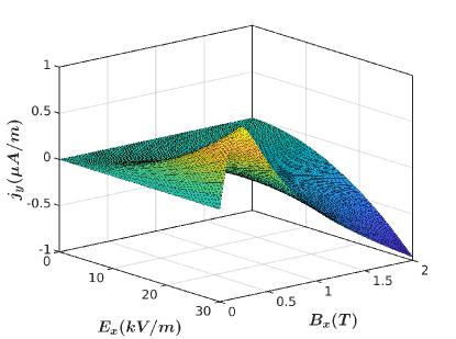
Figure 1: Non-linear anomalous Hall current density $\parallel\hat{\bm{y}}$ as a function of the in-plane magnetic field and of the driving electric field for a $30\,nm$ wide GaAs quantum well. The perpendicular Zeeman energy is $M=0.1$ meV.

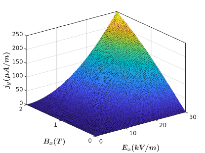
Figure 2: Non-linear anomalous Hall current density $\parallel\hat{\bm{y}}$ as a function of the in-plane magnetic field and of the driving electric field for a $30\,nm$ wide GaAs quantum well. The perpendicular Zeeman energy is $M=2$ meV.

In this work, we show that tetrahedral symmetry terms lead to a non-linear anomalous Hall effect in a symmetric hole quantum well. The effect occurs in the presence of both in-plane and out-of-plane Zeeman fields, the latter of which can be produced either by a small magnetic field or by magnetic impurities in a ferromagnetic semiconductor. The role of the $T_{d}$ terms can be understood as an electric-field induced shear term in the in-plane $g$-factor. Our main result is summarized in Figs. 1 and 2. We find a sizable non-linear anomalous Hall current density along the $y$-axis, accompanied by a much smaller non-linear longitudinal current density, not shown. The effect can be easily measured in readily available hole nanostructures, which provide a straightforward set-up for probing the existence of tetrahedral-symmetry terms. Based on realistic parameters we find that the non-linear anomalous Hall effect in spin-3/2 holes can be comparable in magnitude to the values reported recently in topological materials Kang et al. (2019). Aside from the novelty of identifying a non-linear electrical response purely due to holes, as opposed to well-known optical transitions linking the valence and conduction bands, a sizable tetrahedral contribution beyond the Luttinger model will have important repercussions for hole-based quantum computing, Nichele et al. (2014); Salfi et al. (2016a); Brauns et al. (2016a, b); Wang et al. (2016); Watzinger et al. (2016); Salfi et al. (2016b); Nichele et al. (2017); Srinivasan et al. (2017); Conesa-Boj et al. (2017); Li et al. (2017); Hung et al. (2017); Liles et al. (2018); Vukusic et al. (2018); Li et al. (2018); Crippa et al. (2018); Hendrickx et al. (2018, 2020) where it may enable additional possibilities for the electrical manipulation of holes.

Hamiltonian. We consider a symmetric hole quantum well grown in a zinc blende heterostructure along the high-symmetry crystallographic direction (001). The confinement is along the $z$-axis. For concreteness we consider GaAs with Luttinger parameters for $\gamma_{1}=6.85$, $\gamma_{2}=2.10$ and $\gamma_{3}=2.90$. The total Hamiltonian $H=H_{0}+U+H_{E}$ includes the band Hamiltonian, the disorder potential and the applied electric field. The band Hamiltonian is the combination of kinetic part and $H_{Z}$, $H_{0}=\hbar^{2}k^{2}/2m+H_{Z}$ where $H_{Z}$ is given by,

$$H_{Z}=\Delta_{1}B_{+}k_{+}^{2}\sigma_{-}+\Delta_{2}B_{-}k_{+}^{4}\sigma_{-}+\textbf{{h.c.}}+M\sigma_{3}$$ (1)

where $\Delta_{1}$ and $\Delta_{2}$ are the g-factors, $B_{\pm}=B_{x}\pm iB_{y}$ represent the in-plane magnetic field of magnitude $B_{\parallel}$, h.c. is Hermitian conjugate, $k_{\pm}=k_{x}\pm ik_{y}$, while $\sigma_{\pm}=(1/2)\,(\sigma_{x}\pm i\sigma_{y})$. Without loss of generality we set $B_{\parallel}=B_{x}$. We have denoted the Zeeman field in the $\hat{\bm{z}}$-direction by $M$, and define it so that $M$ has units of energy. The eigenvalues of $H_{0}$ are $\epsilon_{\bm{k}}^{(\pm)}=\epsilon_{k}^{(0)}\pm\Omega_{\bm{k}}$ where $\epsilon_{k}^{(0)}=\hbar^{2}k^{2}/2m$ is kinetic part and energy dispersion is split by $\Omega_{\bm{k}}=\sqrt{M^{2}+B_{\parallel}^{2}k^{4}G_{\bm{k}}}$, and $G_{\bm{k}}=(\Delta_{1})^{2}+k^{4}(\Delta_{2})^{2}+2k^{2}\Delta_{1}\Delta_{2}\cos(2\theta)$.

The two-by-two Hamiltonian given by $H_{0}$ is the projection of Luttinger Hamiltonian under Schrieffer-Wolff transformation to HH subspace, and the momentum-dependent $g$-factors reflect the strong spin-orbit interaction in Luttinger Hamiltonian Chow and Koch (1999); Winkler (2003). The interaction is known to be proportional to $B_{\parallel}k^{2}$, a term quadratic in in-plane momentum Winkler (2003) while recent work has identified a new term $B_{\parallel}k^{4}$ Miserev and Sushkov (2017) quartic in in-plane momentum, which has been confirmed experimentally Miserev et al. (2017). Such momentum-dependent Zeeman terms are specific to heavy holes, which represent the $\pm 3/2$ projection of the hole spin-$3/2$ onto the quantization axis. Note that, although the electric field is treated perturbatively, the Zeeman terms are treated exactly. The prefactors $\Delta_{1}$ and $\Delta_{2}$ are functions of $k$ and decrease strongly at larger wave vectors. Such terms are not present in spin-$1/2$ electron systems. In our evaluations this $k$-dependence is taken into account: we evaluate the coefficients for the specific carrier density we have chosen. The Zeeman interaction for heavy holes also includes terms $\propto B_{\parallel}^{3}$, yet these are three orders of magnitude smaller than the $B_{\parallel}-$linear terms above, only becoming important for $B_{\parallel}\geq 30$ T.

For a symmetric quantum well there is no Rashba spin-orbit interaction Winkler (2003); Moriya et al. (2014). Likewise, we have not included the Dresselhaus interaction in the Hamiltonian $H_{0}$ because it does not contribute to the non-linear signal: we have verified this explicitly. The interaction with a uniform electric field $\bm{E}$ makes two contributions to $H_{E}$, namely $H_{E}=e\bm{E}.\hat{\bm{r}}+H_{\lambda}$. The first is the customary electrostatic potential, while the second, denoted by $H_{\lambda}$, arises from $T_{d}$ symmetry, and has the form

$$H_{\lambda}=ie\lambda M(E_{+}k_{-}^{2}\sigma_{+}-E_{-}k_{+}^{2}\sigma_{-})$$ (2)

in which $E_{\pm}$ is the in-plane electric field, $M$ is the out-of-plane Zeeman field which we take to have units of energy, and $\lambda$ is a material-specific parameter whose magnitude will be determined below. We transform $H_{\lambda}$ to the eigenstate basis of $H_{0}$. Without loss of generality we assume that the electric field points in the $\hat{\bm{x}}$ direction, yielding $\tilde{H}_{\lambda}=eE_{x}k^{2}M\lambda\tilde{\sigma}_{y}$, where the tilde indicates matrices in the eigenstate basis, hence $\tilde{\sigma}_{y}$ is a pseudospin rather than a spin matrix. By comparing $H_{\lambda}$ and $H_{Z}$ we note that $H_{\lambda}$ can be understood as an electric-field correction to the Zeeman Hamiltonian: $T_{d}$-symmetry mixes the out-of-plane Zeeman field with the in-plane electric field, yielding an additional in-plane Zeeman interaction. This is essentially an electrically tunable shear term in the $g$-tensor. An analogous correction is present for the out-of-plane Zeeman interaction due to an out-of-plane electric field and an in-plane Zeeman field, as discussed in the Supplement.

Figure 3: The non-linear anomalous Hall effect is a non-monotonic function of the in-plane magnetic field, shown here for two different values of the out-of-plane Zeeman field: $M=2$ meV and $M=0.1$ meV. The electric field is $E_{x}=30\,kV/m$.

Kinetic equation. The quantum Liouville equation for first order in electric field is given by,

$$\frac{\partial\rho_{E}}{\partial t}+\frac{i}{\hbar}[H_{0},\langle\rho_{E}\rangle]+J(\langle\rho_{E}\rangle)=-\frac{i}{\hbar}[H_{E},\langle\rho_{0}\rangle]$$ (3)

where $\rho_{0}$ and $\rho_{E}$ are the equilibrium and first-order response density matrices. Scattering term in the Born approximation is written as $J(\langle\rho\rangle)=\frac{1}{\hbar^{2}}\int_{0}^{\infty}dt^{\prime}\langle[U,[e^{-iH_{0}t^{\prime}/\hbar}Ue^{iH_{0}t^{\prime}/\hbar},\langle\rho(t)\rangle]]\rangle$. We assume that the disorder potential is given by a short-range disorder $U(\bm{r})=U_{0}\sum_{i}\delta(\bm{r}-\bm{r}_{i})$ and the correlation function yields us $\langle U(\bm{r})U(\bm{r}^{\prime})\rangle=n_{i}U_{0}^{2}\,\delta(\bm{r}-\bm{r}^{\prime})$ with $n_{i}$ the impurity density. The driving term has two contributions,

$$D_{E\bm{k}}=\frac{eE_{x}}{\hbar}\bigg{\{}\frac{\partial\rho_{0}}{\partial k_{x}}-i\left[\mathcal{R}_{k_{x}},\rho_{0}\right]\bigg{\}}-\frac{i}{\hbar}[\tilde{H}_{\lambda},\rho_{0}]$$ (4)

in which $\mathcal{R}_{k_{x}}=\langle u_{\bm{k}}|\left(i\partial u_{\bm{k}}/\partial k_{x}\right)\rangle$ is the Berry connection. In the crystal momentum representation, i.e. $|m,\bm{k}\rangle=e^{i\bm{k}.\bm{r}}|u_{m\bm{k}}\rangle$, the equilibrium density matrix is simply Fermi-Dirac distribution function given at energy $\epsilon_{\bm{k}}^{(m)}$, $\langle m,\bm{k}|\langle\rho_{0}\rangle|m^{\prime},\bm{k}\rangle=f_{0}(\epsilon_{\bm{k}}^{(m)})\delta^{mm^{\prime}}$. The eigenstates are evaluated in the absence of the electric field. The terms in the curly brackets are the consequences of $e\bm{E}.\hat{\bm{r}}$. The first term in curly bracket is the Fermi surface response. The second term in curly bracket and the term outside the curly bracket contains Fermi sea responses.

To determine the density matrix response $\rho_{E}$ we solve equation 3 up until a linear order of the electric field. Using the same differential equation we try to find the second-order density matrix responses but this time we solve the equation followed by these substitutions, $\rho_{0}\rightarrow\rho_{E}$ and $\rho_{E}\rightarrow\rho_{E2}$. Having access to driving term we can derive the diagonal and off-diagonal parts of the density matrix Culcer et al. (2017). The off-diagonal part of the density matrix $\rho_{E}$ can be calculated using the off-diagonal terms in the driving term (Eq. 4, refer to appendix). Accordingly, the band-diagonal part of the density matrix is given by

$$J_{d}[(n_{E})^{(-1)}]^{mm}=\frac{e\bm{E}}{\hbar}\cdot\frac{\partial f_{0}(\epsilon_{\bm{k}}^{(m)})}{\partial\bm{k}}$$ (5)

where $\partial f_{0}(\epsilon_{\bm{k}}^{(m)})/\partial\epsilon_{\bm{k}}^{(m)}\approx-\delta[\epsilon_{\bm{k}}^{(m)}-\epsilon_{F}]$ at low temperatures, with $\epsilon_{F}$ the Fermi energy.

Second-order electrical response. We analytically derive the conductivity with $\Delta_{2}$ set to zero. For pedagogical purposes we perform an analytical calculation first, using a simplified model. $G_{\bm{k}}$ becomes simply $\Delta_{1}^{2}$ if we neglect $\Delta_{2}$. The term $\Omega_{\bm{k}}$ is function of both $k$ and $\theta$ if we take into account both g-factors. But if we only consider one of the $g$-factors the dispersion is isotropic. Hence, the overall calculation becomes much simpler if we only consider one of the $g$-factors. To second order we find $j_{x}=\chi_{xxx}E_{x}^{2}$ and $j_{y}=\chi_{yxx}E_{x}^{2}$, where

$$\chi_{xxx}=\frac{2e^{3}B_{x}^{3}\Delta_{1}^{3}k_{F}^{6}mM^{2}\lambda}{\pi\hbar^{3}\Omega_{F}^{4}}$$

$$\chi_{yxx}=\frac{2e^{3}\lambda mM\tau B_{x}\Delta_{1}k_{F}^{2}\left(\Omega_{F}^{2}+M^{2}\right)}{\pi\hbar^{4}\Omega_{F}^{2}},$$ (6)

where $\Omega_{F}=\sqrt{M^{2}+B_{x}^{2}\Delta_{1}^{2}k_{F}^{4}}$, $k_{F}$ is the Fermi wave vector, and the momentum relaxation time $\tau=\hbar^{3}/(n_{i}U^{2}m)$. Numerically we extend our results for the general case while $\Delta_{2}$ effect is taken into account. The transverse non-linear current density, shown in Figs. 1 - 4, is larger than its longitudinal counterpart (not shown) by several orders of magnitude. In both cases, in the presence of $\Delta_{2}$, the behavior of the current density is non-monotonic in terms of the magnetic field but in general $|j_{y}|$ increases linearly in terms of the magnetic field while the magnetic field is larger compared to magnetization. As we expect, the current density in second-order behaves as an increasing parabolic function in terms of electric field (Fig. 1 - 2). In Fig. 4 we can see that in the range of values set for magnetic and electric field, the current density behaves almost linearly as a function of magnetization.

To obtain $\lambda$, we start from the Luttinger Hamiltonian combined with the electric-dipole and Zeeman Hamiltonians, and we apply the Schrieffer-Wolff transformation to project the system to the HH subspace. This yields an effective $2\times 2$ Hamiltonian of the same form as $H_{0}$. In the axial approximation $\lambda=(3a_{B}\xi)/(8\bar{\gamma}\langle k_{z}^{2}\rangle^{2}\mu)$, in which $a_{B}$ is the Bohr radius, and $\xi$ is a parameter controlling the intensity of electric-dipole terms. Due to the confinement along the $z$-axis we know that $k_{z}$ is comparatively larger than in-plane wave vectors Winkler et al. (2008). For the following values, $\xi=0.2,\mu=\hbar^{2}/m_{0}\;(m_{0}\,\text{is the bare electron mass}),\bar{\gamma}=2.5,k_{z}=(\pi/30\;nm)$, we obtain $\lambda=1.08\times 10^{-6}{\rm ms^{2}kg^{-1}}$.

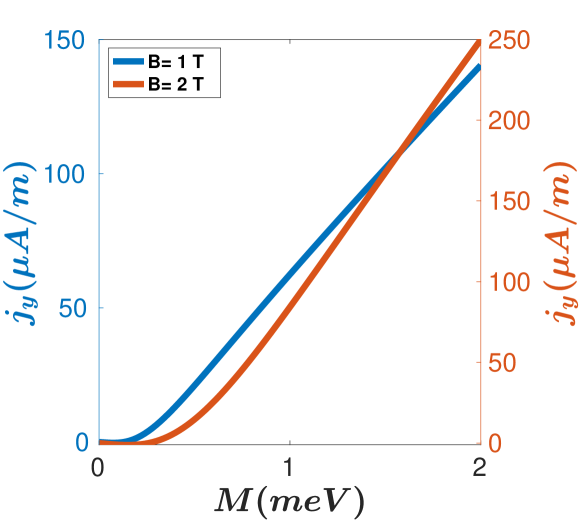
Figure 4: Non-linear anomalous Hall current under the considered range of values for the parameters in current densities behave approximately linearly in terms of magnetization ($M$). Electric field is considered as $E_{x}=30\,kV/m$.

Discussion. The conductivities that we calculated in the second-order response are directly proportional to $\lambda$. We found that $\lambda$ is proportional to the size of quantum well. Therefore, this effect will be pronounced in larger wells. Furthermore, it is easy to see that the second-order response thoroughly is dependent on $\xi$, meaning that at $\xi=0$ (for crystals with a center of inversion symmetry) the second-order response vanishes. Marcellina et al. Marcellina et al. (2020) shows that in spin-3/2 system with two different $g$-factors (each have different winding numbers) there appears a sizable anisotropy in conductivities and Hall coefficient. We have shown that in the similar system a sizable nonlinear response can be probed using $H_{\lambda}$ (Eq. 2). Note that, although the non-linear anomalous Hall effect is stronger in higher mobility systems, the ratio $j^{(2)}/\sigma_{xx}$ is independent of the mobility, playing the role of a nonlinear Hall coefficient.

In the absence of $\Delta_{2}$ the absolute value of the current density increases monotonically as a function of the out-of-plane Zeeman energy and in-plane magnetic field. When either quantity, i.e. $M$ or $B_{x}$, reaches a sizable value $|j_{y}|$ becomes essentially linear in that quantity. On the other hand, when $\Delta_{2}$, which has a different sign from $\Delta_{1}$, is accounted for in the Hamiltonian, $|j_{y}|$ is non-monotonic as a function of $B_{x}$ in the range of $M(meV)\in[0,2]$ but it still behaves monotonically as a function of $M$ in the range of $B_{x}(T)\in[0,2]$. Nevertheless, the current density behaves linearly at comparatively large (small) values of $M$ and small (large) values of $B_{x}$. One can also see from figure 3 that the first derivative of $j_{y}$ changes sign depending on the size of the magnetization.

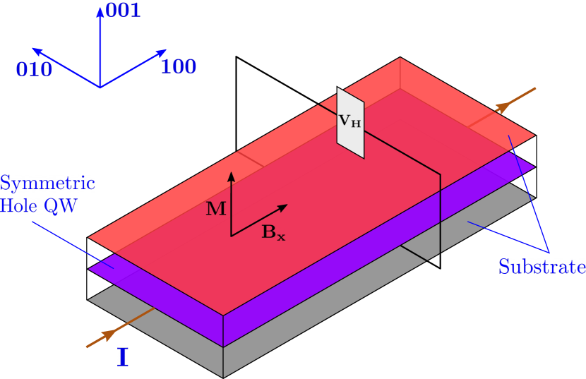
Figure 5: Schematic of one potential experimental setup involving a symmetric hole quantum well. The effect can be detected by measuring the Hall voltage.

Experimental observation. There is considerable flexibility in regard to experimental observation, with one possibility illustrated in Fig. 5. To detect a signal of second order in the applied electric field one requires a low-frequency alternating field, which can be accomplished using an oscillator with a frequency of the order of $\omega/(2\pi)\sim 100$ Hz. The Hall voltage at $2\omega$ can then be read out. The relaxation time $\tau$ in general is much smaller than the alternating electric field time period, i.e. $\omega\tau\ll 1$, hence our DC calculation is appropriate to describe this physics. The key feature is the way the perpendicular Zeeman field is generated: this can be accomplished either via a magnetic doping, as in ferromagnetic semiconductors, or by applying a perpendicular magnetic field. We discuss each in turn. To facilitate comparison with nonlinear effects in topological materials we will use the exact sample size used in Ref. Kang et al., 2019

The easiest way is using an unmagnetized GaAs sample together with a vector magnet generating an arbitrary magnetic field. The out-of-plane magnetic field can be set so that the Zeeman energy is $M\approx 0.1$ meV so that one can neglect the orbital terms giving rise to the ordinary linear Hall effect, even though these do not contribute to the non-linear anomalous Hall voltage. To determine the Hall voltage we start with the relationship between the resistivity and conductivity tensors

$$\left(\begin{array}[]{cc}\rho_{xx}&\rho_{xy}\\ \rho_{yx}&\rho_{yy}\\ \end{array}\right)=\frac{1}{\sigma_{xx}^{2}+\sigma_{yx}^{2}}\left(\begin{array}[]{cc}\sigma_{xx}&-\sigma_{xy}\\ \sigma_{xy}&\sigma_{xx}\\ \end{array}\right).$$ (7)

The induced non-linear Hall electric field takes the form

$$E_{y}^{(2)}\approx\frac{\chi_{yxx}}{\sigma_{xx}}E_{x}^{2},$$ (8)

as outlined in the Supplement. Assuming $M=0.1$ meV, using figure 1 we take the current density $0.96\,\mu A/m$ corresponding to the magnetic field, electric field, and magnetization provided at $B_{x}=2\,T$, $E_{x}=30\,kV/m$, and $M=0.1\,meV$. To find the conductivity we consider that a relaxation time $\tau=1$ ps. The hole carriers density is taken to be $1.86\times 10^{15}\,m^{-2}$. The heavy hole in-plane mass is $m^{*}=m_{0}/(\gamma_{1}+\bar{\gamma})$, yielding

$$\sigma_{xx}=\frac{ne^{2}\tau}{m^{*}}\approx 12.7\,\frac{e^{2}}{h},$$ (9)

hence the induced non-linear Hall electric field $E_{y}^{(2)}\approx 2\times 10^{-3}$ V/m and a corresponding non-linear Hall voltage $V_{y}^{(2)}=E_{y}^{(2)}d=18$ nV.

A class of state-of-art samples that can be used to study nonlinear effects are magnetic semiconductors, such as GaMnAs Ohno et al. (1999, 2000); Fukumura et al. (2001); Tang et al. (2004); Gould et al. (2004); Rüster et al. (2003); Giddings et al. (2005); Krainov et al. (2021). The magnetization easy axis in GaMnAs can be either in the plane or out of the plane Lee et al. (2009), and the orientation can be tailored by means of strain. We focus on the latter case in this example and assume a larger value of $M\approx 2$ meV. From figure 2 we take the current density to be 0.25 mA/m corresponding to a magnetic field and electric field of $B_{x}=2\,T$ and E = 30 kV/m respectively. Using the same carrier density and relaxation time as above we find the same value for $\sigma_{xx}$, whereupon the induced non-linear Hall electric field $E_{y}^{(2)}\approx 0.5$ V/m, and, in a sample of width $9.2\,\mu m$ as in Kang et al. (2019), we find a Hall voltage $V_{y}^{(2)}\approx 5\,\mu$V, which is comparable in size to Ref. Kang et al., 2019.

In summary, we have demonstrated that in a symmetric quasi-2D hole system a sizable non-linear anomalous Hall effect is present, driven by tetrahedral symmetry terms that go beyond the Luttinger model. The effect is measurable either in a conventional GaAs sample using a vector magnet, or in a sample of ferromagnetic GaAs in a magnetic field, where the magnetic field orientation is chosen depending on the direction of the magnetization.

Appendix A Appendix A: Basis states and scattering term

The eigenvector of $H_{0}=h^{2}k^{2}/2m+H_{Z}$ are calculated as,

$$u_{\bm{k}}^{(\pm)}=\sqrt{\frac{\Omega_{\bm{k}}\mp M}{2\Omega_{\bm{k}}}}\left(\begin{array}[]{c}\frac{e^{-2i\theta}\left(M\pm\Omega_{\bm{k}}\right)}{Bk^{2}\left(\Delta_{1}+e^{2i\theta}k^{2}\Delta_{2}\right)}\\ 1\\ \end{array}\right)$$ (12)

where $\Omega_{\bm{k}}=\sqrt{M^{2}+B_{\parallel}^{2}k^{4}G_{\bm{k}}}$, and $G_{\bm{k}}=(\Delta_{1})^{2}+k^{4}(\Delta_{2})^{2}+2k^{2}\Delta_{1}\Delta_{2}\cos(2\theta)$, while $\theta=\tan^{-1}\left(k_{y}/k_{x}\right)$.

Since $H_{\lambda}$ is linear in the electric field, in addition to $e\bm{E}.\hat{\bm{r}}$, we need to add this term to driving term (Eq. 4) too. To do so, We have to transform $H_{\lambda}$ using S matrix which is formed based on $H_{0}$ eigenvectors.

$$\tilde{H}_{\lambda}=S^{\dagger}H_{\lambda}S$$ (13)

where

$$S=\begin{pmatrix}u_{\bm{k}}^{(1)}(1,1)&u_{\bm{k}}^{(2)}(1,1)\\ u_{\bm{k}}^{(1)}(2,1)&u_{\bm{k}}^{(2)}(2,1)\end{pmatrix}.$$ (14)

here $u_{\bm{k}}^{(1)}$, and $u_{\bm{k}}^{(2)}$ correspond to $u_{\bm{k}}^{(-)}$, and $u_{\bm{k}}^{(+)}$ (Eq. 12), respectively. Another parameter that we have used in driving term is the x-component of Berry connection (Eq. 4). While $\Delta_{2}=0$, we find the Berry connection’s x-component using the eigenvectors that we have calculated recently,

$$\mathcal{R}_{k_{x}}=\bigg{\langle}u_{\bm{k}}\bigg{\rvert}i\frac{\partial u_{\bm{k}}}{\partial k_{x}}\bigg{\rangle}=-\frac{\sin(\theta)}{k}\sigma_{0}+\frac{M\sin(\theta)}{k\Omega_{k}}\sigma_{3}+\frac{B\Delta_{1}k\sin(\theta)}{\Omega_{k}}\sigma_{1}-\frac{B\Delta_{1}Mk\cos(\theta)}{\Omega_{k}^{2}}\sigma_{2}.$$ (15)

here, $\Omega_{k}$ is isotropic since $\Delta_{2}$ is considered to be zero.
 
Off-diagonal part of the density matrix in linear and later in the second-order response can be derived using equation 3. Taking only the off-diagonal terms from both sides of equation 3 leads us to

$$\frac{\partial S_{E\bm{k}}}{\partial t}+\frac{i}{\hbar}\left[H_{0},S_{E\bm{k}}\right]=D_{E\bm{k}}+D^{\prime}_{E\bm{k}}$$ (16)

Comparing both sides of equation 16 and using equation 4 we can write,

$$S_{E\bm{k}}^{mm^{\prime}}=-i\hbar\mathcal{P}\left(\frac{D_{E\bm{k}}^{mm^{\prime}}+D_{E\bm{k}}^{\prime mm^{\prime}}}{\epsilon_{\bm{k}}^{m}-\epsilon_{\bm{k}}^{m^{\prime}}}\right)$$ (17)

while $D^{\prime}_{E\bm{k}}=-J_{od}\left[n_{E\bm{k}}\right]$ (for further details please refer to Culcer et al. (2017)). Off-diagonal part of density matrix takes a linear form in terms of electric field in linear response. In the case that $\Delta_{2}$ is set to zero we get for $S_{E\bm{k}}$,

$$S_{E\bm{k}}=\frac{eE_{x}kB\Delta_{1}\sin(\theta)}{2\Omega_{k}^{2}}\left(-f_{1}+f_{2}\right)(\sigma_{1})-\frac{eE_{x}kM(-B\cos(\theta)\Delta_{1}+k\lambda\Omega_{k}^{2})}{2\Omega_{k}^{3}}\left(-f_{1}+f_{2}\right)(\sigma_{2})$$ (18)

here $f_{1}$ and $f_{2}$ are Fermi-Dirac distribution function given at energies $\epsilon_{\bm{k}}^{(1)}$, and $\epsilon_{\bm{k}}^{(2)}$, respectively. $\Omega_{k}$ has no angular dependency, i.e., $\Omega_{k}=\sqrt{M^{2}+B^{2}\Delta_{1}^{2}k^{4}}$. In our calculations, we see that $D_{E\bm{k}}^{\prime mm^{\prime}}$ contribution to $S_{E\bm{k}}$ is zero. To get the diagonal part of the density matrix ($n_{E\bm{k}}=n_{E\bm{k}}^{(0)}\sigma_{0}+n_{E\bm{k}}^{(\Omega)}\sigma_{3}$), we need to solve equation 5 along with the following equation 19

$$[J_{d}(n)]_{\bm{k}}^{mm}=\frac{2\pi n_{i}}{\hbar}\sum_{m^{\prime}\bm{k}^{\prime}}U_{\bm{k}\bm{k}^{\prime}}^{mm^{\prime}}U_{\bm{k}^{\prime}\bm{k}}^{m^{\prime}m}(n_{E\bm{k}}^{mm}-n_{E\bm{k}^{\prime}}^{m^{\prime}m^{\prime}})\delta(\epsilon_{\bm{k}}^{m}-\epsilon_{\bm{k}^{\prime}}^{m^{\prime}})$$ (19)

which leads to

$$[J_{0}(n_{E\bm{k}}^{(0)})]^{(1,1)}=[D_{0}]^{(1,1)}$$ (20)

$$[J_{0}(n_{E\bm{k}}^{(\Omega)})]^{(1,1)}=[D_{\Omega}]^{(1,1)}-[J_{\Omega}(n_{E\bm{k}}^{(0)})]^{(1,1)}$$ (21)

here, we assume that the diagonal part of driving term is $D^{(d)}_{E\bm{k}}=D_{0}\sigma_{0}+D_{\Omega}\sigma_{\Omega}$. Thus, $\Delta_{2}=0$ yields us,

$$n_{E\bm{k}}^{(0)} =-\frac{\hbar eE_{x}}{m}\tau k\cos(\theta)\delta\left(\epsilon_{k}^{(0)}-\epsilon_{F}\right)$$

$$n_{E\bm{k}}^{(\Omega)} =\frac{\tau eE_{x}}{\hbar}\cos(\theta)\bigg{(}\frac{\hbar^{2}k}{m}\bigg{)}\left(\Omega_{k}\frac{\partial}{\partial\epsilon_{k}^{(0)}}\delta(\epsilon_{k}^{(0)}-\epsilon_{F})\right)+\frac{\tau eE_{x}}{\hbar}\cos(\theta)\bigg{(}\frac{2B^{2}k^{3}\Delta_{1}^{2}}{\Omega_{k}}\bigg{)}\delta\left(\epsilon_{k}^{(0)}-\epsilon_{F}\right)$$ (22)

and $\tau=\frac{\hbar^{3}}{n_{i}U^{2}m}$ is the relaxation time. The disorder potential matrix elements in equation 19 are given by,

$$U_{\bm{k},\bm{k}^{\prime}}{}^{(m,m^{\prime})}=\langle m,\bm{k}|U|m^{\prime},\bm{k}^{\prime}\rangle$$ (23)

$$U_{\bm{k},\bm{k}^{\prime}}{}^{(1,1)}=\frac{U}{2\sqrt{\Omega_{k}\Omega_{k^{\prime}}}}\left(e^{+2i(\theta-\theta^{\prime})}\sqrt{\Omega_{k}-M}\sqrt{\Omega_{k^{\prime}}-M}+\sqrt{\Omega_{k}+M}\sqrt{\Omega_{k^{\prime}}+M}\right)$$ (24)

$$U_{\bm{k}^{\prime},\bm{k}}{}^{(1,1)}=\langle 1,\bm{k}^{\prime}|U|1,\bm{k}\rangle=U\langle 1,\bm{k}^{\prime}|1,\bm{k}\rangle=(U\langle 1,\bm{k}|1,\bm{k}^{\prime}\rangle)^{\dagger}=\left(U_{\bm{k},\bm{k}^{\prime}}{}^{(1,1)}\right)^{\dagger}$$ (25)

$$U_{\bm{k},\bm{k}^{\prime}}{}^{(1,2)}=\frac{U}{2\sqrt{\Omega_{k}\Omega_{k^{\prime}}}}\left(-e^{2i(\theta-\theta^{\prime})}\sqrt{\Omega_{k}-M}\sqrt{\Omega_{k^{\prime}}+M}+\sqrt{\Omega_{k}+M}\sqrt{\Omega_{k^{\prime}}-M}\right)$$ (26)

$$U_{\bm{k}^{\prime},\bm{k}}{}^{(2,1)}=\langle 2,\bm{k}^{\prime}|U|1,\bm{k}\rangle=U\langle 2,\bm{k}^{\prime}|1,\bm{k}\rangle=[U\langle 1,\bm{k}|2,\bm{k}^{\prime}\rangle]^{\dagger}=\left(U_{\bm{k},\bm{k}^{\prime}}{}^{(1,2)}\right)^{\dagger}$$ (27)

$$\begin{split}&|U_{\bm{k},\bm{k}^{\prime}}{}^{(1,1)}|^{2}+|U_{\bm{k},\bm{k}^{\prime}}{}^{(1,2)}|^{2}=U^{2}\end{split}$$ (28)

$$\begin{split}&-|U_{\bm{k},\bm{k}^{\prime}}{}^{(1,1)}|^{2}+|U_{\bm{k},\bm{k}^{\prime}}{}^{(1,2)}|^{2}=\frac{U^{2}}{4\Omega_{k}\Omega_{k^{\prime}}}\bigg{\{}-4M^{2}-2\left(\sqrt{\Omega_{k}+M}\sqrt{\Omega_{k}-M}\sqrt{\Omega_{k^{\prime}}+M}\sqrt{\Omega_{k^{\prime}}-M}\right)\\ &\left[e^{2i(\theta-\theta^{\prime})}+e^{-2i(\theta-\theta^{\prime})}\right]\bigg{\}}\end{split}$$ (29)

$$U_{\bm{k},\bm{k}^{\prime}}{}^{(2,2)}=\frac{U}{2\sqrt{\Omega_{k}\Omega_{k^{\prime}}}}\left(e^{2i(\theta-\theta^{\prime})}\sqrt{\Omega_{k}+M}\sqrt{\Omega_{k^{\prime}}+M}+\sqrt{\Omega_{k}-M}\sqrt{\Omega_{k^{\prime}}-M}\right)$$ (30)

$$U_{\bm{k}^{\prime},\bm{k}}{}^{(2,2)}=\langle 2,\bm{k}^{\prime}|U|2,\bm{k}\rangle=U\langle 2,\bm{k}^{\prime}|2,\bm{k}\rangle=(U\langle 2,\bm{k}|2,\bm{k}^{\prime}\rangle)^{\dagger}=(U_{\bm{k},\bm{k}^{\prime}}{}^{(2,2)})^{\dagger}$$ (31)

$$U_{\bm{k},\bm{k}^{\prime}}{}^{(2,1)}=\frac{U}{2\sqrt{\Omega_{k}\Omega_{k^{\prime}}}}\left(-e^{2i\left(\theta-\theta^{\prime}\right)}\sqrt{\Omega_{k}+M}\sqrt{\Omega_{k^{\prime}}-M}+\sqrt{\Omega_{k}-M}\sqrt{\Omega_{k^{\prime}}+M}\right)$$ (32)

$$U_{\bm{k}^{\prime},\bm{k}}{}^{(1,2)}=\langle 1,\bm{k}^{\prime}|U|2,\bm{k}\rangle=U\langle 1,\bm{k}^{\prime}|2,\bm{k}\rangle=\left(U\langle 2,\bm{k}|1,\bm{k}^{\prime}\rangle\right)^{\dagger}=\left(U_{\bm{k},\bm{k}^{\prime}}{}^{(2,1)}\right)^{\dagger}$$ (33)

$$\begin{split}&|U_{\bm{k},\bm{k}^{\prime}}{}^{(2,1)}|^{2}+|U_{\bm{k},\bm{k}^{\prime}}{}^{(2,2)}|^{2}=U^{2}\end{split}$$ (34)

$$\begin{split}-|U_{\bm{k},\bm{k}^{\prime}}{}^{(2,1)}|^{2}+|U_{\bm{k},\bm{k}^{\prime}}{}^{(2,2)}|^{2}=\frac{U^{2}}{4\Omega_{k}\Omega_{k^{\prime}}}\bigg{\{}4M^{2}+\left(2\sqrt{\Omega_{k}+M}\sqrt{\Omega_{k}-M}\sqrt{\Omega_{k^{\prime}}+M}\sqrt{\Omega_{k^{\prime}}-M}\right)\left[e^{2i(\theta-\theta^{\prime})}+e^{-2i(\theta-\theta^{\prime})}\right]\bigg{\}}\end{split}$$ (35)

Delta functions can be Taylor expanded in terms of pure kinetic parts and split energies,

$$\delta\left(\epsilon_{\bm{k}}^{(1)}-\epsilon_{\bm{k}^{\prime}}^{(1)}\right)=\delta\left(\epsilon_{k}^{(0)}-\epsilon_{k^{\prime}}^{(0)}\right)-(\Omega_{\bm{k}}-\Omega_{\bm{k^{\prime}}})\frac{\partial}{\partial\epsilon_{k}^{(0)}}\delta\left(\epsilon_{k}^{(0)}-\epsilon_{k^{\prime}}^{(0)}\right)$$

$$\delta\left(\epsilon_{\bm{k}}^{(1)}-\epsilon_{\bm{k}^{\prime}}^{(2)}\right)=\delta\left(\epsilon_{k}^{(0)}-\epsilon_{k^{\prime}}^{(0)}\right)-(\Omega_{\bm{k}}+\Omega_{\bm{k^{\prime}}})\frac{\partial}{\partial\epsilon_{k}^{(0)}}\delta\left(\epsilon_{k}^{(0)}-\epsilon_{k^{\prime}}^{(0)}\right)$$

$$\delta\left(\epsilon_{\bm{k}}^{(2)}-\epsilon_{\bm{k}^{\prime}}^{(1)}\right)=\delta\left(\epsilon_{k}^{(0)}-\epsilon_{k^{\prime}}^{(0)}\right)+(\Omega_{\bm{k}}+\Omega_{\bm{k^{\prime}}})\frac{\partial}{\partial\epsilon_{k}^{(0)}}\delta\left(\epsilon_{k}^{(0)}-\epsilon_{k^{\prime}}^{(0)}\right)$$

$$\delta\left(\epsilon_{\bm{k}}^{(2)}-\epsilon_{\bm{k}^{\prime}}^{(2)}\right)=\delta\left(\epsilon_{k}^{(0)}-\epsilon_{k^{\prime}}^{(0)}\right)+(\Omega_{\bm{k}}-\Omega_{\bm{k^{\prime}}})\frac{\partial}{\partial\epsilon_{k}^{(0)}}\delta\left(\epsilon_{k}^{(0)}-\epsilon_{k^{\prime}}^{(0)}\right)$$ (36)

Across our calculations we have used widely the following properties.

$$\delta\left(\epsilon_{k}^{(0)}-\epsilon_{F}\right)=\frac{\delta\left(k-k_{F}\right)}{\frac{\hbar^{2}k_{F}}{m}}$$ (37)

$$\frac{\partial}{\partial\epsilon_{k}^{(0)}}=\frac{1}{\frac{\hbar^{2}k}{m}}\frac{\partial}{\partial k}$$ (38)

$$k_{x}=k_{x}(k,\theta),\quad k_{y}=k_{y}(k,\theta)$$ (39)

$$\frac{\partial}{\partial k_{x}}=\cos(\theta)\frac{\partial}{\partial k}-\frac{1}{k}\sin(\theta)\frac{\partial}{\partial\theta}$$ (40)

$$\frac{\partial}{\partial k_{y}}=\sin(\theta)\frac{\partial}{\partial k}+\frac{1}{k}\cos(\theta)\frac{\partial}{\partial\theta}$$ (41)

Appendix B Appendix B: Second order response

Driving term in the second order is given by,

$$D_{E2}=\frac{eE_{x}}{\hbar}\left(\frac{\partial\rho_{E}}{\partial k_{x}}-i[\mathcal{R}_{k_{x}},\rho_{E}]\right)-\frac{i}{\hbar}\left[\tilde{H}_{\lambda},\rho_{E}\right]$$ (42)

in which $\rho_{E}$ is the density matrix derived in linear response. Here we carry out very similar calculations as we carried on in the linear response to find out $\rho_{E2}$ the second-order density matrix response. Replacing $\rho_{E}$ by $\rho_{0}$ in equation 3 and renaming $\rho_{E}$ to $\rho_{E2}$, we can work and find again the diagonal and off-diagonal parts of $\rho_{E2}=n_{E2}+S_{E2}$. The off-diagonal part of $\rho_{E2}$ can be calculated using equation 17 in the following form,

$$S_{E2} =S_{E2}^{(1)}\sigma_{1}+S_{E2}^{(2)}\sigma_{2}$$ (43)

We find the $S_{E2}$ in terms of $\sigma_{1}$ and $\sigma_{2}$,

$$S_{E2}=\frac{eE_{x}}{4\Omega^{6}}\Big{\{}-eE_{x}k\lambda M\Omega_{k}^{2}\cos(\theta)\left[2B^{2}\Delta_{1}^{2}k^{4}-\Omega_{k}^{2}(2+k\partial_{k})\right](f_{1}-f_{2})$$

$$+eE_{x}B\Delta_{1}M\cos^{2}(\theta)\left[6B^{2}\Delta_{1}^{2}k^{4}-\Omega_{k}^{2}(1+k\partial_{k})\right](f_{1}-f_{2})+B\Delta_{1}\Omega_{k}^{2}\sin(\theta)\left[eE_{x}M(f_{1}-f_{2})\sin(\theta)-4kn_{\Omega}\Omega_{k}^{2}\right]\Big{\}}\sigma_{1}$$

$$+\frac{eE_{x}}{4\Omega_{k}^{5}}\Big{\{}2k\lambda M\Omega_{k}^{2}\left[eE_{x}M(f_{1}-f_{2})\sin(\theta)-2kn_{\Omega}\Omega_{k}^{2}\right]$$

$$+B\Delta_{1}\cos(\theta)\left[4kMn_{\Omega}\Omega_{k}^{2}-eE_{x}\sin(\theta)\left(-4B^{2}\Delta_{1}^{2}k^{4}+2M^{2}+k\Omega_{k}^{2}\partial_{k}\right)(f_{1}-f_{2})\right]\Big{\}}\sigma_{2}.$$ (44)

where $n_{\Omega}$ is given at equation 22. The diagonal parts of $\rho_{E2}$ becomes,

$$n_{E2}=n_{E2}^{(0)}\sigma_{0}+n_{E2}^{(\Omega)}\sigma_{3}$$ (45)

$$n_{E2}^{(0)}= -\frac{e^{2}E_{x}^{2}}{m}\tau^{2}\delta(\epsilon_{k}^{(0)}-\epsilon_{F})-\frac{e^{2}E_{x}^{2}}{m}\tau^{2}k\cos^{2}(\theta)\frac{\partial}{\partial k}\delta(\epsilon_{k}^{(0)}-\epsilon_{F})$$ (46)

$$n_{E2}^{(\Omega)} =\frac{2e^{2}E_{x}^{2}(M^{2}+\Omega_{k}^{2})\tau^{2}}{k^{2}\hbar^{2}\Omega_{k}}\delta(\epsilon_{k}^{(0)}-\epsilon_{F})+\frac{e^{2}E_{x}^{2}\Omega_{k}(-7M^{2}+8\Omega_{k}^{2})\tau^{2}}{2k\hbar^{2}(-M^{2}+\Omega_{k}^{2})}\frac{\partial}{\partial k}\delta(\epsilon_{k}^{(0)}-\epsilon_{F})$$

$$+\frac{e^{2}E_{x}^{2}\Omega_{k}(-2M^{2}+4\Omega_{k}^{2})\tau^{2}}{4\hbar^{2}(-M^{2}+\Omega_{k}^{2})}\frac{\partial}{\partial k}\frac{\partial}{\partial k}\delta(\epsilon_{k}^{(0)}-\epsilon_{F})+\frac{4e^{2}E_{x}^{2}M^{2}(-M^{2}+\Omega_{k}^{2})\cos(2\theta)\tau^{2}}{k^{2}\hbar^{2}\Omega_{k}(M^{2}+\Omega^{2})}\delta(\epsilon_{k}^{(0)}-\epsilon_{F})$$

$$+\frac{e^{2}E_{x}^{2}\Omega_{k}(-5M^{2}+3\Omega_{k}^{2})\cos(2\theta)\tau^{2}}{2k\hbar^{2}(M^{2}+\Omega_{k}^{2})}\frac{\partial}{\partial k}\delta(\epsilon_{k}^{(0)}-\epsilon_{F})+\frac{e^{2}E_{x}^{2}\Omega_{k}\cos(2\theta)\tau^{2}}{2\hbar^{2}}\frac{\partial}{\partial k}\frac{\partial}{\partial k}\delta(\epsilon_{k}^{(0)}-\epsilon_{F})$$ (47)

Density matrix can be expressed in terms of diagonal and off-diagonal terms, $\rho_{E2}=n_{E2}+S_{E2}$.

$$\text{tr}(v_{x}\rho_{E2})=\text{tr}\left[v_{x}^{(d)}n_{E2}\right]+\text{tr}\left[v_{x}^{(od)}S_{E2}\right]$$

$$\text{tr}(v_{y}\rho_{E2})=\text{tr}\left[v_{y}^{(d)}n_{E2}\right]+\text{tr}\left[v_{y}^{(od)}S_{E2}\right]$$ (48)

where $(d)$ and $(od)$ denotes the diagonal and off-diagonal parts of the velocity matrices along x and y directions. Diagonal parts of velocities at $\Delta_{2}=0$ are given by,

$$v_{x}^{(d)}=\frac{1}{\hbar}\left(\begin{array}[]{cc}\frac{\partial\epsilon_{k}^{(1)}}{\partial k_{x}}&0\\ 0&\frac{\partial\epsilon_{k}^{(2)}}{\partial k_{x}}\\ \end{array}\right)=\frac{1}{\hbar}\frac{\hbar^{2}k}{m}\cos(\theta)\sigma_{0}-\frac{1}{\hbar}\frac{2B^{2}\Delta_{1}^{2}k^{3}\cos(\theta)}{\Omega_{k}}\sigma_{3}$$

$$v_{y}^{(d)}=\frac{1}{\hbar}\left(\begin{array}[]{cc}\frac{\partial\epsilon_{k}^{(1)}}{\partial k_{y}}&0\\ 0&\frac{\partial\epsilon_{k}^{(2)}}{\partial k_{y}}\\ \end{array}\right)=\frac{1}{\hbar}\frac{\hbar^{2}k}{m}\sin(\theta)\sigma_{0}-\frac{1}{\hbar}\frac{2B^{2}\Delta_{1}^{2}k^{3}\sin(\theta)}{\Omega_{k}}\sigma_{3}$$

We express $H_{0}$ in its own eigenbasis,

$$H_{0,diagonal}=\left(\begin{array}[]{cc}\epsilon_{k}^{(0)}-\Omega_{\bm{k}}&0\\ 0&\epsilon_{k}^{(0)}+\Omega_{\bm{k}}\\ \end{array}\right)=\epsilon_{k}^{(0)}\sigma_{0}-\Omega_{\bm{k}}\sigma_{3}$$ (51)

The off-diagonal parts of velocity is given by,

$$v_{x}^{(od)}=-\frac{i}{\hbar}\left[\mathcal{R}_{k_{x}},H_{0,diagonal}\right]=\left(\frac{2Bk\sin(\theta)\Delta_{1}}{\hbar}\right)(\sigma_{2})+\left(\frac{2BkM\cos(\theta)\Delta_{1}}{\hbar\Omega_{k}}\right)(\sigma_{1})$$ (52)

$$v_{y}^{(od)}=-\frac{i}{\hbar}\left[\mathcal{R}_{k_{y}},H_{0,\text{diagonal}}\right]=\left(-\frac{2Bk\cos(\theta)\Delta_{1}}{\hbar}\right)(\sigma_{2})+\left(\frac{2BkM\sin(\theta)\Delta_{1}}{\hbar\Omega_{k}}\right)(\sigma_{1})$$ (53)

Now we can apply the traces at Eq. 48 by integrating over $(k,\theta)$ plane,

$$\int_{0}^{2\pi}\int_{0}^{\infty}\frac{(dk)(kd\theta)}{(2\pi)^{2}}v_{x}^{(d)}n_{E2}=0$$ (54)

$$\int_{0}^{2\pi}\int_{0}^{\infty}\frac{(dk)(kd\theta)}{(2\pi)^{2}}v_{y}^{(d)}n_{E2}=0$$ (55)

$$\int_{0}^{2\pi}\int_{0}^{\infty}\frac{(dk)(kd\theta)}{(2\pi)^{2}}v_{x}^{(od)}S_{E2}=-\frac{2e^{2}E_{x}^{2}B^{3}\Delta_{1}^{3}k_{F}^{6}mM^{2}\lambda}{\pi\hbar^{3}\left(B^{2}\Delta_{1}^{2}k_{F}^{4}+M^{2}\right)^{2}}$$ (56)

$$\int_{0}^{2\pi}\int_{0}^{\infty}\frac{(dk)(kd\theta)}{(2\pi)^{2}}v_{y}^{(od)}S_{E2}=-\frac{2e^{2}E_{x}^{2}\lambda mM\tau\left(B^{3}\Delta_{1}^{3}k_{F}^{6}+2B\Delta_{1}k_{F}^{2}M^{2}\right)}{\pi h^{4}\left(B^{2}\Delta_{1}^{2}k_{F}^{4}+M^{2}\right)}$$ (57)

Appendix C Appendix C: Schrieffer-Wolff transformation

We are going to determine the $\lambda$ value in equation 2. To do so we need to solve Luttinger Hamiltonian along with $H_{E}$ (Eq. 73). we define the total angular momentum matrices for spin-3/2 in $\{3/2,-3/2,1/2,-1/2\}$ basis,

$$J_{x}=\left(\begin{array}[]{cccc}0&0&\frac{\sqrt{3}}{2}&0\\ 0&0&0&\frac{\sqrt{3}}{2}\\ \frac{\sqrt{3}}{2}&0&0&1\\ 0&\frac{\sqrt{3}}{2}&1&0\\ \end{array}\right)$$ (62)

$$J_{y}=\left(\begin{array}[]{cccc}0&0&-\frac{1}{2}\left(i\sqrt{3}\right)&0\\ 0&0&0&\frac{i\sqrt{3}}{2}\\ \frac{i\sqrt{3}}{2}&0&0&-i\\ 0&-\frac{1}{2}\left(i\sqrt{3}\right)&i&0\\ \end{array}\right)$$ (67)

$$J_{z}=\left(\begin{array}[]{cccc}\frac{3}{2}&0&0&0\\ 0&-\frac{3}{2}&0&0\\ 0&0&\frac{1}{2}&0\\ 0&0&0&-\frac{1}{2}\\ \end{array}\right)$$ (72)

The terms corresponding to the applied electric field enter to the Hamiltonian in the following form,

$$H_{E}=ea_{B}\xi E_{x}\{J_{y},J_{z}\}+ea_{B}\xi E_{y}\{J_{z},J_{x}\}$$ (73)

in which the $a_{B}$ is the Bohr radius and $\xi$ is a parameter controlling the intensity of electric-dipole terms. The Zeeman Hamiltonian is given as,

$$H_{B}=\bm{B}.\bm{J}=B_{x}J_{x}+B_{y}J_{y}+B_{z}J_{z}$$ (74)

The Luttinger Hamiltonian in the same basis that the total angular momentum matrices are provided, becomes,

$$H_{L}=\left(\begin{array}[]{cccc}\varepsilon_{h}+\frac{3}{2}M&0&L&R\\ 0&\varepsilon_{h}-\frac{3}{2}M&R^{*}&-L^{*}\\ L^{*}&R&\varepsilon_{l}+\frac{1}{2}M&0\\ R^{*}&-L&0&\varepsilon_{l}-\frac{1}{2}M\\ \end{array}\right)$$ (79)

$$\varepsilon_{h}=P+Q \varepsilon_{l}=P-Q$$

$$\bar{\gamma}=\frac{\gamma_{2}+\gamma_{3}}{2} \zeta=\frac{\gamma_{3}-\gamma_{2}}{2}$$

$$k_{\pm}=k_{x}\pm ik_{y} P=\frac{1}{2}\gamma_{1}\mu\left(k^{2}+k_{z}^{2}\right)$$

$$k^{2}=k_{x}^{2}+k_{y}^{2} L=-\sqrt{3}\mu\gamma_{3}k_{-}k_{z}$$

$$Q=-\frac{1}{2}\gamma_{2}\mu\left(2k_{z}^{2}-k^{2}\right) R=-\frac{1}{2}\left(\sqrt{3}\mu\right)\left(\bar{\gamma}k_{-}^{2}-\zeta k_{+}^{2}\right)$$ (80)

We use Schrieffer-Wolff transformation to project $H_{L}+H_{E}$ to the HH subspace. To carry on the transformation we need to write $H_{L}+H_{E}=H^{0}+H^{\prime}$, where $H^{0}$ contains the diagonal terms and $H^{\prime}$ includes the the block off-diagonal terms. The transformed Hamiltonian in HH basis is expressed as,

$$\tilde{H}=H^{(0)}+H^{(1)}+H^{(2)}+\cdots$$ (81)

where

$$H^{(0)}_{mm^{\prime}}=H^{0}_{mm^{\prime}}$$ (82)

$$H^{(1)}_{mm^{\prime}}=H^{\prime}_{mm^{\prime}}$$ (83)

$$H^{(2)}_{mm^{\prime}}=\frac{1}{2}\sum_{l}H^{\prime}_{ml}H^{\prime}_{lm^{\prime}}\left(\frac{1}{E_{m}-E_{l}}+\frac{1}{E_{m^{\prime}}-E_{l}}\right)$$ (84)

where $E_{m}$, $E_{m^{\prime}}$, and $E_{l}$ takes values from $H^{0}$ for $m,m^{\prime}=1,2$ and $l=3,4$. The off-diagonal terms of $\tilde{H}$ becomes,

$$\tilde{H}_{od}=\frac{3a_{B}\gamma_{3}eE_{x}k_{x}k_{y}M\xi}{4\gamma_{2}^{2}\langle k_{z}^{2}\rangle^{2}\mu}\sigma_{1}+\frac{3a_{B}eE_{x}M\xi\left(k_{y}^{2}-k_{x}^{2}\right)}{8\gamma_{2}\langle k_{z}^{2}\rangle^{2}\mu}\sigma_{2}$$ (85)

Comparing the off-diagonal terms of $\tilde{H}$ with $H_{\lambda}=2eE_{x}\lambda k_{x}k_{y}M\sigma_{1}-eE_{x}\lambda M\left(k_{x}^{2}-k_{y}^{2}\right)\sigma_{2}$,

$$\frac{3a_{B}\gamma_{3}eE_{x}k_{x}k_{y}M\xi}{4\gamma_{2}^{2}\langle k_{z}^{2}\rangle^{2}\mu}\sigma_{1}=2eE_{x}\lambda k_{x}k_{y}M\sigma_{1}$$ (86)

and

$$\frac{3a_{B}eE_{x}\left(k_{y}^{2}-k_{x}^{2}\right)M\xi}{8\gamma_{2}\langle k_{z}^{2}\rangle^{2}\mu}\sigma_{2}=-eE_{x}\lambda M\left(k_{x}^{2}-k_{y}^{2}\right)\sigma_{2}$$ (87)

in axial approximation both equations are reduced to,

$$\lambda=\frac{3a_{B}\xi}{8\bar{\gamma}\langle k_{z}^{2}\rangle^{2}\mu}$$ (88)

Diagonal part of the transformed Hamiltonian are given as,

$$H_{d}=H_{d}^{(0)}\sigma_{0}+H_{d}^{(3)}\sigma_{3}$$ (89)

$$H_{d}^{(0)}=-\frac{3\left(B_{x}^{2}+B_{y}^{2}\right)}{8\gamma_{2}k_{z}^{2}\mu}-\frac{3a_{B}e\xi(B_{z}+M)(B_{x}E_{y}+B_{y}E_{x})}{4\gamma_{2}^{2}k_{z}^{4}\mu^{2}}-\frac{3\gamma_{2}\mu\left(k_{x}^{2}+k_{y}^{2}\right)^{2}}{8k_{z}^{2}}-\frac{3a_{B}^{2}e^{2}\xi^{2}\left(E_{x}^{2}+E_{y}^{2}\right)}{2\gamma_{2}k_{z}^{2}\mu}+\frac{1}{2}k_{z}^{2}\mu(\gamma_{1}-2\gamma_{2})$$ (90)

$$H_{d}^{(3)}=-\frac{3(B_{z}+M)\left(k_{x}^{2}+k_{y}^{2}\right)^{2}}{8k_{z}^{4}}-\frac{3a_{B}e\xi(B_{x}E_{y}+B_{y}E_{x})}{2\gamma_{2}k_{z}^{2}\mu}-\frac{3(B_{z}+M)\left(4a_{B}^{2}e^{2}\xi^{2}\left(E_{x}^{2}+E_{y}^{2}\right)+B_{x}^{2}+B_{y}^{2}\right)}{16\gamma_{2}^{2}k_{z}^{4}\mu^{2}}+\frac{3(B_{z}+M)}{2}$$ (91)

Appendix D Appendix D: Nonlinear Hall voltage

We are interested to see what is the order of Hall potential in our system for a sample size of $9.2\,\mu m$ in $\hat{\bm{y}}$ direction Kang et al. (2019),

$$\left(\begin{array}[]{cc}\rho_{xx}&\rho_{xy}\\ \rho_{yx}&\rho_{yy}\\ \end{array}\right)=\frac{1}{\det(\sigma)}\left(\begin{array}[]{cc}\sigma_{yy}&-\sigma_{xy}\\ -\sigma_{yx}&\sigma_{xx}\\ \end{array}\right)=\frac{1}{\sigma_{xx}^{2}+\sigma_{yx}^{2}}\left(\begin{array}[]{cc}\sigma_{xx}&-\sigma_{xy}\\ \sigma_{xy}&\sigma_{xx}\\ \end{array}\right)$$ (98)

Resistivity and conductivities corresponding to linear responses are given by $\rho$ and $\sigma$ matrices.

$$E_{y}=j_{x}\rho_{yx}+j_{y}\rho_{yy}=\frac{\sigma_{xy}}{\sigma_{xx}^{2}+\sigma_{yx}^{2}}(\sigma_{xx}E_{x}+\chi_{xxx}E_{x}^{2})+\frac{\sigma_{xx}}{\sigma_{xx}^{2}+\sigma_{yx}^{2}}(\sigma_{yx}E_{x}+\chi_{yxx}E_{x}^{2})$$ (99)

We have expanded the current densities to include linear and second-order responses. Considering that $\sigma_{xx}\gg\sigma_{xy}$, the induced electric field across y-axis in second-order regime becomes,

$$E_{y}^{(2)}\approx\frac{\chi_{yxx}}{\sigma_{xx}}E_{x}^{2}$$ (100)

$M=0.1meV$: From figure 1 we take the current density $0.96\,\mu A/m$ corresponding to the magnetic field, electric field, and magnetization provided at $B=2\,T$, $E=30\,kV/m$, and $M=0.1\,meV$. To find the conductivity we consider that the relaxation time is in order of picosecond. The hole carriers density can be taken as $1.86\times 10^{15}\,m^{-2}$. The HH mass is $m^{*}=m_{0}/(\gamma_{1}+\bar{\gamma})$.

$$\sigma_{xx}=\frac{ne^{2}\tau}{m}=\frac{(1.86\times 10^{15})(1.602\times 10^{-19})^{2}(1\times 10^{-12})}{9.109\times 10^{-31}/9.35}=4.91\times 10^{-4}\frac{1}{\Omega}\approx 12.7\,\frac{e^{2}}{h}.$$ (101)

where $\Omega$ is simply ohm. Therefore the induced electric field is

$$E_{y}^{(2)}\approx\frac{\chi_{yxx}}{\sigma_{xx}}E_{x}^{2}=\frac{9.66\times 10^{-7}}{4.91\times 10^{-4}}=1.96\times 10^{-3}\,V/m$$ (102)

yielding the non-linear Hall voltage

$$V_{y}^{(2)}=E_{y}^{(2)}d=1.96\times 10^{-3}\times 9.2\times 10^{-6}=18.032\times 10^{-9}\,V=18.032\,{\rm nV}.$$ (103)

$M=2$ meV: From figure 2 we take the current density $0.249\,mA/m$ corresponding to the magnetic field, electric field, and magnetization provided at $B=2\,T$, $E=30\,kV/m$, and $M=2\,meV$. To find the conductivity we consider that the relaxation time is in order of picosecond. The hole carriers density can be taken as $1.86\times 10^{15}\,m^{-2}$. The HH mass is $m^{*}=m_{0}/(\gamma_{1}+\bar{\gamma})$. The longitudinal conductivity is as before

$$\sigma_{xx}=\frac{ne^{2}\tau}{m}=\frac{(1.86\times 10^{15})(1.602\times 10^{-19})^{2}(1\times 10^{-12})}{9.109\times 10^{-31}/9.35}=4.91\times 10^{-4}\frac{1}{\Omega}\approx 12.7\,\frac{e^{2}}{h}.$$ (104)

Hence the induced electric field is

$$E_{y}^{(2)}\approx\frac{\chi_{yxx}}{\sigma_{xx}}E_{x}^{2}=\frac{2.49\times 10^{-4}}{4.91\times 10^{-4}}=0.5\,V/m$$ (105)

and the non-linear Hall voltage

$$V_{y}^{(2)}=E_{y}^{(2)}d=0.50\times 9.2\times 10^{-6}=4.6\times 10^{-6}\,V=4.6\,\mu{\rm V}.$$ (106)

References

• Boyd (2020) R. W. Boyd, Nonlinear optics (Academic press, 2020).
• Morimoto and Nagaosa (2016) T. Morimoto and N. Nagaosa, Science advances 2, e1501524 (2016).
• Watanabe and Yanase (2021) H. Watanabe and Y. Yanase, Physical Review X 11, 011001 (2021).
• Culcer et al. (2020) D. Culcer, A. C. Keser, Y. Li, and G. Tkachov, 2D Materials 7, 022007 (2020).
• Dobardžić et al. (2015) E. Dobardžić, M. Dimitrijević, and M. Milovanović, Physical Review B 91, 125424 (2015).
• Hipolito and Pereira (2017) F. Hipolito and V. M. Pereira, 2D Materials 4, 021027 (2017).
• Golub and Tarasenko (2014) L. Golub and S. Tarasenko, Physical Review B 90, 201402 (2014).
• Golub et al. (2011) L. Golub, S. Tarasenko, M. Entin, and L. Magarill, Physical Review B 84, 195408 (2011).
• Gao and Zhang (2021) Y. Gao and F. Zhang, Physical Review B 103, L041301 (2021).
• Sipe and Shkrebtii (2000) J. Sipe and A. Shkrebtii, Physical Review B 61, 5337 (2000).
• Nakamura et al. (2017) M. Nakamura, S. Horiuchi, F. Kagawa, N. Ogawa, T. Kurumaji, Y. Tokura, and M. Kawasaki, Nature communications 8, 1 (2017).
• Rangel et al. (2017) T. Rangel, B. M. Fregoso, B. S. Mendoza, T. Morimoto, J. E. Moore, and J. B. Neaton, Physical review letters 119, 067402 (2017).
• Zhang et al. (2018) Y. Zhang, H. Ishizuka, J. van den Brink, C. Felser, B. Yan, and N. Nagaosa, Physical Review B 97, 241118 (2018).
• Bhalla et al. (2020) P. Bhalla, A. H. MacDonald, and D. Culcer, Physical Review Letters 124, 087402 (2020).
• Sodemann and Fu (2015) I. Sodemann and L. Fu, Phys. Rev. Lett. 115, 216806 (2015), URL https://link.aps.org/doi/10.1103/PhysRevLett.115.216806.
• Du et al. (2018) Z. Du, C. Wang, H.-Z. Lu, and X. Xie, Physical Review Letters 121, 266601 (2018).
• Ma et al. (2019) Q. Ma, S.-Y. Xu, H. Shen, D. MacNeill, V. Fatemi, T.-R. Chang, A. M. Mier Valdivia, S. Wu, Z. Du, C.-H. Hsu, et al., Nature 565, 337 (2019).
• Kang et al. (2019) K. Kang, T. Li, E. Sohn, J. Shan, and K. F. Mak, Nature materials 18, 324 (2019).
• Tzuang et al. (2014) L. D. Tzuang, K. Fang, P. Nussenzveig, S. Fan, and M. Lipson, Nature photonics 8, 701 (2014).
• Tokura and Nagaosa (2018) Y. Tokura and N. Nagaosa, Nature communications 9, 1 (2018).
• Gao and Xiao (2019) Y. Gao and D. Xiao, Physical review letters 122, 227402 (2019).
• Shao et al. (2020) L. Shao, W. Mao, S. Maity, N. Sinclair, Y. Hu, L. Yang, and M. Lončar, Nature Electronics 3, 267 (2020).
• Luttinger (1956) J. M. Luttinger, Physical review 102, 1030 (1956).
• Chow and Koch (1999) W. W. Chow and S. W. Koch, Semiconductor-laser fundamentals: physics of the gain materials (Springer Science & Business Media, 1999).
• Winkler (2003) R. Winkler, Spin-orbit coupling effects in two-dimensional electron and hole systems, vol. 191 (Springer, 2003).
• Cardona and Peter (2005) M. Cardona and Y. Y. Peter, Fundamentals of semiconductors, vol. 619 (Springer, 2005).
• Winkler et al. (2008) R. Winkler, D. Culcer, S. Papadakis, B. Habib, and M. Shayegan, Semiconductor science and technology 23, 114017 (2008).
• Wang et al. (2010) C. Wang, S. Liu, Q. Lin, X. Lei, and M. Pang, Journal of Physics: Condensed Matter 22, 095803 (2010).
• Biswas and Ghosh (2014) T. Biswas and T. K. Ghosh, Journal of Applied Physics 115, 213701 (2014).
• Mawrie et al. (2014) A. Mawrie, T. Biswas, and T. K. Ghosh, J. Phys.: Condens. Matter 26, 405301 (2014).
• Durnev et al. (2014) M. V. Durnev, M. M. Glazov, and E. L. Ivchenko, Phys. Rev. B 89, 075430 (2014).
• Shanavas (2016) K. V. Shanavas, Physical Review B 93, 045108 (2016).
• Akhgar et al. (2016) G. Akhgar, O. Klochan, L. H. Willems van Beveren, M. T. Edmonds, F. Maier, B. J. Spencer, J. C. McCallum, L. Ley, A. R. Hamilton, and C. I. Pakes, Nano letters 16, 3768 (2016).
• Marcellina et al. (2017) E. Marcellina, A. Hamilton, R. Winkler, and D. Culcer, Physical Review B 95, 075305 (2017).
• Mawrie et al. (2017) A. Mawrie, S. Verma, and T. K. Ghosh, J. Phys. Cond. Mat. 29, 465303 (2017).
• Marx et al. (2020) M. Marx, J. Yoneda, Á. G. Rubio, P. Stano, T. Otsuka, K. Takeda, S. Li, Y. Yamaoka, T. Nakajima, A. Noiri, et al., arXiv preprint arXiv:2003.07079 (2020).
• Wang et al. (2022) K. Wang, G. Xu, F. Gao, H. Liu, R.-L. Ma, X. Zhang, Z. Wang, G. Cao, T. Wang, J.-J. Zhang, et al., Nature Communications 13, 1 (2022).
• Bosco et al. (2021) S. Bosco, B. Hetényi, and D. Loss, PRX Quantum 2, 010348 (2021).
• Froning et al. (2021) F. Froning, M. Rančić, B. Hetényi, S. Bosco, M. Rehmann, A. Li, E. P. Bakkers, F. A. Zwanenburg, D. Loss, D. Zumbühl, et al., Physical Review Research 3, 013081 (2021).
• Biswas et al. (2015) T. Biswas, S. Chowdhury, and T. K. Ghosh, The European Physical Journal B 88, 1 (2015).
• Miserev and Sushkov (2017) D. Miserev and O. Sushkov, Physical Review B 95, 085431 (2017).
• Marcellina et al. (2018) E. Marcellina, A. Srinivasan, D. Miserev, A. Croxall, D. Ritchie, I. Farrer, O. Sushkov, D. Culcer, and A. Hamilton, Physical Review Letters 121, 077701 (2018).
• Liu et al. (2018) H. Liu, E. Marcellina, A. Hamilton, and D. Culcer, Physical Review Letters 121, 087701 (2018).
• Marcellina et al. (2020) E. Marcellina, P. Bhalla, A. Hamilton, and D. Culcer, Physical Review B 101, 121302 (2020).
• Wang et al. (2021) Z. Wang, E. Marcellina, A. Hamilton, J. H. Cullen, S. Rogge, J. Salfi, D. Culcer, et al., npj Quantum Information 7, 1 (2021).
• Cullen et al. (2021) J. H. Cullen, P. Bhalla, E. Marcellina, A. R. Hamilton, and D. Culcer, Physical Review Letters 126, 256601 (2021).
• Hendrickx et al. (2018) N. W. Hendrickx, D. P. Franke, A. Sammak, M. Kouwenhoven, D. Sabbagh, L. Yeoh, R. Li, M. L. V. Tagliaferri, M. Virgilio, G. Capellini, et al., Nature Communications 9, 2835 (2018), URL https://doi.org/10.1038/s41467-018-05299-x.
• Philippopoulos et al. (2020) P. Philippopoulos, S. Chesi, D. Culcer, and W. Coish, Physical Review B 102, 075310 (2020).
• Nichele et al. (2014) F. Nichele, A. N. Pal, R. Winkler, C. Gerl, W. Wegscheider, T. Ihn, and K. Ensslin, Phys. Rev. B 89, 081306 (2014), URL https://link.aps.org/doi/10.1103/PhysRevB.89.081306.
• Salfi et al. (2016a) J. Salfi, J. A. Mol, D. Culcer, and S. Rogge, Physical Review Letters 116, 246801 (2016a).
• Brauns et al. (2016a) M. Brauns, J. Ridderbos, A. Li, E. P. A. M. Bakkers, W. G. van der Wiel, and F. A. Zwanenburg, Phys. Rev. B 94, 041411 (2016a), URL https://link.aps.org/doi/10.1103/PhysRevB.94.041411.
• Brauns et al. (2016b) M. Brauns, J. Ridderbos, A. Li, W. G. van der Wiel, E. P. A. M. Bakkers, and F. A. Zwanenburg, Appl. Phys. Lett. 109, 143113 (2016b).
• Wang et al. (2016) D. Q. Wang, O. Klochan, J.-T. Hung, D. Culcer, I. Farrer, D. A. Ritchie, and A. R. Hamilton, Nano Lett. 16, 7685 (2016), URL http://dx.doi.org/10.1021/acs.nanolett.6b03752.
• Watzinger et al. (2016) H. Watzinger, C. Kloeffel, L. Vukusic, M. D. Rossell, V. Sessi, J. Kukučka, R. Kirchschlager, E. Lausecker, A. Truhlar, M. Glaser, et al., Nano Letters 16, 6879 (2016).
• Salfi et al. (2016b) J. Salfi, M. Tong, S. Rogge, and D. Culcer, Nanotechnology 27, 244001 (2016b), URL http://stacks.iop.org/0957-4484/27/i=24/a=244001.
• Nichele et al. (2017) F. Nichele, M. Kjaergaard, H. J. Suominen, R. Skolasinski, M. Wimmer, B.-M. Nguyen, A. A. Kiselev, W. Yi, M. Sokolich, M. J. Manfra, et al., Phys. Rev. Lett. 118, 016801 (2017), URL https://link.aps.org/doi/10.1103/PhysRevLett.118.016801.
• Srinivasan et al. (2017) A. Srinivasan, D. S. Miserev, K. L. Hudson, O. Klochan, K. Muraki, Y. Hirayama, D. Reuter, A. D. Wieck, O. P. Sushkov, and A. R. Hamilton, Phys. Rev. Lett. 118, 146801 (2017), URL https://link.aps.org/doi/10.1103/PhysRevLett.118.146801.
• Conesa-Boj et al. (2017) S. Conesa-Boj, A. Li, S. Koelling, M. Brauns, J. Ridderbos, T. T. Nguyen, M. A. Verheijen, P. M. Koenraad, F. A. Zwanenburg, and E. P. A. M. Bakkers, Nano Letters 17, 2259 (2017).
• Li et al. (2017) S.-X. Li, Y. Li, F. Gao, G. Xu, H.-O. Li, G. Cao, M. Xiao, T. Wang, J.-J. Zhang, and G.-P. Guo, Appl. Phys. Lett. 110, 133105 (2017).
• Hung et al. (2017) J.-T. Hung, E. Marcellina, B. Wang, A. R. Hamilton, and D. Culcer, Phys. Rev. B 95, 195316 (2017), URL https://link.aps.org/doi/10.1103/PhysRevB.95.195316.
• Liles et al. (2018) S. Liles, R. Li, C. H. Yang, F. E. Hudson, M. Veldhorst, A. S. Dzurak, and A. R. Hamilton, Nature Commun. 9, 3255 (2018), URL https://www.nature.com/articles/s41467-018-05700-9.
• Vukusic et al. (2018) L. Vukusic, J. Kukucka, H. Watzinger, J. M. Milem, F. Schaffler, and G. Katsaros, Nano Lett. 18, 7141 (2018).
• Li et al. (2018) Y. Li, S.-X. Li, F. Gao, H.-O. Li, G. Xu, K. Wang, D. Liu, G. Cao, M. Xiao, T. Wang, et al., Nano Lett. 18, 2091 (2018).
• Crippa et al. (2018) A. Crippa, R. Maurand, L. Bourdet, D. Kotekar-Patil, A. Amisse, X. Jehl, M. Sanquer, R. Lavieville, H. Bohuslavskyi, L. Hutin, et al., Phys. Rev. Lett. 120, 137702 (2018).
• Hendrickx et al. (2020) N. W. Hendrickx, W. I. L. Lawrie, L. Petit, A. Sammak, G. Scappucci, and M. Veldhorst, Nat. Comm. 11, 3478 (2020).
• Miserev et al. (2017) D. Miserev, A. Srinivasan, O. Tkachenko, V. Tkachenko, I. Farrer, D. Ritchie, A. Hamilton, and O. Sushkov, Physical review letters 119, 116803 (2017).
• Moriya et al. (2014) R. Moriya, K. Sawano, Y. Hoshi, S. Masubuchi, Y. Shiraki, A. Wild, C. Neumann, G. Abstreiter, D. Bougeard, T. Koga, et al., Physical review letters 113, 086601 (2014).
• Culcer et al. (2017) D. Culcer, A. Sekine, and A. H. MacDonald, Physical Review B 96, 035106 (2017).
• Ohno et al. (1999) Y. Ohno, D. Young, B. a. Beschoten, F. Matsukura, H. Ohno, and D. Awschalom, Nature 402, 790 (1999).
• Ohno et al. (2000) H. Ohno, a. D. Chiba, a. F. Matsukura, T. Omiya, E. Abe, T. Dietl, Y. Ohno, and K. Ohtani, Nature 408, 944 (2000).
• Fukumura et al. (2001) T. Fukumura, T. Shono, K. Inaba, T. Hasegawa, H. Koinuma, F. Matsukura, and H. Ohno, Physica E: Low-dimensional Systems and Nanostructures 10, 135 (2001).
• Tang et al. (2004) H. Tang, S. Masmanidis, R. Kawakami, D. Awschalom, and M. Roukes, Nature 431, 52 (2004).
• Gould et al. (2004) C. Gould, C. Rüster, T. Jungwirth, E. Girgis, G. Schott, R. Giraud, K. Brunner, G. Schmidt, and L. Molenkamp, Physical review letters 93, 117203 (2004).
• Rüster et al. (2003) C. Rüster, T. Borzenko, C. Gould, G. Schmidt, L. Molenkamp, X. Liu, T. Wojtowicz, J. Furdyna, Z. Yu, and M. Flatté, Physical Review Letters 91, 216602 (2003).
• Giddings et al. (2005) A. Giddings, M. Khalid, T. Jungwirth, J. Wunderlich, S. Yasin, R. Campion, K. Edmonds, J. Sinova, K. Ito, K.-Y. Wang, et al., Physical review letters 94, 127202 (2005).
• Krainov et al. (2021) I. Krainov, V. Sapega, G. Dimitriev, and N. Averkiev, Journal of Physics: Condensed Matter 33, 445802 (2021).
• Lee et al. (2009) S. Lee, J.-H. Chung, X. Liu, J. K. Furdyna, and B. J. Kirby, Materials today 12, 14 (2009).