The Dark Energy Camera Plane Survey 2 (DECaPS2): More Sky, Less Bias, and Better Uncertainties

Abstract

Deep optical and near-infrared imaging of the entire Galactic plane is essential for understanding our Galaxy’s stars, gas, and dust. The second data release of the DECam Plane Survey (DECaPS2) extends the five-band optical and near-infrared survey of the southern Galactic plane to cover $6.5\%$ of the sky, $|b|\leq 10\degree$ and $6\degree>\ell>-124°\degree$, complementary to coverage by Pan-STARRS1. Typical single-exposure effective depths, including crowding effects and other complications, are 23.5, 22.6, 22.1, 21.6, and 20.8 mag in $g$, $r$, $i$, $z$, and $Y$ bands, respectively, with around 1 arcsecond seeing. The survey comprises 3.32 billion objects built from 34 billion detections in 21.4 thousand exposures, totaling 260 hours open shutter time on the Dark Energy Camera (DECam) at Cerro Tololo. The data reduction pipeline features several improvements, including the addition of synthetic source injection tests to validate photometric solutions across the entire survey footprint. A convenient functional form for the detection bias in the faint limit was derived and leveraged to characterize the photometric pipeline performance. A new post-processing technique was applied to every detection to de-bias and improve uncertainty estimates of the flux in the presence of structured backgrounds, specifically targeting nebulosity. The images and source catalogs are publicly available at http://decaps.skymaps.info/.

1 Introduction

1.1 Background

Most of the stars and dust in the Milky Way are located in the Galactic disk. Yet, the high density of stars makes the disk difficult to study, requiring analyses to simultaneously model many sources in order to optimally measure stellar positions and fluxes. Moreover, large column densities of dust (and gas) along the line of sight cause significant extinction, severely limiting the maximum distance of detectable stars in optical wavelengths (Green et al., 2019). Measurements in near-infrared (NIR) wavelengths can partially mitigate this problem and reach greater distances, because dust extinction impacts the optical more than the NIR (Draine, 2003). However, variations in dust extinction (reddening), thought to be related to varying chemical composition and/or grain size distributions (Wei, 2001; Zelko & Finkbeiner, 2020), are most prominent in optical wavelengths (Cardelli et al., 1989; Schlafly et al., 2016). Thus, deep photometric surveys spanning a broad wavelength range (optical to NIR) are essential to understanding the composition and three-dimensional structure of the Galaxy. While Pan-STARRS1 (PS1) surveyed 75% of the Galactic plane (Chambers et al., 2016), 25% ($\ell\sim-5\degree$ to $-95\degree$) remained unmeasured at a comparable photometric depth.

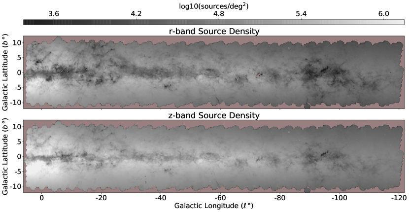
Figure 1: DECaPS2 source density map (using a HEALPix grid at NSide = 512) in $r$-band (top) and $z$-band (bottom) using a common, logarithmic color scale. This figure employs a cut requiring sources be brighter than 19th magnitude in the reported band and be detected in at least one of the two immediately adjacent bands.

Measuring the fluxes of stars in images of the Galactic plane is complicated by nebulosity, crowding, and numerous faint sources. We broadly refer to the presence of structured emission and absorption regions, such as filaments or clouds of gas and dust (H$II$1.2exregions, dark nebulae, reflection nebulae, etc.) as “nebulosity.” Most photometric pipelines model images as the sum of galaxies, point sources, and backgrounds that are smooth on scales much larger than the point spread function (PSF) (Stetson, 1987; Bertin & Arnouts, 1996; Lang et al., 2016; Schlafly et al., 2018). Thus, without explicit handling, nebulosity with fine spatial structure is often incorrectly modeled as the sum of many point sources or galaxies. Further, for real sources located near nebulosity, variations in flux associated with nebulosity can be incorrectly attributed to the source, biasing the estimated source flux (Saydjari & Finkbeiner, 2022).

Images of the Galactic plane also suffer from “crowding,” where light from different stars substantially overlap one another in images. At the single-exposure level, crowding complicates the identification of stars and the measurements of their fluxes. When sources have large angular separation, identifying stars via peaks in an image is easy (for large signal-to-noise ratios, or “SNR”) and source modeling is likewise straightforward. When two sources have zero angular separation, they should be modeled as a brighter single source with sum of the flux from both sources. The objective of modeling crowded fields of stars is to accurately measure the fluxes and positions of stars in between these two limits.

Crowding also complicates catalog construction. In many surveys, like DECaPS2, modeling is performed on individual exposures, and the resulting catalogs must be combined to form a multi-band, multi-epoch catalog. Variation in the estimated source locations and the overall number of estimated sources in different exposures complicates the notion of a single object list. One solution is to create a super object list from stacks of multi-epoch images and then perform forced-photometry at those object locations (Magnier et al., 2020). However, the creation of the super object list is hindered by the lack of a well defined PSF on the stacked images and by the astrometric precision of the stacking. Another solution is to identify and fit sources using all imaging touching a given location simultaneously (Dey et al., 2019). However, this prevents the massively parallel processing that can be used when individual exposures are processed independently. Progress has been made using transdimensional, probabilistic cataloging methods on single-exposures (Brewer et al., 2013; Portillo et al., 2017) or multi-band imaging (Feder et al., 2020; Liu et al., 2021), where the total number of sources in the image is not fixed. However, these methods are computationally expensive and have not yet been applied at scale (i.e., have only been applied to a tiny fraction of the sky).

As photometric surveys push deeper to observe fainter stars, a larger number of stars in the resulting catalog will be near the detection threshold. This is because the probability distribution of apparent stellar flux is approximately a power law, increasing in probability with decreasing stellar flux (Gorbikov et al., 2010). The detection threshold is often an explicit cut on the SNR of a peak relative to the background used during source identification (e.g. Schlafly et al., 2018). Even probabilistic methods have an implicit detection threshold set by the evidence required to predict a source with reasonable probability. However, only identifying sources above a threshold introduces a selection bias in sources with flux near the threshold. For example, for a source with true flux below threshold, only observations of the source where the realization of the noise deviates high will be identified, biasing the flux estimate high.

Another faint-limit bias arises from the common practice of using maximum-likelihood approaches to identify source locations (Portillo et al., 2020). The maximum-likelihood location prefers a source center capturing more of the flux in the image, even if that flux is noise, and thus biases flux estimates high. While both faint-limit biases described above can be partially mitigated by multi-epoch approaches, it is imperative to understand their form and realization in practice at the single-detection level to predict how these biases are modified by multi-epoch methods. Further, it is a pressing challenge to the community to correctly model these biases so that, when combined with the appropriate priors, better use can be made of the statistical power of the large number of faint sources in photometric surveys.

Synthetic injection tests are an important tool for evaluating the magnitude of bias introduced by nebulosity, crowding, and faint-limit selection effects. While the importance of synthetic injection tests has long been recognized, they have only recently been applied in large surveys. The Dark Energy Camera Legacy Survey (DECaLS, Dey et al. 2019) used Obiwan to inject synthetic galaxies into single-epoch images across multiple bands in a single patch (Kong et al., 2020). The Hyper-Suprime Cam Subaru Strategic Program (HSC-SSP) Survey (Aihara et al., 2018) used SynPipe to inject synthetic stars and galaxies into single-epoch images across multiple bands in two test tracts (Bosch et al., 2018; Huang et al., 2018). The Dark Energy Survey (DES, The Dark Energy Survey Collaboration 2005) used Balrog to inject synthetic galaxies into single-epoch images across multiple bands in a random 20% of exposures in the Year 3 release (Everett et al., 2022). In this work, we will describe how DECaPS2 uses crowdsource to inject synthetic stars into single-epoch images for a single band in a random 2% of exposures. While injecting into only a single band prevents analysis of single-object level color biases, this restriction allows crowdsource to perform injection tests at runtime and achieve, what is to our knowledge, the first full survey characterization of injection tests of synthetic stellar sources.

1.2 DECaPS2

We present the second data release of the Dark Energy Camera Plane Survey (DECaPS2), which provides optical and near-infrared photometry in the Galactic plane accessible in the Southern hemisphere with $\delta\leq-24\degree$. The combination of DECaPS2 with PS1 finalizes deep optical-NIR ($g\sim 24$th to $Y\sim 21$st mag) coverage of the entire Galactic plane. The source density in selected bands is shown in Figure 1. The DECaPS2 catalog contains 3.32 billion sources built from 34 billion detections using crowdsource (Schlafly, 2021), a photometric pipeline optimized to handle crowded-field photometry. A new synthetic injection module for crowdsource was used uniformly throughout the survey footprint to rigorously benchmark photometric performance and constrain uncertainties so as to enable interpretable downstream statistical inference.

We further develop, validate, and implement a new method to handle structured backgrounds (nebulosity) ubiquitous in the Galactic plane (Saydjari & Finkbeiner, 2022). To do this, we perform a statistical interpolation of nebulous structures to correct both the flux and flux uncertainties of stars. We use the injection tests to quantitatively characterize the photometry as a function of blending between two neighboring sources in order to better understand the intermediate separation regime. In the faint limit, we derive a convenient fitting form of the single-exposure threshold bias. Combined with the bias from using the maximum-likelihood position, we show that the faint-limit bias can be used as an empirical measure of the photometric depth. Applying corrections for these biases requires a more careful treatment of the combination of detections into objects than that performed in DECaPS2. However, we both introduce a model that captures the faint-limit behavior and demonstrate the utility of understanding these biases, which are important steps toward obtaining usable photometry near survey thresholds.

Table 1: Summary of DECaPS Imaging

Filter	Wavelength Range (nm)	Exposure Time (s)	Number of Exposures	On Sky Time (h)
g	398.0 - 548.5	96	4440 (3685)	118 (98)
r	565.5 - 717.0	30 [50]	4386 (3644)	39   (33)
i	704.5 - 858.0	30	4345 (3550)	36   (30)
z	846.5 - 1000.0	30	4343 (3526)	36   (29)
Y	950.0 - 1034.0	30	3916 (3292)	33   (27)

This work presents the second data release, which we refer to as DECaPS2. When referring to imaging, we use DECaPS2 to refer to those images taken after the first data release of DECaPS (Schlafly et al., 2018), which we refer to as DECaPS1 for both the imaging and catalog hereafter. When referring to the photometric catalog, DECaPS2 refers to a new reduction which processed both DECaPS1 and DECaPS2 imaging. The main differences compared to the first data release are increased sky coverage in Galactic latitude from $|b|<4\degree$ to $|b|\leq 10\degree$ and improvements in the photometric reduction.

The DECaPS2 catalog contains high-quality photometry with rich information about both the composition and structure of the dust and stellar populations in the Milky Way. Our work on nebulosity, crowding, and faint-limit biases may inform the next generation of photometric pipelines necessary to handle imaging of the Galactic plane planned for the Nancy Grace Roman Space Telescope (Akeson et al., 2019) and the Legacy Survey of Space and Time (LSST) at the Vera C. Rubin Observatory (Jones et al., 2020).

2 Observations

All observations associated with DECaPS were obtained using the Dark Energy Camera (DECam, Flaugher et al. 2015) mounted on the 4m Victor M. Blanco telescope at the Cerro Tololo Inter-American Observatory (CTIO). The 2.2° diameter field of view, 0.26$"$/pixel plate scale, and arcsecond seeing (Section 7) make these observations well-suited to surveying and resolving even the extremely crowded inner galaxy. The survey imaged the Galactic plane $|b|\leq 10\degree$, $6\degree>\ell>-124\degree$ (2700 deg², 6.5% of the sky) in five broad photometric bands, $grizY$. The efficiency of DECam enabled observations to keep up with the survey footprint as it crossed the meridian and thus achieved very low airmass, with a mean of 1.17 and standard deviation of 0.15.

One of the goals of DECaPS is to capture a large fraction of stars with possibly high extinction in the Galactic midplane, probing distances out to the Galactic center. The exposure times were initially set to target the main sequence turn-off for a 10 Gyr, solar metallicity population of stars at eight kiloparsecs, through dust extinction of $E(B-V)=1.5$ mag. These target depths are 24.5, 22.3, 21.2, 20.6, and 20.3 (AB) mag in $grizY$. We reduced the target of 24.5 mag in $g$ to 24.1 mag in order to better balance the exposure times among the dark- & bright-time bands, given a minimum exposure time of 30s in each image in order to avoid being dominated by overheads. This led to exposure times of 96s in $g$-band and 30s in $rizY$-bands, and means that we only reach out to 1.4 mag $E(B-V)$ in $g$ but reach past the main-sequence turn-off in all other bands. We achieved these depths for all bands except for $g$-band (see Section 7.2).

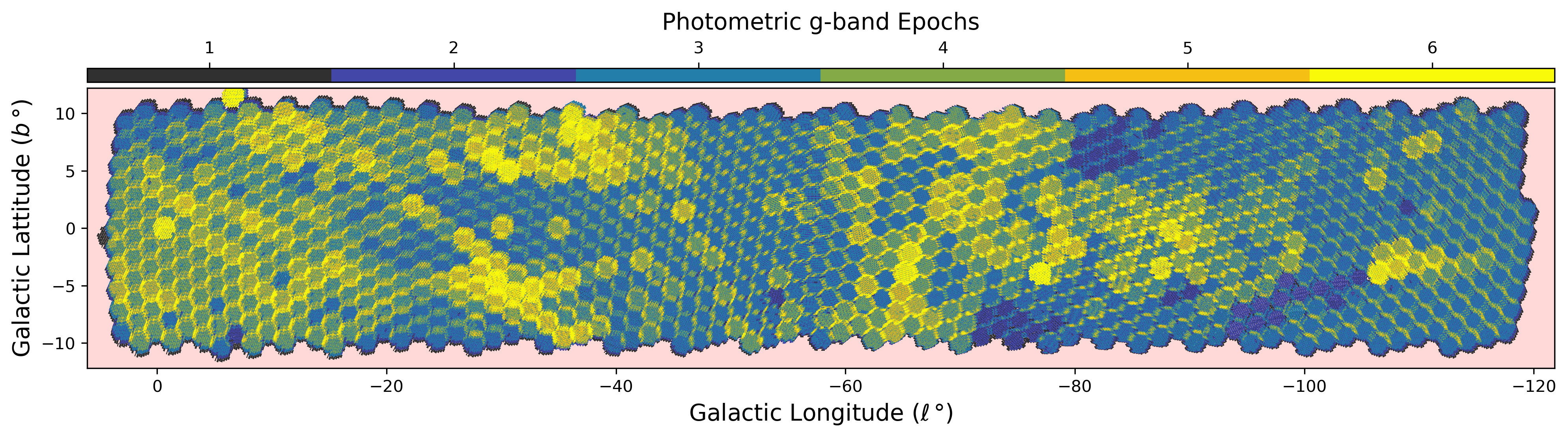
Figure 2: High resolution coverage map of the DECaSP2 survey footprint showing the number of photometric $g$-band visits. Small scale variations in coverage resulting from the tiling strategy and CCD failures are visible.

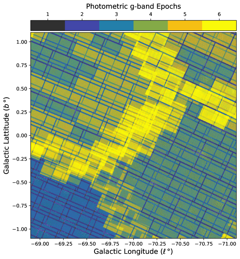
Figure 3: Zoomed-in version of Figure 2 at the scale of the focal plane of DECam.

The survey obtained a total of 21,430 exposures amounting to 260 hours of total exposure time over the duration of the program. DECaPS2 comprises observations starting in March 2016 and ending in May 2019. Approximately $83\%$ of exposures were of high enough quality to be included in our photometric catalog (see Section 3.2). A detailed per-band breakdown is provided in Table 1.

The survey strategy aimed for three overlapping visits (in every band) for the majority of the survey footprint, though the tiling pattern leads to some areas having a different number of visits. The tiling strategy used for DECaPS follows the strategy developed for the DECam Legacy Survey (Dey et al., 2019, DECaLS). The field centers of the three passes are offset relative to one another to fill in gaps in the DECam focal plane. The DECaLS tiling scheme had the unfortunate feature that DECam chip gaps partially overlapped in all three passes near right ascensions of 270°. We remedied this by adding an additional pass in this area with a small fixed offset relative to other passes in $({\rm RA}\cos({\rm DEC}),{\rm DEC})$ to cover the chip gap.

In addition, in regions with a low number of visits, there can be very small regions with no coverage following a spatial pattern matching CCD-level malfunctions on DECam. Further reductions in the coverage are attributable to some imaging not being suitable for inclusion in the photometric catalog, for example as a result of partial cloud cover (see Section 3.2). A representative high-resolution coverage map for the $g$-band data used to build the photometric catalog presented here is shown in Figure 2 and 3, and similar maps for the other bands are available in Section 9.

The three visits at a given location could occur the same night (rarely), on adjacent nights (more typical), or during observing runs a year apart. This mixing of temporal and spatial overlap of observations improves the ability of the calibration to constrain variations in throughput as a function of time, stabilizing the calibration over the long duration of the survey. We describe the major observing runs (a range of nights with more than 50 exposures each) in Table 2 and identify which filters were primarily used during that run. During each observing run, $0-6$ calibration exposures were taken of high latitude fields, which were usually 30s for $gr$-bands and 20s for $izY$-bands.

Observations include approximately 23 full nights, 29 half nights, and 12 quarter nights. We aimed to observe in the $gr$-bands when the Moon was down and $izY$-bands when the Moon was up. During run 7, $r$-band images were taken while the Moon was up and used 50-second exposure times to compensate for the brighter sky. As the survey progressed our planning software became more sophisticated, leading us to take better advantage of brief periods where the moon was down in a bright night, or vice versa, leading most runs to include observations in all of $grizY$. Runs 13 and 14 were impacted by a temporary mechanical failure of the filter wheel preventing observations in $Y$-band; run 15 skipped observations in $iz$ to focus on $Y$ to make up for the lost time.

Table 2: DECaPS Observing Runs

Run #	Date Range	Filters	# Nights	Notes
1	2016-03-13 to 03-16	$gr$	$4$	2016-03-16 clouded out
2	2016-03-23 to 03-26	$izY$	$4$	2016-03-25 clouded out
3	2016-08-10	$izY$	$0.5$	Scattered clouds
4	2016-08-14 to 08-16	$izY$	$2\times 0.5$	Scattered clouds
5	2016-08-22	$izY$	0.5
6	2016-08-23 to 08-26	$gr$	$4\times 0.5$	08-23 and 08-25 clouded out
7	2017-01-16 to 01-23	$r^{\star}izY$	$6\times 0.5$	01-22 and 01-23 clouded out ($r^{\star}$ used 50s exposure time)
8	2017-04-19 to 04-20	$grizY$	$2$	04-19 marginal
9	2017-04-27 to 04-30	$grizY$	$2+2\times 0.5$
10	2017-05-03 to 05-04	$grizY$	$2\times 0.5$	05-04 cloudy
11	2018-02-02 to 02-03	$izY$	$2\times 0.5$	02-02 marginal
12	2018-02-25 to 02-27	$grizY$	$3$	02-27 clouded out
13	2018-05-08 to 05-11	$griz$	$4\times 0.5$	05-08 clouded out
14	2018-05-18 to 05-20	$griz$	$3$	05-18, 05-19 marginal
15	2018-08-01 to 08-04	$grY$	$4\times 0.5$	08-02 clouded out, 08-04 marginal
16	2019-01-09 to 01-18	$grizY$	$10\times 0.25$	01-10, 01-13 marginal
17	2019-01-30 to 01-31	$grizY$	$2\times 0.25$
18	2019-04-25	$grizY$	$0.5$
19	2019-04-27 to 05-02	$grizY$	$5$	04-29 clouded out

3 Catalog Building

3.1 Single-Epoch Processing

Each exposure was processed in three serial steps by separate pipelines: the DECam Community Pipeline (CP), crowdsource, and CloudCovErr.jl.

3.1.1 DECam Community Pipeline

The DECam Community Pipeline (Valdes et al., 2014) is managed and run by NOIRLab and converts Raw exposures to the instrument-calibrated (InstCal) products that serve as inputs to user-managed photometric pipelines. In addition to images, these products include a per-pixel inverse variance (weight) map and an artifact mask. In this reduction, the CP performs the following steps (among others):

• overscan subtraction (bias correction)

• amplifier cross-talk correction

• static bad pixel masking

• saturation and bleed trail masking

• nonlinearity correction

• flat-field correction (dome and star flat)

• large reflection pattern (“pupil ghost”) removal

• large scale background gradient removal

• fringe correction

• astrometric WCS solution

• single exposure cosmic ray masking

For more details on the processing steps, see the NOIRLab Data Handbook. The CP excludes completely nonfunctional CCDs from its reduction which includes N30 for the full duration of the survey (damaged from an over-illumination event) and S30 from November 2013 to December 2016 (Runs 1-6, first half of DECaPS1). See Status of DECam CCDs from NOIRLab for more details. The CP has evolved over time, and we report the version numbers over time in Table 4.

Throughout the DECaPS2 observing period there were several changes in the header keywords, such as the reference catalog used for astrometric solutions and the CCD saturation levels. We observed cases where these changed without an accompanying change in the CP version number. The CP automatically and reliably provided calibrated images shortly following each DECaPS observing run. We note one minor flaw that had a significant impact on DECaPS2, however. In the majority of exposures (9377) taken during DECaPS2, the saturation thresholds were set slightly too high during the initial CP processing for seven CCDs (N3, N9, S13, S19, S20, S22, S26). The crowdsource pipeline uses the brightest 200 unsaturated stars for PSF fitting in order to limit the effects of blending, and elevated saturated limits can lead to substantial contamination of the PSF stars. This led to poor PSF fits on these CCDs and severely impacted our photometry. As such, we used the sensitivity of our PSF fits to help reset the saturation thresholds (see Appendix B) in the CP and reprocessed the impacted exposures (CP v5.5), resolving the issue.

Table 4: DECam Community Pipeline Versions

Version	# of Exposures	Date Range
v3.9.0	3780	2016-03-13 to 2016-03-27
v3.9.2	1845	2016-08-10 to 2016-08-27
v3.10.0	5	2016-03-24 to 2016-03-27
v3.12.0	1350	2017-01-17 to 2017-01-22
v4.1.0	5064	2017-01-25 to 2018-02-28
v5.2.3	12	2018-02-04 to 2018-02-04
v5.5	9377	2018-05-09 to 2019-05-03

Fringe correction is most important for Y-band where the longer wavelengths more easily form interference fringes across the CCD that need to be modeled and removed. However, we found that for 12 exposures the CP fringe-correction algorithm failed and visibly increased the amplitude of fringing on the InstCal images. The impacted exposures were reprocessed using no fringe correction (CP v 5.2.3). We note that DECaPS images pose more of a challenge than typical extragalactic fields to fringe fitting algorithms because of the large numbers of stars present in the images.

3.1.2 crowdsource

The photometric pipeline crowdsource takes in the InstCal products and estimates the PSF, finds the location of sources (deblending crowded fields), and estimates a variety of statistics about those detections, flux and flux uncertainty being among the most important. The crowdsource flux uncertainties simply combine the PSF estimates with the the InstCal inverse variance maps. Several improvements to crowdsource were made since DECaPS1, including a synthetic source injection module described in Section 7. Both a detailed description of the code and new features will be described elsewhere (Saydjari & Schlafly, 2022, in prep.).

Briefly, crowdsource applies an additional bad pixel mask and modifies the weight map so that CP-masked pixels (except bit 7) have zero weight (see Table 5). crowdsource also implements special handling for the partially functional CCD S7 where the gain of amplifier B is not stable. In several special cases, crowdsource reduces how aggressively it deblends. One case is around objects in a galaxy catalog, which is a new feature compared to DECaPS1. Another case is in regions identified as nebulous by a (band-agnostic) convolutional neural network (CNN), the “nebulosity CNN”, which was improved relative to DECaPS1. The algorithm proceeds by iteratively estimating the sky using a masked moving median, finding peaks in the PSF-convolved residual image, jointly estimating fluxes of all sources, and refining the PSF. In addition to the native crowdsource stopping conditions, we chose hard limits of a minimum of 4 and maximum of 10 iterations. The pipeline transitions between conservatively deblending sources and aggressively deblending sources on the third pass. A global maximum on the number of sources that can be found on a given CCD was set to $320,000$.

The PSF used was a model of the ideal-seeing instrumental response (static) from the Dark Energy Survey (DES, Abbott et al. 2021), which includes diffraction spikes and other features in the PSF wings, convolved with a 2D, possibly anisotropic Moffat (parametric). Additionally, per-pixel residuals were fit in the central $9\times 9$ pixels of the PSF to account for departures from a Moffat profile and added to form the final PSF model. The Moffat and core residual parameters were allowed to vary linearly across the CCD. The PSF model was refit at each iteration of source finding using up to the 200 brightest stars passing a quality cut (e.g., not saturated). Despite known variations in the PSF as a function of magnitude (i.e., the “brighter-fatter” effect, Stubbs & Tonry 2006; Antilogus et al. 2014), no such magnitude dependence was included here and the PSF model used is most representative of the bright stars used for the PSF parameter fitting.

The spatial extent of the PSF used to model a source depends on its flux, with larger extents used for larger fluxes. The intention in choosing the model extent is that the flux of a given star is captured down to a surface brightness significantly fainter than the per-pixel uncertainty in the sky. Roughly, the extents are $19\times 19$ pix for sources with peak per-pixel fluxes less than 1000 ADU, 59 pix for sources less than 20000 ADU, 149 pix for sources that are saturated or brighter than 20000 ADU, and 299 pix for sources within 5 pixels of a source in a “bright” star catalog—these saturate a large number of pixels, making flux estimates challenging.

A full description of the individual-image catalogs produced by crowdsource is available in Section 9. We describe three important quality-assurance quantities here since they will be discussed below. These quantities measure the overlap of a source with neighbors, the quality of the input data for the fit, and the quality of the fit.

The “blendedness” of an object is measured by fracflux, the PSF-weighted fraction of flux at the source location in the image that is coming from that source (as opposed to coming from surrounding sources). Pixels masked by the CP (zero weight in crowdsource) are excluded from the average. Very blended objects have fracflux of 0 while isolated objects have fracflux of 1. The precise definition is

$$\texttt{fracflux}=\frac{\int du\,N(u)\,P(u)\,\mathds{1}_{\left(\sigma^{-2}>0\right)}}{\int du\,I(u)\,P(u)\,\mathds{1}_{\left(\sigma^{-2}>0\right)}}$$ (1)

where the integral is over a region 5” $\times$ 5” (19 $\times$ 19 pixels) around the source (hereafter “stamp”), $P$ is the PSF (renormalized to sum to 1 on the “stamp”), and $\mathds{1}_{\left(\sigma^{-2}>0\right)}$ is an indicator function requiring that the inverse variance weights be nonzero (pixels not saturated, part of a cosmic ray, etc.). In the numerator, the integral is against $N$, which is the residual image plus the source model for the source of interest only (i.e., neighbor-subtracted image). In the denominator, the integral is against $I$, the image with all sources present.

The quality factor (QF) is the PSF-weighted fraction of good pixels (nonzero weight) within the stamp around the source.

$$\texttt{QF}=\int du\,P(u)\,\mathds{1}_{\left(\sigma^{-2}>0\right)}$$ (2)

Stars which coincide with a masked cosmic ray, occur near the edge of the detector, or are significantly saturated will have QF closer to $0.0$ while clean detections have a QF of $1.0$

The reduced chi-squared ($\chi_{r}^{2}$) is the PSF-weighted inverse variance-weighted squared residuals, normalized by the integral of the PSF-weighting of active pixels over the stamp (which is exactly the QF).

$$\chi_{r}^{2}=\frac{1}{\int du\,P(u)\,\mathds{1}_{\left(\sigma^{-2}>0\right)}}\int du\,\frac{R^{2}(u)}{\sigma^{2}(u)}\,P(u)\,\mathds{1}_{\left(\sigma^{-2}>0\right)},$$ (3)

where $R$ is the residual (image - model). Here the quality factor plays the role of the degrees of freedom by specifying the fraction of the effective area of the PSF that is used in the fit (has nonzero weight). The $\chi_{r}^{2}$ serves as a measure of goodness of fit of the PSF model to a given source.

3.1.3 CloudCovErr.jl

The source locations, PSF models, and residuals for each image are reprocessed by CloudCovErr.jl to correct the flux and flux uncertainties in the presence of structured (nebulous) backgrounds. CloudCovErr.jl works by predicting the distribution of possible backgrounds masked by the star. This interpolation (known as Local Pixelwise Infilling, LPI) actually predicts the distribution of residuals of those possible backgrounds relative to the smooth background model used by crowdsource, which reduces the fraction of the image that must be masked because of the presence of sources.

Table 5: crowdsource Bitmask

Bit	Description	Exclude Source?
		Catalog	Injections
0	No problems	No	No
1	Bad pixel	Yes	Yes
3	Saturated	Yes	Yes
4	Bleed Trail	Yes	Yes
5	Cosmic Ray	Yes	Yes
6	Low Weight	Yes	No
7	Difference Detection	No	Yes
8	Long Streak	Yes	No
20	Additional Bad Pixel	Yes	Yes
21	Nebulosity	No	No
22	CCD S7 amplifier B	Yes	No
23	Near Bright Star	No	Yes
24	Near Galaxy	No	Yes
30	No Deblend	No	No
31	Sharp	No	No

Note. — Bits $0-8$ are inherited from the CP, $20-24$ indicate a special region on the CCD or sky, and $30-31$ indicate a change in the crowdsource source identification parameters.

To do this interpolation, LPI trains a covariance matrix over the residuals of local data representative of the true background (unmasked). It then leverages pixels in an annulus around the star to obtain the conditional Gaussian distribution of the background residuals within the stellar footprint. The resulting flux uncertainty is quasi-independent of the InstCal inverse variance weights as it is estimated based on observed correlations of background pixels in the image nearby the source of interest. We refer to the background-corrected flux and flux uncertainty as cflux and dcflux, respectively.

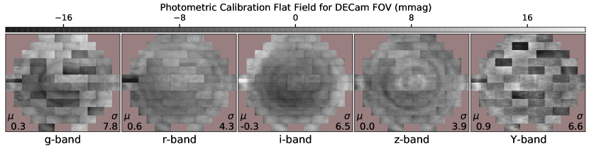
Figure 4: Time-invariant flat-field across the full DECam field of view produced during photometric calibration of DECaPS2. Each panel shows a different photometric band and the median and $\sigma_{\rm IQR}$ in mmag of the flat-field are in the bottom left and right corner, respectively. Gaps between CCDs of order 200 pixels are not shown in this large-scale representation. The sky orientation shown for the focal plane is north up, west right.

An additional output of CloudCovErr.jl is dnt, which is a quality flag on the correction algorithm. A table of possible nonzero values and the issues those bits indicate is available in Section 9. A detailed description of the method and validation of CloudCovErr.jl is provided by Saydjari & Finkbeiner (2022). Further, the precise parameter choices used with CloudCovErr.jl to process DECaPS2 are detailed in Section 5.1 of Saydjari & Finkbeiner (2022), so we do not repeat them here.

3.2 Photometric Calibration

The DECaPS2 photometric calibration follows the same procedure as DECaPS1 (Schlafly et al., 2019) which is based on the photometric calibration of SDSS (Padmanabhan et al., 2008) and PS1 (Schlafly et al., 2012; Magnier et al., 2013, 2020). Parametric models of the instrument and observing conditions are fit to minimize exposure-to-exposure variations in the measured flux of a given source. For DECaPS2, the model consists of a time-invariant flat-field correction, a system zeropoint per night, and a time-invariant term linear in the airmass (a constant “k-term” in the notation of Padmanabhan et al. 2008). From the calibration, we obtain a per-exposure zeropoint accounting for throughput variations between exposures to put all measurements on the same (relative) scale. Zeropoints were not allowed to vary at the CCD-level meaning that all CCD-level variations were assumed to be static and corrected by the time-invariant flat-field. We apply the following cuts to obtain high-quality sources used in the calibration:

• QF $>0.99$

• $-14<-2.5\log_{10}\left(\rm{\texttt{flux}}\right)<-12$ (instr. mags)

• $\chi^{2}_{r}/\left(1+\left(2\cdot 10^{-5}\times\texttt{flux}\right)^{2}\right)<2$

Each photometric band is fit independently.

Additionally, only exposures taken in ideal photometric conditions were included in the calibration. First, we manually inspected the photometric trends on each night and excluded observations taken in clearly non-photometric conditions. Then, as part of the determination of the photometric solution, we repeatedly solve for the calibration parameters using a linear least squares fit and apply them to all of the detections in the survey. At each iteration, we increasingly aggressively remove individual observations of stars discrepant with their mean magnitudes, as well entire exposures or CCDs when the measured fluxes are discrepant with the rest of the night or the rest of the exposure. For more details, see § 2.3 of Schlafly et al. (2012). A somewhat more relaxed photometricity cut is used for inclusion of a detection in the final calibrated flux of an object, defined below.

The flat-field correction treats each $256\times 256$ pixel² region of each detector independently and is shown in Figure 4. In Figure 4 and throughout the text we use $\sigma_{\rm IQR}={\rm IQR}/1.34896$ as a measure of scatter. The interquartile range (IQR) is an outlier robust measure of scatter, which should be $\sim 1.34896$ for the unit normal distribution. We then normalize the IQR by the normal value to provide an outlier robust measure of $\sigma$.

Offsets between adjacent CCDs are most apparent in $g$ and $Y$-bands. These offsets stem from slightly differing bandpasses for the different CCDs, and the different mean color used to construct flat fields in the CP and for the mean star in DECaPS. The edges and corners within a given CCD often differ slightly from the center of the chip, suggesting uncorrected throughput gradients across the CCDs that we are correcting. Amplifier B on S7, which has variable gain, sticks out clearly. Even with this low-resolution treatment, “tree ring” artifacts (concentric circles within a single CCD) from impurity migration during silicon growth are apparent, especially in the top right CCD (S29). Much of “tree ring” structure is at scales smaller than the $256\times 256$ blocking used in the flat-field and remains uncorrected.

There is a large radial gradient in $i$-band, attributed to a strong angle dependence of the $i$-filter bandpass. Radial rings are evident in most bands, especially $z$-band and are attributed to imperfect pupil ghost removal impacting initial CP flat-fields. In most cases, the photometric calibration accounts for small residuals from large corrections made by the CP. The small scatter ($<8$ mmag) in the flat-field per band is indicative of the accuracy of the CP, especially given that most of the signal in the worst bands ($giY$) stems from color-dependent effects for which any gray corrections like those attempted here are in some way unsatisfactory.

The stability of the photometric calibration is assessed using the residuals ($r_{\star}$) between the calibrated measured fluxes per detection and the average flux over all detections for a given calibration source. In Table 6, we report the average scatter of $r_{\star}$ per exposure as $\sigma_{\rm{cal}\star}$. The average $r_{\star}$ per exposure can be thought of as what the calibration would predict if the system zeropoint were allowed to vary per-exposure, even though the calibration fixes a global zeropoint per-night. The scatter of these “per-exposure zeropoints” ($\sigma_{\rm{ZP}}$) is a measure of the goodness of fit of the fairly static photometric model used (see Table 6). It describes at some level how close Cerro Tololo, the Blanco, and DECam approach the ideal of delivering perfectly repeatable fluxes night-to-night, adjusting only for an airmass and nightly throughput term; we find that it reaches this ideal at the 1% level. We clipped samples of the residuals per exposure to within $\pm 2.7\sigma_{\rm IQR}$ of the median before taking the mean and standard deviation in computing $\sigma_{\rm{cal}\star}$ and $\sigma_{\rm{ZP}}$, respectively.

Table 6: Photometric Parameters

Filter	$\sigma_{\rm{cal}\star}$ (mmag)	$\sigma_{\rm{ZP}}$ (mmag)	FWHM (”)	Depth (AB mag)
g	8.5	9.5	1.35	23.5
r	7.6	9.0	1.25	22.6
i	7.1	9.0	1.15	22.1
z	7.4	10.6	1.10	21.6
Y	7.0	9.0	1.07	20.8

We apply a cut on the per exposure scatter $\sigma_{\rm{cal}\star}\leq 20$ mmag and average zeropoint offset $\langle r_{\star}\rangle<200$ mmag to define “photometric” exposures ($\sim 83\%$ of the observations) that are included in the final DECaPS2 catalog. Additionally, individual CCDs are marked as excluded from the final fluxes when showing mean offsets ($\langle r_{\star}\rangle$) from the rest of the exposure more than $5\sigma$ larger than the typical offset in that band.

After applying this cut, we compute the same sigma-clipped statistics over all “photometric” exposures in Table 6. The $\sigma_{\rm{cal}\star}$ ranges from 7.0 mmag in $Y$-band to 8.5 mmag in $g$-band, and $\sigma_{\rm{ZP}}$ ranges from 9.0 mmag in $riY$-bands to 10.6 mmag in $z$-band. Under both of these measures, the photometric calibration is good to the $\sim 10$ mmag level, or around the $1\%$ level. Given that we neglect a careful treatment of the tree-ring distortions and better modeling of the DECam PSF, which lead to errors on the order of a few mmag, this is an excellent photometric calibration.

All of the above provides a relative calibration for variations in the atmosphere plus instrument throughput exposure-to-exposure, but does nothing to set the absolute zeropoint of the survey. For DECaPS2, we tie the absolute zeropoint to PS1, which in turn ties its zeropoint to HST; see Section 6.2. Various revisions of PS1 processing have altered the absolute zeropoints per band by $11-33$ mmag. Thus the relative calibration of DECaPS2 is at a precision comparable to the accuracy of the absolute zeropoint.

3.3 Constructing Objects

After calibration, detections from single exposures across all photometric bands are merged into objects using the Large Survey Database (see Section 9). Briefly, for each exposure, a k-d tree is constructed per detection to find the nearest neighbor in the list of previously known objects. If the nearest neighbor object is closer than a threshold radius (0.5”), that detection is assigned to that object. If the nearest neighbor object is further than the threshold radius, a new object is created for that detection. By this method, each detection is associated with one and only one object. Note that objects can be closer than 0.5” if they are created from detections in the same exposure where neither object had previously been found. Exposures are processed in temporal order.

Once detections are associated with objects, average properties of each object are computed. Per object, the position is determined by a simple mean (over all photometric bands) and the position uncertainty is the standard deviation of the detection positions. The mean MJD, maximum - minimum MJD, and total number of detections (over all photometric bands) of the object are also reported.

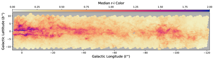
Figure 5: Median $r-i$ color for sources in the DECaPS2 catalog across the survey footprint (NSide = 512). This figure employs a cut requiring sources to be brighter than 19th magnitude in the $i$-band and be detected in $r$-band.

In each band, we report the number of detections and the average flux, computed as a weighted mean. The weights used throughout are the inverse of the reported flux variance from the photometric pipeline, with a term added in quadrature to account for multiplicative errors in flux estimation (for example, errors due to PSF mismodeling) on the order of 0.01 mag.

$$\rm{\texttt{weight}}=\frac{1}{\rm{\texttt{dflux}}^{2}+\left(0.00921\times\rm{\texttt{flux}}\right)^{2}}$$ (4)

We report both the (weighted) standard deviation of the detection fluxes from this mean and the uncertainty associated with the mean weight. Even though there are only three visits on average, the 25th-percentile, median, and 75th-percentile flux are reported. These flux-related statistics are computed for both flux and cflux.

A rough magnitude limit, which corresponds to $-2.5\log(5\times\rm{\texttt{dflux})+{\rm zp}}$, where ${\rm zp}$ is the exposure zeropoint, is reported per object as a maximum over all detections. This magnitude limit is an approximate estimate of the photometric depth at which that source would be only a $5\sigma$ detection. We discuss the spatial dependence of the magnitude limit of DECaPS2 further in Section 7.2.

Positional, epoch, and number of detection-related quantities are reported both over all detections and over only OK detections, which are deemed to be of high-quality. Flux-related quantities (and flags) are only computed for OK detections. Detections are OK if no bad flag bits were set for the center pixel (see Table 5), the flux uncertainty is nonzero, and the QF and $\chi^{2}_{r}$ pass the cuts outlined in Section 5.

All flux-like quantities are reported in units of “maggies” (Mgy), which are equivalent to 3631 Jy and are a convenient unit such that $-2.5\log_{10}(\texttt{flux})$ is in AB magnitudes. Throughout the band-merged catalogs, fields that cannot be populated are replaced with zero. For example, this occurs when there are no detections in a one of the bands for an object. Thus, it is imperative that a $\texttt{nmag}>0$ or $\texttt{nmag\_ok}>0$ cut is applied before using the per-band fluxes. Here nmag and nmag_ok are the number of detections (or OK detections) for a given object per band (see Section 9 for more).

The crowdsource quality metrics fracflux, QF, and $\chi_{r}^{2}$ as well as the CloudCovErr.jl quality metric cchi2 are reported as a (weighted) average per-band. The (weighted) average flux/dflux and predicted class probability from the nebulosity CNN are also reported. The dnt bitmask for CloudCovErr.jl and the flag bitmask for both crowdsource and the CP were propagated with both a bitwise AND and OR to show if a given bit was thrown for all or any of the detections, respectively.

A complete description of all fields in the band-merged catalogs is available in Section 9.

4 Catalog Characterization

Using the crowded-field photometry code crowdsource, we created a catalog of 3.32 billion sources from 34 billion detections in the DECaPS imaging. We further post-processed those photometric outputs using CloudCovErr.jl to improve the flux and flux uncertainty estimates in the presence of structured backgrounds (such as clouds of gas and dust). We present the catalog here and its validation in the next section.

We visualize the source density in r- and z-band in Figure 1 (using a HEALPix grid at NSide = 512 resolution, Górski et al. 2005). In both, reductions in source density are apparent as a result of dust clouds. However, the relative reduction is less pronounced in z-band, illustrating that our NIR photometry penetrates to greater distances through dusty regions. Source densities over the survey footprint for the other photometric bands are available in Section 9.

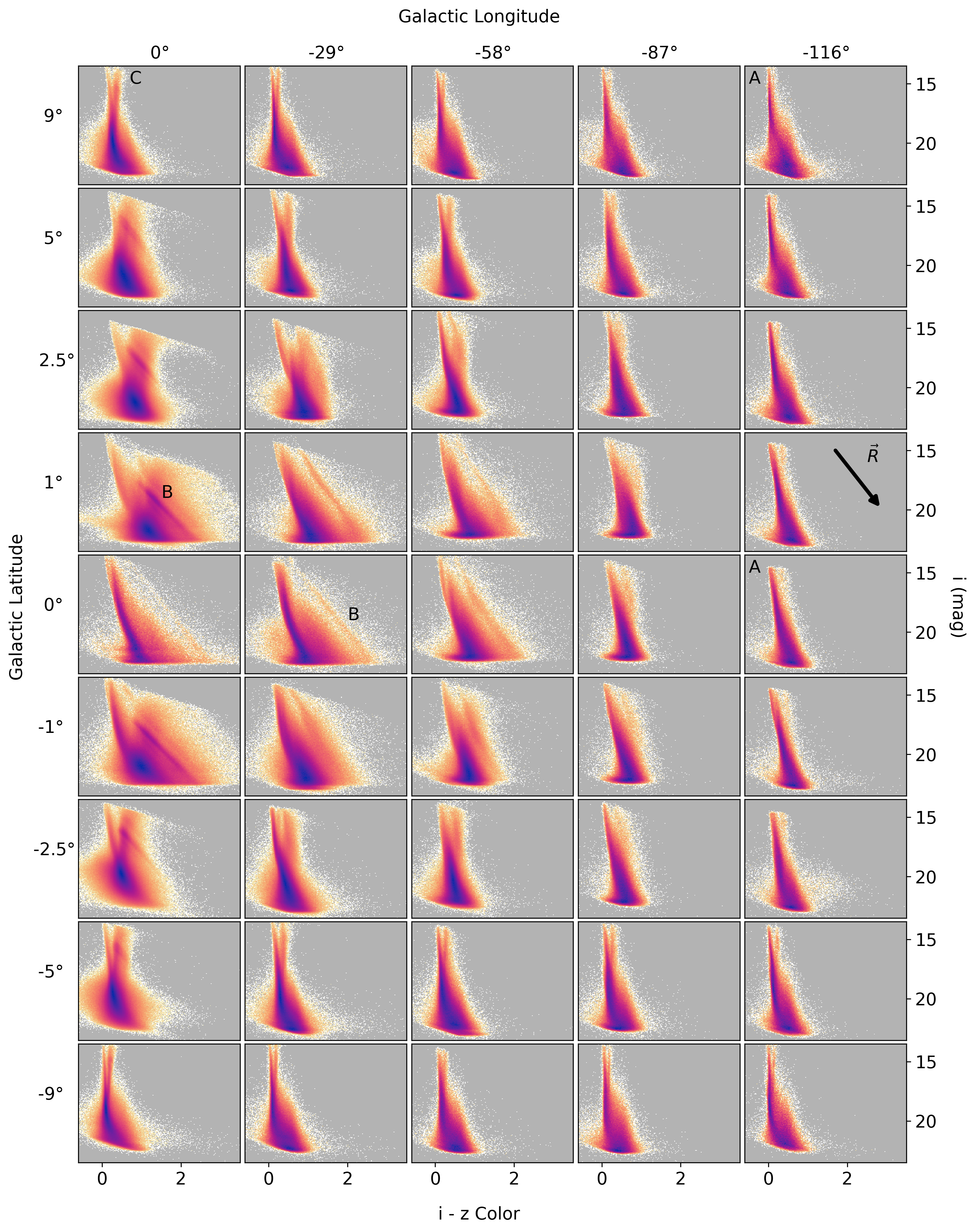
Figure 6: Color-magnitude diagrams (CMDs) in $i$ versus $i-z$ for a beam of radius $0.5\degree$ on a grid of Galactic latitude and longitude over the survey footprint. Each CMD color scale is in log-density and has its own normalization (light, white, low; dark, blue, high density). The features associated with blue main sequence stars in the disk (A), red clump stars (B), and red-giant-branch stars (C) are labeled. Reddening vector showing effect of dust plotted in ($-116\degree$, $1\degree$) for reference.

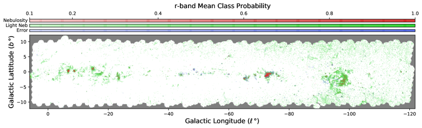
Figure 7: Classification of the DECaPS2 $r$-band imaging by crowdsource nebulosity CNN. Three of the four possible classes are shown as increasing opacity RGB color (nebulosity, light neb, and error) and the fourth class (normal) can be inferred by taking the complement. Each NSide = 512 HEALPix pixel displays the mean probability of each class over all photometric detections in the region. The probability associated with each source detection is the class probability of the pixel closest to the center of the source.

Globular clusters (down to 9th V-band mag) are already visibly prominent in the source density map as high density points in Figure 1. The homogeneous stellar populations provided by these globular and open clusters along relatively dusty lines of sight can help better constrain the stellar modeling uncertainties associated with reddening models. Of the 157 globular clusters in the 2010 edition of the Harris catalog (Harris, 1996), 47 fall in the DECaPS2 footprint (34 in DECaPS1). Of the 2858 open clusters in the Milky Way Star Clusters Catalog (Scholz et al., 2015), 972 fall in the DECaPS2 footprint (783 in DECaPS1).

In a few cases, high-density points are the result of spurious sources fit to massive pupil ghosts near very bright stars. Notable examples are $\gamma$ Crucis ($300.2\degree$, $5.6\degree$, V = 1.6 mag), $\lambda$ Velorum ($265.9\degree$, $2.8\degree$, V = 2.2 mag), and $\eta$ Canis Majoris ($242.6\degree$, $-6.5\degree$, V = 2.5 mag). We use these in part to develop the quality cuts designed to remove spurious sources (see Section 5).

4.1 Dust Diversity

In the Galactic midplane, variations in the median $r-i$ color of stars (Figure 5) are dominated by reddening of the starlight from dust, and thus acts as a tracer for dust density. However, for regions with very dense dust clouds, the median star lies in front of the cloud, and thus a line of sight will only appear to have less reddening (since there are no sources found behind the dust cloud). A transition to this case occurs around $|b|=\pm 1$ toward the Galactic center.

The DECaPS2 survey footprint includes famous dust clouds such as Pipe, Lupus, Circinus, the Coalsack, the Vela Molecular Ridge, and portions of Musca and Ophiuchus, all of which appear prominently in the median $r-i$ color map (Figure 5). The high-quality photometry from DECaPS2 through a large range of extinction and across a diversity of structures will prove useful in probing the variation of dust properties throughout the disk, as was demonstrated already in the PS1 footprint (Schlafly et al., 2016, 2017).

4.2 Stellar Diversity

To illustrate the variety of stellar populations captured by DECaPS2, we show (apparent) color-magnitude diagrams (CMDs) in $i$ versus $i-z$ for $0.5\degree$ radius beams in a grid across the survey footprint (Figure 6). Each CMD has its own log-density normalization. These sight lines sample a large range of extinction and stellar densities and capture the transition from the Galactic bulge to the Galactic disk.

We expect detailed stellar investigations to be developed as follow-up work to this data release and point out only a few major features (and their variations) that are readily apparent. At high latitudes, ($-116\degree$, $9\degree$), we observe a sharp vertical track (A) from blue main-sequence stars in the Galactic disk. That track widens and tilts in the direction of the reddening vector (indicated by $\vec{R}$ in Figure 6) as the latitude approaches the plane and experiences more extinction from dust ($-116\degree$, $0\degree$). Moving toward that Galactic center ($0\degree$, $0\degree$), a parallel track along the reddening vector is observed (B) associated with red clump stars.

The long red clump track (B) observed in ($0\degree$, $1\degree$), resulting from variations in reddening from dust, tightens to more closely resemble the expected clump at higher latitudes where there is less differential extinction ($0\degree$, $2.5\degree$) before disappearing at the highest latitudes above the Galactic bulge ($0\degree$, $9\degree$). Variable ceilings in the maximum stellar magnitude, coming from a cut removing saturated sources in $z$-band, are apparent in several fields, including ($0\degree$, $2.5\degree$).

We also observe a track (C) with positive slope that is redder than A which we attribute to the red-giant branch (with contributions from either the disk, bulge, or both). Along certain lines of sight, such as ($-29\degree$, $-2.5\degree$) and ($-58\degree$, $2.5\degree$), there are tracks between A and C and ($-58\degree$, $2.5\degree$) which are likely associated globular/open clusters. In $g-r$ (see Section 9) a track bluer than A is observed along two lines of sight. The apparent gap in the main sequence, observed along several high latitude lines of sight, ($-116\degree$, $9\degree$) for example, could be a signature of probing different components (thin and thick) of the disk. We believe the high-quality photometry delivered by DECaPS2 over these diverse fields should provide a wealth of information that aids in solving the coupled problems of stellar evolution, Galactic structure, and dust density and reddening variations.

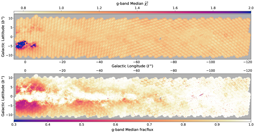
Figure 8: Median $g$-band $\chi^{2}_{r}$ (top) and fracflux (bottom) over all objects in the survey footprint.

4.3 Nebulosity

As discussed in Section 3.1.2, crowdsource uses a CNN to identify regions of nebulosity and reduces the degree of targeted deblending in those regions to avoid attributing diffuse emission to the sum of many small point sources. To do so, the CNN reports a probability that a given image sub-region (512 $\times$ 512 pixels) is in one of four classes:

• nebulosity, containing significant contamination by nebulosity

• light neb, containing faint nebulosity

• normal, no contamination

• error, containing artifacts from bright star pupil ghosts or spurious sky-level fluctuations introduced by the CP

These classes were trained on human-sorted representative images and are, in part, subjective. To elucidate what features each class actually corresponds to, we show the response of the CNN to $r$-band images across the survey footprint (Figure 7). The map encodes the class probabilities as the transparency of RGB channels for nebulosity, light neb, and error classes, respectively. The normal class probability is the complement of the sum of the other three.

The nebulosity class appears to dominate along ridges or cores surrounded by regions where light neb dominates. This nested behavior validates light neb and nebulosity as characterizing different degrees of the same physical feature. The features with large nebulosity or light neb probability strongly resemble the main features in H$\alpha$ maps, tracing emission nebulae in the Gum catalog, for example. Notable nebulae visible in the probability map include Lobster ($353.2\degree$, $0.9\degree$, NGC 6357), Cat’s Paw ($351.1\degree$, $0.5\degree$, NGC 6334), Prawn ($344.8\degree$, $1.6\degree$, IC 4628), and Carina ($287.6\degree$, $-0.6\degree$, NGC 3372). In addition, a large shell associated with the Vela supernova remnant is seen. Since H$\alpha$ emission is the primary source of nebulosity in $r$-band, this correlation validates the accuracy of the CNN in identifying the features of interest in practice.

The error class has high probability in a few points scattered across the footprint. These correspond to several extremely bright stars such as, $\lambda$ Velorum ($265.9\degree$, $2.8\degree$, V = 2.2 mag), $\alpha$ Crucis ($300.1\degree$, $-0.4\degree$, H = 1.3 mag), and $\beta$ Crucis ($302.5\degree$, $3.2\degree$, V = 1.3 mag). This validates the response of the error class to artifacts, such as those from pupil ghosts of bright stars. Further the error class probability is elevated around bright nebula, such as Carina, where spurious sky-level fluctuations are most common.

Table 7: Quality Cut Counts (in Millions)

Cuts	Any(grizY)	g	r	i	z	Y	All(gr)	All(izY)
Detections	34,032	4,939	6,783	7,538	8,417	6,355	-	-
+flags	33,476	4,850	6,674	7,414	8,277	6,262	-	-
+flags+QF	33,216	4,808	6,622	7,357	8,211	6,218	-	-
+flags+$\hat{\chi}^{2}_{r}$	33,138	4,792	6,616	7,334	8,178	6,218	-	-
+flags+QF+$\hat{\chi}^{2}_{r}$	32,896	4,754	6,567	7,282	8,117	6,177	-	-
Objects	3,319	1,405	1,911	2,330	2,588	2,092	1,288	1,804
+fracflux	1,558	784	1,000	1,203	1,285	1,090	722	929

Note. — Detection counts (for all bands and per band) and how they are modified by cuts on crowdsource quality metrics. These detection level cuts are used to define OK detections at the object level. Similar counts for objects before and after applying a cut at fracflux of 0.75. Counts for objects with detections in both $g$ and $r$-band and all three of $i$, $z$, and, $Y$-band shown in last two columns.

The final nebulosity mask used to change the deblending in crowdsource affects an even smaller area than those highlighted in Figure 7. These regions are indicated by sources with bit 21 set and per-CCD mask images saved in the single-exposure catalog files (see Section 9). The decision boundary for the nebulosity mask is

$$\frac{p(\texttt{nebulosity})+0.5\,p(\texttt{light neb}))}{p(\texttt{light neb})+p(\texttt{normal})+p(\texttt{error})}>2$$ (5)

This boundary was selected conservatively, to mask only the most nebulous regions in order to apply the full deblending power of crowdsource to the vast majority of the survey footprint. However, irrespective of any boundary selection, it is clear from Figure 7 that most of the sky is seen to be normal by the CNN, as desired.

4.4 Fit Quality

We use $\chi^{2}_{r}$ and fracflux for all objects over the survey footprint as indicators of variations in the quality of fit. When analyzing $\chi^{2}_{r}$ throughout this work, we rescale $\chi^{2}_{r}$ to give $\hat{\chi}^{2}_{r}$, using the flux of the source to prevent multiplicative systematics from dominating in the bright limit.

$$\hat{\chi}^{2}_{r}=\frac{\chi^{2}_{r}}{1+\left(10^{-5.5}\times\texttt{flux}\right)^{2}}$$ (6)

The choice of constant in Equation 6 is described in Appendix B and becomes important for sources brighter than $-13.75$ instrumental mags ($\sim 16.2$ g-band mag).

The median $g$-band $\hat{\chi}^{2}_{r}$ is $\sim 1$ for most of the survey footprint, indicating an excellent goodness of fit in most cases. The $\hat{\chi}^{2}_{r}$ is elevated in the most crowded regions, specifically the southern Galactic bulge, where PSF estimation can be difficult in the presence of such extreme blending.

In addition to variations resulting from Galactic structure, there is residual hexagonal pattern noise, especially near the higher latitudes taken later in the observing program. Specifically, the $\hat{\chi}^{2}_{r}$ increases toward the edge of the focal plane. We attribute this pattern to variability in the quality of PSF estimation for the different CCDs in the focal plane. In addition to PSF variations as a function of position in the field of view (see Appendix A), each of the DECam detectors has a slightly different nonlinear onset and saturation level, which can vary over time. As discussed in Appendix B, the impact of underestimated saturation levels on the $\hat{\chi}^{2}_{r}$ was so severe that we reprocessed most of the DECaPS2 observations, which significantly reduced the amplitude of the hexagonal pattern noise seen here. Some of the discrete steps in $\hat{\chi}^{2}_{r}$ may be explained by version changes in the CP, including an improvement in weight estimation between version 3 and 4—that is, the steps may reflect changes in the CP uncertainty rather than actual differences in the match of the model to the data.

The median $g$-band fracflux over the survey footprint appears to predominantly track source density. In regions of high source density, such as the southern Galactic bulge, the median fracflux is $\sim 0.5$. At higher latitudes, or in the presence of strong foreground dust extinction preventing the detection of most stars, we see the median fracflux approaches $\sim 1.0$, as it should for isolated sources. Small fluctuations of order $\sim 0.05$ tracking the hexagonal tiling pattern can be seen in some regions of the footprint, most notably at ($-75\degree$, $10\degree$) and ($-35\degree$, $-10\degree$).

Specifically, the median fracflux decreases toward the edge of the focal plane. This appears related to variations in the PSF FWHM in pixels over the field of view shown in Appendix A, though we have not identified the exact connection. The regions where this pattern is most notable are regions with unusually poor seeing or highly variable seeing between different visits. However, the overall smooth variation of fracflux throughout the survey footprint is a testament to the photometric uniformity of the survey, measured here through the deblending stability.

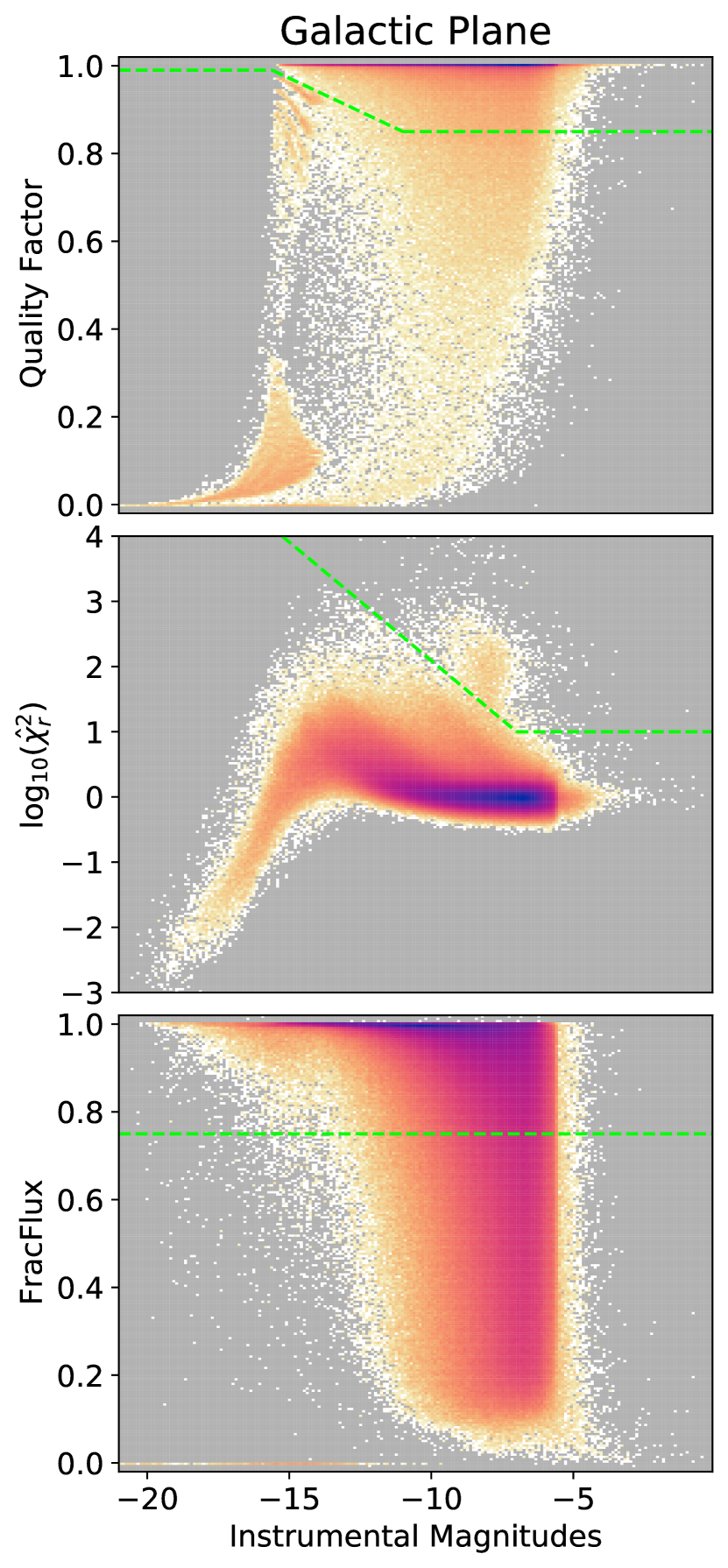
Figure 9: Distribution (2D histogram) of source detection as a function of instrumental magnitude and QF (top), $\log_{10}\hat{\chi}^{2}_{r}$ (middle), fracflux (bottom). Detections shown are in $r$-band for a typical line of sight ($0.5\degree$ radius) toward the Galactic plane ($\ell$,$b$) = ($-65\degree$, $0\degree$), with no cut on photometricity. Edge case sources with negative flux are excluded. The color scale is in log-density and each panel has its own normalization (light, white, low; dark, blue, high density). Quality cuts are shown as green-dashed lines.

5 Suggested Quality Cuts

We discuss different populations of photometric outputs as they appear under metrics of the photometric fit at the detection level. We then describe the detection-level cuts we apply to define OK detections that are used in constructing the object-level catalog. We conclude by evaluating the distribution of objects in terms of the bands in which they are detected and how an object-level cut impacts that distribution.

At the per-band object level, we describe a cut requiring:

• nmag_ok $>0$ (mandatory)

• fracflux $>0.75$ (optional)

The first cut is mandatory as a result of the catalog construction (see Section 3) and the second provides a possible cut to yield an extremely conservative “high-quality” catalog.

Further cuts at the object level on

• the average $\hat{\chi}^{2}_{r}$,

• the total number of OK detections, or

• requiring OK detections in multiple bands

could be explored for various applications.

In Figure 9, we show the distribution of $r$-band detections for a typical line of sight ($0.5\degree$ radius) toward the Galactic plane ($\ell$,$b$) = ($-65\degree$, $0\degree$), where no cut on photometricity is applied. Rare sources with negative flux are excluded. In the top panel, the distribution is QF as a function of instrumental magnitude. At the far left, ridges $\texttt{QF}\sim 0.7-0.95$ and a large foot $\texttt{QF}\sim 0-0.3$ are associated with sources at or near saturation. The highest ridge remains even after a cut on CP flags. For moderately faint sources ($-12$ to $-6$ inst. mag), most sources have QF $\sim 1$, but a broad distribution all the way to $0$ is observed. Sources in this distribution with lower quality factor tend to be closer to the chip edge or are more likely to be spurious detections associated with artifacts (bleed trails, cosmic rays). There is no sharp transition between “good” and spurious detections in this broad distribution, so we cut at $0.85$ to be consistent with DECaPS1. The final detection-level cut on QF (green-dashed boundary) linearly connects the faint $0.85$ cut and a cut at $0.99$ to eliminate sources exhibiting characteristics of saturation.

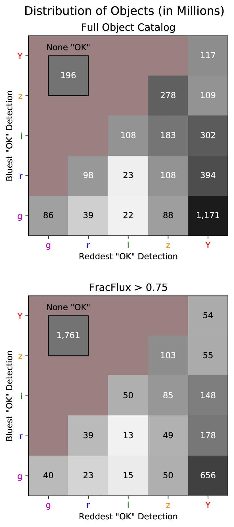
Figure 10: DECaPS2 objects grouped by the bluest and reddest bands in which that object has an OK detection. The number of objects (in millions) is shown and each entry is colored based on its relative proportion of the sample (logarithmic color scale, white low, black high). Sources with no OK detections are shown as an inset. The top panel uses the usual definition of OK detection while the bottom panel additionally requires fracflux$>0.75$.

The middle panel shows $\log_{10}\hat{\chi}^{2}_{r}$ as a function of instrumental magnitude. For moderately faint sources ($-12$ to $-6$ inst. mag), the $\hat{\chi}^{2}_{r}$ is centered at 1, indicating a good fit. The center of the $\hat{\chi}^{2}_{r}$ distribution increases to $\sim 10$ before turning over and rapidly decreasing toward $0$. The exact values here are strongly dependent on the regularization applied to convert $\chi^{2}_{r}$ to $\hat{\chi}^{2}_{r}$, but the sources after turnover are all saturated and removed by cuts on CP flags. There are two main populations of larger $\hat{\chi}^{2}_{r}$ sources at the faint end. An approximately vertical track around $-7$ with $\hat{\chi}^{2}_{r}\sim 100-1000$ is primarily associated with spurious sources around artifacts, particularly unmasked cosmic rays, which sometimes escape the CP cosmic ray finder especially in crowded fields. Sources in a diagonal track increasing in $\hat{\chi}^{2}_{r}$ with increasingly source flux are more likely to be: (1) one or more sources used to approximate a galaxy or (2) either real or spurious sources in the wings of bright sources. In these cases, it is more difficult to distinguish spurious from real populations. Thus, we suggest a detection-level $\hat{\chi}^{2}_{r}$ cut that only eliminates the first subpopulation (green-dashed boundary).

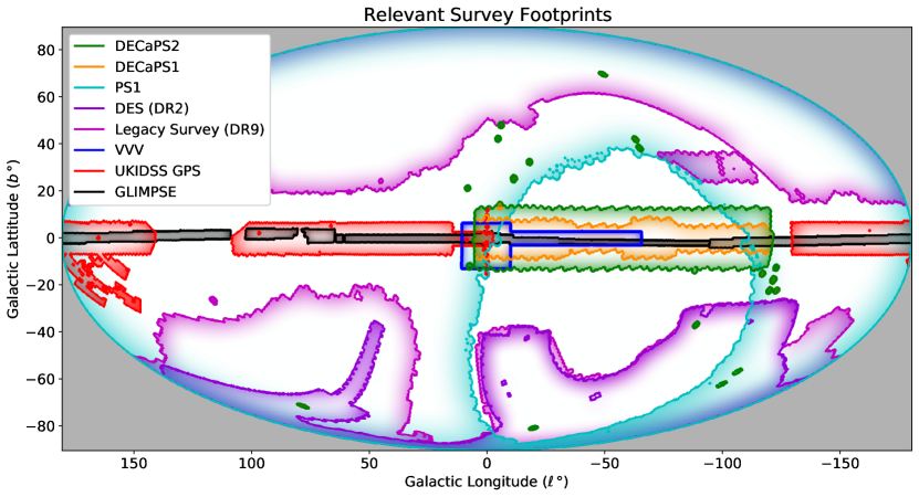
Figure 11: Mollweide projection in Galactic coordinates of large survey footprints with spatial or photometric coverage overlapping DECaPS2. The boundaries of each footprint are shown with shading on the side the survey covers. Gaia, 2MASS, and WISE are not shown because they are all sky surveys.

The bottom panel shows fracflux as a function of instrumental magnitude. For faint sources ($-12$ inst. mag and fainter), the fracflux distribution peaks at $1$, but has a broad distribution extending to $\sim 0.1$. Presumably, below $\sim 0.1$ the faint source is simply not deblended from the nearby brighter source(s). In Section 7.4 we find a minimum fracflux of 0.3 for SNR $9-10$ sources. There is a second mode to the fracflux distribution for bright sources ($<-15$) and a population of bright, fracflux 0 sources. Both are eliminated by CP flags and relate to saturation effects. While we do not impose a quality cut at the detection level for fracflux, we find evidence in Section 7.4 via injection tests that fracflux $=0.75$ provides a conservative cut to eliminate sources for which deblending the source and its neighbor into one or two sources is uncertain. Since this cut is independent of magnitude, it can be applied on the object catalog as desired in a given analysis using the DECaPS2 products.

Because the error modes caught by cuts on QF and $\hat{\chi}^{2}_{r}$ are best represented in instrumental magnitudes, we apply these cuts prior to merging detections into objects. We confirmed the generality of these cuts across all five filters and for several pointings with different stellar densities. The equivalent distributions for Figure 9 at the object level have all CP flagged populations (i.e., saturated sources) and sources within the detection level cuts above removed. At the object level, magnitudes are calibrated and on the AB system; thus there is slight broadening of the object distributions due to variable zeropoints between exposures. Table 7 provides the number of detections and objects before and after these cuts. Tighter cuts imposed on $\log_{10}(\hat{\chi}^{2}_{r})$ or a cut on the probability that the region of the image around the source was of class error could provide even more conservative catalogs.

It is also important to apply these cuts in defining OK detections at the detection level because of failure modes in detection-object association in the catalog construction. Detections are either correctly assigned to an object or are subject to object-object, object-spurious, spurious-spurious confusion. In the first confusion case, the detection belongs to a real object (which may not exist in the catalog), but is assigned to another real object. In the second, a spurious detection (from a cosmic ray or diffraction spike residual) is incorrectly assigned to a real object. In the last case, a spurious detection is assigned to an object which was created off of another spurious detection. Since every detection is associated with an object and there are limits for the separation between objects after the first exposure ingested into the catalog, we know all of these failure modes likely occur, though to different extents.

In Figure 10 we group objects by the bluest and reddest band for which that object has a detection which is OK (see Section 3.3). The diagonal of Figure 10 (top) represents the number of objects with OK detections in only one band. To the right of the diagonal, objects have OK detections spanning a larger range of photometric bands. The object counts in Figure 10 do not check that all intervening bands, between the bluest and reddest OK bands, have OK detections. However, our expectation for real objects is that they should be observed through a contiguous range of photometric bands. To ensure that the sum of object counts in Figure 10 is the total number of objects in the catalog, we also included a count of objects which have no OK detections. Given that OK detections require no bad flags from the CP at the central pixel of the source (see Table 5), saturated sources are an example of a real source expected to have no OK detections under this definition.

In the bottom panel of Figure 10, the same grouping of the DECaPS2 objects are shown with the additional constraint that fracflux$>0.75$ for a detection to be OK. Multi-band detections in $gri$-bands are less impacted by the fracflux cut as compared to $zY$-bands. This cut decreases the number of objects with OK detections in a single band by a factor of $\sim 2$. This reduction agrees with the intuition that faint spurious sources associated with transient artifacts (i.e., cosmic rays) are unlikely to be detected in multiple exposures.

6 Relative Validation

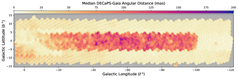
Figure 12: Median angular distance (NSide = 512) between source location in DECaPS2 and the crossmatched source location in Gaia eDR3. This figure employs a cut requiring that sources be brighter than $19$th magnitude in $g$-band and be detected three times (total, regardless of band).

To better contextualize DECaPS2, we show the spatial extent and overlap of other large-sky-coverage surveys (Figure 11). DECaPS2 fills a hole in coverage of the Galactic plane with deep ($r\sim 23^{\rm{rd}}$ mag) arcsecond resolution optical-NIR photometry.

The most comparable survey to DECaPS2 is Pan-STARRS1 (PS1) in the equatorial North (Chambers et al., 2016). PS1 uses similar filters ($grizy$) and reaches similar photometric depths (23.3, 23.2, 23.1, 22.3, 21.3 mag). On single-exposures, DECaPS2 is $\sim 1$ mag deeper than PS1, but contains fewer visits (3 versus 12). We engineered overlap with PS1 on both ends of the survey footprint (Figure 11) in order to cross-calibrate the surveys. Other optical surveys targeting the Milky Way disk include IPHAS (r, i, H$\alpha$) and VPHAS+ (u, g, r, i, H$\alpha$), which are roughly two magnitudes shallower than DECaPS2 in the overlapping photometric bands.

Other large programs on DECam include the Dark Energy Camera Legacy Surveys (DECaLS, Burleigh et al. 2020) and Dark Energy Survey (DES, Abbott et al. 2021) which provide $grz$ (24.7, 23.9, 23.0 mag) and $grizY$-bands (24.7, 24.4, 23.8, 23.1, 21.7 mag), respectively, at higher Galactic latitudes. The Legacy Survey footprint shown in Figure 11 includes both observations from DECam (declination less than +32°) and related programs observed from Kitt Peak National Observatory in the north. Smaller individual programs (including DECaPS1 data) on DECam were reprocessed as the NOAO Source Catalog (NSC) which fills the remaining optical-NIR hole in the equatorial South (see Figure 1 in Nidever et al. 2021).

The 2 Micron All-Sky Survey (2MASS, Skrutskie et al. 2006) can be used to probe further into the Galactic disk as a result of lower extinction from dust in redder wavelengths ($\sim 15.8,15.1,14.3$ mag depth in $J,H,K_{s}$). Targeted infrared plane surveys reach far fainter magnitudes ($K_{s}\sim 18^{\rm{th}}$ mag), such as the UKIDSS (Lawrence et al., 2007) Galactic Plane Survey (GPS, Lucas et al. 2008) and Vista Variables in the Via Lactea (VVV, Minniti et al. 2010; Saito et al. 2012; Alonso-García et al. 2018). In terms of longer wavelength space-based infrared astronomy, the Spitzer survey GLIMPSE (Benjamin et al., 2003; Churchwell et al., 2009) focused specifically on the Galactic plane ($\sim 18-17$ mag depth in bands 1-4) and the all-sky Wide-Field Infrared Survey Explorer (WISE, Wright et al. 2010; Schlafly et al. 2019) have imaged the Galactic plane at even longer wavelengths (20.7, 20.0 mag depth in W1, W2) where the effect of dust is even further suppressed.

6.1 Gaia

While DECaPS2 is primarily a photometric survey, it is important to have accurate astrometry in order to crossmatch between surveys. To evaluate the DECaPS2 astrometry, we match Gaia eDR3 sources (with a matching radius of 0.5”) to DECaPS2 and view the source locations in Gaia as ground-truth (Figure 12). We further require that the DECaPS2 sources be brighter than $19$th magnitude in $g$-band and be detected three times (total, regardless of band).

There is a clear, discontinuous change in the astrometry from a median error of $\sim 100$ mas in the center of the survey footprint to $\sim 18$ mas in the outer portion of the survey footprint. This is the result of changes in the astrometric reference catalog used by the DECam Community Pipeline (CP) as the survey progressed. At different points in the survey, the CP used 2MASS, Gaia DR1, or Gaia eDR3 to obtain the WCS solutions for a given CCD in an exposure. Since this astrometry is sufficient to match DECaPS2 to other photometric surveys, we take the heterogeneous astrometry from the CP without any further modifications. We do not attempt to resolve variations in the astrometry on the field-of-view scale visible at high Galactic latitudes because the magnitude of these variations are much smaller than the average astrometric precision over much of the DECaPS1 footprint. See Appendix D for more on the astrometric performance of crowdsource alone.

6.2 Pan-STARRS1

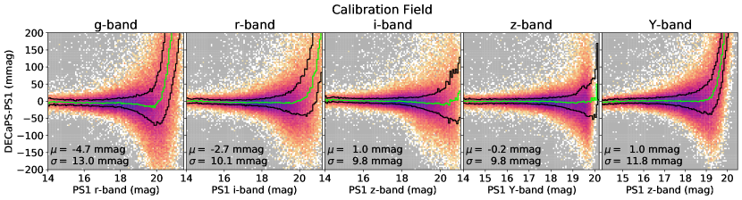
Figure 13: Comparison of DECaPS2 and PS1 catalogs on a low-extinction calibration field at ($\ell,b,\Delta\theta$) = ($236\degree$, $-14\degree$, $3\degree$), where $\Delta\theta$ is the angular radius of the circular field. The color scale is in log-density and each panel has its own normalization (light, white, low; dark, blue, high density). Lines indicate quartiles in the y-axis per x-axis bin with 25% and 75% in black and 50% (the median) in green. Outlier robust center (median) and scatter ($\sigma_{\rm IQR}$) metrics are shown for stars between $15^{\rm{th}}$ and $17^{\rm{th}}$ mag.

The absolute calibration of DECaPS2 was tied to PS1 by comparing a low-extinction calibration field at $(\ell,b)=(236\degree,-14\degree)$ in the overlap of both survey footprints (see Figure 11 and 13). The crossmatch for the figure required sources in PS1 to be within 0.5” of the source location in DECaPS2 and that there be no more than 1 match for a given source. We use a private reduction of PS1, available upon request. This catalog uses the original DR1 PS1 single-epoch detections, plus a somewhat more aggressive flagging of non-photometric and problematic detections than the public PS1 data. This reflects the catalog’s historical ties to the photometric calibration of PS1 (Schlafly et al., 2012), and is not expected to have any meaningful differences with respect to the public PS1 catalog for the kind of broad population-wide flux comparisons most relevant to DECaPS2.

We use the color transformation derived in the DECaPS1 paper on this calibration field to convert PS1 to DECaPS filters (Equation 2 in Schlafly et al. 2018). This transformation was obtained as a cubic polynomial fit to the color difference between DECaPS and PS1 bands as a function of the PS1 $g-i$ color. The zeropoint of that transformation was fixed by integrating HST-derived spectral energy distributions over the DECam and PS1 filter bandpasses, and thus ultimately derives from (Bohlin, 2014). We then adjust the absolute zeropoint of the DECaPS2 catalog to bring the fluxes measured in DECaPS2 into agreement with the color-transformed PS1 fluxes, for unsaturated point sources brighter than 17th mag in DECaPS. We show the spatial variation of this offset over the intersection of the DECaPS2 and PS1 footprints in Appendix E.

The median offset for stars $15^{\rm{th}}$ to $17^{\rm{th}}$ mag in PS1 is $<5$ mmag by construction of the absolute calibration. The median DECaPS2-PS1 magnitude difference is approximately flat down to $20^{\rm{th}}$ mag ($19^{\rm{th}}$ mag in $Y$-band). A sharp positive rise toward the faintest stars indicates that faint stars are estimated to be brighter in PS1 than DECaPS2. We attribute this to a selection effect given that the single exposure depth of DECaPS2 is $\sim 1$ mag deeper than PS1 (see Appendix F). Faint sources near the detection limit of PS1 are only detected if their flux fluctuates high via Poisson noise, but are not detected if they fluctuate low. Thus the PS1 flux will be overestimated relative to the true flux and the flux estimated by DECaPS2, since these sources are further from the DECaPS2 detection limit than the PS1 detection limit. In the bright limit, the scatter ($\sigma_{\rm IQR}$) between DECaPS2 and PS1 is $10-13$ mmag. This is a similar order of magnitude to the $10$ mmag uncertainty in the absolute calibration of PS1 and relative calibration of DECaPS2.

6.3 DECaPS1

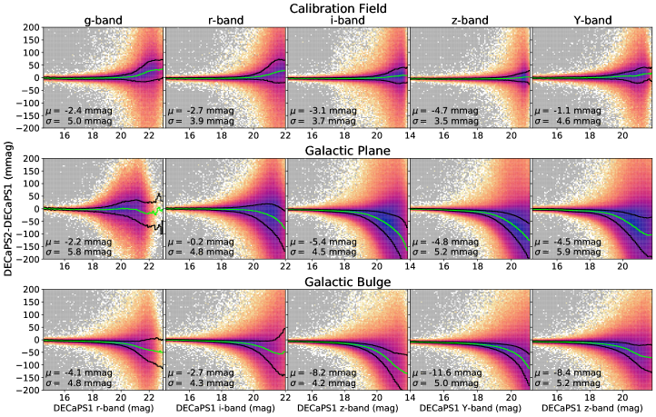
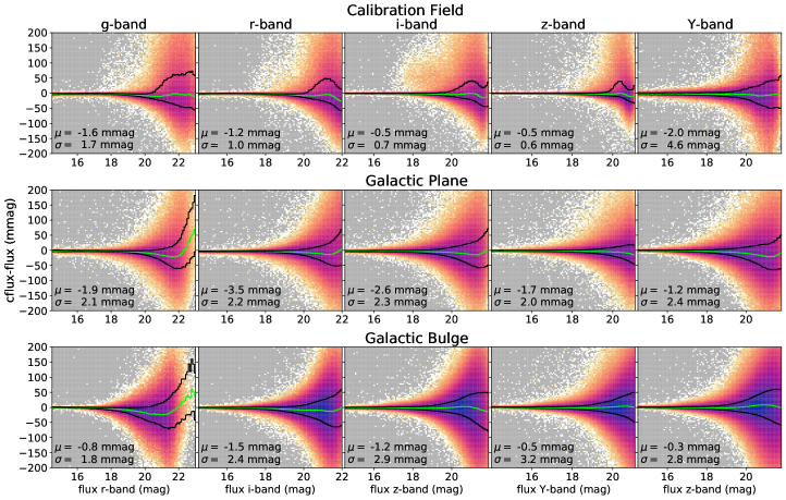
Figure 14: Comparison of DECaPS2 and DECaPS1 catalogs on three representative fields: in a low-reddening calibration field ($\ell,b,\Delta\theta$) = ($236\degree$, $-14\degree$, $3\degree$), in the Galactic plane ($\ell$, $b$, $\Delta\theta$) = ($-65\degree$, $0\degree$, $0.5\degree$), and in the Galactic bulge ($\ell$, $b$, $\Delta\theta$) = ($-5\degree$, $2\degree$, $0.5\degree$). $\Delta\theta$ is the angular radius of the circular field. The color scale is in log-density, and each panel has its own normalization (light, white, low; dark, blue, high density). Lines indicate quartiles in the y-axis per x-axis bin with 25% and 75% in black and 50% (the median) in green. Outlier robust center (median) and scatter ($\sigma_{\rm IQR}$) metrics are shown for stars between $15^{\rm{th}}$ and $17^{\rm{th}}$ mag.

Figure 15: Same as Figure 15 except comparing cflux - flux within the DECaPS2 catalog.

We also compare the new reduction to DECaPS1 on the overlapping footprint. This provides an internal consistency check on the relative calibration (which was performed independently for the DECaPS1 and DECaPS2 processing). The crossmatch required sources in DECaPS2 to be within 0.5” of the source location in DECaPS1 and that there be no more than one match for a given source. We show a comparison in all five bands for three representative fields in the Galactic plane, Galactic bulge, and at high Galactic latitude in Figure 15. The median offsets between DECaPS1 and DECaPS2 ($-5$ to $0$ mmag) computed using the bright stars ($15^{\rm{th}}$ to $17^{\rm{th}}$ mag) on the calibration field are artificially fixed by both surveys being calibrated to PS1 on that field.

However, the offsets for the Galactic plane and bulge fields are a quasi-independent check on the relative calibration for DECaPS data releases. The offsets observed ($-12$ to $0$ mmag) are again less than or equal to the absolute and relative calibration uncertainties ($\sim 10$ mmag). We attribute these offsets to the improved background estimation in the most recent version of crowdsource (see Saydjari & Schlafly 2022, in prep.), which enables sources to be more completely separated from the background. Since crowdsource iteratively finds sources, removes their flux, and recomputes a masked, moving-median background, it has a bias toward incomplete deblending (underestimating flux) for the faintest sources, which is exacerbated by worse background/PSF modeling. These offsets are typically at the $\sim 0.5-1\sigma$ level using the dflux per-object uncertainties. The scatter around the median for the DECaPS2-DECaPS1 crossmatch is at least a factor of two smaller than the DECaPS2-PS1 crossmatch. As expected, the scatter introduced by different processing and more data on the same instrument is smaller than the scatter comparing to a completely different photons measured by a different pipeline and instrument.

6.4 cflux

We also perform a consistency check on the background-corrected flux (Section 3.1.3) by examining cflux - flux as a function of magnitude on the same three representative fields in DECaPS2 (Figure 15). Systematic offsets in all plots are $<1\sigma$ using the dflux per-object uncertainties, and are more typically $\sim 0.25\sigma$. The median offsets on bright ($15^{\rm{th}}$ to $17^{\rm{th}}$ mag) stars are small, only $-3.5$ to $0$ mmag, but tend negative, indicating crowdsource is still not completely separating sources from the background. As expected, the largest fractional changes occur for the faint sources, which have comparable flux to diffuse background emission. These large relative changes lead to a larger scatter at faint magnitudes, as indicated by the larger separation between the 25% and 75% quartile lines. The faint interquartile range is much larger for the Galactic bulge and Galactic plane compared to the calibration field, which is expected given the much more complex structure of the background residuals which cflux corrects. Unlike the DECaPS2-DECaPS1 comparison, offsets for faint stars are in general small ($\sim 20$ mmag) and for the Galactic bulge and calibration field, have both signs. For the Galactic plane, all five bands dip slightly negative, indicating that the faint sources are estimated to be slightly brighter by cflux as compared to flux.

7 Injection Tests

While comparisons to other surveys provide helpful context and confirm consistency between different instruments or pipelines, it is important to evaluate the performance of a pipeline at recovering known sources– “synthetic injection tests.” We use these injection tests at the single-visit level to model the biases at low SNR. The single free parameter of our low SNR model is $s_{d}$, and we show in Appendix F that $s_{d}$ is related to the usual definition of photometric depth in terms of recovering 50% of sources at a given magnitude. Thus, we measure the photometric depth, including crowding effects and other complications via the observed low SNR bias. We further use the injections to evaluate the deblending performance of crowdsource and the accuracy of the reported flux uncertainties.

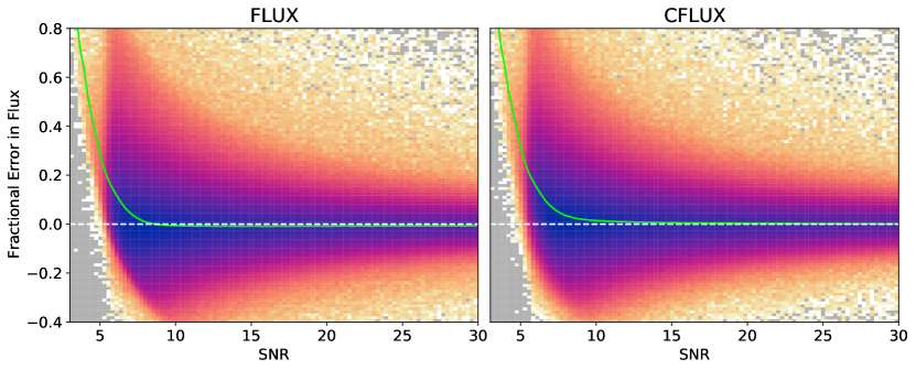
Figure 16: Histogram (2D) for injected source tests as a function of the “true” injected SNR ($s_{0}$) and fractional error in recovered flux using either flux (left) or cflux (right). Color scale is logarithmic density (light, white, low; dark, blue, high density) with gray indicating zero density. All panels include a cut selecting for unblended sources (see text). The green line shows the binned trimmed (excluding the highest and lowest 10%) mean as a function of SNR and the white-dashed line provides the zero-error reference.

To perform synthetic injection tests, we first obtain the photometric outputs for a given image, inject sources back into that image, and then solve the image with injections as if it were an additional CCD observed during that exposure. For each exposure in the survey, we select at random one CCD out of the $60-61$ observed CCDs per exposure on which to perform these injection tests. The density of injected sources is chosen to be $10\%$ of the source density in the original image, which we found to not significantly perturb the original solution.

We draw the flux of injected sources from the distribution of sources found in the original image, after excluding some sources. To prevent injecting very bright sources that will impact a significant fraction of the CCD area, we apply a strict cut on flux (in ADU) which corresponds to $\sim 17^{\rm{th}}$ magnitude in $g$-band. We also exclude sources from the seed distribution that have a “bad” flag set at their central pixel (saturation, broken pixel, etc.; see Table 5). We then sample sources from that flux distribution by uniform sampling of the linearly interpolated CDF. The source positions are drawn from a uniform (float, not integer) spatial distribution across the CCD, with a 33-pixel exclusion zone from the edges of the image.

The test sources are injected with the position-dependent PSF model obtained during the solution of the initial image. Injecting each source involves evaluating the PSF model at the injected location, an independent Poisson draw (consistent with the crowdsource gain) for each pixel in a stamp of pixels impacted by the star, and adjusting the weight image to account for the injected counts (again, consistent with the gain). We choose a stamp size of 511 pixels, which is much larger than the stamp size used to model most sources in crowdsource (19 or 59 pixels).

The image, weight image, and data mask (unchanged) after the injections are saved with RICE (lossy) compression to mimic the outputs of the CP. All random steps in our injection module use a PCG64 random generator seeded on the date-time in the filename of the exposure for reproduciblility. We save the locations and fluxes of the injected sources as an additional field in the catalog files (see Section 9).

One limitation of these injection tests is that the empirical flux distribution used for the flux draws may differ from the true flux distribution, especially near the faint end of the distribution. That is to say, the crowdsource outputs are incomplete for the faintest stars detected and thus the injections underestimate the number of faint stars to be injected. Another limitation is that injections use the crowdsource model PSF which may not match the true PSF for the image. However, these tests act as a consistency check on the model and provide a valuable measure of sensitivity in crowded fields.

7.1 Low SNR Bias

All survey pipelines have a limit below which they are unable to differentiate faint sources from noise. Using injection tests, we can characterize this limit and the biases resulting from the handling of faint sources. To first avoid the complexities of blending, we restrict our sample to sources injected at least 2 FWHM away from a source in the original image and found within 0.25 FWHM of the injected location. In rare instances, crowdsource can model the background as having negative counts or a source as having negative flux. We exclude both cases here.

We show in Figure 16 a (logarithmic) histogram of the fractional error in the flux recovered for injected sources over the entire survey footprint as a function of their injected signal to noise ratio (SNR). The green line shows the binned, trimmed (excluding the highest and lowest 10%) mean as a function of SNR. The white-dashed line provides the zero-error reference. The SNR is computed in the background-noise-dominated limit, assuming the PSF effective area is that of a Gaussian ($4\pi\sigma^{2}$), with the same FWHM as the source PSF.

$${\rm SNR}=\frac{f\times g}{\sqrt{4\pi\sigma^{2}\times b\times g}}$$ (7)

where $g$ is the crowdsource-estimated gain, $b$ is the background (in ADU) at the center of the source, and $f$ is the ground-truth flux of the injected source.

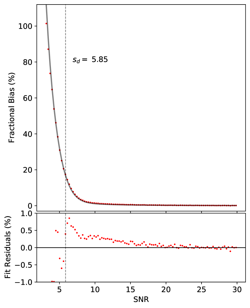
Figure 17: Average low SNR bias of cflux (red points) and least-squares fit to Equation 8 (gray solid line). The effective detection threshold of crowdsource obtained from the fit is shown (vertical gray-dashed line). Fit residuals are shown in the bottom panel.

When ambiguous, we denote this SNR by $s_{0}$ to distinguish it from SNR computed using the recovered flux $s_{r}$, the injected flux including the realization of Poisson noise $s_{i}$, and the SNR detection threshold of the photometric pipeline $s_{d}$.

The left and right panels of Figure 16 compare the recovered flux from crowdsource (flux) and the background-corrected flux from CloudCovErr.jl (cflux). The true flux is underestimated on average in the high SNR limit by flux at $-0.7\%$ (median for SNR 25-30). In contrast, cflux approaches zero bias from above (see discussion below) and is a $0.1\%$ overestimate over the same SNR range. A multiplicative underestimate of flux is in part expected for crowdsource since it sequentially detects and separates sources from the background. That is, until a source has been identified, the flux from that source contributes to the average that determines the background model. However, with each iteration (of which there are $4-10$), the flux estimate should converge to the truth from below. The background-corrected cflux likely detects this incomplete deblending relative to regions of pure sky and reapportions the flux from the background to the star.

The recovered flux is overestimated (positive bias) in the low SNR limit as shown by the positively diverging average (red line) in both panels. We explain (and model) this bias as resulting from two effects. For moderate SNR (10-20), a positive bias derived in Portillo et al. (2020) dominates, which results from using the maximum likelihood position for a source. Intuitively, this occurs because the maximum likelihood solution seeks to model as much flux as possible, even if that flux is partly background noise. This bias depends only on the true SNR of the source and an expansion to 4^th order gives the last two terms in Equation 8.

At low SNR, a detection bias dominates. In order to be found by crowdsource, the peak in the PSF-convolved image (after background subtraction) must be $5\sigma$ above the noise. Faint sources with noise that causes them to fluctuate high are found, but those that fluctuate low are not. This bias is reflected in the lack of sources in the lower left compared to the upper right of Figure 16.

In Appendix F, we derive a form of this detection bias which depends only on the true SNR of the injected source ($s_{0}$) and the source-detection threshold ($s_{d}$). Further, we apply an approximation to obtain the first term in Equation 8. This approximation is useful because it allows us to easily fit to the average bias from the injection tests and measure the effective $s_{d}$ of crowdsource.

$$\frac{\left<f-f_{0}\right>}{f_{0}}=\frac{B\left(\frac{s_{d}}{s_{0}}-1\right)}{1-e^{-\frac{A}{\sqrt{2}}\left(s_{d}-s_{0}\right)}}+\frac{1}{s_{0}^{2}}+\frac{1}{s_{0}^{4}}$$ (8)

Here (A,B) = (1.98, 1.135) are constants fixed by the approximation of the complementary error function ($\operatorname{erfc}$), $f$ is the measured flux, $f_{0}$ is the true flux, and $s_{d}$ is the single free parameter.

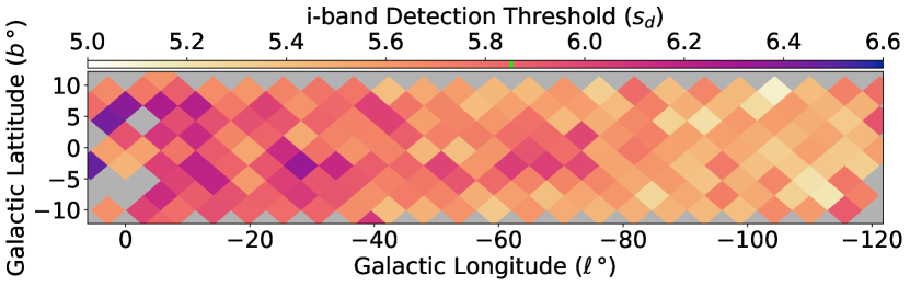
Figure 18: Spatial variation of the effective detection threshold $s_{d}$ in $i$-band, which tracks source density. The average value of $s_{d}$ obtained from the fit in Figure 17 is indicated on the color bar by a green line.

Figure 17 shows the weighted, least-squares fit of the average bias (red line in Figure 16) for cflux to Equation 8, using the square root of the number of sources per bin as weights. The optimal value for the effective source-detection threshold of crowdsource is $s_{d}=5.85$, which is higher than the formal $5\sigma$ detection threshold. The observation of $s_{d}>5$ is expected given the relatively local sky modeling and the fact that the local sky is biased high until a source is identified. The residuals are not trendless, but are $\sim 0.1\%$ in the high SNR limit and $\sim 1\%$ near the detection threshold. The remaining trend could result from the analytical approximations made to arrive at Equation 8, the use of a binned outlier-rejected average, the contribution of other unmodeled biases, or the breakdown of the background-noise dominated limit and the need to include the Poisson noise from the source.

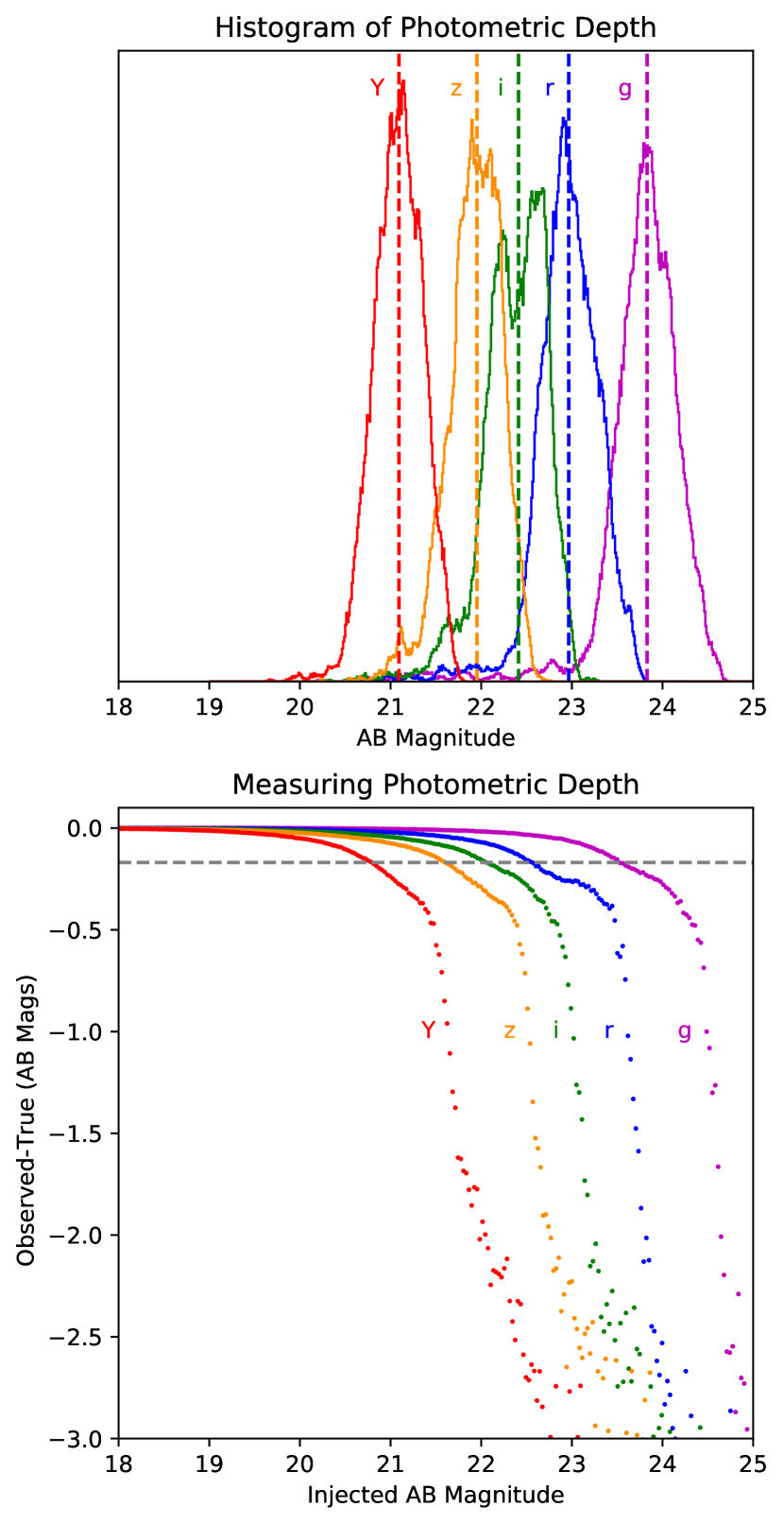
Figure 19: (Top) Histogram of imaging depth assuming 5.85$\sigma$-detection limit for each photometric CCD image included in the DECaPS2 catalog, separated by band. Dashed vertical line indicates the median. (Bottom) Median bias for recovered injected sources that are unblended as a function of magnitude, again separated by band. Horizontal dashed line indicates $-169$ mmag bias, which is the bias at which only $50\%$ of sources with that magnitude would be detected.

In the above fit, we have pooled over all injection tests over the survey footprint and over all photometric bands. However, variability in the background, source density, and PSF can change the effective detection threshold. In Figure 18, we restrict to $i$-band and perform the same fit as in Figure 17 to sources subdivided into NSide = 16 HEALPix pixels (about 2 degrees on a side). Only pixels with more than 900 sources passing the aforementioned cuts (to limit blending) are fit, which is why several pixels in the Galactic bulge are not treated by this analysis.

Despite the low resolution, there is a clear trend with source density–a lower detection threshold with lower source density, approaching the formal $5\sigma$ threshold. At higher source densities, $s_{d}$ approaches $\sim 6.5$. This could be a result of a larger density of real, below-threshold sources or the onset of blending effects. We exclude, at least partially, the effects of blending by a cut on sources in this plot, but have not accounted for the impact of blending on the bias model. Despite the variability shown in Figure 17, the average $s_{d}=5.85$ appears to adequately describe most of the survey footprint; we use this single value in what follows to avoid handling the Galactic bulge pixels which did not have enough isolated sources to estimate $s_{d}$.

These low SNR biases could be partially suppressed downstream of the single-exposure stage by using forced photometry at the average location of objects identified over different exposures and/or photometric bands. In that case, only sources with noise that fluctuates negative in every observation would be missed. However, no such post-processing is performed in DECaPS2. The catalog simply takes an average of all individual detections of an object (ignoring non-detections), which bakes in a positive detection bias. In order to implement a “correction” for the low SNR biases outlined above on a photometric catalog, we would need to use a prior on the true source-flux distribution. Choosing a prior would allow a statistical correction as a function of the observed SNR. We leave individual use cases to decide on the appropriate prior and here simply use the bias to inform the quality of our photometry.

7.2 Photometric Depth

One of the most important metrics of a photometric survey is its depth, often defined as the magnitude such that $50\%$ of sources with that flux are recovered. One way to estimate this metric is to assume a recovery limit in SNR for the photometric pipeline, which we will choose to be 5.8 as informed by the fit above. Then, using the gain, average PSF width, and average sky counts for a CCD, we can use Equation 7 to solve for the equivalent flux. Accounting for the variable zeropoints per exposure and only including photometric exposures that are used in creating the catalog, we obtain Figure 19 (top). The histogram of depths spans roughly $\pm 1$ mag. The strong bimodality in $i$-band is the result of brighter-than-usual sky during the beginning of the DECaPS1 observing run.

In light of Figure 16, calculating photometric depth by fixing an SNR detection limit (without using injection tests to determine $s_{d}$) is only marginally more accurate than choosing the depth based on the turnover in the magnitude histogram for recovered sources. While it might be attractive to use injection tests to determine at what magnitude $50\%$ of injections are recovered and define that as the depth, such a definition is strongly sensitive to how one defines a source as being correctly recovered. How close is the source to the injected position and, even more importantly, how close is the recovered flux to the true injected flux? These questions are significantly complicated by blending in crowded fields and the bias shown in Figure 16.

Instead, we can use the injections to measure the achieved survey depth based on the observed low SNR bias. As shown in Appendix F, it turns out that $s_{d}$ is exactly the SNR ratio such that a $s_{d}$ source has a $50\%$ chance of recovery in a given exposure. Then, once $s_{d}$ is known, we can find the fractional bias at $s_{d}$, 16.9% for $s_{d}=5.85$ (see Appendix F). Since we often consider differences in magnitudes, we can convert from fractional error to obtain a bias of $-169$ mmag. By measuring at what calibrated magnitude the recovered injection tests are biased by $-169$ mmag, we measure the effective photometric depth of the survey, including crowding effects and other complications.

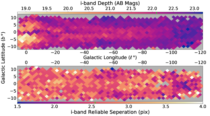
Figure 20: Variation of the photometric depth (top) and reliable separation (bottom) in $i$-band across the survey footprint. Both are determined by a threshold of $-169$ mmag bias on recovered injected sources. The average depth from Figure 19 and the median reliable separation over the survey footprint are indicated on the respective color bar by a green line.

Using the same cuts to obtain only well-separated sources as in Figure 16, we obtain Figure 19 (bottom). For each photometric band, we show the median bias for the recovered flux in a narrow magnitude range as a function of the magnitude of the injected source. The onset of a positive bias is observed toward the faint limit and the intersection of the median curve with the $-169$ mmag threshold (gray, dashed) determines the limiting magnitude in that band.

Using the bias method, we find the photometric depths are 23.5, 22.6, 22.1, 21.6, 20.8 mag in grizY bands, respectively. These depths are usually slightly brighter ($\sim 300$ mmag) than using the median of the histograms assuming a sharp SNR cutoff which give depths of 23.8, 23.0, 22.4, 22.0, and 21.1 mag. Using either method, these depths surpass the targets (24.1, 22.3, 21.2, 20.6, 20.3 mag; see Section 2) in all bands but $g$-band, which is a 0.5 mag shallow. However, we have three images in each band, so even in $g$-band, a future processing that coadds images would reach our target depth.

Another benefit of the bias method on injections is that we can map spatial variations in the depth (available in Section 9) at a spatial resolution set by the injected source density (Figure 20, top). To do so, we no longer apply the cuts restricting to unblended sources in order to measure the depth in the Galactic bulge. We observe spatially correlated variations across the survey footprint for $i$-band, which clearly track source density. The survey is $\sim 1$ magnitude deeper at high latitude and in regions of low source density and $\sim 1-2$ magnitudes shallower toward regions of high source density. In the Galactic bulge, some of this bias likely derives from blending, but in the crowded field limit where depth is difficult to define, it is desirable to have the depth track the reliability (bias) of sources as a function of magnitude.

7.3 Blending

We can also use injection tests to provide a measure of a reliable separation at which sources are correctly deblended by crowdsource. We can measure the maximum separation between the injected source and a source in the original image before the source is biased more than a threshold. Here we again choose a $-169$ mmag bias threshold, but here it just serves as a well-motivated measure of when the blending bias becomes “significant,” as measured relative to the detection bias at threshold. The variation of this “reliable distance” in pixels (which are 0.26” for DECam) is shown over the survey footprint in $i$-band in Figure 20, bottom. We consider only injections within 8 pixels of an original source and only show HEALPix NSide = 32 pixels with more than 200 such sources.

There is a sharp cut preventing source deblending below one pixel in crowdsource. At low source densities, crowdsource appears to approach this limit with reliable deblending distances of $\sim 1.5-1.7$ pixels. However, for much of the survey footprint, the reliable separation is closer to 3 pixels. Taking a median over the survey footprint, we find an average reliable separation of 3.0, 2.9, 2.5, 2.5, 2.5 pixels and median FWHM of 5.2, 4.8, 4.4, 4.2, 4.1 pixels for $grizY$, respectively. This suggests the median performance is deblending sources separated by $\sim 60\%$ of the FWHM, which is better than the Rayleigh resolution limit. These measures are complicated in part by the variations in the underlying source-density distribution which can modify the observed bias.

We further investigate the onset of bias from blending using the injection tests in $z$-band in Figure 21. In the top left, we apply the cut to consider only unblended sources and show the median Z-score as a function of the (log₁₀) injected SNR for both flux and cflux. For sources over 10 SNR, the median Z-score is approximately flat with respect to injected SNR. The remaining trends observed could arise from the discrete changes in size of the PSF stamp used by crowdsource to model sources. For cflux the median Z-score is centered around zero, while flux is biased low by $-0.1\sigma$, in agreement with Figure 16. Below 10 SNR, sources are biased high for reasons described in Section 7.1.

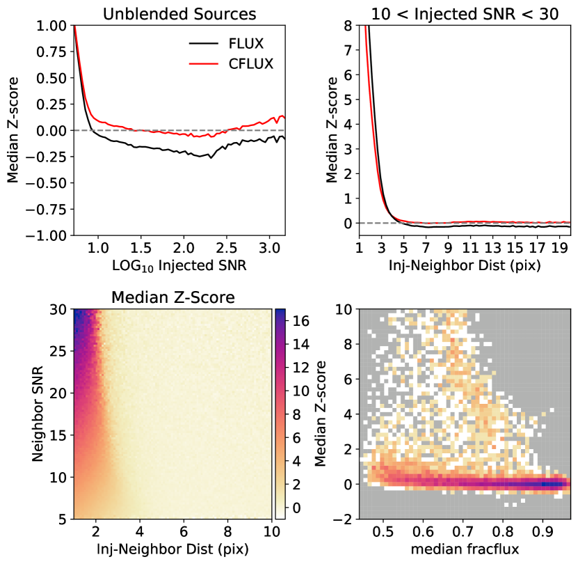
Figure 21: (Top Left): Median Z-score for unblended, injected $z$-band sources as a function of the injected SNR for both flux and cflux. (Top Right): Median Z-score for injected sources with moderate SNR as a function of distance to a source in the original image. (Bottom Left): Additional dependence on the neighbor SNR is shown. (Bottom Right): Converts the bottom left panel into a 2D histogram of the median Z-score bias versus the median fracflux for the given injected-neighbor source distance. Color scale is logarithmic density (light, white, low; dark, blue, high density) with gray indicating zero density.

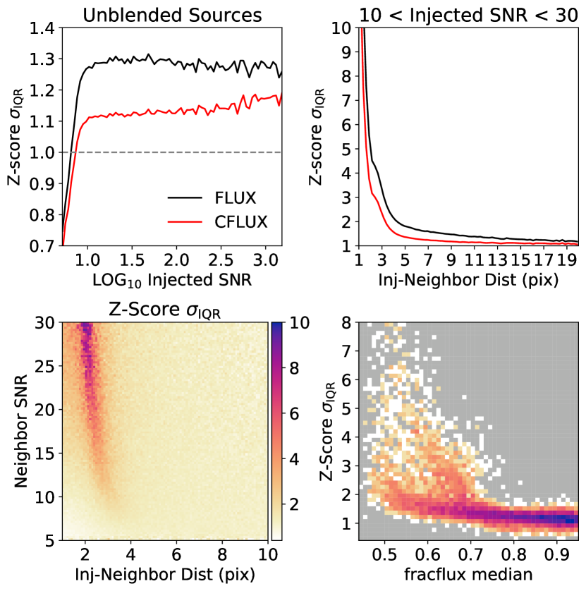
Figure 22: Same as Figure 21 for Z-score $\sigma_{\rm IQR}$ instead of the median Z-score.

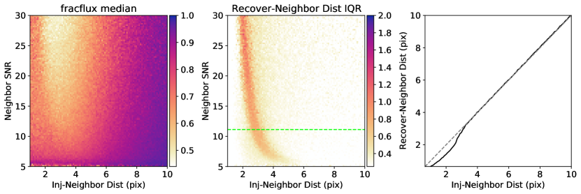
Figure 23: (Left): Median fracflux as a function of the neighbor SNR and distance between the injected source and neighbor. (Middle): IQR of the distance between the recovered location for an injection and the nearest neighbor on the same axes. (Right): Line cut along the green-dashed line in the middle panel showing the median distance between the recovered location for an injection and the nearest neighbor versus the between the true injected location and the nearest neighbor. Perfect location recovery would fall along the 1:1 line (gray, dashed).

The additional bias introduced by blending is shown in Figure 21, top right, where the $z$-band sources are such that flux is positive, the background model is positive, and the source is found within $0.25$ FWHM of the true injected location. The injected sources are further limited to moderate SNR injections, those with injected SNR between $10$ and $30$. The median Z-score diverges as the distance to a source in the original image decreases, making 1$\sigma$ errors at $\sim 3$ pixel separations and $>5\sigma$ errors at $\sim 2$ pixel separations and below. At the smallest separations, we expect the injected and original source are confused and merged into a single detection. While the cflux Z-scores diverge more slowly, CloudCovErr.jl makes no attempt to account for blending.

The impact of blending also depends on the flux of the blended neighbor. Continuing to restrict to moderate SNR injections, the bottom left of Figure 21 shows the median Z-score as a function of both the distance to the nearest source in the original image and the SNR of that neighboring source (which is proportional to flux). If the neighbor SNR is a similar order of magnitude to the injected source, a bias is introduced at small separations that increases with increasing neighbor flux. There is a sharp onset of this bias around $2-3$ pixel separations with a trend that will be discussed below. If the neighbor SNR is very large relative to the injected source, the injected source will not be found if it is too close (further up the vertical axis, not shown). However, in the limit of the smallest separations, the injected source will be recovered regardless of the neighboring SNR, just as a very biased source which has a flux that is the sum of the two sources (far left edge of the plot).

In the bottom right of Figure 21 converts the bottom left panel into a 2D (logarithmic) histogram of the median Z-score bias versus the median fracflux for the given injected-neighbor source distance. For all fracflux $>0.5$, the vast majority of Z-scores are $\leq 1$, with a trend of increasing bias toward more blended sources (lower fracflux). There is an onset of $>5\sigma$ errors at $\texttt{fracflux}=0.75$. The outliers above $\texttt{fracflux}=0.75$ are the result of close ($<3$ pixel separation) sources with fainter SNR than the injected source ($<10$). Since the recovery fraction of such sources near the detection threshold is low, similar levels of bias from undetected sources is possible. In the bottom panels of Figure 21 and 22, we show results for cflux. The equivalent plots for flux are qualitatively the same, but have biases $1.5-2$ times larger.

In addition to measuring bias, injection tests can be used to measure if the reported photometric uncertainties accurately capture the errors made by the photometric pipeline. Figure 22 shows this analysis in the context of blending, with cuts mirroring those in Figure 21. If the error bars were exactly correct, the Z-score distribution for recovered sources would be a unit normal distribution with $\sigma_{\rm IQR}=1$.

The $\sigma_{\rm IQR}$ of the Z-scores for unblended sources as a function of the injected source SNR is shown in the top left of Figure 22. Above SNR 10, the $\sigma_{\rm IQR}$ is approximately flat with respect to SNR. Using flux (and its associated uncertainty), the $\sigma_{\rm IQR}$ is $\sim 1.3$ times larger than the normal value, indicating that the flux uncertainties are underestimated. For cflux, the uncertainties are closer to correct and lead to an $\sigma_{\rm IQR}$ only $\sim 1.1$ times larger than the normal value. This is in part expected since the associated uncertainties with cflux account for the off-diagonal correlations in the background model, in additional to the usual diagonal Poisson contributions, when computing uncertainties.

Blending complicates the estimation of uncertainties but is not explicitly accounted for by either flux or cflux. This is illustrated in Figure 22, top right, where the Z-score $\sigma_{\rm IQR}$ diverges as the distance to a source in the original image decreases, underestimating the error bars by a factor $3-5$ at the separations on the order of a two pixels.

The bottom left of Figure 22 shows that if the neighbor SNR is small relative to the injected source, there is almost no measurable impact on the recovered Z-score $\sigma_{\rm IQR}$ of the injected source at any distance. In the limit where the sources are close together, they are not deblended and the injected source is simply recovered as having the sum of the fluxes for both stars. This merging of the sources shows up as a bias (see Figure 21), but does not impact the $\sigma_{\rm IQR}$. In between the well-separated and merged limit, there is up to an order of magnitude underestimation of the uncertainty. This “deblending” uncertainty derives primarily from the variability in the number of sources used to model the injection and neighbor (1 or 2 sources) and the source location, as shown in Figure 23. Accounting for “deblending” uncertainty correctly in large-scale photometric pipelines is an important remaining challenge for the field, for which tests similar to the one above can be diagnostic.

The bottom right of Figure 22 converts the bottom left panel into a 2D (logarithmic) histogram of the Z-score $\sigma_{\rm IQR}$ versus the median fracflux for the given injected-neighbor source distance. Above $\texttt{fracflux}=0.75$, the distribution of $\sigma_{\rm IQR}$ is tight and flat near 1. Below $\texttt{fracflux}=0.75$, outliers with $\sigma_{\rm IQR}$ $>3$ appear and the overall tilt toward increasing $\sigma_{\rm IQR}$ with decreasing fracflux becomes more pronounced. The left panel of Figure 23 shows the median fracflux as a function of the neighbor SNR and injection-neighbor distance. This reaffirms that sources past the peak in Z-score $\sigma_{\rm IQR}$ are often merging with the neighboring source, leading to an increase in the fracflux with decreasing separation. While the lowest fracflux for a given neighbor SNR does coincide with the peak in Z-score $\sigma_{\rm IQR}$, the shape of the change in fracflux is much broader.

The middle panel of Figure 23 shows the variability (IQR) in the distance between the location at which the injected source is recovered and the location of the neighbor in the original image. In the ideal case, this variability would be zero with the injected source location being recovered at the true location every time. However, there is a sharp peak in the variability of the distance between the recovered location and the neighbor, which matches the peak in Z-score $\sigma_{\rm IQR}$.

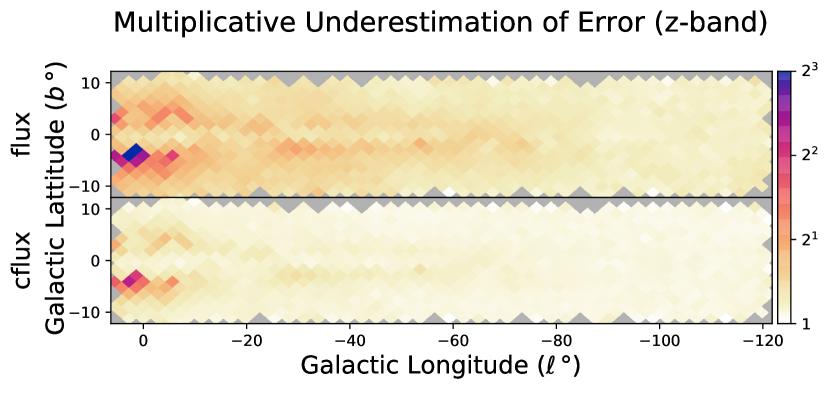
Figure 24: Color map of the multiplicative underestimation of error as measured by $\sigma_{\rm IQR}$ for $z$-band flux and cflux over the survey footprint. The color scale is $\log_{2}$ to emphasize the large range of values while maintaining interpretability. Top and bottom compare results for flux and cflux, respectively.

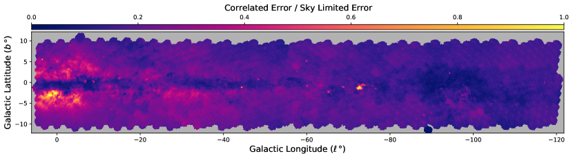
Figure 25: The ratio of the additional uncertainty CloudCovErr.jl introduces as the result of correlations to diagonal Poisson uncertainty from the background sky counts (Equation 9), shown over the survey footprint. Each HEALPix pixel shows an outlier-clipped mean with a further requirement that sources have the CloudCovErr.jl flag dnt == 0.

To further clarify the nature of this peak, the right panel of Figure 23 shows the median distance between the recovered location and the neighbor versus the distance between the true injection location and the neighbor, for fixed neighbor SNR (slice along green-dashed line). In the ideal case, these two distances are the same and the data would follow the 1:1 line (diagonal dashed gray) as they do for all separations above $3.5$ pixels. At the onset of the peak in distance and Z-score $\sigma_{\rm IQR}$, the distance between the recovered location and the original source shows a large decrease below the true value, which persists at lower separations. Thus, the uncertainty estimates for the source flux fail most catastrophically when the source location is being pulled toward its neighbor and the pipeline finds the number of sources ambiguous.

A tilt in the peak in the distance IQR illustrates the intuition that bright sources must be closer together before it is difficult to determine if there is one source or two sources close together. Below an SNR of $10$, this tilt gains curvature, suggesting that faint sources near the detection threshold are absorbed into the injected source at much larger separations. However, there are some selection effects at play in the sample in Figures 21, 22, and 23. The figures are not sensitive to the case where the injected source is not detected within $0.25$ FWHM from the injected location, because its flux is either totally absorbed by the original source (without shifting the original source location significantly) or its location is shifted by more than $0.25$ FWHM by the presence of the original source.

7.4 Validating Uncertainties

To avoid these complications associated with blending, but still make a map of the spatial variation (available in Section 9) in the quality of our flux uncertainties, we again limit to unblended injected sources and further limit to $\log_{10}$ injected source SNR between $1.1$ and $3.2$, where Figure 22 (top left) is approximately invariant to the injected source SNR (Figure 24). For flux, the median multiplicative underestimation of error over the survey footprint is $1.3$, and tracks source density as illustrated by the large $\sigma_{\rm IQR}$ in the Galactic bulge and just off the Galactic plane. For cflux, the median multiplicative underestimation of error is only $1.1$ and improves the $\sigma_{\rm IQR}$ in bulge by factor of two. This comparison illustrates that while cflux does deliver the intended improvements to background modeling, neither flux nor cflux handle blended-source uncertainties well. This should be a focus of future development for pipelines in crowded fields. For now, the map in Figure 24 can act as a suggested multiplicative correction to the reported uncertainties in DECaPS2.

8 Astrophysical Tests

Another useful set of tests is to evaluate the performance of our photometric reduction on astrophysical targets where we have prior knowledge that informs an expected result.

8.1 Nebulous Uncertainties

The main purpose of the CloudCovErr.jl processing is to improve the uncertainty estimates in regions with structured backgrounds by including off-diagonal terms in the covariance matrix. Thus, we want to confirm that CloudCovErr.jl is increasing the uncertainties predominately in regions of the Galaxy with known nebulosity. Figure 25 shows the ratio of the additional uncertainty that CloudCovErr.jl introduces as the result of correlations to diagonal Poisson uncertainty from the background sky counts.

$$\frac{\rm{Correlated\,Error}}{\rm{Sky\,Limited\,Error}}=\frac{\sqrt{\texttt{dcflux}^{2}-\texttt{dflux}^{2}}}{\sqrt{4\pi\sigma^{2}\times b\times g}}$$ (9)

We report an outlier-clipped mean value of the ratio for stars within each HEALPix pixel. The outliers are values beyond 10*$\sigma_{\rm IQR}$ and are computed per CCD. In addition, we require the CloudCovErr.jl flag dnt = 0.

This measure provides a relative scale for the magnitude of these correlations and is robust to variations in the sky brightness, seeing, and the distribution of source fluxes. However, the qualitative features are similar to those observed by simply taking a ratio of the cflux and flux uncertainties (dcflux and dflux), which was shown in Figure 13 of Saydjari & Finkbeiner (2022).

Overall, the correlated uncertainties track source density, are $\sim 0.5$ times the sky-limited flux uncertainty just off the plane $\ell<-40\degree$, and can be larger than the sky uncertainty in the (Southern) Galactic bulge. The peak associated with the Carina Nebula ($b=-0.8\degree,\ell=-73\degree$) and filaments associated with the Vela supernova remnant ($b=-2.8\degree,\ell=-96\degree$) show that the correlated uncertainties are sensitive to structured backgrounds as intended. Other point sources correspond to known nebulae, globular clusters, or artifacts in the background near very bright stars. Thus, the behavior of dcflux on the structures present in the survey footprint agrees with our prior knowledge.

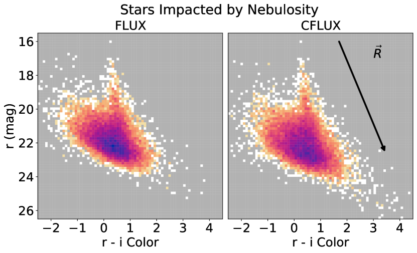
Figure 26: CMD in $r$ versus $r-i$ using flux (left) and cflux (right) for selected sources near the Vela supernova remnant impacted by nebulosity (see text for exact cuts). Color scale shows log density (light, white, low; dark, blue, high) on a common scale. Reddening vector (right) showing effect of dust plotted for reference. cflux shifts stars with overestimated $r$-band flux toward a simple reddened main sequence.

8.2 Nebulous CMD

To test performance of the photometry in the presence of nebulosity, we target a radius $4\degree$ region ($264.6\degree$, $-4.8\degree$) near the Vela supernova remnant which has significant filamentary H$\alpha$ emission (appearing in $r$-band). We further limit to the stars most impacted by the sparse filaments by requiring in both $r$ and $i$-bands that:

• the off-diagonal contributions to the uncertainty be large, dcflux-dflux $>10^{-10.5}$ Mgy

• the nebulosity correction to flux be large (and negative), flux - cflux $>10^{-10.5}$ Mgy

• no dnt flags are thrown for any detections

We show the CMD in $r$ versus $r-i$ of this sample in Figure 26 using both flux (left) and cflux (right) for comparison. Given our knowledge of stellar evolution, we have an expectation that the CMD (for stars in this region of the disk) is dominated by the main sequence (straight vertical), with a tilt as a result of reddening from dust. The cflux CMD more closely resembles that expectation. The cflux CMD shifts weight from the blueward tilted population at fainter magnitudes, caused by overestimation of the $r$-band flux, toward the main sequence and along the reddening vector. The sample size here is limited by the density of sources on the edge of a filament in an evolutionarily simple region, which is why repeated injection tests in filamentary regions are valuable (see Figure 10, Saydjari & Finkbeiner 2022).

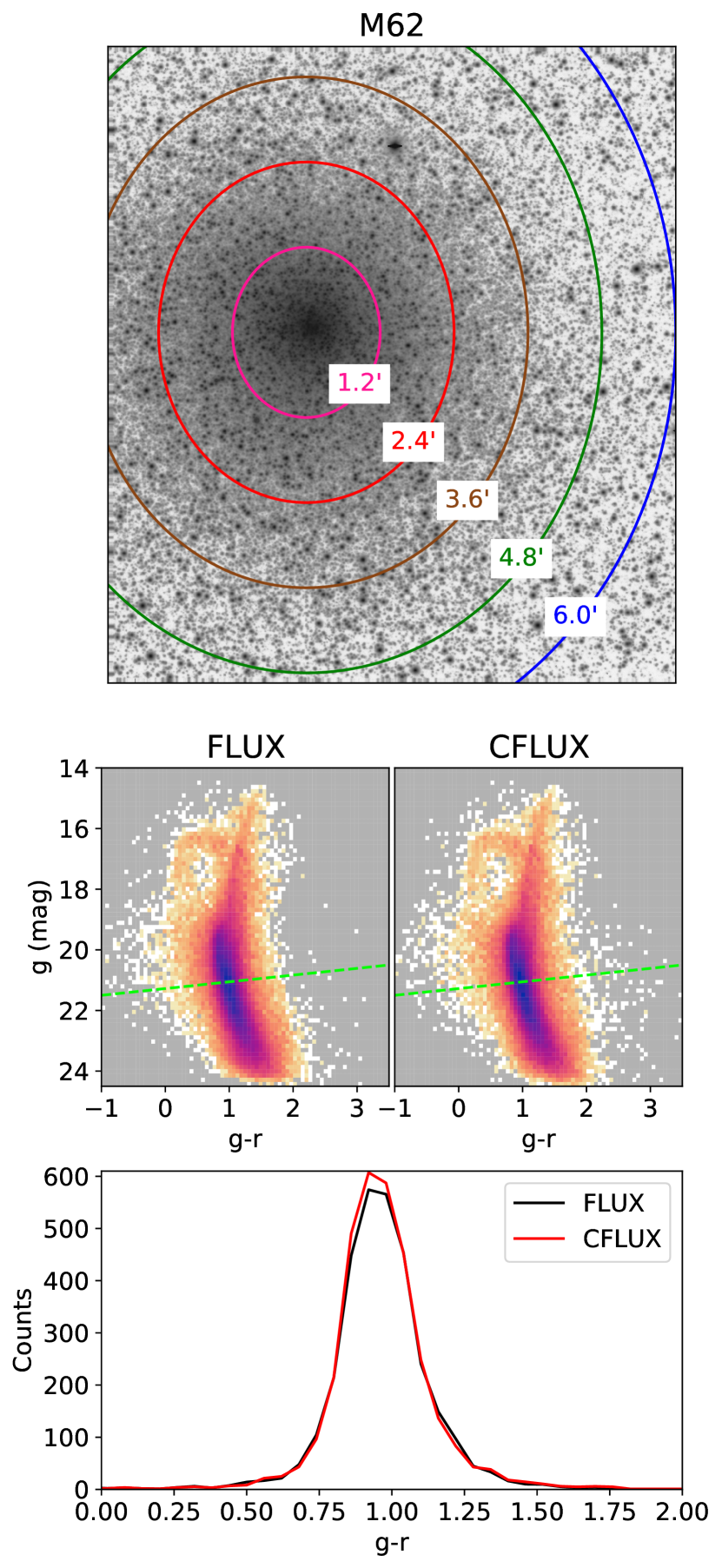
Figure 27: (Top) Single-exposure $g$-band image of M62 with labeled radii in steps of $1.2^{\prime}$. Color scale is $\operatorname{arcsinh}$ stretched around the median with high and low counts in black and white, respectively. (Middle) CMD in $g$ versus $g-r$ for all sources within $6^{\prime}$ of the center of M62 using flux (left) and cflux (right). Color scale shows log density (light, white, low; dark, blue, high) on a common scale. (Bottom) Line cut along the green-dashed line in middle panels showing the sharper main sequence given by cflux.

8.3 Globular Cluster

Globular clusters, which are formed from only one (or a few) star-forming episodes, are useful reference objects because they act as snapshots at fixed stellar age. In addition, they also provide a gradient of source densities, with some of the densest, hardest to deblend regions at their centers.

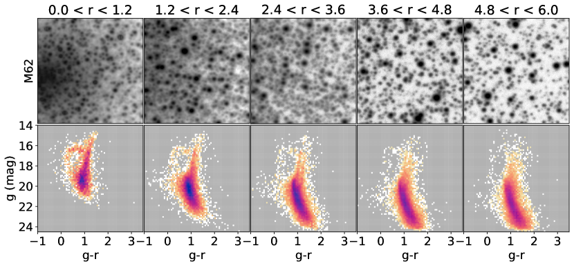
Figure 28: (Top) Image ($g$-band) stamps cut from annuli around M62 between the indicated radii. Each image is $\operatorname{arcsinh}$ stretched around the median with its own color scale (black high and white low counts) to emphasize the increasing degree of blending toward the center of the globular cluster. (Bottom) CMDs in $g$ versus $g-r$ for sources found in the indicated annuli. Color scale shows log density (light, white, low; dark, blue, high) on a common scale in units of sources per square-degree.

We consider M62, the brightest globular cluster (6.45 V mag) in the DECaPS2 survey footprint, as an example (see Figure 27, top). We show the CMD using both flux (middle left) and cflux (middle right) in $g$ versus $g-r$ for all sources within $6^{\prime}$, which is about 60% of the tidal radius. The CMD using cflux is slightly sharper around the main sequence track which agrees with our expectation that there should be little to no metallicity scatter. Line cuts transverse to the main sequence are shown in the bottom panel for emphasis. Importantly, the bias-variance trade-off inherent in any bias correction such as that used for cflux does not add so much scatter as to obscure finer features visible for the globular cluster, such as the blue horizontal branch (curved feature near 16^th magnitude).

Globular clusters also act as a test bed for the performance of deblending algorithms. We subdivide M62 by radius in steps of $1.2^{\prime}$, as indicated in Figure 27. In Figure 28, we show the CMD in $g$ versus $g-r$ for sources in each annulus and an example image cutout to demonstrate the degree of blending in that field. In the largest annulus, we recover sources brighter than $24^{\rm{th}}$ mag. Closest to the center, the crowding is so significant that only sources brighter than $\sim 21^{\rm{st}}$ are recovered. In all cases, the recovered CMDs appear to be differently weighted samplings of the same underlying CMD. This is the desired behavior for when a deblending algorithm encounters a field more blended than it can deconstruct; the detection limit moves to a brighter level, but the sources identified are still of science quality.

9 Data/Code Availability

Data products associated with DECaPS2 are publicly available on the survey website http://decaps.skymaps.info/. We provide a data model (inspired by SDSS) that documents the contents and structures of all released files. We provide single-epoch catalog outputs from both crowdsource and CloudCovErr.jl, the final object-merged catalog as subdivided FITS files for flexible database ingestion, and files that specify the zeropoints and photometric cuts from the calibration. We build and store the merged catalog using the Large Survey Database and make those tables available.

Raw images in addition to the InstCal processed images used here are available from the NOIRLab Archive. Since there are multiple versions in the NOIRLab Archive for a subset of the images which required reprocessing by the DECam Community Pipeline, we also provide the exact list of InstCal processed images that we used to create DECaPS2 for the sake of reproducibility.

Work on the DECam Community Pipeline is led by F. Valdes and source code is available by request, but documentation and support for use is limited. crowdsource is publicly available on Github and is distributed via condaforge. CloudCovErr.jl is publicly available on Github and is distributed through the Julia package registry. A Jupyter notebook with the code and data compilations necessary to reproduce all figures in the text are available on Zenodo at doi:10.5281/zenodo.6677609.

10 Conclusion

With DECaPS2, we provide deep optical-NIR ($g\sim 24$th to $Y\sim 21$st mag) coverage of the southern Galactic plane (6.5% of the sky) with approximately 1” seeing. Combined with PS1, this completes comparable imaging of the entire Galactic plane essential for probing our Galaxy’s stars, gas, and dust. We use crowdsource to process images and create a catalog with 3.3 billion objects built from 34 billion detections. The relative photometric calibration is uniform and has a precision of $\sim 7$ mmag, with an absolute calibration tied to PS1.

A detailed analysis of detection quality metrics and crowdsource failure modes led to improved quality cuts, which were applied in creating the object catalog. Given that fracflux is a common quality cut used on the object catalog, we provide guidance for a threshold on fracflux (which is extremely conservative). We compare the DECaPS2 astrometry to Gaia and DECaPS2 photometry to both PS1 and DECaPS1, showing strong agreement and internal consistency. A similar comparison validates our new background-corrected flux, cflux, produced by CloudCovErr.jl. The performance of the convolutional neural network (CNN) that identifies nebulosity and modifies the deblending in crowdsource was validated by correct identification of Galactic nebulosity over the survey footprint.

We performed synthetic injection tests over the entire survey footprint and used them to measure and model the biases for low SNR sources. This bias was leveraged to empirically measure the photometric depth of the survey. Through injection tests, we also quantify the deblending performance of crowdsource and find uncertainties to be underestimated when the number of sources is ambiguous. We make a map of the multiplicative underestimation of error bars across the survey footprint, which can be used in downstream statistical analyses and which illustrates the improvement of cflux over flux. Further, we use astrophysical priors on nebulous regions of the Galaxy and globular clusters to further validate the deblending performance of crowdsource and the correction introduced by CloudCovErr.jl.

All images, single-visit catalogs and models, and combined source catalogs are publicly available and well-documented by a data model. These well-validated data products with many quality flags (even beyond those explored in detail here) should provide a rich, adaptable resource for the community, facilitating a variety of studies of the Milky Way galaxy. We look forward to using DECaPS2 to refine dust reddening models and as a photometric input for the statistical inference of the 3D distribution of dust in the Milky Way, probing further into the Galactic plane.

Appendix A PSF FOV Variation

DECam, as with any optical system, has a variable pixel scale across the wide field of view resulting in a variation of the PSF. A variable pixel scale would result in a photometric variation if not for the flat fielding corrections. In Figure 29 we show the FWHM in pixels for sources from crowdsource as a function of position on the focal plane of a typical $g$-band exposure. There is a clear, asymmetric increase in the FWHM toward the edge of the field of view, larger toward the western edge (right side of plot).

We have not isolated that source of this variation to either an instrumental effect or a stage in the CP-crowdsource pipeline and the origin of this variation remains an open question. However, the pattern of PSF FWHM variation shown in Figure 29 appears related to the pattern noise in the average fracflux (Figure 8).

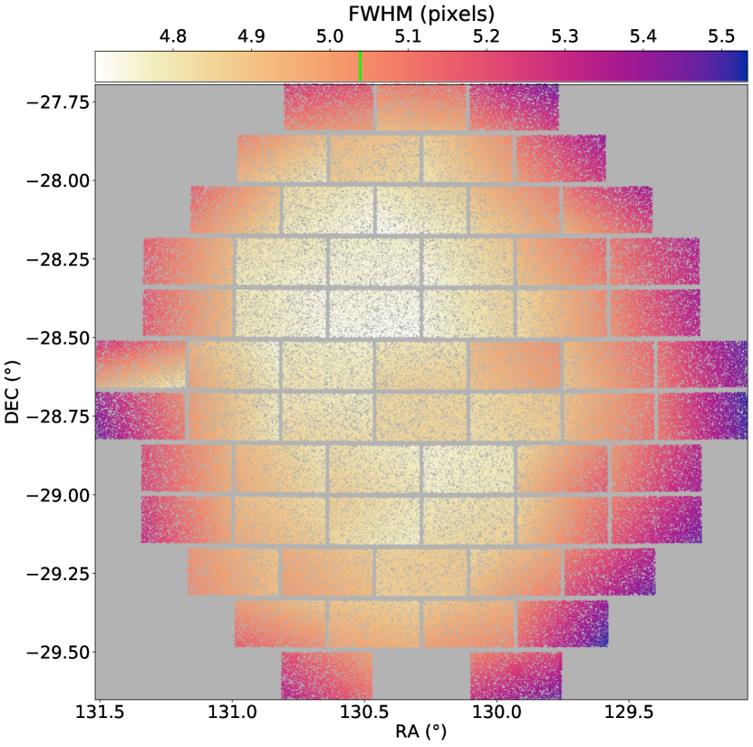
Figure 29: The FWHM for sources from crowdsource as a function of position on the focal plane of a typical $g$-band exposure. The median $g$-band FWHM reported for the whole survey is indicated on the color bar by a green line. The sky orientation shown for the focal plane is north up, west right.

Appendix B CCD Saturation Thresholds

At some point between Run 12 and 13 (see Table 2) the (software) saturation thresholds in the CP changed. This change left pixels at or near saturation unmasked for several CCDs. Since the 200 brightest “unsaturated” stars, stars without pixels flagged by the CP as saturated, are used for PSF fitting in crowdsource, the PSF crowdsource learned and used to measure the photometry of the affected CCDs was distorted. This unfortunately impacted all of the photometry for a given CCD, not just the measured fluxes of the stars near saturation. In most cases, making a logarithmic histogram of the per pixel counts revealed a “pile-up”, the beginning of which could be used to define the onset of saturation. However, a few cases required even lower thresholds.

When the saturation threshold for a given CCD is set too low, the $\hat{\chi}^{2}_{r}$ from crowdsource of the few brightest stars will be anomalously high because while the stars are unmasked, they are actually at/near saturation and thus distorted relative to the true PSF. We then used the ratio of the average $\hat{\chi}^{2}_{r}$ for the few brightest stars and the average $\hat{\chi}^{2}_{r}$ of bright stars far from saturation as an indicator for CCDs needing a saturation threshold adjustment (Figure 30). Only the saturation threshold for CCDs that were consistently flagged across multiple exposures and bands were adjusted (list in main text).

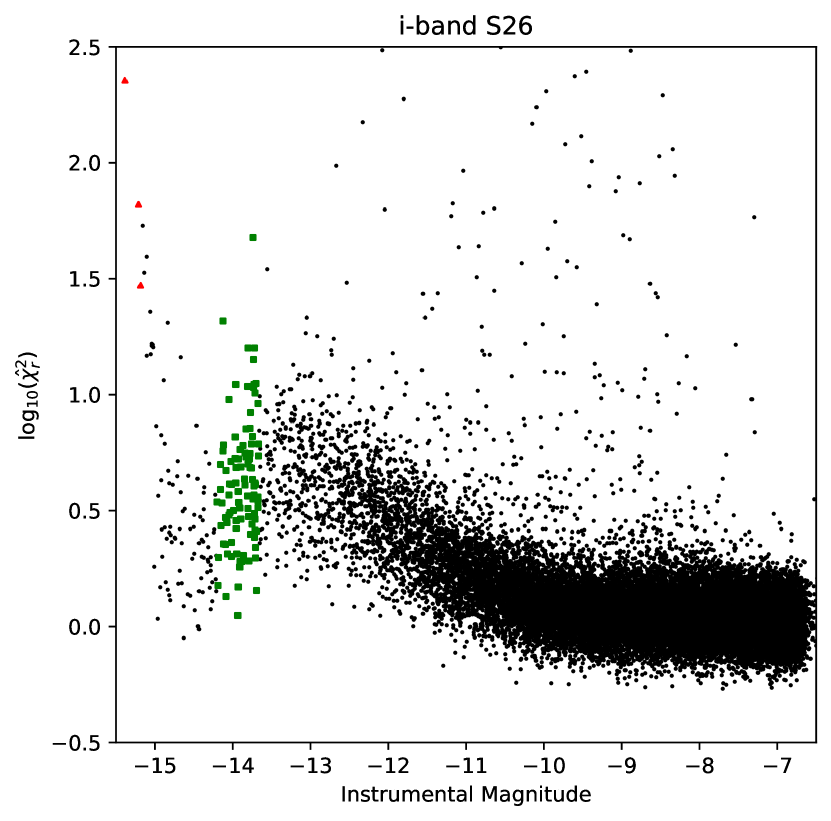
Figure 30: Scatter plot of sources not flagged by the CP as saturated when the saturation threshold was set too low. The plot shows the $\hat{\chi}^{2}_{r}$ as a function of the estimated source flux (in instrumental magnitudes). There is a sharp linear increase in the $\log_{10}(\hat{\chi}^{2}_{r})$ at the brightest magnitudes ($<-15$), indicative of sources at/near saturation being poorly modeled by the average PSF. The three brightest unflagged sources are shown as red triangles and a set of 100 bright, but unsaturated reference sources are shown as green squares. This example is for an $i$-band image taken by CCD S26.

Appendix C Computational Details

The overwhelming majority of computational time was spent using crowdsource and CloudCovErr.jl in processing individual exposures. These runs were executed on the FASRC Cannon cluster at Harvard University on compute nodes with water-cooled Intel 24-core Platinum 8268 Cascade Lake CPUs with 192GB RAM and dual AVX-512 fused multiply-add (FMA) units running 64-bit CentOS 7. We used GNU Parallel (Tange, 2021) to spawn, manage restarts, and track the computational time of processing the 21,430 exposures (each containing 60-61 CCDs of $2046\times 4094$ pixels) across many multi-cpu SLURM batch allocations.

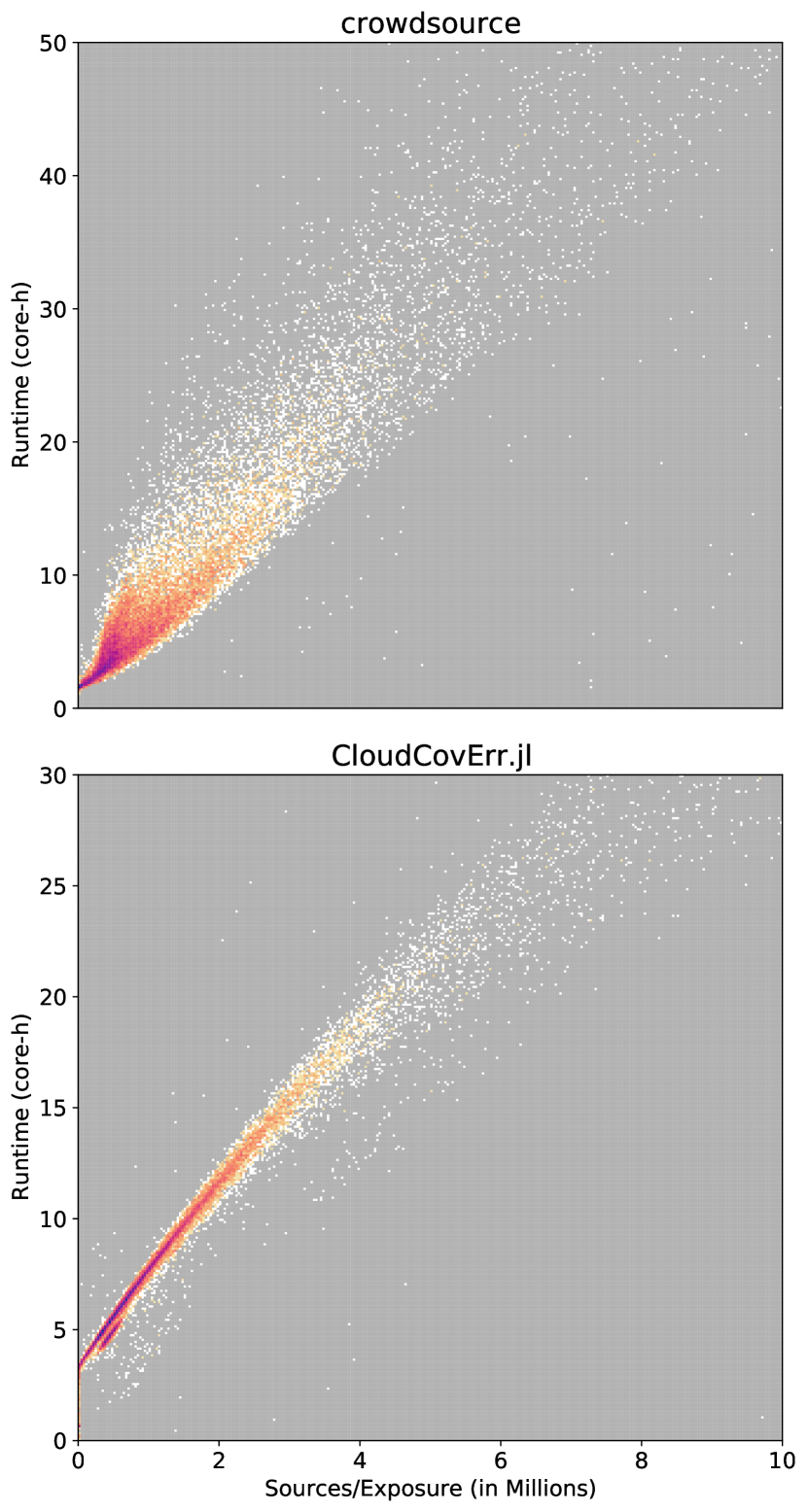
Figure 31: Histogram showing the runtime of an exposure versus the number of sources found in that exposure for crowdsource (top) and CloudCovErr.jl (bottom) processing of DECaPS2. The color scale is in log-density, and each panel has its own normalization (light, white, low; dark, blue, high density).

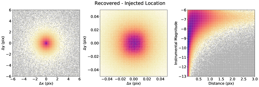
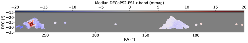
Figure 32: (Left): Histogram (2D) of the position errors for recovering injected sources. Color scale shows log density (light, white, low; dark, blue, high). (Center): Same as (Left), but with linear density and focused on the central peak. (Right): Histogram (2D) of the distance error between the recovered and injected source locations as a function of the brightness of the injected source. Color scale shows log density (light, white, low; dark, blue, high).

Figure 33: Median offset between DECaPS2-PS1 in $r$-band for stars between between $15-17$th mag, as defined using the color transform between the PS1 and DECaPS filter systems which was derived using the calibration field at $({\rm RA,DEC})=(100\degree,-27\degree)$.

For the crowdsource runs, a first pass limiting memory to 3.8 G/exposure succeeded on $\sim 80\%$ of the survey footprint. The remaining exposures, which represent fields with high stellar densities, were rerun with 9.8 GB of memory. The total crowdsource runtime was 230k core-hours. The CloudCovErr.jl runs used $3.6-4.8$ GB per exposure (median 3.7 GB) and completed in 203k core-hours (see Saydjari & Finkbeiner (2022) for more details). The runtimes demonstrate high linearity with respect to the number of stars per exposure (Figure 31). Building images for the Legacy Survey Viewer using legacypipe took $\sim 2.4$k core-h each for the images and model images, with $95\%$ of the run completing with 7.7 GB of RAM (the rest completing with a 35 GB/core allocation). Processing the raw images by the DECam Community Pipeline was largely I/O bound.

A bug in the crowdsource injection module was found after the run, which impacts the “true” source locations saved in the MCK extension of the crowdsource injection catalogs. The pixelization of the PSF and the integer location for its injection into the image was rounded in one place and truncated in another. Thus, the “true” injected source coordinate is -1 pixel from the reported coordinate in the injection catalog for sources with positions mod 1 $>0.5$. An example of how to convert the injection catalog to the true positions is provided in Section 9.

Appendix D Location Precision

We use the injection tests described in Section 7 to evaluate the precision with which crowdsource can recover source locations, focusing on the unblended limit. Figure 33 shows histograms of the difference between the recovered and injected locations of the synthetic sources added to the image. We restrict to unblended sources by requiring fracflux $>0.75$, that no source in the original image within 2 FWHM of the injected location, that the recovered source location is not pulled toward the nearest neighboring source by more than 1 pixel, and that the source/background flux be positive.

The left panel shows the logarithmic density over a larger range and exhibits rotational symmetry. The median offset in both x and y are $<1\times 10^{-3}$ pixels, illustrating the accuracy of the recovered source locations from crowdsource. The middle panel focuses on the central peak with a linear density scale, indicating slight distortions from full rotational symmetry. The right panel shows a logarithmic histogram of the recovered-injected distance as a function of the injected source magnitude. The astrometric precision is clearly a function of the source flux, decreasing for fainter sources. Characterizing the faint astrometry would require a more careful consideration of the cuts used to exclude blended or misidentified sources.

To compare to Figure 12, we report the median recovered-injected distance for bright injected sources (brighter than $\sim 19$th $g$-band mag, $-11$ instrumental mag) which is 0.016 pixels, or 4 mas given the DECam pixel scale. This would be the astrometric performance if sources had exactly the crowdsource PSF model and the WCS solution across the CCD were perfect. In DECaPS2, the WCS solution used is that from the CP, without any modification. Even over the portion of the DECaPS2 footprint with WCS solutions from Gaia eDR3, the typical median astrometric errors per NSide=512 HEALPix pixel were 17.5 mas. This suggests that crowdsource is not the limiting factor on astrometry and improvements on astrometry beyond 17.5 mas will require careful treatment of higher-order terms in the WCS, including effects such as those considered by Bernstein et al. (2017) and Fortino et al. (2021).

Appendix E PS1 Color Transform Variation

The DECaPS2 absolute calibration is tied to PS1 via a color transform described in Section 6.2. The color transformation was derived on a low-reddening field so that it could capture the effects of varying stellar temperature without confusion caused by the effect of varying reddening.

While the color transformation used explicitly does not account for how dust affects colors, we can nevertheless apply it even in highly extinguished areas to measure how PS1 and DECam colors compare across the survey footprint. Figure 33 shows this comparison for $r$-band, restricting to stars measured in PS1 $g,r,i$-band, DECaPS $r$-band, and between $15-17$th mag in $r$-band. The crossmatch requires sources in PS1 to be within 0.5” of the source location in DECaPS2 and that there be no more than one match for a given source.

In the outer Galaxy, small offsets in DECaPS2-PS1 of $<5$ mmag are observed. In the inner Galaxy, outside of highly extinguished regions in the Pipe Nebula, typical offsets are negative and $<15$ mmag. Over the entire overlap, the standard deviation of the offsets, excluding regions of high extinction around the Pipe Nebula, is 3.7 mmag. We consider this to be excellent agreement between two different surveys performed by different systems and tied together only by a single field. A few regions with offsets of $\sim 50$ mmag are are observed in regions of high extinction, reflecting our color transformation’s neglect for the effect of extinction.

Another DECam program, the Blanco DECam Bulge Survey (BDBS), suggested that DECaPS was inconsistent with PS1 by 200 mmag on several bulge fields and in several filters, including r-band (Johnson et al., 2020). However, this large offset was due to the combination of not applying a color transformation and performing the comparison in regions of large reddening. Accounting for these two effects resolves the apparent discrepancy .

Appendix F Detection Threshold Bias

We derive the photometric bias due to the presence of a detection threshold as a function of the true SNR of the source. Then, we apply an approximation to obtain a functional form which can be fit to the faint-limit bias in synthetic injection tests. The single free parameter in this fit is exactly the detection limit in SNR of the photometric pipeline.

Suppose we are considering an isolated source (star) with true flux $gf_{0}$ on a constant background with flux $gb_{0}$, where $g$ is the detector gain so that we convert to and work entirely in photoelectrons. The point spread function (PSF) of the source through the imaging system is $p(x,y)$, which has an effective area $A_{\rm{eff}}=\frac{\int p}{\int p^{2}}=\frac{1}{\int p^{2}}$.

We work in the faint limit where the measurement noise is dominated by the Poisson statistics of the background counts. We will further work in the large count limit of all Poisson distributions so that we can take the Gaussian approximation. In this limit, we can define the SNR of the (true) source $s_{0}$ and the flux of a source just at the detection threshold ($f_{d}$) imposed by a detection limit $s_{d}$ on (observed) SNR.

$$s_{0}=\frac{gf_{0}}{\sqrt{A_{\rm{eff}}gb_{0}}}=\frac{gf_{0}}{\sigma}\quad\text{and}\quad s_{d}=\frac{gf_{d}}{\sqrt{A_{\rm{eff}}gb_{0}}}=\frac{gf_{d}}{\sigma}$$ (F1)

In addition to $s_{0}$ and $s_{d}$ considered here, both the apparent SNR given the recovered flux $s_{r}$ and the SNR of the injected source accounting for the realization of the Poisson noise $s_{i}$ are distinct quantities important for future analyses.

To measure the bias, we compute the expectation value of $y=gf-gf_{0}+\epsilon$, where $f$ is a draw of the source flux and $\epsilon$ is a draw of the background-induced noise on the PSF photometry. In the background-dominated noise limit, $y\sim\mathcal{N}(\mu=0,\,\sigma^{2}=A_{\rm{eff}}gb_{0})$. However, we only detect a source when the estimated flux has sufficient SNR, or as a flux condition, when $gf+\epsilon>gf_{d}$. Thus, we take the expectation value only over values of $y$ above threshold.

$$\left<gf-gf_{0}\right>=\frac{\int_{f_{d}-f_{0}}^{\infty}dy\,h(y)y}{\int_{f_{d}-f_{0}}^{\infty}dy\,h(y)}\quad\text{where}\quad h(y)=\frac{1}{\sqrt{2\pi}\sigma}e^{-\frac{1}{2}\left(\frac{y-\mu}{\sigma}\right)^{2}}$$ (F2)

is the usual Gaussian PDF given $y\sim\mathcal{N}(\mu=0,\,\sigma^{2}=A_{\rm{eff}}gb_{0})$. These are just improper Gaussian integrals and, normalizing by $gf_{0}$ so we can talk about fractional errors, we obtain

$$\frac{\left<gf-gf_{0}\right>}{gf_{0}}=\sqrt{\frac{2}{\pi}}\frac{\sigma}{gf_{0}}\frac{e^{-x^{2}}}{\operatorname{erfc}(x)}\quad\text{where}\quad x=\frac{gf_{d}-gf_{0}}{\sqrt{2}\sigma}$$ (F3)

and $\operatorname{erfc}$ is the complementary error function.

Using Equation F1, we can transform this result to be only in terms of the true SNR of the source $s_{0}$ and the detection threshold SNR $s_{d}$. Then it is clear that all factors of the gain, effective area of the PSF, and the background level drop out.

$$\frac{\left<f-f_{0}\right>}{f_{0}}=\sqrt{\frac{2}{\pi}}\frac{1}{s_{0}}\frac{e^{-x^{2}}}{\operatorname{erfc}(x)}\quad\text{where}\quad x=\frac{s_{d}-s_{0}}{\sqrt{2}}$$ (F4)

Under the limits taken, this result is exact, but difficult to work with given that $\operatorname{erfc}$ is not an elementary function. Since we are interested in the faint limit where the sources are near threshold ($x=f_{d}-f_{0}\approx 0$), we use the approximation for $\operatorname{erfc}$ due to Karagiannidis & Lioumpas (2007), often called the KL approximation.

$$\operatorname{erfc}(x)\approx\frac{\left(1-e^{-Ax}\right)e^{-x^{2}}}{B\sqrt{\pi}x}\quad\text{where}\quad(A,B)=(1.98,1.135)$$ (F5)

Substituting into Equation F4, we obtain a functional form for the threshold-induced bias with a single free parameter that can be easily fit to data from synthetic injection tests. That single free parameter $s_{d}$ is the effective detection threshold of the photometric pipeline which can differ from the targeted threshold and is not known a priori. Given that the KL approximation is best for $x>0$ and $\operatorname{erfc}(-x)=2-\operatorname{erfc}(x)$, one could define Equation F5 piecewise for higher accuracy. Further, one could simply evaluate $\operatorname{erfc}$ at every point and use the exact form (Equation F4) for the fit. However, the KL approximation, which overestimates the bias at $x<0$ ($s_{0}>s_{d}$) is a slightly better fit (by approximately a factor of 2 in the residuals) to the data than the true functional form using Equation F4). We expect this is the result of unmodeled biases, such as in the selection we apply to the injection tests, which will be the focus of future work.

$$\frac{\left<f-f_{0}\right>}{f_{0}}=\frac{B\left(\frac{s_{d}}{s_{0}}-1\right)}{1-e^{-\frac{A}{\sqrt{2}}\left(s_{d}-s_{0}\right)}}\quad\text{where}\quad(A,B)=(1.98,1.135)$$ (F6)

At exactly $s=s_{0}$, Equation F6 has a removable singularity and we find

$$\frac{\left<f-f_{0}\right>}{f_{0}}\Bigr{|}_{s_{0}=s_{d}}=\frac{B\sqrt{2}}{As_{d}}\quad\text{where}\quad(A,B)=(1.98,1.135)$$ (F7)

The case where $s_{0}=s$ is exactly when $f_{0}=f_{d}$, when the threshold falls in the middle of the Gaussian PDF for the observed flux distribution. That is when a source will be detected exactly 50% of the time as a result of the detection threshold. Since the source flux where that occurs is usually taken to be the definition of the depth, we can interpret $f_{d}$ as the photometric depth. In fact, many photometric surveys estimate imaging depth by assuming a photometric pipeline can retrieve $s_{d}$-sigma (generally 5-6) sources and then using Equation F1 to solve for the flux limit given the (average) PSF and (average) background counts of the image. However, this measure of depth is limited by that averaging as well as accurately knowing $s_{d}$.

Instead, using injection tests, we can empirically measure the real $s_{d}$ achieved by a given pipeline by fitting the faint-limit bias and then use the predicted fractional error at $s_{d}$ to determine the depth by the flux at which such a bias is observed. In the case of an ideal isolated source with perfect PSF modeling and a constant background, the definition of photometric depth via bias in synthetic injections is identical to the usual definition.

In the crowded limit, it is not exactly clear how to extend the usual definition of depth. How do we measure when 50% of injected sources at a given flux are recovered? In the crowded limit, there will often be a detection within a small radius around the injected source location. That detection could be a source that is a “good” model of the injected source, a model that combines the flux of the injected source with a neighboring (pre-existing) source, or a detection of a completely different neighboring source and the injected source was simply not detected. One must then make a quality cut on the recovered detections, such as a maximum fractional flux error, to restrict to detections that are “good” models of the injected source. However, in the highly crowded limit, the percentage of injected sources that have a high-quality detection might be small and the choice of quality cuts effectively arbitrary, though those choices have a large impact on the reported depth.

The faint-limit bias approach to measuring photometric depth proposed here does not suffer from these problems. In the crowded limit, where all injected sources may end up absorbing flux from pre-existing sources, this definition very cleanly extends to give the magnitude such that the flux estimates of sources are as biased as they would be by the detection threshold alone in an isolated field. This retains the key notion of photometric depth as an indicator of the faintest reliable star in the catalog.

In the $s_{0}<<s_{d}$ limit (source fainter than threshold) of Equation F6, the bias diverges positively. In the limit $s_{0}>>s_{d}$ (source brighter than threshold), the bias becomes exponentially small as a function of $s_{0}$. This rapid falloff means the detection threshold bias is only important for sources near the threshold. However, the other faint-limit bias discussed in the main text, which results from using the maximum likelihood position, approaches zero fractional bias much more slowly as a function of $s_{0}$. As such, when fitting the faint-limit bias, we find it necessary to model both sources of bias. We will make the naive assumption that the two biases are independent and simply sum them. Taking the highest-order form in Portillo et al. (2020), we obtain the combined functional form that we actually fit

$$\boxed{\frac{\left<f-f_{0}\right>}{f_{0}}=\frac{B\left(\frac{s_{d}}{s_{0}}-1\right)}{1-e^{-\frac{A}{\sqrt{2}}\left(s_{d}-s_{0}\right)}}+\frac{1}{s_{0}^{2}}+\frac{1}{s_{0}^{4}}\quad\text{where}\quad(A,B)=(1.98,1.135)}$$ (F8)

and define the photometric depth as the flux such that the fractional bias is

$$\boxed{\frac{\left<f-f_{0}\right>}{f_{0}}\Bigr{|}_{s_{0}=s_{d}}=\frac{B\sqrt{2}}{As_{d}}+\frac{1}{s_{d}^{2}}+\frac{1}{s_{d}^{4}}\quad\text{where}\quad(A,B)=(1.98,1.135).}$$ (F9)

As mentioned in the text, we do not apply a “correction” for this bias to the DECaPS2 catalog. The main requirement for such a correction is the need to use a prior on the distribution of true source fluxes (even several $\sigma$ below the detection threshold) so that one can convert the bias on true SNR to a bias on observed SNR. In addition, there is a bias-variance trade-off in applying such a correction (as in Portillo et al. 2020) which would need to be computed. However, near the detection limit, the selection of only sources above the threshold subsamples the usual Poisson distribution and can impact the scatter of the source distribution. Finally, especially in the crowded limit, not detecting a source can bias neighboring sources and a low SNR bias correction should depend on the source density as well.

References

- Wei (2001) 2001, The Astrophysical Journal, Volume 548, Issue 1, pp. 296-309., 548, 296, doi: 10.1086/318651
- Abbott et al. (2021) Abbott, T. M. C., Adamów, M., Aguena, M., et al. 2021, ApJS, 255, 20, doi: 10.3847/1538-4365/ac00b3
- Aihara et al. (2018) Aihara, H., Arimoto, N., Armstrong, R., et al. 2018, PASJ, 70, S4, doi: 10.1093/pasj/psx066
- Akeson et al. (2019) Akeson, R., Armus, L., Bachelet, E., et al. 2019, arXiv e-prints, arXiv:1902.05569. https://arxiv.org/abs/1902.05569
- Alonso-García et al. (2018) Alonso-García, J., Saito, R. K., Hempel, M., et al. 2018, A&A, 619, A4, doi: 10.1051/0004-6361/201833432
- Antilogus et al. (2014) Antilogus, P., Astier, P., Doherty, P., Guyonnet, A., & Regnault, N. 2014, Journal of Instrumentation, 9, C03048, doi: 10.1088/1748-0221/9/03/C03048
- Astropy Collaboration et al. (2013) Astropy Collaboration, Robitaille, T. P., Tollerud, E. J., et al. 2013, A&A, 558, A33, doi: 10.1051/0004-6361/201322068
- Benjamin et al. (2003) Benjamin, R. A., Churchwell, E., Babler, B. L., et al. 2003, PASP, 115, 953, doi: 10.1086/376696
- Bernstein et al. (2017) Bernstein, G. M., Armstrong, R., Plazas, A. A., et al. 2017, PASP, 129, 074503, doi: 10.1088/1538-3873/aa6c55
- Bertin & Arnouts (1996) Bertin, E., & Arnouts, S. 1996, A&AS, 117, 393, doi: 10.1051/aas:1996164
- Bohlin (2014) Bohlin, R. C. 2014, AJ, 147, 127, doi: 10.1088/0004-6256/147/6/127
- Bosch et al. (2018) Bosch, J., Armstrong, R., Bickerton, S., et al. 2018, PASJ, 70, S5, doi: 10.1093/pasj/psx080
- Brewer et al. (2013) Brewer, B. J., Foreman-Mackey, D., & Hogg, D. W. 2013, AJ, 146, 7, doi: 10.1088/0004-6256/146/1/7
- Burleigh et al. (2020) Burleigh, K. J., Landriau, M., Dey, A., et al. 2020, arXiv e-prints, arXiv:2002.05828. https://arxiv.org/abs/2002.05828
- Cardelli et al. (1989) Cardelli, J. A., Clayton, G. C., & Mathis, J. S. 1989, ApJ, 345, 245, doi: 10.1086/167900
- Chambers et al. (2016) Chambers, K. C., Magnier, E. A., Metcalfe, N., et al. 2016, arXiv e-prints, arXiv:1612.05560. https://arxiv.org/abs/1612.05560
- Churchwell et al. (2009) Churchwell, E., Babler, B. L., Meade, M. R., et al. 2009, PASP, 121, 213, doi: 10.1086/597811
- Dey et al. (2019) Dey, A., Schlegel, D. J., Lang, D., et al. 2019, AJ, 157, 168, doi: 10.3847/1538-3881/ab089d
- Draine (2003) Draine, B. T. 2003, ARA&A, 41, 241, doi: 10.1146/annurev.astro.41.011802.094840
- Everett et al. (2022) Everett, S., Yanny, B., Kuropatkin, N., et al. 2022, ApJS, 258, 15, doi: 10.3847/1538-4365/ac26c1
- Feder et al. (2020) Feder, R. M., Portillo, S. K. N., Daylan, T., & Finkbeiner, D. 2020, AJ, 159, 163, doi: 10.3847/1538-3881/ab74cf
- Flaugher et al. (2015) Flaugher, B., Diehl, H. T., Honscheid, K., et al. 2015, AJ, 150, 150, doi: 10.1088/0004-6256/150/5/150
- Fortino et al. (2021) Fortino, W. F., Bernstein, G. M., Bernardinelli, P. H., et al. 2021, AJ, 162, 106, doi: 10.3847/1538-3881/ac0722
- Gorbikov et al. (2010) Gorbikov, E., Brosch, N., & Afonso, C. 2010, Ap&SS, 326, 203, doi: 10.1007/s10509-009-0242-0
- Górski et al. (2005) Górski, K. M., Hivon, E., Banday, A. J., et al. 2005, ApJ, 622, 759, doi: 10.1086/427976
- Green et al. (2019) Green, G. M., Schlafly, E., Zucker, C., Speagle, J. S., & Finkbeiner, D. 2019, ApJ, 887, 93, doi: 10.3847/1538-4357/ab5362
- Harris (1996) Harris, W. E. 1996, AJ, 112, 1487, doi: 10.1086/118116
- Huang et al. (2018) Huang, S., Leauthaud, A., Murata, R., et al. 2018, PASJ, 70, S6, doi: 10.1093/pasj/psx126
- Hunter (2007) Hunter, J. D. 2007, Computing in Science and Engineering, 9, 90, doi: 10.1109/MCSE.2007.55
- Johnson et al. (2020) Johnson, C. I., Rich, R. M., Young, M. D., et al. 2020, MNRAS, 499, 2357, doi: 10.1093/mnras/staa2393
- Jones et al. (2020) Jones, R. L., Bannister, M. T., Bolin, B. T., et al. 2020, arXiv preprint arXiv:2009.07653
- Karagiannidis & Lioumpas (2007) Karagiannidis, G. K., & Lioumpas, A. S. 2007, IEEE Communications Letters, 11, 644
- Kong et al. (2020) Kong, H., Burleigh, K. J., Ross, A., et al. 2020, MNRAS, 499, 3943, doi: 10.1093/mnras/staa2742
- Lang et al. (2016) Lang, D., Hogg, D. W., & Mykytyn, D. 2016, The Tractor: Probabilistic astronomical source detection and measurement. http://ascl.net/1604.008
- Lawrence et al. (2007) Lawrence, A., Warren, S. J., Almaini, O., et al. 2007, MNRAS, 379, 1599, doi: 10.1111/j.1365-2966.2007.12040.x
- Liu et al. (2021) Liu, R., McAuliffe, J. D., & Regier, J. 2021, arXiv e-prints, arXiv:2102.02409. https://arxiv.org/abs/2102.02409
- Lucas et al. (2008) Lucas, P. W., Hoare, M. G., Longmore, A., et al. 2008, MNRAS, 391, 136, doi: 10.1111/j.1365-2966.2008.13924.x
- Magnier et al. (2013) Magnier, E. A., Schlafly, E., Finkbeiner, D., et al. 2013, ApJS, 205, 20, doi: 10.1088/0067-0049/205/2/20
- Magnier et al. (2020) Magnier, E. A., Sweeney, W. E., Chambers, K. C., et al. 2020, ApJS, 251, 5, doi: 10.3847/1538-4365/abb82c
- Minniti et al. (2010) Minniti, D., Lucas, P. W., Emerson, J. P., et al. 2010, New A, 15, 433, doi: 10.1016/j.newast.2009.12.002
- Nidever et al. (2021) Nidever, D. L., Dey, A., Fasbender, K., et al. 2021, AJ, 161, 192, doi: 10.3847/1538-3881/abd6e1
- Padmanabhan et al. (2008) Padmanabhan, N., Schlegel, D. J., Finkbeiner, D. P., et al. 2008, ApJ, 674, 1217, doi: 10.1086/524677
- Perez & Granger (2007) Perez, F., & Granger, B. E. 2007, Computing in Science and Engineering, 9, 21, doi: 10.1109/MCSE.2007.53
- Portillo et al. (2017) Portillo, S. K. N., Lee, B. C. G., Daylan, T., & Finkbeiner, D. P. 2017, AJ, 154, 132, doi: 10.3847/1538-3881/aa8565
- Portillo et al. (2020) Portillo, S. K. N., Speagle, J. S., & Finkbeiner, D. P. 2020, AJ, 159, 165, doi: 10.3847/1538-3881/ab76ba
- Saito et al. (2012) Saito, R. K., Hempel, M., Minniti, D., et al. 2012, A&A, 537, A107, doi: 10.1051/0004-6361/201118407
- Saydjari & Finkbeiner (2022) Saydjari, A. K., & Finkbeiner, D. P. 2022, arXiv e-prints, arXiv:2201.07246. https://arxiv.org/abs/2201.07246
- Saydjari & Schlafly (2022, in prep.) Saydjari, A. K., & Schlafly, E. F. 2022, in prep.
- Schlafly (2021) Schlafly, E. F. 2021, crowdsource: Crowded field photometry pipeline, Astrophysics Source Code Library, record ascl:2106.004. http://ascl.net/2106.004
- Schlafly et al. (2019) Schlafly, E. F., Meisner, A. M., & Green, G. M. 2019, ApJS, 240, 30, doi: 10.3847/1538-4365/aafbea
- Schlafly et al. (2017) Schlafly, E. F., Peek, J. E. G., Finkbeiner, D. P., & Green, G. M. 2017, ApJ, 838, 36, doi: 10.3847/1538-4357/aa619d
- Schlafly et al. (2012) Schlafly, E. F., Finkbeiner, D. P., Jurić, M., et al. 2012, ApJ, 756, 158, doi: 10.1088/0004-637X/756/2/158
- Schlafly et al. (2016) Schlafly, E. F., Meisner, A. M., Stutz, A. M., et al. 2016, ApJ, 821, 78, doi: 10.3847/0004-637X/821/2/78
- Schlafly et al. (2018) Schlafly, E. F., Green, G. M., Lang, D., et al. 2018, ApJS, 234, 39, doi: 10.3847/1538-4365/aaa3e2
- Scholz et al. (2015) Scholz, R. D., Kharchenko, N. V., Piskunov, A. E., Röser, S., & Schilbach, E. 2015, A&A, 581, A39, doi: 10.1051/0004-6361/201526312
- Skrutskie et al. (2006) Skrutskie, M. F., Cutri, R. M., Stiening, R., et al. 2006, AJ, 131, 1163, doi: 10.1086/498708
- Stetson (1987) Stetson, P. B. 1987, PASP, 99, 191, doi: 10.1086/131977
- Stubbs & Tonry (2006) Stubbs, C. W., & Tonry, J. L. 2006, ApJ, 646, 1436, doi: 10.1086/505138
- Tange (2021) Tange, O. 2021, GNU Parallel 20210622 (’Protasevich’), Zenodo, doi: 10.5281/zenodo.5013933
- The Dark Energy Survey Collaboration (2005) The Dark Energy Survey Collaboration. 2005, arXiv e-prints, astro. https://arxiv.org/abs/astro-ph/0510346
- Valdes et al. (2014) Valdes, F., Gruendl, R., & DES Project. 2014, in Astronomical Society of the Pacific Conference Series, Vol. 485, Astronomical Data Analysis Software and Systems XXIII, ed. N. Manset & P. Forshay, 379
- van der Walt et al. (2011) van der Walt, S., Colbert, S. C., & Varoquaux, G. 2011, Computing in Science and Engineering, 13, 22, doi: 10.1109/MCSE.2011.37
- Wright et al. (2010) Wright, E. L., Eisenhardt, P. R. M., Mainzer, A. K., et al. 2010, AJ, 140, 1868, doi: 10.1088/0004-6256/140/6/1868
- Zelko & Finkbeiner (2020) Zelko, I. A., & Finkbeiner, D. P. 2020, The Astrophysical Journal, 904, 38, doi: 10.3847/1538-4357/abbb8d