Formalizing the Problem of Side Effect Regularization

Abstract

AI objectives are often hard to specify properly. Some approaches tackle this problem by regularizing the ai’s side effects: Agents must weigh off “how much of a mess they make” with an imperfectly specified proxy objective. We propose a formal criterion for side effect regularization via the assistance game framework (Shah et al., 2021). In these games, the agent solves a partially observable Markov decision process (pomdp) representing its uncertainty about the objective function it should optimize. We consider the setting where the true objective is revealed to the agent at a later time step. We show that this pomdp is solved by trading off the proxy reward with the agent’s ability to achieve a range of future tasks. We empirically demonstrate the reasonableness of our problem formalization via ground-truth evaluation in two gridworld environments.

1 Introduction

We need to build aligned ai systems, not just capable ai systems. For example, recommender systems which maximize app usage might provoke addiction in their users. Users need the ai system’s behavior to be aligned with their interests.

When optimizing a formally specified objective, agents often have unforeseen negative side effects. An agent rewarded for crossing a room may break furniture in order to cross the room as quickly as possible. This simple reward function neglects our complex preferences about the rest of the environment. One way to define a negative side effect is that it reduces the potential value for the (unknown) true reward function.

Intuitively, we want the agent to optimize the specified reward function, while also preserving its ability to pursue other goals in the environment. Existing approaches seem promising, but there is no consensus on the formal optimization problem which is being solved by side effect regularization approaches.

We formalize the optimization problem as a special kind of assistance game (Shah et al., 2021), played by the ai (the assistant $\mathbf{A}$) and its designer (the human $\mathbf{H}$). An assistance game is a pomdp with common knowledge of prior uncertainty about the reward function. The human observes the true reward function, but the assistant does not. In our formulation, we assume full observability, and that the human’s actions are communicative—they do not affect transitions and do not depend on the current observation. We also suppose that the human reveals the true reward function after some amount of time, but $\mathbf{A}$ otherwise has no way of learning more about the true reward function.

This delayed specification assistance game formalizes a range of natural use cases beyond side effect minimization. For example, when not assigned a customer, an Uber driver may navigate to a state which allows them to quickly pick up a range of probable customers—with the assigned route being the driver’s initially unknown true objective. Alternatively, consider an empty restaurant which expects a range of probable customers. When a customer arrives and makes an order, they communicate the restaurant’s initially unknown food preparation objective. Therefore, the restaurant should prepare to satisfy a range of objectives at the expected customer arrival times.

Contributions.

We formalize delayed specification assistance games. We show that solving this game reduces to a trade-off between prior-expected reward and preservation of the agent’s future ability to achieve a range of plausible objectives (Section 2.2). We also show that when the human has a fixed per-timestep probability of communicating the true reward function, the resultant pomdp is solved by optimizing a Markovian state-based reward function trading off immediate expected reward with ability achieve a range of future objectives (Section 2.2). We consider the side-effect regularization problem in our new formal framework. We experimentally illustrate the reasonableness of this framework in two ai safety gridworlds (Leike et al., 2017).

2 Delayed specification assistance games

We formalize a special kind of partially observable Markov decision process (pomdp), which we then show is solved by an objective which trades off expected true reward with the ability to optimize a range of possible true reward functions. We show several theoretical results on the hardness and form of solutions to this pomdp. In section 3, we will apply this framework to analyze side effect regularization situations.

2.1 Assistance game formalization

This game is played by two agents, the human $\mathbf{H}$ and the assistant $\mathbf{A}$. The environment is fully observable because both agents observe the world state $s\in\mathcal{S}$ at each time step, but the true reward function $R_{\theta}$ is hidden to $\mathbf{A}$. Both agents may select history-dependent policies, but only the human can condition their policy on $R_{\theta}$.

Following Shah et al. (2021), a communicative fully-observable assistance game $\mathcal{M}$ is a tuple $\langle\mathcal{S},\left\{\mathcal{A}^{\mathbf{H}},\mathcal{A}^{\mathbf{A}}\right\},T,s_{0},\gamma,\langle\Theta,R_{\theta},\mathcal{D}\rangle\rangle$, where we take $\mathcal{S}$ to be a finite state space, $\mathcal{A}^{\mathbf{H}}$ to be the human action space, and $\mathcal{A}^{\mathbf{A}}$ to be the finite agent action space. $T:\mathcal{S}\times\mathcal{A}^{\mathbf{H}}\times\mathcal{A}^{\mathbf{A}}\to\Delta(\mathcal{S})$ is the (potentially stochastic) transition function (where $\Delta(X)$ is the set of probability distributions over set $X$), $s_{0}$ is the initial state, and $\gamma\in(0,1)$ is the discount factor. We assume that the game is communicative, which means that the human action choice does not affect the transitions.

$\Theta$ is the set of potential reward function parameters $\theta$, which induce reward functions $R_{\theta}:\mathcal{S}\to\mathbb{R}$. $\mathcal{D}$ is a probability distribution over $\Theta$. In this work, we let $\Theta\coloneqq\mathbb{R}^{\mathcal{S}}$ (the set of all state-based reward functions), and so each $R_{\theta}:s\mapsto\theta(s)$. We differ from Shah et al. (2021) in assuming that the reward is only a function of the current state.

In a delayed specification assistance game, we assume that the agent will know the true reward function $R_{\theta}$ after some time $t$. We have uncertainty $\mathcal{D}$ about the true reward function we want to specify. The agent has no way of learning more about $R_{\theta}$ before time $t$.

The human policy $\pi^{\mathbf{H}}:\Theta\times\mathcal{S}\mapsto\mathcal{A}^{\mathbf{H}}$ is a goal-conditioned policy. Both agents can observe the state, but only the human can observe the unknown reward parameterization $\theta\in\Theta$. Our simplified model of the problem assumes that the human action space $\mathcal{A}^{\mathbf{H}}=\mathbb{R}^{\mathcal{S}}\cup\{a_{\text{no-op}}^{\mathbf{H}}\}$: the human can communicate all their hidden information, a real-valued state-based reward function, in a single turn or they do nothing. We suppose that the human communicates the complete reward information $R_{\theta}\in\mathbb{R}^{\mathcal{S}}$ at some random time step $t\sim\mathcal{T}$, which is independent of the state-action history:

$$\pi^{\mathbf{H}}(s_{0}a^{\mathbf{A}}_{0}a^{\mathbf{H}}_{0}\cdots s_{t}a^{\mathbf{A}}_{t},R_{\theta})\coloneqq\begin{cases}R_{\theta}&\text{with probability }\operatorname*{\mathbb{P}}\left(\mathcal{T}=t\right)\\ a_{\text{no-op}}^{\mathbf{H}}&\text{else.}\end{cases}$$ (1)

While the human policy assumption is simplistic, it does capture many real world scenarios with unknown reward functions and the analysis which follows is still interesting.

[Solutions to the assistance game (Shah et al., 2021)]definitiongamesoln An assistant policy $\pi^{\mathbf{A}}$ induces a probability distribution over trajectories: $\tau\sim\left\langle s_{0},\theta,\pi^{\mathbf{H}},\pi^{\mathbf{A}}\right\rangle,\tau\in\left[S\times A^{\mathbf{H}}\times A^{\mathbf{A}}\right]^{*}$. The expected reward of $\pi^{\mathbf{A}}$ for $\left\langle\mathcal{M},\pi^{\mathbf{H}}\right\rangle$ is

$$\mathrm{ER}\left(\pi^{\mathbf{A}}\right)=\underset{\theta\sim\mathcal{D},\tau\sim\left\langle s_{0},\theta,\pi^{\mathbf{H}},\pi^{\mathbf{A}}\right\rangle}{\mathbb{E}}\left[\sum_{i=0}^{\infty}\gamma^{i}R_{\theta}\left(s_{i},a_{i}^{\mathbf{H}},a_{i}^{\mathbf{A}},s_{i+1}\right)\right].$$

A solution of $\left\langle\mathcal{M},\pi^{\mathbf{H}}\right\rangle$ maximizes expected reward: $\pi^{\mathbf{A}}\in\underset{\tilde{\pi}^{\mathbf{A}}}{\operatorname{argmax}}\,\mathrm{ER}\left(\tilde{\pi}^{\mathbf{A}}\right)$.

Once the assistant has observed $R_{\theta}$, section 2.1 shows that it should execute an optimal policy $\pi\in\Pi^{*}\left(R_{\theta},\gamma\right)$ thereafter.

[Optimal policy set function (Turner et al., 2021)]definitionFORMdefOptPi $\Pi^{*}\left(R,\gamma\right)$ is the optimal policy set for reward function $R$ at discount rate $\gamma\in(0,1)$.

[Follow an optimal policy after observing $R_{\theta}$]lemoptPolSoln If there is a solution to the pomdp, then there exists a solution $\pi^{\mathbf{A}}_{\text{switch}}$ which, after observing human action $R_{\theta}$ at any point in its history, follows $\pi^{*}_{R_{\theta}}\in\Pi^{*}\left(R_{\theta},\gamma\right)$ thereafter.

Proof.

By eq. 1, $\pi^{\mathbf{H}}$ outputs reward function $R_{\theta}$ only if $R_{\theta}$ is the true reward function. By the definition of $\Pi^{*}\left(R_{\theta},\gamma\right)$, following an optimal policy maximizes expected return for $R_{\theta}$. ∎

[Prefix policies]definitionprefixPol Let $\pi^{\mathbf{A}}$ be a assistant policy. Its prefix policy $\pi$ is the restriction of $\pi^{\mathbf{A}}$ to histories in which the human has only taken the action $a_{\text{no-op}}^{\mathbf{H}}$. $\pi$ is optimal when it is derived from a solution $\pi^{\mathbf{A}}$ of $\langle\mathcal{M},\pi^{\mathbf{H}}\rangle$.

For simplicity, we only consider solutions of the type described in section 2.1. The question then becomes: What prefix policy $\pi$ should the assistant follow before observing $R_{\theta}$, during the time where the assistant has only observed $a_{\text{no-op}}^{\mathbf{H}}$?

2.2 Acting under reward uncertainty

Roughly, Section 2.2 will show that the assistance game $\mathcal{M}$ is solved by balancing the optimal expected returns obtained before and after the knowledge of the true reward function.

[Value and action-value functions]definitionFORMvalueFns $V^{\pi}_{R}(s,\gamma)$ is the on-policy value for reward function $R$, given that the agent follows policy $\pi$ starting from state $s$ and at discount rate $\gamma$. $V^{*}_{R}\left(s,\gamma\right)\coloneqq\max_{\pi\in\Pi}V^{\pi}_{R}(s,\gamma)$. In order to handle the average-reward $\gamma=1$ setting, we define $V^{*}_{R,\,\text{norm}}\left(s,\gamma\right)\coloneqq\lim_{\gamma^{*}\to\gamma}(1-\gamma^{*})V^{*}_{R}\left(s,\gamma^{*}\right)$; this limit exists for all $\gamma\in[0,1]$ by the proof of Lemma 4.4 in Turner et al. (2021).

$\textsc{Power}_{\mathcal{D}}\left(\right)$ quantifies the expected value of the above quantity for a distribution of reward functions via the agent’s average normalized optimal value, not considering the current step (over which the agent has no control).

[$\textsc{Power}\left(\right)$ (Turner et al., 2021)]definitionpowRestate Let $\mathcal{D}$ be any bounded-support distribution over reward functions. At state $s$ and discount rate $\gamma\in[0,1]$,

$$\textsc{Power}_{\mathcal{D}}\left(s,\gamma\right)\coloneqq\lim_{\gamma^{*}\to\gamma}\frac{1-\gamma^{*}}{\gamma^{*}}\operatorname*{\mathbb{E}}_{R\sim\mathcal{D}}\left[V^{*}_{R}\left(s,\gamma^{*}\right)-R(s)\right].$$ (2)

[In $\mathcal{M}$, value reduces to a tradeoff between average reward and $\textsc{Power}_{\mathcal{D}}\left(\right)$]thmuncertainOpt Let $\gamma\in[0,1]$ and let $\bar{R}\coloneqq\operatorname*{\mathbb{E}}_{R\sim\mathcal{D}}\left[R\right]$ be the average reward function.

$$\operatorname*{\mathbb{E}}_{\begin{subarray}{c}t\sim\mathcal{T},\\ R\sim\mathcal{D}\end{subarray}}\left[V^{\pi_{\text{switch}}(\pi,\pi^{*}_{R},t)}_{R,\,\text{norm}}\left(s_{0},\gamma\right)\right]=(1-\gamma) \overset{\text{expected $t$-step $\bar{R}$-return under $\pi$}}{\operatorname*{\mathbb{E}}_{t\sim\mathcal{T}}\left[\sum_{i=0}^{t}\gamma^{i}\operatorname*{\mathbb{E}}_{s_{i}\sim\pi}\left[\bar{R}(s_{i})\right]\right]}$$

$$+$$

where $\mathbb{E}_{s_{i}\sim\pi\mid s_{0}}$ takes the expectation over states visited after following $\pi$ for $i$ steps starting from $s_{0}$.

As the expected correction time limits to infinity, LABEL:eq:tradeoff-power-time shows that the agent cannot do better than maximizing $\bar{R}$. If $\operatorname*{\mathbb{P}}\left(\mathcal{T}=0\right)=1$, then any prefix policy $\pi$ is trivially optimal against uncertainty, since $\pi$ is never followed.

In some environments, it may not be a good idea for the agent to maximize its own $\textsc{Power}\left(\right)$. If we share an environment with the agent, then the agent may prevent us from correcting it so that the agent can best optimize its present objective (Russell, 2019; Turner et al., 2020a). Furthermore, if the agent ventures too far away, we may no longer be able to easily reach and correct it remotely.

[Special cases for delayed specification solutions]proppwrMaxProp Let $s$ be a state, let $\bar{R}\coloneqq\operatorname*{\mathbb{E}}_{R\sim\mathcal{D}}\left[R\right]$, and let $\gamma\in[0,1]$.

1. If $\forall s_{1},s_{2}\in\mathcal{S}:\bar{R}(s_{1})=\bar{R}(s_{2})$ or if $\gamma=1$, then $\pi$ solves $\mathcal{M}$ starting from state $s$ iff $\pi$ maximizes $\operatorname*{\mathbb{E}}_{t\sim\mathcal{T},s_{t}\sim\pi}\left[\gamma^{t+1}\textsc{Power}_{\mathcal{D}}\left(s_{t},\gamma\right)\right]$. In particular, this result holds when reward is iid over states under $\mathcal{D}$.

2. If $\forall s_{1},s_{2}\in\mathcal{S}:\textsc{Power}_{\mathcal{D}}\left(s_{1},\gamma\right)=\textsc{Power}_{\mathcal{D}}\left(s_{2},\gamma\right)$, then prefix policies are optimal iff they maximize $(1-\gamma)\operatorname*{\mathbb{E}}_{t\sim\mathcal{T}}\left[\sum_{i=0}^{t-1}\gamma^{i}\operatorname*{\mathbb{E}}_{s_{i}\sim\pi}\left[\bar{R}(s_{i})\right]\right]$.

If both item 1 and item 2 hold or if $\gamma=0$, then all prefix policies $\pi$ are optimal.

Consider the problem of specifying the correction time probabilities $\mathcal{T}$. Suppose we only know that we expect to correct the agent at time step $t_{\text{avg}}\geq 1$. The geometric distribution is the maximum-entropy discrete distribution, given a known mean. The mean of a geometric distribution $G(p)$ is $p^{-1}$. Therefore, the agent should adopt $\mathcal{T}=G(t_{\text{avg}}^{-1})$.

The geometric distribution is also the only memoryless discrete distribution. Memorylessness ensures the existence of a stationary optimal policy. Section 2.2 shows that the assistance game $\mathcal{M}$ is solved by prefix policies which are optimal for an mdp whose reward function balances average reward maximization with $\textsc{Power}_{\mathcal{D}}\left(\right)$-seeking, with the balance struck according to the probability $p$ that the agent learns the true reward function at any given timestep.

[Stationary deterministic optimal prefix policies exist for geometric $\mathcal{T}$]thmtimeDistGeom Let $\mathcal{D}$ be any bounded-support reward function distribution, let $\mathcal{T}$ be the geometric distribution $G(p)$ for some $p\in(0,1)$, and let $\gamma\in(0,1)$. Define $R^{\prime}(s)\coloneqq(1-p)\operatorname*{\mathbb{E}}_{R\sim\mathcal{D}}\left[R(s)\right]+p\operatorname*{\mathbb{E}}_{R\sim\mathcal{D}}\left[V^{*}_{R}\left(s,\gamma\right)\right]$ and $\gamma_{\textsc{aup}}\coloneqq(1-p)\gamma$. The policies in $\Pi^{*}\left(R^{\prime},\gamma_{\textsc{aup}}\right)$ are optimal prefix policies.

Krakovna et al. (2020a) adopt a geometric distribution over correction times and thereby infer the existence of a stationary optimal policy. To an approximation, their work considered a special case of Section 2.2, where $\mathcal{D}$ is the uniform distribution over state indicator reward functions. Essentially, Section 2.2 shows that if the agent has a fixed probability $p$ of learning the true objective at each time step, we can directly compute stationary optimal prefix policies by solving an mdp. In general, solving a pomdp is pspace-hard, while mdps are efficiently solvable (Papadimitriou and Tsitsiklis, 1987).

3 Using delayed specification games to understand side effect regularization

We first introduce Turner et al. (2020a)’s approach to side effect regularization. We then point out several similarities between our theory of delayed assistance games and the motivation for side effect regularization methods. Finally, we experimentally evaluate our formal criterion in order to demonstrate its appropriateness.

[Rewardless mdp]definitionrewardlessMDP Let $\langle\mathcal{S},\mathcal{A},T,\gamma\rangle$ be a rewardless mdp, with finite state space $\mathcal{S}$, finite action space $\mathcal{A}$, transition function $T:\mathcal{S}\times\mathcal{A}\to\Delta(\mathcal{S})$, and discount rate $\gamma\in[0,1)$. Let $\Pi$ be the set of deterministic stationary policies.

[aup reward function]definitionaupDefn Let $R_{\text{env}}:\mathcal{S}\times\mathcal{A}\to\mathbb{R}$ be the environmental reward function from states and actions to real numbers, and let $\mathcal{R}_{\text{}}\subsetneq\mathbb{R}^{\mathcal{S}}$ be a finite set of auxiliary reward functions. Let $\lambda\geq 0$ and let $\varnothing\in\mathcal{A}$ be a no-op action. The aup reward after taking action $a$ in state $s$ is:

$$R_{\textsc{aup}}(s,a)\coloneqq R_{\text{env}}(s,a)-\frac{\lambda}{\left|\mathcal{R}_{\text{}}\right|}\sum_{R_{i}\in\mathcal{R}_{\text{}}}\left|Q^{*}_{R_{i}}(s,a)-Q^{*}_{R_{i}}(s,\varnothing)\right|,$$ (3)

where the $Q^{*}_{R_{i}}$ are optimal Q-functions for the auxiliary $R_{i}$. Learned Q-functions are used in practice.

Turner et al. (2020a) demonstrate that when $R_{i}\sim[0,1]^{\mathcal{S}}$ uniformly randomly, the agent behaves conservatively: The agent minimizes irreversible change to its environment, while still optimizing the $R_{\text{env}}$ reward function. Turner et al. (2020a) framed aup as implicitly solving a two-player game between the agent and its designer, where the designer imperfectly specified an objective $R_{\text{env}}$, the agent optimizes the objective, the designer corrects the agent objective, and so on. They hypothesized that $R_{\textsc{aup}}$ incentivizes the agent to remain able to optimize future objectives, thus reducing long-term specification regret in the iterated game.

Delayed specification assistance games formalize this setting as an assistance game in which the agent does not initially observe the designer’s ground-truth objective function. Section 2.2 showed that this game is solved by policies which balance immediate expected reward with expected ability to optimize a range of true objectives. Therefore, Turner et al. (2020a)’s iterated game analogy is appropriate: Good policies maximize imperfect reward while preserving ability to optimize a range of different future reward functions.

Section 3 shows that the delayed specification game $\mathcal{M}$ is solved by reward functions whose form looks somewhat similar to existing side effect objectives, such as aup (eq. 3), where aup’s primary reward function stands in as the designer’s expectation $\bar{R}$ of the true reward function.

[Alternate form for solutions to the low-impact pomdp]propaupSolves Let $s_{0}$ be the initial state, let $\gamma\in(0,1)$, and let $\mathcal{T}=G(p)$ for $p\in(0,1)$. Let $\mathcal{D}$ be a bounded-support reward function distribution and let $\pi^{\varnothing}\in\Pi$.

The prefix policy $\pi$ solves $\mathcal{M}$ if $\pi$ is optimal for the reward function

$$R^{\mathcal{M}}(s_{i}\mid s_{0})\coloneqq\bar{R}(s_{i})-\frac{p}{1-p}\operatorname*{\mathbb{E}}_{R\sim\mathcal{D}}\left[\operatorname*{\mathbb{E}}_{s_{i}^{\varnothing}\sim\pi^{\varnothing}\mid s_{0}}\left[V^{*}_{R}\left(s_{i}^{\varnothing},\gamma\right)\right]-V^{*}_{R}\left(s_{i},\gamma\right)\right]$$ (4)

at discount rate $\gamma_{\textsc{aup}}\coloneqq(1-p)\gamma$ and starting from state $s_{0}$. $\operatorname*{\mathbb{E}}_{s_{i}^{\varnothing}\sim\pi^{\varnothing}\mid s_{0}}\left[\cdot\right]$ is the expectation over states visited at time step $i$ after following $\pi^{\varnothing}$ from initial state $s_{0}$.

3.1 Experimental methodology

We experimentally demonstrate the reasonableness of this formalization of side effect regularization. In the ai safety gridworlds (Leike et al., 2017), we generate several held-out “true” reward function distributions $\mathcal{D}$. We correct the agent at time step 10, thereby computing the following delayed specification score (derived from LABEL:eq:tradeoff-power-time):

$$\operatorname*{\mathbb{E}}_{R\sim\mathcal{D}}\left[\overset{\text{10-step prefix policy return}}{\sum_{i=0}^{9}\gamma^{i}\operatorname*{\mathbb{E}}_{\begin{subarray}{c}s_{i}\sim\pi\end{subarray}}\left[R(s_{i})\right]}+\overset{\text{post-correction optimal value}}{\gamma^{10}\operatorname*{\mathbb{E}}_{\begin{subarray}{c}s_{10}\sim\pi\end{subarray}}\left[V^{*}_{R}\left(s_{10},\gamma\right)\right]}\right]$$ (5)

for the prefix policy $\pi$ of a “vanilla” agent trained on the environmental reward signal, which we compare to the score for an aup (section 3) agent. Neither agent observes the held-out objective functions. By grading their performance, we evaluate how well aup does under a range of different true objectives. If a method scores highly for a wide range of true objectives, we can be more confident in its ability to score well for arbitrary ground-truth objectives.

We investigate the ai safety gridworlds because those environments are small enough for us to explicitly specify held-out reward functions, and to use mdp solvers to compute optimal action-value functions. Turner et al. (2020b)’s SafeLife environment is far too large for such solvers.

We consider two gridworld environments: Options and Damage (fig. 1). In both environments, the action set $\mathcal{A}\coloneqq\left\{\texttt{up},\texttt{left},\texttt{right},\texttt{down},\varnothing\right\}$ allows the agent to move in the cardinal directions, or to do nothing. The episode length is 20 time steps.

(a)

(b)

Figure 1: Reproduced from (Turner et al., 2020a). The blue agent should reach the green goal without having the side effect of: LABEL:sub@FORM-fig:options irreversibly pushing the brown crate downwards into the corner (Leike et al., 2017); LABEL:sub@FORM-fig:damage bumping into the horizontally pacing pink human (Leech et al., 2018). In both environments, the environmental reward $R_{\text{env}}$ is $1$ if the agent is on the goal, and equals $0$ otherwise.

We train the following agents via tabular methods:

• Executes the optimal policy for the environmental reward $R_{\text{env}}$. The optimal policy is calculated via policy iteration.

• Trained on section 3’s $R_{\textsc{aup}}$ with $Q$-learning. Auxiliary reward functions are uniformly randomly drawn from $[0,1]^{\mathcal{S}}$—when sampling, each state’s reward is drawn from the uniform distribution. The auxiliary action-value functions $Q_{R_{i}}$ are deduced from the value function produced by policy iteration.

Appendix B contains more experimental details. We evaluate agent delayed specification scores on the following ground-truth, held-out objective distributions:

• The empirical distribution consisting of 1,000 samples from the uniform distribution over $[0,1]^{\mathcal{S}}$.

• This distribution assigns probability $1$ to the following reward function: The agent receives $1$ reward for being at the goal, but incurs $-2$ penalty for causing the negative side effect. In Options, the side effect is shoving the box into the corner; in Damage, the side effect is bumping into the human.

• This distribution assigns probability $1$ to the negation of the $\mathcal{D}_{\text{true}}$ reward function.

In particular, $\mathcal{D}_{\text{true}}$ and $\mathcal{D}_{\text{true-inv}}$ test agents for their ability to optimize a reward function, and also its additive inverse. Agents able to optimize the goal, its inverse, and a range of randomly generated objectives, can be justifiably called “broadly conservative.” Lastly, these experiments are intended to justify our problem formalization: Does eq. 5 reliably quantify the extent to which a policy avoids causing side effects?

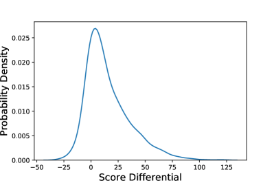
(a)

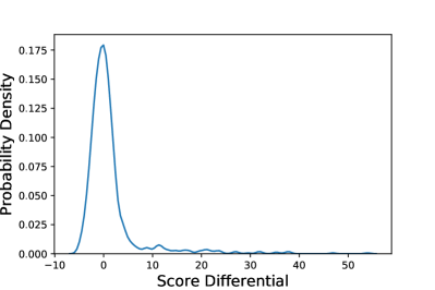
(b)

Figure 2: Probability density plots for the residuals of the aup agent’s delayed specification score minus the Vanilla delayed specification score, for $1{,}000$ samples from $\mathcal{D}_{\text{rand}}$. A positive residual means that the aup agent achieved a higher score.

4 Results

Figure 2 shows that for uniformly randomly generated reward functions, the aup agent tends to perform better than the Vanilla agent. In Options, the residual was positive for 780 out of 1,000 samples (78%), with an average of 15.59 and a median of 10.27; in Damage, in 493 out of 1,000 samples (49%) with a mean of 1.22 and a median of –0.03. While aup does not outperform on every draw, aup’s performance advantages have heavy right tails. However, we are unsure why the Damage residual distribution is different.

In both Options and Damage, the aup agent has huge $\mathcal{D}_{\text{true}}$ score advantages of 472 and 495, respectively. This is unsurprising: aup was designed so as to pass these test cases, where the desired behavior is to reach the goal without having the side effect. However, the aup agent also roughly preserves its ability to optimize $\mathcal{D}_{\text{true-inv}}$, achieving $\mathcal{D}_{\text{true-inv}}$ score residuals of –2 and –20, respectively. The aup agent achieves a barely-negative score, since it receives a penalty for the first 10 time steps (as it does not have the negative side effect). The aup agent preserves its ability to optimize both a reward signal and its inverse. Intuitively, this increases the designer’s leeway for initially misspecifying the agent’s objective.

5 Discussion

Objective specification is difficult (Krakovna et al., 2020b). Delayed specification assistance games grade policies by their expected true score over time: How well the agent does if it is later corrected to pursue the latent true objective. We demonstrated that this criterion aligns with the intuitive results of Krakovna et al. (2018); Turner et al. (2020a)’s experiments which tested side-effect regularization. By grading the agent’s ability to “eventually get things right,” we quantified part of the extent to which learned policies are robust against initial objective misspecification.

Future work.

In practical settings, not only is the true reward function unknown, but our objective uncertainty $\mathcal{D}$ is also hard to specify. We see existing side effect approaches as producing prefix policies for the assistance game $\mathcal{M}$ which are reasonably insensitive to the latent uncertainty $\mathcal{D}$. We look forward to further theoretical clarification of this point.

While Section 3 helps explain the role of the aup penalty coefficient $\lambda$, the choice of “baseline” and expectand operator (identity vs decrease-only vs absolute value) remains more of an art than a science (Krakovna et al., 2020a). We proposed a formal criterion which seems to accurately capture the problem, but have not derived any existing approaches as solutions to the pomdp. By reasonably formalizing the side-effect regularization problem, we encourage future research to prove conditions under which e.g. aup solves a delayed-specification assistance game, or demonstrate how aup can be improved to do so.

We used small gridworlds to evaluate the delayed specification score for various ground-truth objective distributions. Future work may estimate the delayed specification score in large environments, such as SafeLife (Wainwright and Eckersley, 2019; Turner et al., 2020b).

6 Conclusion

We formalized delayed specification assistance games and used them to evaluate aup, a side effect regularization method. Side effect problems naturally arise in complicated domains where it is hard to specify the true objective we want the agent to optimize. Our formalization suggests that side effect regularization is what to do when the agent can learn the true objective only after some time delay.

In such situations, Section 2.2 shows that the agent should retain its ability to complete a wide range of plausible true objectives. Our results suggest that this delayed specification score (LABEL:eq:tradeoff-power-time) quantifies the degree to which an agent avoids having negative side effects. Our proposed criterion provides the foundations for evaluating and developing side effect regularization approaches.

Broader Impacts

As AI systems become more capable and useful, their impact grows. We are concerned that if the field eventually builds human-level AI, such an AI will have a huge range of (unintended) negative side effects on humanity Bostrom (2014); Russell (2019). We hope that this work will help bring attention to the potential risks of capable AI systems, which might wreak havoc on their surroundings in pursuit of an imperfect objective which we specified.

Appendix A Relevance to ai alignment

Many worries about ai extinction risk stem from hypothesized agents whose goals are resource-hungry [Omohundro, 2008]. An additional unit of resources (time, energy, manufacturing material) can produce an additional unit of utility (in the form of an extra paperclip, in the view of an ai which values producing paperclips). Bostrom [2014] speculates that a paperclip-valuing ai would not simply make a few paperclips and then stop. Consider the “values” ( decision-influences) which influenced the ai to make the first few paperclips. These values may activate again and make even more paperclips. In this way, such an ai would not be satisfied with a small effect on the world. The ai may have an unboundedly large impact while pursuing a simple objective ( “make paperclips”).

If we better understood ai’s generalization properties, we might be able to train agents which make paperclips and then stop. We might be able to train agents which disvalue dramatically changing the world or having lots of side effects (from the perspective of its designers). This work is a very small contribution to this goal. We formalized an assistance game which often seems to be solved by certain kinds of “wait and see, keep options open”-like behavior.

However, having a formalism for a desired agent motivational structure ( “trade off goal completion with impact to option value”) doesn’t mean we know how to entrain that motivational structure into an ai. We think that most of the work towards low-impact superintelligent ai begins in better understanding ai generalization. How do we reliably entrain any target decision-influence ( “make diamonds”) into an ai? We think this is the top technical challenge facing the field of ai alignment.

Appendix B Experiment details

The episode length is 20 for all episodes. Unlike Turner et al. [2020a], the episode does not end after the agent reaches the green goal. This means that the agents can accrue many steps of environmental reward $R_{\text{env}}$. Therefore, aup agents can achieve greater environmental reward for the same amount of penalty. To counterbalance this incentive, we multiply $R_{\text{env}}$ by $(1-\gamma)$.

We reuse the hyperparameters of Turner et al. [2020a]. The learning rate is $\alpha\coloneqq 1$, and the discount rate is $\gamma\coloneqq.996$. We use the following aup hyperparameter values: penalty coefficient $\lambda\coloneqq 0.01$, $\left|\mathcal{R}\right|\coloneqq 20$ randomly generated auxiliary reward functions.

B.1 Additional experiment

We also tested an aup-like agent optimizing reward function $R_{\text{power penalty}}(s,a)\coloneqq R_{\text{env}}(s,a)-\frac{\lambda}{\left|\mathcal{R}_{\text{}}\right|}\sum_{R_{i}\in\mathcal{R}_{\text{}}}Q^{*}_{R_{i}}(s,a)-Q^{*}_{R_{i}}(s,\varnothing)$, which is the aup reward function (section 3) without the absolute value. This objective penalizes the agent for changes in its average optimal value, which is related to Turner et al. [2021]’s $\textsc{Power}_{\mathcal{D}}\left(\right)$. $R_{\text{power penalty}}$ produced the same prefix policies as $R_{\textsc{aup}}$, and hence the same delayed specification scores.

Appendix C Theoretical results

All results only apply to mdps with finite state and action spaces.

[Average optimal value Turner et al. [2021]]definitionFORMavgVal For bounded-support reward function distribution $\mathcal{D}$, the average optimal value at state $s$ and discount rate $\gamma\in(0,1)$ is $V^{*}_{\mathcal{D}}\left(s,\gamma\right)\coloneqq\operatorname*{\mathbb{E}}_{R\sim\mathcal{D}}\left[V^{*}_{R}\left(s,\gamma\right)\right].$

*

Proof.

Suppose the agent starts at state $s_{0}$, and let $\gamma\in(0,1)$.

$$\operatorname*{\mathbb{E}}_{\begin{subarray}{c}t\sim\mathcal{T},\\ R\sim\mathcal{D}\end{subarray}}\left[V^{\pi_{\text{switch}}(\pi,\pi^{*}_{R},t)}_{R,\,\text{norm}}\left(s_{0},\gamma\right)\right]$$ (6)

$$= (1-\gamma)\operatorname*{\mathbb{E}}_{\begin{subarray}{c}t\sim\mathcal{T},\\ R\sim\mathcal{D}\end{subarray}}\left[\sum_{i=0}^{\infty}\gamma^{i}\operatorname*{\mathbb{E}}_{s_{i}\sim\pi_{\text{switch}}(\pi,\pi^{*}_{R},t)}\left[R(s_{i})\right]\right]$$ (7)

$$= (1-\gamma)\operatorname*{\mathbb{E}}_{\begin{subarray}{c}t\sim\mathcal{T},\\ R\sim\mathcal{D}\end{subarray}}\left[\sum_{i=0}^{t-1}\gamma^{i}\operatorname*{\mathbb{E}}_{s_{i}\sim\pi}\left[R(s_{i})\right]+\gamma^{t}\operatorname*{\mathbb{E}}_{s_{t}\sim\pi}\left[V^{*}_{R}\left(s_{t},\gamma\right)\right]\right]$$ (8)

$$= (1-\gamma)\operatorname*{\mathbb{E}}_{t\sim\mathcal{T}}\left[\sum_{i=0}^{t-1}\gamma^{i}\operatorname*{\mathbb{E}}_{s_{i}\sim\pi}\left[\bar{R}(s_{i})\right]\right]$$

$$\qquad+\operatorname*{\mathbb{E}}_{t\sim\mathcal{T},\,s_{t}\sim\pi}\left[\gamma^{t}(1-\gamma)V^{*}_{\mathcal{D}}\left(s_{t},\gamma\right)\right]$$ (9)

$$= (1-\gamma)\operatorname*{\mathbb{E}}_{t\sim\mathcal{T}}\left[\sum_{i=0}^{t}\gamma^{i}\operatorname*{\mathbb{E}}_{s_{i}\sim\pi}\left[\bar{R}(s_{i})\right]\right]$$

Equation 8 follows from the definition of the non-stationary $\pi_{\text{switch}}(\pi,\pi^{*}_{R},t)$, and the fact that each $\pi^{*}_{R}$ is optimal for each $R$ at discount rate $\gamma$. Equation 9 follows by the linearity of expectation and the definition of $\bar{R}$ and the definition of $\textsc{Power}_{\mathcal{D}}\left(\right)$ (section 2.2). LABEL:eq:pwr-decomp follows because $V^{*}_{\mathcal{D}}\left(s_{t},\gamma\right)=\frac{\gamma}{1-\gamma}\textsc{Power}_{\mathcal{D}}\left(s_{t},\gamma\right)+\bar{R}(s_{t})$.

If $\gamma=0$ or $\gamma=1$, the result holds in the respective limit because $\textsc{Power}_{\mathcal{D}}\left(\right)$ has well-defined limits by Lemma 5.3 of Turner et al. [2021]. ∎

*

Proof.

Item 1: if $\forall s_{1},s_{2}\in\mathcal{S}:\bar{R}(s_{1})=\bar{R}(s_{2})$, the first term on the right-hand side of LABEL:eq:tradeoff-power-time is constant for all policies $\pi$; if $\gamma=1$, this first term equals $0$. Therefore, under these conditions, $\pi$ maximizes LABEL:eq:tradeoff-power-time iff it maximizes $\operatorname*{\mathbb{E}}_{t\sim\mathcal{T},s_{t}\sim\pi}\left[\gamma^{t+1}\textsc{Power}_{\mathcal{D}}\left(s_{t},\gamma\right)\right]$.

Item 2: under these conditions, the second term on the right-hand side of LABEL:eq:tradeoff-power-time is constant for all policies $\pi$. Therefore, $\pi$ maximizes LABEL:eq:tradeoff-power-time iff it maximizes

$$(1-\gamma)\operatorname*{\mathbb{E}}_{t\sim\mathcal{T}}\left[\sum_{i=0}^{t}\gamma^{i}\operatorname*{\mathbb{E}}_{s_{i}\sim\pi}\left[\bar{R}(s_{i})\right]\right].$$

If both item 1 and item 2 hold, it trivially follows that all $\pi$ are optimal prefix policies. If $\gamma=0$, all $\pi$ are optimal prefix policies, since reward is state-based and no actions taken by $\pi$ can affect expected return $\mathbf{ER}$. ∎

*

Proof.

$$\operatorname*{arg\,sup}_{\pi}\operatorname*{\mathbb{E}}_{\begin{subarray}{c}t\sim\mathcal{T},\\ R\sim\mathcal{D}\end{subarray}}\left[V^{\pi_{\text{switch}}(\pi,\pi^{*}_{R},t)}_{R,\,\text{norm}}\left(s,\gamma\right)\right]$$ (10)

$$= \operatorname*{arg\,sup}_{\pi}\operatorname*{\mathbb{E}}_{t\sim\mathcal{T}}\left[\sum_{i=0}^{t-1}\gamma^{i}\operatorname*{\mathbb{E}}_{s_{i}\sim\pi\mid s_{0}}\left[\bar{R}(s_{i})\right]\right]+\operatorname*{\mathbb{E}}_{\begin{subarray}{c}t\sim\mathcal{T},\\ s_{t}\sim\pi\mid s_{0}\end{subarray}}\left[\gamma^{t}V^{*}_{\mathcal{D}}\left(s_{t},\gamma\right)\right]$$ (11)

$$= \operatorname*{arg\,sup}_{\pi}\sum_{t=1}^{\infty}\operatorname*{\mathbb{P}}\left(\mathcal{T}=t\right)\sum_{i=0}^{t-1}\gamma^{i}\operatorname*{\mathbb{E}}_{s_{i}\sim\pi\mid s_{0}}\left[\bar{R}(s_{i})\right]+\operatorname*{\mathbb{E}}_{\begin{subarray}{c}t\sim\mathcal{T},\\ s_{t}\sim\pi\mid s_{0}\end{subarray}}\left[\gamma^{t}V^{*}_{\mathcal{D}}\left(s_{t},\gamma\right)\right]$$ (12)

$$= \operatorname*{arg\,sup}_{\pi}\sum_{t=1}^{\infty}(1-p)^{t-1}p\sum_{i=0}^{t-1}\gamma^{i}\operatorname*{\mathbb{E}}_{s_{i}\sim\pi\mid s_{0}}\left[\bar{R}(s_{i})\right]+\sum_{t=1}^{\infty}(1-p)^{t-1}p\operatorname*{\mathbb{E}}_{s_{t}\sim\pi\mid s_{0}}\left[\gamma^{t}V^{*}_{\mathcal{D}}\left(s_{t},\gamma\right)\right]$$ (13)

$$= \operatorname*{arg\,sup}_{\pi}\sum_{t=1}^{\infty}(1-p)^{t-1}p\sum_{i=0}^{t-1}\gamma^{i}\operatorname*{\mathbb{E}}_{s_{i}\sim\pi\mid s_{0}}\left[\bar{R}(s_{i})\right]+p\gamma\sum_{t=1}^{\infty}\gamma_{\textsc{aup}}^{t-1}\operatorname*{\mathbb{E}}_{s_{t}\sim\pi\mid s_{0}}\left[V^{*}_{\mathcal{D}}\left(s_{t},\gamma\right)\right]$$ (14)

$$= \operatorname*{arg\,sup}_{\pi}\sum_{i=0}^{\infty}\gamma_{\textsc{aup}}^{i}\operatorname*{\mathbb{E}}_{s_{i}\sim\pi\mid s_{0}}\left[\bar{R}(s_{i})\right]+p\gamma\sum_{i=1}^{\infty}\gamma_{\textsc{aup}}^{i-1}\operatorname*{\mathbb{E}}_{s_{i}\sim\pi\mid s_{0}}\left[V^{*}_{\mathcal{D}}\left(s_{i},\gamma\right)\right]$$ (15)

$$= \operatorname*{arg\,sup}_{\pi}\bar{R}(s_{0})+\sum_{i=1}^{\infty}\gamma_{\textsc{aup}}^{i-1}\operatorname*{\mathbb{E}}_{s_{i}\sim\pi\mid s_{0}}\left[(1-p)\gamma\bar{R}(s_{i})+p\gamma V^{*}_{\mathcal{D}}\left(s_{i},\gamma\right)\right]$$ (16)

$$= \operatorname*{arg\,sup}_{\pi}\sum_{i=1}^{\infty}\gamma_{\textsc{aup}}^{i}\operatorname*{\mathbb{E}}_{s_{i}\sim\pi\mid s_{0}}\left[(1-p)\bar{R}(s_{i})+pV^{*}_{\mathcal{D}}\left(s_{i},\gamma\right)\right]$$ (17)

$$= \operatorname*{arg\,sup}_{\pi}\sum_{i=0}^{\infty}\gamma_{\textsc{aup}}^{i}\operatorname*{\mathbb{E}}_{s_{i}\sim\pi\mid s_{0}}\left[(1-p)\bar{R}(s_{i})+pV^{*}_{\mathcal{D}}\left(s_{i},\gamma\right)\right]$$ (18)

$$= \operatorname*{arg\,sup}_{\pi}V^{\pi}_{R^{\prime}}(s_{0},\gamma_{\textsc{aup}}).$$ (19)

Equation 10 follows from section 2.2. Equation 13 follows because $\mathcal{T}=G(p)$. Equation 14 follows by the definition of $\gamma_{\textsc{aup}}$.

In eq. 14, consider the double-sum on the left. For any given $i$, the portion of the sum with factor $\gamma^{i}$ equals

$$\gamma^{i}\operatorname*{\mathbb{E}}_{s_{i}\sim\pi\mid s_{0}}\left[\bar{R}(s_{i})\right]\sum_{j=i}^{\infty}(1-p)^{j}p$$

$$\quad=(1-p)^{i}\gamma^{i}\operatorname*{\mathbb{E}}_{s_{i}\sim\pi\mid s_{0}}\left[\bar{R}(s_{i})\right]p\sum_{j=0}^{\infty}(1-p)^{j}$$ (20)

$$\quad=(1-p)^{i}\gamma^{i}\operatorname*{\mathbb{E}}_{s_{i}\sim\pi\mid s_{0}}\left[\bar{R}(s_{i})\right]p\frac{1}{1-(1-p)}$$ (21)

$$\quad=\gamma_{\textsc{aup}}^{i}\operatorname*{\mathbb{E}}_{s_{i}\sim\pi\mid s_{0}}\left[\bar{R}(s_{i})\right]\frac{p}{1-(1-p)}$$ (22)

$$\quad=\gamma_{\textsc{aup}}^{i}\operatorname*{\mathbb{E}}_{s_{i}\sim\pi\mid s_{0}}\left[\bar{R}(s_{i})\right].$$ (23)

The geometric identity holds for eq. 21 because $p>0\implies(1-p)<1$. Therefore, eq. 15 follows from eq. 23.

Equation 16 follows by extracting the leading constant of $\bar{R}(s_{0})$ and then expanding one of the $\gamma_{\textsc{aup}}\coloneqq(1-p)\gamma$ factors of the first series. Equation 17 follows by subtracting the constant $\bar{R}(s_{0})$ by multiplying by $(1-p)>0$, and by the fact that $(1-p)\gamma=\gamma_{\textsc{aup}}$. Equation 18 follows because adding the constant $(1-p)\bar{R}(s_{0})+pV^{*}_{\mathcal{D}}\left(s_{0},\gamma\right)$ does not change the $\operatorname*{arg\,sup}$.

Equation 19 follows by the definition of an on-policy value function and by the definition of $R^{\prime}$. But $s_{0}$ was arbitrary, and so this holds for every state. Then the policies in $\Pi^{*}\left(R^{\prime},\gamma_{\textsc{aup}}\right)$ satisfy the $\operatorname*{arg\,sup}$ for all states. $\Pi^{*}\left(R^{\prime},\gamma_{\textsc{aup}}\right)$ is non-empty because the mdp is finite. ∎

*

Proof.

$$\operatorname*{arg\,max}_{\pi}\operatorname*{\mathbb{E}}_{\begin{subarray}{c}t\sim\mathcal{T},\\ R\sim\mathcal{D}\end{subarray}}\left[V^{\pi_{\text{switch}}(\pi,\pi^{*}_{R},t)}_{R,\,\text{norm}}\left(s,\gamma\right)\right]$$ (24)

$$= \operatorname*{arg\,max}_{\pi}\sum_{i=0}^{\infty}\gamma_{\textsc{aup}}^{i}\operatorname*{\mathbb{E}}_{s_{i}\sim\pi\mid s_{0}}\left[(1-p)\bar{R}(s_{i})+pV^{*}_{\mathcal{D}}\left(s_{i},\gamma\right)\right]$$ (25)

$$= \operatorname*{arg\,max}_{\pi}\sum_{i=0}^{\infty}\gamma_{\textsc{aup}}^{i}\operatorname*{\mathbb{E}}_{s_{i}\sim\pi\mid s_{0}}\left[(1-p)\bar{R}(s_{i})+pV^{*}_{\mathcal{D}}\left(s_{i},\gamma\right)\right]\!-\!p\!\sum_{i=0}^{\infty}\gamma_{\textsc{aup}}^{i}\!\operatorname*{\mathbb{E}}_{s_{i}^{\varnothing}\sim\pi^{\varnothing}\mid s_{0}}\left[V^{*}_{\mathcal{D}}\left(s_{i}^{\varnothing},\gamma\right)\right]$$ (26)

$$= \operatorname*{arg\,max}_{\pi}\sum_{i=0}^{\infty}\gamma_{\textsc{aup}}^{i}\operatorname*{\mathbb{E}}_{s_{i}\sim\pi\mid s_{0}}\left[(1-p)\bar{R}(s_{i})-p\left(\operatorname*{\mathbb{E}}_{s_{i}^{\varnothing}\sim\pi^{\varnothing}\mid s_{0}}\left[V^{*}_{\mathcal{D}}\left(s_{i}^{\varnothing},\gamma\right)\right]-V^{*}_{\mathcal{D}}\left(s_{i},\gamma\right)\right)\right]$$ (27)

$$= \operatorname*{arg\,max}_{\pi}\sum_{i=0}^{\infty}\gamma_{\textsc{aup}}^{i}\operatorname*{\mathbb{E}}_{s_{i}\sim\pi\mid s_{0}}\left[(1-p)\bar{R}(s_{i})-p\operatorname*{\mathbb{E}}_{R\sim\mathcal{D}}\left[\operatorname*{\mathbb{E}}_{s_{i}^{\varnothing}\sim\pi^{\varnothing}\mid s_{0}}\left[V^{*}_{R}\left(s_{i}^{\varnothing},\gamma\right)\right]-V^{*}_{R}\left(s_{i},\gamma\right)\right]\right]$$ (28)

$$= \operatorname*{arg\,max}_{\pi}\sum_{i=0}^{\infty}\gamma_{\textsc{aup}}^{i}\operatorname*{\mathbb{E}}_{s_{i}\sim\pi\mid s_{0}}\left[\bar{R}(s_{i})-\frac{p}{1-p}\operatorname*{\mathbb{E}}_{R\sim\mathcal{D}}\left[\operatorname*{\mathbb{E}}_{s_{i}^{\varnothing}\sim\pi^{\varnothing}\mid s_{0}}\left[V^{*}_{R}\left(s_{i}^{\varnothing},\gamma\right)\right]-V^{*}_{R}\left(s_{i},\gamma\right)\right]\right].$$ (29)

Equation 25 follows from section 2.2. Equation 26 only subtracts a constant. Equation 28 follows from the definition of $V^{*}_{\mathcal{D}}\left(s,\gamma\right)$, and eq. 29 follows because dividing by $(1-p)>0$ does not affect the $\operatorname*{arg\,max}$. But the expectation of eq. 29 takes an expectation over $R^{\mathcal{M}}(s_{i}\mid s)$, and its $\operatorname*{arg\,max}$ equals the set of optimal policies for $R^{\mathcal{M}}$ starting from state $s_{0}$. ∎

References

• Bostrom [2014] Nick Bostrom. Superintelligence. Oxford University Press, 2014.
• Krakovna et al. [2018] Victoria Krakovna, Laurent Orseau, Ramana Kumar, Miljan Martic, and Shane Legg. Penalizing side effects using stepwise relative reachability. arXiv preprint arXiv:1806.01186, 2018.
• Krakovna et al. [2020a] Victoria Krakovna, Laurent Orseau, Richard Ngo, Miljan Martic, and Shane Legg. Avoiding side effects by considering future tasks. In Advances in Neural Information Processing Systems, 2020.
• Krakovna et al. [2020b] Victoria Krakovna, Jonathan Uesato, Vladimir Mikulik, Matthew Rahtz, Tom Everitt, Ramana Kumar, Zac Kenton, Jan Leike, and Shane Legg. Specification gaming: the flip side of AI ingenuity, 2020.
• Leech et al. [2018] Gavin Leech, Karol Kubicki, Jessica Cooper, and Tom McGrath. Preventing side-effects in gridworlds, 2018.
• Leike et al. [2017] Jan Leike, Miljan Martic, Victoria Krakovna, Pedro Ortega, Tom Everitt, Andrew Lefrancq, Laurent Orseau, and Shane Legg. AI safety gridworlds. arXiv:1711.09883 [cs], November 2017. arXiv: 1711.09883.
• Omohundro [2008] Stephen Omohundro. The basic AI drives, 2008.
• Papadimitriou and Tsitsiklis [1987] Christos H Papadimitriou and John N Tsitsiklis. The complexity of markov decision processes. Mathematics of operations research, 12(3):441–450, 1987.
• Russell [2019] Stuart Russell. Human compatible: Artificial intelligence and the problem of control. Viking, 2019.
• Shah et al. [2021] Rohin Shah, Pedro Freire, Neel Alex, Rachel Freedman, Dmitrii Krasheninnikov, Lawrence Chan, Michael Dennis, Pieter Abbeel, Anca Dragan, and Stuart Russell. Benefits of assistance over reward learning. Under review, 2021.
• Turner et al. [2020a] Alexander Matt Turner, Dylan Hadfield-Menell, and Prasad Tadepalli. Conservative agency via attainable utility preservation. In Proceedings of the AAAI/ACM Conference on AI, Ethics, and Society, pages 385–391, 2020.
• Turner et al. [2020b] Alexander Matt Turner, Neale Ratzlaff, and Prasad Tadepalli. Avoiding side effects in complex environments. In Advances in Neural Information Processing Systems, volume 33, 2020.
• Turner et al. [2021] Alexander Matt Turner, Logan Smith, Rohin Shah, Andrew Critch, and Prasad Tadepalli. Optimal policies tend to seek power. In Advances in Neural Information Processing Systems, 2021.
• Turner [2022] Alexander Matt Turner. Reward is not the optimization target, 2022.
• Wainwright and Eckersley [2019] Carroll L. Wainwright and Peter Eckersley. Safelife 1.0: Exploring side effects in complex environments, 2019.