Algorithms for 2-connected network design and flexible Steiner trees with a constant number of terminals

Abstract

The $k$-Steiner-2NCS problem is as follows: Given a constant $k$, and an undirected connected graph $G=(V,E)$, non-negative costs $c$ on the edges, and a partition $(T,V\setminus{T})$ of $V$ into a set of terminals, $T$, and a set of non-terminals (or, Steiner nodes), where $|T|=k$, find a min-cost two-node connected subgraph that contains the terminals.

We present a randomized polynomial-time algorithm for the unweighted problem, and a randomized FPTAS for the weighted problem.

We obtain similar results for the $k$-Steiner-2ECS problem, where the input is the same, and the algorithmic goal is to find a min-cost two-edge connected subgraph that contains the terminals.

Our methods build on results by Björklund, Husfeldt, and Taslaman (SODA 2012) that give a randomized polynomial-time algorithm for the unweighted $k\text{-}\mathrm{Steiner}\text{-}\mathrm{cycle}$ problem; this problem has the same inputs as the unweighted $k$-Steiner-2NCS problem, and the algorithmic goal is to find a min-cost simple cycle $C$ that contains the terminals ($C$ may contain any number of Steiner nodes).

Introduction

We address the following open question in the area of network design: Is there a polynomial-time algorithm for the $k\text{-}\mathrm{Steiner}\text{-}\mathrm{2NCS}$ problem (where the number of terminals, denoted by $k$, is a constant)? The input is an undirected connected graph $G=(V,E)$, non-negative costs $c$ on the edges, and a partition $(T,V\setminus{T})$ of $V$ into terminals ($T$) and non-terminals (or, Steiner nodes). The algorithmic goal is to find a min-cost two-node connected subgraph that contains the terminals. See Feldman et al. [7], the third item in the last section (open problems), and for related results, see [11, 6].

We present a randomized polynomial-time algorithm for the unweighted $k\text{-}\mathrm{Steiner}\text{-}\mathrm{2NCS}$ problem, and a randomized FPTAS for the weighted problem.

We obtain similar results for the $k\text{-}\mathrm{Steiner}\text{-}\mathrm{2ECS}$ problem, where the input is the same, and the algorithmic goal is to find a min-cost two-edge connected subgraph that contains the terminals, see Section 5. In fact we address a generalization of the $k\text{-}\mathrm{Steiner}\text{-}\mathrm{2ECS}$ problem called the k-Flexible Steiner Tree problem ($k\text{-}\mathrm{FST}$): The input consists of an undirected graph $G=(V,E)$ with nonnegative costs on the edges $c\in\mathbb{R}_{\geq 0}^{E}$, a partition of the edge-set $E$ into a set $\mathscr{S}$ of safe edges and a set $\mathscr{U}$ of unsafe edges, and a subset of the nodes $T\subseteq V$ with $|T|=k$, called the terminals. The algorithmic goal is to find a connected subgraph $H=(U,F)$ of minimum cost (i.e., minimizing $c(F)$) such that $T\subseteq{U}$ and for any unsafe edge $e\in{F}$, the graph $H-e$ is connected. Clearly, the $k\text{-}\mathrm{Steiner}\text{-}\mathrm{2ECS}$ problem is a special case of $k\text{-}\mathrm{FST}$ where all edges are unsafe.

Our methods build on results by Björklund, Husfeldt, and Taslaman (SODA 2012) [2] that give a randomized polynomial-time algorithm for the unweighted $k\text{-}\mathrm{Steiner}\text{-}\mathrm{cycle}$ problem; this problem has the same inputs as the $k\text{-}\mathrm{Steiner}\text{-}\mathrm{2NCS}$ problem, and the algorithmic goal is to find a min-cost simple cycle $C$ that contains the terminals ($C$ may contain any number of Steiner nodes). To the best of our knowledge, no polynomial-time (deterministic or randomized) algorithm is known for finding an optimal solution of the weighted $k\text{-}\mathrm{Steiner}\text{-}\mathrm{cycle}$ problem, even for $k=3$; this problem has been open for several decades, see [4]. There are a number of related results from the last few decades; for example, see [8, 3].

The randomized polynomial-time algorithm for the unweighted $k\text{-}\mathrm{Steiner}\text{-}\mathrm{cycle}$ problem of [2] extends easily to a randomized FPTAS for the weighted $k\text{-}\mathrm{Steiner}\text{-}\mathrm{cycle}$ problem, by using techniques from Ibarra & Kim [10] and Hochbaum & Shmoys [9], see Proposition 3. Our randomized FPTAS results (discussed above) use the same methods, see Corollaries 8 and 13.

Preliminaries

This section has definitions and preliminary results. Our notation and terms are consistent with [5], and readers are referred to that text for further information.

Let $G=(V,E)$ be a (loop-free) multi-graph with non-negative costs $c\in\mathbb{R}_{\geq 0}^{E}$ on the edges. We take $G$ to be the input graph, and we use $n$ to denote $|V(G)|$. For a set of edges $F\subseteq E(G)$, $c(F):=\sum_{e\in F}c(e)$, and for a subgraph $G^{\prime}$ of $G$, $c(G^{\prime}):=\sum_{e\in E(G^{\prime})}c(e)$.

For a positive integer $k$, we use $[k]$ to denote the set $\{1,\dots,k\}$.

For a graph $H$ and a set of nodes $S\subseteq V(H)$, $\Gamma_{H}(S):=\{w\in{V(H)\setminus S}\,:\,v\in{S},vw\in{E(H)}\}$, thus, $\Gamma_{H}(S)$ denotes the set of neighbours of $S$.

For a graph $H$ and a set of nodes $S\subseteq V(H)$, $\delta_{H}(S)$ denotes the set of edges that have one end node in $S$ and one end node in $V(H)\setminus S$; moreover, $H[S]$ denotes the subgraph of $H$ induced by $S$, and $H-S$ denotes the subgraph of $H$ induced by $V(H)\setminus S$. For a graph $H$ and a set of edges $F\subseteq E(H)$, $H-F$ denotes the graph $(V(H),\leavevmode\nobreak\ E(H)\setminus F)$. We may use relaxed notation for singleton sets, e.g., we may use $\delta_{H}(v)$ instead of $\delta_{H}(\{v\})$, and we may use $H-v$ instead of $H-\{v\}$, etc.

We may not distinguish between a subgraph and its node set; for example, given a graph $H$ and a set $S$ of its nodes, we use $E(S)$ to denote the edge set of the subgraph of $H$ induced by $S$.

2.1 2EC, 2NC and related notions

A multi-graph $H$ is called $k$-edge connected if $|V(H)|\geq 2$ and for every $F\subseteq E(H)$ of size $<k$, $H-F$ is connected. Thus, $H$ is 2-edge connected if it has $\geq 2$ nodes and the deletion of any one edge results in a connected graph. A multi-graph $H$ is called $k$-node connected if $|V(H)|>k$ and for every $S\subseteq V(H)$ of size $<k$, $H-S$ is connected. We use the abbreviations 2EC for “2-edge connected,” and 2NC for “2-node connected.”

For any instance $H$, we use $\textsc{opt}(H)$ to denote the minimum cost of a feasible subgraph (i.e., a subgraph that satisfies the requirements of the problem). When there is no danger of ambiguity, we use opt rather than $\textsc{opt}(H)$.

By a bridge we mean an edge of a connected (sub)graph whose removal results in two connected components, and by a cut-node we mean a node of a connected (sub)graph whose deletion results in two or more connected components. A maximal connected subgraph without a cut-node is called a block. Thus, every block of a given graph $G$ is either a maximal 2NC subgraph, or a bridge (and its incident nodes), or an isolated node. For any node $v$ of $G$, let $\Gamma^{\mathit{blocks}}_{G}(v)$ denote the set of 2NC blocks of $G$ that contain $v$.

2.2 Ear decompositions

An ear decomposition of a graph is a partition of the edge set into paths or cycles, $P_{0},P_{1},\dots,P_{\ell}$, such that $P_{0}$ is the trivial path with one node, and each $P_{i}$ ($1\leq i\leq{\ell}$) is either (1) a path that has both end nodes in $V_{i-1}=V(P_{0})\cup V(P_{1})\cup\ldots\cup V(P_{i-1})$ but has no internal nodes in $V_{i-1}$, or (2) a cycle that has exactly one node in $V_{i-1}$. For an ear $P_{i}$, let $\mathrm{int}(P_{i})$ denote the set of nodes $V(P_{i})\setminus{V_{i-1}}$. Each of $P_{1},\ldots,P_{\ell}$ is called an ear; note that $P_{0}$ is not regarded as an ear. We call $P_{i},i\in\{1,\dots,{\ell}\},$ an open ear if it is a path, and we call it a closed ear if it is a cycle. An open ear decomposition $P_{0},P_{1},\ldots,P_{\ell}$ is one such that all the ears $P_{2},\ldots,P_{\ell}$ are open. (The ear $P_{1}$ is always closed.)

Proposition 1 (Whitney [13]).

• A graph is 2EC $\iff$ it has an ear decomposition.

• A graph is 2NC $\iff$ it has an open ear decomposition.

2.3 Algorithms for basic computations

There are well-known polynomial-time algorithms for implementing all of the basic computations in this paper, see [12]. We state this explicitly in all relevant results, but we do not elaborate on this elsewhere.

FPTAS for $k\text{-}\mathrm{Steiner}\text{-}\mathrm{cycle}$

Björklund, Husfeldt, and Taslaman [2] presented a randomized algorithm for finding a min-cost simple cycle that contains a given set of terminals $T$ of an unweighted, undirected graph $G=(V,E)$ with a running time of $2^{k}n^{O(1)}$, where $k=|T|$ and $n=|V|$. In other words, they present a randomized $\mathbf{FPT}$-algorithm for the unweighted $k\text{-}\mathrm{Steiner}\text{-}\mathrm{cycle}$ problem.

Theorem 2.

Consider a graph $G=(V,E)$ and a set of terminals $T\subseteq V$ of size $k$. Let $\eta>0$ be a parameter. A minimum-size $k\text{-}\mathrm{Steiner}\text{-}\mathrm{cycle}$ can be found, if one exists, by a randomized algorithm in time $2^{k}n^{O(1)}\log\frac{1}{\eta}$ with probability at least $1-\eta$.

We present a simple (randomized) FPTAS for the weighted $k\text{-}\mathrm{Steiner}\text{-}\mathrm{cycle}$ problem, based on the algorithm of [2].

Proposition 3.

Consider a graph $G=(V,E)$ with nonnegative costs $c\in\mathbb{R}_{\geq 0}^{E}$ on the edges, and a set of $k$ terminals $T\subseteq V$. Let $\varepsilon,\eta>0$ be some parameters. There is a randomized algorithm that finds a $(1+\varepsilon)$-approximate $k\text{-}\mathrm{Steiner}\text{-}\mathrm{cycle}$, if one exists, with probability at least $1-\eta$. The running time of the algorithm is $O\Bigl{(}2^{k}\cdot n^{O(1)}\cdot\bigl{(}\frac{1}{\varepsilon}\bigr{)}^{O(1)}\cdot\log\frac{1}{\eta}\Bigr{)}$.

Proof.

Let $E=\{e_{1},e_{2},\dots,e_{m}\}$ where $c_{e_{1}}\leq c_{e_{2}}\leq\dots\leq c_{e_{m}}$. Let $\eta^{\prime}:=\eta/2$. Let $j\in[m]$ denote the smallest index such that the graph $(V,\{e_{1},\dots,e_{j}\})$ contains a $k\text{-}\mathrm{Steiner}\text{-}\mathrm{cycle}$. Note that if $G$ does not have a $k\text{-}\mathrm{Steiner}\text{-}\mathrm{cycle}$, then the weighted-version of the problem is trivially infeasible. Using at most $m$ applications of Theorem 2 with the $\eta$-parameter set to $\eta^{\prime}$, we can find the index $j$ with probability at least $1-\eta/2$. Suppose that we have the correct index $j$. Let $\beta:=c(e_{j})$. Let $Q^{*}$ denote an optimal $k\text{-}\mathrm{Steiner}\text{-}\mathrm{cycle}$ in $G$, and $\textsc{opt}:=c(Q^{*})$ denote the optimal cost. By the definition of $j$, $\beta\leq\textsc{opt}\leq n\beta$. In particular, every edge in $Q^{*}$ has cost at most $n\beta$. We now describe our randomized algorithm for obtaining a $k\text{-}\mathrm{Steiner}\text{-}\mathrm{cycle}$ with cost at most $(1+\varepsilon)\textsc{opt}$. First, we discard all edges $e$ of $G$ with cost $c_{e}>n\,\beta$. Let $\mu:=\varepsilon\beta/n$; this is our “scaling parameter”. For each edge $e$, define $\tilde{c}_{e}:=\mu\cdot\max(1,\lceil c_{e}/\mu\rceil)$. Note that $\tilde{c}_{e}=\mu$ if $c_{e}=0$. (Observe that this rounding introduces errors, but the total error incurred on any cycle is $\leq n\,\mu\leq$ $\epsilon\beta\leq\epsilon\textsc{opt}$.) Consider the graph $\widetilde{G}=(\widetilde{V},\widetilde{E})$ obtained from $G$ by replacing each edge $e$ by a path of $\tilde{c}_{e}/\mu$ edges (of unit cost). Note that $|\widetilde{V}|\leq|V|+|E|\cdot(n\beta)/\mu=O(mn^{2}/\varepsilon)$. Using a single application of Theorem 2, we can obtain a minimum-size $k\text{-}\mathrm{Steiner}\text{-}\mathrm{cycle}$ $\widetilde{Q}\subseteq\widetilde{E}$ with probability at least $1-\eta/2$ in $O\Bigl{(}2^{k}\cdot\bigl{(}\frac{n^{2}m}{\varepsilon}\bigr{)}^{O(1)}\cdot\log\frac{1}{\eta}\Bigr{)}$ time. Let $Q$ denote the $k\text{-}\mathrm{Steiner}\text{-}\mathrm{cycle}$ in $G$ corresponding to $\widetilde{Q}$. By our choice of $\tilde{c}$, we have $c(Q)\leq\tilde{c}(Q)\leq\mu\cdot|\widetilde{Q}|$. Since the optimal $k\text{-}\mathrm{Steiner}\text{-}\mathrm{cycle}$ $Q^{*}$ consists of at most $n$ edges each with cost at most $n\beta$, the (unweighted) $k\text{-}\mathrm{Steiner}\text{-}\mathrm{cycle}$ $\widetilde{Q}^{*}$ in $\widetilde{G}$ corresponding to $Q^{*}$ satisfies $\mu|\widetilde{Q}^{*}|\leq\tilde{c}(Q^{*})\leq c(Q^{*})+n\mu\leq\textsc{opt}(1+\varepsilon)$. By the above discussion, we can obtain a $k\text{-}\mathrm{Steiner}\text{-}\mathrm{cycle}$ $Q$ satisfying $c(Q)\leq\mu|\widetilde{Q}|\leq\mu|\widetilde{Q}^{*}|\leq(1+\varepsilon)\textsc{opt}$ with probability at least $1-\eta$. Clearly, the overall running time is $O\Bigl{(}2^{k}\cdot n^{O(1)}\cdot\bigl{(}\frac{1}{\varepsilon}\bigr{)}^{O(1)}\cdot\log\frac{1}{\eta}\Bigr{)}$. ∎

FPTAS for $k\text{-}\mathrm{Steiner}\text{-}\mathrm{2NCS}$

Our (randomized) FPTAS for the $k\text{-}\mathrm{Steiner}\text{-}\mathrm{2NCS}$ problem is based on a lemma that describes the structure of a feasible subgraph, and it repeatedly applies the algorithm of [2] for $\mathrm{Steiner}\text{-}\mathrm{cycle}$. First, we present a randomized polynomial-time algorithm for finding an optimal subgraph for the special case of unweighted $k\text{-}\mathrm{Steiner}\text{-}\mathrm{2NCS}$; then, using the method from Section 3 we extend our algorithm to a (randomized) FPTAS for weighted $k\text{-}\mathrm{Steiner}\text{-}\mathrm{2NCS}$.

In this section, we denote an instance of the $k\text{-}\mathrm{Steiner}\text{-}\mathrm{2NCS}$ problem by $(G=(V,E),\,{c\in\mathbb{R}_{\geq 0}^{E}},\,T\subseteq{V})$; $G$ is the input graph with non-negative edge costs $c$, and $T$ is the set of terminals, $|T|\geq 3$ (we skip the easy case of $|T|=2$). We assume (w.l.o.g.) that $G$ is a feasible subgraph, that is, all terminals are contained in one block of $G$.

For any graph $H$, let $D_{3}(H)$ denote the set of nodes that have degree $\geq 3$ in $H$.

Lemma 4.

Let $H=(V^{\prime},E^{\prime})$ be an (edge) minimal 2NC subgraph that contains $T$. Then $H$ has an open ear decomposition $P_{0},P_{1},\dots,P_{\ell}$ such that
(i) each of the ears $P_{i}\leavevmode\nobreak\ (i\in[\ell])$ contains a terminal as an internal node (i.e., $\mathrm{int}(P_{i})\cap T\not=\emptyset$), and $P_{0}$ contains a terminal,
(ii) $|D_{3}(H)|\leq 2(|T|-2)$.

Proof.

(i) Pick any terminal to be $P_{0}$. Suppose we have constructed open ears $P_{1},\dots,P_{i-1}$ and that each $\mathrm{int}(P_{j})(j\in[i-1])$ contains a terminal. Let $F=\cup_{j=1}^{i-1}E(P_{j})$. Let $t$ be a terminal in $T\setminus{V(F)}$ (we have the required ear decomposition, if $T\subseteq V(F)$). Suppose $i=1$; then, $G$ has two openly disjoint paths between $t$ and $P_{0}$, and we take $P_{1}$ to be the edge-set of these two paths. Suppose $i\geq 2$; then, $G$ has a two-fan $P$ between $t$ and $V(F)$ (i.e., $P$ is the union of two paths between $t$ and $V(F)$ that have only the node $t$ in common); we take $P_{i}$ to be $P$.
(ii) Clearly, $\ell\leq|T|-1$ for the ear decomposition of (i), and each of the ears $P_{2},\dots,P_{\ell}$ contributes at most $2$ (new) nodes to $D_{3}(H)$. ∎

The next lemma states an extension of Proposition 1.

Lemma 5.

Let $G=(V,E)$ be a graph, and let $H=(V^{\prime},E^{\prime})$ be a 2NC subgraph of $G$. Let $P$ be a path of $G$ that has both end nodes in $V^{\prime}$. Then, $H\cup P=(V^{\prime}\cup V(P),E^{\prime}\cup E(P))$ is a 2NC subgraph of $G$.

Each set $S\subseteq{V}$ of size $\leq 2|T|-4$ is a candidate for $D_{3}(H)$ for a 2NC subgraph $H$ that contains $T$, and we call $T\cup{S}$ the set of marker nodes.

Our algorithm has several nested loops. The outer-most loop picks a set $S\subseteq{V}$ of size $\leq 2|T|-4$, and then applies the following main loop. Each iteration of the main loop attempts to construct a 2NC subgraph that contains the set of marker nodes $T\cup{S}$, by iterating over all ordered partitions $(\widetilde{T}_{1},\widetilde{T}_{2},\dots,\widetilde{T}_{r})$ of $T\cup{S}$ such that $|\widetilde{T}_{1}|\geq 2$ and the number of sets in the partition, $r$, is a positive integer, $r\leq{k}={|T|}$.

Consider one of these ordered partitions $(\widetilde{T}_{1},\widetilde{T}_{2},\dots,\widetilde{T}_{r})$. We attempt to find a min-cost $\mathrm{Steiner}\text{-}\mathrm{cycle}$ $C_{1}$ that contains $\widetilde{T}_{1}$ using the algorithm of [2]; if $G$ has no $\mathrm{Steiner}\text{-}\mathrm{cycle}$ that contains $\widetilde{T}_{1}$, then this iteration has failed, otherwise, we take $C_{1}$ to be the first (closed) ear of an open ear decomposition of our candidate 2NC subgraph that contains $T\cup{S}$. Then, for $i=1,\dots,r-1$, we pick a pair of nodes $s_{i},t_{i}\in\widetilde{T}_{1}\cup\dots\cup\widetilde{T}_{i}$, and attempt to find a min-cost $\mathrm{Steiner}\text{-}\mathrm{path}$ $P_{i+1}$ between $s_{i}$ and $t_{i}$ that contains $\widetilde{T}_{i+1}$; if $G$ has no such $\mathrm{Steiner}\text{-}\mathrm{path}$, then this iteration has failed, otherwise, we augment the current subgraph $H:=C_{1}\cup{P_{2}}\cup\dots\cup{P_{i}}$ by $P_{i+1}$.

The algorithm maintains an edge-set $\hat{F}$; initially, $\hat{F}=E$, and, at termination, $\hat{F}$ is the edge-set of a min-cost 2NC subgraph that contains $T$.

Pseudo-code for the algorithm is presented below.

We use $\mathcal{A}_{\text{BHT-cycle}}(G,\;\widetilde{T}_{1}{,\;\eta})$ to denote a call to the $\mathrm{Steiner}\text{-}\mathrm{cycle}$ algorithm of [2] where the inputs are the graph $G$, the terminal set $\widetilde{T}_{1}\subseteq V(G)$, and the desired probability of failure $\eta$. With probability at least $1-\eta$, this call either returns the edge-set of a minimum-size cycle of $G$ that contains all nodes of $\widetilde{T}_{1}$ or reports an error if $G$ has no such cycle.

We use $\mathcal{A}_{\text{BHT-path}}(G,\;\widetilde{T}_{1},\;s,\;t{,\;\eta})$ to denote a call to the following subroutine that attempts to find an $s,t$-path of $G$ that contains all nodes of $\widetilde{T}_{1}$. First, construct an auxiliary graph $G^{\prime}$ from $G$ by adding a node $u^{\prime}$ and two edges $u^{\prime}s,u^{\prime}t$. Then call $\mathcal{A}_{\text{BHT-cycle}}(G^{\prime},\;\widetilde{T}_{1}\cup\{u^{\prime},s,t\}{,\;\eta})$; report an error if the call returns an error, and, otherwise, return the path obtained by deleting the node $u^{\prime}$ (and its two incident edges) from the cycle returned by the call.

Algorithm $\mathcal{A}_{2NC}(G,\,T,\,\eta)$

(Set parameter) $\eta^{\prime}=\frac{\eta}{k}$;

(Initialize) $\hat{F}:=E$;

For $S\subseteq V$ such that $|S|\leq 2k$:

  For $r=1,\ldots,{k}$:

   For ordered partitions $(\widetilde{T}_{1},\ldots,\widetilde{T}_{r})$ of $T\cup S$ such that $|\widetilde{T}_{1}|\geq 2$:

    For $i=1,\ldots,r-1$ and node pairs $(s_{i},t_{i})\in\cup_{j=1}^{i}\widetilde{T}_{i}$, where $s_{i}\neq t_{i}$:

     $H:=\mathcal{A}_{\text{BHT-cycle}}(G,\widetilde{T}_{1}{,\;\eta^{\prime}})\quad\bigcup_{i=1}^{r-1}\mathcal{A}_{\text{BHT-path}}(G,\widetilde{T}_{i+1},s_{i},t_{i}{,\;\eta^{\prime}})$;

     Continue the loop if any call to any subroutine reports an error;

     If $|E(H)|<|\hat{F}|$, update $\hat{F}:=E(H)$;

    End For;

   End For;

  End For;

End For;

Output $\hat{F}$;

Lemma 6.

Let $H^{*}=(V^{*},E^{*})$ be an optimal subgraph for $k\text{-}\mathrm{Steiner}\text{-}\mathrm{2NCS}$. Assume that each of the calls to the subroutines (namely, $\mathcal{A}_{\text{BHT-cycle}},\mathcal{A}_{\text{BHT-path}}$) returns a valid subgraph whenever one exists. Let $H=(U,\hat{F})$ denote the output of the above algorithm. Then $H$ is a 2NC subgraph, $U\supseteq{T}$, and $|\hat{F}|\leq|E^{*}|=\textsc{opt}$.

Proof.

By Lemma 4, $H^{*}$ has an open ear decomposition $P_{1},P_{2},\ldots,P_{r^{*}}$ such that each of the ears $P_{i}$ contains at least one terminal as an internal node; hence, $r^{*}\leq k=|T|$. Let $S^{*}=D_{3}(H^{*})$ be the set of nodes of degree $\geq 3$ of $H^{*}$; clearly, $|S^{*}|\leq 2r^{*}\leq 2k$.

For $i=1,\ldots,r^{*}$, let $T^{*}_{i}=P_{i}\cap(T\cup S^{*})$. For $i=1,\ldots,r^{*}-1$, let $(s^{*}_{i},t^{*}_{i})$ denote the end nodes of the ear $P_{i+1}$; clearly, $(s_{i}^{*},t_{i}^{*})\in\cup_{j=1}^{i}(T_{i}^{*})$.

Now consider the loop in the algorithm where $S=S^{*}$, $r=r^{*}$, $\widetilde{T}_{i}=T^{*}_{i}$ for $i=1,\ldots,r^{*}$ and $(s_{i},t_{i})=(s^{*}_{i},t^{*}_{i})$ for $i=1,\ldots,r^{*}-1$. Observe that the calls to the subroutines $A_{\text{BHT-cycle}}$ and $\mathcal{A}_{\text{BHT-path}}$ return minimum-size subgraphs, hence, $|\mathcal{A}_{\text{BHT-cycle}}(G,\widetilde{T}_{1})|\leq|P_{1}|$ and $|\mathcal{A}_{\text{BHT-path}}(G,\widetilde{T}_{i+1},s_{i},t_{i})|\leq|P_{i+1}|$ for $i=1,\ldots,r^{*}-1$. Since $|E^{*}|=\sum_{i=1}^{r^{*}}|P_{i}|$, we conclude that the 2NC subgraph $H$ found by this iteration satisfies $|E(H)|\leq|E^{*}|$. Thus, the algorithm outputs an optimal 2NC subgraph that contains $T$. ∎

Theorem 7.

Consider the unweighted $k\text{-}\mathrm{Steiner}\text{-}\mathrm{2NCS}$ problem with $k=O(1)$. Let $\eta>0$ be a parameter. With probability $\geq 1-\eta$, the above randomized algorithm computes an optimal subgraph in time $O(\binom{n}{2k}\cdot B(3k)\cdot{\binom{3k}{2}^{k}}\cdot 2^{3k}n^{O(1)}\log{\frac{k}{\eta}})=O\left(n^{O(k)}\cdot\log{\frac{1}{\eta}}\right)$, where $B(i)$ denotes the $i^{th}$ ordered Bell number.

Proof.

As seen in the proof of Lemma 6, if the subroutines $A_{\text{BHT-cycle}}$ and $\mathcal{A}_{\text{BHT-path}}$ run correctly when $S=S^{*}$, $r=r^{*}$, $\widetilde{T}_{i}=T^{*}_{i}$ for $i=1,\ldots,r^{*}$ and $(s_{i},t_{i})=(s^{*}_{i},t^{*}_{i})$ for $i=1,\ldots,r^{*}-1$ corresponding to an ear decomposition of an optimal solution $H^{*}$, then the above algorithm outputs an optimal solution. During this loop, there are at most $r^{*}\leq k=|T|$ calls to the subroutines $A_{\text{BHT-cycle}}$ and $\mathcal{A}_{\text{BHT-path}}$. Hence, with probability at least $(1-\eta^{\prime})^{k}\geq 1-\eta$, Algorithm $\mathcal{A}_{2NC}$ outputs an optimal solution.

The running time is analyzed as follows: the term $\binom{n}{2k}$ comes from choosing $S\subseteq V,\,|S|\leq 2k$ (in the outer-most loop), the term $B(3k)$ comes from choosing ordered partitions of $S\cup T$, the term ${\binom{3k}{2}^{k}}$ comes from choosing the node pairs $(s_{i},t_{i})$ for the $r-1(\leq k)$ calls to $\mathcal{A}_{\text{BHT-path}}$, and the term $2^{3k}n^{{O(1)}}{\log\frac{k}{\eta}}$ comes from the running time of the algorithm of [2] for the $\mathrm{Steiner}\text{-}\mathrm{cycle}$ problem, with error probability $\frac{\eta}{k}$. ∎

Corollary 8.

There is a randomized algorithm for the (weighted) $k\text{-}\mathrm{Steiner}\text{-}\mathrm{2NCS}$ problem that runs in time

$${O\left(n^{O(k)}\cdot\left(\frac{1}{\varepsilon}\right)^{O(k)}\cdot\log{\frac{1}{\eta}}\right)}$$

such that, with probability at least $1-\eta$, the cost of the solution returned by the algorithm is at most $(1+\varepsilon)$ times the cost of an optimal solution.

FPTAS for $k\text{-}\mathrm{FST}$ and $k\text{-}\mathrm{Steiner}\text{-}\mathrm{2ECS}$

In this section we present a randomized polynomial-time algorithm for finding an optimal subgraph for the special case of unweighted $k\text{-}\mathrm{FST}$; then, using the method from Section 3, we extend our algorithm to a (randomized) FPTAS for weighted $k\text{-}\mathrm{FST}$. We assume that $k=|T|\geq 3$ is a positive integer. Note that the $k\text{-}\mathrm{Steiner}\text{-}\mathrm{2ECS}$ problem is a special case of $k\text{-}\mathrm{FST}$ where all edges are unsafe.

Adjiashvili, Hommelsheim, Mühlenthaler, and Schaudt [1] give a polynomial-time algorithm for finding an optimal solution to the $2\text{-}\mathrm{FST}$ problem; see Proposition 1 and Theorem 5 of [1]. We refer to their $2\text{-}\mathrm{FST}$ algorithm as $\mathcal{A}_{\text{2-FST}}$. We refer to (inclusion-wise) minimal feasible solutions to a $2\text{-}\mathrm{FST}$ problem on $G$ as 1-protected paths.

Informally speaking, our randomized polynomial-time algorithm for $k\text{-}\mathrm{FST}$ represents minimal feasible solutions as 2NC blocks connected together using 1-protected paths. To simplify our presentation, we first modify the $k\text{-}\mathrm{FST}$ instance $G=(V,\mathscr{S}\sqcup\mathscr{U},T)$ as follows. For each terminal $v\in T$, we create a new node $v^{\prime}$ and a new safe edge $vv^{\prime}$. Let $T^{\prime}$ denote the set of these new nodes and let $E^{\prime}$ denote the set of the new safe edges. Consider the modified instance $G^{\prime}=(V\cup T^{\prime},(\mathscr{S}\cup{E^{\prime}})\sqcup\mathscr{U},T^{\prime})$. Observe that $(U,F)$ is a feasible solution to the original instance if and only if $(U\cup T^{\prime},F\cup{E^{\prime}})$ is a feasible solution to the modified instance.

Definition 1 (Block-Tree).

A block-tree of a graph $G$ is a tree $B(G)$ with the following properties:

1. The nodes of $B(G)$ are in one-to-one correspondence with the 2NC blocks of $G$.

2. If two 2NC blocks are connected by a bridge in $G$, then the two corresponding nodes in $B(G)$ are adjacent.

3. For each cut-node $v$ of $G$, the subgraph of $B(G)$ induced by $\Gamma^{\mathit{blocks}}_{G}(v)$ is connected ($\Gamma^{\mathit{blocks}}_{G}(v)$ is the set of 2NC blocks of $G$ that contain $v$). In other words, the unique path of $B(G)$ between any two nodes of $\Gamma^{\mathit{blocks}}_{G}(v)$ has all its internal nodes in $\Gamma^{\mathit{blocks}}_{G}(v)$.

Informally speaking, a block-tree of a graph $G$ represents how the 2NC blocks of $G$ are connected together. Each edge of the block-tree either represents a bridge of $G$ or connects a pair of 2NC blocks of $G$ that share a common cut-node. Let $H$ be a minimal feasible $k\text{-}\mathrm{FST}$ solution. Due to the modification above, we may assume that every leaf of $B(H)$ corresponds to a block of $H$ that contains exactly one terminal. Then any path in $B(H)$ corresponds to a 1-protected path of $H$ that connects either (i) two cut-nodes, or (ii) a cut-node and a terminal, or (iii) two terminals.

For our algorithmic application, nodes of $B(H)$ of degree two are redundant, and this motivates the notion of a “non-redundant” block-tree.

Definition 2 (Condensed Block-Tree).

A condensed block-tree of a graph $G$ is a tree $\hat{B}(G)$ obtained from a block-tree $B(G)$ with the following properties:

1. The nodes of $\hat{B}(G)$ are nodes $b$ of $B(G)$ such that $\deg_{B(G)}(b)\neq 2$.

2. Two nodes $b_{1}$ and $b_{2}$ are adjacent in $\hat{B}(G)$ if and only if every internal node in the path connecting $b_{1}$ and $b_{2}$ in $B(G)$ has degree two.

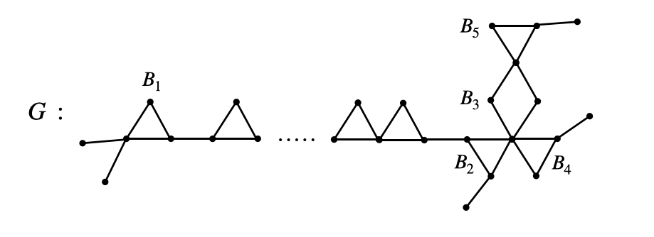
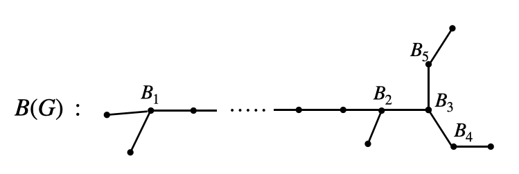
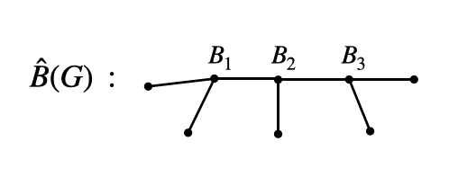
Figure 1: The original graph $G$

Figure 2: A block tree $B(G)$ and the corresponding condensed block tree $\hat{B}(G)$

For any minimal feasible solution $H$ of $k\text{-}\mathrm{FST}$ and a condensed block-tree $\hat{B}(H)$, we refer to the 2NC blocks of $H$ that correspond to internal nodes of $\hat{B}(H)$ as high-degree blocks. The leaves of $\hat{B}(H)$ correspond to the terminals. Edges of $\hat{B}(H)$ correspond to 1-protected paths in $H$ that connect either (i) two high-degree blocks, or (ii) a high-degree block and a terminal, or (iii) two terminals. The end-points of these 1-protected paths are either cut-nodes of $H$ or terminals. Note that some of these 1-protected paths could be trivial paths corresponding to cut-nodes that are common to two high-degree blocks. We now state some useful lemmas that follow from the handshaking lemma applied to $\hat{B}(H)$.

Lemma 9.

The number of internal nodes (i.e., non-leaf nodes) of $\hat{B}(H)$ is at most $k-2$ where $k$ is the number of terminals.

Lemma 10.

The total number of cut-nodes (with repetitions) in high-degree blocks of $H$ is at most $3k-6$ where $k$ is the number of terminals.

Now, we describe our algorithm for unweighted $k\text{-}\mathrm{FST}$. We guess (via enumeration) the high-degree blocks of an optimal solution optsoln corresponding to some condensed block-tree $\hat{B}(\textsc{optsoln})$. The guess would include the number of high-degree blocks and the cut-nodes in each of these high-degree blocks. This is done by picking $3k-6$ nodes of $V$ with replacement and then picking a partition $\widehat{\cal P}$ of these $3k-6$ nodes into at most $k-2$ sets. Let $r\leq k-2$ be the number of sets in the partition $\widehat{\cal P}$. Thus, $\widehat{\cal P}=(X_{1},X_{2},\dots,X_{r})$. For each set $X_{i}$, we use algorithm $\mathcal{A}_{2NC}$ to find $B_{i}$, a minimum size 2NC subgraph of $G$ containing the specified cut-nodes in $X_{i}$, possibly, with some additional Steiner nodes. Finally, we construct a tree that connects these 2NC subgraphs and terminals via 1-protected paths using the following subroutine.

First, for every pair of nodes $(u,v)\in V^{\prime}\times V^{\prime}$, we use algorithm $\mathcal{A}_{\text{2-FST}}$ to find ${G_{uv}^{\min}}$, the minimum size 1-protected path connecting $u$ and $v$ in $G^{\prime}$. We then construct a complete graph $K(X_{1},\ldots,X_{r})$ with $r+k$ nodes that has one node for each set $X_{i}$ and one node corresponding to each terminal $\{t\}$. The cost of an edge between two nodes of $K$ corresponding to node sets $V_{1}$ and $V_{2}$ is given by $\min\{|E({G_{uv}^{\min}})|:u\in V_{1},v\in V_{2}\}$. Note that if there is no 1-protected path connecting a node in $V_{1}$ to a node in $V_{2}$, then we fix the cost of the edge to be infinity. Thus an edge $\bar{e}$ of $K$ corresponds to a subgraph ${G_{\bar{e}}^{\min}}$ in $G^{\prime}$ which is the minimum size 1-protected path whose end points are in $V_{1}$ and $V_{2}$ respectively. We then find a minimum spanning tree $\bar{T}$ in $K$. Note that if $\bar{T}$ has infinite cost, then we output an error. Else, we output the subgraph of $G^{\prime}$ defined by ${G^{\min}}(X_{1},\ldots,X_{r}):=\cup_{\bar{e}\in\bar{T}}{G_{\bar{e}}^{\min}}$.

Algorithm $\mathcal{A}_{\text{k-FST}}(G^{\prime},\;T^{\prime}{,\;\eta})$

(Set parameter) $\eta^{\prime}=\frac{\eta}{k}$;

(Initialize) $H:=G^{\prime}$;

For $S=(v_{1},\ldots,v_{3k-6})\in V^{3k-6}$:

  For $r=1,\ldots,k-2$:

   For partitions $(X_{1},\ldots,X_{r})$ of $S$:

    $\hat{H}:={G^{\min}}(X_{1},\ldots,X_{r})\cup_{i=1}^{r}\mathcal{A}_{2NC}(G,X_{i}{,\;\eta^{\prime}})$;

    Continue the loop if any call to any subroutine reports an error;

    If $|E(\hat{H})|<|E(H)|$, update $H:=\hat{H}$;

   End For;

  End For;

 End For;

Output $H$;

Lemma 11.

Let $H^{*}=(V^{*},E^{*})$ be an optimal subgraph for $k\text{-}\mathrm{FST}$. Assume that each of the calls to the subroutine $\mathcal{A}_{2NC}(G,X_{i},\eta^{\prime})$ returns a valid subgraph ${2NC}(G,X_{i})$ whenever one exists. Let $H=(U,F)$ denote the output of the above algorithm. Then, $H$ is a feasible $k\text{-}\mathrm{FST}$ solution and $|F|\leq|E^{*}|=\textsc{opt}$.

Proof.

We argue that the subgraph $\hat{H}$ in any iteration of the algorithm is a feasible $k\text{-}\mathrm{FST}$ solution. This holds because the algorithm finds 2NC subgraphs ${2NC}(G,X_{i})$ and then connects them to one another and to the terminals using the 1-protected paths in ${G^{\min}}(X_{1},\ldots,X_{r})$. Thus, $T\subseteq V(\hat{H})$ and any unsafe edge $e\in E(\hat{H})$ either lies in a 2NC subgraph of $\hat{H}$ or a 1-protected path in $\hat{H}$, hence, $\hat{H}-e$ is connected.

Now consider a condensed block-tree $\hat{B}(H^{*})$. Let $B^{*}_{1},\ldots,B^{*}_{r^{*}}$ be the high-degree blocks of $H^{*}$ and let $X^{*}_{i}$ be the set of cut-nodes in $B^{*}_{i}$. By Lemma 10, the total number of cut-nodes in all the high-degree blocks $B^{*}_{i}$ is at most $3k-6$. We may assume that it is exactly $3k-6$ by duplicating a cut-node $v\in{X^{*}_{1}}$ multiple times. Consider the iteration of the algorithm where $r=r^{*}$ and $X_{i}=X^{*}_{i}$ for $i=1,\ldots,r^{*}$. Then,

$${|E({2NC}(G,X_{i}))|}\leq|E(B^{*}_{i})|\quad\quad\forall i=1,\ldots,r.$$

Recall that the nodes of $\hat{B}(H^{*})$ correspond to the high-degree blocks $B^{*}_{i}$ (and hence to the node sets $X^{*}_{i}$) or to the terminals $\{t\}$. Also an edge $\bar{e}$ of $\hat{B}(H^{*})$ between nodes corresponding to node sets $V_{1}$ and $V_{2}$ represents a 1-protected path $H^{*}_{\bar{e}}$ in $H^{*}$ whose end-points lie in $V_{1}$ and $V_{2}$ respectively. Hence $\hat{B}(H^{*})$ may be viewed as a subgraph of $K(X_{1},\ldots,X_{r})$. Furthermore, since any two nodes in $H^{*}$ have a 1-protected path between them, $\hat{B}(H^{*})$ must be connected. Finally, by construction of $K$, $|E(H^{*}_{\bar{e}})|\geq c(\bar{e})$ where $c(\bar{e})$ is the cost of the edge $\bar{e}$ in $K$. This implies that the cost of the minimum spanning tree in $K$ is at most $\sum_{\bar{e}\in\hat{B}(H^{*})}|E(H^{*}_{\bar{e}})|$. Hence,

$${|E({G^{\min}}(X_{1},\ldots,X_{r}))|}\leq\sum_{\bar{e}\in\hat{B}(H^{*})}|E(H^{*}_{\bar{e}})|.$$

Combining the two inequalities above we obtain

$${|E(\hat{H})|} =|E({{G^{\min}}(X_{1},\ldots,X_{r})}\cup_{i=1}^{r}{{2NC}(G,X_{i}))}|$$

$$\leq{|E({G^{\min}}(X_{1},\ldots,X_{r}))|}+\sum_{i=1}^{r}{|E({2NC}(G,X_{i}))|}$$

$$\leq\sum_{\bar{e}\in\hat{B}(H^{*})}|E(H^{*}_{\bar{e}})|+\sum_{i=1}^{r}|E(B^{*}_{i})|$$

$$=|E^{*}|$$

The last equation holds because $E^{*}$ partitions into the edge-sets of the high-degree blocks $B^{*}_{i}$ and the edge-sets of the 1-protected paths $H^{*}_{\bar{e}}$. This completes the proof of the lemma. ∎

Theorem 12.

Consider the unweighted $k\text{-}\mathrm{FST}$ problem with $k=O(1)$. Let $\eta>0$ be a parameter. Let $\alpha$ denote the running time of $\mathcal{A}_{\text{2-FST}}$ and let $\beta$ denote the running time of $\mathcal{A}_{\text{2NC}}(\cdot,\cdot,\eta^{\prime})$ with parameter $\eta^{\prime}=\eta/k$. With probability $\geq 1-\eta$, the above randomized algorithm computes an optimal subgraph in time

$${O(n^{2}\alpha\cdot{n^{3k-6}}2^{k}n^{2}\beta\cdot k^{2}\log{k})=O\left(\alpha\cdot\beta\cdot n^{3k}\right)}.$$

Using the running time for $\mathcal{A}_{\text{2NC}}$ given above and the algorithm of [1] for $\mathcal{A}_{\text{2-FST}}$, which has a $n^{O(1)}$ running time, the running time of the above algorithm for $k\text{-}\mathrm{FST}$ is $O\left(n^{O(k)}\cdot\log{\frac{1}{\eta}}\right)$. This leads to the following result for the weighted $k\text{-}\mathrm{FST}$ problem.

Corollary 13.

There is a randomized algorithm for the (weighted) $k\text{-}\mathrm{FST}$ problem that runs in time

$${O\left(n^{O(k)}\cdot\left(\frac{1}{\varepsilon}\right)^{O(k)}\cdot\log{\frac{1}{\eta}}\right)}$$

such that, with probability at least $1-\eta$, the solution returned by the algorithm has cost at most $(1+\varepsilon)$ times the cost of an optimal solution.

Acknowledgements. We are grateful to several colleagues for insightful comments at the start of this project.

References

- [1] David Adjiashvili, Felix Hommelsheim, Moritz Mühlenthaler, and Oliver Schaudt. Fault-tolerant edge-disjoint paths - beyond uniform faults. CoRR, abs/2009.05382, 2020. URL: https://arxiv.org/abs/2009.05382, arXiv:2009.05382.
- [2] Andreas Björklund, Thore Husfeldt, and Nina Taslaman. Shortest cycle through specified elements. In Yuval Rabani, editor, Proceedings of the Twenty-Third Annual ACM-SIAM Symposium on Discrete Algorithms, SODA 2012, Kyoto, Japan, January 17-19, 2012, pages 1747–1753. SIAM, 2012. doi:10.1137/1.9781611973099.139.
- [3] Joseph Cheriyan, Bundit Laekhanukit, Guyslain Naves, and Adrian Vetta. Approximating rooted Steiner networks. ACM Trans. Algorithms, 11(2):8:1–8:22, 2014. doi:10.1145/2650183.
- [4] Nathaniel Dean. Open problems. In Neil Robertson and Paul D. Seymour, editors, Graph Structure Theory, Proceedings of a AMS-IMS-SIAM Joint Summer Research Conference on Graph Minors held June 22 to July 5, 1991, at the University of Washington, Seattle, USA, volume 147 of Contemporary Mathematics, pages 677–688. American Mathematical Society, 1991.
- [5] R. Diestel. Graph Theory (4th ed.). Graduate Texts in Mathematics, Volume 173. Springer-Verlag, Heidelberg, 2010. URL: http://diestel-graph-theory.com/.
- [6] Jon Feldman and Matthias Ruhl. The directed Steiner network problem is tractable for a constant number of terminals. SIAM J. Comput., 36(2):543–561, 2006. doi:10.1137/S0097539704441241.
- [7] Andreas Emil Feldmann, Anish Mukherjee, and Erik Jan van Leeuwen. The parameterized complexity of the survivable network design problem. In Karl Bringmann and Timothy Chan, editors, 5th Symposium on Simplicity in Algorithms, SOSA@SODA 2022, Virtual Conference, January 10-11, 2022, pages 37–56. SIAM, 2022. doi:10.1137/1.9781611977066.4.
- [8] Herbert Fleischner and Gerhard J. Woeginger. Detecting cycles through three fixed vertices in a graph. Inf. Process. Lett., 42(1):29–33, 1992. doi:10.1016/0020-0190(92)90128-I.
- [9] Dorit S. Hochbaum and David B. Shmoys. A unified approach to approximation algorithms for bottleneck problems. J. ACM, 33(3):533–550, 1986. doi:10.1145/5925.5933.
- [10] Oscar H. Ibarra and Chul E. Kim. Fast approximation algorithms for the knapsack and sum of subset problems. J. ACM, 22(4):463–468, 1975. doi:10.1145/321906.321909.
- [11] Tibor Jordán. On minimally -edge-connected graphs and shortest -edge-connected Steiner networks. Discret. Appl. Math., 131(2):421–432, 2003. doi:10.1016/S0166-218X(02)00465-1.
- [12] Alexander Schrijver. Combinatorial Optimization: Polyhedra and Efficiency, volume 24 of Algorithms and Combinatorics. Springer-Verlag Berlin Heidelberg, 2003.
- [13] H. Whitney. Non-separable and planar graphs. Trans. Amer. Math. Soc., 34:339–362, 1932. doi:10.1090/S0002-9947-1932-1501641-2.