sparse-ir: optimal compression and sparse sampling of many-body propagators

Abstract

We introduce sparse-ir, a collection of libraries to efficiently handle imaginary-time propagators, a central object in finite-temperature quantum many-body calculations. We leverage two concepts: firstly, the intermediate representation (IR), an optimal compression of the propagator with robust a-priori error estimates, and secondly, sparse sampling, near-optimal grids in imaginary time and imaginary frequency from which the propagator can be reconstructed and on which diagrammatic equations can be solved. IR and sparse sampling are packaged into stand-alone, easy-to-use Python, Julia and Fortran libraries, which can readily be included into existing software. We also include an extensive set of sample codes showcasing the library for typical many-body and ab initio methods.

Code metadata

Nr.	Code metadata description	Please fill in this column
C1	Current code version	1.0-beta1
C2	Permanent link to code/repository used for this code version	github.com/SpM-lab/sparse-ir; github.com/SpM-lab/SparseIR.jl; github.com/SpM-lab/sparse-ir-fortran
C3	Code Ocean compute capsule	–
C4	Legal Code License	MIT
C5	Code versioning system used	git
C6	Software code languages, tools, and services used	Python or Julia or Fortran
C7	Dependencies	scipy (optional: xprec)
C8	Link to developer documentation/manual	sparse-ir.readthedocs.io; spm-lab.github.io/sparse-ir-tutorial
C9	Support email for questions	github.com/SpM-lab/sparse-ir/issues

1 Motivation and significance

Computational quantum many-body physics is a major driver of advances in materials science, quantum computing, and high-energy physics. Yet, in pushing these fields forward, we face a three-pronged challenge: firstly, the requirement to model more complicated systems in an effort to understand advanced many-body effects, secondly, speeding up the calculations to allow large-scale automatized system discovery, and thirdly, the need for reliable error control to fortify predictive power of the results.

For diagrammatic methods working in imaginary (Euclidean) time—widely used to solve quantum many-body systems—these three prongs translate to the need to compactly store, quickly manipulate, and reliably control the error, respectively, of many-body propagators and the diagrammatic equations in which they appear. Previous efforts either focused on optimizing imaginary time grids [1, 2] or modelling generic smooth functions [3, 4].

The intermediate representation (IR) [5, 6] instead leverages the analytical structure of imaginary-time propagators to construct a maximally compact, orthonormal basis: the number of basis functions needed to represent a propagator scales logarithmically with the desired accuracy and logarithmically with $\Lambda$, the ultraviolet cutoff in units of temperature. (Related approaches either optimize for a different norm [7] or trade some compactness for simpler algorithms [8, 9].) Sparse sampling [10] is a complementary concept which connects the IR to sparse time and frequency grids, which allows us to efficiently move between representations and restrict the solution of diagrammatic equations to those grids. Uniquely, error control is baked into the IR: each basis function comes with an a priori error level, which also means changing accuracy is simply a matter of changing the number of nonzero basis coefficients. The IR for the one-particle basis also serves as a building block for compressing arbitrary $n$-point propagators [11, 12] and fast solutions to the corresponding diagrammatic equations [13].

Precomputed IRs for different cutoffs $\Lambda$ have been released previously as the irbasis library [14]. Using this library, IR and sparse sampling has been successfully employed in numerous physics and chemistry applications  [15, 16, 17, 18, 19, 20, 21, 22, 23, 24, 25, 26, 27, 28].

In the paper, we introduce sparse-ir, a major step forward from the previous library: it computes the basis on the fly, usually within seconds. This not only removes the need for precomputing and shipping databases, it also allows tayloring the cutoff $\Lambda$ and even the type of kernel to the specific application. We also simplify the use of sparse sampling, which previously had to be implemented on top of irbasis by the user. Finally, we improve the infrastructure for two-particle calculations by adding the possibility of augmented and vertex bases [11, 13]. We also provide a set of small, self-contained Jupyter notebooks showcasing the use of IR and sparse sampling for selected physics and quantum chemistry applications, lower the barrier of entry for new users. The library is available as three standalone Python, Julia and Fortran ports, each with minimal dependencies.

The remainder of this paper is organized as follows: after an overview over IR and sparse sampling in Sec. 2, we showcase the use of sparse-ir in a simple Feynman diagrammatic method in Sec. 3. In Sec. 4, we then give an overview of the anatonomy and function of the package. We state our final assessments in Sec. 5.

2 Software description

We are concerned with (retarded) many-body propagators and related functions in equilibrium:

$$G^{\mathrm{R}}(\omega)=-\mathrm{i}\int_{t^{\prime}}^{\infty}\differential{t}\mathrm{e}^{\mathrm{i}\omega t}\langle A(t)B(t^{\prime})\mp B(t^{\prime})A(t)\rangle,$$ (1)

where both $A,B$ are bosonic ($-$) or fermionic ($+$) operators, $\langle\cdot\rangle=\Tr(\mathrm{e}^{-\beta H}\;\cdot\,)/\Tr(\mathrm{e}^{-\beta H})$ is the expectation value, $1/\beta$ is temperature and $H$ is the Hamiltonian. At its core, sparse-ir seeks to (i) maximally compress the information contained in these propagators and (ii) reliably reconstruct this compressed form from sparse time and frequency grids to allow its use in diagrammatic calculations.

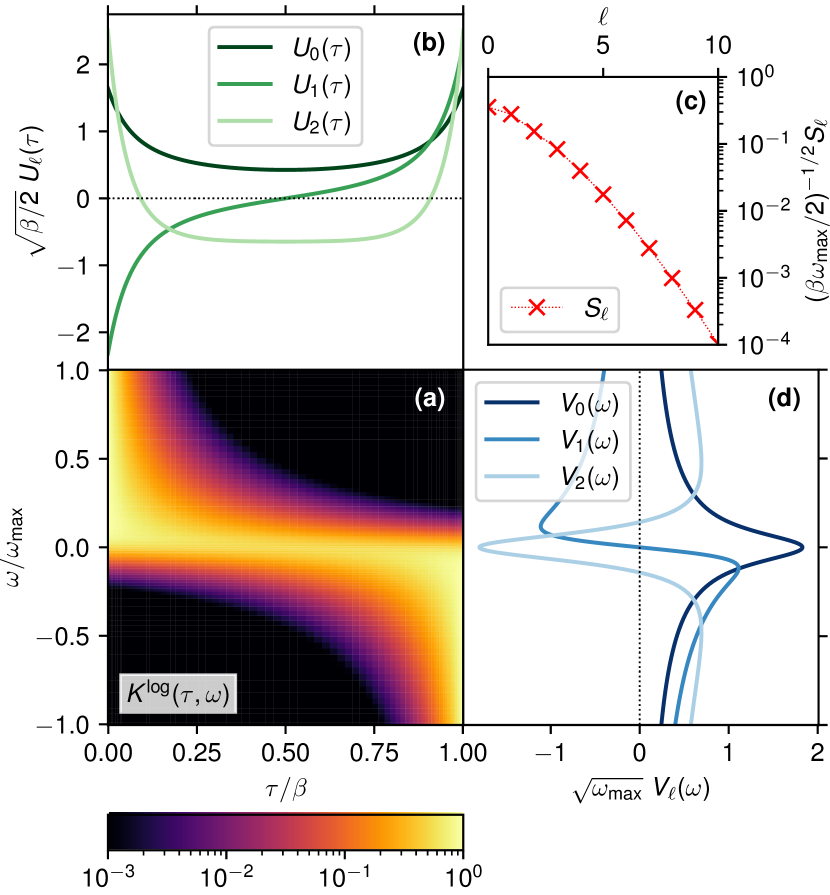
Figure 1: Singular value expansion (4) of the (a) analytic continuation kernel $K$ (3) for $\beta{\omega_{\mathrm{max}}}=30$ into (b) left-singular functions $U_{l}$ on the imaginary-time axis, (c) singular values $S_{l}$, and (d) right-singular functions $V_{l}$ on the real-frequency axis.

To achieve (i) compression, sparse-ir relies on the fact that information is lost in transitioning from the (observable) spectral function $\rho(\omega)=-\frac{1}{\pi}\imaginary G^{\mathrm{R}}(\omega)$ on the real-frequency axis to the propagator $G(\tau)$ on the imaginary-time axis:

$$G(\tau)\equiv-\langle T_{\tau}A(\tau)B(0)\rangle=-\int\differential\omega\;K(\tau,\omega)\,\rho(\omega),$$ (2)

where $K$ is an integral kernel mediating the transition (cf. Sec. 4):

$$K(\tau,\omega)=\frac{\exp(-\tau\omega)}{\exp(-\beta\omega)\pm 1}\Theta({\omega_{\mathrm{max}}}-|\omega|),$$ (3)

$T_{\tau}$ is the time-ordering operator, ${\omega_{\mathrm{max}}}$ is a UV cutoff (upper bound to the bandwidth), and $0<\tau<\beta$ is imaginary time. This information loss is epitomized by the singular value expansion (SVE) [29] of the kernel $K$ [30, 5]:

$$K(\tau,\omega)=\sum_{l=0}^{\infty}U_{l}(\tau)\,S_{l}\,V_{l}(\omega),$$ (4)

where $\{U_{l}\}$ are the left-singular functions, an orthonormal system on the imaginary-time axis, and $\{V_{l}\}$ are the right-singular functions, an orthonormal system on the real-frequency axis. The amount of information retained in the transformation from $V_{l}$ to $U_{l}$ is encoded in the associated (scaled) singular value $S_{l}/S_{0}$. Crucially, $S_{l}$ decays at least exponentially quickly, $\log(S_{l})\sim-l/\log(\beta{\omega_{\mathrm{max}}})$. This information loss on the other hand allows the imaginary-time propagator to be compressed by storing the expansion coefficients of the left-singular functions (“IR basis functions”) $U_{l}$ [6]:

$$G(\tau)=\sum_{l=0}^{L-1}U_{l}(\tau)\,G_{l}+\epsilon_{L}(\tau),$$ (5a)

where $$G_{l}=-S_{l}\int\differential\omega\,V_{l}(\omega)\rho(\omega) \epsilon_{L} \epsilon_{L}\sim S_{L}/S_{0}$$ are the expansion coefficients and is an error term which vanishes exponentially quickly, . Its Fourier transform is given by

$$\hat{G}(\mathrm{i}\omega)=\int_{0}^{\beta}\differential\tau\,\mathrm{e}^{\mathrm{i}\omega\tau}G(\tau)=\sum_{l=0}^{L-1}\hat{U}_{l}(\mathrm{i}\omega)\,G_{l}+\hat{\epsilon}_{L}(\mathrm{i}\omega),$$ (5b)

where $\mathrm{i}\omega=\frac{\mathrm{i}\pi}{\beta}(2n+\zeta)$ is a Matsubara frequency, $\zeta=0$/1 for bosons/fermions, and $\hat{\cdot}$ denotes the Fourier transform. The singular value construction means that the IR basis is (a) optimal in terms of compactness: for, e.g., $\beta{\omega_{\mathrm{max}}}<10^{8}$, no more than 200 coefficients must be stored to obtain full double precision accuracy; (b) orthonormal; and (c) unique, thereby providing a robust and compact storage format.

To achieve (ii) reconstruction, we note that the “polynomial-like” properties of $U_{l}$ [31, 13] guarantee that there exists [32, 33] a sparse set of $\mathcal{O}(L)$ times $\mathcal{T}=\{\tau_{i}\}$ and frequencies $\mathcal{W}=\{\mathrm{i}\omega_{n}\}$ from which we can robustly infer the coefficients [10]. sparse-ir solves the following ordinary least-squares problems:

$$G_{l} =\underset{\{G_{l}\}}{\operatorname{arg\,min}}\sum_{\tau\in\mathcal{T}}\Big{|}G(\tau)-\sum_{l=0}^{L-1}U_{l}(\tau)\,G_{l}\Big{|}^{2},$$ (6a)

$$G_{l} =\underset{\{G_{l}\}}{\operatorname{arg\,min}}\sum_{\mathrm{i}\omega\in\mathcal{W}}\Big{|}\hat{G}(\mathrm{i}\omega)-\sum_{l=0}^{L-1}\hat{U}_{l}(\mathrm{i}\omega)\,G_{l}\Big{|}^{2}.$$ (6b)

Given a sensible choice for the sampling points, Eqs. (5b) and (6) now allow us to move between sparse imaginary-time and frequency grids and compressed representations without any significant loss of precision [10].

3 Example usage

As a simple example, let us perform self-consistent second-order perturbation theory for the single impurity Anderson model at finite temperature. Its Hamiltonian is given by

$$\begin{split}H&=-\mu(\mathrm{c}^{\dagger}_{\uparrow}\mathrm{c}^{\mathchoice{\vphantom{\dagger}}{}{}{}}_{\uparrow}+\mathrm{c}^{\dagger}_{\downarrow}\mathrm{c}^{\mathchoice{\vphantom{\dagger}}{}{}{}}_{\downarrow})+U\mathrm{c}^{\dagger}_{\uparrow}\mathrm{c}^{\dagger}_{\downarrow}\mathrm{c}^{\mathchoice{\vphantom{\dagger}}{}{}{}}_{\downarrow}\mathrm{c}^{\mathchoice{\vphantom{\dagger}}{}{}{}}_{\uparrow}\\ &\hphantom{=}+\sum_{p\sigma}\big{(}V_{p\sigma}\mathrm{f}^{\dagger}_{p\sigma}\mathrm{c}^{\mathchoice{\vphantom{\dagger}}{}{}{}}_{\sigma}+V^{*}_{p\sigma}\mathrm{c}^{\dagger}_{\sigma}\mathrm{f}^{\mathchoice{\vphantom{\dagger}}{}{}{}}_{p\sigma}\big{)}+\sum_{p\sigma}\epsilon_{p}\mathrm{f}^{\dagger}_{p\sigma}\mathrm{f}^{\mathchoice{\vphantom{\dagger}}{}{}{}}_{p\sigma},\end{split}$$ (7)

where $U$ is the electron interaction strength, $\mu$ is the chemical potential, $\mathrm{c}^{\mathchoice{\vphantom{\dagger}}{}{}{}}_{\sigma}$ annihilates an electron on the impurity, $\mathrm{f}^{\mathchoice{\vphantom{\dagger}}{}{}{}}_{p\sigma}$ annihilates an electron in the bath, $\dagger$ denotes the Hermitian conjugate, $p\in\mathbb{R}$ is bath momentum, and $\sigma\in\{\uparrow,\downarrow\}$ is spin. The hybridization strength $V_{p\sigma}$ and bath energies $\epsilon_{p}$ are chosen such that the non-interacting density of states is semi-elliptic with a half-bandwidth of one, $\rho_{0}(\omega)=\frac{2}{\pi}\sqrt{1-\omega^{2}}$, $U=1.2$, $\beta=10$, and the system is half-filled, $\mu=U/2$.

⬇

1import sparse_ir as ir, numpy as np

2basis = ir.FiniteTempBasis(’F’, 10, 8, 1e-6)

3U = 1.2

4def rho0w(w):

5 return np.sqrt(1-w.clip(-1,1)**2) * 2/np.pi

6rho0l = basis.v.overlap(rho0w)

7G0l = -basis.s * rho0l

8Gl_prev = 0

9Gl = G0l

10stau = ir.TauSampling(basis)

11siw = ir.MatsubaraSampling(basis)

12while np.linalg.norm(Gl - Gl_prev) > 1e-6:

13 Gl_prev = Gl

14 Gtau = stau.evaluate(Gl)

15 Sigmatau = U**2 * Gtau**3

16 Sigmal = stau.fit(Sigmatau)

17 Sigmaiw = siw.evaluate(Sigmal)

18 G0iw = siw.evaluate(G0l)

19 Giw = 1/(1/G0iw - Sigmaiw)

20 Gl = siw.fit(Giw)

Figure 2: Self-consistent second-order perturbation theory for a single-impurity Anderson model (7) with a semi-elliptic density of states and $U=1/2$ at half filling and $\beta=10$ using sparse-ir.

We present the associated algorithm in Fig. 2. First, we construct the IR basis for fermions and $\beta=10$, intuit that ${\omega_{\mathrm{max}}}=8$ is larger than the interacting bandwidth and content ourselves with an accuracy of $\epsilon=10^{-6}$ (line 2). We then compute the basis coefficients as $\rho_{0,l}=\int\differential\omega\,V_{l}(\omega)\rho_{0}(\omega)$ (line 6). The non-interacting propagator $G_{0,l}=-S_{l}\rho_{0,l}$ (line 7) serves as initial guess for $G_{l}$ (line 9). We then construct the grids and matrices for sparse sampling (lines 10, 11), after which we enter the self-consistency loop (line 12): At half filling, the second-order self-energy is simply

$$\Sigma(\tau)=U^{2}G^{3}(\tau)$$ (8)

(line 15). We construct this object at the sampling points $\{\tau_{i}\}$ by first expanding $G_{l}$ (line 14). The dynamical part of the self-energy is propagator-like, so it can be modeled by the IR basis (the Hartree and Fock term, if present, needs to be handled separately). The Dyson equation

$$\hat{G}^{-1}(\mathrm{i}\omega)=\hat{G}_{0}^{-1}(\mathrm{i}\omega)-\hat{\Sigma}(\mathrm{i}\omega)$$ (9)

(line 19) is then solved by expanding both $G_{0}$ and $\Sigma$ on the sparse set of frequencies (lines 17, 18). To complete the loop, the IR coefficients for $G$ are then updated (line 20). We converge if the deviation between subsequent iterations (line 13) is consistent with the basis accuracy (line 12).

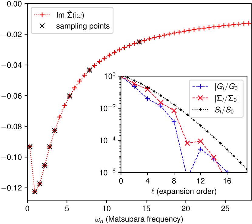
Figure 3: Imaginary part of the Matsubara self-energy $\hat{\Sigma}(\mathrm{i}\omega)$ for the GF(2) calculation in Fig. 2. Black crosses mark the location of sampling points $\mathcal{W}$ on which the Dyson equation (9) is solved and from which the full signal is reconstructed. Inset: normalized IR expansion coefficients of $G$ (plusses) and $\Sigma-\Sigma_{\mathrm{HF}}$ (crosses) and singular values (dots) for comparison. Lines are guides for the eye.

The resulting self-energy $\hat{\Sigma}(\mathrm{i}\omega)$ on the Matsubara axis is presented in Fig. 3 (only the imaginary part is plotted, since the real part is merely a constant $U/2$ at half filling). Instead of a dense mesh (plusses), the Dyson equation has to be solved only on the sampling points (crosses). Since the IR coefficients for both the Green’s function and the self-energy are guaranteed to decay quickly (see inset), this is enough to reconstruct the functions everywhere with the given accuracy bound of $\epsilon=10^{-6}$. We note that this bound and the UV cutoff ${\omega_{\mathrm{max}}}$ are the only discretization parameters we need to supply.

The code in Fig. 2 is short, simple—no explicit Fourier transforms or models are required—yet guarantees the given accuracy goal. Extending the approximation to $\Sigma=GW$ would require only the addition of a bosonic basis, the construction of the RPA diagram, $\Pi(\tau)=G^{2}(\tau)$, and solving the Bethe–Salpeter equation, $\hat{W}(\mathrm{i}\omega)=U+U\hat{\Pi}(\mathrm{i}\omega)\hat{W}(\mathrm{i}\omega)$, where again sparse grids and transformations can be used.

In addition to this example, sparse-ir ships a set of tutorials [34], demonstrating the use of the Python, Julia, and Fortran libraries in typical many-body calculations. Each tutorial contains a short description of the underlying many-body theory as well as sample code utilizing sparse-ir and its expected output. Currently, we include tutorials on: (a) the GF(2) and GW approximation [35, 36], (b) fluctuation exchange (FLEX) [37, 19, 23], (c) the two-particle self-consistent (TPSC) approximation [38, 39], (d) Eliashberg theory for the Holstein–Hubbard model [40, 41, 42, 43], (e) the Lichtenstein formula [44], (f) calculation of the orbital magnetic susceptibility [45, 46, 47, 48, 49, 50, 51, 52], and (g) numerical analytic continuation based on the SpM method [5].

4 Architecture and features

Figure 4: Simplified UML class diagram of the core of sparse-ir. Classes with names in boldface are available from the top namespace.

The main functions of the library are (a) construction and handling of the kernel (3), (b) performing the singular value expansion (4), (c) storage and evaluation of the IR basis functions (5b), and (d) construction of the sampling points and solution of the fitting problem (6). The sparse-ir package was split along these lines into modules, see Fig. 4, which we will briefly describe in the following.

Kernel

Two kernels are packaged with sparse-ir:

$$K^{\mathrm{log}}_{\Lambda}(x,y) =\frac{\exp(-\tfrac{\Lambda}{2}(x+1)y)}{1+\exp(-\Lambda y)}\Theta(1-|y|),$$ (10a)

$$K^{\mathrm{RB}}_{\Lambda}(x,y) =\frac{y\exp(-\tfrac{\Lambda}{2}(x+1)y)}{1-\exp(-\Lambda y)}\Theta(1-|y|).$$ (10b)

Kernels are expressed in terms of dimensionless variables $x$ and $y$ in the interval $[-1,1]$, where $\tau=\frac{\beta}{2}(x+1)$ and $\omega={\omega_{\mathrm{max}}}y$. Instead of parametrization by both inverse temperature $\beta$ and UV cutoff frequency ${\omega_{\mathrm{max}}}$, this allows one to consider only a single scale parameter $\Lambda=\beta{\omega_{\mathrm{max}}}$.

The logistic kernel (10a) is the default kernel used for both fermionic and bosonic propagators for simplicity: even though it is the analytic continuation kernel for fermions, it can also be used to compactly model bosonic propagators [53, 26, 8]. The regularized bosonic kernel (10b) is common in numerical analytic continuation of bosonic functions [54, 55] and is used by the irbasis library for bosonic propagators. Thermal contributions to the susceptibility, $\chi(\omega=0)$, can be modelled by augmenting the basis [13]. User-defined kernels may be added.

Each kernel $K$ can be evaluated by supplying $x,y$, however care must be taken not to lose precision around $x=\pm 1$: in addition to $x$ we use $x_{\pm}\coloneqq 1\pm x$ to full precision to avoid cancellation in the enumerators of Eqs. (10).

Piecewise polynomials

To represent the IR basis functions (4), we employ piecewise Legendre polynomials:

$$P_{nq}(x;\{x_{m}\})\coloneqq\sqrt{\frac{1}{\Delta x_{n}}}P_{q}\!\left(\frac{x-\bar{x}_{n}}{\Delta x_{n}}\right)\Theta(\Delta x_{n}-|x-\bar{x}_{n}|),$$ (11)

where $x_{0}<x_{1}<\cdots<x_{N}$ are the segment edges, $\Delta x_{n}\coloneqq\frac{1}{2}(x_{n}-x_{n-1})$, $\bar{x}_{n}\coloneqq\frac{1}{2}(x_{n}+x_{n-1})$, and $P_{q}$ denotes the $q$-th Legendre polynomial.

Given suitable discretizations of the axes, $\{x_{n}\}$ and $\{y_{n}\}$, as well as a Legendre order $Q$, the left and right IR basis functions can then be expanded as follows:

$$u_{l}(x) \approx\sum_{n=1}^{N}\sum_{q=0}^{Q}u_{lnq}P_{nq}(x;\{x_{0},\ldots,x_{N}\}),$$ (12a)

$$v_{l}(y) \approx\sum_{n^{\prime}=1}^{N^{\prime}}\sum_{q^{\prime}=0}^{Q}v_{ln^{\prime}q^{\prime}}P_{n^{\prime}q^{\prime}}(y;\{y_{0},\ldots,y_{N^{\prime}}\}),$$ (12b)

where $u_{lnq}$ and $v_{ln^{\prime}q^{\prime}}$ are expansion coefficients.

Legendre polynomials have the advantage that their Fourier transform is given analytically [3]:

$$\begin{split}\hat{P}_{nq}(\pm\omega;\{x_{m}\})&\coloneqq\int_{x_{0}}^{x_{N}}\differential{x}\mathrm{e}^{\pm\mathrm{i}\omega x}P_{nq}(x;\{x_{m}\})\\ &=2\sqrt{\Delta x_{n}}\mathrm{e}^{\pm\mathrm{i}\omega\bar{x}_{n}}(\pm\mathrm{i})^{q}j_{q}(\omega\Delta x_{n}),\end{split}$$ (13)

where $\omega\geq 0$ is a frequency and $j_{q}(x)$ is the $q$-th spherical Bessel function. Thus, no numerical integration is necessary, though $\exp(\mathrm{i}\omega x)$ must be analytically mapped back to small $\mathrm{i}\omega x$ to avoid cancellation.

Singular value expansion (SVE)

Given the discretization outlined above, we can relate the SVE (4) needed for constructing the IR basis to the singular value decomposition (SVD) of the following $(NQ)\times(N^{\prime}Q)$ matrix [29, 6]:

$$\begin{split}&A_{nq,n^{\prime}q^{\prime}}=\sqrt{(q+\tfrac{1}{2})(q^{\prime}+\tfrac{1}{2})}\\ &\quad\times\iint\differential{x}\differential{y}P_{nq}(x,\{x_{m}\})P_{n^{\prime}q^{\prime}}(y,\{y_{m}\})K(x,y),\end{split}$$ (14)

where the singular values of $A$ are equal to the singular values $s_{l}$ of the kernel, and the left and right singular vectors are the (scaled) expansion coefficients of $u_{l}(x)$ and $v_{l}(y)$, respectively (12). $L$ is chosen such that $s_{L}<\epsilon s_{0}$, where $\epsilon$ is the desired accuracy of the basis. In practice, we approximate the integral (14) by the associated Gauss–Legendre rule and rewrite the problem as equation for the Gauss nodes [32, 29, 8]. As the kernels (10) are all centrosymmetric, $K(x,y)=K(-x,-y)$, the SVE problem is block-diagonalized for a four-fold speedup [56].

We empirically find that choosing $\{x_{m}\}$ and $\{y_{m}\}$ close to the extrema of the highest-order basis functions, $u_{L-1}(x)$ and $v_{L-1}(y)$, respectively, to provide an excellent discretization, only necessitating $Q=16$ for $\epsilon=10^{-16}$. Since computing the basis functions requires solving the SVE, each kernel maintains approximations to $\{x_{m}\}$ and $\{y_{m}\}$ as hints. As only a fraction $1/Q$ of the singular values of Eq. (14) are needed, we use a truncated SVD algorithm (rank-revealing $QR$ decomposition followed by two-sided Jacobi rotations [57]) at the cost of $\mathcal{O}(N^{\prime 2}NQ^{3})$.

In order to guarantee an accuracy of $\epsilon$ for both singular values and basis functions, one has to compute the SVE with a machine precision of $\epsilon^{2}$ [57]. Thus we compute the SVD in standard double precision for $\epsilon\geq 10^{-8}$ and quadruple precision otherwise. For the latter we have developed the xprec extension to numpy. Note that quadruple precision is only needed in the SVE – the basis functions are stored and evaluated in double precision.

Sampling

The sampling times $\{\tau_{i}\}$ and frequencies $\{\mathrm{i}\omega_{n}\}$ are chosen such that the highest-order basis functions, $U_{L-1}(\tau_{i})$ and $\hat{U}_{L-1}(\mathrm{i}\omega_{n})$, respectively, are locally extremal. To optimize conditioning, $\tau_{1}$ and $\tau_{L}$ are moved from $\pm 1$ to the midpoint of between the $\pm 1$ and the closest root of $U_{L-1}$. Sampling in frequency is conditioned somewhat worse due to the discrete nature of the frequency axis, which is why $\{\mathrm{i}\omega_{n}\}$ are augmented by four additional frequencies.

With the sampling points chosen, sparse sampling now involves transitioning between IR basis coefficients and the value at the sampling points. For evaluation (5b) at the sampling points we multiply with precomputed matrices, $F_{il}\coloneqq U_{l}(\tau_{i})$ and $\hat{F}_{nl}\coloneqq\hat{U}_{l}(\mathrm{i}\omega_{n})$, respectively, at a cost of $\mathcal{O}(L^{2})$. For fitting the IR coefficients, we need to solve the least-squares problems (6). However, multiplying with a precomputed pseudoinverse can lead to loss of backward stability [58], and we observe this in the case of basis augmentation. Instead, we precompute and store the SVD of $F$ and $\hat{F}$ and construct the pseudoinverse on the fly, again at a cost of $\mathcal{O}(L^{2})$.

Julia and Fortran libraries

This software package includes Julia [59] and Fortran [60] libraries. The Julia library implements the full set of functionalities of the Python library with a similar interface. The Fortran library implements only their subset required for its use in ab initio programs: The Fortran library uses the tabulated values of the IR basis functions computed by the Python library. The Fortran interface is fully compatible with the Fortran95 standard and has no additional external dependencies. More detailed descriptions can be found in readme files of the repositories and the tutorials described below.

5 Impact and outlook

We expect that the library will be widely used in many-body and ab initio calculations based on diagrammatic theories such as GW and quantum embedding theories such as the dynamical mean-field theory and its extensions. The computational complexity of diagrammatic calculations based on these technologies grows slower than any power law with respect to the inverse temperature. This makes these technologies particularly efficient and useful in studying systems with a large bandwidth at low temperatures. The library will make new studies for understanding the low-temperature properties of solids and molecules feasible.

To facilitate its application to various fields, the library supports languages popular in many different areas (Python and Julia for prototyping, Fortran, C, and C++ for existing ab-initio codes.) The library is shipped with many self-contained tutorials on specific topics in different fields of physics.

6 Conclusions

We present intermediate representation (IR) and sparse sampling for efficient many-body and ab initio calculations based on imaginary-time propagators. These methods are implemented in Python/Julia/Fortran libraries to allow researchers in a large community of many-body physics and ab initio calculations to use them.

Conflict of interest

We wish to confirm that there are no known conflicts of interest associated with this publication and there has been no significant financial support for this work that could have influenced its outcome.

References

- [1] W. Ku, A. G. Eguiluz, Band-gap problem in semiconductors revisited: Effects of core states and many-body self-consistency, Phys. Rev. Lett. 89 (2002) 126401. doi:10.1103/PhysRevLett.89.126401.
- [2] A. A. Kananenka, J. J. Phillips, D. Zgid, Efficient temperature-dependent Green’s functions methods for realistic systems: Compact grids for orthogonal polynomial transforms, J. Chem. Theory Comput. 12 (2) (2016) 564–571. doi:10.1021/acs.jctc.5b00884.
- [3] L. Boehnke, H. Hafermann, M. Ferrero, F. Lechermann, O. Parcollet, Orthogonal polynomial representation of imaginary-time Green’s functions, Phys. Rev. B 84 (2011) 075145. doi:10.1103/PhysRevB.84.075145.
- [4] X. Dong, D. Zgid, E. Gull, H. U. R. Strand, Legendre-spectral Dyson equation solver with super-exponential convergence, J. Chem. Phys. 152 (13) (2020) 134107. doi:10.1063/5.0003145.
- [5] J. Otsuki, M. Ohzeki, H. Shinaoka, K. Yoshimi, Sparse modeling approach to analytical continuation of imaginary-time quantum Monte Carlo data, Phys. Rev. E 95 (2017) 061302. doi:10.1103/PhysRevE.95.061302.
- [6] H. Shinaoka, J. Otsuki, M. Ohzeki, K. Yoshimi, Compressing Green’s function using intermediate representation between imaginary-time and real-frequency domains, Phys. Rev. B 96 (3) (2017) 35147. doi:10.1103/PhysRevB.96.035147.
- [7] M. Kaltak, G. Kresse, Minimax isometry method: A compressive sensing approach for Matsubara summation in many-body perturbation theory, Phys. Rev. B 101 (2020) 205145. doi:10.1103/PhysRevB.101.205145.
- [8] J. Kaye, K. Chen, O. Parcollet, Discrete Lehmann representation of imaginary time Green’s functions, arXiv (2021). arXiv:2107.13094.
- [9] J. Kaye, K. Chen, H. U. R. Strand, libdlr: Efficient imaginary time calculations using the discrete Lehmann representation, arXiv (2021). arXiv:2110.06765.
- [10] J. Li, M. Wallerberger, N. Chikano, C.-N. Yeh, E. Gull, H. Shinaoka, Sparse sampling approach to efficient ab initio calculations at finite temperature, Phys. Rev. B 101 (3) (2020) 035144. doi:10.1103/physrevb.101.035144.
- [11] H. Shinaoka, J. Otsuki, K. Haule, M. Wallerberger, E. Gull, K. Yoshimi, M. Ohzeki, Overcomplete compact representation of two-particle Green’s functions, Phys. Rev. B 97 (2018) 205111. doi:10.1103/PhysRevB.97.205111.
- [12] H. Shinaoka, D. Geffroy, M. Wallerberger, J. Otsuki, K. Yoshimi, E. Gull, J. Kuneš, Sparse sampling and tensor network representation of two-particle Green’s functions, SciPost Phys. 8 (2020) 12. doi:10.21468/SciPostPhys.8.1.012.
- [13] M. Wallerberger, H. Shinaoka, A. Kauch, Solving the Bethe–Salpeter equation with exponential convergence, Phys. Rev. Research 3 (2021) 033168. doi:10.1103/PhysRevResearch.3.033168.
- [14] N. Chikano, K. Yoshimi, J. Otsuki, H. Shinaoka, irbasis: Open-source database and software for intermediate-representation basis functions of imaginary-time Green’s function, Comput. Phys. Commun. 240 (2019) 181–188. doi:10.1016/j.cpc.2019.02.006.
- [15] T. Nomoto, T. Koretsune, R. Arita, Local force method for the ab initio tight-binding model: Effect of spin-dependent hopping on exchange interactions, Phys. Rev. B 102 (1) (2020) 014444. doi:10.1103/physrevb.102.014444.
- [16] T. Nomoto, T. Koretsune, R. Arita, Formation mechanism of the helical Q structure in Gd-based skyrmion materials, Phys. Rev. Lett. 125 (11) (2020) 117204. doi:10.1103/physrevlett.125.117204.
- [17] Y. Nomura, T. Nomoto, M. Hirayama, R. Arita, Magnetic exchange coupling in cuprate-analog d9 nickelates, Phys. Rev. Research 2 (4) (2020) 043144. doi:10.1103/physrevresearch.2.043144.
- [18] S. Iskakov, C.-N. Yeh, E. Gull, D. Zgid, Ab initio self-energy embedding for the photoemission spectra of NiO and MnO, Phys. Rev. B 102 (8) (2020) 085105. doi:10.1103/physrevb.102.085105.
- [19] N. Witt, E. G. C. P. van Loon, T. Nomoto, R. Arita, T. O. Wehling, Efficient fluctuation-exchange approach to low-temperature spin fluctuations and superconductivity: From the Hubbard model to , Phys. Rev. B 103 (2021) 205148. doi:10.1103/PhysRevB.103.205148.
- [20] P. Pokhilko, S. Iskakov, C.-N. Yeh, D. Zgid, Evaluation of two-particle properties within finite-temperature self-consistent one-particle green’s function methods: Theory and application to GW and GF2, J. Chem. Phys. 155 (2) (2021) 024119. doi:10.1063/5.0054661.
- [21] C.-N. Yeh, S. Iskakov, D. Zgid, E. Gull, Electron correlations in the cubic paramagnetic perovskite : Results from fully self-consistent self-energy embedding calculations, Phys. Rev. B Condens. Matter 103 (19) (May 2021). doi:10.1103/PhysRevB.103.195149.
- [22] C.-N. Yeh, A. Shee, Q. Sun, E. Gull, D. Zgid, Relativistic self-consistent : Exact two-component formalism with one-electron approximation for solids, arXiv (2022). arXiv:2202.02252.
- [23] N. Witt, J. M. Pizarro, J. Berges, T. Nomoto, R. Arita, T. O. Wehling, Doping fingerprints of spin and lattice fluctuations in moiré superlattice systems, Phys. Rev. B 105 (2022) L241109. doi:10.1103/PhysRevB.105.L241109.
- [24] Y. Nagai, H. Shinaoka, Smooth self-energy in the exact-diagonalization-based dynamical mean-field theory: Intermediate-representation filtering approach, J. Phys. Soc. Japan 88 (6) (2019) 064004. doi:10.7566/jpsj.88.064004.
- [25] Y. Nagai, Intrinsic vortex pinning in superconducting quasicrystals, arXiv (2021). arXiv:2111.13288.
- [26] Y. N. Etsuko Itou, QCD viscosity by combining the gradient flow and sparse modeling methods, arXiv (2021). arXiv:2110.13417.
- [27] R. Sakurai, W. Mizukami, H. Shinaoka, Hybrid quantum-classical algorithm for computing imaginary-time correlation functions, arXiv (2021). arXiv:2112.02764.
- [28] Y. Nagai, H. Shinaoka, Sparse modeling approach for quasiclassical theory of superconductivity, arXiv (2022). arXiv:2205.14800.
- [29] P. C. Hansen, Discrete Inverse Problems: Insights and Algorithms, SIAM, 2010. doi:10.1137/1.9780898718836.
- [30] R. K. Bryan, Maximum entropy analysis of oversampled data problems, Eur. Biophys. J. 18 (1990) 165–174. doi:10.1007/BF02427376.
- [31] S. Karlin, Total Positivity, Stanford University Press, 1968.
- [32] V. Rokhlin, N. Yarvin, Generalized Gaussian quadratures and singular value decompositions of integral operators, SIAM J. Sci. Comput. 20 (1996) 44. doi:10.1137/S1064827596310779.
- [33] H. Shinaoka, N. Chikano, E. Gull, J. Li, T. Nomoto, J. Otsuki, M. Wallerberger, T. Wang, K. Yoshimi, Efficient ab initio many-body calculations based on sparse modeling of Matsubara Green’s function, arXiv (2021). arXiv:2106.12685.
- [34] https://spm-lab.github.io/sparse-ir-tutorial (2022).
- [35] L. Hedin, New method for calculating the one-particle Green’s function with application to the electron-gas problem, Phys. Rev. 139 (1965) A796–A823. doi:10.1103/PhysRev.139.A796.
- [36] F. Aryasetiawan, O. Gunnarsson, The GW method, Rep. Prog. Phys. 61 (3) (1998) 237–312. doi:10.1088/0034-4885/61/3/002.
- [37] N. E. Bickers, D. J. Scalapino, S. R. White, Conserving approximations for strongly correlated electron systems: Bethe–Salpeter equation and dynamics for the two-dimensional Hubbard model, Phys. Rev. Lett. 62 (1989) 961–964. doi:10.1103/PhysRevLett.62.961.
- [38] Y. M. Vilk, A.-M. S. Tremblay, Non-perturbative many-body approach to the Hubbard model and single-particle pseudogap, Journal de Physique I 7 (11) (1997) 1309–1368. doi:10.1051/jp1:1997135.
- [39] A.-M. S. Tremblay, Two-particle-self-consistent approach for the Hubbard model, in: A. Avella, F. Mancini (Eds.), Strongly Correlated Systems: Theoretical Methods, Springer Berlin Heidelberg, Berlin, Heidelberg, 2012, pp. 409–453. doi:10.1007/978-3-642-21831-6_13.
- [40] G. M. Eliashberg, Interactions between electrons and lattice vibrations in a superconductor, Soviet Phys. JETP 11 (1960) 696.
- [41] D. J. Scalapino, The electron-phonon interaction and strong-coupling superconductors, in: R. D. Parks (Ed.), Superconductivity, 1st Edition, CRC Press, Boca Raton, FL, 1969, p. 112. doi:10.1201/9780203737965.
- [42] J. Zhong, H.-B. Schüttler, Polaronic anharmonicity in the Holstein–Hubbard model, Phys. Rev. Lett. 69 (1992) 1600–1603. doi:10.1103/PhysRevLett.69.1600.
-
[43]
Y. Kaga, P. Werner, S. Hoshino,
Eliashberg theory
of the Jahn-Teller-Hubbard model, Phys. Rev. B 105 (2022) 214516.
doi:10.1103/PhysRevB.105.214516.
URL https://link.aps.org/doi/10.1103/PhysRevB.105.214516 - [44] A. I. Lichtenstein, M. I. Katsnelson, V. A. Gubanov, Exchange interactions and spin-wave stiffness in ferromagnetic metals, J. Phys. F: Metal Phys. 14 (7) (1984) L125–L128. doi:10.1088/0305-4608/14/7/007.
- [45] H. Fukuyama, Theory of orbital magnetism of Bloch electrons: Coulomb interactions, Progress of Theoretical Physics 45 (3) (1971) 704–729. doi:10.1143/PTP.45.704.
- [46] G. Gómez-Santos, T. Stauber, Measurable lattice effects on the charge and magnetic response in graphene, Phys. Rev. Lett. 106 (2011) 045504. doi:10.1103/PhysRevLett.106.045504.
- [47] A. Raoux, F. Piéchon, J.-N. Fuchs, G. Montambaux, Orbital magnetism in coupled-bands models, Phys. Rev. B 91 (2015) 085120. doi:10.1103/PhysRevB.91.085120.
- [48] F. Piéchon, A. Raoux, J.-N. Fuchs, G. Montambaux, Geometric orbital susceptibility: Quantum metric without Berry curvature, Phys. Rev. B 94 (2016) 134423. doi:10.1103/PhysRevB.94.134423.
- [49] M. Ogata, H. Fukuyama, Orbital magnetism of Bloch electrons: I. General formula, J. Phys. Soc. Japan 84 (12) (2015) 124708. doi:10.7566/JPSJ.84.124708.
- [50] H. Matsuura, M. Ogata, Theory of orbital susceptibility in the tight-binding model: Corrections to the Peierls phase, J. Phys. Soc. Japan 85 (7) (2016) 074709. doi:10.7566/JPSJ.85.074709.
- [51] M. Ogata, Orbital magnetism of Bloch electrons: II. Application to single-band models and corrections to landau–peierls susceptibility, J. Phys. Soc. Japan 85 (6) (2016) 064709. doi:10.7566/JPSJ.85.064709.
- [52] M. Ogata, Orbital magnetism of Bloch electrons: III. Application to graphene, J. Phys. Soc. Japan 85 (10) (2016) 104708. doi:10.7566/JPSJ.85.104708.
- [53] H. B. Meyer, Calculation of the shear viscosity in gluodynamics, Phys. Rev. D 76 (2007) 101701. doi:10.1103/PhysRevD.76.101701.
- [54] M. Jarrell, J. Gubernatis, Bayesian inference and the analytic continuation of imaginary-time quantum Monte Carlo data, Phys. Rep. 269 (3) (1996) 133–195. doi:10.1016/0370-1573(95)00074-7.
- [55] Y. Motoyama, K. Yoshimi, J. Otsuki, Robust analytic continuation combining the advantages of the sparse modeling approach and the Padé approximation, Phys. Rev. B 105 (2022) 035139. doi:10.1103/PhysRevB.105.035139.
- [56] N. Chikano, J. Otsuki, H. Shinaoka, Performance analysis of a physically constructed orthogonal representation of imaginary-time Green’s function, Phys. Rev. B 98 (3) (2018) 035104. doi:10.1103/PhysRevB.98.035104.
- [57] G. H. Golub, C. F. van Loan, Matrix Computations, 3rd Edition, Johns Hopkins University Press, 1996.
- [58] J. H. Wilkinson, Rounding Errors in Algebraic Processes, Prentice–Hall, 1963.
- [59] https://github.com/SpM-lab/SparseIR.jl (2022).
- [60] https://github.com/SpM-lab/sparse-ir-fortran (2022).