Effects of dipolar coupling on an entanglement storage device

Abstract

Quantum computation requires efficient long-term storage devices to preserve quantum states. An attractive candidate for such storage devices is qubits connected to a common dissipative environment. The common environment gives rise to persistent entanglements in these qubit systems. Hence these systems act efficiently as a storage device of entanglement. However, the existence of a common environment often requires the physical proximity of the qubits and hence results in direct dipolar coupling between the qubits. In this work, we investigate effects of the secular and the nonsecular part of the dipolar coupling on the environment-induced entanglement using a recently-proposed fluctuation-regulated quantum master equation [A. Chakrabarti and R. Bhattacharyya, Phys. Rev. A 97, 063837 (2018)]. We show that nonsecular part of the dipolar coupling results in reduced entanglement and hence less efficiency of the storage devices. We also discuss the properties of efficient storage that mitigates the detrimental effects of the dipolar coupling on the stored entanglement.

I Introduction

In quantum information processing, the generation and the preservation of entanglements are particularly important operations. The preservation or storage of entanglements is challenging since all quantum systems are, to some extent, coupled to their environments. The dissipation originating from the environment destroys the coherence and entanglement in quantum systems. Naturally, a method of storage that takes into account the environment’s dissipative nature and yet provides a long-lived entangled state is highly desired.

One of the earliest clues to solve this problem was found when two decades ago, Cabrillo and others and Plenio and others separately reported the generation of spatially separated entangled atoms Cabrillo et al. (1999); Plenio et al. (1999); Beige et al. (2000). While Cabrillo and others created the entanglement by simultaneous excitation of the atoms, Plenio and others used a leaky cavity to couple the atoms. In this sense, the later work is possibly the first use of a dissipative environment to generate entanglement in spatially distant atoms. At the same time, Arnesen and others investigated the entanglement in a Heisenberg 1D spin-chain, where the coupling gives rise to the entanglement but not in the presence of a heat bath Arnesen et al. (2001). Within a few months, several groups reported that a common dissipative environment gives rise to entangled quantum systems Schneider and Milburn (2002); Kim et al. (2002); Basharov (2002); Jakóbczyk (2003). Subsequently, Braun showed that the generation of the entangled states may not require a direct coupling between the quantum systems and can persist for arbitrarily long times Braun (2002). Later, Benatti and others demonstrated in a series of works that Markovian quantum master equations (QME) could be used to arrive at the persistent bath-induced entanglements Benatti et al. (2003); Benatti and Floreanini (2004, 2006a, 2006b). They have also found that the final entangled state might depend on the initial value of the entanglement Benatti and Floreanini (2006a); Choi and Lee (2007). Later a complete characterization of the entangled phase for a pair of resonant oscillators connected to a common bath was provided by Paz and others Paz and Roncaglia (2008). In the remaining parts of the manuscript, we shall refer to this type of entanglement as the environment-induced entanglement (EIE).

When a pair of qubits are coupled to a single common dissipative environment, one of the eigenstates of the Lindbladian is the singlet state density matrix. Naturally, a pair of qubits prepared in this state will remain unaffected by the dissipator. This remains the basic working principle of the entanglement storage solution based on a bipartite system in the common environment. However, the particular form of the dissipator from the common environment is strongly sensitive to the distance between the qubits. In an important work, Zell and others showed that the entanglement generated by a heat bath is persistent only if the distance between the quantum systems is small compared to the cutoff wavelength of the system-bath interaction Zell et al. (2009). The physical proximity of the qubits indicates that the qubits could be dipolar coupled.

The works of Zell, McCutcheon, and Jeske showed that the distance between the non-interacting qubit pair must be small to have a persistent entanglement; otherwise, the entanglement decays exponentially with the increasing distance between the qubits Zell et al. (2009); McCutcheon et al. (2009); Jeske and Cole (2013). The analysis relies on the fact that the bath correlation decreases exponentially with a characteristic length scale for a simple bosonic bath. In general, one should also include a qubit pair’s direct dipolar interaction and system-environment coupling in the dynamics. After all, if one restricts the distance between the qubit pair to keep those within the bath-correlation length, it is expected that a dipolar interaction between this qubit pair would have a measurable effect. To keep track of various terms appearing in the dipolar interaction, following standard practice, we divide them into secular and nonsecular parts, where the former commutes with the Zeeman part of the qubit Hamiltonians Duer (2001).

An important aspect of the dipolar coupling between the qubits is the contribution from the nonsecular part of the dipolar Hamiltonians. We have shown recently that such terms significantly influence the lifetime of coherences in the case of a time-periodic Hamiltonian Saha and Bhattacharyya (2022). Moreover, the seminal works of Bloembergen and others established long ago that the nonsecular parts of the dipolar interactions contributed to the transition probabilities Bloembergen et al. (1948). Therefore, such terms should be included in analyzing two or higher qubit networks. Now despite having a very large volume of literature on this problem, the effect of the dipolar coupling on persistent entanglements has not hitherto been investigated. So, in this work, we specifically seek an answer to the following question: in the context of a dipolar coupled qubit pair in a spatially-correlated and fluctuating environment, how does the dipolar interaction affect the persistent entanglement? A particularly important aspect of this question is whether the higher-order effects of the dipolar coupling play a role in these dynamics. We note that one needs an appropriate quantum master equation to include the aforementioned effects in the equations of motion of the dipolar systems.

In the traditional form of the quantum master equation, the system-environment coupling provides the dissipator, and other interactions, such as the drive or the dipolar interactions, contribute to the first-order processes. The fluctuation-regulated quantum master equation shows that other interactions, can have a Redfield-like second-order effect in the dynamics in addition to the dissipator from the system-environment coupling Chakrabarti and Bhattacharyya (2018a). The dissipator from the drive, which provides a non-Bloch decay, has also been verified by Chakrabarti and others Chakrabarti and Bhattacharyya (2018b). Later, Chanda and others have shown that this drive-induced dissipation from FRQME results in an optimal condition of the quantum gates Chanda and Bhattacharyya (2020). Moreover, Chatterjee and others have recently demonstrated that the FRQME could successfully explain the frequency-dependent non-linear behavior of the light shifts and Bloch-Siegert shifts Chatterjee and Bhattacharyya (2020). Recently, we have studied how such effects give rise to the decoherences in a dipolar coupled systems Saha and Bhattacharyya (2022).

So, in this manuscript, we systematically study the effect of these terms on quantum storage solutions. We shall show that a direct dipolar coupling reduces the magnitude of the stored entanglement.

We organize the manuscript in the following order. The description of the system consisting of dipolar coupled qubits, weakly interacting with a spatially correlated bosonic bath is given in section II. The dynamical equation for the system using FRQME is introduced in terms of symmetric and anti-symmetric observables in section III. The dynamical behaviors and the steady-state solutions which have been analyzed for different parameter values, are described in section IV. In the same section, we also demonstrate the generation of the entanglement and their dependence on the dipolar interactions. Finally, we discuss the results, and their implications on the EIE-based storage devices in section V. In appendix A, we provide a brief sketch of the derivation of the recently-proposed FRQME. The complete set of the dynamical equations, including the dipolar coupling and a spatially correlated environment is given in appendix B.

II The model

As a specific realization of a qubit, we choose a spin-1/2 particle placed in a static homogeneous magnetic field. We consider two such particles coupled to an environment that is in thermal equilibrium at an inverse temperature $\beta$. We assume that the spins are dipolar coupled whose strength scales as $1/r^{3}$, where $r$ is assumed to be the distance between the two qubits Duer (2001).

The full Hamiltonian of the system and the environment can be written as,

$$\mathcal{H}=\mathcal{H}_{1}^{\circ}+\mathcal{H}_{2}^{\circ}+\mathcal{H}_{L}^{\circ}+\mathcal{H}_{\text{\tiny SL}}+\mathcal{H}_{\text{\tiny DD}}+H_{\text{\tiny L}}(t),$$ (1)

where,$\mathcal{H}_{n}^{\circ}=\frac{\omega_{\circ}}{2}\sigma_{z}^{n}$ is the Zeeman Hamiltonian of the $n^{\rm th}$ qubit, $\sigma_{\alpha},\alpha\in{x,y,z}$ are Pauli matrices for spin-1/2, and $\omega_{\circ}$ is the Larmor frequency. For simplicity, we assumed that the Larmor frequencies of the two spins are identical. $\mathcal{H}_{L}^{\circ}$ is the free Hamiltonian of the environment and can be modeled as a large collection of harmonic oscillators which mimics a spatially correlated bosonic bath, to which the spins are coupled.

The construction of the system-environment coupling is largely motivated by the works of McCutcheon and others and Jeske and others . Following their works, we write the Hamiltonian of system-environment coupling as $\mathcal{H}_{\text{\tiny SL}}=\sum\limits^{2}_{n=1}(\sigma_{+}^{n}\mathcal{L}_{-}B(t)\eta(\vec{r}_{n})+\sigma_{-}^{n}\mathcal{L}_{+}B^{\star}(t)\eta^{\star}(\vec{r}_{n}))$ where, $B(t)$ is the system-environment coupling strength between the spin and the environment, $\eta(\vec{r}_{n})$ is the spatial part of the field due to the environment at the position of $n^{\rm th}$ spin, $\sigma_{\pm}^{n}$ are the raising and the lowering operators for $n^{\rm th}$ spin, $\mathcal{L}_{+}$ and $\mathcal{L}_{-}$ are the raising and the lowering operators of the enviroment, which, for simplicity, are assumed to be resonant with the qubit pair. The correlation between the $\eta(\vec{r})$ decides the nature of the environment. One may choose a suitable correlation to render the environment to be local or common, as discussed in more detail in the next section.

The dipolar interaction can also be conveniently written using the irreducible spherical tensors as

$$\mathcal{H}_{\text{\tiny DD}}=\omega_{d}\sum\limits_{m=-2}^{2}(-1)^{m}Y_{-m}^{2}(\theta,\phi)T_{m}^{2}=\sum\limits_{m=-2}^{2}\omega_{d,m}T_{m}^{2},$$ (2)

where, $Y_{-m}^{2}(\theta,\phi)$ is the spherical harmonics of rank $2$ and order $-m$, $T_{m}^{2}$ is the irreducible spherical tensor of rank $2$ and order $m$, and $\omega_{d,m}=(-1)^{m}Y_{-m}^{2}(\theta,\phi)\omega_{d}$ is an abbreviated form introduced for notional simplicity. $\theta$ and $\phi$ are the polar and azimuthal angle of the orientation of the dipolar vector w.r.t. the direction of the polarization of the spins, respectively Smith et al. (1992a, b). We also have $\omega_{d}=\sqrt{\frac{6\pi}{5}}\frac{\gamma^{2}\hbar}{r^{3}}$, where $\gamma$ is the gyromagnetic ratio of the spin and $r$ is the distance between the spins.

We must note that the assumption of a complete dipolar interaction between the qubits, as given above, instead of a simplified $\vec{\sigma}^{1}.\vec{\sigma}^{2}$ secular form results in certain differences in the dynamics of the qubits. First of all, the secular form (contains only the $T_{0}^{2}$ term) is a part of the full form given above. In the interaction representation, $m\neq 0$ terms are the time-dependent part of dipolar coupling. These terms contribute to the dissipator and result in the reduction of the persistent entanglement of the qubit pairs. Other differences which results from $T_{m}^{2}\ \forall\ m\neq 0$ would be discussed in detail in the section III.

Finally, $H_{\text{\tiny L}}(t)$ denotes time-dependent thermal fluctuations acting on the environment. Since the thermal fluctuations are ubiquitous in an environment, we explicitly take this into account along with the other terms in the Hamiltonian. Since the thermal fluctuations do not destroy the equilibrium of the environment, as a simple model, we assume that $H_{\text{\tiny L}}(t)$ commutes with the static Hamiltonian of the environment $\mathcal{H}^{\circ}_{L}$. It is also assumed that the timescale of fluctuations is much faster than the timescale of the system. The explicit form of the fluctuation Hamiltonian is given by

$$\mathcal{H}_{\text{\tiny L}}(t)=\sum_{i}f_{i}(t)|\phi_{i}\rangle\langle\phi_{i}|$$ (3)

where $\{|\phi_{i}\rangle\}$ are the eigenstates of $\mathcal{H}_{L}^{\circ},$ $i$ is the number of energy levels of the environment. Here, $f_{i}$ is modeled as the stationary and delta-correlated, Gaussian stochastic variables with standard deviation $K$. Therefore, $\overline{f_{i}(t)}=0$, $\overline{f_{i}(t_{a})f_{j}(t_{b})}=\frac{1}{\tau_{c}}\delta_{ij}\delta(t_{a}-t_{b})$ and $K^{2}/2=1/\tau_{c}$.

III Equations of motion

To arrive at the equation of motion from the above Hamiltonian, we use recently-introduced fluctuation-regulated quantum master equation, whose form is given by,

$$\frac{d\rho_{s}}{dt} = -i\,\text{Tr}_{L}\Big{[}H_{\text{\tiny eff}}(t),\rho_{s}(t)\otimes\rho_{L}^{eq}\Big{]}^{sec}$$ (4)

$$-\int\limits^{\infty}_{0}d\tau\,\text{Tr}_{L}\Big{[}H_{\text{\tiny eff}}(t),\Big{[}H_{\text{\tiny eff}}(t-\tau),\rho_{s}(t)\otimes\rho_{L}^{eq}\Big{]}\Big{]}^{sec}e^{-\frac{|\tau|}{\tau_{c}}}$$

where, $H_{\text{\tiny eff}}$ contains the system-environment coupling and other interactions. We note that the effect of the fluctuations are contained in the kernel $e^{-\frac{|\tau|}{\tau_{c}}}$ which is obtained from a cumulant expansion of the propagator containing the fluctuations. The equation is written in the interaction representation w.r.t. to the static Hamiltonians of the system and the environment. Since, FRQME is relatively new, hence we provide a brief summary of its derivation in the appendix A.

We note that the spectral density functions of the system-environment coupling are obtained as

$$\int\limits_{0}^{\infty}d\tau e^{-\tau/\tau_{c}}\langle B_{\rm int}(t)B_{\rm int}^{\star}(t-\tau)\rangle\text{Tr}_{\text{L}}\{\mathcal{L}_{\pm}\mathcal{L}_{\mp}\rho_{L}^{eq}\}\langle\eta(\vec{r}_{n})\eta^{\star}(\vec{r}_{m})\rangle$$ (5)

where, $B_{\rm int}(t)$ is the time-dependent scalar part of the system-environment coupling in the interaction representation and we write the Fourier transform of the time correlation $\langle B_{\rm int}(t)B_{\rm int}^{\star}(t-\tau)\rangle=J\pm i\delta\omega$, with $J$ and $\delta\omega$ denoting the real and the imaginary parts. The term $\langle\eta(\vec{r}_{n})\eta(\vec{r}_{m})\rangle=\alpha^{(1-\delta_{nm})}$ indicates the spatial correlation of the bath, We note that the scalar factor $\alpha\in[0,1]$ appears only in the cross terms, when the environment couples two different spins ($n\neq m$) through the environment operator. For the operator part, we assume that $\text{Tr}_{\text{L}}\{\mathcal{L}_{\pm}\mathcal{L}{\mp}\rho_{L}^{eq}\}=1\pm M_{\circ}$ where $\rho_{L}^{eq}$ is the equilibrium density matrix of the environment. This assumption implies that the qubits will inherit equilibrium populations $(1\pm M_{\circ})/2$, i.e., an equilibrium polarization $\langle\frac{\sigma_{z}}{2}\rangle=M_{\circ}$ when the environment is completely local, i.e., $\alpha=0.$ We note again that in the above, it is also assumed that only energy levels of the environment contribute to the above integral whose separation exactly matches with the Larmor frequency of qubits i.e. the resonant modes.

A common environment could be modeled as a tight-binding chain of oscillators to which the qubits are coupled. For such cases, $\alpha$ had been shown to be a decreasing function of the distance between the qubits $r$. It could be chosen to have an exponential form $\alpha=\exp(-r/\xi)$, where $\xi$ is the correlation length of the spatially correlated environment originating from the chain of oscillators Jeske and Cole (2013). In such a formulation, $\alpha$ remains a measure of the commonness of the environment. We refer to the works of McCutcheon and others for more details on the spatially correlated environment McCutcheon et al. (2009).

We note that $\alpha=0$ signifies a separate local environment for each qubit. With $\alpha=0,$ the qubits relax to their equilibrium polarization with a time constant of $1/J.$ The $\delta\omega$ terms in the spectral density give rise to the Lamb shifts in equations of the observables that do not commute with $\sigma_{z}^{(1,2)}$. On the other hand, $\alpha=1$ indicates that both the spins are coupled to a single common environment. For intermediate values of $\alpha$, the environment is a mixture of the common and the local environments. Interestingly, since $\alpha$ and the dipolar coupling both are functions of $r$, we expect competition between the two distance-dependent processes and investigate that in this manuscript.

Using FRQME, we obtain the dynamical equation as,

$$\frac{d\rho_{s}}{dt} = -i\big{[}\omega_{d,0}T^{2}_{0}+H_{\rm Lamb}+H_{\rm dds},\rho_{s}\big{]}+\mathcal{D}\rho_{s}+\mathcal{Q}\rho_{s}$$ (6)

where, $H_{\rm Lamb}$ is the Lamb shift from the system-environment coupling, and is given by,

$$H_{\rm Lamb} = -\sum\limits_{i,j=1}^{2}\alpha^{(1-\delta_{ij})}\delta\omega\left((1+M_{\circ})\sigma_{+}^{i}\sigma^{j}_{-}-(1-M_{\circ})\sigma_{-}^{i}\sigma_{+}^{j}\right),$$ (7)

where, $\alpha$ appears only in the cross terms ($i\neq j$). $H_{\rm dds}$ is the second order shift similar to the Lamb shift term shown above, arises from the $T^{2}_{m},{m\neq 0}$ part of the dipolar coupling Hamiltonian, and is given by,

$$H_{\rm dds}=-\sum\limits_{\begin{subarray}{c}m=-2\\ m\neq 0\end{subarray}}^{2}\delta\kappa_{m}T^{2}_{m}T^{2}_{-m}$$ (8)

where, $\delta\kappa_{m},$ $m\in\{1,2\}$ is the imaginary part of the spectral density corresponding to $T^{2}_{m}$ term from $\mathcal{H}_{\text{\tiny DD}}$. The complex spectral density corresponding to $T^{2}_{m}$ term from $\mathcal{H}_{\text{\tiny DD}}$ is given by,

$$\kappa_{m}+i\delta\kappa_{m}=\frac{|\omega_{d,m}|^{2}\tau_{c}}{1+(m\omega_{\circ}\tau_{c})^{2}}\left(1+im\omega_{\circ}\tau_{c}\right).$$ (9)

The form of the dissipator $\mathcal{D}\rho_{s}$ from the system-environment coupling is obtained in the Lindbladian form as,

$$\mathcal{D}\rho_{s}=\sum\limits_{i,j=1}^{2}\alpha^{(1-\delta_{ij})}J\Big{[} (1+M_{\circ})\big{(}2\sigma_{-}^{i}\rho_{s}\sigma_{+}^{j}-\{\sigma_{+}^{j}\sigma_{-}^{i},\rho_{s}\}\big{)}$$

$$+ (1-M_{\circ})\big{(}2\sigma_{+}^{i}\rho_{s}\sigma_{-}^{j}-\{\sigma_{-}^{j}\sigma_{+}^{i},\rho_{s}\}\big{)}\Big{]}$$ (10)

The higher-order contributions of the dipolar Hamiltonian, denoted by $\mathcal{Q}\rho_{s}$ in the Eq. (6), is obtained in a Lindbladian form given by,

$$\mathcal{Q}\rho_{s} = \sum_{m=-2}^{2}\,\kappa_{m}\,\left[2T^{2}_{-m}\rho_{s}T^{2}_{m}-\left\{T^{2}_{m}T^{2}_{-m},\rho_{s}\right\}\right].$$ (11)

In case of dipolar interaction, the first order term consists of $m=0$ term (shown above in Eq. 6) and the second order contributions are coming from the following combination of $m$ value of $\mathcal{H}_{\text{\tiny DD}}$. They are, $m=\{0,0\},\{-1,1\},\{-2,2\}$. Other combinations do not survived under secular approximation Claude Cohen-Tannoudji (1998).

III.1 Analysis in terms of observables

The natural choice for analyzing the master equation described by Eq. (6) is to move to a Liouville space description. Liouville space presentation of this QME is, $\left[\frac{d\hat{\rho_{s}}}{dt}=\mathcal{\hat{L}}\hat{\rho_{s}}\right]$ where, $\mathcal{\hat{L}}$ is the Liouvillian superoperator. The resulting Liouvillian matrix is a $n^{2}\times n^{2}$ matrix, and the density matrix is a $n^{2}\times 1$ column matrix, where $n$ is the length of the Hilbert space. The closed-form expression of the Liouvillian is large and hence is not convenient for algebraic manipulation. As such, we recast the equations of motion in terms of the expectation values of observables which are much more convenient.

We note that the Liouvillian is completely symmetric under an exchange of the qubit indices 1 and 2. Instead of using 15 independent elements of the reduced density matrix $\rho_{s}$, we use the observables’ expectation values constructed from the Pauli matrices of the qubits. Eq. (12) describe the construction of the observables and their expectation values. We note that the positive (negative) signs generate a set of symmetric (asymmetric) observables with respect to the exchange of qubit indices. It is clear that we have nine symmetric and six asymmetric observables, which are given by,

$$M_{\alpha}^{(\pm)} = \frac{1}{2}{\rm Tr}_{s}[(\sigma_{\alpha}\otimes\mathbb{I}\pm\mathbb{I}\otimes\sigma_{\alpha})\rho_{s}]$$

$$M_{\alpha\beta}^{(\pm)} = \frac{1}{4}{\rm Tr}_{s}[(\sigma_{\alpha}\otimes\sigma_{\beta}\pm\sigma_{\beta}\otimes\sigma_{\alpha})\rho_{s}],\quad\forall\ \alpha\neq\beta$$

$$M_{\alpha\alpha} = \frac{1}{4}{\rm Tr}_{s}[(\sigma_{\alpha}\otimes\sigma_{\alpha})\rho_{s}]$$ (12)

where, $\alpha,\beta\in\{x,y,z\}$. The symmetric observables are denoted without the superscript $(+)$ in the manuscript’s remaining part, and the antisymmetric observables are denoted by $A$. Moreover, instead of using $M_{xx}$ and $M_{yy}$, we use $M_{c}=M_{xx}+M_{yy}$ and $A_{c}=M_{xx}-M_{yy}$, for further simplifications. In terms of observables, we can write the Eq. (6) as inhomogeneous first-order coupled linear differential equations. We construct the equations for all the above observables using Eq. (6) and are shown in the appendix B.

Of the fifteen observables, $M_{z}$ evolves to an equilibrium value due to the system-environment coupling. Naturally, all observables which are coupled to $M_{z}$ would also acquire finite equilibrium value. As such, we investigate only the set of coupled equations containing $M_{z}$. The other symmetric and asymmetric observables have zero value in the steady-state and are not important for the storage problem. The coupled equations of interest are given by,

$$\frac{1}{J}\left[\begin{array}[]{c}\dot{M}_{z}\\ \dot{M}_{zz}\\ \dot{M}_{c}\end{array}\right]=\begin{bmatrix}-(2+\kappa_{1}^{\star}+4\kappa_{2}^{\star})&0&4M_{\circ}\alpha\\ M_{\circ}&-(4+2\kappa_{1}^{\star})&2\alpha+\kappa_{1}^{\star}\\ -M_{\circ}\alpha&4\alpha+2\kappa_{1}^{\star}&-(2+\kappa_{1}^{\star})\end{bmatrix}\left[\begin{array}[]{c}M_{z}\\ M_{zz}\\ M_{c}\end{array}\right]+\left[\begin{array}[]{c}2M_{\circ}\\ 0\\ 0\end{array}\right]$$ (13)

where, $\kappa_{m}^{\star}=\kappa_{m}/J$. We choose to represent the time in the units of $1/J$, such that the effect of the dipolar coupling could be investigated using the scaled variables $\kappa_{m}^{\star}$. In the dynamical equation of the observables $\{M_{z},M_{zz},M_{c}\}$, there are no first-order terms corresponding to $\mathcal{H}_{\text{\tiny DD}}$. We note that only the non-secular ($m\neq 0$) higher-order terms from the dipolar coupling ($\kappa_{1}$ and $\kappa_{2}$) feature in the above equations. Interestingly, the term $\kappa_{1}$, which originates from $m=1$ terms of the dipolar Hamiltonian, couples the observables $M_{zz}$ and $M_{c}$.

IV Results

The square matrix in Eq. (13) is non-singular for $\alpha\neq 1$. In this case, the solution does not have any initial value dependence. The steady-state solution is given by,

$$M_{z}|_{t\rightarrow\infty} = \frac{2M_{\circ}(1+\alpha+\kappa_{1}^{\star})}{C_{1}}$$

$$M_{c}|_{t\rightarrow\infty} = \frac{M_{\circ}^{2}\kappa_{1}^{\star}}{2C_{1}}$$

$$M_{zz}|_{t\rightarrow\infty} = \frac{M_{\circ}^{2}(2+2\alpha+\kappa_{1}^{\star})}{4C_{1}}$$ (14)

where, $C_{1}=(1+\kappa_{1}^{\star})(2+\kappa_{1}^{\star}+4\kappa_{2}^{\star})+\alpha(2+\kappa_{1}^{\star}+4\kappa_{2}^{\star}-\kappa_{1}^{\star}M_{\circ}^{2})$. In the absence of the dipolar-coupling, i.e. $\kappa_{1}^{\star}=\kappa_{2}^{\star}=0$, the steady state solution reduces to, $M_{z}|_{t\rightarrow\infty}=M_{\circ}$, $M_{c}|_{t\rightarrow\infty}=0$ and $M_{zz}|_{t\rightarrow\infty}=M_{\circ}^{2}/4$. This result matches exactly with the steady-state value obtained for the uncoupled qubits interacting with the regular environment Benatti and Floreanini (2006b); McCutcheon et al. (2009).

On the other hand, for $\alpha=1$, there exist a superoperator $\hat{D}=D\otimes\mathbb{I}-\mathbb{I}\otimes D^{T}$, where, $D=\sigma_{x}\otimes\sigma_{x}+\sigma_{y}\otimes\sigma_{y}+\sigma_{z}\otimes\sigma_{z}$. We note that $\hat{D}$ commutes with the dissipators in Eq. (6) Naturally, it implies that there exist a conserved quantity,

$$\frac{d}{dt}\left(M_{xx}+M_{yy}+M_{zz}\right)=0.$$ (15)

Therefore, the final solution has an initial value dependence. The steady-state dynamics is confined between the observables-$\{M_{z},M_{zz},M_{c}\}$. In the Eq. (13), the matrix is singular for $\alpha=1$. The singularity also implies that the final steady state should have an initial value dependency. The steady state solution is given by,

$$M_{z}|_{t\rightarrow\infty} = \frac{2M_{\circ}(3+4F)(2+\kappa_{1}^{\star})}{C_{2}}$$

$$M_{c}|_{t\rightarrow\infty} = \frac{-2M_{\circ}^{2}+2F(2+\kappa_{1}^{\star})(2+\kappa_{1}^{\star}+4\kappa_{2}^{\star})}{C_{2}}$$

$$M_{zz}|_{t\rightarrow\infty} = F-M_{c}|_{t\rightarrow\infty}$$ (16)

Here, $C_{2}=4M_{\circ}^{2}+3(2+\kappa_{1}^{\star})(2+\kappa_{1}^{\star}+4\kappa_{2}^{\star})$, and $F=(M_{xx}+M_{yy}+M_{zz})|_{t\rightarrow 0}$. In the absence of the dipolar coupling, i.e. for $\kappa_{1}^{\star}=k_{2}^{\star}=0$, the above equations reduce to $M_{z}|_{t\rightarrow\infty}=M_{\circ}(3+4F)/(3+M_{\circ}^{2})$ and $M_{c}|_{t\rightarrow\infty}=(4F-M_{\circ}^{2})/(6+2M_{\circ}^{2})$, $M_{zz}|_{t\rightarrow\infty}=F-M_{c}|_{t\rightarrow\infty}$. This result is in agreement with earlier work Benatti and Floreanini (2006b); McCutcheon et al. (2009).

Although Eq (13) appears simple, its general solution as a function of $t$ in a closed-form is algebraically cumbersome. So, we show the numerical solutions of these equations in graphical form. Figures 1(a-c) depict the behaviors of $M_{z}$, $M_{c}$, and $M_{zz}$ as a function of time (in the scaled units $t\to Jt$) for various values of $\kappa_{1}^{\star}$ as shown in the legends. For these plots, it was assumed that $\kappa_{2}=\kappa_{1}$. The solid lines show the behavior for $\alpha=1$. We note that since $M_{zz}+M_{c}$ is a constant of motion for $\alpha=1$, each of these observables reaches a steady state. The steady-state values are in agreement with the analytical forms given above and show a marked drop in the value of $M_{c}$ as we increase the dipolar strength. For $\alpha\neq 1$, we obtain different dynamics with the presence of a slower timescale with which the system reaches an eventual steady state. From Eq. (13), we note that $\dot{M}_{zz}+\dot{M}_{c}\propto(1-\alpha)$ and hence the slower timescale depends on the departure from the commonness of the environment. This critical slowing down of the dynamics has been reported before, although its dependence on the dipolar strength remains previously unexplored McCutcheon et al. (2009).

From an experimental point of view, $\alpha$ tending to the value $1$ would be a much more realistic scenario than the well-explored $\alpha=1$ behavior. We observed that $M_{c}$ reaches the absolute maximum at the scaled time $\sim 1$ (corresponding to an actual time $1/J$), and the value remains for one or two orders of magnitude until it reaches its final steady-state value with a timescale proportional to $(1-\alpha)$. Now $M_{c}$ is the expectation value of $\frac{1}{4}(\sigma_{x}\otimes\sigma_{x}+\sigma_{y}\otimes\sigma_{y})$ of which singlet state is the eigenstate having the lowest eigenvalue. This leads to the straightforward result that the persistence of $M_{c}$ provides us with a long-lived entanglement in the form of a singlet state. In the next section, we explore the dynamics of this entanglement in more detail.

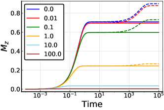
(a)      (b)      (c)

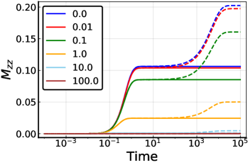
Figure 1: (a), (b) and (c) show the behaviors of three observables $M_{z}$, $M_{c}$, and $M_{zz}$, respectively, as a function of time in the units of $1/J$. To arrive at these plots, the equation (13) has been solved numerically. For each variable, the relative strength of the dipolar interactions and the system-environment coupling was varied by adjusting the ratio $\kappa_{1}^{\star}=\{0,0.01,0.1,1.0,10,100\}.$ The solid lines show the solutions for $\alpha=1$ and the dashed lines show the solutions for $\alpha=0.9999$. In the presence of a completely common environment $\alpha=1$, the system reaches a steady state in agreement with the solutions in Eq. (IV). For $\alpha\neq 1$, the solutions are depicted by dashed lines and the steady states are given by Eq. (IV). We also note the presence of a slow timescale in addition to the fast timescale present for $\alpha=1$ case. The fixed parameter sets are chosen as $\{M_{\circ}=0.9,\kappa_{2}^{\star}=\kappa_{1}^{\star}\}$.

IV.1 Environment-induced entanglement

Entanglement is entirely a quantum mechanical phenomenon of a multipartite system. If a single qubit only interact with it’s local environment, the final steady state is a thermal state, and a thermal state is a non-entangled state. On the other-hand the EIE originating from a CE is a well-known phenomenon since the seminal work of Plenio and others Plenio et al. (1999); An et al. (2007); Benatti et al. (2008); Zhang and Yu (2007); Choi and Lee (2007). We study the growth and the preservation of entanglements in the system through a well-established measure concurrence Wootters (1998); Horodecki et al. (2009). For a bipartite system, the concurrence as a measure was first proposed by Wooters using the eigenvalues of the following Hermitian matrix $\sqrt{\sqrt{\rho_{s}}\tilde{\rho_{s}}\sqrt{\rho_{s}}}$, where $\rho_{s}$ is the given system density matrix and $\tilde{\rho_{s}}=\sigma_{y}\otimes\sigma_{y}\,\rho^{\star}\,\sigma_{y}\otimes\sigma_{y}$. Alternatively, the eigenvalues can be calculated from the non-Hermitian matrix $\rho_{s}\tilde{\rho_{s}}$. If $\lambda_{i}$ are the eigenvalues arranged in the decreasing order, then the concurrence $(C(\rho_{s}))$ is defined as,

$$C(\rho_{s}) = \text{max}\{0,\lambda_{1}-\lambda_{2}-\lambda_{3}-\lambda_{4}\}$$ (17)

If $C(\rho_{s})>0$, then the system has entanglement. For $C(\rho_{s})=0$, we have a separable system. In terms of the observables $\{M_{z},M_{zz},M_{c}\}$, the expression for the steady state entanglement is given by,

$$C(\rho_{s})=\text{max}\{0,2|M_{c}|-\frac{1}{2}\sqrt{(1+4M_{zz})^{2}-4M_{z}^{2}}\}.$$ (18)

The above Eq. (18) corroborates our earlier assertion that there is a possibility of a persistent entanglement if there is a persistent zero quantum coherence, i.e., $M_{c}\neq 0$. But the converse is not true.

Using Eq. (18), we simulate three situations in which the qubit pair may be used as a storage of entanglement. We prepare the system in an initial singlet state $\frac{1}{\sqrt{2}}(|01\rangle-|10\rangle)$ and solve the equations of motion as in Eq. (13) for $\alpha=1$ and for $\alpha=0.9999$. Since the singlet state constitutes a decoherence-free subspace for the entire Liouvillian for $\alpha=1$, hence it remains perfectly preserved as shown by the solid lines in Fig. 2(a). On the other hand, for $\alpha=0.9999$, the singlet state remains preserved for a long time, but eventually decays (the dashed lines in Fig. 2(a)). On the other hand, when we prepare the system in a triplet state $\frac{1}{\sqrt{2}}(|01\rangle+|10\rangle)$, irrespective of the values of $\alpha$, the entanglement decays to zero value at a much shorter time and more so when the dipolar coupling is stronger ($\kappa_{1}^{\star}=100$ case decays faster than $\kappa_{1}^{\star}=0.01$ case). The plots for the triplet case are shown in Fig. 2(b).

Also, as yet another method of generation and storage of entanglement, we prepare the system having a negative dipolar order $M_{zz}=-1/4$. In this condition, we have a strong entanglement build up and perfect preservation for $\alpha=1$ (solid lines in Fig. 2(c)). On the other hand, for $\alpha=0.9999$, the entanglement grows to the same value as that of $\alpha=1$ case and remain preserved for several orders of magnitude of time in terms of 1/J. The entanglement eventually decays to zero value. We note that the timescale of preservation is strongly dependent on the dipolar coupling strength. For $\kappa_{1}^{\star}=1$, the entanglement build-up is small and decays faster than for $\kappa_{1}^{\star}=0.01$. As such, for such storage protocols, the dipolar coupling plays a detrimental role.

To understand the roles of the commonness of the environment $\alpha$ and the effects of the nonsecular dipolar coupling $\kappa_{1}^{\star}$, we plot the maximum value of the concurrence achieved by using the above protocol, for a range of values of $\{\alpha,\kappa_{1}^{\star}\}$. The resulting contour plot is shown in Fig. 3. The contours clearly show that the concurrence is highest for high values of $\alpha$ and low values of $\kappa_{1}^{\star}$.

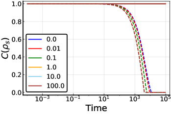
(a)      (b)
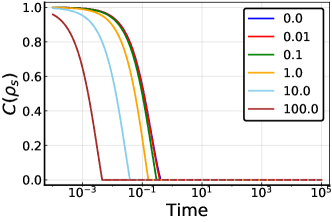
(c)

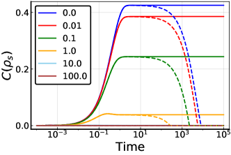
Figure 2: Figure (a) shows the plot of concurrence $C(\rho_{s})$ as a function of time for $\alpha=1$ by solid lines, and $\alpha=0.9999$ by dashed lines, when the system was initially prepared in a singlet state. We observe that the concurrence is perfectly preserved for $\alpha=1$ and decays to zero value for $\alpha<1$. For each $\alpha$ the dipolar coupling (in the scaled unit, $\kappa_{m}^{\star}=\kappa_{m}/J$) has been varied over four orders of magnitude from $1e-2$ to $1e+2$, as shown in the figure legends. Figure (b) shows the plot of concurrence $C(\rho_{s})$ as a function of time for $\alpha=1$ by solid lines, and $\alpha=0.9999$ by dashed lines, when the system was initially prepared in a triplet state. We notice that the triplet state decays almost four orders of magnitude faster than the singlet state. We also observe that stronger dipolar coupling enhances the triplet decay rate. Figure (c) shows the plot of concurrence $C(\rho_{s})$ as a function of time for $\alpha=1$ by solid lines, and $\alpha=0.9999$ by dashed lines, when the system was initially prepared with zero values for all observables. As $M_{c}$ builds up in the system, so does the concurrence according to Eq. (18). However, the concurrence later decays for $\alpha<1$ (shown by dashed lines, as opposed to the solid lines for $\alpha=1$) with a slower timescale. We note that the stronger dipolar coupling enhances the decay rate. The concurrence is preserved for over one order of magnitude of time ($\sim 1/J$) for small dipolar coupling.

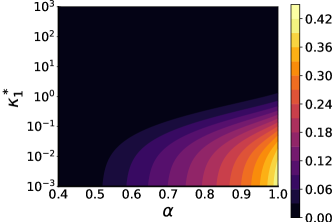
Figure 3: The figure shows the filled contour of the maximum value of $C(\rho_{s})$ a function of $\kappa_{1}^{\star}$ and $\alpha$. The initial state has been chosen to be $M_{z}=M_{c}=0$ and $M_{zz}=-1/4$, which provides the maximum build-up of the entanglements due to a close-to-common environment with $\alpha=0.9999$. To arrive at this plot, equations (13) were solved for a specific choice of $\{\kappa_{1}^{\star},\alpha\}$ and the concurrence has been calculated as a function of time, and the maximum value is selected. We note that the maximum value of the concurrence monotonically increases with increasing $\alpha$, whereas, increasing the dipolar coupling amplitude, the entanglement between the qubits decays. The color range that has been used in the plot is shown in the color bar on the right with the upper and lower bounds of the range. We observe that with the increase of the dipolar coupling, the maximum value of the concurrence decreases.

V Discussions

Fig. 1(b) shows that $M_{c}$ is finite for $\alpha=1$. So, the possibility of persistent EIE only occurs at the critical point $\alpha=1$. For $0<\alpha<1$, the EIE survives at the intermediate time-scale. Fig. 2(c), captures the time-evolution of $C(\rho_{s})$ for $\alpha=0.9999$ and the initial density matrix $\rho_{s}^{ini}=\mathds{1}/4$ $-\left(\sigma_{z}\otimes\sigma_{z}\right)/4$. The EIE, as measured via concurrence, grows and attains maximum value in the intermediate time and finally decays to zero at the steady state. The characteristics of the graph is same as $|M_{c}|$ vs time in the Fig. 1(b). We also show that the value of the $C(\rho_{s})$ decreases for an increase in the dipolar interaction in Fig. 2(c). The second-order dipolar terms dominate over system-environment terms for larger $\kappa_{1}^{\star}$, which results in a faster decay of the entanglement.

In case of the dipolar-interaction, the secular term ($m=0$ in Eq. (2)) does not contribute in the time evolution of the following observables $M_{xx},M_{yy},M_{zz},M_{z}$. We note that the earlier versions of QME are based on the independent rate approximation Claude Cohen-Tannoudji (1998). In such formalism, the secular parts ($m\neq 0$) of the dipolar interactions are taken into account, however secular part does not affect the evolution of the above observables. Since the non-secular contributions had not been included, the previous approaches failed to capture the second-order effect of the following pairs, $m=[\{0,0\},\{1,-1\},\{2,-2\}]$ Heinz-Peter Breuer (2002). In this context, FRQME is clearly a better tool as it incorporates the effect of those terms in the dissipator.

The concepts for the generation and the preservation of EIE is extensively used in quantum storage devices, in the conceptualization of quantum batteries, and environment mediated information transfer processes Tabesh et al. (2020); Farina et al. (2019); Kamin et al. (2020); Gundogan et al. (2012). Our results show that the dissipators from the nonsecular part of dipolar coupling play an obstructive role in this process. It is clear from Fig. 3 that the desirable condition for the maximum sustained concurrence is to reduce $\kappa_{1}^{\star}$ and to increase $\alpha$. One may increase the physical separation between the qubits to reduce $\kappa_{1}^{\star}$. At the same time, it is essential that qubits remain coupled to a common environment with $\alpha\to 1$. Since $\alpha=\exp(-r/\xi)$, we must have $\xi\gg r$, i.e., an environment with a large spatial correlation length much larger than the distance between the qubits. This necessitates a suitably engineered quantum reservoir as a common environment. While there are examples of reservoir engineering Kurizki et al. (2015); Myatt et al. (2000); Rossini et al. (2007), we note that Plenio and others originally reported coupling two physically distant atoms to a lossy cavity Plenio et al. (1999). Such methods will be preferable to an environment created by a tight-binding chain of oscillators since a cavity is much easier to fabricate.

We note that apparently $\kappa_{1}^{\star}$ could be reduced by increasing $J$ i.e., the system-environment relaxation rate, since $\kappa_{1}^{\star}=\kappa_{1}/J$. This would indeed increase the concurrence, as evident in Fig. 3. However, the length of the time over which the entanglement is preserved increases with $1/J$. So, any attempt to increase $J$ will result in a shortening of the entanglement storage time. As such, increasing the qubit separation would be the preferred way to decrease the dipolar effects on the decay of the entanglement.

McCutcheon and others showed that one conceptualization of a spatially-correlated environment was to use a chain of coupled harmonic oscillators. For such an environment, the correlation length of the environment remains a function of the temperature McCutcheon et al. (2009). It is expected that with the decrease of temperature, the correlation length will increase. This facilitates creating efficient storage since the separation of the qubits could be increased. However, we also note that at lower temperatures, the validity of a Markovian quantum master equation may become questionable. Particularly, the crucial assumption of the separation of timescales of the fluctuations and the system dynamics may not hold at very low temperatures since the fluctuations would have a longer correlation time. As such, lowering the temperature may benefit the storage devices, however, the present analysis would probably not be valid at lower temperatures.

VI Conclusion

We demonstrate the detrimental effect of the dipolar interaction on the generation and the preservation of entanglement in a qubit pair that is coupled to a spatially-correlated common environment. Using the formalism of FRQME, we have shown that the second-order contribution of the nonsecular component of the dipolar interaction strongly affects the EIE, which is a major disadvantage for the environment-mediated information storage device. We discuss the efficacy of various engineered environments in mitigating this problem. Our results show that qubits coupled to a spatially correlated lossy cavity would be a preferred solution for entanglement storage.

VII Acknowledgments

The authors thank Arpan Chatterjee and Arnab Chakrabarti for insightful discussions and helpful suggestions. SS acknowledges University Grants Commission for a research fellowship (Student ID: MAY2018- 528071).

Appendix A Fluctuation-regulated quantum master equation

Since the fluctuation-regulated quantum master equation (FRQME) is relatively new, we provide here a brief sketch of its derivation. For more details, the reader may consult the original work of Chakrabarti and others Chakrabarti and Bhattacharyya (2018a).

We consider a driven-dissipative quantum system in the presence of thermal fluctuations. Since the thermal fluctuations are ubiquitous, we explicitly introduce the fluctuations as a separate Hamiltonian. The total Hamiltonian of the system and the environment is written as,

$$\mathcal{H}=\mathcal{H}_{s}^{\circ}+\mathcal{H}_{L}^{\circ}+\mathcal{H}_{\text{\tiny SL}}+\mathcal{H}_{\text{\tiny loc}}+\mathcal{H}_{\text{\tiny L}}(t).$$ (19)

In the above eq-19 the first two terms represent the free Hamiltonian of the system and environment. $\mathcal{H}_{\text{\tiny SL}}$ is the system-environment coupling Hamiltonian. $\mathcal{H}_{\text{\tiny loc}}$ is the local interaction present in the system, e.g. external drive, dipolar interactions, etc. $\mathcal{H}_{\text{\tiny L}}(t)$ is the thermal fluctuation Hamiltonian. The form of $\mathcal{H}_{\text{\tiny L}}(t)$ is given by,

$$\mathcal{H}_{\text{\tiny L}}(t)=\sum_{i}f_{i}(t)|\phi_{i}\rangle\langle\phi_{i}|$$ (20)

where, $\phi$s are the eigenstates of $\mathcal{H}_{L}^{\circ},$ $i$ is the number of energy levels in the bath. Here, $f_{i}$ is modeled as the stationary and delta-correlated, Gaussian stochastic variables with standard deviation $K$. Therefore, $\overline{f_{i}(t)}=0$, $\overline{f_{i}(t_{a})f_{j}(t_{b})}=\frac{1}{\tau_{c}}\delta_{ij}\delta(t_{a}-t_{b})$ and $K^{2}/2=1/\tau_{c}$. Hence, all the coherences in the local environment decays within a time-scale $\tau_{c}$. For a Markovian system, the time-scale of the evolution should be much larger than $\tau_{c}$. In this formalism, we use the coarse-grained prescription provided by Cohen-Tannoudji and others to construct a smooth dynamical equation for the system Claude Cohen-Tannoudji (1998). The coarse-grained time-scale is defined as $\Delta t$, which is assumed to be $\tau_{c}<<\Delta t<<T_{1},T_{2}$. Here $T_{1},T_{2}$ is the system relaxation time-scale. Starting from the von-Neumann Liouville equation of the total density matrix $\rho(t)$ in the interaction frame, the solution at the time-interval $t+\Delta t$ is given by,

$$\rho(t+\Delta t) = \rho(t)-i\int\limits^{t+\Delta t}_{t}[H_{\text{\tiny eff}}(t_{1})+H_{\text{\tiny L}}(t_{1}),\rho(t_{1})]\,dt_{1}$$ (21)

Here, $H_{\text{\tiny eff}}(t)$ is the interaction representation of $\mathcal{H}_{\text{\tiny SL}}+\mathcal{H}_{\text{\tiny loc}}$. The dynamical equation for the system density matrices $\rho_{s}$ can be constructed by taking the partial trace over bath variables on the both side of the eq-21. The commutator including $H_{\text{\tiny L}}(t)$ will vanish by taking the partial trace. In the right-hand side the density matrices can be written as, $\rho(t_{1})=U(t_{1},t)\rho(t)U^{\dagger}(t_{1},t)$, where, $U(t_{1},t)$ is the time evolution operator. The following condition, $\tau_{c}<<1/\omega_{sl},1/\omega_{loc}$ ensures that the time-scale of the fluctuations is much faster than the system-time evolution. Hence, the time-evolution operator must be linear in $H_{\text{\tiny eff}}$ but it contains all possible higher order terms in $H_{\text{\tiny L}}(t)$. The expression of the finite propagator is given by Chakrabarti and Bhattacharyya (2018a),

$$U(t_{1},t) = U_{\text{\tiny L}}(t_{1},t)-i\int^{t_{1}}_{t}dt_{2}H_{\text{\tiny eff}}(t_{2})U_{\text{\tiny L}}(t_{2},t)$$ (22)

Here, $U_{\text{\tiny L}}(t_{1},t)=\mathcal{T}\exp(-i\int\limits_{t}^{t_{1}}H_{\text{\tiny L}}(t_{2})\,dt_{2})$. At the initial time $t$, the system and bath is assumed to be uncorrelated., $\rho(t)=\rho_{L}^{eq}\otimes\rho_{s}(t)$. This is known as Born-approximation Claude Cohen-Tannoudji (1998). By using the form of $U(t_{1},t)$ in eq-21 and taking ensemble average over all $f_{i}$s, the exponential kernel arises in the second order terms of $H_{\text{\tiny eff}}(t)$ $[\overline{U_{L}(t_{1})\rho(t)U^{\dagger}_{L}(t_{2})}=\rho_{L}^{eq}\otimes\rho_{s}(t)e^{-\frac{t_{1}-t_{2}}{\tau_{c}}}]$. The final form of coarse-grained, time-local Markovian master equation given by,

$$\frac{d\rho_{s}}{dt} = -i\,\text{Tr}_{L}\Big{[}H_{\text{\tiny eff}}(t),\rho_{s}(t)\otimes\rho_{L}^{eq}\Big{]}^{sec}$$ (23)

$$-\int\limits^{\infty}_{0}d\tau\,\text{Tr}_{L}\Big{[}H_{\text{\tiny eff}}(t),\Big{[}H_{\text{\tiny eff}}(t-\tau),\rho_{s}(t)\otimes\rho_{L}^{eq}\Big{]}\Big{]}^{sec}e^{-\frac{|\tau|}{\tau_{c}}}$$

The superscript ‘$sec$’ denotes the secular approximation, which requires neglecting the contribution of the higher oscillating term of the FRQME. The above form of FRQME can be reduced to the famous Gorini-Kossakowski-Lindblad-Sudarsan (GKLS) form. Hence trace preservation, and complete positivity also holds for FRQME Chakrabarti and Bhattacharyya (2018a). The main feature of the above eq-23 is the presence of an exponential kernel in the second-order terms, which gives a non-diverging behavior for $H_{\text{\tiny eff}}$ in the dynamics. In the presence of periodic drive, the drive-induced dissipation (DID), drive induced shifts (DIS) originated from the second-order terms Chanda and Bhattacharyya (2020); Chatterjee and Bhattacharyya (2020). Using FRQME, the second-order effect of dipolar interaction in the ‘magic-angle spinning’ (MAS) experiment of NMR spectroscopy has also been studied theoretically by this same authors Saha and Bhattacharyya (2022).

Appendix B Complete set of equations in terms of the observables

The dynamical equation can be written using 15 observables. The equations can be arranged in a block-diagonal from. Equations of each block is presented here. The general form is given by,

$$\dot{A}=\mathbb{L}A+\mathbb{B}$$ (24)

$A$ is the column vector of the observables, $\mathcal{L}$ is the dynamical matrix, $\mathbb{B}$ is the inhomogeneous term.

The first block consist of $A^{T}_{1}=[M_{z}\quad M_{zz}\quad M_{c}]$. the form of $\mathbb{L}$ is given by,

$$\mathbb{L}_{1}=\begin{bmatrix}-2J-\kappa_{1}-4\kappa_{2}&0&4M_{\circ}\alpha J\\ M_{\circ}J&-4J-2\kappa_{1}&2\alpha J+\kappa_{1}\\ -M_{\circ}\alpha J&4\alpha J+2\kappa_{1}&-2J-\kappa_{1}\end{bmatrix}$$ (25)

and $\mathbb{B}^{T}=[2M_{\circ}J\quad 0\quad 0]$. the second block is consist of $A^{T}_{2}=[M_{x}\quad M_{y}\quad M_{xz}\quad M_{yz}]$

$$\scriptstyle\mathbb{L}_{2}=\begin{bmatrix}\scriptstyle-(\frac{5}{2}\kappa_{1}+\kappa_{2}+9\kappa_{0}+J)&\scriptstyle-\frac{\delta\kappa_{1}}{2}-\delta\kappa_{2}+\delta\omega&\scriptstyle-2M_{\circ}J\alpha&\scriptstyle 2M_{\circ}\alpha\delta\omega+6\omega_{d,0}\\ \scriptstyle+\frac{\delta\kappa_{1}}{2}+\delta\kappa_{2}-\delta\omega&\scriptstyle-(\frac{5}{2}\kappa_{1}+\kappa_{2}+9\kappa_{0}+J)&\scriptstyle-(2M_{\circ}\alpha\delta\omega+6\omega_{d,0})&\scriptstyle-2M_{\circ}J\alpha\\ \scriptstyle M_{\circ}J+\frac{M_{\circ}J\alpha}{2}&\scriptstyle\frac{M_{\circ}\alpha\delta\omega}{2}+\frac{3}{2}\omega_{d,0}&\scriptstyle-(\frac{\kappa_{1}}{2}+\kappa_{2}+9\kappa_{0}+3J+2J\alpha)&\scriptstyle-\frac{\delta\kappa_{1}}{2}-\delta\kappa_{2}+\delta\omega\\ \scriptstyle-(\frac{M_{\circ}\alpha\delta\omega}{2}+\frac{3}{2}\omega_{d,0})&\scriptstyle M_{\circ}J+\frac{M_{\circ}J\alpha}{2}&\scriptstyle\frac{\delta\kappa_{1}}{2}+\delta\kappa_{2}-\delta\omega&\scriptstyle-(\frac{\kappa_{1}}{2}+\kappa_{2}+9\kappa_{0}+3J+2J\alpha)\end{bmatrix}$$ (26)

$\mathbb{B}_{2}$ is a null column vector. The third block consists of $A^{T}_{3}=[M_{xy}\quad A_{c}]$. The form of $\mathbb{L}_{3}$ is given by,

$$\mathbb{L}_{3}=\begin{bmatrix}-(\kappa_{1}+2\kappa_{2}+2J)&(\delta\kappa_{1}+2\delta\kappa_{2}-2\delta\omega)\\ -(\delta\kappa_{1}+2\delta\kappa_{2}-2\delta\omega)&-(\kappa_{1}+2\kappa_{2}+2J)\end{bmatrix}$$ (27)

$\mathbb{B}_{3}$ is a null column vector. The fourth block consists of $A^{T}_{4}=[A_{xy}\quad A_{z}]$. The form of $\mathbb{L}_{4}$ is given by,

$$\mathbb{L}_{4}=\begin{bmatrix}-(\kappa_{1}+4\kappa_{0}+2J)&(M_{\circ}\alpha\delta\omega+\omega_{d,0})\\ -4(M_{\circ}\alpha\delta\omega+\omega_{d,0})&-(\kappa_{1}+4\kappa_{0}+2J)\end{bmatrix}$$ (28)

$\mathbb{B}_{4}$ is a null column vector.The fifth block consists of $A^{T}_{5}=[A_{x}\quad A_{y}\quad A_{xz}\quad A_{yz}]$. The form of $\mathbb{L}_{5}$ is given by,

$$\scriptstyle\mathbb{L}_{5}=\begin{bmatrix}\scriptstyle-(\frac{1}{2}\kappa_{1}+\kappa_{2}+\kappa_{0}+J)&\scriptstyle-\frac{\delta\kappa_{1}}{2}-\delta\kappa_{2}+\delta\omega&\scriptstyle 2M_{\circ}J\alpha&\scriptstyle-2M_{\circ}\alpha\delta\omega+2\omega_{d,0}\\ \scriptstyle+\frac{\delta\kappa_{1}}{2}+\delta\kappa_{2}-\delta\omega&\scriptstyle-(\frac{1}{2}\kappa_{1}+\kappa_{2}+\kappa_{0}+J)&\scriptstyle 2M_{\circ}\alpha\delta\omega-2\omega_{d,0}&\scriptstyle 2M_{\circ}J\alpha\\ \scriptstyle M_{\circ}J-\frac{M_{\circ}J\alpha}{2}&\scriptstyle-\frac{M_{\circ}\alpha\delta\omega}{2}+\frac{1}{2}\omega_{d,0}&\scriptstyle-(\frac{\kappa_{1}}{2}+\kappa_{2}+\kappa_{0}+3J-2J\alpha)&\scriptstyle-\frac{\delta\kappa_{1}}{2}-\delta\kappa_{2}+\delta\omega\\ \scriptstyle\frac{M_{\circ}\alpha\delta\omega}{2}-\frac{1}{2}\omega_{d,0}&\scriptstyle M_{\circ}J-\frac{M_{\circ}J\alpha}{2}&\scriptstyle\frac{\delta\kappa_{1}}{2}+\delta\kappa_{2}-\delta\omega&\scriptstyle-(\frac{\kappa_{1}}{2}+\kappa_{2}+\kappa_{0}+3J-2J\alpha)\end{bmatrix}$$ (29)

$\mathbb{B}_{5}$ is also null column vector.

References

- Cabrillo et al. (1999) C. Cabrillo, J. I. Cirac, P. García-Fernández, and P. Zoller, Phys. Rev. A 59, 1025 (1999).
- Plenio et al. (1999) M. B. Plenio, S. F. Huelga, A. Beige, and P. L. Knight, Phys. Rev. A 59, 2468 (1999).
- Beige et al. (2000) A. Beige, S. Bose, D. Braun, S. F. Huelga, P. L. Knight, M. B. Plenio, and V. Vedral, Journal of Modern Optics 47, 2583 (2000).
- Arnesen et al. (2001) M. C. Arnesen, S. Bose, and V. Vedral, Phys. Rev. Lett. 87, 017901 (2001).
- Schneider and Milburn (2002) S. Schneider and G. J. Milburn, Phys. Rev. A 65, 042107 (2002).
- Kim et al. (2002) M. S. Kim, J. Lee, D. Ahn, and P. L. Knight, Phys. Rev. A 65, 040101 (2002).
- Basharov (2002) A. M. Basharov, Journal of Experimental and Theoretical Physics 94, 1070 (2002).
- Jakóbczyk (2003) L. Jakóbczyk, Journal of Physics A: Mathematical and General 36, 1537 (2003).
- Braun (2002) D. Braun, Phys. Rev. Lett. 89, 277901 (2002).
- Benatti et al. (2003) F. Benatti, R. Floreanini, and M. Piani, Phys. Rev. Lett. 91, 070402 (2003).
- Benatti and Floreanini (2004) F. Benatti and R. Floreanini, Phys. Rev. A 70, 012112 (2004).
- Benatti and Floreanini (2006a) F. Benatti and R. Floreanini, Journal of Physics A: Mathematical and General 39, 2689 (2006a).
- Benatti and Floreanini (2006b) F. Benatti and R. Floreanini, International Journal of Quantum Information 04, 395 (2006b).
- Choi and Lee (2007) T. Choi and H.-j. Lee, Phys. Rev. A 76, 012308 (2007).
- Paz and Roncaglia (2008) J. P. Paz and A. J. Roncaglia, Phys. Rev. Lett. 100, 220401 (2008).
- Zell et al. (2009) T. Zell, F. Queisser, and R. Klesse, Phys. Rev. Lett. 102, 160501 (2009).
- McCutcheon et al. (2009) D. P. S. McCutcheon, A. Nazir, S. Bose, and A. J. Fisher, Phys. Rev. A 80, 022337 (2009).
- Jeske and Cole (2013) J. Jeske and J. H. Cole, Phys. Rev. A 87, 052138 (2013).
- Duer (2001) M. J. Duer, Solid State NMR Spectroscopy: Principles and Applications, 1st ed. (Wiley-Blackwell, 2001).
- Saha and Bhattacharyya (2022) S. Saha and R. Bhattacharyya, Journal of Magnetic Resonance Open 10-11, 100046 (2022).
- Bloembergen et al. (1948) N. Bloembergen, E. M. Purcell, and R. V. Pound, Physical Review 73, 679 (1948).
- Chakrabarti and Bhattacharyya (2018a) A. Chakrabarti and R. Bhattacharyya, Phys. Rev. A 97, 063837 (2018a).
- Chakrabarti and Bhattacharyya (2018b) A. Chakrabarti and R. Bhattacharyya, EPL (Europhysics Letters) 121, 57002 (2018b).
- Chanda and Bhattacharyya (2020) N. Chanda and R. Bhattacharyya, Phys. Rev. A 101, 042326 (2020).
- Chatterjee and Bhattacharyya (2020) A. Chatterjee and R. Bhattacharyya, Phys. Rev. A 102, 043111 (2020).
- Smith et al. (1992a) S. A. Smith, W. E. Palke, and J. T. Gerig, Concepts in Magnetic Resonance 4, 107 (1992a).
- Smith et al. (1992b) S. A. Smith, W. E. Palke, and J. T. Gerig, Concepts in Magnetic Resonance 4, 181 (1992b).
- Claude Cohen-Tannoudji (1998) G. G. Claude Cohen-Tannoudji, Jacques Dupont-Roc, Atom-photon interactions: basic processes and applications (Wiley Online Books, 1998).
- An et al. (2007) J.-H. An, S.-J. Wang, and H.-G. Luo, Physica A: Statistical Mechanics and its Applications 382, 753 (2007).
- Benatti et al. (2008) F. Benatti, A. M. Liguori, and A. Nagy, Journal of Mathematical Physics 49, 042103 (2008).
- Zhang and Yu (2007) J. Zhang and H. Yu, Phys. Rev. A 75, 012101 (2007).
- Wootters (1998) W. K. Wootters, Phys. Rev. Lett. 80, 2245 (1998).
- Horodecki et al. (2009) R. Horodecki, P. Horodecki, M. Horodecki, and K. Horodecki, Rev. Mod. Phys. 81, 865 (2009).
- Heinz-Peter Breuer (2002) F. P. Heinz-Peter Breuer, The Theory of Open Quantum Systems (Oxford University Press, 2002).
- Tabesh et al. (2020) F. T. Tabesh, F. H. Kamin, and S. Salimi, Phys. Rev. A 102, 052223 (2020).
- Farina et al. (2019) D. Farina, G. M. Andolina, A. Mari, M. Polini, and V. Giovannetti, Phys. Rev. B 99, 035421 (2019).
- Kamin et al. (2020) F. H. Kamin, F. T. Tabesh, S. Salimi, F. Kheirandish, and A. C. Santos, New Journal of Physics 22, 083007 (2020), publisher: IOP Publishing.
- Gundogan et al. (2012) M. Gundogan, P. M. Ledingham, A. Almasi, M. Cristiani, and H. de Riedmatten, Phys. Rev. Lett. 108, 190504 (2012).
- Kurizki et al. (2015) G. Kurizki, E. Shahmoon, and A. Zwick, Physica Scripta 90, 128002 (2015).
- Myatt et al. (2000) C. J. Myatt, B. E. King, Q. A. Turchette, C. A. Sackett, D. Kielpinski, W. M. Itano, C. Monroe, and D. J. Wineland, Nature 403, 269 (2000).
- Rossini et al. (2007) D. Rossini, T. Calarco, V. Giovannetti, S. Montangero, and R. Fazio, Journal of Physics A: Mathematical and Theoretical 40, 8033 (2007).