Theory-Grounded Measurement of U.S. Social Stereotypes
in English Language Models

Abstract

NLP models trained on text have been shown to reproduce human stereotypes, which can magnify harms to marginalized groups when systems are deployed at scale. We adapt the Agency-Belief-Communion (ABC) stereotype model of Koch et al. (2016) from social psychology as a framework for the systematic study and discovery of stereotypic group-trait associations in language models (LMs). We introduce the sensitivity test (SeT) for measuring stereotypical associations from language models. To evaluate SeT and other measures using the ABC model, we collect group-trait judgments from U.S.-based subjects to compare with English LM stereotypes. Finally, we extend this framework to measure LM stereotyping of intersectional identities.

1 Introduction

Agency	powerless $\leftrightarrow$	powerful		Beliefs				Communion	untrustworthy $\leftrightarrow$	trustworthy
	low status $\leftrightarrow$	high status			religious $\leftrightarrow$	science-oriented			dishonest $\leftrightarrow$	sincere
	dominated $\leftrightarrow$	dominating			conventional $\leftrightarrow$	alternative			cold $\leftrightarrow$	warm
	poor $\leftrightarrow$	wealthy			conservative $\leftrightarrow$	liberal			benevolent $\leftrightarrow$	threatening
	unconfident $\leftrightarrow$	confident			traditional $\leftrightarrow$	modern			repellent $\leftrightarrow$	likable
	unassertive $\leftrightarrow$	competitive							egotistic $\leftrightarrow$	altruistic

Table 1: List of stereotype dimensions and corresponding traits in the ABC model (Koch et al., 2016).

Stereotypes are abstract and over-generalized pictures in people’s minds that capture attributes about groups of people in the complex social world (Lippmann, 1965). They influence people’s thoughts and behaviors, and allow people to make predictions beyond their personal experience or information given (Bruner et al., 1957; Wheeler and Petty, 2001). Stereotypes are also entwined with the production of prejudice, discrimination, and in-group favoritism (Stangor, 2014; Jackson, 2011). A long line of research in social psychology has established models of generic dimensions that estimate people’s stereotypes of social groups (Koch et al., 2016; Fiske et al., 2002, i.a.). We build on the Agency Beliefs Communion (ABC) model, which measures stereotypes toward a social group with respect to 16 traits in three dimensions: Agency/Socioeconomic Success, Conservative–Progressive Beliefs, and Communion (§ 2); an analysis of the group “man” across 32 traits (16 opposing dyads) is shown in Figure 1.

Pre-trained language models (LMs) encode correlations between social groups and traits, like associating the group “Muslim” with the trait threatening, or “man” with confident (e.g., Bender et al., 2021; Nozza et al., 2021; Hovy and Yang, 2021). We conduct a systematic study of social stereotypes in contextualized English masked LMs, grounded in group-trait associations from the ABC model. To capture the group-trait associations in the LM, we first assess two previously proposed word association tests and also propose a new measurement: the sensitivity test (SeT) (§ 3).

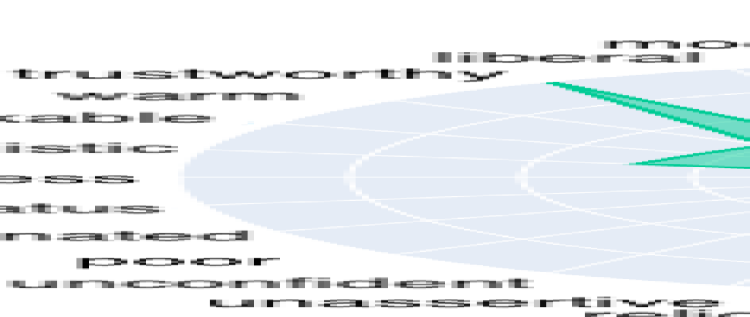
Figure 1: Crowdsourced analysis of the social group “man” under the ABC model (Koch et al., 2016). Colors: purple=agency, red=belief, green=communion.

To evaluate the degree to which two LMs—BERT (Devlin et al., 2019) and RoBERTa (Liu et al., 2019)—align with human stereotype judgments, we design a human study for collecting group-trait judgments (§ 4). We show that our measure, SeT, best aligns with human judgements on group-trait associations and find that, in general, the association from language models have moderate alignment with human judgements.

Finally, with the best-aligned association measurement, we extend the ABC approach to study LM stereotypes on intersectional groups (§ 5.2). Due largely to the difficulty of extending current approaches for measuring stereotypes in LMs to large numbers of groups, most current approaches only study isolated groups, despite the fact that people’s social identities are multifaceted (Ghavami and Peplau, 2013). Because our approach is generalizable to unstudied groups, we take a step towards exploring stereotypes of intersectional identities, finding some correspondence between model behavior and the literature on intersectional stereotypes.

2 Background and Related Work

People’s impressions of the world and the actions they take are guided by their stereotypes. To systematize this observation, the field of social psychology has proposed models of stereotypes, including traits that can coordinate social behaviors to serve as fundamental dimensions of stereotyping. Some models are designed to focus on social evaluation towards individual persons (Abele and Wojciszke, 2014), ingroup members (Ellemers, 2017; Yzerbyt, 2018), or a small set of outgroups (Fiske et al., 2002); the Agency Beliefs Communion (ABC) model—whose traits are designed to distinguish groups—is suited for a larger set of U.S. social groups (Abele et al., 2020). The ABC model takes a data-driven strategy to select a set of traits by eliminating those that are less effective in capturing stereotypes. The list contains $16$ pairs, where each pair represents two polarities (see Table 1), categorized into three dimensions: agency/socioeconomic success, conservative-progressive beliefs, and communion/warmth.

Ours is far from the first work to assess stereotypes in language models, and has both advantages and disadvantages compared to previous approaches (see Table 2). Past work has generally taken one of two approaches. The first approach tests systems with hand-constructed templates like “The [group] is $\square$”, where [group] ranges over social groups (e.g., “woman” or “Hispanic”), and $\square$ represents a “masked word” and ranges over occupations (“a professor” or “a nurse”) (e.g., Bolukbasi et al., 2016; May et al., 2019) or associations drawn from implicit association tests (IAT) (e.g., pleasant/unpleasant words or career/family-related words) (e.g., Caliskan et al., 2017; Guo and Caliskan, 2021). In Table 2 we refer to these as “unnatural” prompts. The second approach collects more natural sentences containing stereotypes, either by web crawling with crowdworkers annotations for social bias (Sap et al., 2019) or by having crowdworkers directly write stereotyping sentences (Nangia et al., 2020; Nadeem et al., 2020).

Measurement	Generalizes	Grounded	Exhaustive	Natural	Specificity
Debiasing (Bolukbasi et al.)	✓				✓
CrowS-Pairs (Nangia et al.)			✓	✓	✓
Stereoset (Nadeem et al.)			✓	✓	✓
S. Bias Frames (Sap et al.)			✓	✓​​✓	✓
CEAT (Guo and Caliskan)	✓	✓		✓​​✓
This Work	✓	✓	✓​​✓

Table 2: Comparison with previous work: Generalizes denotes approaches that naturally extend to previously unconsidered groups; Grounded approaches are those that are grounded in social science theory; Exhaustiveness refers to how well the traits cover the space of possible stereotypes; Naturalness is the degree to which the text input to the LM is natural (we consider naturally occurring web scraped data as “very natural” and crowdsourced sentences as “somewhat natural.”). Specificity indicates whether the stereotype is specific or abstract.

In our work, we take the first approach with traits from the ABC model, using prompts. The advantage of this approach is that the templates and the traits are completely controlled and are easy to extend to other social groups. The second approach is harder to control, which also leads to significant annotation challenges (Blodgett et al., 2021). Using natural sentences limits generalizability, as it requires a unique collection of prompts (and embedded traits) for each social group; in contrast, the prompt-based approach easily generalizes to any plausible group, especially when based on a theoretically grounded framework like ABC or IAT.

An advantage of our work is that the ABC traits are more exhaustive in stereotype coverage with verification from social psychological experiments. The ABC model covers three dimensions with 16 traits, which are consensual, spontaneous, and have been tested using expansive range of social groups (Koch et al., 2021). They used a carefully designed data-driven approach to gather people’s fundamental dimensions of social perceptions with as little sampling bias as possible. Thus the resulted 16 traits cover most stereotypes.

Nevertheless, the main trade-off of our approach is that the testing data are not as natural and specific as other approaches. Although we carefully pick and adjust the templates and the form of the social group terms so that the testing sentences are grammatically correct, they are likely not representative of sentences seen in the real world or in the training data of the language models. Further, while our approach has the benefit of near-exhaustive coverage of potential stereotypes, this comes at a cost: the traits we consider are much more high level (e.g., “repellent”) than more fine-grained stereotypes collected by other means (e.g., the angry Black woman stereotype Collins (2002))—this approach therefore trades coverage for specificity.

3 Measuring Stereotypes in LMs

Domain	Groups
Gender/ sexuality	man, woman, non-binary, trans, cis, gay, lesbian
Race/ ethnicity	Black, White, Hispanic, Asian, Native American
Religion	Jewish, Muslim, Christian, Buddhist, Mormon, Catholic, Amish, Protestant, Atheist, Hindu
Socio-economic	wealthy, working class, immigrant, veteran, unemployed, refugee, doctor, mechanic
Age	teenager, elderly
Disability status	blind, autistic, neurodivergent, Deaf, person with a disability
Politics	Democrat, Republican
Nationality	Mexican, Chinese, Russian, Indian, Irish, Cuban, Italian, Japanese, German, French, British, Jamaican, American, Filipino

Table 3: Social groups domains and corresponding social groups used for the model experiments and human experiments. Single groups for human experiments are highlighted with italic font style.

Our goal is to measure stereotypes in (masked) LMs, and compare them to stereotypes elicited from people. In § 4 we describe our approach for eliciting human judgments of group-trait affinities; here we describe how we measure these in LMs. Previous work has proposed various ways to measure word associations in LMs, including increased log probability score (ILPS) and contextualized embedding association test (CEAT), both of which we summarize below. Finally, we present a new measurement which we call the Sensitivity Test (SeT), which adapts concepts from active learning to the task of measuring a LM’s associations.

3.1 Measurements of Word Associations

Increased Log Probability Score (ILPS)

quantifies word associations in language models through masked word probabilities. It calculates the association score with a pre-defined template, “[Group] are $\square$.” (Kurita et al., 2019), where $\square$ is a masked token. For example, given a group “Asian” and a trait smart, $P(\text{``}Asian\text{''},\texttt{smart})$ measures the probability of smart given “Asians” by filling in the template. Since this probability is affected by the prior probability of smart, ILPS normalizes this probability by the “prior” probability of the trait given a masked group, as below:

$$\textrm{ILPS}(\texttt{g},\texttt{t}) =\log\frac{P({\square}=\texttt{t}\textrm{ | {g} are {$\square$}.})}{P({\square}_{2}=\texttt{t}\textrm{ | {$\square$} ${}_{1}$ are {$\square$} ${}_{2}$.})}$$

Intuitively, ILPS measures how much each group raises the likelihood of a trait filling in the template. One can easily show that this equivalent to the weight of evidence of the trait in favor of the hypothesis that the group is the target: $s(\texttt{g},\texttt{t})=\textrm{woe}(\texttt{g}:\texttt{t}~{}|~{}\textrm{template})$ (Wod, 1985).

Singular	Plural
The/That/A [group] is $\square$.	Most/Many/All [group] are $\square$.  / [Group] are $\square$.
Declarative	Interrogative
[Group] are $\square$.	Why are [group] $\square$?
Non-adverbial	Adverbial
[Group] are $\square$.	[Group] are very/so/mostly $\square$.
Fact	Belief
[Group] are $\square$.	I/We/Everyone/People believe/expect/think/know(s) that [group] are $\square$.
Fact	Social Expectation
[Group] are $\square$.	[Group] are supposed to be/should be/are seen as/ought to be/are expected to be $\square$.
Group-first	Trait-first
[Group] are $\square$.	The $\square$ people are [group].
Non-comparative	Comparative
[Group] are $\square$.	[Group] are more likely to be $\square$ than others.

Table 4: Template Variations.

Contextualized Embedding Association Test (CEAT)

estimates word associations with word embedding distances (Guo and Caliskan, 2021). Intuitively, CEAT measures whether some groups are closer to certain traits in a latent vector space. CEAT is a function of $A,B,X,Y$. Given two sets of target words defining groups $X,Y$ (e.g. $X_{\textrm{male}}=\{$“man”, “father”, …$\}$, $Y_{\textrm{female}}=\{$“woman”, “mother”, …$\}$) and two sets of polar traits $A,B$ (e.g. $A_{\textrm{pleasant}}=\{$ love, peace, …$\}$, $B_{\textrm{pleasant}}=\{$ evil, nasty, … $\}$), CEAT computes the effect sizes of the difference between $X$ and $Y$ being closer to $A$ than $B$ and corresponding p-values. Since contextualized word representations are affected by the contexts around the word, for each word in the four word sets, CEAT randomly samples $1000$ sentences from Reddit, in which the word appears, and uses these to approximate the true effect size as below:

$$\textrm{CEAT}=\frac{\scriptstyle\underset{\scriptscriptstyle\texttt{g}\sim X}{\hat{\mathbb{E}}}s(\texttt{g},A,B)-\underset{\scriptscriptstyle\texttt{g}\sim Y}{\hat{\mathbb{E}}}s(\texttt{g},A,B)}{\scriptstyle\underset{\scriptscriptstyle\texttt{g}\sim X\cup Y}{\hat{\mathbb{S}}}s(\texttt{g},A,B)}\\ s(\texttt{g},A,B)$$

,where

$$s(\texttt{g},A,B)=\underset{\scriptscriptstyle\texttt{t}\sim A}{\hat{\mathbb{E}}}\textrm{cos}(\vec{\texttt{g}},\vec{\texttt{t}})-\underset{\scriptscriptstyle\texttt{t}\sim B}{\hat{\mathbb{E}}}\textrm{cos}(\vec{\texttt{g}},\vec{\texttt{t}})$$

$\hat{\mathbb{E}}$ (resp. $\hat{\mathbb{S}}$) is the empirical expectation (resp. standard deviation), and $\vec{\texttt{x}}$ denotes the embedding of x.

In our setting, since we care about social bias among multiple groups rather than the difference between two groups, we modify the CEAT to calculate the effect size of the distance difference between g with $A$ and $B$ for each group as below:

$$\textrm{CEAT}(\texttt{g},A,B)=\frac{\underset{\scriptscriptstyle\texttt{t}\sim A}{\hat{\mathbb{E}}}\textrm{cos}(\vec{\texttt{g}},\vec{\texttt{t}})-\underset{\scriptscriptstyle\texttt{t}\sim B}{\hat{\mathbb{E}}}\textrm{cos}(\vec{\texttt{g}},\vec{\texttt{t}})}{\underset{\scriptscriptstyle\texttt{t}\sim A\cup B}{\hat{\mathbb{S}}}\textrm{cos}(\vec{\texttt{g}},\vec{\texttt{t}})}$$

Sensitivity Test (SeT)

is a new approach we propose to measure word association for social bias in language models, inspired by ideas from active learning Beygelzimer et al. (2008). The intuition of SeT is that even though a model assigns the same probability to two different words, the robustness of those two probabilities may be different. For example, both $p(\texttt{competent}|\textit{``Blind people are {$\square$}.''})$ and $p(\texttt{kind}|\textit{``Men are {$\square$}''})$ might be low. However, the language model may well not have seen many examples with blind people, as opposed to the presumably very large number of examples of men. In this case, a small number of examples may be sufficient to alter the model’s predictions about blind people, while a larger number would be required for men. SeT captures the model’s confidence in a prediction by measuring how much the model weights would have to change in order to change that prediction. Specifically, SeT computes the minimal change to the last-layer of the language model so that a given trait becomes the highest probability trait (over the full vocabulary).

For example, consider the template “The [group] is $\square$.” with the group “woman” and the trait incompetent. Let $\boldsymbol{\ell}$ be the logits at $\square$ when the input is “The woman is $\square$.”, and let t be the index of incompetent in $\boldsymbol{\ell}$ (so that $\ell_{\texttt{t}}=p(\texttt{incompetent}~{}|~{}\textrm{context})$). Let $\mathbf{h}$ be the last hidden layer before the logits, and let A be the matrix of the last linear layer so that $\boldsymbol{\ell}=\textbf{A}\mathbf{h}$. SeT computes the minimal distance between A and some other matrix $\textbf{A}^{\prime}$ so that t is the top word among the new logits $\boldsymbol{\ell}^{\prime}=\textbf{A}^{\prime}\mathbf{h}$. Formally:

$$\textrm{SeT}(\texttt{g},\texttt{t}) =\log\frac{\Delta(\textbf{A},\mathbf{h}_{\texttt{g}},\texttt{t})}{\Delta(\textbf{A},\mathbf{h}_{\square},\texttt{t})}$$

where $$\mathbf{h}_{\texttt{g}}\textrm{ is the penultimate layer on input {g}}$$

A is the matrix before the logits

$$\Delta(\textbf{A},\mathbf{h},\texttt{t}) =\min_{\textbf{A}^{\prime}}\|\textbf{A}^{\prime}-\textbf{A}\|_{2}^{2}$$

$$~{}~{}~{}\text{ s.t. }(\textbf{A}^{\prime}\mathbf{h})_{\texttt{t}}\geq(\textbf{A}^{\prime}\mathbf{h})_{\texttt{t}^{\prime}}+\gamma\text{, }\forall\texttt{t}^{\prime}\neq\texttt{t}$$

for a fixed margin $\gamma>0$, which we set to $1$. SeT returns the negative distance as measure of the association between the corresponding group and trait, normalized by a prior akin to ILPS. This optimization problem does not (to our knowledge) admit a closed form solution; we solve it iteratively using the column squishing algorithm (Bittorf et al., 2012; Daumé and Kumar, 2017).

3.2 Implementation details

We test the above measurements on both BERT and RoBERTa pretrained large models from an open-source HuggingFace library.

Social groups.

Table 3 lists all the individual social groups we cover in this work. We manually construct the list by combining and picking groups from the list of social groups from Sotnikova et al. (2021) and Koch et al. (2016) and also adding social groups we think are stereotyped in U.S. culture.

Traits.

We use the 32 adjectives of the 16 traits from the ABC model (Table 1). For each traits, we calculate the score of its left-side adjective from its right-side adjective: $S_{\texttt{powerless-powerful}}(\texttt{g})=S(\texttt{g},\texttt{powerful})-S(\texttt{g},\texttt{powerless})$, where $S$ is one of the scores from § 3.1.

Templates.

ILPS and SeT both require templates in calculating scores. We thus carefully construct a list of templates (Table 4) that covers multiple grammatical and semantic variations, inspired by work investigating harmful search automatic suggestions (Hazen et al., 2020). We find that different model structure requires different templates in order to bring up stereotypes that correlate with human data. See § 5 for evidence.

Subwords.

Due to the nature of BERT and RoBERTa’s tokenizers, some of the adjectives are divided into multiple subwords. This is problematic because all the measurements compute their scores at token level. Neither ILPS nor CEAT deals with subwords directly: in their released implementations, they either take the first or the last sub-token of the word. To remedy this, we adjust the ILPS measurement (denoted as ILPS^⋆) to properly compute the probability of traits in context using the chain rule across subwords. For SeT, we calculate the sensitivity score for each subword individually and take the maximum SeT score as the SeT score for the word, which effectively computes a lower-bound on how much the model parameters would need to change. We did not modify CEAT’s measurement as it is not clear what is the best way to compute comparable word embeddings for words that consist of multiple subwords.

4 Human Study

In the previous section, we describe how we compute associations between groups and traits in language models. In this section, we assess stereotypes of social groups through groups-trait association, like in Figure 1. We adopt this approach because it is widely used to evaluate group stereotypes in social psychology field (Fiske et al., 2002; Koch et al., 2016). It also aligns with Lippmann (1965)’s theory of stereotypes that they are abstract pictures in people’s head. We broadly follow procedures from previous social psychology papers to collect human evaluation on social groups.

Survey Design.

We recruit participants from Prolific. Each participant is paid $\$2.00$ to rate $5$ social groups on $16$ pairs of traits and on average participants spend about $10$ minutes on the survey. This results in a pay of $\$12.00$ per hour. Maryland’s current minimum wage is $\$12.20$ . First, participants read the consent form, and if they agree to participate in the study, they see the survey’s instructions. For each social group, participants read "As viewed by American society, (while my own opinions may differ), how [e.g., powerless, dominant, poor] versus [e.g., powerful, dominated, wealthy] are <group>?" They then rate each trait with a $0$-$100$ slider scale where two sides are the two dimensions of the trait (e.g. powerless and powerful). Each annotated group is shown on a separate page, and participants cannot go back to previous pages. To avoid social-desirability bias, we explicitly write in the instruction that “we are not interested in your personal beliefs, but rather how you think people in America view these groups.”

Participant Demographics.

At the end of the survey we collect participants’ demographic information, including gender, race, age, education level, type of living area, etc. Our participants represent $26$ states, with $63.3\%$ from California, New York, Texas, or Florida; the gender breakdown is $48.2\%$ male, $49.6\%$ female, and $2.2\%$ genderqueer, agender, or questioning; and skew young, with over $96\%$ at most $40$ years old; and with racial demographics that approximately match the U.S. census. For more details on demographics, see Appendix E.

Quality Assurance.

Ensuring annotation quality in a highly subjective task is a challenge, and common approaches in NLP like having questions where we “know” the answer as tests, measuring interannotator agreement, and calibrating reviewers against each other (Paun et al., 2018) do not make sense here. Yet, it is still important to ensure the annotation quality. After much iteration, we include three test questions, and warn the participants at the beginning that there are test questions.

1. After the first group, participants must name the group they just scored.

2. After the second, participants must list one trait they just marked high and one marked low.

3. The fifth (final) group is a repetition of one of the four groups they previously scored.

We discard annotations with incorrect answers to either of the first two questions. For the third test, we compute intra-annotator (self) agreement and discard annotations with accuracy-to-self lower than $80\%$. For each group we collect $20$ annotations that pass our quality threshold. In total, we collected annotations from $247$ participants, with $133$ passing the quality tests (suggesting that having such tests is important). The $114$ annotations that did not pass tests were excluded from our dataset, but all $247$ participants were paid.

Social groups and traits.

The social groups we used for the human study are highlighted in Table 3. This table contains only single groups used for the model § 3 and human experiments. We collect annotations for $25$ social groups within $5$ domains, across all $16$ pairs of traits.

5 Results

	RoBERTa			BERT
Measure	$\tau$	Template(s)		$\tau$	Template(s)
ILPS	0.280	That [group] is [trait].		0.215	All [group] are [trait]. [Group] should be [trait].
ILPS⋆	0.258	All [group] are [trait]. That [group] is [trait].		0.123	We expect that [group] are [trait]. [Group] should be [trait].
SeT	0.253	That [group] is [trait].		0.214	All [group] are [trait]. [Group] should be [trait].

Table 5: Best two templates for each measurement-model pair and corresponding correlations. Some have only one template because there is no combination of two templates that give higher correlation score than this one template.

In this section we present results on correlations between human and model stereotypes for individual groups, comparing across different measurements, including our proposed measurement, SeT (§ 5.1). Next, we analyze how model scores change for intersectional social groups. We consider several possible factors that may influence the score changes such as identity order, some domain domination, and consider emergent traits (§ 5.2).

	CEAT		ILPS		ILPS⋆		SeT
	RoBERTa	BERT	RoBERTa	BERT	RoBERTa	BERT	RoBERTa	BERT
Kendall’s $\tau$	0.019	0.111$\dagger$	0.169$\dagger$	0.094$\dagger$	0.175$\dagger$	0.015	0.199$\dagger$	0.116
Precision at 3	0.500	0.587$\dagger$	0.620$\dagger$	0.533$\dagger$	0.653$\dagger$	0.560	0.653$\dagger$	0.613

Table 6: Overall alignment scores with human annotations. The highest scores are bold for each row. For correlation scores, we mark scores where the p-value is $<0.05$ with $\dagger$.

5.1 Correlation on Individual Groups

Before we answer the question of how language model stereotype scores align with human stereotypes across the measurements introduced in § 3, we first run a pilot experiment to select the best template(s) for each measurement-model pair from the set of templates in Table 4 (except for CEAT, which does not require templates). We randomly picked four social groups (Asian, Black, Hispanic, immigrant) and five annotations from each group for the pilot. Since our goal is to inspect the alignment between human and model stereotypes, we take the averaged score of the five annotations as “ground truth” and select templates that give the correlation score according to Kendall $\tau$. We limit the selection to at most two templates to avoid overfitting on the pilot data, selected to maximize correlation for each measurement-model pair.

The selected templates and corresponding correlation scores are shown in appendix (Table 5); the score range for weak correlation is $0.10$ - $0.19$, moderate $0.20$ - $0.29$, and strong $0.30$ and above Botsch (2011). For a fixed LM, the best templates tend to be similar across all measures: RoBERTa tends to achieve highest correlation with templates like “That [group] is [trait].” while for BERT the preferred templates tend to be “All [group] are [trait].” or “[Group] should be [trait].”

Given the best templates for each measurement-model pair, we measure to what degree language model stereotypes are aligned with human stereotypes with all annotations on 25 social groups. To quantify alignment, we both calculate the Kendall rank correlation coefficient (Kendall’s $\tau$) and the Precision at 3 (P@3). The former indicates the correlation between model and human scores on group-trait associations in terms of the number of swaps required to get the same order. The latter indicates the percentage of the model’s top stereotypes which accord with human’s judgements. For P@3, we also calculate at both the group level and overall with all groups. For each group, we compute its P@3 score by taking the average of the P@3 scores with the top 3 traits (top at one polarity) and the score with the bottom 3 (top at the other polarity) because each trait has two polar adjectives and the group-trait score is calculated with the difference of the two polarities. To calculate the P@3 scores, we binarize the human group-trait scores at a threshold of $50$. The overall P@3 score is the average of the groups’ individual P@3 scores.

The overall scores are in Table 6. We see that in general that RoBERTa contains group-trait associations that are more similar to human judgements than does BERT. Additionally, we see that both ILPS^⋆ and SeT have higher P@3 scores than CEAT and ILPS. The RoBERTa model with the SeT measurement approach yields outputs are the most aligned with human’s judgements, with RoBERTa/ILPS^⋆ a close second. From its scores, we see that model’s group-trait associations have moderate correlation with human’s judgements. Moreover, in general, two out of the three top ranked group-trait associations from the model agree with human data. See Table A19 for the overall scores of test groups only, where the four pilot groups are excluded, and Appendix B for group level alignment scores.

5.2 Intersectional Groups in LMs

Background.

Intersectionality is a core concept in Black feminism, introduced in the Combahee River Collective Statement in 1977 (1977; 1983), considering the ways in which feminist theory and antiracism need to combine: “Because the intersectional experience is greater than the sum of racism and sexism, any analysis that does not take intersectionality into account cannot sufficiently address the particular manner in which Black women are subordinated.” The concept was applied in law by Crenshaw (1989) to analyze the ways in which U.S. antidiscrimination law fails Black women.

The concept of intersectionality has broadened and, while its boundaries remain contested (e.g., Browne and Misra, 2003), there are a number of core principles that are central (Steinbugler et al., 2006; Zinn and Dill, 1996): (1) social categories and hierarchies are historically contingent, (2) the experience at an intersection is more than the sum of its parts Collins (2002); King (1988), (3) intersections create both oppression and opportunity Bonilla-Silva (1997), (4) individuals may experience both advantage and disadvantage as a result of intersectionality, and (5) these hierarchies impact social structure and social interaction.

Goals and Research Questions.

We aim to understand whether we can measure evidence of intersectional behavior in language models with respect to stereotyping. In particular, we are interested in questions surrounding how language models stereotype people who simultaneously belong to multiple social groups. We will only use the term “intersectionality” when specifically considering cases where (per (3) above) the resulting experience (in this case, stereotyping) is more than the sum of its parts. For example, common U.S. stereotypes for Black women are as “welfare queens” (which may show up as low agency in our traits), while common stereotypes for Black men is as “criminal” (which may show up as low communion) (hooks, 1992; Collins, 2002). To limit our scope, we will only consider pairs of social groups (e.g., cis men), and will refer to the the groups that make up a pair as the component identities (e.g., cis, or men). We aim to answer the following research questions:

1. When presented with a paired identity, is the language model sensitive to the order in which the component identities appear?

2. When paired, do certain social categories dominate others in a language model’s predictions?

3. Can the language model detect stereotypes that belong to an intersectional group (but not to either of the components that make up the pair)?

To answer these questions, we use the SeT measurement with the RoBERTa model (the best performing pair on the single-group experiments) to compute group-trait associations on our paired groups, which are combinations of all the single groups in Table 3. We manually omit the groups that do not logically exist (e.g. “cis non-binary person”, “teenage elderly person”) or are grammatically awkward (e.g. “doctor elderly person”, “immigrant blind person”). Note we include both orders of the single groups in the paired groups when possible (e.g. “Catholic teenager” and “teenage Catholic person”). We then conduct the analysis by computing the correlation between groups’ list of trait scores with Kendall’s $\tau$.

Q1: Identity Order.

Given an paired group with two identities, the language model may not be able to capture both of the identities and may predict stereotypes based only on one of the components. In fact, the average correlation score between a paired group and the most correlated of its components is $0.56$, which is moderately high. We thus calculate the correlation of trait scores between the paired group and both its first and second component identities (when both orders are possible). In addition, we calculate the correlation of paired groups with reversed identity order (e.g. “Asian teenager” and “teenage Asian person”). The average correlation score between a paired group and its first component is $0.43$; the correlation score to its second component is $0.46$, which are quite close. Further, the average correlation score of intersectional groups with reversed identity is $0.69$, which is moderately high. Taken together, these results indicate that (a) many paired groups have similar group-trait association scores with one of their component identities alone; (b) the order does not matter significantly, but the language model tends to focus slightly more on the second component. The implication of this is that we can expect that the language model may be able to capture intersectional stereotypes.

Q2: Dominant Domains.

Stryker (1980) suggests that people tend to identify themselves with their race/ethnicity identity before other identities, though this is contested and, in some cases, thought to be antithetical to the idea of intersectionality (e.g., Collins, 2002). Prompted by this debate, we ask if there is a hierarchy of the domains that language model picks up on for paired groups. To answer this question, for each identity domain pair, we compute the average correlation score between the paired groups with each of its two component identities, and take the difference of the averaged correlation scores of the two domains. For each domain, we count the domains it dominates (i.e. has score difference $\geq 0.1$) and is dominated by.

These results show that age and political stance are dominant domains, which is expected as identities within these two domains have strong characteristics that may overwhelm domains they are paired with. On the other end, race and nationality are, generally, dominated domains. It is surprising that the race domain is majorly dominated, contrasting documented literature in human behavior. The full results are shown in Appendix Table A8 as well as detailed scores Table A9.

Q3: Emergent Intersectional Stereotypes.

Finally, we look into emergent stereotypes of paired groups, with the goal of finding intersectional behavior in the language model. To detect intersectional stereotypes, we need to operationalize the notion of the whole being greater than its parts. For a fixed paired group $\texttt{g}=(\texttt{g}_{1},\texttt{g}_{2})$ (e.g., “trans Democrats”), and a given trait t (e.g., warm), we compute $S(\texttt{g},\texttt{t})-\max\{S(\texttt{g}_{1},\texttt{t}),S(\texttt{g}_{2},\texttt{t})\}$, where $S$ is the score from the language model, capturing whether this trait is more associated with the paired group than the maximum of its association with the component identities. (We consider also the reverse, where we look for scores much less than the min.) We might hope to find some well attested intersectional identities from the literature, such as “Black women” have an attitude (low communion) and “White men” are privileged (high agency)  (Ghavami and Peplau, 2013).

The top $50$ emergent group-trait associations according to our measure are listed in Table A10. We also see some good examples are: the language model scores “Hispanic unemployed people” as more egotistic than people of the component identities, “Democrat teenagers” as more altruistic, “male doctors” as more benevolent, etc. However, there are also some unexpected patterns; for instance, almost all nationality identities combined with “mechanic” are trustworthy and likeable, and almost all nationality identities combined with “autistic” are egotistic. Looking into the scores themselves, we find that both “mechanic” and “autistic” have low scores on the corresponding traits, and combining them with nationalities raises to about average levels.

Aside from analyzing face validity—which is mixed—we compare the results of our model to the traits that Ghavami and Peplau (2013) found when conducting human studies of race/gender pairs. To do this, we categorize the traits from Ghavami and Peplau (2013) to the ABC dimensions and compare with our full list of emergent group-trait associations. Taking their group-trait matches as ground truth, our detection of traits for these race/gender intersectional groups achieves a precision $0.83$ and recall $0.65$—better than random guessing (precision $0.72$, recall $0.50$) but far from perfect.

6 Limitations and Ethical Considerations

There are several limitations to our work, which should be taken into account in the interpretation of our results.

First, our results are likely affected by reporting bias and by a defaulting effect where, when people annotate traits for “men”, they may actually have in their head “cis straight white men”, because the defaults go unremarked. This goes both for the human scores (how does a participant conceptualize “men”?) and language model scores (what do sentences containing the word “man” assume given that most language a langauge model has been trained on likely exhibits defaulting?).

Second, our work only focus on assessing stereotypes within language models and not in any deployed system. Though stereotypes from language models may impact the outputs of downstream systems which are built upon these language models, it is not clear how exactly the stereotypes transfer (Cao et al., 2022). Additionally, our work is limited to English and U.S. social stereotypes.

Third, although we followed and built on best practices from social psychology in developing the human study, it nevertheless has some shortcomings. In particular, even after many iterations on wording, it was difficult to phrase the survey questions to encourage people to reporting their true impressions. There is tension between asking a participant what they think—which risks a counfounding potential social desirability bias (Latkin et al., 2017) (people’s tendency to respond in socially acceptable ways)—and asking what they think others think—which led to comments from a few participants that they felt unqualified to speak for others. Asking these questions of participants and collecting the data also raises the possibility of this work inadvertantly reinforcing stereotypes.

Finally, aggregating human judgements into a single number by averaging (or any other statistic) to compare to model predictions risks collapsing a significant amount of information down to a single number. This number cannot distinguish between a weakly held but common stereotype and a strongly held but rare one. Nor can it distinguish between traits where half of annotators say 0 and the other half say 100, from traits where all annotators say 50. These average judgments should be interpreted as not what any single person would say, but an average over people. This limitation is exacerbated by the defaulting effect, where some people may imagine a different prototype for a given group, and other people may imagine another.

7 Conclusion

In this paper, we measured language model (LM) stereotypes by adopting the ABC stereotype model from social psychology. Comparing to previous work on detecting LM stereotypes, our approach is easy to extend to previously unconsidered groups, grounded in traits proven effective by social psychology, and exhaustively covering the space of possible stereotypes, at the cost of being more abstract than in other NLP work. This yields a different set of trade-offs than previous approaches to measuring stereotypes in LMs.

With the ABC model and data regarding human stereotypes from our human study, we assessed LM stereotypes using three different association measurements, including SeT, a metric we proposed. We showed that LM group-trait stereotypes in general have moderate correlation with human judgements, and that SeT provides correlations that better align with human’s. Based on these results, we extended our analysis to intersectional groups. We found that the LM may be able to capture intersectional stereotypes but is not particularly good on identifying emergent intersectional stereotypes. Our results also show that that, in general, age and political stance are dominant domains in language models, whereas race and nationality are dominated domains. We hope that our work provides insights for future works on measuring and mitigating stereotypes in natural language processing systems, and that the grounding in theories from social psychology has benefits beyond just studying stereotypes.

Appendix A Traits

The full list of traits and respective adjectives is in the Table A7

Trait	Adjectives
Agency scale
Powerful	forceful, formidable, capable
Powerless	weak, helpless, incapable
High status	privileged, elite, advantaged
Low status	unskilled, lowly, inferior
Dominant	commanding, authoritative
Dominated	subservient, submissive, deferential
Wealthy	affluent, rich, prosperous
Poor	impoverished, destitute, needy
Confident	self-assured, assured, self-possessed
Unconfident	bashful, meek, timid
Competitive	ambitious, driven, zealous
Unassertive	submissive, diffident, passive
Beliefs scale
Modern	radical, forward-looking
Traditional	old-fashioned
Science-oriented	analytical, logical, atheistic
Religious	devout, pious, reverent
Alternative	unorthodox, avant-garde, eccentric
Conventional	mainstream
Liberal	left-wing, Democrat, progressive
Conservative	right-wing, Republican
Communion scale
Trustworthy	reliable, dependable, truthful
Untrustworthy	unreliable, undependable
Sincere	genuine, forthright, honest
Dishonest	insincere, deceitful
Warm	friendly, kind, loving
Cold	unfriendly, unkind, aloof
Benevolent	considerate, generous
Threatening	intimidating, menacing, frightening
Likable	pleasant, amiable, lovable
Repellent	vile, loathsome, nasty
Altruistic	helpful, charitable, selfless
Egotistic	selfish, self-centered, insensitive

Table A7: Full list of traits and corresponding adjectives.

Appendix B Experiment Results with Single Groups

Table A11 presents the Kendall’s $\tau$ correlation scores between model and human at group level, while Table A12 and Table A13 shows the alignment with the precision at 3 scores (former computed with the top 3 traits and latter with the bottom 3 traits).

Appendix C Experiment Results of Intersectional Groups

Table A8 presents the dominating relationship between domains, while Table A9 lists the average correlation scores of the paired group with each of its identities’ domain for each domain pairs.

Table A10 shows the top $50$ emergent group-trait associations.

	Dominates	Dominated by
age	gender/sexuality, race/ethnicity, nationality, politics, religion, socio-economic	-
politics	nationality, socio-economic, disability	age, religion
gender/ sexuality	race/ethnicity, nationality	age
disability	race/ethnicity, nationality	politics
social-economic	race/ethnicity, nationality	age, politics
religion	politics	-
race/ ethnicity	-	age, gender/sexuality, socio-economic, disability
nationality	-	age, gender/sexuality, politics, socio-economic, disability

Table A8: Domination relations between social domains.

Domain A	Domain B	Correlation A	Correlation B
age	disability	0.532	0.475
gender	disability	0.418	0.356
age	gender	0.552	0.320
age	nationality	0.583	0.337
disability	nationality	0.543	0.309
gender	nationality	0.481	0.225
political stance	nationality	0.287	0.179
race	nationality	0.594	0.525
religion	nationality	0.490	0.525
socio	nationality	0.540	0.338
age	political stance	0.319	0.177
disability	political stance	0.019	0.397
gender	political stance	0.315	0.375
race	political stance	0.376	0.348
religion	political stance	0.380	0.271
age	race	0.520	0.395
disability	race	0.538	0.392
gender	race	0.478	0.371
age	religion	0.502	0.449
disability	religion	0.465	0.463
gender	religion	0.439	0.360
race	religion	0.522	0.460
age	socio	0.562	0.406
disability	socio	0.420	0.419
gender	socio	0.374	0.397
political stance	socio	0.433	0.290
race	socio	0.387	0.488
religion	socio	0.404	0.439

Table A9: Full list of correlations for paired social groups. The table shows two domains, which comprise group AB, correlations between group AB and group A, group AB and group B.

Group AB	Emerged Trait	Increased Score	Max Score
Jamaican mechanic	trustworthy	0.1055	​​-0.0449
gay with a disability	conventional	0.0931	0.0017
gay with a disability	threatening	0.0922	​​-0.0316
Hispanic unemployed person	egotistic	0.0919	​​-0.1546
gay with a disability	liberal	0.0882	0.0401
female Native American	dominant	0.0860	0.0682
Democrat teenager	altruistic	0.0858	​​-0.0986
Deaf mechanic	likable	0.0854	0.0046
Black mechanic	likable	0.0821	​​-0.0118
Democrat mechanic	trustworthy	0.0819	​​-0.0449
male doctor	benevolent	0.0819	​​-0.0230
female Indian person	dominant	0.0808	0.0471
Latina	dominant	0.0808	0.0720
Filipino mechanic	trustworthy	0.0802	​​-0.0137
Native American mechanic	trustworthy	0.0796	​​-0.0449
teenage Democrat	altruistic	0.0794	​​-0.0986
trans mechanic	likable	0.0792	​​-0.0118
Democrat mechanic	sincere	0.0792	​​-0.0205
Democrat teenager	sincere	0.0790	​​-0.0205
female Black person	dominant	0.0785	0.0471
unemployed Italian person	poor	0.0784	0.0384
female doctor	alternative	0.0779	0.0052
Irish autistic person	egotistic	0.0775	​​-0.0708
Russian mechanic	likable	0.0773	​​-0.0118
unemployed Hispanic person	egotistic	0.0772	​​-0.1546
Russian unemployed person	egotistic	0.0762	​​-0.1788
female doctor	traditional	0.0750	0.0107
Amish mechanic	trustworthy	0.0748	​​-0.0170
Republican mechanic	sincere	0.0745	​​-0.0164
male teenager	conventional	0.0738	​​-0.0589
Hispanic French person	egotistic	0.0733	​​-0.1210
Cuban person with a disability	poor	0.0731	0.0486
atheist mechanic	trustworthy	0.0727	​​-0.0381
Hispanic Irish person	egotistic	0.0725	​​-0.1322
female Indian person	dominated	0.0721	0.0421
gay with a disability	traditional	0.0717	0.0229
unemployed German person	poor	0.0715	0.0384
female American person	dominated	0.0709	0.0328
Irish mechanic	trustworthy	0.0709	​​-0.0300
Muslim autistic person	egotistic	0.0708	​​-0.0708
male teenager	traditional	0.0705	​​-0.0490
Russian autistic person	egotistic	0.0704	​​-0.0708
Japanese autistic person	egotistic	0.0700	​​-0.0708
trans Republican	sincere	0.0698	​​-0.0164
German White person	egotistic	0.0696	​​-0.0833
male Buddhist	benevolent	0.0696	​​-0.0148
Irish Deaf person	egotistic	0.0693	​​-0.0589
Native American mechanic	sincere	0.0690	​​-0.0249
German Republican	egotistic	0.0688	​​-0.0517

Table A10: Top $50$ emergent group-trait associations.

	CEAT		ILPS		ILPS⋆		SeT
	RoBERTa	BERT	RoBERTa	BERT	RoBERTa	BERT	RoBERTa	BERT
White people	0.150	​​-0.033	​​-0.117	​​-0.383	0.117	​​-0.350	​​-0.033	​​-0.217
Hispanic people			0.533	0.200	0.133	0.300	0.483	0.283
Asian people			0.092	0.126	0.159	0.126	0.243	0.326
Black people	​​-0.209	​​-0.075	0.209	0.142	0.176	0.042	0.393	0.209
Immigrants	​​-0.117	​​-0.267	0.233	0.350	0.217	0.383	0.283	0.400
Men	0.183	​​-0.033	0.083	0.433	0.233	0.183	0.200	0.383
Women	​​-0.433	0.083	0.217	0.017	​​-0.100	0.050	0.083	0.067
Wealthy people	0.100	​​-0.133	0.067	0.017	0.150	0.167	0.067	0.083
Jewish people	0.250	0.083	0.017	​​-0.067	0.150	​​-0.217	0.033	​​-0.100
Muslim people	0.233	​​-0.050	0.000	​​-0.167	0.183	​​-0.017	0.250	​​-0.233
Christians	0.343	0.393	0.209	0.075	0.410	​​-0.176	0.243	0.142
Cis people	0.167	​​-0.067	​​-0.167	​​-0.033	0.217	​​-0.400	0.050	0.033
Trans people	​​-0.283	​​-0.050	0.067	​​-0.067	0.033	0.083	0.133	0.050
Working class people	0.050	0.300	0.183	​​-0.117	​​-0.300	0.017	0.250	​​-0.033
Non​​-binary people			0.050	​​-0.183	0.117	​​-0.050	0.067	​​-0.250
Native Americans	​​-0.217	​​-0.017	0.117	0.350	0.000	​​-0.183	0.200	0.283
Buddhists	0.000	0.300	0.417	0.517	0.483	0.217	0.383	0.533
Mormons	0.167	0.367	​​-0.033	0.100	0.283	​​-0.333	​​-0.083	0.283
Veterans	0.100	0.417	0.250	​​-0.083	0.267	​​-0.083	0.217	​​-0.033
Unemployed people	​​-0.233	0.083	0.067	0.500	0.067	0.400	0.050	0.500
Teenagers	​​-0.150	​​-0.133	0.200	​​-0.267	0.367	​​-0.033	0.217	​​-0.250
Elderly people	0.017	0.417	0.650	0.333	0.533	0.117	0.700	0.400
Blind people	0.017	0.367	0.217	0.267	0.100	0.150	0.200	0.267
Autistic people			0.350	​​-0.117	0.317	0.250	0.267	​​-0.050
Neurodivergent people	​​-0.167	0.000	0.083	​​-0.017	​​-0.100	0.050	0.017	​​-0.117

Table A11: Overall alignment scores with human annotations for Kendall’s $\tau$. There are some missing scores for CEAT because there are no occurrences of these groups in the Reddit 2014 dataset.

	CEAT		ILPS		ILPS⋆		SeT
	RoBERTa	BERT	RoBERTa	BERT	RoBERTa	BERT	RoBERTa	BERT
White people	1.00	1.00	0.33	0.33	0.67	0.67	0.67	0.67
Hispanic people			1.00	0.67	0.67	0.67	0.67	0.67
Asian people			1.00	1.00	1.00	1.00	1.00	1.00
Black people	0.00	0.33	0.33	0.33	0.33	0.00	0.67	0.33
Immigrants	0.33	0.00	0.67	0.00	0.33	0.00	0.33	0.33
Men	0.67	0.00	0.67	1.00	0.67	0.33	0.67	1.00
Women	0.33	1.00	1.00	1.00	1.00	1.00	1.00	1.00
Wealthy people	1.00	0.67	0.33	0.33	0.67	0.67	0.67	0.67
Jewish people	0.67	0.67	0.00	0.33	0.33	0.33	0.33	0.33
Muslim people	0.00	0.00	0.00	0.00	0.33	0.33	0.33	0.00
Christians	1.00	1.00	1.00	1.00	1.00	0.67	1.00	1.00
Cis people	1.00	1.00	1.00	0.67	1.00	0.67	1.00	1.00
Trans people	0.33	0.33	1.00	0.00	0.67	0.67	1.00	0.33
Working class people	0.67	0.67	0.67	0.33	0.33	1.00	0.67	0.67
Non-binary people			1.00	0.67	1.00	0.67	1.00	0.67
Native Americans	0.33	0.67	0.67	1.00	0.33	0.67	0.67	0.67
Buddhists	0.33	0.67	1.00	1.00	1.00	1.00	0.677	1.00
Mormons	0.67	1.00	1.00	1.00	1.00	0.67	1.00	1.00
Veterans	1.00	1.00	1.00	1.00	1.00	1.00	1.00	1.00
Unemployed people	0.33	0.00	0.00	0.67	0.00	0.00	0.00	0.67
Teenagers	0.00	0.33	0.67	0.33	0.67	0.33	0.67	0.67
Elderly people	0.00	1.00	1.00	1.00	1.00	1.00	1.00	1.00
Blind people	0.67	0.67	1.00	1.00	0.67	1.00	1.00	1.00
Autistic people			1.00	0.67	1.00	1.00	1.00	0.67
Neurodivergent people	0.33	0.00	0.00	0.33	0.00	0.33	0.00	0.33

Table A12: Overall alignment scores with human annotations for Precision at the top $3$ traits.

	CEAT		ILPS		ILPS⋆		SeT
	RoBERTa	BERT	RoBERTa	BERT	RoBERTa	BERT	RoBERTa	BERT
White people	0.67	0.33	0.00	0.00	0.33	0.67	0.67	0.67
Hispanic people			1.00	0.33	1.00	0.67	0.67	0.67
Asian people			0.33	0.00	0.67	1.00	1.00	1.00
Black people	0.33	0.33	1.00	0.67	1.00	0.00	0.67	0.33
Immigrants	1.00	1.00	1.00	1.00	1.00	1.00	1.00	1.00
Men	0.33	0.67	0.33	1.00	0.67	1.00	0.67	1.00
Women	0.00	0.33	0.00	0.00	0.00	0.33	0.00	0.00
Wealthy people	0.33	0.00	0.33	0.00	0.33	0.67	0.33	0.00
Jewish people	0.67	0.33	1.00	0.67	1.00	0.00	1.00	0.67
Muslim people	0.67	0.67	0.67	0.33	1.00	1.00	1.00	0.67
Christians	0.67	1.00	0.33	0.33	0.33	0.00	0.33	0.67
Cis people	0.33	0.33	0.00	0.33	0.33	0.00	0.33	0.33
Trans people	0.00	0.67	0.33	0.33	0.33	0.33	0.33	0.33
Working class people	0.67	0.67	0.33	0.33	0.67	0.33	0.33	0.67
Non-binary people			0.00	0.00	0.33	0.67	0.00	0.00
Native Americans	0.33	0.33	0.33	0.67	0.67	0.33	0.67	0.67
Buddhists	0.33	0.67	1.00	1.00	0.33	0.67	1.00	0.67
Mormons	0.67	1.00	0.33	0.33	0.33	0.00	0.33	0.67
Veterans	0.33	0.67	0.67	0.00	0.33	0.33	0.67	0.00
Unemployed people	0.67	1.00	1.00	1.00	1.00	1.00	1.00	1.00
Teenagers	0.33	0.33	1.00	0.33	1.00	1.00	0.67	0.00
Elderly people	0.33	1.00	1.00	0.67	1.00	0.33	1.00	1.00
Blind people	1.00	0.67	0.33	0.33	0.67	0.33	0.33	0.33
Autistic people			0.67	0.33	1.00	0.67	0.33	0.33
Neurodivergent people	0.67	0.67	0.67	1.00	0.67	0.67	0.67	0.67

Table A13: Overall alignment scores with human annotations for Precision at the bottom $3$ traits.

Appendix D Human study setup

The survey for the collection of associated traits is presented in Figure A2.

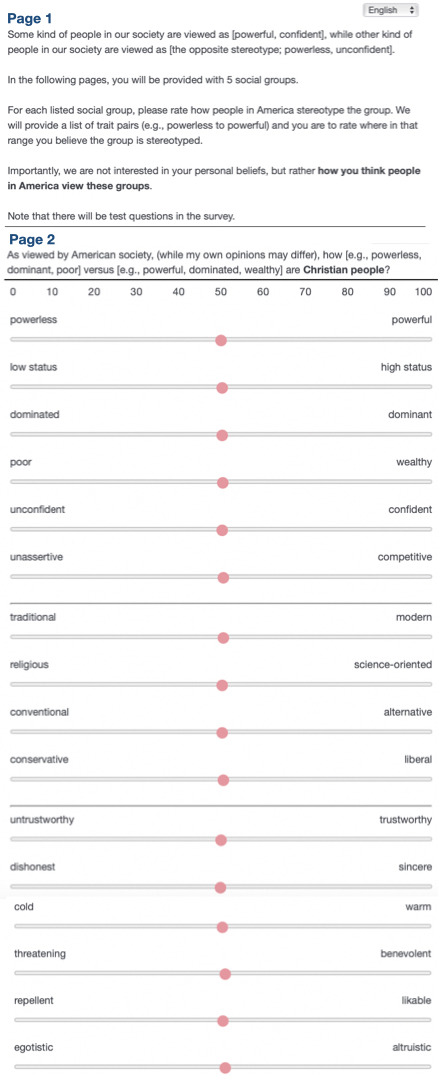
Figure A2: Example of the survey for one group.

Appendix E Annotators demographics

$55.4\%$ are white, with $50.6\%$ male annotators, $40.4$ female annotators and no annotators who provided another gender. $15.1\%$ of annotators are Black, and $25.6\%$ are Hispanic with slightly more female annotators $56.4\%$. We provide four tables A14, A15, A16, A17 showing how perceptions of White people, Black people, White men, and White women are different from each other across annotator demographics. We see variations between in-group and out-group annotations. For instance, women see themselves as more powerful than men see women. While overall scores for men and women groups are similar across white and Black annotators. In Table A18, we show correlation scores for all social groups and overall score between the model and Black, white, white female, and white male annotators.

	Social Group
Trait pair	Women	Men	White	Black
powerless-powerful	46.8	81.4	80.7	37.1
low status-high status	44.9	76.3	78.6	25.5
dominated-dominant	34.3	84.8	72.6	26.3
poor-wealthy	55.2	67.7	76.6	28.8
unconfident-confident	57.3	78.3	77.4	54.7
unassertive-competitive	53.8	75.5	79.3	49.9
traditional-modern	61.8	53.3	60.8	31.7
religious-science oriented	59.9	56.1	52.8	27.0
conventional-alternative	55.3	46.7	47.1	44.2
conservative-liberal	61.7	40.8	43.0	56.8
untrustworthy-trustworthy	52.2	50.9	58.2	29.9
dishonest-sincere	52.4	45.3	56.6	37.4
cold-warm	53.8	42.3	56.8	53.0
threatening-benevolent	64.3	39.7	54.2	31.4
repellent-likable	65.5	59.7	59.1	40.3
egoistic-altruistic	50.1	42.8	50.6	47.5

Table A14: Group-trait associations from white annotators for a subset of social groups. Scores which are closer to $0$ indicate closer to the trait on the left (powerless, low status, etc.) and scores closer to $100$ indicate closer to the trait on the right (powerful, high status, etc.).

	Social Group
Trait pair	Women	Men	White	Black
powerless-powerful	61.0	93.0	73.8	56.6
low status-high status	67.8	86.0	74.3	49.3
dominated-dominant	56.0	94.0	72.5	55.3
poor-wealthy	59.0	91.0	76.8	40.6
unconfident-confident	82.3	85.0	69.7	75.9
unassertive-competitive	54.0	57.0	80.5	76.3
traditional-modern	64.8	67.0	80.3	53.7
religious-science oriented	35.5	65.0	81.8	21.7
conventional-alternative	66.0	62.0	52.5	57.9
conservative-liberal	71.3	82.0	71.5	67.7
untrustworthy-trustworthy	78.5	57.0	62.8	46.9
dishonest-sincere	78.5	61.0	62.3	42.7
cold-warm	87.5	66.0	50.7	58.3
threatening-benevolent	78.3	38.0	35.5	49.7
repellent-likable	85.0	59.0	49.3	62.1
egoistic-altruistic	80.8	77.0	59.8	39.6

Table A15: Group-trait associations from Black annotators for a subset of social groups. Scores which are closer to $0$ indicate closer to the trait on the left (powerless, low status, etc.) and scores closer to $100$ indicate closer to the trait on the right (powerful, high status, etc.).

	Social Group
Trait pair	Women	Men	White	Black
powerless-powerful	37.5	80.0	81.9	29.8
low status-high status	44.0	77.0	83.4	18.3
dominated-dominant	42.0	83.3	69.8	18.0
poor-wealthy	47.0	70.5	83.0	12.5
unconfident-confident	55.5	75.5	81.6	51.0
unassertive-competitive	61.0	83.3	82.3	39.0
traditional-modern	59.5	59.3	76.8	26.3
religious-science oriented	46.0	62.5	61.3	21.5
conventional-alternative	51.0	55.0	64.6	42.3
conservative-liberal	54.0	36.7	55.1	53.0
untrustworthy-trustworthy	49.5	45.7	47.5	32.5
dishonest-sincere	48.0	42.5	52.5	34.0
cold-warm	50.0	43.0	55.6	48.0
threatening-benevolent	56.5	34.0	48.3	24.0
repellent-likable	50.5	57.3	57.0	40.5
egoistic-altruistic	51.5	44.8	47.6	53.8

Table A16: Group-trait associations from white male annotators for a subset of social groups. Scores which are closer to $0$ indicate closer to the trait on the left (powerless, low status, etc.) and scores closer to $100$ indicate closer to the trait on the right (powerful, high status, etc.).

	Social Group
Trait pair	Women	Men	White	Black
powerless-powerful	48.1	82.8	81.8	41.3
low status-high status	45.1	75.5	76.8	29.6
dominated-dominant	33.2	86.2	78.1	31.0
poor-wealthy	56.4	64.8	73.5	38.1
unconfident-confident	57.5	81.7	76.2	56.9
unassertive-competitive	52.8	67.7	78.9	56.9
traditional-modern	62.1	47.2	51.0	34.9
religious-science oriented	58.5	49.7	50.6	30.2
conventional-alternative	55.9	38.3	37.4	45.3
conservative-liberal	62.8	45.0	38.6	59.0
untrustworthy-trustworthy	52.6	56.2	61.0	28.4
dishonest-sincere	53.1	48.2	53.9	39.1
cold-warm	54.3	41.7	51.4	55.9
threatening-benevolent	65.4	45.3	53.4	35.6
repellent-likable	67.7	62.0	53.3	40.1
egoistic-altruistic	49.9	40.7	47.7	44.0

Table A17: Group-trait associations from white female annotators for a subset of social groups. Scores which are closer to $0$ indicate closer to the trait on the left (powerless, low status, etc.) and scores closer to $100$ indicate closer to the trait on the right (powerful, high status, etc.).

	Social Group
Trait pair	Black	White	White Men	White Women
White person	​​-0.130	0.080	​​-0.180	0.220
Hispanic person	0.360	0.470	0.200	0.570
Asian person	0.560	0.100	0.190	0.050
Black person	0.470	0.370	0.250	0.370
immigrant	0.010	0.420	0.300	0.420
man	​​-0.130	0.220	0.180	0.320
woman	​​-0.060	​​-0.030	0.080	​​-0.080
wealthy person	​​-0.600	0.050	0.050	0.080
Jewish person	0.020	​​-0.020	​​-0.120	0.070
Muslim person	——	0.230	0.140	0.280
Christian	0.270	0.390	0.280	0.010
cis person	​​-0.840	0.090	​​-0.020	0.170
trans person	0.190	0.150	0.180	0.120
working class person	0.010	0.290	0.290	0.220
non-binary	​​-0.040	0.050	​​-0.030	0.120
Native American	0.140	0.070	0.080	0.130
Buddhist	0.230	0.320	0.250	0.320
Mormon	​​-0.030	0.030	0.100	​​-0.180
veteran	0.220	0.200	0.180	0.190
unemployed person	0.030	0.020	​​-0.040	0.000
teenager	0.200	0.200	0.220	0.130
elderly person	0.540	0.650	0.710	0.620
blind person	0.226	0.217	0.217	0.217
autistic person	0.267	0.217	0.267	0.167
neurodivergent person	0.092	0.050	0.092	0.033
overall	0.151	0.187	0.177	0.164

Table A18: Correlation scores between the model and white, Black, white male, and white female annotators. Scores with p-values less than $0.05$ are marked bold.

	CEAT		ILPS		ILPS⋆		SeT
	RoBERTa	BERT	RoBERTa	BERT	RoBERTa	BERT	RoBERTa	BERT
Kendall’s $\tau$	0.028	0.123$\dagger$	0.142$\dagger$	0.071	0.173$\dagger$	​​-0.007	0.174$\dagger$	0.093

Table A19: Overall alignment scores with human annotations with only test groups. The highest scores are bold for each row. For correlation scores, we mark scores where the p-value is $<0.05$ with $\dagger$.

References

- Abele et al. (2020) Andrea Abele, Naomi Ellemers, Susan Fiske, Alex Koch, and Vincent Yzerbyt. 2020. Navigating the social world: Toward an integrated framework for evaluating self, individuals, and groups. Psychological review, 128.
- Abele and Wojciszke (2014) Andrea Abele and Bogdan Wojciszke. 2014. Communal and agentic content a dual perspective model. Adv. Exp. Soc. Psychol., 50:198–255.
- Bender et al. (2021) Emily M Bender, Timnit Gebru, Angelina McMillan-Major, and Shmargaret Shmitchell. 2021. On the dangers of stochastic parrots: Can language models be too big? In Proceedings of the 2021 ACM Conference on Fairness, Accountability, and Transparency, pages 610–623.
- Beygelzimer et al. (2008) Alina Beygelzimer, Sanjoy Dasgupta, and John Langford. 2008. Importance weighted active learning. CoRR, abs/0812.4952.
- Bittorf et al. (2012) Victor Bittorf, Benjamin Recht, Christopher Ré, and Joel Tropp. 2012. Factoring nonnegative matrices with linear programs. Advances in Neural Information Processing Systems, 2.
- Blodgett et al. (2021) Su Lin Blodgett, Gilsinia Lopez, Alexandra Olteanu, Robert Sim, and Hanna Wallach. 2021. Stereotyping Norwegian salmon: An inventory of pitfalls in fairness benchmark datasets. In Proceedings of the 59th Annual Meeting of the Association for Computational Linguistics and the 11th International Joint Conference on Natural Language Processing (Volume 1: Long Papers), pages 1004–1015, Online. Association for Computational Linguistics.
- Bolukbasi et al. (2016) Tolga Bolukbasi, Kai-Wei Chang, James Zou, Venkatesh Saligrama, and Adam Kalai. 2016. Man is to computer programmer as woman is to homemaker? debiasing word embeddings. NeurIPS, pages 4349–4357.
- Bonilla-Silva (1997) Eduardo Bonilla-Silva. 1997. Rethinking racism: Toward a structural interpretation. American sociological review, pages 465–480.
- Botsch (2011) Robert E. Botsch. 2011. Significance and Measures of Association.
- Browne and Misra (2003) Irene Browne and Joya Misra. 2003. The intersection of gender and race in the labor market. Annual review of sociology, 29(1):487–513.
- Bruner et al. (1957) J.S. Bruner, Brunswik E, L. Festinger, F. Heider, K.F. Muenzinger, C.E. Osgood, and D. Rapaport. 1957. Going beyond the information given. Contemporary approaches to cognition, pages 41–67.
- Caliskan et al. (2017) Aylin Caliskan, Joanna J Bryson, and Arvind Narayanan. 2017. Semantics derived automatically from language corpora contain human-like biases. Science, 356(6334):183–186.
- Cao et al. (2022) Yang Trista Cao, Yada Pruksachatkun, Kai-Wei Chang, Rahul Gupta, Varun Kumar, Jwala Dhamala, and Aram Galstyan. 2022. On the intrinsic and extrinsic fairness evaluation metrics for contextualized language representations.
- Collins (2002) Patricia Hill Collins. 2002. Black feminist thought: Knowledge, consciousness, and the politics of empowerment. routledge.
- Combahee River Collective (1977) Combahee River Collective. 1977. A Black Feminist Statement. na.
- Combahee River Collective (1983) Combahee River Collective. 1983. The combahee river collective statement. Home girls: A Black feminist anthology, 1:264–274.
- Crenshaw (1989) Kimberlé Crenshaw. 1989. Demarginalizing the intersection of race and sex: A black feminist critique of antidiscrimination doctrine, feminist theory and antiracist politics. u. Chi. Legal f., page 139.
- Daumé and Kumar (2017) Hal Daumé, III and Abhishek Kumar. 2017. Column squishing for multiclass updates (blog post).
- Devlin et al. (2019) Jacob Devlin, Ming-Wei Chang, Kenton Lee, and Kristina Toutanova. 2019. Bert: Pre-training of deep bidirectional transformers for language understanding. In NAACL-HLT (1).
- Ellemers (2017) Naomi Ellemers. 2017. Morality and the Regulation of Social Behavior: Groups as Moral Anchors.
- Fiske et al. (2002) Susan T. Fiske, Amy J. C. Cuddy, Peter Glick, and Jun Xu. 2002. A model of (often mixed) stereotype content: competence and warmth respectively follow from perceived status and competition. Journal of personality and social psychology, 82 6:878–902.
- Gebru et al. (2018) Timnit Gebru, Jamie Morgenstern, Briana Vecchione, Jennifer Wortman Vaughan, Hanna Wallach, Hal Daumé, and Kate Crawford. 2018. Datasheets for datasets.
- Ghavami and Peplau (2013) Negin Ghavami and Letitia Anne Peplau. 2013. An intersectional analysis of gender and ethnic stereotypes: Testing three hypotheses. Psychology of Women Quarterly, 37(1):113–127.
- Guo and Caliskan (2021) Wei Guo and Aylin Caliskan. 2021. Detecting emergent intersectional biases: Contextualized word embeddings contain a distribution of human-like biases. In Proceedings of the 2021 AAAI/ACM Conference on AI, Ethics, and Society, AIES ’21, page 122–133, New York, NY, USA. Association for Computing Machinery.
- Hazen et al. (2020) Timothy J. Hazen, Alexandra Olteanu, Gabriella Kazai, Fernando Diaz, and Michael Golebiewski. 2020. On the social and technical challenges of web search autosuggestion moderation. arXiv:2007.05039 [cs]. ArXiv: 2007.05039.
- hooks (1992) bell hooks. 1992. Yearning: Race, gender, and cultural politics. Hypatia, 7(2).
- Hovy and Yang (2021) Dirk Hovy and Diyi Yang. 2021. The importance of modeling social factors of language: Theory and practice. In Proceedings of the 2021 Conference of the North American Chapter of the Association for Computational Linguistics: Human Language Technologies, pages 588–602, Online. Association for Computational Linguistics.
- Jackson (2011) Lynne M. Jackson. 2011. The psychology of prejudice: From attitudes to social action. American Psychological Association.
- King (1988) Deborah K King. 1988. Multiple jeopardy, multiple consciousness: The context of a black feminist ideology. Signs: Journal of women in culture and society, 14(1):42–72.
- Koch et al. (2016) Alex Koch, Roland Imhoff, Ron Dotsch, Christian Unkelbach, and Hans Alves. 2016. The abc of stereotypes about groups: Agency/socioeconomic success, conservative-progressive beliefs, and communion. Journal of personality and social psychology, 110:675–709.
- Koch et al. (2021) Alex Koch, Vincent Yzerbyt, Andrea Abele, Naomi Ellemers, and Susan T. Fiske. 2021. Social evaluation: Comparing models across interpersonal, intragroup, intergroup, several-group, and many-group contexts, volume 63, page 1–68. Elsevier.
- Kurita et al. (2019) Keita Kurita, Nidhi Vyas, Ayush Pareek, Alan W. Black, and Yulia Tsvetkov. 2019. Measuring bias in contextualized word representations. CoRR, abs/1906.07337.
- Latkin et al. (2017) Carl A. Latkin, Catie Edwards, Melissa A. Davey-Rothwell, and Karin E. Tobin. 2017. The relationship between social desirability bias and self-reports of health, substance use, and social network factors among urban substance users in baltimore, maryland. Addictive Behaviors, 73:133–136.
- Lippmann (1965) Walter Lippmann. 1965. Public Opinion. New York :Free Press.
- Liu et al. (2019) Yinhan Liu, Myle Ott, Naman Goyal, Jingfei Du, Mandar Joshi, Danqi Chen, Omer Levy, Mike Lewis, Luke Zettlemoyer, and Veselin Stoyanov. 2019. RoBERTa: A robustly optimized bert pretraining approach. arXiv preprint arXiv:1907.11692.
- May et al. (2019) Chandler May, Alex Wang, Shikha Bordia, Samuel R. Bowman, and Rachel Rudinger. 2019. On measuring social biases in sentence encoders. In Proceedings of the 2019 Conference of the North American Chapter of the Association for Computational Linguistics: Human Language Technologies, Volume 1 (Long and Short Papers), pages 622–628, Minneapolis, Minnesota. Association for Computational Linguistics.
- Nadeem et al. (2020) Moin Nadeem, Anna Bethke, and Siva Reddy. 2020. Stereoset: Measuring stereotypical bias in pretrained language models. CoRR, abs/2004.09456.
- Nangia et al. (2020) Nikita Nangia, Clara Vania, Rasika Bhalerao, and Samuel R. Bowman. 2020. CrowS-pairs: A challenge dataset for measuring social biases in masked language models. In Proceedings of the 2020 Conference on Empirical Methods in Natural Language Processing (EMNLP), pages 1953–1967, Online. Association for Computational Linguistics.
- Nozza et al. (2021) Debora Nozza, Federico Bianchi, and Dirk Hovy. 2021. HONEST: Measuring hurtful sentence completion in language models. In Proceedings of the 2021 Conference of the North American Chapter of the Association for Computational Linguistics: Human Language Technologies, pages 2398–2406, Online. Association for Computational Linguistics.
- Paun et al. (2018) Silviu Paun, Bob Carpenter, Jon Chamberlain, Dirk Hovy, Udo Kruschwitz, and Massimo Poesio. 2018. Comparing Bayesian Models of Annotation. Transactions of the Association for Computational Linguistics, 6:571–585.
- Sap et al. (2019) Maarten Sap, Saadia Gabriel, Lianhui Qin, Dan Jurafsky, Noah A. Smith, and Yejin Choi. 2019. Social bias frames: Reasoning about social and power implications of language. CoRR, abs/1911.03891.
- Sotnikova et al. (2021) Anna Sotnikova, Yang Trista Cao, Hal Daumé III, and Rachel Rudinger. 2021. Analyzing stereotypes in generative text inference tasks. In Findings of the Association for Computational Linguistics: ACL-IJCNLP 2021, pages 4052–4065, Online. Association for Computational Linguistics.
- Stangor (2014) Dr. Charles Stangor. 2014. Principles of social psychology – 1st international edition. BCcampus.
- Steinbugler et al. (2006) Amy C Steinbugler, Julie E Press, and Janice Johnson Dias. 2006. Gender, race, and affirmative action: Operationalizing intersectionality in survey research. Gender & Society, 20(6):805–825.
- Stryker (1980) Sheldon Stryker. 1980. Symbolic interactionism: a social structural version. Benjamin/Cummings Pub. Co.
- Wheeler and Petty (2001) S. Wheeler and Richard Petty. 2001. The effects of stereotype activation on behavior: A review of possible mechanisms. Psychological bulletin, 127:797–826.
- Wod (1985) I.J. Wod. 1985. Weight of evidence: A brief survey. Bayesian statistics, 2:249–270.
- Yzerbyt (2018) Vincent Y. Yzerbyt. 2018. The dimensional compensation model. Agency and Communion in Social Psychology.
- Zinn and Dill (1996) Maxine Baca Zinn and Bonnie Thornton Dill. 1996. Theorizing difference from multiracial feminism. Feminist studies, 22(2):321–331.