Capacity Optimality of OAMP in Coded Large Unitarily Invariant Systems

Abstract

This paper investigates a large unitarily invariant system (LUIS) involving a unitarily invariant sensing matrix, an arbitrary fixed signal distribution, and forward error control (FEC) coding. Several area properties are established based on the state evolution of orthogonal approximate message passing (OAMP) in an un-coded LUIS. Under the assumptions that the state evolution for joint OAMP and FEC decoding is correct and the replica method is reliable, we analyze the achievable rate of OAMP. We prove that OAMP reaches the constrained capacity predicted by the replica method of the LUIS with an arbitrary signal distribution based on matched FEC coding. Meanwhile, we elaborate a constrained capacity-achieving coding principle for LUIS, based on which irregular low-density parity-check (LDPC) codes are optimized for binary signaling in the simulation results. We show that OAMP with the optimized codes has significant performance improvement over the un-optimized ones and the well-known Turbo linear MMSE algorithm. For quadrature phase-shift keying (QPSK) modulation, constrained capacity-approaching bit error rate (BER) performances are observed under various channel conditions.

A full version of this paper is accessible at arXiv (see [1]).

I Introduction

Consider estimating $\bm{x}=\{x_{i}\}\in\mathbb{C}^{N}$ from its observation $\bm{y}\in\mathbb{C}^{M}$ in a linear system

$$\bm{y}=\bm{Ax}+\bm{n},\vspace{-1mm}$$ (1)

where $\bm{n}\in\mathbb{C}^{M}$ contains Gaussian noise samples. For convenience, we refer to $\bm{A}\in\mathbb{C}^{M\times N}$ as a sensing matrix. We assume that $\{x_{i}\}$ follow a fixed distribution $x_{i}\sim P_{X},\forall i$. Furthermore, we assume that $\bm{x}$ is generated by a forward error control (FEC) code that includes un-coded $\bm{x}$ as a special case.

A wide range of communication applications can be modeled by (1). A classic one is a multiple-input multiple-output (MIMO) system where $\bm{A}$ is a channel coefficient matrix [2, 3] and $P_{X}$ is determined by the signaling (i.e., modulation) method. Continuous Gaussian signaling, with which $\{x_{i}\}$ are independently and identically distributed (IID) Gaussian (IIDG), is often assumed in information theoretical studies but, due to implementation concerns, all practically used signaling methods are discrete such as quadrature phase-shift keying (QPSK).

A more recent application of (1) is the so-called massive-access scheme where $\bm{A}$ consists of pilot signals and $P_{X}$ is jointly determined by channel coefficients and user activity [4, 5]. In this case, a common assumption of $P_{X}$ is Bernoulli-Gaussian. Massive-access has attracted wide research interests for machine-type communications in the $5^{\rm th}$ and $6^{\rm th}$ generation (5G and 6G) cellular systems.

Two performance measures are commonly used for the system in (1), namely mean squared error (MSE) for an un-coded system and achievable rate for a FEC coded one. The optimal limits in these two cases are respectively given by minimum MSE (MMSE) and information theoretic capacity. For simplicity, we say that a receiver is MMSE-optimal if its MSE achieves MMSE for un-coded $\bm{x}$, or capacity-optimal if its achievable rate reaches mutual information $I(\bm{x};\bm{y})$ for coded $\bm{x}$. Optimal receivers under both measures generally have prohibitively high complexity [6, 7] except for a few cases listed below.

• The classic linear MMSE (LMMSE) detector is optimal when (1) is un-coded with IIDG signaling [8].

• Some compressed-sensing algorithms are asymptotically MMSE-optimal when $\bm{x}$ is un-coded and sparse.

• When $\bm{A}$ is diagonal, (1) is equivalent to a set of parallel single-input-single-output (SISO) sub-systems. Turbo [9, 10] or low-density parity-check (LDPC) [11, 12] codes are nearly capacity-optimal in this case.

• For Gaussian signaling, Turbo-type detection algorithms [13] are capacity-optimal using proper coding [14, 15, 16].

For discrete signaling with dense $\bm{A}$ and $\bm{x}$, however, detection with proven MMSE/capacity optimality and practical complexity remained a difficult issue until recently [19, 20, 21, 17, 18, 22].

Approximate message passing (AMP) represents a remarkable progress measured by both types of optimality with practical complexity. AMP employs a so-called Onsager term to regulate the correlation problem in iterative processing [23]. A distinguished feature of AMP is that its asymptotic MSE performance can be accurately analyzed by a state-evolution (SE) technique [24]. Based on SE, the MMSE optimality of AMP is proved in [17, 18]. The capacity optimality of AMP is proved in [22].

We will say that $\bm{A}$ in (1) is IIDG when its entries are IIDG. Good performance of AMP is guaranteed only when $\bm{A}$ is IIDG. This IIDG restriction is relaxed in orthogonal AMP (OAMP) [25, 26, 27]. Let the singular value decomposition (SVD) of $\bm{A}$ be $\bm{A}\!=\!\bm{U}^{\rm H}\bm{\Sigma}\bm{V}$, where $\bm{U}\!\in\!\mathbb{C}^{M\times M}$ and $\bm{V}\!\in\!\mathbb{C}^{N\times N}$ are unitary and $\bm{\Sigma}$ is an $M\times N$ rectangular diagonal matrix. We will say that $\bm{V}$ is Haar distributed if $\bm{V}$ is uniformly distributed over all unitary matrices [28, 29]. We will say that $\bm{A}$ is right-unitarily invariant if $\bm{V}$ is Haar distributed. We will call (1) a large unitarily invariant system (LUIS) when $M,N\to\infty$ with their ratio fixed and $\bm{V}$ is Haar distributed. Recently, to avoid the high complexity LMMSE in OAMP, low-complexity convolutional AMP (CAMP) [32] and memory AMP (MAMP) [33] were proposed for LUIS. The MMSE and constrained capacity of LUIS can be predicted by the replica method from statistical physics [21, 20]. However, the replica method involves an exchange of limits and the assumption of replica symmetry, which are unproven for general LUIS. Recently, it is proven that the MMSE and constrained capacity predicted by the replica method are correct for a sub-class of LUIS [19]. For more cases, a rigorous proof of the replica method is still open issues.

This paper concerns the capacity optimality. One of the tools used this paper is the SE technique for OAMP that is conjectured for LUIS in [25] and rigorously proved in [30, 31]. Another tool is the replica method is a major tool in our derivation. For convenience, we will call the MMSE and constrained capacity predicted by the replica method as “replica MMSE” and “replica constrained capacity”, respectively. We will say that a receiver is MMSE-optimal if its MSE achieves the replica MMSE when $\bm{x}$ is un-coded, or capacity-optimal if its achievable rate reaches the replica constrained capacity when $\bm{x}$ is coded. We will show that OAMP can achieve the constrained capacity of LUIS provided that the SE and replica methods are reliable for OAMP.

As related works, the MMSE-optimality of OAMP in LUIS was derived in [30, 31] under the assumption that the SE for OAMP is accurate. We demonstrated the capacity optimality of AMP in [22] using the I-MMSE and area properties [43, 44]. As mentioned above, AMP is most suited to systems with IIDG sensing matrices. Unitarily-invariant matrices form a larger set that includes IIDG matrices as a special case. Hence OAMP is applicable to a wider range of applications than AMP. The extension of the derivations in [22] from AMP to OAMP is not straightforward, since orthogonal local estimators are generally not (locally) MMSE-optimal, so the I-MMSE property cannot be used directly in OAMP. In this paper, we will circumvent this difficulty by properly remodeling the OAMP receiver structure.

AMP-type algorithms, including OAMP, all involve iteration between two local processors such as linear estimator (LE) $\gamma$ and non-linear estimator (NLE) $\phi$ [23, 25, 30]. The performance of these two local processors can be respectively characterized by two transfer functions $\gamma_{\rm SE}$ and $\phi_{\rm SE}$ using the SE technique [24, 31, 30]. Following [22], we call mutual information $I(\bm{x};\bm{y})$ the constrained capacity of the system in (1). We proved the capacity optimality of AMP in [22] based on the assumption of MMSE-optimal NLE $\phi$.

Unfortunately, we cannot assume the local processors in OAMP are MMSE-optimal. This is due to the requirement of input-output error orthogonality on the local processors in OAMP. MMSE-optimal processors are generally not orthogonal, so the local processors in OAMP are generally not MMSE-optimal. This constitutes a main difficulty in extending the results on AMP in [22] to OAMP. In this paper, we overcome the difficulty using an equivalent structure of OAMP such that the NLE can be MMSE-optimal. It allows the use of the mutual information-MMSE (I-MMSE) theorem to obtain the achievable rate of OAMP. We prove that this achievable rate is equal to the replica constrained capacity, which leads to the capacity optimality of OAMP. The proof of capacity optimality of OAMP in this paper can also be extended to the vector AMP algorithm (VAMP) [30] and expectation propagation (EP) [36, 35, 34] due to the algorithmic equivalence between these algorithms. Such equivalence is noted in [37, 32, 31].

OAMP is being extensively investigated in many emerging applications including MIMO channel estimation and massive access [37, 40, 38, 39] since it is not restricted to systems with Gaussian signaling, sparsity and IIDG sensing matrices. Most exiting works on OAMP are for un-coded case. The findings in this paper provide an optimization technique for coded cases.

II System Model and Preliminaries

A large unitarily invariant system (LUIS) in (1) consists of a linear constraint $\Gamma$ and a non-linear constraint $\Phi$:

$${\rm Linear\;constraint}\;\;\Gamma:\quad \bm{y}=\bm{Ax}+\bm{n},$$ (2a)

$${\rm Non\!\!-\!\!linear\;constraint}\;\;\Phi:\quad \bm{x}\sim P_{\bm{X}}(\bm{x}),$$ (2b)

where $\bm{y}\!\in\!\mathbb{C}^{M\!\times\!1}$ is an observed vector, $\bm{A}\!\in\!\mathbb{C}^{M\!\times\!N}$ a right-unitarily invariant measurement matrix and $\bm{n}\!\sim\!\mathcal{CN}(\mathbf{0},\sigma^{2}\bm{I}_{M})$ a Gaussian noise vector. The average power of $\bm{x}$ is normalized, i.e., $\frac{1}{N}\mathrm{E}\{\|{\bm{x}}\|^{2}\}=1$, and $snr=\sigma^{-2}$ is the transmit SNR. We consider a large-scale LUIS that $M,N\to\infty$ with a fixed $\beta=N/M$. Only the receiver knows $\bm{A}$. This assumption was frequently used in multiple-input-multiple-output (MIMO) communications [37, 15].

For an un-coded LUIS, the constraint (2b) can be rewritten in a symbol-by-symbol manner as:

$${\rm Constellation\;constraint}\;\;\Phi_{\cal S}:\quad x_{i}\sim P_{X}(x),\;\forall i.$$ (3)

That is, the entries of $\bm{x}$ are IID with distribution $P_{X}(x)$.

In an un-coded LUIS, mean squared error (MSE) is commonly used for performance measurement. If $P_{X}(x)$ is a Gaussian distribution, the optimal solution is the standard linear minimum MSE (MMSE) estimate. For non-Gaussian distribution $P_{X}(x)$, finding the optimal solution is generally NP hard [6, 7].

In an un-coded LUIS, an error-free estimation can not be guaranteed. To ensure an error-free estimation, we consider the LUIS with forward error control (FEC) coding. For a coded LUIS, the constraint in (2b) is rewritten to a code constraint:

$${\rm Code\;constraint}\;\;\Phi_{\cal C}:\quad\bm{x}\in\bm{\mathcal{C}}\;\;{\rm and}\;\;x_{i}\sim P_{X}(x),\;\forall i,$$ (4)

where the entries of $\bm{x}$ have the identical distribution $P_{X}(x)$.

In a coded LUIS, achievable rate is commonly used for performance metrics. For a specific receiver, the code rate $R_{\bm{\mathcal{C}}}$ of codebook $\bm{\mathcal{C}}$ is an achievable rate, if its estimation of $\bm{x}$ under code constraint $\bm{\mathcal{C}}$ is error-free, i.e., ${\rm mmse}\{\bm{x}|\bm{y},\bm{A},{\Gamma},\Phi_{\cal C}\}\equiv\tfrac{1}{N}{\mathrm{E}}\{\|{\rm E}\{\bm{x}|\bm{y},\bm{A},{\Gamma},\Phi_{\cal C}\}-{\bm{x}}\|^{2}\}\to 0$ or equivalently, the block error probability$\to 0$. A natural upper bound of achievable rate is the constrained capacity of LUIS, i.e., i.e., the mutual information given $x\sim P_{X}(x)$:

$$R_{\bm{\mathcal{C}}}\leq C_{\rm LUIS}=I(\bm{x};\bm{y}).$$ (5)

Our aim is to find a coding scheme and a receiver with practical complexity such that the achievable rate approaches the constrained capacity of LUIS, i.e., $R_{\bm{\mathcal{C}}}\to C_{\rm LUIS}$.

For arbitrary signal distributions, the constrained capacity of LUIS is not trivial and was conjectured by replica method for right-unitarily-invariant matrices in [21, 20].

Lemma 1 (Constrained Capacity)

Suppose that $\rho^{*}$ is the unique solution of $\rho^{*}=snr\,\mathcal{R}_{\bm{R}}\big{(}-snr\,v^{*}\big{)}$ where $v^{*}={\rm mmse}\{\bm{x}|\sqrt{\rho^{*}}\bm{x}+\bm{z},\Phi\}$ denotes the replica MMSE of a LUIS [21, 20, 19]. The constrained capacity of a LUIS predicted by replica method [21, 20, 19] is given by

$$C^{\rm Rep}_{\rm LUIS}(snr)\!=\!\!\!\int_{0}^{v^{*}\!snr}\!\!\!\mathcal{R}_{\bm{R}}(-z)dz+I(x;\sqrt{\rho^{*}}x+z)-\rho^{*}v^{*},$$ (6)

where $z\sim\mathcal{CN}(0,1)$, and $\mathcal{R}_{\bm{R}}(\cdot)$ is the R-transform of matrix $\bm{R}=\bm{A}^{H}\bm{A}$ (see [29] for an introduction to this transform).

Since the replica method is heuristic, the exact constrained capacity of LUIS is still an open issue. Recently, the replica results were justified in [19] for a sub-class of right-unitarily-invariant matrices $\bm{A}=\bm{U}\bm{W}$, where $\bm{W}$ is IIDG, $\bm{U}$ is a product of a finite number of independent matrices, each with IID matrix-elements that are either bounded or standard Gaussian, and $\bm{U}$ and $\bm{W}$ are independent.

How to design a coding scheme and a receiver with practical complexity to achieve the replica constrained capacity is still an open issue. In this paper, we will prove the capacity optimality of OAMP based on a matching principle.

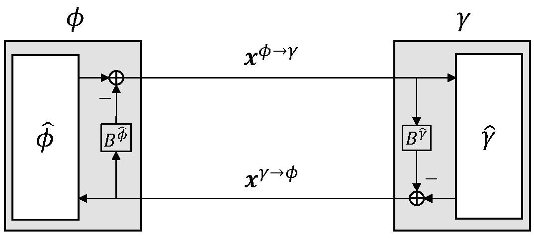
Figure 1: Graphical illustration for OAMP receiver involving two local orthogonal estimators $\gamma$ (for $\Gamma$) and $\phi$ (for $\Phi$) , which are constructed by GSO based on the prototypes $\hat{\gamma}$ and $\hat{\phi}$, respectively.

III Orthogonal AMP (OAMP)

In this paper, we consider locally optimal prototypes:

$${\rm LE:}\quad\hat{\gamma}_{t}\big{(}\bm{x}^{\phi\to\gamma}_{t}\big{)} ={\rm E}\{\bm{x}|\bm{x}^{\phi\to\gamma}_{t},\Gamma\},$$ (7a)

$${\rm NLE:}\quad\hat{\phi}_{t}\big{(}\bm{x}^{\gamma\to\phi}_{t}\big{)} ={\rm E}\{\bm{x}|\bm{x}^{\gamma\to\phi}_{t},\Phi\}.$$ (7b)

Let the messages be in Gram-Schmidt (GS) models [1]:

$$\bm{x}^{\phi\to\gamma}_{t}=\alpha_{t}^{\phi\to\gamma}\bm{x}+\bm{\xi}_{t}^{\phi\to\gamma},\quad\bm{x}^{\gamma\to\phi}_{t}=\alpha_{t}^{\gamma\to\phi}\bm{x}+{\bm{\xi}}^{\gamma\to\phi}_{t}.$$ (8)

Let the average powers of the GS errors $\bm{\xi}_{t}^{\phi\to\gamma}$ and ${\bm{\xi}}^{\gamma\to\phi}_{t}$ be $v^{\phi\to\gamma}$ and $v^{\gamma\to\phi}_{t}$, respectively. OAMP can be constructed as

$$\bm{x}^{\gamma\to\phi}_{t} ={\gamma}_{t}\big{(}\bm{x}^{\phi\to\gamma}_{t}\big{)}=\hat{\gamma}_{t}\big{(}\bm{x}^{\phi\to\gamma}_{t}\big{)}-B_{\hat{\gamma}_{t}}\bm{x}^{\phi\to\gamma}_{t},$$ (9a)

$$\bm{x}^{\phi\to\gamma}_{t+1} ={\phi}_{t}\big{(}\bm{x}^{\gamma\to\phi}_{t}\big{)}=\hat{\phi}_{t}\big{(}\bm{x}^{\gamma\to\phi}_{t}\big{)}-B_{\hat{\phi}_{t}}\bm{x}^{\gamma\to\phi}_{t},$$ (9b)

where $B_{\hat{\gamma}_{t}}$ and $B_{\hat{\phi}_{t}}$ are GS coefficients given by

$$B_{\hat{\gamma}_{t}}=\mathrm{E}\{(\bm{\xi}^{\phi\to\gamma}_{t})^{\mathrm{H}}\hat{\gamma}_{t}\big{(}\bm{x}^{\phi\to\gamma}_{t}\big{)}\}/\mathrm{E}\{\|\bm{\xi}^{\phi\to\gamma}_{t}\|^{2}\},$$ (10a)

$$B_{\hat{\phi}_{t}}=\mathrm{E}\{(\bm{\xi}^{\gamma\to\phi}_{t})^{\mathrm{H}}\hat{\phi}_{t}\big{(}\bm{x}^{\gamma\to\phi}_{t}\big{)}\}/\mathrm{E}\{\|\bm{\xi}^{\gamma\to\phi}_{t}\|^{2}\}.$$ (10b)

Refer to [1] for specific calculations of the GS coefficients. Fig. 1 gives the block diagram of OAMP.

We define the true errors as $\bm{e}_{t}^{{\phi}\to\gamma}\equiv\bm{x}_{t}^{{\phi}\to\gamma}-\bm{x}$, $\bm{e}_{t}^{{\gamma}\to\phi}\equiv\bm{x}_{t}^{{\gamma}\to\phi}-\bm{x}$, $v_{t}\equiv\tfrac{1}{N}{\rm E}\big{\{}\|\bm{e}_{t}^{{\phi}\to\gamma}\|^{2}\big{\}}$ and $\rho_{t}\equiv N/{\rm E}\big{\{}\|\bm{e}_{t}^{\gamma\to{\phi}}\|^{2}\}$. The following lemma was proved in [30, 31] for OAMP in an un-coded LUIS with IID input $\bm{x}$.

Lemma 2 (Asymptotic IIDG)

Let $\bm{x}\sim\Phi_{\cal S}$ (see (3)). In OAMP, $\bm{e}_{t}^{\gamma\to{\phi}}$ can be modeled by a sequence of IIDG samples independent of $\bm{x}$. The $\gamma_{t}$ and ${\phi}_{t}$ in OAMP can be characterized by the following transfer functions:

$$\rho={\gamma}_{\rm SE}(v)\equiv[\hat{\gamma}_{\rm SE}(v)]^{-1}-v^{-1},$$ (11a)

$$v={\phi}_{\rm SE}^{\cal S}(\rho)\equiv\big{(}[\hat{\phi}_{\rm SE}^{\cal S}(\rho)]^{-1}-\rho\big{)}^{-1}.$$ (11b)

where $\hat{\gamma}_{\rm SE}(v)=\tfrac{1}{N}{\mathrm{tr}}\left\{[snr\bm{A}^{H}\bm{A}+v^{-1}\,\bm{I}]^{-1}\right\}$, $\hat{\phi}_{\rm SE}^{\cal S}(\rho)={\rm mmse}\{\bm{x}|\sqrt{\rho}\bm{x}+\bm{z},\Phi_{\cal S}\}$, $\bm{z}\sim\mathcal{CN}(\bm{0},\bm{I})$ and $\hat{\gamma}_{\rm SE}^{-1}(\cdot)$ is the inverse of $\hat{\gamma}_{\rm SE}(\cdot)$.

IV Area Properties of LUIS

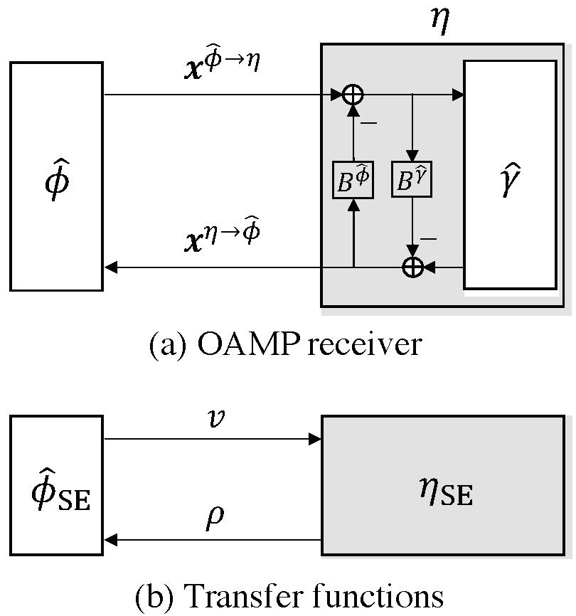
Figure 2: Graphical illustrations of OAMP receiver and the transfer functions.

The I-MMSE property derived in [43, 44] establishes a connection between achievable rate and MMSE performance. Below, we will apply this property to examine the capacity optimality of OAMP. In general, an MMSE-optimal estimator does not meet the orthogonal requirement defined in Section III. This constitutes a difficulty in directly applying the I-MMSE property to OAMP. In this subsection, we outline an equivalent structure of OAMP, which circumvents this difficulty. We rewrite the OAMP in (9) to

$$\bm{x}_{t}^{\eta\to\hat{\phi}}=\eta_{t}\big{(}\bm{x}_{t}^{\hat{\phi}\to\eta}\big{)}\quad{\rm and}\quad\bm{x}_{t+1}^{\hat{\phi}\to\eta}=\hat{\phi}_{t}\big{(}\bm{x}_{t}^{\eta\to\hat{\phi}}\big{)},$$ (12)

where $\eta_{t}$ includes $\hat{\gamma}_{t}$ and the GSO operations. Fig. 2(a) gives a graphical illustration of (12).

Let $\rho_{t}\equiv{{N}/{\rm E}\big{\{}\|\bm{x}_{t}^{\eta\to\hat{\phi}}-\bm{x}\|^{2}\}}$ and $v_{t}\equiv\tfrac{1}{N}{\rm E}\big{\{}\|\bm{x}_{t}^{\hat{\phi}\to\eta}-\bm{x}\|^{2}\big{\}}$. We then rewrite the transfer functions in (11) to

$$\rho={\eta}_{\rm SE}(v)\equiv v^{-1}-[\hat{\gamma}_{\rm SE}^{-1}(v)]^{-1}\quad{\rm and}\quad v=\hat{\phi}_{\rm SE}^{\cal S}(\rho).$$ (13)

The following properties are easy to verify.

• The fixed-point equation of $\hat{\phi}_{\rm SE}^{\cal S}(\rho)={\eta}^{-1}_{\rm SE}(\rho)$ is the same as that of ${\phi}_{\rm SE}^{\cal S}(\rho)={\gamma}^{-1}_{\rm SE}(\rho)$, where ${\eta}^{-1}_{\rm SE}(\cdot)$ and ${\gamma}^{-1}_{\rm SE}(\cdot)$ are the inverses of ${\eta}_{\rm SE}(\cdot)$ and ${\gamma}_{\rm SE}(\cdot)$, respectively.

• ${\eta}^{-1}_{\rm SE}(\rho)<\hat{\phi}_{\rm SE}^{\cal S}(\rho)$ if and only if ${\gamma}^{-1}_{\rm SE}(\rho)<{\phi}_{\rm SE}^{\cal S}(\rho)$, for $\rho\leq\rho^{*}$, where $\rho^{*}$ is the fixed point of $\hat{\phi}_{\rm SE}^{\cal S}(\rho)={\eta}^{-1}_{\rm SE}(\rho)$.

Fig. 3 provides a graphical illustration of (11).

Assumption 1

There is exactly one fixed point for $\hat{\phi}_{\rm SE}^{\cal S}(\rho)={\eta}^{-1}_{\rm SE}(\rho)$ in $\rho>0$, where ${\eta}^{-1}_{\rm SE}(\cdot)$ is the inverse of ${\eta}_{\rm SE}(\cdot)$.

It is proved that the SE of OAMP is convergent [41, 42]. Let $(\rho^{*},v^{*})$ with $v^{*}=\hat{\phi}_{\rm SE}^{\cal S}(\rho^{*})$ be the unique fixed point.

Theorem 1

Suppose that Assumption 1 holds. Then the replica constrained capacity of a LUIS given $p_{X}(x)$ is given by the area $A_{\rm ADGO}$ in Fig. 3 covered by ${\eta}_{\rm SE}^{-1}$ and $\hat{\phi}_{\rm SE}^{\cal S}$, i.e.,

$$\!\!\!C^{\rm Rep}_{\rm LUIS} =A_{\rm ADGO}=\!\!\!\int_{0}^{\rho^{*}}\!\!\!\!\!{\hat{\phi}_{\rm SE}^{\cal S}(\rho)\,d\rho}+\log v^{*}\!\!+\!{\tfrac{1}{N}\log|\bm{B}|},$$ (14a)

where $\bm{B}=\big{(}[v^{*}]^{-1}-\rho^{*}\big{)}\bm{I}+snr\bm{A}^{H}\bm{A}$.

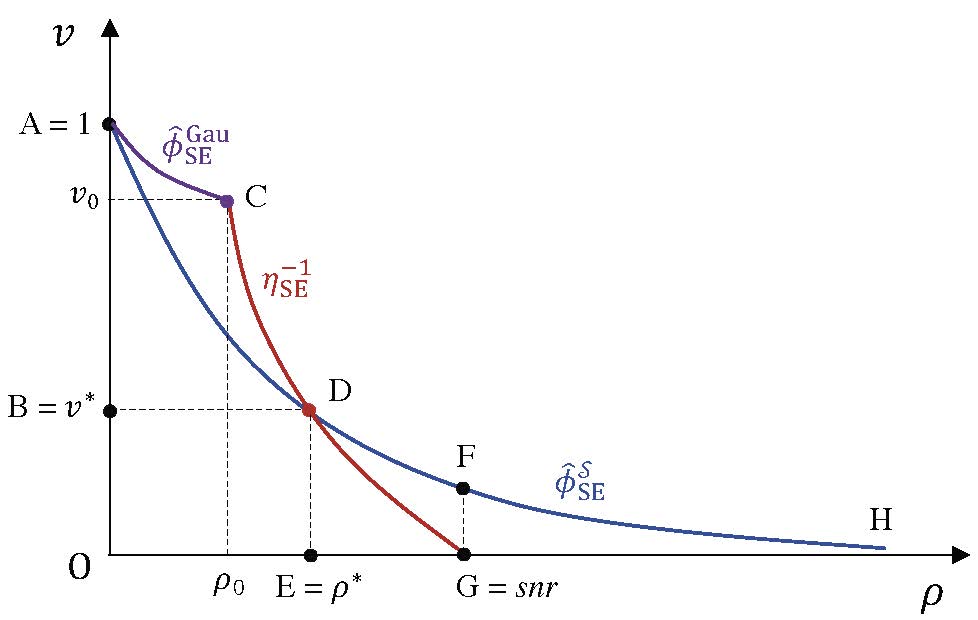
Figure 3: Graphic illustration of OAMP in the un-coded LUIS. $(\rho^{*},v^{*})$ is the fixed point of the transfer functions in (13). ${\rm H}=(0,\infty)$, $\hat{\phi}_{\rm SE}^{\rm Gau}(\rho)=1/(1+\rho)$, $\rho_{0}=[\gamma_{\rm SE}(1)]^{-1}-1$, $v_{0}=\gamma^{-1}_{\rm SE}(\rho_{0})$ and $\eta_{\rm SE}(0)=snr$.

We have the area properties below as illustrated in Fig. 3.

• Area $A_{\rm BDEO}$ is given by $A_{\rm BDEO}=\rho^{*}v^{*}$, where $(\rho^{*},v^{*})$ denotes the unique fixed point D in Fig. 3.

• Area $A_{\rm AHO}$ equals to the entropy of the constellation, i.e., $A_{\rm AHO}=\log|\mathcal{S}|$, i.e., the maximum achievable rate of a noiseless linear system in (1). See Lemma 3.

• Area $A_{\rm ADGO}$ equals to the replica constrained capacity $C^{\rm Rep}_{\rm LUIS}$ of a LUIS. See Theorem 1.

• Area $A_{\rm ACGO}$ equals to the Gaussian capacity $C_{\rm Gau}$ of a LUIS, i.e., $A_{\rm ACGO}=C_{\rm Gau}=\tfrac{1}{N}\log\det\big{(}\bm{I}+snr\bm{A}^{H}\bm{A}\big{)}$.

• Area $A_{\rm ACD}$ represents the shaping gain of Gaussian signaling. Curve AC is the Gaussian un-coded NLE.

• Area $A_{\rm ADEO}$ equals to the achievable rate of a cascading receiver with OAMP detection and decoding. That is, $A_{\rm ADEO}=R_{\rm CAS}$. There is no iteration between the OAMP detector and the decoder. Hence, the cascading receiver is not capacity optimal.

• Area $A_{\rm DGE}$ represents the rate loss for the cascading receiver, i.e., $A_{\mathrm{DGE}}=C^{\rm Rep}_{\rm LUIS}(snr)-R_{\rm CAS}(snr)$.

• Area $A_{\rm AFGO}$ equals to the constrained capacity of a SISO channel, i.e., $A_{\rm AFGO}=C_{\rm SISO}(snr)$.

• Area $A_{\rm DFG}$ represents the capacity gap of parallel SISO channels and a LUIS, i.e.,i.e., $A_{\rm DFG}=C_{\rm SISO}(snr)-C^{\rm Rep}_{\rm LUIS}(snr)$. In other words, area $A_{\rm DFG}$ represents the rate loss due to the cross-symbol interference in $\bm{Ax}$.

• Area $A_{\rm FHG}$ represents the rate loss due to the channel noise $\bm{n}$, i.e., $A_{\rm FHG}=A_{\rm AHO}-A_{\rm AFGO}$.

• Following (14), we rewrite the replica constrained capacity as $C^{\rm Rep}_{\rm LUIS}\!=\!A_{\rm BDGO}\!+\!A_{\rm ADEO}\!-\!A_{\rm BDEO}$. Since $A_{\rm BDEO}\!=\!\rho^{*}v^{*}$ and $A_{\rm ADEO}\!=\!C_{\rm SISO}(\rho^{*})\!=\!I(x;\sqrt{\rho^{*}}x+z)$, following (6), $\int_{0}^{snr\,v^{*}}\mathcal{R}_{\bm{R}}(-z)dz\!=\!A_{\rm BDGO}$.

V Achievable Rates of OAMP in Coded LUIS

For a LUIS with FEC coding, we rewrite the problem as

$${\rm Linear\;constraint}\;\;\Gamma:\quad \bm{y}=\bm{Ax}+\bm{n},$$ (15a)

$${\rm Code\;constraint}\;\;\Phi_{\cal C}:\quad \bm{x}\in\bm{\mathcal{C}},\;\;x_{i}\sim P_{X}(x),\;\forall i,$$ (15b)

where $\bm{\mathcal{C}}$ is a codebook. We focus on a joint OAMP and a-posteriori probability (APP) decoding scheme for a coded LUIS.

$$\bm{x}_{t}^{\eta\to\hat{\phi}_{\cal C}}=\eta_{t}\big{(}\bm{x}_{t}^{\hat{\phi}_{\cal C}\to\eta}\big{)},\qquad\bm{x}_{t+1}^{\hat{\phi}_{\cal C}\to\eta}=\hat{\phi}_{t}^{\cal C}\big{(}\bm{x}_{t}^{\eta\to\hat{\phi}_{\cal C}}\big{)},$$ (16)

where $\hat{\phi}_{t}^{\cal C}$ is an APP decoder for the code constraint $\bm{x}\in\bm{\mathcal{C}}$, and $\eta_{t}$ is the same as that in (12). Define

$$\bm{e}^{\hat{\phi}_{\cal C}\to\eta}_{t} \equiv\bm{x}^{\hat{\phi}_{\cal C}\to\eta}_{t}-\bm{x}, \rho_{t} \equiv\big{[}{\tfrac{1}{N}{\rm E}\big{\{}\|\bm{e}^{\hat{\phi}_{\cal C}\to\eta}_{t}\|^{2}\}}\big{]}^{-1},$$ (17a)

$$\bm{e}^{\eta\to\hat{\phi}_{\cal C}}_{t} \equiv\bm{x}^{\eta\to\hat{\phi}_{\cal C}}_{t}-\bm{x}, v_{t} \equiv\tfrac{1}{N}{\rm E}\big{\{}\|\bm{e}^{\eta\to\hat{\phi}_{\cal C}}_{t}\|^{2}\big{\}}.$$ (17b)

For coded $\bm{x}$, we make the following assumption for OAMP.

Assumption 2 (Asymptotic IIDG)

Let $\bm{x}\sim\Phi_{\cal C}$ (see (15b)). For OAMP in (16), $\eta_{t}$ and $\hat{\phi}_{t}^{\cal C}$ can be characterized by

$$\rho={\eta}_{\rm SE}(v),\quad v=\hat{\phi}_{\rm SE}^{\cal C}(\rho)\equiv{\rm mmse}\{\bm{x}|\sqrt{\rho}\bm{x}+\bm{z},\Phi_{\cal C}\},$$ (18)

where ${\eta}_{\rm SE}(\cdot)$ is the same as that in (13).

The simulation results in [37] verify that Assumption 2 hold for OAMP with convolutional codes (Fig. 4 in [37]) and LDPC codes (Fig. 7 in [37]).

V-A Curve Matching Principle

In the un-coded case, OAMP is not error-free and converges to a non-zero fixed point $(\rho^{*},v^{*})$. In the coded case, error-free recovery is possible if $\hat{\phi}_{\rm SE}^{\cal C}(\cdot)$ is properly designed. To obtain an error-free recovery, there should be no fixed point between $\hat{\phi}_{\rm SE}^{\cal C}(\rho)$ and ${\eta}_{\rm SE}^{-1}({\rho})$, which implies

$$\hat{\phi}_{\rm SE}^{\cal C}(\rho)<{\eta}_{\rm SE}^{-1}({\rho}),\;\;\;0\leq{\rho}\leq snr.$$ (19)

Also, the decoding MSE should be lower than that of the detector, i.e.,

$$\hat{\phi}_{\rm SE}^{\cal C}(\rho)<\hat{\phi}_{\rm SE}^{\cal S}(\rho),\;\;\;{\rm for}\;\;\rho\geq 0.\vspace{-0.1cm}$$ (20)

Following (19) and (20), OAMP achieves error-free recovery if and only if: For $0\leq{\rho}<snr$,

$$\hat{\phi}_{\rm SE}^{\cal C}(\rho)<\hat{\phi}_{\rm SE}^{*}(\rho)\equiv\min\{{\eta}_{\rm SE}^{-1}({\rho}),\;\hat{\phi}_{\rm SE}^{\cal S}(\rho)\}.$$ (21)

V-B Achievable Rate and Capacity Optimality of OAMP

The lemma below, proved in [44], establishes the connection between MMSE and code rate.

Lemma 3 (Code-Rate-MMSE)

Consider a code constraint $\Phi_{\cal C}:\bm{x}\in{\bm{\mathcal{C}}}$. Let the code length be $N$ and code rate $R_{\cal C}$. Then the rate of $\bm{{\mathcal{C}}}$ is given by

$$R_{\cal C}=\int_{0}^{\infty}\hat{\phi}_{\rm SE}^{\cal C}(\rho)d\rho=K/N,$$ (22)

where $\hat{\phi}_{\rm SE}^{\cal C}(\rho)\equiv\tfrac{1}{N}\mathrm{mmse}\{\bm{x}|\sqrt{\rho}\bm{x}+\bm{z},\Phi_{\bm{\mathcal{C}}}\}$ is obtained by APP decoding $\eta_{\mathcal{C}}(\sqrt{\rho}\bm{x}+\bm{z})={\rm E}\{\bm{x}|\sqrt{\rho}\bm{x}+\bm{z},\Phi_{\bm{\mathcal{C}}}\}$.

Following Lemma 3 and the error-free condition in (21), the achievable rate of OAMP receiver is given by

$$R_{\rm OAMP}(snr)=\int_{0}^{\infty}\hat{\phi}_{\rm SE}^{\cal C}(\rho)d\rho,\quad\hat{\phi}_{\rm SE}^{\cal C}(\rho)<\hat{\phi}_{\rm SE}^{*}(\rho).$$ (23)

That is, error-free detection can be achieved by the OAMP receiver if $R_{\cal C}\leq R_{\rm OAMP}$.

Theorem 2 (Capacity Optimality)

Suppose that Assumption 1 and Assumption 2 hold. Then, the achievable rate of OAMP achieves the replica constrained capacity of LUIS, i.e.,

$$R_{\rm OAMP}(snr)\to C^{\rm Rep}_{\rm LUIS}(snr),$$ (24)

if $\hat{\phi}_{\rm SE}^{\cal C}(\rho)<\hat{\phi}_{\rm SE}^{*}(\rho)$ and $\hat{\phi}_{\rm SE}^{\cal C}(\rho)\to\hat{\phi}_{\rm SE}^{*}(\rho)$ in $[0,snr]$.

For a sub-class right-unitarily-invariant $\bm{A}$, $C^{\rm Rep}_{\rm LUIS}(snr)$ is the true constrained capacity of LUIS [19]. In this case, OAMP is rigorously capacity optimal. Theorem 2 is developed under a matching constraint: $\hat{\phi}_{\rm SE}^{\cal C}(\rho)\to\hat{\phi}_{\rm SE}^{*}(\rho)$. The curve-matching code existence is proved in Appendix C-B [22] for Gaussian signaling. For non-Gaussian signaling, the curve-matching code existence is still a conjecture.

Theorem 2 is based on a matching condition $\hat{\phi}_{\rm SE}^{\cal C}(\rho)\to\hat{\phi}_{\rm SE}^{*}(\rho)$. An existence proof can be found in Appendix C-B [22] for Gaussian signaling. For other signaling, the code existence is a conjecture only.

VI Numeric Results

Let the SVD of $\bm{A}$ be $\bm{A}=\bm{U}\bm{\Sigma V}$. In all the simulations, we set the eigenvalues $\{d_{i}\}$ in $\bm{\Sigma}$ as [45]: $d_{i}/d_{i+1}=\kappa^{1/T}$ for $i=1,\ldots,T-1$ and $\sum_{i=1}^{T}d_{i}^{2}=N$, where $T=\min\{M,N\}$. Here, $\kappa\geq 1$ controls the condition number of $\bm{A}$. $\bm{U}$ and $\bm{V}$ are generated by the QR decomposition of two IIDG matrices.

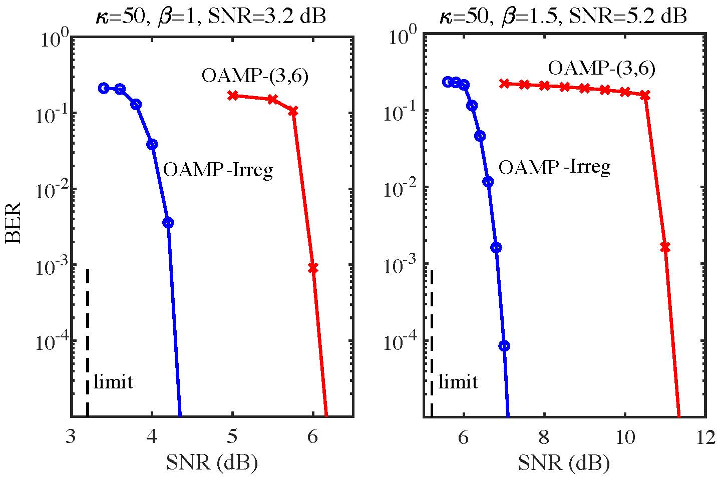
Figure 4: BER performances of OAMP , where “OAMP-Irreg” denotes the BER of optimized irregular LDPC codes, “OAMP-(3, 6)” the BER with regular (3, 6) LDPC codes. Codeword length = $10^{5}$, code rate $=$ 0.5075 (left) and 0.4721 (right), QPSK modulation, and iterations = $250$, and $\beta=N/M=\{1,1.5\}$.

Fig. 4 shows the BER simulations for the LUIS, where $\bm{x}$ is optimized irregular LDPC codes [46, 47]. The receiver “OAMP-Irreg” is shown in Fig. 1, and the NLE is a sum-product decoder. The system sizes are $(N,M)=(500,500)\;\mathrm{and}\;(500,333)$. At BER $=10^{-5}$, the curves of “OAMP-Irreg” are about $1$ dB away from their limits. We compare the “OAMP-Irreg” with “OAMP-(3, 6)”, i.e., the cascading OAMP with un-optimized regular (3, 6) LDPC codes [11]. At BER = $10^{-5}$, the proposed “OAMP-Irreg” outperforms ($0.8\sim 4$ dB gains) “OAMP-(3, 6)” for $\beta=\{1,1.5\}$ and $\kappa=\{10,50\}$. In other words, code optimization can bring significant performance improvement for OAMP.

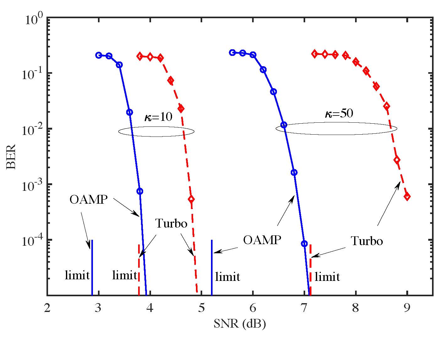
Figure 5: BER performances of OAMP and Turbo [16, 15] with optimized irregular LDPC codes, where “limit” denotes the QPSK rate limits of OAMP or Turbo. Codeword length = $10^{5}$, code rates $=\{0.5062,0.4721,0.5008,0.4863\}$ (for the curves from left to right), QPSK modulation, and iterations = $250$, and $\beta=1.5$ with $N=500$ and $M=333$.

Fig. 5 compares OAMP with the conventional Turbo [16, 15]. A QPSK modulated LUIS with $(N,M)=(500,333)$ and $\kappa=\{10,50\}$ (condition number) is considered. Fig. 5 compares the BERs of the optimized OAMP and the optimized Turbo (with iterations $=250$). The simulated BERs of OAMP and Turbo are about 1dB for $\kappa=10$ and 2 dB for $\kappa=50$ away from their limits respectively. Comparing with the Turbo, OAMP has 1 dB improvement for $\kappa=10$ and 2 dB improvement for $\kappa=50$ in BER. Overall, the conventional Turbo has huge performance loss in general discrete linear systems, especially in the case of high transmission rate and high conditional number.

VII Conclusion

An OAMP receiver is considered for a coded LUIS with a unitarily invariant sensing matrix and an arbitrary input distribution. Several area properties are established using the established properties of OAMP. We show that OAMP is capacity optimal under the assumptions that the SE for joint OAMP and FEC decoding is correct and the replica method is reliable. A curve-matching coding principle is developed for OAMP. Simulation results are provided to verify that the OAMP with optimized irregular LDPC codes approaches the replica capacity of LUIS, and significantly outperforms ($2$ dB $\sim$ $4$ dB gain) the un-optimized case. Furthermore, the OAMP has a significant improvement in BER performance over the state-of-art Turbo-LMMSE.

References

- [1] L. Liu, S. Liang, and L. Ping, “Capacity optimality of OAMP: Beyond IID sensing matrices and Gaussian signaling,” arXiv preprint: arXiv:2108.08503, Aug. 2021.
- [2] E. Biglieri, R. Calderbank, A. Constantinides, A. Goldsmith, A. Paulraj, and H. V. Poor, MIMO Wireless Communications. Cambridge, U.K.: Cambridge Univ. Press, 2007.
- [3] Tse David and P. Viswanath, Fundamentals of wireless communication. Cambridge university press, 2005.
- [4] L. Liu and W. Yu, “Massive connectivity with massive MIMO—part I: Device activity detection and channel estimation,” IEEE Trans. Signal Process., vol. 66, no. 11, pp. 2933-2946, June 2018.
- [5] L. Liu and W. Yu, “Massive connectivity with massive MIMO—part II: Achievable rate characterization,” IEEE Trans. Signal Process., vol. 66, no. 11, pp. 2947-2959, June 2018.
- [6] D. Micciancio, “The hardness of the closest vector problem with preprocessing,” IEEE Trans. Inf. Theory, vol. 47, no. 3, pp. 1212-1215, Mar. 2001.
- [7] S. Verdú, “Optimum multi-user signal detection,” Ph.D. dissertation, Department of Electrical and Computer Engineering, University of Illinois at Urbana-Champaign, Urbana, IL, Aug. 1984.
- [8] S. M. Kay, Fundamentals of Statistical Signal Processing: Estimation Theory. Upper Saddle River, NJ, USA: Prentice-Hall, 1993.
- [9] C. Berrou and A. Glavieux, “Near optimum error correcting coding and decoding: Turbo-codes,” IEEE Trans. Commun., vol. 44, no. 10, pp. 1261–1271, Oct. 1996.
- [10] C. Douillard, M. Jézéquel, C. Berrou, D. Electronique, A. Picart, P. Didier, and A. Glavieux, “Iterative correction of intersymbol interference: Turbo-equalization,” Trans. on Emerging Telecom. Techn., vol. 6, no. 5, pp. 507–511, 1995.
- [11] R. G. Gallager, “Low-density parity-check codes,” IRE Trans. Inform. Theory, vol. IT-8, pp. 21–28, Jan. 1962.
- [12] S.-Y. Chung, G. D. Forney, Jr., T. J. Richardson, and R. Urbanke, “On the design of low-density parity-check codes within 0.0045 dB of the Shannon limit,” IEEE Commun. Lett., vol. 5, pp. 58–60, Feb. 2001.
- [13] X. Wang and H. V. Poor, “Iterative (Turbo) soft interference cancellation and decoding for coded CDMA,” IEEE Trans. Commun., vol. 47, no. 7, pp. 1046–1061, Jul 1999.
- [14] X. Yuan, L. Ping, C. Xu and A. Kavcic, “Achievable rates of MIMO systems with linear precoding and iterative LMMSE detector,” IEEE Trans. Inf. Theory, vol. 60, no.11, pp. 7073-7089, Oct. 2014.
- [15] L. Liu, C. Yuen, Y. L. Guan, and Y. Li, “Capacity-achieving MIMO-NOMA: Iterative LMMSE detection,” IEEE Trans. Signal Process., vol. 67, no. 7, 1758–1773, April 2019.
- [16] Y. Chi, L. Liu, G. Song, C. Yuen, Y. L. Guan and Y. Li, “Practical MIMO-NOMA: Low complexity and capacity-approaching solution,” IEEE Trans. Wireless Commun., vol. 17, no. 9, pp. 6251-6264, Sept. 2018.
- [17] G. Reeves and H. D. Pfister, “The replica-symmetric prediction for random linear estimation with Gaussian matrices is exact,” IEEE Trans. Inf. Theory, vol. 65, no. 4, pp. 2252-2283, April 2019.
- [18] J. Barbier, N. Macris, M. Dia, and F. Krzakala, “Mutual information and optimality of approximate message-passing in random linear estimation,” IEEE Trans. Inf. Theory, vol. 66, no. 7, pp. 4270–4303, July 2020.
- [19] J. Barbier, N. Macris, A. Maillard, F. Krzakala, “The mutual information in random linear estimation beyond i.i.d. matrices,” arXiv preprint arXiv:1802.08963, 2018.
- [20] K. Takeda, S. Uda, and Y. Kabashima, “Analysis of cdma systems that are characterized by eigenvalue spectrum,” EPL (Europhysics Letters), vol. 76, no. 6, p. 1193, 2006.
- [21] A. M. Tulino, G. Caire, S. Verdú, and S. Shamai (Shitz), “Support recovery with sparsely sampled free random matrices,” IEEE Trans. Inf. Theory, vol. 59, no. 7, pp. 4243–4271, Jul. 2013.
- [22] L. Liu, C. Liang, J. Ma, and L. Ping, “Capacity optimality of AMP in coded systems”, IEEE Trans. Inf. Theory, vol. 67, no. 7, 4929-4445, July 2021.
- [23] D. L. Donoho, A. Maleki, and A. Montanari, “Message-passing algorithms for compressed sensing,” in Proc. Nat. Acad. Sci., vol. 106, no. 45, Nov. 2009.
- [24] M. Bayati and A. Montanari, “The dynamics of message passing on dense graphs, with applications to compressed sensing,” IEEE Trans. Inf. Theory, vol. 57, no. 2, pp. 764–785, Feb. 2011.
- [25] J. Ma and L. Ping, “Orthogonal AMP,” IEEE Access, vol. 5, pp. 2020–2033, 2017, preprint arXiv:1602.06509, 2016.
- [26] J. Ma, X. Yuan and L. Ping, “Turbo compressed sensing with partial DFT sensing matrix,” IEEE Signal Process. Lett., vol. 22, no. 2, pp. 158-161, Feb. 2015.
- [27] J. Ma, X. Yuan and L. Ping, “On the performance of Turbo signal recovery with partial DFT sensing matrices,” IEEE Signal Process. Lett., vol. 22, no. 10, pp. 1580-1584, Oct. 2015.
- [28] F. Hiai and D. Petz, The Semicircle Law, Free Random Variables and Entropy. Amer. Math. Soc., 2000.
- [29] A. M. Tulino and S. Verd, “Random matrix theory and wireless communications.” Commun. and Inf. theory, 2004.
- [30] S. Rangan, P. Schniter, and A. Fletcher, “Vector approximate message passing,” IEEE Trans. Inf. Theory, vol. 65, no. 10, pp. 6664-6684, Oct. 2019.
- [31] K. Takeuchi, “Rigorous dynamics of expectation-propagation-based signal recovery from unitarily invariant measurements,” IEEE Trans. Inf. Theory, vol. 66, no. 1, 368 - 386, Jan. 2020.
- [32] K. Takeuchi, “Bayes-optimal convolutional AMP,” IEEE Trans. Inf. Theory, vol. 67, no. 7, pp. 4405-4428, July 2021.
- [33] L. Liu, S. Huang, and B. M. Kurkoski, “Memory approximate message passing,” Proc. 2021 IEEE Int. Symp. Inf. Theory, pp.1379-1384, Melbourne, Australia, July 2021, arXiv preprint arXiv:2012.10861, Dec. 2020.
- [34] T. P. Minka, “Expectation propagation for approximate bayesian inference,” in Proceedings of the Seventeenth conference on Uncertainty in artificial intelligence, 2001, pp. 362–369.
- [35] M. Opper and O. Winther, “Expectation consistent approximate inference,” Journal of Machine Learning Research, vol. 6, no. Dec, pp. 2177–2204, 2005.
- [36] B. Çakmak and M. Opper, “Expectation propagation for approximate inference: Free probability framework,” arXiv preprint arXiv:1801.05411, 2018.
- [37] J. Ma, L. Liu, X. Yuan and L. Ping, ”On orthogonal AMP in coded linear vector systems,” IEEE Trans. Wireless Commun., vol. 18, no. 12, pp. 5658-5672, Dec. 2019.
- [38] M. Khani, M. Alizadeh, J. Hoydis and P. Fleming, “Adaptive neural signal detection for massive MIMO,” IEEE Trans. Wireless Commun., vol. 19, no. 8, pp. 5635-5648, Aug. 2020,
- [39] J. Zhang, H. He, C. Wen, S. Jin and G. Y. Li, “Deep learning based on orthogonal approximate message passing for CP-Free OFDM,” IEEE International Conference on Acoustics, Speech and Signal Processing (ICASSP), 2019, pp. 8414-8418,
- [40] Y Cheng, L. Liu and L. Ping, “Orthogonal AMP for massive access in channels with spatial and temporal correlations” IEEE J. Sel. Areas Commun., vol. 39, no. 3, 726-740, March 2021.
- [41] K. Takeuchi, “On the convergence of orthogonal/vector AMP: Long-memory message-passing strategy,” arXiv preprint: arXiv:2111.05522, 2021.
- [42] L. Liu, S. Huang, and B. M. Kurkoski, ‘Sufficient statistic memory AMP,” arXiv preprint: arXiv:2112.15327, Jan. 2022.
- [43] D. Guo, S. Shamai, and S. Verdú, “Mutual information and minimum mean-square error in Gaussian channels,” IEEE Trans. Inf. Theory, vol. 51, no. 4, pp. 1261-1282, Apr. 2005.
- [44] K. Bhattad and K. R. Narayanan, “An MSE-based transfer chart for analyzing iterative decoding schemes using a Gaussian approximation,” IEEE Trans. Inf. Theory, vol. 53, no. 1, pp. 22-38, Jan. 2007.
- [45] J. Vila, P. Schniter, S. Rangan, F. Krzakala, and L. Zdeborová, “Adaptive damping and mean removal for the generalized approximate message passing algorithm,” in Acoustics, Speech and Signal Processing (ICASSP), 2015 IEEE International Conference on, 2015, pp. 2021–2025.
- [46] X. Yuan, Low-complexity iterative detection in coded linear systems, PhD thesis, City University of Hong Kong, Hong Kong, China, 2008.
- [47] S.-Y. Chung, T. Richardson, and R. Urbanke, “Analysis of sum-product decoding of low-density parity-check codes using a Gaussian approximation,” vol. 47, no. 2, pp. 657–670, Feb. 2001.