plingo: A system for probabilistic reasoning in clingo based on lpmln

Abstract

We present plingo, an extension of the ASP system clingo with various probabilistic reasoning modes. Plingo is centered upon $\mathit{LP}^{\mathit{MLN}}$, a probabilistic extension of ASP based on a weight scheme from Markov Logic. This choice is motivated by the fact that the core probabilistic reasoning modes can be mapped onto optimization problems and that $\mathit{LP}^{\mathit{MLN}}$ may serve as a middle-ground formalism connecting to other probabilistic approaches. As a result, plingo offers three alternative frontends, for $\mathit{LP}^{\mathit{MLN}}$, P-log, and ProbLog. The corresponding input languages and reasoning modes are implemented by means of clingo’s multi-shot and theory solving capabilities. The core of plingo amounts to a re-implementation of $\mathit{LP}^{\mathit{MLN}}$ in terms of modern ASP technology, extended by an approximation technique based on a new method for answer set enumeration in the order of optimality. We evaluate plingo’s performance empirically by comparing it to other probabilistic systems.

1 Introduction

Answer Set Programming (ASP; [14]) offers a rich knowledge representation language along with powerful solving technology. In the last years, several probabilisitic extensions of ASP have been proposed, among them $\mathit{LP}^{\mathit{MLN}}$ [11], ProbLog [16], and P-log [3].

In this work, we present an extension of the ASP system clingo, called plingo, that features various probabilistic reasoning modes. Plingo is centered on $\mathit{LP}^{\mathit{MLN}}$, a probabilistic extension of ASP based upon a weight scheme from Markov Logic [17]. $\mathit{LP}^{\mathit{MLN}}$ has already proven to be useful in several settings [12, 1] and it serves us also as a middle-ground formalism connecting to other probabilistic approaches. We rely on translations from ProbLog and P-log to $\mathit{LP}^{\mathit{MLN}}$ [11, 13], respectively, to capture these approaches as well. In fact, $\mathit{LP}^{\mathit{MLN}}$ has already been implemented in the system lpmln2asp [10] by mapping $\mathit{LP}^{\mathit{MLN}}$-based reasoning into reasoning modes in clingo (viz. optimization and enumeration of stable models). As such, plingo can be seen as a re-implementation of lpmln2asp that is well integrated with clingo by using its multi-shot and theory reasoning functionalities.

In more detail, the language of plingo constitutes a subset of $\mathit{LP}^{\mathit{MLN}}$ restricting the form of weight rules while being extended with ASP’s regular weak constraints. This restriction allows us to partition logic programs into two independent parts: A hard part generating optimal stable models and a soft part determining the probabilities of these optimal stable models. Arguably, this separation yields a simpler semantics that leads in turn to an easier way of modeling probabilistic logic programs. Nonetheless, it turns out that this variant is still general enough to capture full $\mathit{LP}^{\mathit{MLN}}$. Moreover, plingo allows us to capture such probabilistic programs within the input language of clingo. The idea is to describe the hard part in terms of normal rules and weak constraints at priority levels different from $0$, and the soft part via weak constraints at priority level $0$. On top of this, plingo offers three alternative frontends, for $\mathit{LP}^{\mathit{MLN}}$, P-log, and ProbLog, featuring dedicated language constructs that are in turn translated into the format described above. As regards solving, plingo follows the approach of lpmln2asp of reducing probabilistic reasoning to clingo’s regular optimization and enumeration modes. In addition, plingo features an approximation method that calculates probabilities using only the most probable $k$ stable models for an input parameter $k$. This is accomplished by an improved implementation of answer set enumeration in the order of optimality [15]. We empirically evaluate plingo’s performance by contrasting it to original implementations of $\mathit{LP}^{\mathit{MLN}}$, ProbLog and P-log.

2 Background

A logic program is a set of propositional formulas. A logic program with weak constraints is a set $\Pi_{1}\cup\Pi_{2}$ where $\Pi_{1}$ is a logic program and $\Pi_{2}$ is a set of weak constraints of the form $:\sim\,F[\mathit{w},\mathit{l}]$ where $F$ is a formula, $\mathit{w}$ is a real number, and $\mathit{l}$ is a nonnegative integer. For the definition of the stable models of a logic program, possibly with weak constraints, we refer the reader to [7, 4]. We denote by $\mathit{SM}(\Pi)$ the set of stable models of a logic program $\Pi$.

We next review the definition of $\mathit{LP}^{\mathit{MLN}}$ [11]. An $\mathit{LP}^{\mathit{MLN}}$ program $\Pi$ is a finite set of weighted formulas $w:F$ where $F$ is a propositional formula and $w$ is either a real number (in which case, the weighted formula is called soft) or $\alpha$ for denoting the infinite weight (in which case, the weighted formula is called hard). If $\Pi$ is an $\mathit{LP}^{\mathit{MLN}}$ program, by $\Pi^{\mathit{soft}}$ and $\Pi^{\mathit{hard}}$ we denote the set of soft and hard formulas of $\Pi$, respectively. For any $\mathit{LP}^{\mathit{MLN}}$ program $\Pi$ and any set $X$ of atoms, ${\overline{\Pi}}$ denotes the set of (unweighted) formulas obtained from $\Pi$ by dropping the weights, and $\Pi_{X}$ denotes the set of weighted formulas $w:F$ in $\Pi$ such that $X\models F$. Given an $\mathit{LP}^{\mathit{MLN}}$ program $\Pi$, $\mathit{SSM}(\Pi)$ denotes the set of soft stable models $\{X\mid X\textnormal{ is a stable model of }{\overline{\Pi_{X}}}\}.$ The total weight of $\Pi$, written $\mathit{TW}(\Pi)$, is defined as $exp(\sum_{w:F\in\Pi}w)$. The weight $W_{\Pi}(X)$ of an interpretation and its probability $P_{\Pi}(X)$ are defined, respectively, as

$$W_{\Pi}(X)=\begin{cases}\mathit{TW}(\Pi_{X})&\!\!\!\!\textnormal{ if }X\in\mathit{SSM}(\Pi)\\ 0&\!\!\!\!\textnormal{ otherwise }\end{cases}\textnormal{ and }P_{\Pi}(X)=\lim_{\alpha\rightarrow\infty}\frac{W_{\Pi}(X)}{\displaystyle{\sum_{Y\in\mathit{SSM}(\Pi)}}W_{\Pi}(Y)}\,.$$

An interpretation $X$ is called a probabilistic stable model of $\Pi$ if $P_{\Pi}(X)\neq 0$. Besides this standard definition, we consider also an alternative definition for $\mathit{LP}^{\mathit{MLN}}$from [11], where soft stable models must satisfy all hard formulas of $\Pi$. In this case, we have that $\mathit{SSM}^{\mathit{alt}}(\Pi)$ denotes the set $\{X\mid X\textnormal{ is a (standard) stable model of }{\overline{\Pi_{X}}}\textnormal{ that satisfies }{\overline{\Pi^{\mathit{hard}}}}\}$, while the weight $W_{\Pi}^{\mathit{alt}}(X)$ of an interpretation and its probability $P_{\Pi}^{\mathit{alt}}(X)$ are defined, respectively, as

$$W_{\Pi}^{\mathit{alt}}(X)=\begin{cases}\mathit{TW}(\Pi^{\mathit{soft}}_{X})&\!\!\!\!\textnormal{ if }X\in\mathit{SSM}^{\mathit{alt}}(\Pi)\\ 0&\!\!\!\!\textnormal{ otherwise }\end{cases}\textnormal{ and }P_{\Pi}^{\mathit{alt}}(X)=\frac{W_{\Pi}^{\mathit{alt}}(X)}{\displaystyle{\sum_{Y\in\mathit{SSM}^{\mathit{alt}}(\Pi)}}W_{\Pi}^{\mathit{alt}}(Y)}\,.$$

The set $\mathit{SSM}^{\mathit{alt}}(\Pi)$ may be empty if there is no soft stable model that satisfies all hard formulas of $\Pi$, in which case $P_{\Pi}^{\mathit{alt}}(X)$ is not defined. On the other hand, if $\mathit{SSM}^{\mathit{alt}}(\Pi)$ is not empty, then for every interpretation $X$ the values of $P_{\Pi}^{\mathit{alt}}(X)$ and $P_{\Pi}(X)$ are the same (cf. Proposition 2 from [11]).

3 $\mathit{LP}^{\mathit{MLN\pm}}$ and the language of plingo 

$\mathit{LP}^{\mathit{MLN\pm}}$ programs are based on $\mathit{LP}^{\mathit{MLN}}$ programs under the alternative semantics. On the one hand, they are a subset of $\mathit{LP}^{\mathit{MLN}}$ programs where the soft formulas are so-called soft integrity constraints of the form $w:\neg F$, for some propositional formula $F$. This restriction is interesting because it allows us to provide a definition of the semantics that is arguably very simple and intuitive. Interestingly, the translations from ProbLog and P-log ([11, 13]) fall into this fragment of $\mathit{LP}^{\mathit{MLN}}$. Recall that in ASP, integrity constraints of the form $\neg F$ do not affect the generation of stable models, but they can only eliminate some of the stable models generated by the rest of the program. In $\mathit{LP}^{\mathit{MLN}}$, soft integrity constraints parallel that role, since they do not affect the generation of soft stable models, but they can only affect the probabilistic weights of the soft stable models generated by the rest of the program. More precisely, it holds that the soft models of an $\mathit{LP}^{\mathit{MLN}}$ program $\Pi$ remain the same if we delete from $\Pi$ all its soft integrity constraints. This observation leads us to the following proposition.

Proposition 1

If $\Pi$ is an $\mathit{LP}^{\mathit{MLN}}$ program such that $\Pi^{\mathit{soft}}$ contains only soft integrity constraints, then $\mathit{SSM}^{\mathit{alt}}(\Pi)=\mathit{SM}({\overline{\Pi^{\mathit{hard}}}})$.

This allows us to leave aside the notion of soft stable models and simply replace in $W_{\Pi}^{\mathit{alt}}(X)$ and $P_{\Pi}^{\mathit{alt}}(X)$ the set $\mathit{SSM}^{\mathit{alt}}(\Pi)$ by $\mathit{SM}({\overline{\Pi^{\mathit{hard}}}})$. From this perspective, an $\mathit{LP}^{\mathit{MLN}}$program of this restricted form has two separated parts: $\Pi^{\mathit{hard}}$, that generates stable models; and $\Pi^{\mathit{soft}}$, that determines the weights of the stable models, from which their probabilities can be calculated.

On the other hand, $\mathit{LP}^{\mathit{MLN\pm}}$ extends $\mathit{LP}^{\mathit{MLN}}$ with regular ASP’s weak constraints. This is a natural extension that moreover allows us to capture the whole $\mathit{LP}^{\mathit{MLN}}$ language.

With this, we can define the syntax and semantics of $\mathit{LP}^{\mathit{MLN\pm}}$ programs. Formally, an $\mathit{LP}^{\mathit{MLN\pm}}$ program $\Pi$ is a set of hard rules, soft integrity constraints, and weak constraints, denoted respectively by $\Pi^{\mathit{hard}}$, $\Pi^{\mathit{soft}}$ and $\Pi^{\mathit{weak}}$. By $\mathit{OSM}^{{\pm}}(\Pi)$ we denote the optimal stable models of ${\overline{\Pi^{\mathit{hard}}}}\cup\Pi^{\mathit{weak}}$. Then, the weight and the probability of an interpretation $X$, written $W_{\Pi}^{{\pm}}(X)$ and $P_{\Pi}^{{\pm}}(X)$, are the same as $W_{\Pi}^{\mathit{alt}}(X)$ and $P_{\Pi}^{\mathit{alt}}(X)$, but replacing the set $\mathit{SSM}^{\mathit{alt}}(\Pi)$ by $\mathit{OSM}^{{\pm}}(\Pi)$:

$$W_{\Pi}^{{\pm}}(X)=\begin{cases}\mathit{TW}(\Pi^{\mathit{soft}}_{X})&\!\!\!\!\textnormal{ if }X\in\mathit{OSM}^{{\pm}}(\Pi)\\ 0&\!\!\!\!\textnormal{ otherwise }\end{cases}\textnormal{ and }P_{\Pi}^{{\pm}}(X)=\frac{W_{\Pi}^{{\pm}}(X)}{\displaystyle{\sum_{Y\in\mathit{OSM}^{{\pm}}(\Pi)}}W_{\Pi}^{{\pm}}(Y)}\,.$$

Note that, as before, $\mathit{OSM}^{{\pm}}(\Pi)$ may be empty, in which case $P_{\Pi}^{{\pm}}(X)$ is not defined.

We can capture $\mathit{LP}^{\mathit{MLN}}$ by $\mathit{LP}^{\mathit{MLN\pm}}$ programs using a translation that is based on the translation lpmln2wc from [13]. Given an $\mathit{LP}^{\mathit{MLN}}$ program $\Pi$, by $\Pi^{\star}$ we denote the $\mathit{LP}^{\mathit{MLN\pm}}$ program that contains the hard formulas $\{\alpha:F\vee\neg F\mid w:F\in\Pi\}$, the soft formulas $\{w:\neg\neg F\mid w:F\in\Pi,w\neq\alpha\}$, and the weak constraints $\{:\sim\,F[-1,1]\mid w:F\in\Pi,w=\alpha\}$. The hard rules generate the soft stable models of $\Pi$, the weak constraints select those which satisfy most of the hard rules of $\Pi$, while the soft rules attach the right weight to each of them, without interfering in their generation. To represent the alternative semantics, we consider another $\mathit{LP}^{\mathit{MLN\pm}}$ program $\Pi^{\bullet}$ that contains the same soft rules and weak constraints as $\Pi^{\star}$, but whose hard rules are $\{\alpha:F\mid w:F\in\Pi,w=\alpha\}$ joined with $\{\alpha:F\vee\neg F\mid w:F\in\Pi,w\neq\alpha\}$. The former formulas enforce that hard formulas of $\Pi$ must be satisfied, while the latter are the same as in $\Pi^{\star}$, but only for the soft formulas of $\Pi$.

Proposition 2

Let $\Pi$ be an $\mathit{LP}^{\mathit{MLN}}$ program. For every interpretation $X$, it holds that $P_{\Pi}(X)$ and $P_{\Pi^{\star}}^{{\pm}}(X)$ c

As noted in [10], this kind of translations can be troublesome when applied to logic programs with variables in the input language of clingo. This is the case of the $\mathit{LP}^{\mathit{MLN}}$ frontend in plingo, where the rules at the input can be seen as safe implications $H\leftarrow B$ where $H$ is a disjunction and $B$ a conjunction of first-order atoms. It is not easy to see how can we apply the previous translations in such a way that the resulting soft formulas and weak constraints belong to the input language of clingo, in particular since the result has to safisfy clingo’s safety conditions. To overcome this issue, we can use the negative version of the previous translations, based on the translation lpmln2wc^pnt from [13], with the following soft rules $\{-w:\neg F\mid w:F\in\Pi,w\neq\alpha\}$, and weak constraints $\{:\sim\,\neg F[1,1]\mid w:F\in\Pi,w=\alpha\}$ where $F$ occurs always under one negation. In this case, when $F$ has the form $H\leftarrow B$, the formula $\neg F$ can be simply written as $\neg H\wedge B$, and this formulation can be easily incorporated into clingo. This version is justified by the following result, that is closely related to Corollary 1 from [13].

Proposition 3

Given an $\mathit{LP}^{\mathit{MLN\pm}}$ program $\Pi$, let $\Pi^{\prime}$ be the set of rules $\Pi^{\mathit{hard}}\cup\{-w:\neg F\mid\,w:F\in\Pi^{\mathit{soft}}\}\cup\{:\sim\,\neg F[-w,l]\mid\,:\sim\,F[w,l]\in\Pi^{\mathit{weak}}\}$. For every interpretation $X$ it holds that $P_{\Pi}^{{\pm}}(X)$ and $P_{\Pi^{\prime}}^{{\pm}}(X)$ coincide.

We can move on now to the implementation of $\mathit{LP}^{\mathit{MLN\pm}}$ in plingo. The main idea of the system is to keep the input language of clingo, and re-interpret weak constraints at priority level $0$ as soft integrity constraints. These constraints are not considered to determine the optimal stable models, but instead are used to determine the weights of these models, from which their probabilities are calculated. For propositional formulas, this boils down to interpreting the union of a set $\Pi_{1}$ of propositional formulas with a set $\Pi_{2}$ of weak constraints as the $\mathit{LP}^{\mathit{MLN\pm}}$ program that contains the hard rules $\{\alpha:F\mid F\in\Pi_{1}\}$, the soft integrity constraints $\{w:\neg\neg F\mid\,:\sim\,F[w,0]\in\Pi_{2}\}$, and the weak constraints $\Pi_{2}\setminus\{:\sim\,F[w,0]\mid\,:\sim\,F[w,0]\in\Pi_{2}\}$. For programs in the input language of plingo (or of clingo, that is the same) we can in fact provide a general definition that relies on the definitions used for clingo [5], and that therefore covers its whole language. We define a plingo program $\Pi$ as a logic program in the language of clingo, and we let $\mathit{OSM}^{\mathit{pl}}(\Pi)$ denote the optimal models of $\Pi$ without considering weak constraints at level $0$, and $\mathit{Cost}_{\Pi}(X,0)$ denote the cost of the interpretation $X$ at priority level $0$, according to the definitions of [5]. Then, the weight $W_{\Pi}^{\mathit{pl}}(X)$ of an interpretation $X$ and its probability $P_{\Pi}^{\mathit{pl}}(X)$ are defined as:

$$W_{\Pi}^{\mathit{pl}}(X)=\begin{cases}\mathit{exp}(\mathit{Cost}_{\Pi}(X,0))&\!\!\!\!\textnormal{ if }X\in\mathit{OSM}^{\mathit{pl}}(\Pi)\\ 0&\!\!\!\!\textnormal{ otherwise }\end{cases}$$

and

$$P_{\Pi}^{\mathit{pl}}(X)=\frac{W_{\Pi}^{\mathit{pl}}(X)}{\displaystyle{\sum_{Y\in\mathit{OSM}^{\mathit{pl}}(\Pi)}}W_{\Pi}^{\mathit{pl}}(Y)}\,.$$

4 Frontends

In this section we illustrate the frontends of plingo with examples, and show in each case what is the result of the translation to the core language of plingo.

4.1 $\mathit{LP}^{\mathit{MLN}}$

Listing 1 shows the birds example from [11] using the $\mathit{LP}^{\mathit{MLN}}$ frontend of plingo. To start with, there is some general knowledge about birds: both resident birds and migratory birds are birds, and a bird cannot be both resident and migratory. This is represented by the hard rules in Lines 1-3, that are written as common clingo rules. Additionally, from one source we have the fact that jo is a resident bird, while from another we have that jo is a migratory bird. For some reason, we hold the first source to be more trustworthy than the second. This information is represented by the soft rules in Lines 4 and 5, where the weights are expressed by the (integer) arguments of their &weight/1 atoms in the body. The first soft rule corresponds to the weighted formula $2:resident(jo)$, and the second to $1:migratory(jo)$. Under both the standard and the alternative semantics, this program has three probabilistic stable models: $\{\}$, $\{{resident(jo)},{bird(jo)}\}$, and $\{{migratory(jo)},{bird(jo)}\}$, whose probabilities are $0.09$, $0.67$, and $0.24$, respectively. They can be computed by plingo, running the command plingo --mode=lpmln birds.plp for the standard semantics, and using the option --mode=lpmln-alt for the alternative semantics.

Plingo translates $\mathit{LP}^{\mathit{MLN}}$ programs using the negative versions of the translations $\star$ and $\bullet$ from the previous section. Considering first the alternative semantics, the normal rules remain the same, while the soft rules are translated as shown in Listing 2. According to the negative version of $\bullet$, the soft formula $2:resident(jo)$ becomes the hard formula $\alpha:resident(jo)\vee\neg resident(jo)$ and the soft formula $-2:\neg resident(jo)$. In plingo, the first is written as the choice rule in Line 1, and the second as the weak constraint at level $0$ of Line 2. The translation of the other soft fact is similar. Considering now the standard semantics, the first rule of Listing 1 becomes the choice rule {bird(X)} :- resident(X) together with the weak constraint :~ not bird(X), resident(X).[-1@1,X]. The second rule is translated similarly. The third one becomes simply :~ resident(X), migratory(X). [-1@1,X], since the additional choice rule is a tautology and can be skipped. Observe that both weak constraints use the variable X in the expression [-1@1,X]. This ensures that stable models obtain a weight of -1 for every ground instantiation of the corresponding body that they satisfy.

⬇

1bird(X) :- resident(X).%%

2bird(X) :- migratory(X).%%

3:- resident(X), migratory(X).%%

4resident(jo) :- &weight(2).%%

5migratory(jo) :- &weight(1).%%

Listing 1: $\mathit{LP}^{\mathit{MLN}}$ birds example
(birds.plp).

A

⬇

9{ resident(jo) }. %%

10:~ not resident(jo). [-2@0] %%

12{ migratory(jo) }. %%

13:~ not migratory(jo). [-1@0] %%

Listing 2: Translation of the birds
example.

4.2 ProbLog

We illustrate the frontend for ProbLog with an example where we toss two biased coins whose probability of turning up heads is $0.6$. We would like to know what is the probability of the first coin turning heads, given some evidence against the case that both coins turn heads. The representation in plingo is shown in Listing 3. The first rule represents the toss of the coins. Its ground instantiation leads to two so-called probabilistic facts, one for each coin, whose associated probabilities are specified by the &problog/1 atom in the body. The argument of &problog/1 atoms is a string that contains either a float number or an expression, e.g., $``\texttt{3/5}"$. Since the argument is a probability, the string must either contain or evaluate to a real number between $0$ and $1$. The next line poses the query about the probability of the first coin turning heads, using the theory atom &query/1, whose unique argument is an atom. Finally, Lines 3 and 4 add the available evidence, using the theory atom &evidence/2, whose arguments are an atom and a truth value (true or false). In ProbLog, the probabilistic facts alone lead to four possible worlds: $\{\}$ with probability $0.4*0.4=0.16$, $\{\texttt{heads(1)}\}$ and $\{\texttt{heads(2)}\}$ with probability $0.6*0.4=0.24$ each, and $\{\texttt{heads(1)},\texttt{heads(2)}\}$ with probability $0.6*0.6=0.36$. The last possible world is eliminated by the evidence, and we are left with three possible worlds. Then, the probability of heads(1) is the result of dividing the probability of $\{\texttt{heads(1)}\}$ by the sum of the probabilities of the three possible worlds, i.e., $\frac{0.24}{0.16+0.24+0.24}=0.375$. This is the result that we obtain running the command plingo --mode=problog coins.plp.

Plingo translates ProbLog programs combining the translation from [10] to $\mathit{LP}^{\mathit{MLN}}$ with the translation $\bullet$ from Section 3. The result in this case is shown in Listing 4. In the propositional case, the probabilistic ProbLog fact $0.6::heads(1)$ is translated to the weighted fact $w:heads(1)$, where $w=ln(0.6/(1-0.6))\approx 0.40546$, that in $\mathit{LP}^{\mathit{MLN\pm}}$ becomes the hard formula $\alpha:heads(1)\vee\neg heads(1)$ together with the soft integrity constraint $w:\neg\neg heads(1)$. The translation for the other probabilistic fact is similar. In plingo, for C=1..2, the hard formula is written as the choice rule of Line 1, and the soft one is written as a weak constraint at level $0$ in the next line, after simplifying away the double negation, where @f(X) is an external function that returns the logarithm of X/(1-X). Going back to the original program, the &query/1 atom is stored by the system to determine what reasoning task to solve, the normal rule in Line 3 is kept as it is, and the &evidence/1 atom is translated to the integrity constraint of Line 4, that excludes the possibility of both coins turning heads.

⬇

1heads(C) :- &problog("0.6"), C=1..2.%%

2&query(heads(1)).%%

3two_heads :- heads(1), heads(2).%%

4&evidence(two_heads, false).%%

Listing 3: ProbLog tossing coins example (coins.plp).

⬇

1{ heads(C) } :- C=1..2.%%

2:~ heads(C), C=1..2. [@f("0.6")@0,C]%%

3two_heads :- heads(1), heads(2).%%

4:- two_heads.%%

Listing 4: Translation of the coins example.

4.3 P-log

We illustrate the P-log frontend with a simplified version of the dice example from [3], where there are two dice of six faces. The first dice is fair, while the second one is biased to roll $6$ half of the times. We roll both dice, and observe that the first rolls a $1$. We would like to know what is the probability of the second dice rolling another $1$. The representation in plingo using the P-log frontend is shown in Listing 5. Given that the original language P-log is sorted, a representation in that language would contain the sorts $\mathit{dice}=\{\texttt{d1},\texttt{d2}\}$ and $\mathit{roll}=\{\texttt{1},\ldots,\texttt{6}\}$, and the attribute $\mathit{roll}:\mathit{dice}\to\mathit{score}$. In plingo there are no attributes, and the sorts are represented by normal atoms, like in the first two lines of Listing 5. Then, for example, to assert that the result of rolling dice d2 is 6, in P-log one would write an assignment roll(d2)=6 stating that the attribute roll(d2) has the value 6, while in plingo one would use a normal atom of the form roll(d2,6). Going back to the encoding, Line 3 contains a random selection rule that describes the experiments of rolling every dice D. Each of these experiments selects at random one of the scores of the dice, unless this value is fixed by a deliberate action of the form &do(A), that does not occur in our example. Line 4 contains a probabilistic atom stating that the probability of dice d2 rolling a 6 is $1/2$. By the principle of indifference, embodied in the semantics of P-log, the probability of the other $5$ faces of d2 is $(1-1/2)/5=0.1$, while the probability of each face of d1 is $1/6$. Line 5 represents the observation of the first dice rolling a $1$, and the last line states the query about the probability of the second dice rolling another $1$. Running the command plingo --mode=plog dice.plp, we obtain that this probability is, as expected, $0.1$. If we replace the query by &query(roll(d1,1)), then we obtain a probability of $1$, and not of $1/6$, because the observation in Line 5 is only consistent with the first dice rolling a $1$.

⬇

1dice(d1;d2).%%

2score(1..6).%%

3&random { roll(D,X) : score(X) } :- dice(D).%%

4&pr { roll(d2,6) } = "1/2".%%

5&obs{ roll(d1,1) } = true.%%

6&query(roll(d2,1)).%%

Listing 5: P-log dice example (dice.plp).

⬇

1random(roll(D),(roll(D),X)) :- score(X); dice(D).%%

2pr(roll(d2),(roll(d2),6),"1/2").%%

3obs((roll(d1),1),true).%%

5h((roll(D),X)) :- roll(D,X).%%

6roll(D,X) :- h((roll(D),X)).%%

Listing 6: Translation of the dice example.

⬇

1{ h(A) : random(E,A) } = 1 :- random(E,_).%%

3:- not h(A), obs(A, true).%%

4:- h(A), obs(A,false).%%

6h(A) :- do(A).%%

8 :~ h((A,V)), not do((A,_)), pr(E,(A,V),P). [@f1(P),E] %%

9df(E) :- h((A,V)), not do((A,_)), not pr(E,(A,V),_), random(E,(A,_)).%%

11:~ df(E), Y = #sum{ @int(P),A : random(E,A), pr(E,A,P) }.%%

12 [@f2(Y),num,E]%%

13:~ df(E), M = #sum{ 1,A : random(E,A), not pr(E,A,_) }.%%

14 [@f3(M),den,E]%%

Listing 7: Meta encoding for the frontend of P-log.

Plingo translates P-log programs combining the translation from [10] to $\mathit{LP}^{\mathit{MLN}}$ with the translation $\bullet$ from the previous section. Given the input file dice.plp, plingo copies the normal rules of Lines 1-2, translates the rules specific to P-log into the Listing 6, stores internally the information about the &query atom, and adds the general meta-encoding of Listing 7. In Listing 6, Line 1 defines for every dice D one random experiment, identified by the term roll(D), that may select for the attribute roll(D) one possible score X. The atoms defined that way are fed to the first rule of the meta-encoding to choose exactly one of those assigments, represented in this case by an special predicate h/1, that is made equivalent to the predicate roll/2 in Lines 5-6 of Listing 7. Those lines are the interface between the specific input program and the general meta-encoding. They allow the latter to refer to the atoms of the former using the predicate h/1. Next, Line 2 of Listing 6 defines the probability of the second dice rolling a 6 in the experiment identified by the term roll(d2). This is used in Line 8 of the meta-encoding, where @f1(P) returns the logarithm of P, to add that weight whenever the following conditions hold: the attribute A has the value V, this value has not been fixed by a deliberate action, and some probabilistic atom gives the probability P. If there is no such probabilistic atom, then the rule of Line 9 derives that the assignment chosen in the experiment E receives the default probability, calculated in Lines 11-14 following the principle of indifference mentioned above, where @f2(Y) returns the logarithm of 1-Y, and @f3(M) returns the logarithm of 1/M. The idea of this calculation is as follows. For some experiment E, the number Y accounts for the sum of the probabilities of the probabilistic atoms related to E, and M is the number of outcomes of the experiment E for which there are no probabilistic atoms. Then, the probability of each outcome of the experiment E for which there is no probabilistic atom is (1-Y)*(1/M). Instead of multiplying those probabilities 1-Y and 1/M, the encoding adds their logarithms, and it does so in two steps: one in each of the last two weak constraints. Finally, the observation fact generated in Line 3 of Listing 6 is handled by Lines 3-4 of Listing 7, and the possible deliberate actions, represented by atoms of the form do(A), are handled in Line 6 of the meta-encoding.

5 The system plingo

The implementation of plingo is based on clingo and its Python API (v5.5, [9]). The system architecture is described in Figure 1. The input is a logic program written in some probabilistic language: $\mathit{LP}^{\mathit{MLN\pm}}$, $\mathit{LP}^{\mathit{MLN}}$, ProbLog or P-log. For $\mathit{LP}^{\mathit{MLN\pm}}$, the input language (orange element of Figure 1) is the same as the input language of clingo, except for the fact that the weights of the weak constraints can be strings representing real numbers. For the other languages, the system uses the corresponding frontends, that translate the input logic programs (yellow elements of Figure 1) to the input language of plingo using the transformer module, as illustrated by the examples of section 4. Among other things, this involves converting the theory atoms (preceeded by ‘&’) to normal atoms. The only exception to this are &query atoms, that are eliminated from the program and stored internally. For P-log, the frontend also appends the meta encoding (Listing 7) to the translation of the input program.

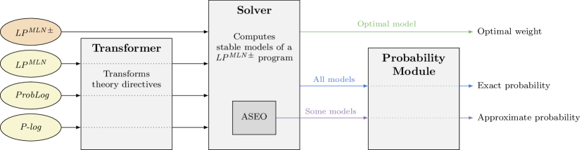
Figure 1: System architecture of plingo. Inputs are yellow for the different frontends provided. Modules of the system are gray boxes. The green flow corresponds to MAP inference, the blue to Exact Marginal Inference, and the purple to Approximate Marginal Inference.

Plingo can be used to solve two reasoning tasks: maximum a posteriori (MAP) inference and marginal inference. MAP inference is the task of finding a most probable stable model of a probabilistic logic program. Following the approach of [10], this task is reduced in plingo to finding one optimal stable model of the input program using clingo’s built-in optimization methods. The only changes that have to be made concern handling the strings that may occur as weights of the weak constraints, and switching the sign of such weights, since otherwise clingo would compute the least probable stable models. Regarding marginal inference, it can be either applied in general, or with respect to a query. In the first case, the task is to find all stable models and their probabilities. In the second case, the task is to find the probability of some query atom, that is defined as the sum of the probabilities of the stable models that contain that atom. The implementation for both cases is the same. First, plingo enumerates all optimal stable models of the input program excluding the weak constraints at level $0$. Afterwards, those optimal stable models are passed, together with their cost at level $0$, to the probability module, that calculates the required probabilities.

In addition to this exact method (represented by the blue arrows in Figure 1), plingo implements an approximation method (purple arrows in Figure 1) based on the approach presented in [15]. The idea is to simplify the solving process by computing just a subset of the stable models, and using this smaller set to approximate the actual probabilities. Formally, in the definitions of $W_{\Pi}^{\mathit{pl}}(X)$ and $P_{\Pi}^{\mathit{pl}}(X)$, this implies replacing the set $\mathit{OSM}^{\mathit{pl}}(\Pi)$ by one of its subsets. In the implementation, the modularity of this change is reflected by the fact that the probability module is agnostic to whether the stable models that it receives as input are all or just some subset of them. For marginal inference in general, this smaller subset consists of $k$ stable models with the highest possible probability, given some positive integer $k$ that is part of the input. To compute this subset, the solver module of plingo uses a new implementation for the task of answer set enumeration in the order of optimality (ASEO) presented in [15]. Given some positive integer $k$, the implementation first computes the stable models of the smallest cost, then, among the remaining stable models, computes the ones of the smallest cost, and so on until $k$ stable models (if they exist) have been computed. For marginal inference with respect to a query, the smaller subset consists of $k$ stable models containing the query of the highest possible probability, and another $k$ stable models without the query of the highest possible probability. In this case, the algorithm for ASEO is set to compute $2k$ stable models. But once it has computed $k$ stable models that contain the query, or $k$ stable models that do not contain the query, whichever happens first, it adds a constraint enforcing that the remaining stable models fall into the opposite case.

6 Experiments

In this section, we experimentally evaluate plingo and compare it to native implementations of $\mathit{LP}^{\mathit{MLN}}$, ProbLog and P-log. For $\mathit{LP}^{\mathit{MLN}}$, we evaluate the system lpmln2asp [10], that is the basis for our implementation of plingo. For ProbLog, we consider the problog system version 2.1 [8], that implements various methods for probabilistic reasoning. In the experiments, we use one of those methods, that is designed specifically to answer probabilistic queries. It converts the input program to a weighted Boolean formula and then applies a knowledge compilation method for weighted model counting. For P-log, we evaluate two implementations, that we call plog-naive and plog-dco [2]. While the former works like plingo and lpmln2asp by enumerating stable models, the latter implements a different algorithm that builds a computation tree specific to the input query. All benchmarks were run on an Intel Xeon E5-2650v4 under Debian GNU/Linux 10, with 24 GB of memory and a timeout of 1200 seconds per instance.

We have performed three experiments. In the first one, our goal is to evaluate the performance of the exact and the approximation methods of plingo  and compare it to the performance of all the other systems on the same domain. In particular, we want to analyze how much faster is the approximation method than the exact one, and how accurate are the probabilities that it returns. In the second experiment, our goal is to compare plingo with the implementations of P-log on domains that are specific to this language. Finally, the goal of the third experiment is to compare plingo and lpmln2asp on the task of MAP inference. In this case, both implementations are very similar and boil down to a single call to clingo. We would like to evaluate if in this situation there is any difference in performance between both systems.

In the first experiment, we compare all systems on the task of marginal inference with respect to a query in a probabilistic Grid domain from [19], that appeared in a slightly different form in [8]. We have chosen this domain because it can be easily and similarly represented in all these probabilistic languages, which is required if we want to compare all systems at the same time. In this domain, there is a grid of size $m\times n$, where each node $(i,j)$ passes information to the nodes $(i+1,j)$ and $(i,j+1)$ if $(i,j)$ is not faulty, and each node in the grid can be faulty with probability $0.1$. The task poses the following question: what is the probability that node $(m,n)$ receives information from node $(1,1)$? To answer this, we run exact marginal inference with all systems, and approximate marginal inference with plingo for different values of $k$: $10^{1}$, $10^{2}$, …, and $10^{6}$. The results are shown in Figure 2. On the left side, there is a cactus plot representing how many instances where solved within a given runtime. The dashed lines represent the runtimes of the approximate marginal inference of plingo for $k=10^{5}$ and $k=10^{6}$. Among the exact implementations, the system problog is the clear winner. In this case, its specific algorithm for answering queries is much faster than the other exact systems that either have to enumerate all stable models or, in the case of plog-dco, may have to explore its whole solution tree. The runtimes among the rest of the exact systems are comparable, but plingo is a bit faster than the others. For the approximation method, on the right side of Figure 2, for every value of $k$ and every instance, there is a dot whose coordinates represent the probability calculated by the approximation method and the true probability (calculated by problog). This is complemented by Table 1, that shows the average absolute error and the maximal absolute error for each value of $k$ in $\%$, where the absolute error for some instance and some $k$ in $\%$ is defined as the absolute value of the difference between the calculated probability and the true probability for that instance, multiplied by $100$. We can see that, as the value of $k$ increases, the performance of the approximation method deteriorates, while the quality of the approximated probabilities increases. A good compromise is found for $k=10^{5}$, where the runtime is better than problog, and the average error is below $1\%$.

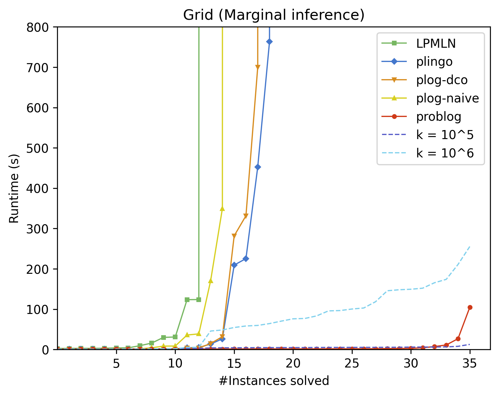
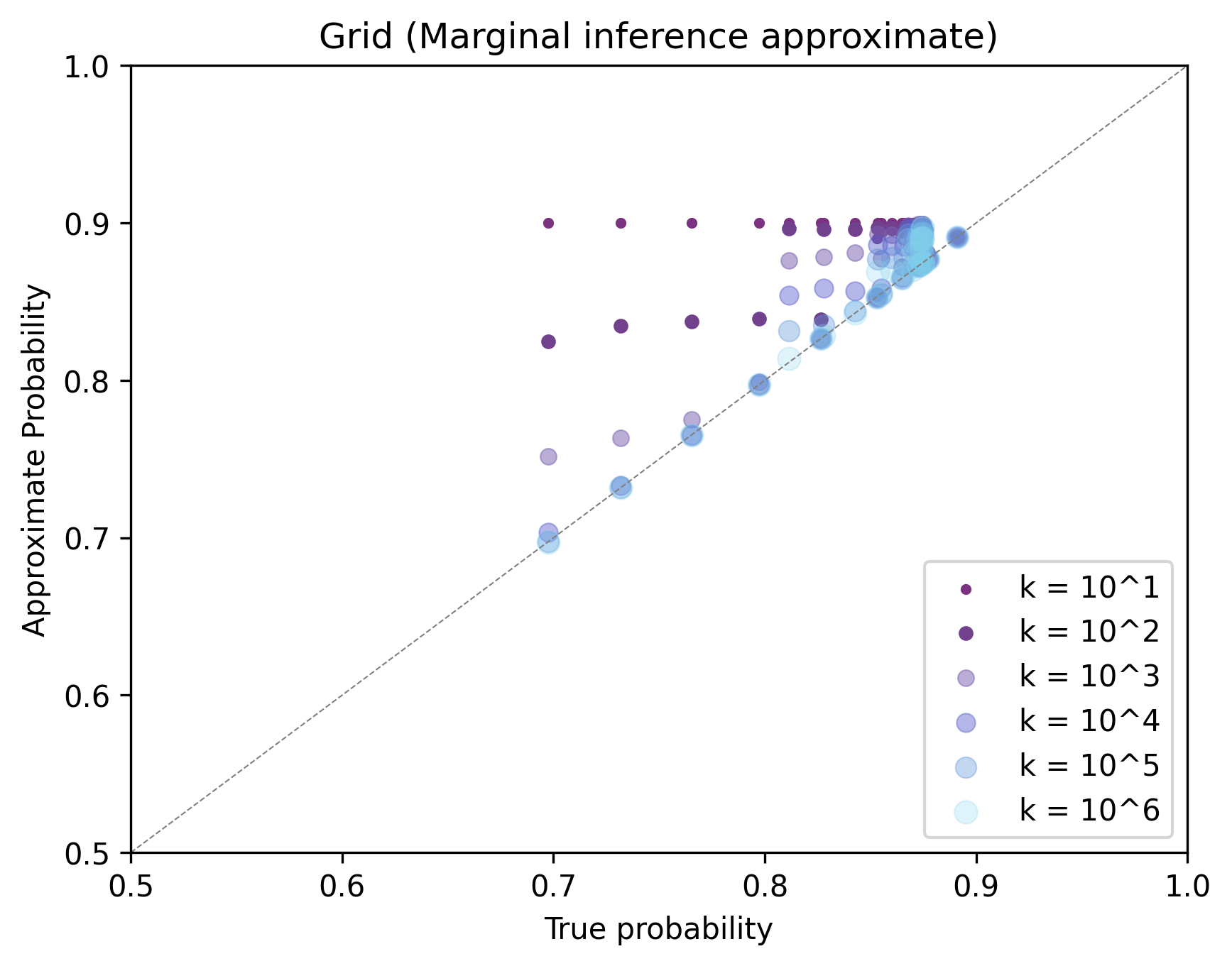
Figure 2: Runtimes of all systems and quality of the approximation method on the Grid domain.

k	$10^{1}$	$10^{2}$	$10^{3}$	$10^{4}$	$10^{5}$	$10^{6}$
Avg. Error	$4.7\pm 4.3$	$3.3\pm 2.7$	$2.1\pm 1.5$	$1.4\pm 1.2$	$0.9\pm 0.9$	$0.6\pm 0.8$
Max. Error	$20.3$	$12.7$	$6.5$	$4.3$	$2.5$	$2.3$

Table 1: Average and maximal error (in $\%$) of the approximation method on the Grid domain for different values of $k$.

In the second experiment, we compare the performance of the exact method of plingo using the P-log frontend with the two native implementations of that language, on tasks of marginal inference with respect to a query in three different domains: NASA, Blocks and Squirrel. The NASA domain ([2]) involves logical and probabilistic reasoning about the faults of a control system. For this domain there are only three instances. All of them are solved by plingo in about a second, while plog-naive takes between $1$ and $5$ seconds, and plog-dco between $40$ and $100$ seconds. The Blocks domain ([19]) starts with a grid and a set of $n$ blocks, and asks what is the probability that two locations are still connected after the $n$ blocks have been randomly placed on the grid. In the experiments we use a single map of $20$ locations and vary $n$ between $1$ and $5$. The results are shown in Figure 3, where we can see a similar pattern as in the NASA domain: plingo and plog-naive solve all instances in just a few seconds, while plog-dco needs much more time for the bigger instances. The Squirrel domain ([2, 3]) is an example of Bayesian learning, where the task is to update the probability of a squirrel finding some food in a patch after failing to find it on $n$ consecutive days. In the experiments we vary the number of days $n$ between $1$ and $27$. The results are shown in figure 3. Now plog-naive is slower and can solve only instances up to $23$ days, while plingo and plog-dco can solve instances up to $27$ days. To interpret the results, recall that the underlying algorithms of plog-naive and plingo are very similar. Hence, we conjecture that the better performance of plingo is due to details of the implementation. On the other hand, plog-dco uses a completely different algorithm. According to the authors ([2]), this algorithm should be faster than plog-naive when the value of the query can be determined from a partial assignment of the atoms of the program. This may be what is happening in the Squirrel domain, where it is on par with plingo, while it does not seem to be the case for the other domains.

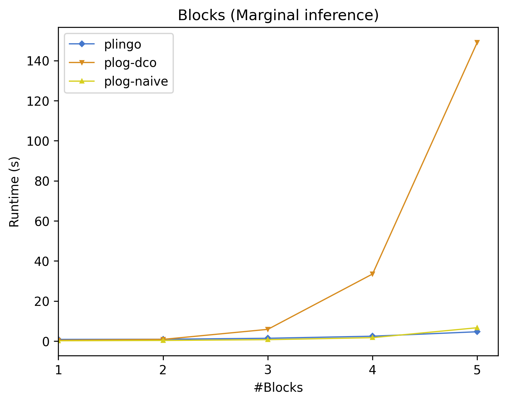
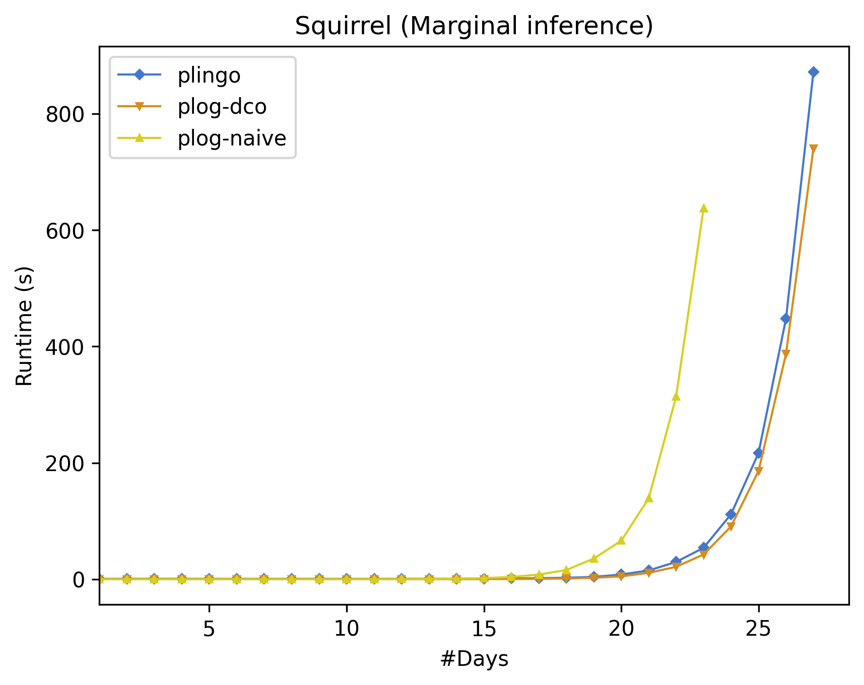
Figure 3: Runtimes of plingo, plog-naive and plog-dco on the P-log domains.

In the third experiment, we compare the performance of the exact method of plingo using the $\mathit{LP}^{\mathit{MLN}}$ frontend with the system lpmln2asp on tasks of MAP inference in two domains: Alzheimer and Smokers. The goal in the Alzheimer domain ([16]) is to determine the probability that two edges are connected in a directed probabilistic graph based on a real-world biological dataset of Alzheimer genes ([18]). The data consists of a directed probabilistic graph with 11530 edges and 5220 nodes. In the experiments we select different subgraphs of this larger graph, varying the number of nodes from $100$ to $2800$. The results are shown in Figure 4, where we observe that for the smaller and bigger instances the performance of plingo and lpmln2asp is quite similar, while in the middle there are some instances that lpmln2asp can solve within the time limit while plingo cannot. The Smokers domain involves probabilistic reasoning about a network of friends. Originally it was presented in [6], but we use a slightly simplified version from [10]. In the experiments we vary the number of friends in the network. In Figure 4, we can observe that for the smaller instances the performance of plingo and lpmln2asp is similar, but for larger instances plingo is faster. Given that the underlying algorithms of plingo and lpmln2asp are similar, we expected them to have a similar performance. Looking at the results, we have no specific explanation for the differences in some instances of the Alzheimer domain, and we conjecture that they are due to the usual variations in solver performance. With respect to the Smokers domain, the worse performance of lpmln2asp seems to be due to the usage of an external parser that increases a lot the preprocessing time for the bigger instances.

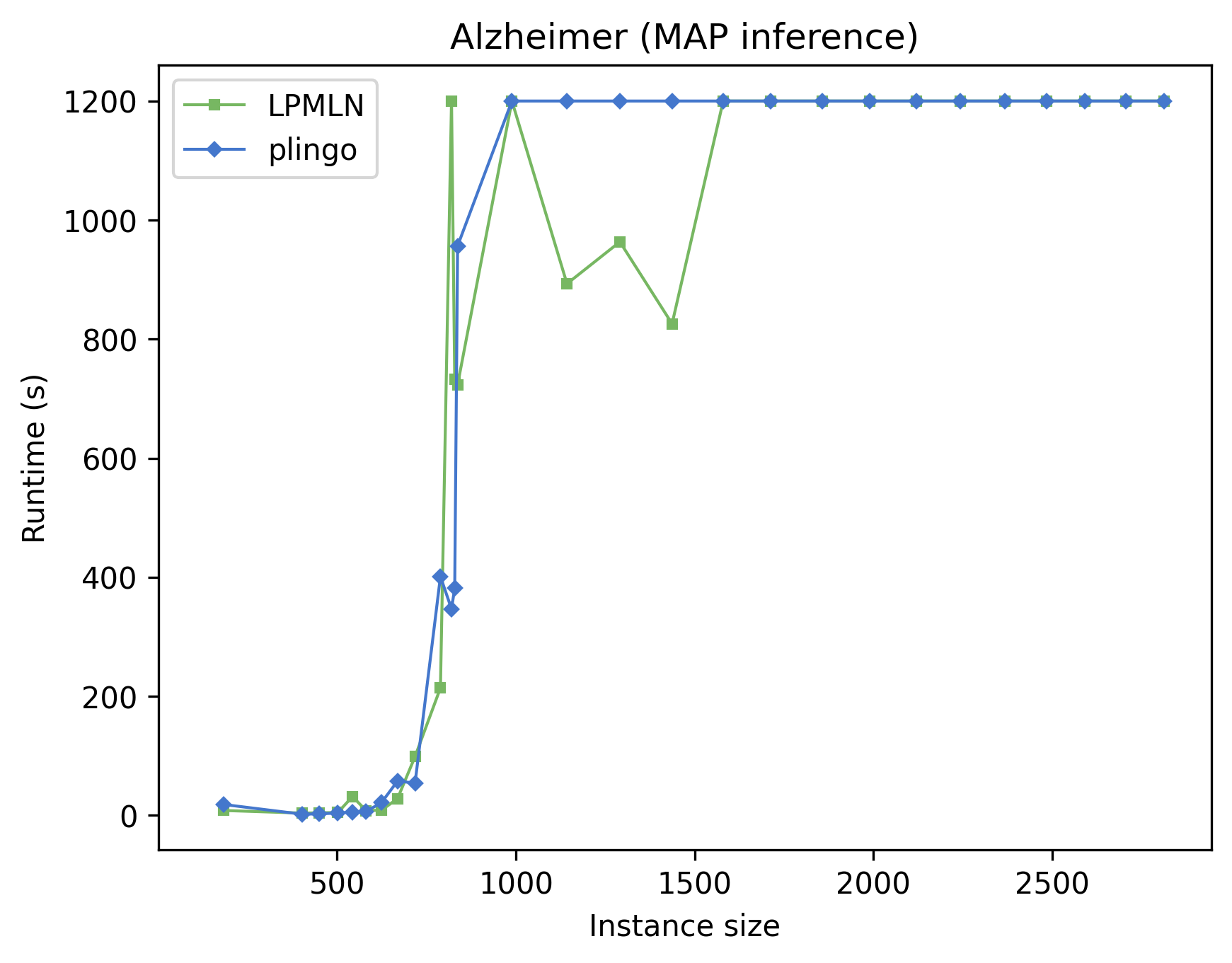
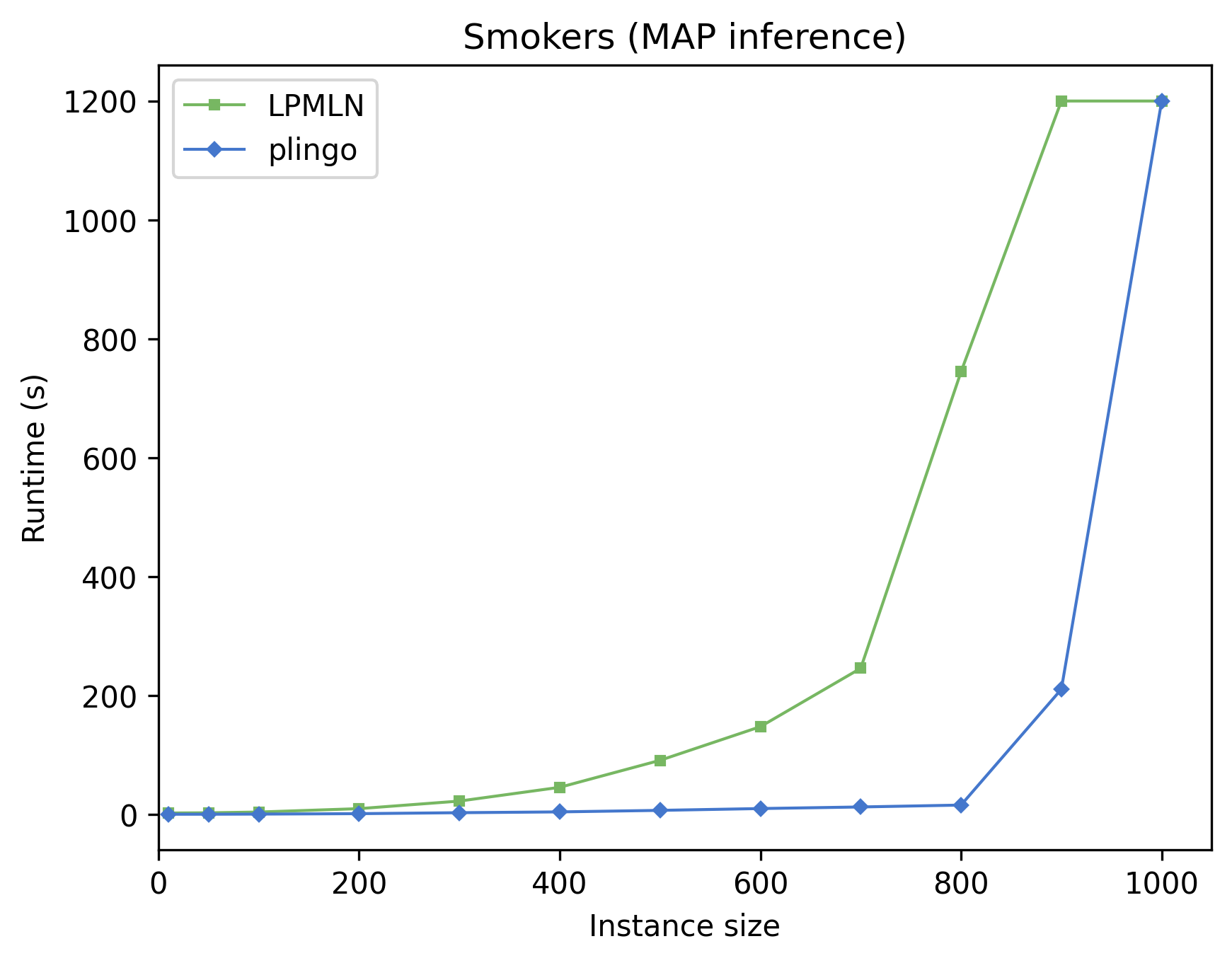
Figure 4: Runtimes of plingo and lpmln2asp on the $\mathit{LP}^{\mathit{MLN}}$ domains.

7 Conclusion

We have presented plingo, an extension of the ASP system clingo with various probabilistic reasoning modes. Although based on $\mathit{LP}^{\mathit{MLN}}$, it also supports P-log and ProbLog. While the basic syntax of plingo is the same as the one of clingo, its semantics relies on re-interpreting the cost of a stable model at priority level $0$ as a measure of its probability. Solving exploits the relation between most probable stable models and optimal stable models [13]; it relies on clingo’s optimization and enumeration modes, as well as an approximation method based on answer set enumeration in the order of optimality [15]. Our empirical evaluation has shown that plingo is at eye height with other ASP-based probabilistic systems, except for problog that relies on well-founded semantics. Notably, the approximation method produced low runtimes and low error rates (below $1\%$). Plingo is freely available at https://github.com/potassco/plingo.

References

- [1] Ahmadi, N., Lee, J., Papotti, P., Saeed, M.: Explainable fact checking with probabilistic answer set programming. In: Liakata, M., Vlachos, A. (eds.) Proceedings of the 2019 Truth and Trust Online Conference (2019)
- [2] Balaii, E.: Investigating and extending P-log. Ph.D. thesis, Texas Tech University (2017)
- [3] Baral, C., Gelfond, M., Rushton, J.: Probabilistic reasoning with answer sets. Theory and Practice of Logic Programming 9(1), 57–144 (2009)
- [4] Buccafurri, F., Leone, N., Rullo, P.: Enhancing disjunctive datalog by constraints. IEEE Transactions on Knowledge and Data Engineering 12(5), 845–860 (2000)
- [5] Calimeri, F., Faber, W., Gebser, M., Ianni, G., Kaminski, R., Krennwallner, T., Leone, N., Ricca, F., Schaub, T.: ASP-Core-2: Input language format. Available at https://www.mat.unical.it/aspcomp2013/ASPStandardization (2012)
- [6] Domingos, P., Kok, S., Lowd, D., Poon, H., Richardson, M., Singla, P.: Probabilistic Inductive Logic Programming - Theory and Applications, Lecture Notes in Computer Science, vol. 4911. Springer-Verlag (2008)
- [7] Ferraris, P.: Answer sets for propositional theories. In: Baral, C., Greco, G., Leone, N., Terracina, G. (eds.) Proceedings of the Eighth International Conference on Logic Programming and Nonmonotonic Reasoning (LPNMR’05). Lecture Notes in Artificial Intelligence, vol. 3662, pp. 119–131. Springer-Verlag (2005)
- [8] Fierens, D., den Broeck, G.V., Renkens, J., Shterionov, D., Gutmann, B., Thon, I., Janssens, G., Raedt, L.D.: Inference and learning in probabilistic logic programs using weighted boolean formulas. Theory and Practice of Logic Programming 15(3), 385–401 (2015)
- [9] Gebser, M., Kaminski, R., Kaufmann, B., Ostrowski, M., Schaub, T., Wanko, P.: Theory solving made easy with clingo 5. In: Carro, M., King, A. (eds.) Technical Communications of the Thirty-second International Conference on Logic Programming (ICLP’16). OpenAccess Series in Informatics (OASIcs), vol. 52, pp. 2:1–2:15. Schloss Dagstuhl–Leibniz-Zentrum fuer Informatik (2016)
- [10] Lee, J., Talsania, S., Wang, Y.: Computing LPMLN using ASP and MLN solvers. Theory and Practice of Logic Programming 17(5-6), 942–960 (2017)
- [11] Lee, J., Wang, Y.: Weighted rules under the stable model semantics. In: C. Baral, J. Delgrande, F.W. (ed.) Proceedings of the Fifteenth International Conference on Principles of Knowledge Representation and Reasoning. pp. 145–154. AAAI/MIT Press (2016)
- [12] Lee, J., Wang, Y.: Weight learning in a probabilistic extension of answer set programs. In: Proceedings of the 16th International Conference on Principles of Knowledge Representation and Reasoning. pp. 22–31 (2018)
- [13] Lee, J., Yang, Z.: LPMLN, weak constraints and P-log. In: Proceedings of the 31st AAAI Conference on Artificial Intelligence. pp. 1170–1177 (2017)
- [14] Lifschitz, V.: Answer set programming and plan generation. Artificial Intelligence 138(1-2), 39–54 (2002)
- [15] Pajunen, J., Janhunen, T.: Solution enumeration by optimality in answer set programming. Theory and Practice of Logic Programming 21(1), 750–767 (2021)
- [16] Raedt, L.D., Kimmig, A., Toivonen, H.: ProbLog: A probabilistic prolog and its applications in link discovery. In: Proceedings of the Twenty-second National Conference on Artificial Intelligence (AAAI’07). pp. 2468–2473. AAAI Press (2007)
- [17] Richardson, M., Domingos, P.: Markov logic networks. Machine Learning 62(1-2), 107–136 (2006)
- [18] Shterionov, D.: Design and Development of Probabilistic Inference Pipelines. Ph.D. thesis, KU Leuven (2015)
- [19] Zhu, W.: Plog: Its algorithms and applications. Ph.D. thesis, Texas Tech University (2012)