A coupled stochastic differential reaction-diffusion system for angiogenesis

Abstract.

A coupled system of nonlinear mixed-type equations modeling early stages of angiogenesis is analyzed in a bounded domain. The system consists of stochastic differential equations describing the movement of the positions of the tip and stalk endothelial cells, due to chemotaxis, durotaxis, and random motion; ordinary differential equations for the volume fractions of the extracellular fluid, basement membrane, and fibrin matrix; and reaction-diffusion equations for the concentrations of several proteins involved in the angiogenesis process. The drift terms of the stochastic differential equations involve the gradients of the volume fractions and the concentrations, and the diffusivities in the reaction-diffusion equations depend nonlocally on the volume fractions, making the system highly nonlinear. The existence of a unique solution to this system is proved by using fixed-point arguments and Hölder regularity theory. Numerical experiments in two space dimensions illustrate the onset of formation of vessels.

1. Introduction

Angiogenesis is the process of expanding existing blood vessel networks by sprouting and branching. Its mathematical modeling is important to understand, for instance, wound healing, inflammation, and tumor growth. In this paper, we analyze a variant of the continuum-scale model suggested in [2] that is used to simulate the early stages of angiogenesis. The model takes into account the dynamics of the tip (leading) endothelial cells by solving stochastic differential equations, the influence of various proteins triggering the cell dynamics by solving reaction-diffusion equations, and the change of some components of the extracellular matrix into extracellular fluid by solving ordinary differential equations. Up to our knowledge, this is the first analysis of the model of [2].

Angiogenesis is mainly triggered by local tissue hypoxia (low oxygen level in the tissue), which activates the production of the signal protein vascular endothelial growth factor (VEGF). Endothelial cells, which form a barrier between vessels and tissues, reached by the VEGF signal initiate the angiogenic program. These cells break out of the vessel wall, degrade the basement membrane (a thin sheet-like structure providing cell and tissue support), proliferate, and invade the surrounding tissue while still connected with the vessel network. The angiogenic program specifies the activated endothelial cells into tip cells (cells at the front of the vascular sprouts) and stalk cells (highly proliferating cells). The tip cells lead the sprout towards the source of VEGF, while the stalk cells proliferate to follow the tip cells supporting sprout elongation; see Figure 1.

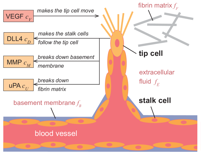
Figure 1. Schematic model of sprout formation in a blood vessel. Tip cells are activated by VEGF and they segrete the proteins DLL4, MMP, and uPA. The vessels are embedded in the fibrin matrix and extracellular fluid and surrounded by the basement membrane.

Following [2], the tip cells segrete the proteins delta-like ligand 4 (DLL4), matrix metalloproteinase (MMP), and urokinase plasminogen activator (uPA). The chemokine DLL4 makes the stalk cells follow the tip cells, MMP breaks down the basement membrane, and uPA degrades the fibrin matrix such that cells can move into. There are many other molecular mechanisms and mediators in the angiogenesis process; see, e.g., [1, 28] for details.

1.1. Model equations

The unknowns are

• the positions $X_{1}^{k}(t)$ of the $k$th tip cell and $X_{2}^{k}(t)$ of the $k$th stalk cell;

• the volume fractions of the basement membrane $f_{B}(x,t)$, the extracellular fluid $f_{E}(x,t)$, and the fibrin matrix $f_{F}(x,t)$;

• the concentrations of the proteins VEGF $c_{V}(x,t)$, DLL4 $c_{D}(x,t)$, MMP $c_{M}(x,t)$, and uPA $c_{U}(x,t)$,

where $t\geq 0$ is the time and $x\in{\mathcal{D}}\subset{\mathbb{R}}^{3}$ the spatial variable. All unknowns depend additionally on the stochastic variable $\omega\in\Omega$, where $\Omega$ is the set of events. We assume that the mixture of basement membrane, extracellular fluid, and fibrine matrix is saturated, i.e., the volume fractions $f_{B}$, $f_{E}$, and $f_{F}$ sum up to one. We introduce the vectors $X=(X_{i}^{k})_{i=1,2,k=1,\ldots,N_{i}}$, $f=(f_{B},f_{E},f_{F})$, and $c=(c_{V},c_{D},c_{M},c_{U})$.

Stochastic differential equations

The tip cells move according to chemotaxis force, driven by the gradient of the VEGF concentration, the durotaxis force, driven by the gradient of the solid fraction $f_{S}:=f_{B}+f_{F}$, and random motion modeling uncertainties. The dynamics of $X_{i}^{k}(t)$ is assumed to be governed by the stochastic differential equations (SDEs)

(1) $${\mathrm{d}}X_{i}^{k}(t)=g_{i}[c,f](X_{i}^{k},t){\mathrm{d}}t+\sigma_{i}(X_{i}^{k}){\mathrm{d}}W_{i}^{k}(t),\quad t>0,\quad X_{i}^{k}(0)=X_{i}^{0},$$

where $i=1,2$, $k=1,\ldots,N_{i}$ for $N_{i}\in{\mathbb{N}}$, $W_{i}^{k}(t)$ are Wiener processes, and the drift terms

(2) $$g_{1}[c,f](X_{1},t) :=\alpha_{0}M_{1}(f_{S}(X_{1}),X_{1})z_{1}+\gamma(f_{S}(X_{1}))\nabla c_{V}(X_{1},t)+\lambda(f_{S}(X_{1}))\nabla f_{S}(X_{1},t),$$

$$g_{2}[c,f](X_{2},t) :=\alpha_{0}M_{2}(f_{S}(X_{2}),X_{2})z_{2}+\gamma(f_{S}(X_{2}))\nabla c_{D}(X_{2},t)+\lambda(f_{S}(X_{2}))\nabla f_{S}(X_{2},t)$$

include a constant $\alpha_{0}>0$, the strain energy $M_{i}$, the direction of movement determined by the strain energy density $z_{i}$, the chemotaxis force $\nabla c_{V}$ in the direction of VEGF (tip cells) and $\nabla c_{D}$ in the direction of DLL4 (stalk cells), and the migration as a result of the durotaxis force $\nabla f_{S}$. In this paper, we allow for general drift terms by imposing suitable Lipschitz continuity conditions; see Assumption (A4) below. In the numerical experiments, we choose the functions $M_{i}$, $\gamma$, and $\lambda$ as in Appendix B.

Ordinary differential equations

The proteins MMP and uPA degrade the basement membrane and fibrin matrix, respectively, while enhancing the extracellular fluid component. Therefore, the volume fractions $f_{B}$, $f_{E}$, and $f_{F}$ are determined by the ordinary differential equations (ODEs)

(3) $$\frac{{\mathrm{d}}f_{B}}{{\mathrm{d}}t} =-s_{B}c_{M}f_{B},\quad t>0,\quad f_{B}(0)=f_{B}^{0},$$

$$\frac{{\mathrm{d}}f_{F}}{{\mathrm{d}}t} =-s_{F}c_{U}f_{F},\quad t>0,\quad f_{F}(0)=f_{F}^{0},$$

$$\frac{{\mathrm{d}}f_{E}}{{\mathrm{d}}t} =s_{B}c_{M}f_{B}+s_{F}c_{U}f_{F},\quad t>0,\quad f_{E}(0)=1-f_{B}^{0}-f_{F}^{0},$$

where $s_{B}$, $s_{F}>0$ are some rate constants. Note that the last differential equation is redundant because of the volume-filling condition $f_{B}+f_{E}+f_{F}=1$. Clearly, equations (3) can be solved explicitly, giving for $(x,t)\in{\mathcal{D}}\times(0,T)$ and pathwise in $\Omega$ (we omit the argument $\omega$),

(4) $$f_{B}(x,t) =f_{B}^{0}(x)\exp\bigg{(}-s_{B}\int_{0}^{t}c_{M}(x,s){\mathrm{d}}s\bigg{)},$$

$$f_{F}(x,t) =f_{F}^{0}(x)\exp\bigg{(}-s_{F}\int_{0}^{t}c_{U}(x,s){\mathrm{d}}s\bigg{)}.$$

Reaction-diffusion equations

The mass concentrations are modeled by reaction-diffusion equations, describing the consumption and production of the proteins:

(5) $$\partial_{t}c_{V}-\operatorname{div}(D_{V}(f)\nabla c_{V})+\alpha_{V}(x,t)c_{V}=0\quad\mbox{in }{\mathcal{D}},\ t>0,$$

$$\partial_{t}c_{D}-\operatorname{div}(D_{D}(f)\nabla c_{D})+\beta_{D}(x,t)c_{D}=\alpha_{D}(x,t)c_{V},$$

$$\partial_{t}c_{M}-\operatorname{div}(D_{M}(f)\nabla c_{M})+s_{M}f_{B}c_{M}=\alpha_{M}(x,t)c_{V},$$

$$\partial_{t}c_{U}-\operatorname{div}(D_{U}(f)\nabla c_{U})+s_{U}f_{F}c_{U}=\alpha_{U}(x,t)c_{V},$$

with initial and no-flux boundary conditions

(6) $$c_{j}(0)=c_{j}^{0}\quad\mbox{in }{\mathcal{D}},\quad\nabla c_{j}\cdot\nu=0\quad\mbox{on }\partial{\mathcal{D}},\ j=V,D,M,U,$$

where the rate terms are given by $\alpha_{V}=s_{V}\widetilde{\alpha}_{V}$, $\alpha_{j}=r_{j}\widetilde{\alpha}_{j}$ for $j=D,M,U$, $\beta_{D}=s_{D}\widetilde{\beta}_{D}$, and

(7) $$\widetilde{\alpha}_{j}(x,t)=\sum_{k=1}^{N_{1}}V_{j}^{k}(X_{1}^{k}(t)-x),\quad\widetilde{\beta}_{D}(x,t)=\sum_{k=1}^{N_{2}}V_{D}^{k}(X_{2}^{k}(t)-x),$$

for $j=V,D,M,U$ and $V_{j}^{k}:\Omega\times{\mathbb{R}}^{3}\to{\mathbb{R}}$ are nonnegative smooth potentials approximating the delta distribution. The parameters $r_{j}$ and $s_{j}$ are positive. In [2], the rate terms are given by delta distributions instead of smooth potentials. We assume smooth potentials because of regularity issues, but they can be given by delta-like functions as long as they are smooth. Indeed, we need $C^{1+\delta}(\overline{\mathcal{D}})$ solutions $c_{j}$ to solve the SDEs (1), and this regularity is not possible when the source terms of (5) include delta distributions. As the number of the proteins is typically much larger than the number of tip cells, the stochastic fluctuations in the concentrations are expected to be much smaller than those associated with the tip cells, which justifies the macroscopic approach using reaction-diffusion equations for the concentrations.

In equation (5) for $c_{V}$, the term $\alpha_{V}c_{V}$ models the consumption of VEGF along the trajectory of the tip cells. The protein DLL4 is regenerated from conversion of VEGF, modeled by $\alpha_{D}c_{V}$ along the trajectories of the tip cells, and consumed by the stalk cells, modeled by $\beta_{D}c_{D}$ along the trajectories of the stalk cells. In equation (5) for $c_{M}$, the term $s_{M}f_{B}c_{M}$ describes the decay of the MMP concentration with rate $s_{B}>0$ as a result of the breakdown of the basement membrane, and $\alpha_{M}c_{V}$ models the production of MMP due to conversion from VEGF. Similary, $s_{U}f_{F}c_{U}$ describes the decay of the uPA concentration, which breaks down the fibrin matrix, and the protein uPA is regenerated, leading to the term $\alpha_{U}c_{V}$.

The diffusivities are given by the mixing rule

$$D_{j}(f)=D_{j}^{B}f_{B}+D_{j}^{E}f_{E}+D_{j}^{F}f_{F},\quad j=V,D,M,U,$$

where $D_{j}^{i}>0$ for $i=B,E,F$. Then

(8) $$0<\min\{D_{j}^{B},D_{j}^{E},D_{j}^{F}\}\leq D_{j}(f)\leq\max\{D_{j}^{B},D_{j}^{E},D_{j}^{F}\},$$

and equations (5) are uniformly parabolic. Note, however, that equations (5) are nonlocal and quasilinear, since the diffusivities are determined by the time integrals of $c_{M}$ or $c_{U}$; see (4).

Various biological phenomena are not modeled by our equations. For instance, we do not include the initiation of sprouting from preexisting parental vessels, the branching from a tip cell, and anastomosis (interconnection between blood vessels). Moreover, in contrast to [2], we do not allow for the transition between the phenotypes “tip cell” and “stalk cell” to simplify the presentation. On the other hand, we may include further angiogenesis-related proteins, if the associated reaction-diffusion equations are of the structure (5).

1.2. State of the art

There are several approaches in the literature to model angiogenesis, mostly in the context of tumor growth. Cellular automata models divide the computational domain into a discrete set of lattice points, and endothelial cells move in a discrete way. Such models are quite flexible, and intra-cellular adherence can be easily implemented, but their numerical solution is computationally expensive when the numbers of cells or molecules are large [12]. In semicontinuous models, the cells are treated as discrete entities, but their movement is not restricted to any lattice points [4]. Continuum-scale models consider cells as averaged quantities, leading to cell densities whose dynamics is described by partial differential equations; see, e.g., [3] for wound healing and [10] for angiogenesis. Chemotaxis can be modeled in this approach by Keller–Segel-type equations, which admit global weak solutions in two space dimensions without blowup [9]. A hybrid approach was investigated in [5], where the blood vessel network is implemented on a lattice, tip cells are moving in a lattice-free way, and other cells are modeled macroscopically as densities. A continuum-scale approach was chosen in [2], which is the basis of the present paper. The novelty of [2] is the distinction of tip and stalk cells and the inclusion of proteins secregated by the tip cells.

In other models, stochastic effects have been included. In [26], the movement of the tip cells is modeled by a SDE, with a deterministic part describing chemotaxis, and a stochastic part modeling random motion. The mean-field limit in a stochastic many-particle system, leading to reaction-diffusion equations, was performed in [6, 25]. We also refer to the reviews [8, 24] on further modeling approaches of angiogenesis.

Numerical simulations of a coupled SDE-PDE model for the movement of the tip cells and the dynamics of the tumor angiogenesis factor, fibronectin (a protein of the extracellular matrix), and matrix degrading enzymes were presented in [7]. Other SDE-PDE models in the literature are concerned with the proton dynamics in a tumor [17], acid-mediated tumor invasion [13], and viscoelastic fluids [14]. However, only the works [13, 17] treat a genuine coupling between SDEs and PDEs. While the model in [13] also includes a cross-diffusion term in the equation for the cancer cells, we have simpler reaction-diffusion equations but with nonlocal diffusivities. Up to our knowledge, the mathematical analysis of system (1), (3)–(6) is new.

1.3. Assumptions and main result

Let $(\Omega,{\mathcal{F}},({\mathcal{F}}_{t})_{t\geq 0},\mathbb{P})$ be a stochastic basis with a complete and right-continuous filtration, and let $(W_{i}^{k}(t))_{t\geq 0}$ for $i=1,2$, $k=1,\ldots,N_{i}$ be independent standard Wiener processes on ${\mathbb{R}}^{d}$ ($d\in{\mathbb{N}}$) relative to $({\mathcal{F}}_{t})_{t\geq 0}$. We write $L^{p}(\Omega,{\mathcal{F}};B)$ for the set of all ${\mathcal{F}}$-measurable random variables with values in a Banach space $B$, for which the $L^{p}$ norm is finite. Furthermore, let ${\mathcal{D}}\subset{\mathbb{R}}^{3}$ be a bounded domain with boundary $\partial{\mathcal{D}}\in C^{3}$ (needed to obtain parabolic regularity; see Theorem 22). We set $Q_{T}={\mathcal{D}}\times(0,T)$.

We write $C^{k+\delta}(\overline{\mathcal{D}})$ with $k\in{\mathbb{N}}_{0}$, $\delta\in(0,1)$ for the space of $C^{k}$ functions $u$ such that the $k$th derivative $\mathrm{D}^{k}u$ is Hölder continuous of index $\delta$. The space of Lipschitz continuous functions on $\overline{\mathcal{D}}$ is denoted by $C^{0,1}(\overline{\mathcal{D}})$. For notational convenience, we do not distinguigh between the spaces $C^{k+\delta}(\overline{\mathcal{D}};{\mathbb{R}}^{n})$ and $C^{k+\delta}(\overline{\mathcal{D}})$. Furthermore, we usually drop the dependence on the variable $\omega\in\Omega$ in the ODEs and PDEs, which hold pathwise $\mathbb{P}$-a.s. Accordingly, we write $c$ instead of $c(\omega,\cdot,\cdot)$ and $c(t)$ instead of $c(\omega,\cdot,t)$. Finally, we write “a.s.” instead of “$\mathbb{P}$-a.s.”.

We impose the following assumptions:

• Initial data: $X^{0}_{i}\in L^{4}(\Omega,{\mathcal{F}}_{0})$ satisfies $X_{i}^{0}\in{\mathcal{D}}$ a.s. ($i=1,2$), $c^{0}\in L^{\infty}(\Omega,{\mathcal{F}}_{0};$ $C^{2+\delta_{0}}(\overline{\mathcal{D}}))$, $f^{0}\in L^{\infty}(\Omega,{\mathcal{F}}_{0};C^{1+\delta_{0}}(\overline{\mathcal{D}}))$ for some $0<\delta_{0}<1$; $c_{j}^{0}\geq 0$ ($j=V,D,M,U$), $f_{i}^{0}\geq 0$ ($i=B,E,F$), and $f_{B}^{0}+f_{E}^{0}+f_{F}^{0}=1$ in ${\mathcal{D}}$ a.s.; $\nabla c_{j}^{0}\cdot\nu=0$ on $\partial{\mathcal{D}}$ a.s.

• Diffusion: $\sigma_{i}:\Omega\times{\mathcal{D}}\times[0,T]\to{\mathbb{R}}^{3\times d}$ ($i=1,2$) is Lipschitz continuous in $x$, has at most linear growth in $x$, is progressively measurable, and satisfies $\sigma_{i}=0$ on $\partial{\mathcal{D}}$ a.s.

• Drift: $g_{i}[c,f]:\Omega\times{\mathcal{D}}\times[0,T]\to{\mathbb{R}}^{3}$ ($i=1,2$) for $f,c\in C^{0}(\overline{\mathcal{D}}\times[0,T])$ is progressively measurable if $(c,f)$ are, and $g_{i}[c,f](x,t)=0$ for $x\in\partial{\mathcal{D}}$, $t\in[0,T]$.

• Lipschitz continuity for $g_{i}$: For $c,c^{\prime},f,f^{\prime}\in C^{1}(\overline{\mathcal{D}}\times[0,T])$, there exists $L_{1}>0$ such that for $(x,t)\in\overline{\mathcal{D}}\times[0,T]$ and $i=1,2$,

  $$\big{|}g_{i}[c,f](x,t)-g_{i}[c^{\prime},f^{\prime}](x,t)\big{|} \leq L_{1}\big{(}1+\|c\|_{L^{\infty}(0,t;C^{1}(\overline{\mathcal{D}}))}+\|f\|_{L^{\infty}(0,t;C^{1}(\overline{\mathcal{D}}))}\big{)}$$

  $$\phantom{xx}{}\times\big{(}\|c(t)-c^{\prime}(t)\|_{C^{1}(\overline{\mathcal{D}})}+\|f(t)-f(t^{\prime})\|_{C^{1}(\overline{\mathcal{D}})}\big{)}.$$

  Furthermore, for $c,f\in L^{\infty}(0,T;W^{2,\infty}({\mathcal{D}}))$, there exists $L_{2}>0$ such that for $(x,t),(x^{\prime},t)\in\overline{\mathcal{D}}\times[0,T]$ and $i=1,2$,

  $$\big{|}g_{i}[c,f](x,t)-g_{i}[c,f](x^{\prime},t)\big{|} \leq L_{2}\big{(}1+\|c\|_{L^{\infty}(0,T;W^{2,\infty}({\mathcal{D}}))}+\|f\|_{L^{\infty}(0,T;W^{2,\infty}({\mathcal{D}}))}\big{)}$$

  $$\phantom{xx}{}\times|x-x^{\prime}|.$$

• Potentials: $V_{j}^{k}\in C^{0,1}({\mathbb{R}}^{3})$ for $j=V,D,M,U$, $k=1,\ldots,N_{i}$ are nonnegative functions.

Let us discuss these assumptions. Since we need $C^{1+\delta}$ solutions $(c,f)$ to obtain Hölder continuous coefficients of the SDEs (which ensures their solvability), we need some regularity conditions on the initial data in Assumption (A1). Accordingly, $\nabla c_{j}^{0}\cdot\nu=0$ on $\partial{\mathcal{D}}$ is a compatibility condition needed for such a regularity result. In Assumption (A1), we impose the volume-filling condition initially, $f_{B}^{0}+f_{E}^{0}+f_{F}^{0}=1$ in ${\mathcal{D}}$. Equations (3) then show that this condition is satisfied for all time. The conditions $\sigma_{i}=0$ and $g_{i}[c,f]=0$ on $\partial{\mathcal{D}}$ in Assumptions (A2) and (A3), respectively, guarantee that the tip and stalk cells do not leave the domain ${\mathcal{D}}$. The conditions on $\sigma_{i}$ in Assumption (A2) and the Lipschitz continuity of $g_{i}[c,f]$ in Assumption (A4) are standard hypotheses to apply existence results for (1). Note that $g_{i}[c,f]$ in example (2) satisfies Assumption (A4). Finally, Assumption (A5) is a simplification to ensure the parabolic regularity results needed, in turn, for the solvability of (1).

Theorem 1 (Global existence).

Let Assumptions (A1)–(A5) hold. Then there exists a unique solution $(X,c,f)$ to (1), (3)–(7) such that

• $X=(X_{i}^{k})_{i=1,2,k=1,\ldots,N_{i}}$ is a strong solution to (1);

• $f=(f_{B},f_{E},f_{F})$ solves (3) pathwise a.s. in the sense of (4), where $f_{i}\in C^{0}([0,T];$ $L^{2}({\mathcal{D}}))\cap L^{\infty}(Q_{T})$;

• $c=(c_{V},c_{D},c_{M},c_{U})$ is a classical solution to (5)–(6) pathwise a.s.

A strong solution $X$ to (1) means, according to [21, Theorem 3.1.1], that $(X_{i}^{k}(t))_{t\geq 0}$ is an a.s. continuous $({\mathcal{F}}_{t})$-adapted process such that for all $t\in[0,T]$,

(9) $$X_{i}^{k}(t)=X_{i}^{0}+\int_{0}^{t}g_{i}[c,f](X_{i}^{k}(s),s){\mathrm{d}}s+\int_{0}^{t}\sigma_{i}(X_{i}^{k}(s)){\mathrm{d}}W_{i}^{k}(s)\quad a.s.$$

1.4. Strategy of the proof

The proof of Theorem 1 is based on a variant of Banach’s fixed-point theorem [19, Theorem 2.4] yielding global solutions. Let $\widetilde{X}$ be a stochastic process with a.s. Hölder continuous paths and values in ${\mathcal{D}}$ a.s. More precisely, $\widetilde{X}_{i}^{k}\in Y_{R}(0,T;{\mathcal{D}})$, where $Y_{R}(0,T;{\mathcal{D}})\subset C^{1/2}([0,T];L^{4}(\Omega))$ is defined in (21) below. Then $\alpha_{j}$ and $\beta_{j}$ are Hölder continuous in $\overline{\mathcal{D}}\times[0,T]$ a.s. as a function of $\widetilde{X}$.

As the first step, we prove the solvability of the ODEs (3) with $c_{j}$ only lying in the space $L^{\infty}(0,T;L^{2}({\mathcal{D}}))$. This is achieved by an approximation argument, assuming a sequence $c_{j}^{(k)}\in L^{\infty}(Q_{T})$ and then passing to the limit. This is possible since the solutions $f_{i}$, represented in (4), are bounded.

Second, we show that there exists a weak solution $c$, which is defined pathwise for $\omega\in\Omega$, to the reaction-diffusion equations (5) by using a Galerkin method and the fixed-point theorem of Schauder for fixed $\alpha_{j}$ and $\beta_{j}$. The regularity of $c$ can be improved step by step. Moser’s iteration method shows that the weak solution is in fact bounded, and a general regularity result for evolution equations yields $\partial_{t}c\in L^{2}(Q_{T})$. Then, interpreting equations (5) as elliptic equations with right-hand side $\partial_{t}c\in L^{2}(Q_{T})$, we conclude the Hölder continuity of $c(t)$ for any fixed $t\in(0,T)$. Thus, the diffusivities are Hölder continuous, and we infer $C^{1+\delta}(\overline{\mathcal{D}})$ and $W^{2,\infty}({\mathcal{D}})$ solutions $c$. We conclude classical solvability from the regularity results of Ladyženskaya et al. [18].

In the third step, we solve the SDEs (1). The functions $(c,f)$ have Hölder continuous gradients, and we show that $(c,f)$ and $(\nabla c,\nabla f)$ are progressively measurable. Therefore, together with Assumption (A4), the conditions of the existence theorem of [21, Theorem 3.1.1] are satisfied, and we obtain a solution $X$ to (1) in the sense (9).

Fourth, defining a suitable complete metric space $Y_{R}(0,T;{\mathcal{D}})$, endowed with the $C^{0}([0,T];$ $L^{4}({\mathcal{D}}))$ norm, this defines the fixed-point operator $\Phi:\widetilde{X}\mapsto X$ on $Y_{R}(0,T;{\mathcal{D}})$. The fixed-point operator can be written as the contatenation

$$\Phi:\widetilde{X}\mapsto(\alpha,\beta_{D})\mapsto(c,f)\mapsto X,$$

where $\alpha=(\alpha_{V},\alpha_{D},\alpha_{M},\alpha_{U})$. It remains to show that $\Phi$ is a self-mapping and a contraction, which is possible for a sufficiently large $R>0$. In fact, we show that for any $n\in{\mathbb{N}}$,

$$\sup_{0<s<t}\big{(}\mathbb{E}|\Phi^{n}(X(t))-\Phi^{n}(X^{\prime}(t))|^{4}\big{)}^{1/4}\leq c_{n}\sup_{0<s<t}\big{(}\mathbb{E}|X(t)-X^{\prime}(t)|^{4}\big{)}^{1/4}$$

for all $X$, $X^{\prime}\in Y_{R}(0,T;{\mathcal{D}})$, where $c_{n}\to 0$ as $n\to\infty$. It follows from the variant of Banach’s fixed-point theorem in [19, Theorem 2.4] that $\Phi$ has a unique fixed point, which gives a unique solution $(X,c,f)$ to (1), (3)–(7).

The paper is organized as follows. The solvability of the ODEs (3) for $L^{2}({\mathcal{D}})$ coefficients and a stability estimate are shown in Section 2. In Section 3, the existence of a unique classical solution to the reaction-diffusion equations (5)–(6) and some stability results are proved. The progressive measurability of the solutions to (3) and (5) as well as the solvability of the SDEs (1) is verified in Section 4. Based on these results, Theorem 1 is proved in Section 5. Some numerical experiments are illustrated in Section 6, showing stalk cells following the tip cells and forming a premature sprout. Appendix A summarizes some regularity results for elliptic and parabolic equations used in this work, and Appendix B collects the numerical values of the various parameters used in the numerical experiments.

2. Solution of ODEs in Bochner spaces

We prove a result for ODEs in some Bochner space, which is needed for the solution of (3) when the concentrations $c_{j}$ are only $L^{2}({\mathcal{D}})$ functions.

Lemma 2.

Let $u\in L^{\infty}(0,T;L^{2}({\mathcal{D}}))$ and $g^{0}\in L^{\infty}({\mathcal{D}})$ be nonnegative functions. Then

(10) $$\frac{{\mathrm{d}}g}{{\mathrm{d}}t}=-ug,\quad t>0,\quad g(0)=g^{0}\quad\mbox{a.e. in }{\mathcal{D}},$$

has a unique solution $g\in C^{0}([0,T];L^{2}({\mathcal{D}}))\cap L^{\infty}(Q_{T})$ satisfying $0\leq g\leq\|g^{0}\|_{L^{\infty}({\mathcal{D}})}$ a.e. in $Q_{T}$.

Proof.

Set $[u]_{k}:=\max\{k,u\}=u(t)-(u(t)-k)^{+}$ for $k\geq 0$, where $z^{+}=\max\{0,z\}$. We claim that $[u]_{k}\in L^{\infty}(Q_{T})$ has the properties $[u(t)]_{k}\to u(t)$ strongly in $L^{2}({\mathcal{D}})$ as $k\to\infty$ for a.e. $t\in[0,T]$ and

(11) $$\|[u(t)]_{k}-[u(t)]_{j}\|_{L^{2}({\mathcal{D}})}\leq\|[u(t)]_{j}-u(t)\|_{L^{2}({\mathcal{D}})}\leq C\quad\mbox{a.e. in }[0,T]$$

for $0\leq j\leq k$, where $C>0$ does not depend on $k$ or $j$. Indeed, the first inequality follows from

$$\|[u (t)]_{k}-[u(t)]_{j}\|_{L^{2}({\mathcal{D}})}^{2}=\int_{\mathcal{D}}\big{(}(u(t)-k)^{+}-(u(t)-j)^{+}\big{)}^{2}{\mathrm{d}}x$$

$$=\int_{\{u(t)\geq k\}}\big{(}(u(t)-k)^{+}-(u(t)-j)^{+}\big{)}^{2}{\mathrm{d}}x+\int_{\{j\leq u(t)\leq k\}}[(u(t)-j)^{+}]^{2}{\mathrm{d}}x$$

$$=\int_{\{u(t)\geq k\}}(k-j)^{2}{\mathrm{d}}x+\int_{\{j\leq u(t)\leq k\}}(u(t)-j)^{2}{\mathrm{d}}x$$

$$\leq\int_{\{u(t)\geq k\}}(u(t)-j)^{2}{\mathrm{d}}x+\int_{\{j\leq u(t)\leq k\}}(u(t)-j)^{2}{\mathrm{d}}x$$

$$=\int_{\mathcal{D}}[(u(t)-j)^{+}]^{2}{\mathrm{d}}x=\|[u(t)]_{j}-u(t)\|_{L^{2}({\mathcal{D}})}^{2}.$$

Furthermore, we have

$$\|[u(t)]_{j}-u(t)\|_{L^{2}({\mathcal{D}})}^{2}=\int_{\mathcal{D}}[(u(t)-j)^{+}]^{2}{\mathrm{d}}x\leq\|u\|^{2}_{L^{\infty}(0,T;L^{2}({\mathcal{D}}))}\leq C.$$

The function $u(t)^{2}$ is an integrable upper bound for $(u(t)-k)^{+}$. Furthermore, $[u(t)]_{k}-u(t)=-(u(t)-k)^{+}$ converges to zero a.e. in ${\mathcal{D}}$ as $k\to\infty$. Therefore, we conclude from dominated convergence that $[u(t)]_{k}-u(t)\to 0$ strongly in $L^{2}({\mathcal{D}})$. This proves the claim.

Next, we consider the differential equation

(12) $$\frac{{\mathrm{d}}g_{k}}{{\mathrm{d}}t}=-[u]_{k}g_{k},\quad t>0,\quad g_{k}(0)=g^{0}\quad\mbox{a.e. in }{\mathcal{D}}.$$

Since $[u]_{k}$ is bounded, there exists a unique solution $g_{k}\in C^{0}([0,T];L^{\infty}({\mathcal{D}}))$, given by

$$g_{k}(t)=g^{0}\exp\bigg{(}-\int_{0}^{t}[u(s)]_{k}{\mathrm{d}}s\bigg{)},\quad 0<t<T.$$

Clearly, we have $0<g_{k}(t)\leq K:=\|g^{0}\|_{L^{\infty}({\mathcal{D}})}$. We want to prove that $(g_{k})$ converges as $k\to\infty$ to a solution of the original equation. It follows that

$$\frac{1}{2} \frac{{\mathrm{d}}}{{\mathrm{d}}t}\|g_{k}-g_{j}\|_{L^{2}({\mathcal{D}})}^{2}=-\int_{\mathcal{D}}([u]_{k}g_{k}-[u]_{j}g_{j})(g_{k}-g_{j}){\mathrm{d}}x$$

$$=-\int_{\mathcal{D}}[u]_{k}(g_{k}-g_{j})^{2}{\mathrm{d}}x-\int_{\mathcal{D}}([u]_{k}-[u]_{j})g_{j}(g_{k}-g_{j}){\mathrm{d}}x$$

$$\leq\frac{K}{2}\|[u]_{k}-[u]_{j}\|_{L^{2}({\mathcal{D}})}^{2}+\frac{K}{2}\|g_{k}-g_{j}\|_{L^{2}({\mathcal{D}})}^{2}.$$

We conclude from Gronwall’s lemma and (11) that

$$\|g_{k}(t)-g_{j}(t)\|_{L^{2}({\mathcal{D}})}^{2} \leq\int_{0}^{t}e^{K(t-s)}\|[u(s)]_{k}-[u(s)]_{j}\|_{L^{2}({\mathcal{D}})}^{2}{\mathrm{d}}s$$

$$\leq e^{Kt}\int_{0}^{t}\|[u(s)]_{j}-u(s)\|_{L^{2}({\mathcal{D}})}^{2}{\mathrm{d}}s.$$

Because of $\|[u(s)]_{j}-u(s)\|_{L^{2}({\mathcal{D}})}^{2}\to 0$ as $j\to\infty$ and the uniform upper bound for $[u(s)]_{j}-u(s)$, the dominated convergence theorem implies that, for any $t\in[0,T]$,

$$\|g_{k}(t)-g_{j}(t)\|_{L^{2}({\mathcal{D}})}^{2}\leq e^{KT}\int_{0}^{T}\|[u(s)]_{j}-u(s)\|_{L^{2}({\mathcal{D}})}^{2}{\mathrm{d}}s\to 0\quad\mbox{as }j,k\to\infty.$$

Thus, $(g_{k}(t))$ is a Cauchy sequence for every $t\in[0,T]$ and we infer that $g_{k}(t)\to g(t)$ in $L^{2}({\mathcal{D}})$. Because of the $L^{\infty}(0,T;L^{2}({\mathcal{D}}))$ bound for $(g_{k})$ and dominated convergence again, $g_{k}\to g$ in $L^{2}(Q_{T})$, where $g\in L^{\infty}(0,T;L^{2}({\mathcal{D}}))$. There exists a subsequence, which is not relabeled, such that $g_{k}(t)\to g(t)$ a.e. in ${\mathcal{D}}$, for any $t\in[0,T]$. We deduce from $g_{k}(t)\leq K$ that $g(t)\leq K$ for all $t\in[0,T]$. This shows that $g\in L^{\infty}(Q_{T})$. Writing (12) as an integral equation and performing the limit $k\to\infty$, the previous convergence results show that $g$ solves (10). ∎

We also need the following stability result, which relates the difference $f_{1}-f_{2}$ of solutions to (3) with the difference $c_{1}-c_{2}$ of solutions to (5).

Lemma 3.

Let $u_{1}$, $u_{2}\in L^{\infty}(0,T;W^{k,\infty}({\mathcal{D}}))$ with $k\in{\mathbb{N}}_{0}$, $g_{1}^{0}$, $g_{2}^{0}\in W^{k,\infty}({\mathcal{D}})$, and let $g_{1}$, $g_{2}\in C^{0}([0,T];W^{k,\infty}({\mathcal{D}}))$ be the unique solutions to

$$\frac{{\mathrm{d}}g_{i}}{{\mathrm{d}}t}=-u_{i}g_{i},\quad 0<t<T,\quad g_{i}(0)=g_{i}^{0}\quad\mbox{a.e. in }{\mathcal{D}},\ i=1,2.$$

Then there exists $C>0$, only depending on $T$, the $L^{\infty}(0,T;W^{k,\infty}({\mathcal{D}}))$ norm of $u_{i}$, and the $W^{k,\infty}({\mathcal{D}})$ norm of $g_{i}^{0}$, such that for $p>1$,

$$\|g_{1}-g_{2}\|_{W^{k,p}({\mathcal{D}})}\leq C\big{(}\|g_{1}^{0}-g_{2}^{0}\|_{W^{k,p}({\mathcal{D}})}+\|u_{1}-u_{2}\|_{L^{1}(0,T;W^{k,p}({\mathcal{D}}))}\big{)}.$$

Proof.

The regularity of $g_{i}$ follows from the explicit formula and the regularity for $g_{i}^{0}$ and $u_{i}$. Furthermore, taking the $W^{k,p}({\mathcal{D}})$ norm of

$$g_{1}(t)-g_{2}(t)=g_{1}^{0}-g_{2}^{0}-\int_{0}^{t}\big{(}u_{1}(g_{1}-g_{2})+(u_{1}-u_{2})g_{2}\big{)}{\mathrm{d}}x,$$

the result follows from the regularity $u_{1}\in L^{\infty}(0,T;W^{k,\infty}({\mathcal{D}}))$ and $g_{2}\in W^{k,\infty}({\mathcal{D}})$. ∎

3. Solution of the reaction-diffusion equations

We show the existence of a weak solution to (5)–(6) for given $\alpha$, $\beta_{D}$ and then prove that this solution is in fact a classical one.

3.1. Existence of weak solutions

The existence of solutions to the reaction-diffusion equations (5) is shown by using the Galerkin method and the fixed-point theorem of Schauder.

Lemma 4 (Existence for (5)).

Let $\alpha_{j}$, $\beta_{D}\in L^{\infty}(Q_{T})$, $\alpha_{j}\geq 0$, $\beta_{D}\geq 0$ for $j=V,D,M,U$, $c^{0}\in L^{2}({\mathcal{D}})$, and $f\in L^{\infty}({\mathcal{D}})$ satisfying $f_{B}+f_{E}+f_{F}=1$ in ${\mathcal{D}}$. Then there exists a weak solution $c=(c_{V},c_{D},c_{M},c_{U})$ to (5)–(6).

Proof.

Let $(e_{\ell})_{\ell\in{\mathbb{N}}}$ be the sequence of eigenfunctions of the Laplace operator with homogeneous Neumann boundary conditions. They form an orthonormal basis of $L^{2}({\mathcal{D}})$ and are orthogonal with respect to the $H^{1}({\mathcal{D}})$ norm. The boundary regularity $\partial{\mathcal{D}}\in C^{3}$ guarantees that $e_{\ell}\in H^{3}({\mathcal{D}})\hookrightarrow C^{1}(\overline{\mathcal{D}})$; see Theorem 18 in the Appendix. Let $E_{N}=\operatorname{span}\{e_{1},\ldots,e_{N}\}$ for $N\in{\mathbb{N}}$. We wish to find a solution $c^{N}\in C^{0}([0,T];E_{N})$ to the finite-dimensional problem

(13) $$(\partial_{t}c_{V}^{N},\phi_{V})_{L^{2}}+(D_{V}(f^{N})\nabla c_{V}^{N},\nabla\phi_{V})_{L^{2}} =-(\alpha_{V}c_{V}^{N},\phi_{V})_{L^{2}},$$

$$(\partial_{t}c_{D}^{N},\phi_{D})_{L^{2}}+(D_{D}(f^{N})\nabla c_{D}^{N},\nabla\phi_{D})_{L^{2}} =(\alpha_{D}c_{V}^{N},\phi_{D})_{L^{2}}-(\beta_{D}c_{D}^{N},\phi_{D})_{L^{2}},$$

$$(\partial_{t}c_{M}^{N},\phi_{M})_{L^{2}}+(D_{M}(f^{N})\nabla c_{M}^{N},\nabla\phi_{M})_{L^{2}} =(\alpha_{M}c_{V}^{N},\phi_{M})_{L^{2}}-s_{M}(f_{B}^{N}c_{M}^{N},\phi_{M})_{L^{2}},$$

$$(\partial_{t}c_{U}^{N},\phi_{U})_{L^{2}}+(D_{U}(f^{N})\nabla c_{U}^{N},\nabla\phi_{U})_{L^{2}} =(\alpha_{U}c_{V}^{N},\phi_{U})_{L^{2}}-s_{U}(f_{F}^{N}c_{U}^{N},\phi_{U})_{L^{2}}$$

for all $\phi=(\phi_{V},\phi_{D},\phi_{M},\phi_{U})\in E_{N}^{4}$, where $(\cdot,\cdot)_{L^{2}}$ denotes the inner product in $L^{2}({\mathcal{D}})$, together with the initial condition $c^{N}(0)=c^{0,N}$. Here, $c^{0,N}\in E_{N}$ satisfies $c^{0,N}\to c^{0}$ in $L^{2}({\mathcal{D}})$ as $N\to\infty$. The function $f^{N}=(f_{B}^{N},f_{F}^{N},f_{E}^{N})$ is the solution to (3) with $c_{j}$ replaced by $(c_{j}^{N})^{+}:=\max\{0,c_{j}^{N}\}$. An integration gives

$$f_{B}^{N}(t)=f^{0}_{B}\exp\bigg{(}-s_{B}\int_{0}^{t}(c_{M}^{N})^{+}(s){\mathrm{d}}s\bigg{)},\quad f_{F}(t)=f^{0}_{F}\exp\bigg{(}-s_{F}\int_{0}^{t}(c_{U}^{N})^{+}(s){\mathrm{d}}s\bigg{)},$$

and $f_{E}^{N}(t):=1-f_{B}^{N}(t)-f_{F}^{N}(t)$ for $0<t<T$.

To solve (13), we consider first a linearized version. Let $\widehat{c}^{N}\in C^{0}([0,T];E_{N})$ be given. Then

(14) $$(\partial_{t}c_{V}^{N},\phi_{V})_{L^{2}}+(D_{V}(\widehat{f}^{N})\nabla c_{V}^{N},\nabla\phi_{V})_{L^{2}} =-(\alpha_{V}c_{V}^{N},\phi_{V})_{L^{2}},$$

$$(\partial_{t}c_{D}^{N},\phi_{D})_{L^{2}}+(D_{D}(\widehat{f}^{N})\nabla c_{D}^{N},\nabla\phi_{D})_{L^{2}} =(\alpha_{D}c_{V}^{N},\phi_{D})_{L^{2}}-(\beta_{D}c_{D}^{N},\phi_{D})_{L^{2}},$$

$$(\partial_{t}c_{M}^{N},\phi_{M})_{L^{2}}+(D_{M}(\widehat{f}^{N})\nabla c_{M}^{N},\nabla\phi_{M})_{L^{2}} =(\alpha_{M}c_{V}^{N},\phi_{M})_{L^{2}}-s_{M}(\widehat{f}_{B}^{N}c_{M}^{N},\phi_{M})_{L^{2}},$$

$$(\partial_{t}c_{U}^{N},\phi_{U})_{L^{2}}+(D_{U}(\widehat{f}^{N})\nabla c_{U}^{N},\nabla\phi_{U})_{L^{2}} =(\alpha_{U}c_{V}^{N},\phi_{U})_{L^{2}}-s_{U}(\widehat{f}_{F}^{N}c_{U}^{N},\phi_{U})_{L^{2}}$$

for any $\phi\in E_{N}^{4}$, with the initial condition $c^{N}(0)=c^{0,N}$,

$$\widehat{f}_{B}^{N}(t)=f^{0}_{B}\exp\bigg{(}-s_{B}\int_{0}^{t}(\widehat{c}_{M}^{N})^{+}(s){\mathrm{d}}s\bigg{)},\quad\widehat{f}_{F}^{N}(t)=f^{0}_{F}\exp\bigg{(}-s_{F}\int_{0}^{t}(\widehat{c}_{U}^{N})^{+}(s){\mathrm{d}}s\bigg{)},$$

and $\widehat{f}_{E}^{N}(t):=1-\widehat{f}_{B}^{N}(t)-\widehat{f}_{F}^{N}(t)$ for $0<t<T$, is a system of linear ordinary differential equations in the variables $d_{j\ell}^{N}$, where $c_{j}^{N}(t)=\sum_{\ell=1}^{N}d_{j\ell}^{N}(t)e_{\ell}$, $j=V,D,M,U$. By standard ODE theory, there exists a unique solution $c^{N}(t)$ for $t\in[0,T]$. Taking $\phi_{j}=c_{j}^{N}$ for $j=V,D,M,U$ as test functions in (14) and using the positive lower and upper bounds (8) of the diffusivities as well as the $L^{\infty}$ bound for $\widehat{f}$, standard computations lead to the estimates

(15) $$\|c^{N}\|_{L^{\infty}(0,T;L^{2}({\mathcal{D}}))}+\|c^{N}\|_{L^{2}(0,T;H^{1}({\mathcal{D}}))}+\|\partial_{t}c^{N}\|_{L^{2}(0,T;H^{1}({\mathcal{D}})^{\prime})} \leq C(T,c^{0}),$$

$$\|c^{N}\|_{L^{\infty}(0,T;H^{1}({\mathcal{D}}))} \leq C(N).$$

In the following, the notation $(E_{N};\|\cdot\|_{Z})$ means that $E_{N}$ is endowed with the norm of the Banach space $Z$, requiring that $E_{N}\subset Z$.

We wish to define a fixed-point operator $\widehat{c}^{N}\mapsto c^{N}$. For this, we introduce the sets

$$Y =\big{\{}u\in L^{\infty}(0,T;(E_{N};\|\cdot\|_{H^{1}({\mathcal{D}})})):\partial_{t}u\in L^{2}(0,T;(E_{N};\|\cdot\|_{H^{1}({\mathcal{D}})})^{\prime})\big{\}},$$

$$Y_{b} =\big{\{}u\in Y:\|u\|_{L^{\infty}(0,T;H^{1}({\mathcal{D}}))}+\|\partial_{t}u\|_{L^{2}(0,T;H^{1}({\mathcal{D}})^{\prime})}\leq C(T,c^{0})+C(N)\big{\}},$$

and $W$ is defined as the closure of $Y_{b}^{4}$ with respect to the $C^{0}([0,T];L^{2}({\mathcal{D}}))$ norm. We claim that the embedding $W\hookrightarrow C^{0}([0,T];(E_{N};L^{2}({\mathcal{D}})))$ is compact. Indeed, $(E_{N};H^{1}({\mathcal{D}}))$ is compactly embedded into $(E_{N};L^{2}({\mathcal{D}}))$. By the Aubin–Lions lemma, $Y$ is compactly embedded into $C^{0}([0,T];(E_{N};L^{2}({\mathcal{D}})))$. Consequently, $W=\overline{Y_{b}}^{4}$ is compactly embedded into $C^{0}([0,T];(E_{N};L^{2}({\mathcal{D}})))$.

This defines the fixed-point operator $S:W\to C^{0}([0,T];(E_{N};L^{2}({\mathcal{D}})))$. Estimates (15) show that $S(W)\subset Y_{b}^{4}\subset W$. Furthermore, we can prove by standard arguments that $S:W\to W$ is continuous. We deduce from Schauder’s fixed-point theorem that there exists a fixed point $c^{N}$ of $S$ satisfying (13).

Now, we perform the limit $N\to\infty$. Estimates (15) allow us to apply the Aubin–Lions lemma, giving the existence of a subsequence (not relabeled) such that, as $N\to\infty$,

$$c^{N}\to c\quad\mbox{strongly in }L^{2}(0,T;L^{2}({\mathcal{D}}))$$

for some $c\in L^{2}(0,T;H^{1}({\mathcal{D}}))\cap H^{1}(0,T;H^{1}({\mathcal{D}})^{\prime})$. Moreover,

$$c^{N}\rightharpoonup c \quad\mbox{weakly in }L^{2}(0,T;H^{1}({\mathcal{D}})),$$

$$\partial_{t}c^{N}\rightharpoonup\partial_{t}c \quad\mbox{weakly in }L^{2}(0,T;H^{1}({\mathcal{D}})^{\prime}).$$

We define

$$f_{B}(t)=f_{B}^{0}\exp\bigg{(}-s_{B}\int_{0}^{t}c_{M}^{+}(s){\mathrm{d}}s\bigg{)},\quad f_{F}(t)=f_{F}^{0}\exp\bigg{(}-s_{F}\int_{0}^{t}c_{U}^{+}(s){\mathrm{d}}s\bigg{)},$$

and $f_{E}(t):=1-f_{B}(t)-f_{F}(t)$ for $0<t<T$. Lemma 3 implies that

$$\|f_{B}^{N}-f_{B}\|_{L^{2}(Q_{T})}\leq C(T)\|c_{M}^{N}-c_{M}\|_{L^{2}(Q_{T})}\to 0\quad\mbox{as }N\to\infty.$$

We infer from the linear dependence of $D_{j}(f)$ on $f$ that $D_{j}(f^{N})-D_{j}(f)\to 0$ strongly in $L^{2}(Q_{T})$ for $j=V,D,M,U$. This shows that $D_{j}(f^{N})\nabla c_{j}^{N}\to D_{j}(f)\nabla c_{j}$ weakly in $L^{1}(Q_{T})$ for $j=V,D,M,U$ and $s_{M}f_{B}^{N}c_{M}^{N}\to s_{M}f_{B}c_{M}$, $s_{U}f_{F}^{N}c_{U}^{N}\to s_{U}f_{F}c_{U}$ strongly in $L^{1}(Q_{T})$. Thus, passing to the limit $N\to\infty$ in equation (13) for $c_{M}^{N}$,

$$\langle\partial_{t}c_{M},\phi\rangle+(D_{M}(f)\nabla c_{M},\nabla\phi)_{L^{2}}=(\alpha_{M}c_{M},\phi)_{L^{2}}-s_{M}(f_{B}c_{M},\phi)_{L^{2}}$$

for all test functions $\phi(x,t)=\sum_{k=1}^{N}t^{k}e_{k}\in C^{1}(\overline{{\mathcal{D}}}\times[0,T])$ and similarly for the other equations in (13). Here, $\langle\cdot,\cdot\rangle$ denotes the dual product between $H^{1}({\mathcal{D}})$ and $H^{1}({\mathcal{D}})^{\prime}$. Since the class of functions $\phi$ of this type is dense in $L^{2}(0,T;H^{1}({\mathcal{D}}))\cap H^{1}(0,T;H^{1}({\mathcal{D}})^{\prime})$ [30, Prop. 23.23iii], we conclude that $(c,f)$ is a weak solution to (3)–(6).

It remains to verify that the limit concentration $c$ is nonnegative componentwise. We use $c_{V}^{-}=\min\{0,c_{V}\}$ as a test function in the weak formulation of equation (5) for $c_{V}$:

$$\frac{1}{2}\frac{{\mathrm{d}}}{{\mathrm{d}}t}\int_{\mathcal{D}}(c_{V}^{-})^{2}{\mathrm{d}}x+\int_{\mathcal{D}}D_{V}(f)|\nabla c_{V}^{-}|^{2}{\mathrm{d}}x=-\int_{\mathcal{D}}\alpha_{V}(c_{V}^{-})^{2}{\mathrm{d}}x\leq 0,$$

which yields $c_{V}^{-}(t)=0$ and $c_{V}(t)\geq 0$ in ${\mathcal{D}}$, $t>0$. Next, we use $c_{D}^{-}$ as a test function in the weak formulation of equation (5) for $c_{D}$:

$$\frac{1}{2}\frac{{\mathrm{d}}}{{\mathrm{d}}t}\int_{\mathcal{D}}(c_{D}^{-})^{2}{\mathrm{d}}x+\int_{\mathcal{D}}D_{D}(f)|\nabla c_{D}^{-}|^{2}{\mathrm{d}}x=-\int_{\mathcal{D}}\beta_{D}(c_{D}^{-})^{2}{\mathrm{d}}x+\int_{\mathcal{D}}\alpha_{D}c_{V}c_{D}^{-}{\mathrm{d}}x\leq 0,$$

since $c_{V}\geq 0$ and $c_{D}^{-}\leq 0$. We infer that $c_{D}(t)\geq 0$ in ${\mathcal{D}}$, $t>0$. In a similar way, we prove that $c_{M}(t)\geq 0$ and $c_{U}(t)\geq 0$ in ${\mathcal{D}}$, $t>0$. This finishes the proof. ∎

3.2. Regularity

The existence theory for SDEs requires more regularity for the solution $c$ to (5). First, we prove $L^{\infty}$ bounds. We suppose that Assumptions (A1)–(A5) hold in this section.

Lemma 5.

Let $c$ be a weak solution to (5)–(6). Then $c\in L^{\infty}(Q_{T})$ and it holds for all $0<t<T$ that $\|c_{V}(t)\|_{L^{\infty}({\mathcal{D}})}\leq\|c_{V}^{0}\|_{L^{\infty}({\mathcal{D}})}$ and

$$\|c_{j}(t)\|_{L^{\infty}({\mathcal{D}})}\leq e^{t}\big{(}\|c_{j}^{0}\|_{L^{\infty}({\mathcal{D}})}+\|\alpha_{j}\|_{L^{\infty}(0,T;L^{\infty}({\mathcal{D}}))}\|c_{V}^{0}\|_{L^{\infty}({\mathcal{D}})}\big{)},\quad j=D,M,U.$$

Proof.

First, we use $(c_{V}-K)^{+}$ with $K:=\|c_{V}^{0}\|_{L^{\infty}({\mathcal{D}})}$ as a test function in the weak formulation of equation (5) for $c_{V}$:

$$\frac{1}{2}\frac{{\mathrm{d}}}{{\mathrm{d}}t}\int_{\mathcal{D}}[(c_{V}-K)^{+}]^{2}{\mathrm{d}}x+\int_{{\mathcal{D}}}D_{V}(f)|\nabla(c_{V}-K)^{+}|^{2}{\mathrm{d}}x=-\int_{\mathcal{D}}\alpha_{V}c_{V}(c_{V}-K)^{+}{\mathrm{d}}x\leq 0.$$

We conclude that $c_{V}(t)\leq K$ in ${\mathcal{D}}$ for $t>0$.

Second, we show that $c_{D}$ is bounded. For this, set $M(t)=M_{0}e^{t}$, where $M_{0}=\|c_{D}^{0}\|_{L^{\infty}({\mathcal{D}})}+\|\alpha_{D}\|_{L^{\infty}(0,T;L^{\infty}({\mathcal{D}}))}\|c_{V}^{0}\|_{L^{\infty}({\mathcal{D}})}$. Then $(c_{D}(0)-M)^{+}=0$ and, choosing $(c_{D}-M)^{+}$ as a test function in the weak formulation of equation (5) for $c_{D}$,

$$\frac{1}{2} \frac{{\mathrm{d}}}{{\mathrm{d}}t}\int_{\mathcal{D}}[(c_{D}-M)^{+}]^{2}{\mathrm{d}}x+\int_{{\mathcal{D}}}D_{D}(f)|\nabla(c_{D}-M)^{+}|^{2}{\mathrm{d}}x$$

$$=-\int_{\mathcal{D}}\partial_{t}M(c_{D}-M)^{+}{\mathrm{d}}x+\int_{\mathcal{D}}(\alpha_{D}c_{V}-\beta_{D}c_{D})(c_{D}-M)^{+}{\mathrm{d}}x$$

$$\leq\int_{\mathcal{D}}\big{(}-M_{0}+\|\alpha_{D}\|_{L^{\infty}(0,T;L^{\infty}({\mathcal{D}}))}\|c_{V}^{0}\|_{L^{\infty}({\mathcal{D}})}\big{)}(c_{D}-M)^{+}{\mathrm{d}}x\leq 0,$$

where we used $\beta_{D}\geq 0$, and the last inequality follows from the choice of $M_{0}$. This shows that $c_{D}(t)\leq M_{0}e^{t}$ in ${\mathcal{D}}$, $t>0$. The bounds for $c_{M}$ and $c_{U}$ are shown in an analogous way. ∎

Next, we prove that the solution $c(t)$ is Hölder continuous.

Lemma 6.

Let $c$ be a weak solution to (5)–(6). We suppose that there exists $\Lambda>0$ such that for a.e. $0<t<T$,

$$\|\alpha_{j}(t)\|_{L^{\infty}({\mathcal{D}})}+\|\beta_{D}(t)\|_{L^{\infty}({\mathcal{D}})}\leq\Lambda,\quad j=V,D,M,U.$$

Then there exists $\delta>0$ such that for $0<t<T$,

$$\|\partial_{t}c\|_{L^{2}(Q_{T})}\leq C_{2},\quad\|c(t)\|_{C^{\delta}(\overline{\mathcal{D}})}\leq C_{\delta}\big{(}\|c(t)\|_{L^{2}({\mathcal{D}})}+\|\partial_{t}c(t)\|_{L^{2}({\mathcal{D}})}\big{)},$$

where $C_{2}>0$ depends on the $L^{2}({\mathcal{D}})$ norm of $c^{0}$, the $L^{\infty}({\mathcal{D}})$ norm of $f^{0}$, and $\Lambda$, and $\delta$, $C_{\delta}$ depend on the lower and upper bounds (8) for $D_{j}$ and $\Lambda$.

Proof.

The $L^{2}(Q_{T})$ bound for $\partial_{t}c$ follows immediately from Theorem 19 in the Appendix. The Hölder estimate follows from [23, Prop. 3.6]. Indeed, we interpret equation (5) for $c_{V}$,

$$\operatorname{div}(D_{V}(f)\nabla c_{V})+\alpha_{V}c_{V}=-\partial_{t}c_{V}\in L^{2}({\mathcal{D}})\quad\mbox{for }t\in(0,T)$$

as an elliptic equation with bounded diffusion coefficient $D_{V}(f)$ and right-hand side in $L^{p}({\mathcal{D}})$ with $p>d/2$. By [23, Prop. 3.6], there exists $\delta>0$ such that $c_{V}(t)\in C^{\delta}({\mathcal{D}})$ and

$$\|c_{V}(t)\|_{C^{\delta}({\mathcal{D}})}\leq C\big{(}\|c_{V}\|_{L^{2}({\mathcal{D}})}+\|\partial_{t}c_{V}\|_{L^{p}({\mathcal{D}})}\big{)}.$$

The result follows by observing that $d\leq 3$ implies that $p<2$. The dependency of $\delta$ and $C_{\delta}$ on the data follows from [11, Theorem 8.24], which is the essential result needed in the proof of [23, Prop. 3.6]. The regularity for the other concentrations is proved in a similar way. ∎

Lemma 7.

Let $c$ be a weak solution to (5)–(6). Furthermore, let $c_{j}^{0}\in C^{1+\delta}(\overline{\mathcal{D}})$ such that $\nabla c_{j}^{0}\cdot\nu=0$ on $\partial{\mathcal{D}}$, $\alpha_{j}$, $\beta_{j}\in C^{0}(\overline{{\mathcal{D}}}\times[0,T])$, and $f^{0}_{j}\in C^{\delta}(\overline{\mathcal{D}})$ for $j=V,D,M,U$, where $\delta>0$ is as in Lemma 6. Then $c\in C^{1+\delta,(1+\delta)/2}(\overline{{\mathcal{D}}}\times[0,T])$ and there exists $C_{1+\delta}>0$ such that

$$\|c\|_{C^{1+\delta,(1+\delta)/2}(\overline{{\mathcal{D}}}\times[0,T])}\leq C_{1+\delta}.$$

The space $C^{1+\delta,(1+\delta)/2}(\overline{{\mathcal{D}}}\times[0,T])$ consist of all functions being $C^{1+\delta}$ in space and $C^{(1+\delta)/2}$ in time; see the Appendix for a precise definition.

Proof.

We know from Lemma 6 that $c(t)$ is Hölder continuous in $\overline{\mathcal{D}}$ for a.e. $t\in(0,T)$. We claim that $f$ is Hölder continuous in $\overline{\mathcal{D}}\times[0,T]$. Let $x,y\in\overline{\mathcal{D}}$ and $\tau,t\in[0,T]$. We assume without loss of generality that $\tau<t$. The Lipschitz continuity of $z\mapsto\exp(-z)$ implies, using the explicit formula for $f_{B}$, that

$$|f_{B} (x,t)-f_{B}(y,t)|\leq|f_{B}^{0}(x)-f_{B}^{0}(y)|+s_{B}\int_{0}^{t}|c_{M}(x,s)-c_{M}(y,s)|{\mathrm{d}}s,$$

$$\leq\|f_{B}^{0}\|_{C^{\delta}(\overline{\mathcal{D}})}|x-y|^{\delta}+s_{B}C_{\delta}\big{(}\|c_{M}\|_{L^{1}(0,t;L^{2}({\mathcal{D}}))}+\|\partial_{t}c_{M}\|_{L^{1}(0,t;L^{2}({\mathcal{D}}))}\big{)}|x-y|^{\delta},$$

$$|f_{B} (x,t)-f_{B}(x,\tau)|\leq|f_{B}^{0}(x)|s_{B}\int_{\tau}^{t}|c_{M}(x,s)|{\mathrm{d}}s$$

$$\leq\|f_{B}^{0}\|_{C^{\delta}(\overline{\mathcal{D}})}s_{B}\|c_{M}\|_{L^{\infty}(Q_{T})}T^{1-\delta/2}|t-\tau|^{\delta/2},$$

where we also used Lemma 6. Similar estimates hold for $f_{E}$ and $f_{F}$. Thus, the assumptions of Theorem 20 in the Appendix are fulfilled, yielding the statement. ∎

For the solvability of the SDEs (1), we need the $W^{2,\infty}({\mathcal{D}})$ regularity of $c$. For this, we introduce the following space:

(16) $$W^{2,1,q}(Q_{T}):=\big{\{}u\in L^{q}(0,T;W^{2,q}({\mathcal{D}})):\partial_{t}u\in L^{q}(Q_{T})\big{\}},$$

where $q\in[1,\infty]$, equipped with the norm

$$\|u\|_{W^{2,1,q}}=\big{(}\|u\|^{q}_{L^{q}(0,T;W^{2,q}({\mathcal{D}}))}+\|\partial_{t}u\|^{q}_{L^{q}(Q_{T})}\big{)}^{1/q}.$$

Lemma 8.

Let $c$ be a weak solution to (5)–(6). Furthermore, let $c^{0}\in W^{2,\infty}({\mathcal{D}})$. Then $c\in W^{2,1,\infty}({\mathcal{D}}\times[0,T])$ and there exists a constant $C>0$ such that

$$\|c\|_{W^{2,1,\infty}}\leq C.$$

Proof.

We show the statement for $c_{V}$, as the proofs for the other components are similar. The function $u:=c_{V}-c_{V}^{0}$ solves the linear problem

$$\partial_{t}u-\operatorname{div}(D_{V}(f)\nabla u)=g(x,t)\quad\mbox{in }{\mathcal{D}},\ t>0,$$

$$\nabla u\cdot\nu=0\quad\mbox{on }\partial{\mathcal{D}},\quad u(0)=0\quad\mbox{in }{\mathcal{D}},$$

where $g(x,t):=-\alpha_{V}(x,t)c_{V}(x,t)+\operatorname{div}(D_{V}(f(x,t))\nabla c^{0}(x))$ is bounded by a constant for $(x,t)\in{\mathcal{D}}\times(0,T)$. This constant depends on $\Lambda$, $c^{0}$, $f^{0}$, and $T$ but not on $c$. By Lemma 7, the diffusion coefficient $D_{V}(f)$ is an element of $C^{1+\delta,(1+\delta)/2}(\overline{{\mathcal{D}}}\times[0,T])$. Therefore, an application of Theorem 21 finishes the proof. ∎

For smooth initial data, we can obtain classical solutions to (5)–(6). The following result is not needed for the solvability of (1) but stated for completeness.

Lemma 9.

Let $c$ be a weak solution to (5)–(6). Furthermore, let $\partial{\mathcal{D}}\in C^{1+\delta}$, $\alpha,\beta\in C^{\delta,\delta/2}(\overline{\mathcal{D}}\times[0,T])$, $f^{0}\in C^{1+\delta}(\overline{\mathcal{D}})$, and $c^{0}\in C^{2+\delta}(\overline{\mathcal{D}})$, where $\delta>0$ is as in Lemma 6. Furthermore, let $c$ be a weak solution to (5)–(6). Then $c\in C^{2+\delta,1+\delta/2}(\overline{\mathcal{D}}\times[0,T])$.

Proof.

The result follows from Theorem 22 in the Appendix after bringing (5) in nondivergence form. ∎

3.3. Stability and uniqueness

The stability results are used for the solution of the SDEs; they also imply the uniqueness of weak solutions. We start with a stability estimate in the norms $L^{\infty}(0,T;L^{2}({\mathcal{D}}))$ and $L^{2}(0,T;H^{1}({\mathcal{D}}))$. Let Assumptions (A1)–(A5) hold.

Lemma 10.

Let $c_{i}$ for $i=1,2$ be weak solutions to (5)–(6) with the same initial data $(c^{0},f^{0})$ but possibly different coefficients $\alpha_{i}$ and $\beta_{i}$. Then there exists $C>0$, which is independent of $c_{i}$, such that for all $t\in[0,T]$,

$$\|(c_{1}-c_{2})(t)\|_{L^{2}({\mathcal{D}})}+\|c_{1}-c_{2}\|_{L^{2}(0,t;H^{1}({\mathcal{D}}))}\leq h(t),\quad\mbox{where}$$

$$h(t):=C\big{(}\|\alpha_{1}-\alpha_{2}\|_{L^{2}(Q_{T})}+\|\beta_{1}-\beta_{2}\|_{L^{2}(Q_{T})}\big{)}.$$

Proof.

We first consider $c_{V}$. We take the difference of the equations satisfied by $c_{1,V}-c_{2,V}$ and take the test function $c_{1,V}-c_{2,V}$ in its weak formulation. This leads to

$$\frac{1}{2}\frac{{\mathrm{d}}}{{\mathrm{d}}t} \int_{\mathcal{D}}(c_{1,V}-c_{2,V})^{2}{\mathrm{d}}x+\int_{\mathcal{D}}D_{V}(f_{1})|\nabla(c_{1,V}-c_{2,V})|^{2}{\mathrm{d}}x+\int_{\mathcal{D}}\alpha_{1,V}(c_{1,V}-c_{2,V})^{2}{\mathrm{d}}x$$

$$=\int_{\mathcal{D}}(D_{V}(f_{1})-D_{V}(f_{2}))\nabla c_{2,V}\cdot\nabla(c_{1,V}-c_{2,V}){\mathrm{d}}x$$

$$\phantom{xx}{}+\int_{\mathcal{D}}(\alpha_{1,V}-\alpha_{2,V})c_{2,V}(c_{1,V}-c_{2,V}){\mathrm{d}}x.$$

Let $\varepsilon:=\min\{D_{j}^{i}:j=V,D,M,U,\,i=B,E,F\}>0$. Using Young’s inequality and the estimate $\|(f_{1}-f_{2})(t)\|_{L^{2}({\mathcal{D}})}\leq C\|c_{1}-c_{2}\|_{L^{1}(0,T;L^{2}({\mathcal{D}}))}$ from Lemma 3, we find that

$$\frac{{\mathrm{d}}}{{\mathrm{d}}t} \|c_{1,V}-c_{2,V}\|_{L^{2}({\mathcal{D}})}^{2}+\frac{\varepsilon}{2}\|\nabla(c_{1,V}-c_{2,V})\|_{L^{2}({\mathcal{D}})}^{2}$$

$$\leq C(\varepsilon)\|\nabla c_{2,V}\|_{L^{\infty}(Q_{T})}^{2}\|D_{V}(f_{1})-D_{V}(f_{2})\|_{L^{2}({\mathcal{D}})}^{2}$$

$$\phantom{xx}{}+\|c_{2,V}\|_{L^{2}(Q_{T})}^{2}\|\alpha_{1,V}-\alpha_{2,V}\|_{L^{2}({\mathcal{D}})}^{2}+\|c_{1,V}-c_{2,V}\|_{L^{2}({\mathcal{D}})}^{2}$$

$$\leq C\|c_{1}-c_{2}\|_{L^{2}({\mathcal{D}})}^{2}+C\|\alpha_{1,V}-\alpha_{2,V}\|_{L^{2}({\mathcal{D}})}^{2}.$$

The estimates for $c_{1,j}-c_{2,j}$ with $j=D,M,V$ are similar. This gives

$$\frac{{\mathrm{d}}}{{\mathrm{d}}t}\|c_{1}-c_{2}\|_{L^{2}({\mathcal{D}})}^{2}+\frac{\varepsilon}{2}\|\nabla(c_{1}-c_{2})\|_{L^{2}({\mathcal{D}})}^{2}\leq Ch(t)+C\|c_{1}-c_{2}\|_{L^{2}({\mathcal{D}})}^{2}.$$

An application of Gronwall’s lemma finishes the proof. ∎

A stability estimate can also be proved with respect to the $H^{2}({\mathcal{D}})$ norm.

Lemma 11.

Let $c_{i}$ for $i=1,2$ be weak solutions to (5)–(6) with the same initial data $(c^{0},f^{0})$ but possibly different coefficients $\alpha_{i}$ and $\beta_{i}$. Then there exists $C>0$ such that for all $t\in[0,T]$,

$$\|\partial_{t} (c_{1}-c_{2})\|_{L^{2}(Q_{T})}+\|c_{1}-c_{2}\|_{L^{\infty}(0,T;H^{1}({\mathcal{D}}))}+\|c_{1}-c_{2}\|_{L^{2}(0,T;H^{2}({\mathcal{D}}))}$$

$$\leq C\big{(}\|\alpha_{1}-\alpha_{2}\|_{L^{2}(Q_{T})}+\|\beta_{1}-\beta_{2}\|_{L^{2}(Q_{T})}\big{)},$$

where $C>0$ depends on $\|c_{1}\|_{L^{\infty}(0,T;W^{2,\infty}({\mathcal{D}}))}$.

Proof.

The difference $u:=c_{1,V}-c_{2,V}$ is the solution to the linear problem

(17) $$\partial_{t}u-\operatorname{div}(D_{V}(f_{1})\nabla u)=g(x,t)\quad\mbox{in }{\mathcal{D}},\ t>0,$$

$$\nabla u\cdot\nu=0\quad\mbox{on }\partial{\mathcal{D}},\quad u(0)=0\quad\mbox{in }{\mathcal{D}},$$

where, by Lemma 8, the right-hand side

(18) $$g:=-\operatorname{div}\big{(}(D_{V}(f_{1})-D_{V}(f_{2}))\nabla c_{2,V}\big{)}+\alpha_{1,V}(c_{1,V}-c_{2,V})+(\alpha_{1,V}-\alpha_{2,V})c_{2,V}$$

is an element of $L^{2}(Q_{T})$. Since the diffusion coefficient is bounded, we can apply Theorem 19 in the Appendix to conclude that

$$\|u\|_{L^{\infty}(0,T;H^{1}({\mathcal{D}}))}+\|\partial_{t}u\|_{L^{2}(Q_{T})}\leq C\|g\|_{L^{2}(Q_{T})}.$$

For the estimate of the right-hand side, we recall from Lemma 3 that

$$\|\nabla(f_{1}-f_{2})\|_{L^{2}(Q_{T})}\leq C\|c_{1}-c_{2}\|_{L^{1}(0,T;H^{1}({\mathcal{D}}))}.$$

Then, using the linearity of $D_{V}$ and the estimate for $c_{2,V}$ from Lemma 8, we infer that

$$\|g\|_{L^{2}(Q_{T})} \leq C\|\nabla(f_{1}-f_{2})\|_{L^{2}(Q_{T})}\|\nabla c_{2,V}\|_{L^{\infty}(Q_{T})}+C\|f_{1}-f_{2}\|_{L^{2}(Q_{T})}\|\Delta c_{2,V}\|_{L^{\infty}(Q_{T})}$$

$$\phantom{xx}{}+\|\alpha_{1,V}\|_{L^{\infty}(Q_{T})}\|u\|_{L^{2}(Q_{T})}+\|\alpha_{1,V}-\alpha_{2,V}\|_{L^{2}(Q_{T})}\|c_{2,V}\|_{L^{\infty}(Q_{T})}$$

$$\leq C\big{(}\|c_{1}-c_{2}\|_{L^{2}(0,T;H^{1}({\mathcal{D}}))}+\|\alpha_{1,V}-\alpha_{2,V}\|_{L^{2}(Q_{T})}\big{)}.$$

The difference $c_{1}-c_{2}$ in the $L^{2}(0,T;H^{1}({\mathcal{D}}))$ norm can be estimated according to Lemma 10. Therefore,

(19) $$\|u\|_{L^{\infty}(0,T;H^{1}({\mathcal{D}}))}+\|\partial_{t}u\|_{L^{2}(Q_{T})}\leq C\big{(}\|\alpha_{1}-\alpha_{2}\|_{L^{2}(Q_{T})}+\|\beta_{1}-\beta_{2}\|_{L^{2}(Q_{T})}\big{)}.$$

Similar estimates can be derived for the differences $c_{1,j}-c_{2,j}$ ($j=D,M,U$).

To estimate $u$ in the $L^{2}(0,T;H^{2}({\mathcal{D}}))$ norm, we use the inequality

$$\|u\|_{H^{2}({\mathcal{D}})}\leq C\big{(}\|\Delta u\|_{L^{2}({\mathcal{D}})}+\|u\|_{L^{2}({\mathcal{D}})}\big{)}.$$

Thus, it remains to consider $\Delta u$. We deduce from

$$D_{V}(f_{1})\Delta u =\operatorname{div}\big{(}D_{V}(f_{1})\nabla c_{1,V}-D_{V}(f_{2})\nabla c_{2,V}\big{)}-\nabla(D_{V}(f_{1})-D_{V}(f_{2}))\cdot\nabla c_{2,V}$$

$$\phantom{xx}{}-(D_{V}(f_{1})-D_{V}(f_{2}))\Delta c_{2,V}-\nabla D_{V}(f_{1})\cdot\nabla(c_{1,V}-c_{2,V})$$

$$=\partial_{t}u-\alpha_{1,V}u-(\alpha_{1,V}-\alpha_{2,V})c_{2,V}-\nabla(D_{V}(f_{1})-D_{V}(f_{2}))\cdot\nabla c_{2,V}$$

$$\phantom{xx}{}-(D_{V}(f_{1})-D_{V}(f_{2}))\Delta c_{2,V}-\nabla D_{V}(f_{1})\cdot\nabla u$$

and $\|\nabla(D_{V}(f_{1})-D_{V}(f_{2}))\|_{L^{2}(Q_{T})}\leq C\|c_{1}-c_{2}\|_{L^{2}(0,T;H^{1}({\mathcal{D}}))}$ (see Lemma 3) that

$$\|\Delta u\|_{L^{2}(Q_{T})}\leq C\big{(}\|\alpha_{1}-\alpha_{2}\|_{L^{2}(Q_{T})}+\|\beta_{1}-\beta_{2}\|_{L^{2}(Q_{T})}+\|u\|_{L^{2}(0,T;H^{1}({\mathcal{D}}))}\big{)}.$$

We infer from (19) and related inequalities for $c_{1,j}-c_{2,j}$ that

$$\|\Delta(c_{1}-c_{2})\|_{L^{2}(Q_{T})}\leq C\big{(}\|\alpha_{1}-\alpha_{2}\|_{L^{2}(Q_{T})}+\|\beta_{1}-\beta_{2}\|_{L^{2}(Q_{T})}\big{)},$$

which concludes the proof. ∎

Lemma 12.

Let $c_{i}$ for $i=1,2$ be weak solutions to (5)–(6) with the same initial data $(f^{0},c^{0})$ but possibly different coefficients $\alpha_{i}$ and $\beta_{i}$. Then there exists $C>0$ such that for all $t\in[0,T]$,

$$\|c_{1}-c_{2}\|_{W^{2,1,4}}\leq C\big{(}\|\alpha_{1}-\alpha_{2}\|_{L^{4}(Q_{T})}+\|\beta_{1}-\beta_{2}\|_{L^{4}(Q_{T})}\big{)},$$

recalling definition (16) of $W^{2,1,4}(Q_{T})$.

Proof.

Let $u=c_{1,V}-c_{2,V}$ be the solution to (17). Since $g\in L^{4}(Q_{T})$ by Lemma 8 (recall definition (18) of $g$), Theorem 21 in the Appendix shows that $u\in W^{2,1,4}(Q_{T})$ and, because of $\nabla c_{2,V}\in L^{\infty}(Q_{T})$,

$$\|c_{1,V}-c_{2,V}\|_{W^{2,1,4}} \leq C\|g\|_{L^{4}(Q_{T})}\leq C\big{(}\|c_{1}-c_{2}\|_{L^{1}(0,T;W^{1,4}({\mathcal{D}}))}+\|c_{1,V}-c_{2,V}\|_{L^{4}(Q_{T})}$$

$$\phantom{xx}{}+\|\alpha_{1,V}-\alpha_{2,V}\|_{L^{4}(Q_{T})}\big{)}.$$

The first term on the right-hand side can be estimated by using the embedding $H^{2}({\mathcal{D}})\hookrightarrow W^{1,4}({\mathcal{D}})$ and Lemma 11:

$$\|c_{1}-c_{2}\|_{L^{1}(0,T;W^{1,4}({\mathcal{D}}))} \leq C\|c_{1}-c_{2}\|_{L^{2}(0,T;H^{2}({\mathcal{D}}))}$$

$$\leq C\big{(}\|\alpha_{1}-\alpha_{2}\|_{L^{2}(Q_{T})}+\|\beta_{1}-\beta_{2}\|_{L^{2}(Q_{T})}\big{)}.$$

We deduce from the embedding $H^{1}({\mathcal{D}})\hookrightarrow L^{4}({\mathcal{D}})$ and Lemma 11 again that

$$\|c_{1,V}-c_{2,V}\|_{L^{4}(Q_{T})} \leq C\|c_{1,V}-c_{2,V}\|_{L^{4}(0,T;H^{1}({\mathcal{D}}))}$$

$$\leq C\big{(}\|\alpha_{1}-\alpha_{2}\|_{L^{2}(Q_{T})}+\|\beta_{1}-\beta_{2}\|_{L^{2}(Q_{T})}\big{)}.$$

This gives

$$\|c_{1,V}-c_{2,V}\|_{W^{2,1,4}}\leq C\big{(}\|\alpha_{1}-\alpha_{2}\|_{L^{4}(Q_{T})}+\|\beta_{1}-\beta_{2}\|_{L^{2}(Q_{T})}\big{)}.$$

The estimates for $c_{1,j}-c_{2,j}$ ($j=D,M,U$) are similar. ∎

4. Solution of the stochastic differential equations

Let $\alpha$, $\beta$ be given by (7). We first study the measurability of $(c,f)$.

Lemma 13.

Let $f^{0}\in L^{\infty}(\Omega;C^{1+\delta}(\overline{\mathcal{D}}))$ and $c^{0}\in L^{\infty}(\Omega;W^{2,\infty}({\mathcal{D}}))$ such that $\nabla c^{0}_{j}\cdot\nu=0$ on $\partial{\mathcal{D}}$, $j=V,D,M,U$. Furthermore, let $(c,f)$ be a pathwise solution to (3)–(6). Then $f$, $\nabla f$ are measurable as maps from $(\Omega\times{\mathcal{D}}\times[0,t],{\mathcal{F}}_{t}\times{\mathcal{B}}({\mathcal{D}})\times{\mathcal{B}}([0,t]))$ to ${\mathcal{B}}({\mathbb{R}}^{3})$, and $c$, $\nabla c$ are measurable as maps from $(\Omega\times{\mathcal{D}}\times[0,t],{\mathcal{F}}_{t}\times{\mathcal{B}}({\mathcal{D}})\times{\mathcal{B}}([0,t]))$ to ${\mathcal{B}}({\mathbb{R}}^{4})$ for all $t\in[0,T]$. In particular, these functions are progressively measurable.

Proof.

Since $f_{j}$ can be represented as a function depending on the time integral of $c$, it is sufficient to show the measurability of $c_{j}$. The continuity of the potentials defining $\alpha_{j}$ and $\beta_{j}$ in (7) shows that $\alpha_{j}$ and $\beta_{j}$ are processes with càdlàg paths almost surely. By approximating the initial data $c^{0}$, $f^{0}$ and the processes $\alpha_{j}$, $\beta_{j}$ by suitable simple processes, which are adapted to the filtration by construction, we can obtain the ${\mathcal{F}}_{t}$-measurability of $c_{j}(t):\Omega\to C^{1}(\overline{\mathcal{D}})$ for $t\in[0,T]$. We conclude from Lemma 10 and the compactness of $W^{2,\infty}({\mathcal{D}})\subset C^{1+\delta}(\overline{\mathcal{D}})$ in $C^{1}(\overline{\mathcal{D}})$ the measurability of $c_{j}$ as the limit of measurable functions. For details of this construction, we refer to [13, Section 3.3]. It is known that càdlàg processes, which are adapted to the filtration, are also progressively measurable [16, Prop. 1.13]. If the filtration is complete, this holds also true for processes having càdlàg paths almost surely. The estimate $\|c_{j}(t)-c_{j}(s)\|_{C^{1}(\overline{\mathcal{D}})}\leq C|t-s|^{\delta}$, which follows from Lemma 6, implies that $c_{j}(t)$ has almost surely continuous paths and consequently, $c_{j}(t)$ is progressively measurable. To be precise, this yields the measurability of $c_{j}$ as a function from $(\Omega\times[0,t],{\mathcal{F}}_{t}\times{\mathcal{B}}([0,t]))$ to $(C^{1}(\overline{\mathcal{D}}),{\mathcal{B}}(C^{1}(\overline{\mathcal{D}})))$ for every $t\in[0,T]$.

The function $(c,x)\mapsto c(x)$, $C^{1}(\overline{\mathcal{D}})\times\overline{\mathcal{D}}\to{\mathbb{R}}^{4}$, is continuous and hence, it is measurable as a mapping from $(C^{1}(\overline{\mathcal{D}}),{\mathcal{B}}(C^{1}(\overline{\mathcal{D}})))$ to $({\mathbb{R}}^{4},{\mathcal{B}}({\mathbb{R}}^{4}))$. Now, we can write $c(\omega,x,t)$ as the concatenation

$$(\omega,x,t)\mapsto(c(\omega,x,t),x)\mapsto c(\omega,x,t),\quad\Omega\times\overline{\mathcal{D}}\times[0,T]\to C^{1}(\overline{\mathcal{D}})\times\overline{\mathcal{D}}\to{\mathbb{R}}^{4},$$

of measurable functions, which yields the measurability of $c$. In a similar way, we can prove the measurability of $\partial c_{j}/\partial x_{i}$ for $i=1,2,3$ by considering the continuous mapping $(c,x)\mapsto(\partial c/\partial x_{i})(x)$. ∎

Lemma 14.

Let Assumptions (A1)–(A5) hold. Then there exists a unique, progressively measurable solution $(X_{i}^{k})$ to (1) such that $X_{i}^{k}(t)\in\overline{\mathcal{D}}$ a.s. for every $t\in[0,T]$.

Proof.

We extend the coefficients $g_{i}$ and $\sigma_{i}$ by setting them to zero outside of ${\mathcal{D}}$. The extended coefficients are still uniformly Lipschitz continuous. We infer from Lemma 13 that $g_{i}$ is progressively measurable. Thus, by [15, Theorem 32.3], there exists a strong solution to (1).

It remains to show that $X_{i}^{k}(t)\in\overline{\mathcal{D}}$ a.s. Let $\phi$ be a smooth test function satisfying $\operatorname{supp}\phi\subset{\mathcal{D}}^{c}$. We obtain from Itô’s lemma that

(20) $${\mathrm{d}}\phi(X_{i}^{k})=\nabla\phi(X_{i}^{k})\cdot g_{i}[c,f](X_{i}^{k},t){\mathrm{d}}t+\frac{1}{2}\sigma_{i}(X_{i}^{k})^{2}\Delta\phi(X_{i}^{k}){\mathrm{d}}t+\nabla\phi(X_{i}^{k})\cdot\sigma_{i}(X_{i}^{k}){\mathrm{d}}W_{i}^{k}.$$

If $X_{i}^{k}(t)\in{\mathcal{D}}$, we have $\phi(X_{i}^{k})=0$. If $X_{i}^{k}(t)\in{\mathcal{D}}^{c}$ then $g_{i}[c,f](X_{i}^{k}(t),t)=0$ by Assumption (A3) and $\sigma_{i}(X_{i}^{k}(t))=0$ by Assumption (A2). Equation (20) then shows that $\phi(X_{i}^{k}(t))=\phi(X_{i}^{0})=0$ and $X_{i}^{k}(t)\in\overline{(\operatorname{supp}\phi)^{c}}$ a.s. Since $\phi$ with $\operatorname{supp}\phi\subset{\mathcal{D}}^{c}$ was arbitrary, we conclude that $X_{i}^{k}(t)\in\overline{\mathcal{D}}$ a.s. for $t\in(0,T)$. ∎

5. Proof of Theorem 1

The fixed-point operator is defined as a function that maps $\widetilde{X}\mapsto(\alpha,\beta_{D})\mapsto(c,f)\mapsto X$, where $(\alpha,\beta_{D})$ are defined in (7) with $X$ replaced by $\widetilde{X}$. To define its domain, we need some preparations. For given $R>0$, we introduce the following space:

(21) $$Y_{R}(0,T;{\mathcal{D}}) :=\big{\{}X\in C^{1/2}([0,T];L^{4}(\Omega)):\|X\|_{C^{1/2}([0,T];L^{4}(\Omega))}\leq R,$$

$$\phantom{xxm}X(t)\mbox{ is }{\mathcal{F}}_{t}\mbox{-measurable},\ X(t)\in\overline{\mathcal{D}}\mbox{ a.s. for all }t\in[0,T]\big{\}},$$

equipped with the standard norm of $C^{0}([0,T];L^{4}(\Omega))$.

Lemma 15.

The space $Y_{R}(0,T;{\mathcal{D}})$ is complete. Furthermore, any $X\in Y_{R}(0,T;{\mathcal{D}})$ has a progressively measurable modification with almost surely Hölder continuous paths.

Proof.

Let $(X_{n})$ be a Cauchy sequence in $Y_{R}(0,T;{\mathcal{D}})$ and let $\varepsilon>0$. Then there exists $N\in{\mathbb{N}}$ such that for all $n,m\geq N$,

$$\|X_{n}(t)-X_{m}(t)\|_{L^{4}(\Omega)}\leq\|X_{n}-X_{m}\|_{C^{0}([0,T];L^{4}(\Omega))}<\varepsilon.$$

For any $t\in[0,T]$, $(X_{n}(t))$ is a Cauchy sequence in $L^{4}(\Omega)$. Consequently, $X_{n}(t)\to X(t)$ in $L^{4}(\Omega)$, where $X(t)\in L^{4}(\Omega)$ is ${\mathcal{F}}_{t}$-measurable. Furthermore, there exists a subsequence of $(X_{n}(t))$ (not relabeled) that converges pointwise to $X(t)$ a.s., proving that $X(t)\in\overline{\mathcal{D}}$ a.s. The definition of the Hölder norm implies that $\|X_{n}(t)-X_{n}(s)\|_{L^{4}(\Omega)}\leq R|t-s|^{1/2}$ for all $s,t\in[0,T]$. This gives in the limit $n\to\infty$ that $\|X(t)-X(s)\|_{L^{4}(\Omega)}\leq R|t-s|^{1/2}$ and consequently $X\in C^{1/2}(0,T;{\mathcal{D}})$. We conclude that $X\in Y_{R}(0,T;{\mathcal{D}})$. By the Kolmogorov continuity criterium, (a modification of) $X$ has almost surely Hölder continuous paths. As $X(t)$ is an adapted process with respect to the filtration ${\mathcal{F}}_{t}$, $X$ is progressively measurable. ∎

Lemma 16.

Let $\widetilde{X}\in Y_{R}(0,T;{\mathcal{D}})$ for some $R>0$, and let $(c,f)$ be a solution to (3)–(6), where $\alpha$, $\beta$ are given by (7) with $X$ replaced by $\widetilde{X}$. Then there exists $R_{0}>0$ not depending on $R$ such that the solution $X$ to (1) satisfies $X\in Y_{R_{0}}(0,T;{\mathcal{D}})$.

Proof.

According to Lemma 8, $c$ is bounded in the $L^{\infty}(0,T;W^{2,\infty}({\mathcal{D}}))$ norm by a constant that is independent of $R$. Then, by Lemma 14, there exists a unique solution $X$ to (3). Since $X_{i}^{k}(t)\in\overline{\mathcal{D}}$ a.s., $c$, $\nabla c$, $f$, $\nabla f$ are bounded uniformly in $R$, i.e., there exists $K=K(c^{0},f^{0})>0$, which is independent of $R$, such that $|g_{i}[c,f](X_{i}^{k}(t),t)|\leq K$ a.s. Thus, for $s,t\in[0,T]$, using the Burkholder–Davis–Gundy inequality,

$$\mathbb{E}|X_{i}^{k}(t)-X_{i}^{k}(s)|^{4} \leq C(K)|t-s|^{4}+C\mathbb{E}\bigg{(}\int_{s}^{t}\sigma(X_{i}^{k}(s)){\mathrm{d}}W_{i}^{k}(s)\bigg{)}^{4}$$

$$\leq C(K)|t-s|^{4}+C\mathbb{E}\bigg{(}\int_{s}^{t}\sigma(X_{i}^{k}(s))^{2}{\mathrm{d}}s\bigg{)}^{2}$$

$$\leq C(K)\big{(}|t-s|^{2}+\|\sigma\|_{L^{\infty}({\mathcal{D}})}\big{)}|t-s|^{2}\leq C(K,T,\sigma,{\mathcal{D}})|t-s|^{2}.$$

The lemma follows after choosing $R_{0}:=C(K,T,\sigma,{\mathcal{D}})^{1/4}$. ∎

The previous lemma shows that the fixed-point operator $\Phi:Y_{R_{0}}(0,T;{\mathcal{D}})\to Y_{R_{0}}(0,T;{\mathcal{D}})$, $\widetilde{X}\mapsto X$, is well defined. We need to verify that $\Phi$ is a contraction. We first prove an auxiliary result.

Lemma 17.

Let $(c,f)$ and $(c^{\prime},f^{\prime})$ be progressively measurable solutions to (3)–(6), where $\alpha$, $\beta$ are given by (7) with $X$ replaced by $\widetilde{X}$, $\widetilde{X}^{\prime}\in Y_{R}(0,T;{\mathcal{D}})$ for some $R>0$, respectively. Then the associated solutions $X$ and $X^{\prime}$ to (1) satisfy

$$\mathbb{E}|X(t)-X^{\prime}(t)|^{4}\leq Ct\int_{0}^{t}\mathbb{E}\|c(s)-c^{\prime}(s)\|_{C^{1}(\overline{\mathcal{D}})}^{4}{\mathrm{d}}s,$$

where the constant $C>0$ does not depend on $R$, $(c,f)$, or $(c^{\prime},f^{\prime})$.

Proof.

The Itô integral representation of $X(t)-X^{\prime}(t)$ gives

(22) $$\mathbb{E}|X_{i}^{k} (t)-(X^{\prime})_{i}^{k}(t)|^{4}\leq C\mathbb{E}\bigg{(}\int_{0}^{t}\big{(}g_{i}[c,f](X_{i}^{k}(s),s)-g_{i}[c^{\prime},f^{\prime}]((X^{\prime})_{i}^{k}(s),s)\big{)}{\mathrm{d}}s\bigg{)}^{4}$$

$$\phantom{xx}{}+C\mathbb{E}\bigg{(}\int_{0}^{t}\big{(}\sigma(X_{i}^{k}(s))-\sigma((X^{\prime})_{i}^{k}(s))\big{)}{\mathrm{d}}W_{i}^{k}(s)\bigg{)}^{4}=:I_{1}+I_{2}.$$

It follows from Assumption (A4) that

$$I_{1} \leq C\mathbb{E}\bigg{|}\int_{0}^{t}\big{(}g_{i}[c,f](X_{i}^{k}(s),s)-g_{i}[c^{\prime},f^{\prime}](X_{i}^{k}(s),s)\big{)}{\mathrm{d}}s\bigg{|}^{4}$$

$$\phantom{xx}{}+\mathbb{E}\bigg{|}\int_{0}^{t}\big{(}g_{i}[c^{\prime},f^{\prime}](X_{i}^{k}(s),s)-g_{i}[c^{\prime},f^{\prime}]((X^{\prime})_{i}^{k}(s),s)\big{)}{\mathrm{d}}s\bigg{|}^{4}$$

$$\leq L_{1}^{4}\mathbb{E}\big{(}1+\|c\|_{L^{\infty}(0,T;C^{1}(\overline{\mathcal{D}}))}\big{)}^{4}\bigg{(}\int_{0}^{t}\|c(s)-c^{\prime}(s)\|_{C^{1}(\overline{\mathcal{D}})}{\mathrm{d}}s\bigg{)}^{4}$$

$$\phantom{xx}{}+L_{2}^{4}\mathbb{E}\big{(}1+\|c^{\prime}\|_{L^{\infty}(0,T;W^{2,\infty}({\mathcal{D}}))}\big{)}^{4}\bigg{(}\int_{0}^{t}|X(s)-X^{\prime}(s)|{\mathrm{d}}s\bigg{)}^{4}.$$

Furthermore, by the Burkholder–Davis–Gundy inequality and the Lipschitz continuity of $\sigma$,

$$I_{2}\leq C\mathbb{E}\bigg{(}\int_{0}^{t}\big{(}(\sigma(X_{i}^{k}(s))-\sigma((X^{\prime})_{i}^{k}(s))\big{)}^{2}{\mathrm{d}}s\bigg{)}^{2}\leq C\mathbb{E}\bigg{(}\int_{0}^{t}|X(s)-X^{\prime}(s)|^{2}{\mathrm{d}}s\bigg{)}^{2}.$$

We insert these estimates into (22) and use Hölder’s inequality:

$$\mathbb{E}|X(t)-X^{\prime}(t)|^{4} \leq Ct^{3}\mathbb{E}\int_{0}^{t}\|c(s)-c^{\prime}(s)\|_{C^{1}(\overline{\mathcal{D}})}^{4}{\mathrm{d}}s$$

$$\phantom{xx}{}+Ct^{3}\mathbb{E}\int_{0}^{t}|X(s)-X^{\prime}(s)|^{4}{\mathrm{d}}s+Ct\mathbb{E}\int_{0}^{t}|X(s)-X^{\prime}(s)|^{4}{\mathrm{d}}s.$$

Then Gronwall’s lemma concludes the proof. ∎

We prove now that $\Phi:Y_{R_{0}}(0,T;{\mathcal{D}})\to Y_{R_{0}}(0,T;{\mathcal{D}})$, $\widetilde{X}\mapsto X$, is a contraction. By Lemmas 17 and 12, we have

$$\mathbb{E}|\Phi(X(t))-\Phi(X^{\prime}(t))|^{4} \leq Ct\int_{0}^{t}\mathbb{E}\|c(s)-c^{\prime}(s)\|_{C^{1}(\overline{\mathcal{D}})}^{4}{\mathrm{d}}s$$

$$\leq Ct\mathbb{E}\big{(}\|\alpha-\alpha^{\prime}\|^{4}_{L^{4}(Q_{T})}+\|\beta-\beta^{\prime}\|^{4}_{L^{4}(Q_{T})}\big{)}$$

$$\leq Ct\mathbb{E}\|X-X^{\prime}\|_{L^{4}(0,t,L^{4}({\mathcal{D}}))}^{4}=Ct\int_{0}^{t}\mathbb{E}|X(s)-X^{\prime}(s)|^{4}{\mathrm{d}}s.$$

We iterate this inequality to find after $n$ times that

$$\mathbb{E}|\Phi^{n}(X(t))-\Phi^{n}(X^{\prime}(t))|^{4} \leq(Ct)^{n}\int_{0}^{t}\int_{0}^{s_{1}}\cdots\int_{0}^{s_{n-1}}\mathbb{E}|X(s_{n})-X^{\prime}(s_{n})|^{4}{\mathrm{d}}s_{n}\cdots{\mathrm{d}}s_{1}$$

$$\leq(Ct)^{n}\frac{t^{n}}{n!}\sup_{0<s<t}\mathbb{E}|X(s)-X^{\prime}(s)|^{4}.$$

We conclude that

$$\sup_{0<s<T}\big{(}\mathbb{E}|\Phi^{n}(X(t))-\Phi^{n}(X^{\prime}(t))|^{4}\big{)}^{1/4}\leq\frac{(CT^{2})^{n/4}}{(n!)^{1/4}}\sup_{0<s<T}\big{(}\mathbb{E}|X(s)-X^{\prime}(s)|^{4}\big{)}^{1/4}.$$

The sequence $(CT^{2})^{n/4}/(n!)^{1/4}$ converges to zero as $n\to\infty$. Hence, there exists $n\in{\mathbb{N}}$ such that $\Phi^{n}$ is a contraction. By the variant [19, Theorem 2.4] of Banach’s fixed-point theorem, $\Phi$ has a fixed point, proving Theorem 1.

6. Numerical experiments

We illustrate the dynamics of the tip and stalk cells in the two-dimensional ball ${\mathcal{D}}=B_{R}(0)$ around the origin with radius $R=500$ (in units of $\mu$m). Let $h=10$ be the space step size and introduce the grid points $x_{ij}=((k-i)h,(k-j)h)\in{\mathbb{R}}^{2}$, where $i,j=0,\ldots,2k$ and $k=R/h$. The time step size equals $\tau=1$ (in units of seconds).

The stochastic differential equations (1) are discretized by using the Euler–Maruyama scheme. The nonlinearity $g_{i}[c,f]$ is chosen as in (2) with $M$, $\gamma$, and $\lambda$ given in Appendix B. Furthermore, $\alpha_{0}$ and $z$ are taken as in [29, formulas (10) and (14)]. Compared to [2], we neglect the contribution of the Hertz contact mechanics regarding $z$ to guarantee the boundary condition $g_{i}[c,f](\cdot,t)=0$ on $\partial{\mathcal{D}}$. We choose the continuous radially symmetric stochastic diffusion

$$\sigma(x)=\left\{\begin{array}[]{ll}0&\quad\mbox{for }|x|\geq R,\\ (1/R)\sqrt{(R/10)^{2}-[R/10-(R-|x|)^{2}]}&\quad\mbox{for }9R/10<|x|<R,\\ 1/10&\quad\mbox{for }|x|\leq 9R/10.\end{array}\right.$$

The solutions (4) to the ordinary differential equations (3) are written iteratively as

$$f_{B}(x,(n+1)\tau)=f_{B}(x,n\tau)\exp\bigg{(}-s_{B}\int_{0}^{\tau}c_{M}(x,s+n\tau){\mathrm{d}}s\bigg{)},\quad n\in{\mathbb{N}},$$

and similarly for $f_{F}$. The integral is approximated by the trapezoid rule

$$\int_{0}^{\tau}c_{M}(x,s+n\tau){\mathrm{d}}s\approx\frac{\tau}{2}(c_{M,ij}^{n}+c_{M,ij}^{n+1}),$$

where $c_{M,ij}^{n}$ approximates $c_{M}(x_{ij},n\tau)$. We set $f_{ij}^{n}:=(f_{B},f_{E},f_{F})(x_{ij},n\tau)$.

Finally, we discretize the reaction-diffusion equations (5) using the forward Euler method and the central finite-difference scheme

$$\operatorname{div}(D_{V}(f)\nabla c_{V})\approx\frac{1}{h}\big{(}J_{i+1/2,j}-J_{i-1/2,j}+J_{i,j+1/2}-J_{i,j-1/2}\big{)},$$

where

$$J_{i+1/2,j} =\frac{1}{2h}(D_{V}(f_{i+1,j}^{n})+D_{V}(f_{ij}^{n}))(c_{i+1,j}^{n+1}-c_{ij}^{n+1}),$$

$$J_{i,j+1/2} =\frac{1}{2h}(D_{V}(f_{i,j+1}^{n})+D_{V}(f_{ij}^{n}))(c_{i,j+1}^{n+1}-c_{ij}^{n+1}).$$

Notice that we obtain a semi-implicit scheme. The resulting linear system of equations is implemented in the Python-based software environment SciPy using sparse matrices and solved by using the spsolve function from the scipy.sparse.linalg package.

The potentials $V_{j}^{k}$, used in (5), are given by

$$V_{j}^{k}(x)=\frac{1}{IR_{m}^{2}}\exp\bigg{(}-\frac{R_{m}^{2}}{R_{m}^{2}-|x|^{2}}\bigg{)},\quad x\in{\mathcal{D}},\ j=D,M,U,V,$$

where $R_{m}=12.5$, and $I>0$ is a normalization constant to ensure that $\int_{{\mathbb{R}}^{2}}V_{j}^{k}(x){\mathrm{d}}x=1$.

It remains to define the initial conditions. The initial positions of the endothelial cells $X_{i}^{0,k}$ ($i=1,2$, $k=1,\ldots,N_{i}$) are given by

$$X_{i}^{0,k}=\begin{pmatrix}r\sin\phi\\ r\cos\phi\end{pmatrix},$$

where $(r,\phi)$ is uniformly drawn from the set $[0.65R,0.75R]\times[0,\pi/2]$ and $R0.65=325$, $R_{c}=0.75R=375$. The initial volume fractions are

$$f_{F}^{0}(x)=\left\{\begin{array}[]{ll}0&\quad\mbox{for }|x|\geq R_{f},\\ 0.4(1-\cos(\frac{\pi}{0.3R_{f}}(R_{f}-|x|))&\quad\mbox{for }0.7R_{f}<|x|<R_{f},\\ 0.8&\quad\mbox{for }|x|\leq 0.7R_{f},\end{array}\right.$$

as well as $f_{B}^{0}=0.2f_{F}^{0}$ and $f_{E}^{0}=1-f_{B}^{0}-f_{F}^{0}$. We choose the initial VEGF concentration

$$c_{V}^{0}(x)=0.1\exp\bigg{(}-\frac{R_{c}}{\sqrt{R_{c}^{2}-|x|^{2}}}\bigg{)}\mathrm{1}_{B_{R_{c}}}(x),$$

which is concentrated at the origin, and assume that the concentrations of the remaining proteins vanish, $c_{D}^{0}=c_{M}^{0}=c_{U}^{0}=0$ in ${\mathcal{D}}$, as they are segregated by the tip cells.

We choose $N_{1}=2$ tip cells and $N_{2}=200$ stalk cells. Figure 2 shows the positions of the tip and stalk cells at different times. The tip cells segregate the DLL4 protein, and the stalk cells detect the local increase of the DLL4 concentration, such that they follow the corresponding tip cell. This effect is slightly more pronounced for the tip cell that starts in an environment with a dense stalk cell population. The position of this tip cell is closer to the origin than the other tip cell with a higher VEGF concentration, leading to a relatively high production of DLL4 proteins. The stalk cells, which do not follow a tip cell, are primarily influenced by the stiffness gradient $\nabla(f_{B}+f_{F})$ and the strain energy density $M$, which incorporates contact mechanics, resulting to a spreading of these cells.

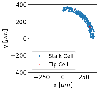
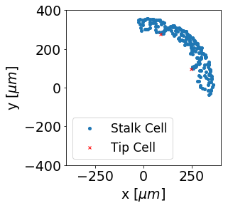
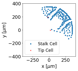
Figure 2. Positions of two tip cells (red crosses) and 200 stalk cells (blue dots) at times $T=0$ s, $T=400$ s, and $T=1600$ s.

The protein concentrations are shown in Figure 4. As the diffusion coefficient for VEGF is much larger than the reaction rate $s_{V}$, the concentration of the VEGF protein becomes uniform in the large-time limit. The DLL4, MMP, and uPA proteins are produced by the tip cells and hence follow their paths. The corresponding concentrations increase with the availability of VEGF and decrease due to consumption by the stalk cells or by getting exhausted from breaking down the fibrin matrix or the boundary membrane. Since the diffusion is slow, the changes in the concentration are local up to time $T=1600$ s.

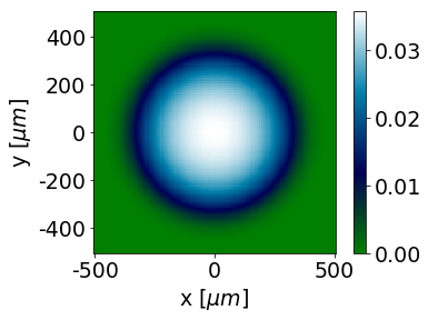
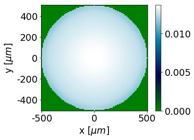
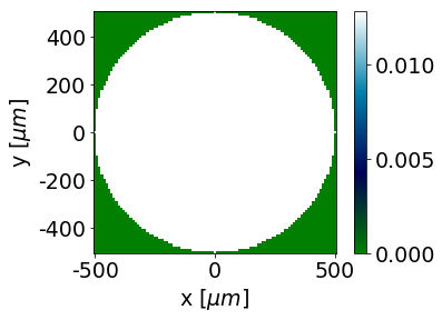
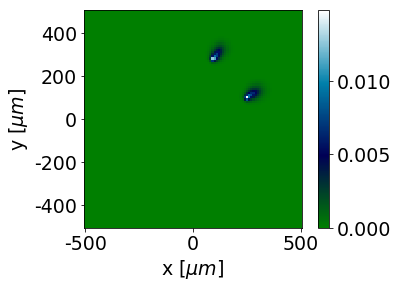
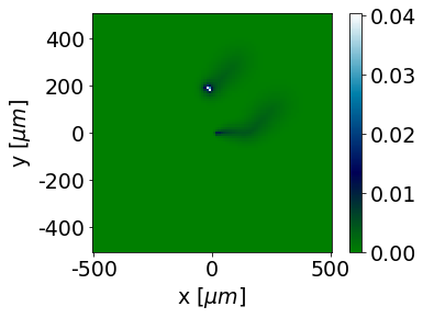
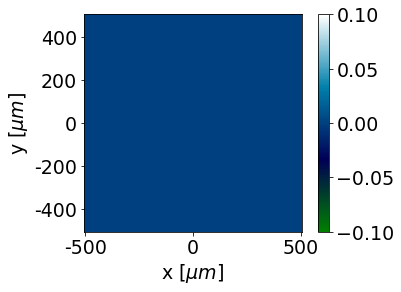
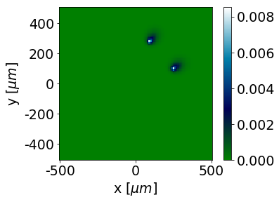
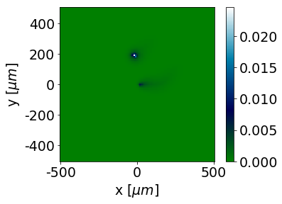
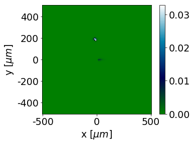
Figure 3. Concentrations of the proteins VEGF (first row), DLL4 (second row), MMP (third row), and uPA (last row) at times $T=0$ s (left column), $T=400$ s (middle column), and $T=1600$ s (right column).

We present the volume fractions of the basement membrane, fibrin matrix, and extracellular fluid in Figure 3. The membrane and fibrin matrix are degraded by the MMP and uPA proteins, thus increasing the volume fraction of the extracellular fluid. As both proteins are produced by the tip cells, the degradation follows their paths.

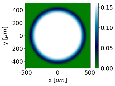
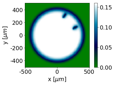
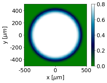
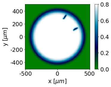
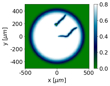
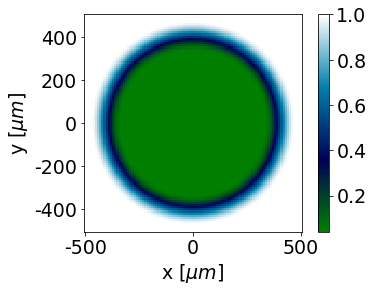
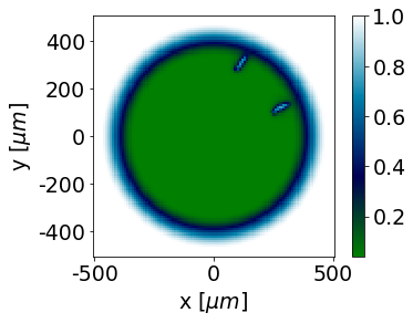
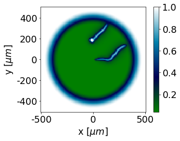
Figure 4. Volume fractions of the basement membrane (first row), fibrin matrix (second row), and extracellular fluid (last row) at times $T=0$ s (left column), $T=400$ s (middle column), and $T=1600$ s (right column).

Summarizing, we see that the model successfully describes the formation of premature sprouts. The experiments from [2] for dermal endothelial cells show that the in vitro angiogenesis sprouting qualitatively well agrees with the numerical tests. Clearly, the proposed system of equations models only a very small number of biological processes, chemical reactions, and signal proteins, and more realistic results can be only expected after taking into account more biological modeling details. Still, the onset of vessel formation is well illustrated by our simple model.

Appendix A Regularity results for elliptic and parabolic equations

Let ${\mathcal{D}}\subset{\mathbb{R}}^{m}$ ($m\geq 1$) be a bounded domain.

Theorem 18 ([22], Section IV.2, Theorem 4).

Let $\partial{\mathcal{D}}\in C^{k+2}$ and $f\in H^{k}({\mathcal{D}})$ for $k\geq 0$. Let $u\in H^{1}({\mathcal{D}})$ be a weak solution to

$$\Delta u=f\quad\mbox{in }{\mathcal{D}},\quad\nabla u\cdot\nu=0\quad\mbox{on }\partial{\mathcal{D}}.$$

Then $u\in H^{k+2}({\mathcal{D}})$, and there exists a constant $C>0$ not depending on $u$ or $f$ such that

$$\|u\|_{H^{k+2}({\mathcal{D}})}\leq C\big{(}\|f\|_{H^{k}({\mathcal{D}})}+\|u\|_{L^{2}({\mathcal{D}})}\big{)}.$$

The following regularity results hold for the parabolic problem

(23) $$\partial_{t}u-\operatorname{div}(a(x,t)\nabla u)=f\ \mbox{in }{\mathcal{D}},\ t>0,$$

$$a(x,t)\nabla u\cdot\nu=0\ \mbox{on }\partial{\mathcal{D}},\quad u(0)=u^{0}\ \mbox{in }{\mathcal{D}}.$$

Theorem 19 ([27], Section II.3, Theorem 3.3).

Let $a\in L^{\infty}(Q_{T})$ be such that $a(x,t)\geq a_{0}>0$ for all $(x,t)\in\overline{{\mathcal{D}}}\times[0,T]$, $f\in L^{2}(Q_{T})$, and $u^{0}\in H^{1}({\mathcal{D}})$. Then there exists a unique weak solution to (23) such that $u\in C^{0}([0,T];H^{1}({\mathcal{D}}))$, $\partial_{t}u\in L^{2}(Q_{T})$, and there exists a constant $C>0$, not depending on $a$, $u$, $u^{0}$, or $f$, such that

$$\|u\|_{L^{\infty}(0,T;H^{1}({\mathcal{D}}))}+\|\partial_{t}u\|_{L^{2}(Q_{T})}\leq C\big{(}\|f\|_{L^{2}(Q_{T})}+\|u^{0}\|_{H^{1}({\mathcal{D}})}\big{)}.$$

Proof.

The a priori estimate is a consequence of the proof of [27, Theorem 3.3]. ∎

Let $\alpha$, $\beta\in(0,1]$. The space $C^{\alpha,\beta}(\overline{{\mathcal{D}}}\times[0,T])$ consists of all functions $u:\overline{{\mathcal{D}}}\times[0,T]\to{\mathbb{R}}$ such that there exists $C>0$ such that for all $(x,t)$, $y,s)\in\overline{{\mathcal{D}}}\times[0,T]$,

$$|u(x,t)-u(y,s)|\leq C(|x-y|^{\alpha}+|s-t|^{\beta})\quad\mbox{for all }(x,t),\,(y,s)\in\overline{{\mathcal{D}}}\times[0,T].$$

The space $C^{k+\beta}(\overline{{\mathcal{D}}})$ is the space of all functions $u\in C^{k}(\overline{\mathcal{D}})$ such that $\mathrm{D}^{k}u$ is Hölder continuous with index $\beta>0$.

Theorem 20 ([20], Theorem 1.2).

Let $\beta\in(0,1)$, $\partial{\mathcal{D}}\in C^{1+\beta}$, $a\in C^{\beta,\beta/2}(\overline{{\mathcal{D}}}\times[0,T])$ be such that $a(x,t)\geq a_{0}>0$ for all $(x,t)\in\overline{{\mathcal{D}}}\times[0,T]$, $f\in L^{\infty}(0,T;L^{\infty}({\mathcal{D}}))$, and $u^{0}\in C^{1+\beta}(\overline{\mathcal{D}})$ be such that $a(x,t)\nabla u_{0}\cdot\nu=0$ on $\partial{\mathcal{D}}$. Furthermore, let $u\in C^{0}([0,T];L^{2}({\mathcal{D}}))\cap L^{2}(0,T;H^{1}({\mathcal{D}}))$ be a weak solution to (23). Then there exists a constant $C_{\beta}>0$, only depending on the data, such that

$$\|u\|_{C^{1+\beta,(1+\beta)/2}(\overline{{\mathcal{D}}}\times[0,T])}\leq C_{\beta}.$$

Theorem 21 ([18], Section IV.9, Theorem 9.1).

Let $\partial{\mathcal{D}}\in C^{2}$, $q>3$, $T>0$, $a\in C^{0}(\overline{{\mathcal{D}}}\times[0,T])$ be such that $a(x,t)\geq a_{0}>0$ for all $(x,t)\in\overline{{\mathcal{D}}}\times[0,T]$, $f\in L^{q}(0,T;L^{q}({\mathcal{D}}))$, $u^{0}\in W^{2,q}({\mathcal{D}})$ be such that $a(x,t)\nabla u^{0}\cdot\nu=0$ on $\partial{\mathcal{D}}$. Then there exists a unique strong solution $u\in L^{q}(0,T;W^{2,q}({\mathcal{D}}))$ to (23) satisfying $\partial_{t}u\in L^{q}(0,T;L^{q}({\mathcal{D}}))$, and there exists a constant $C>0$, not depending on $u$, $f$, or $u_{0}$, such that

$$\|u\|_{L^{q}(0,T;W^{2,q}({\mathcal{D}}))}+\|\partial_{t}u\|_{L^{q}(0,T;L^{q}({\mathcal{D}}))}\leq C\big{(}\|f\|_{L^{q}(0,T;L^{q}({\mathcal{D}}))}+\|u_{0}\|_{W^{2,q}({\mathcal{D}})}\big{)}.$$

Theorem 22 ([18], Section V.5, Theorem 5.4).

Let $\beta\in(0,1)$, $\partial{\mathcal{D}}\in C^{2+\beta}$, $T>0$, $a_{ij}$, $b_{i}$, $c\in C^{\beta,\beta/2}(\overline{{\mathcal{D}}}\times[0,T])$ be such that $a_{ij}(x,t)\geq a_{0}>0$ for all $(x,t)\in\overline{{\mathcal{D}}}\times[0,T]$ for $i,j=1,\ldots,m$, $f\in C^{\beta,\beta/2}(\overline{{\mathcal{D}}}\times[0,T])$, and $u^{0}\in C^{2+\beta}(\overline{\mathcal{D}})$ be such that $\nabla u_{0}\cdot\nu=0$ on $\partial{\mathcal{D}}$. Then there exists a unique classical solution $u\in C^{2+\beta,1+\beta}(\overline{{\mathcal{D}}}\times[0,T])$ to

$$\partial_{t}u-\sum_{i,j=1}^{m}a_{ij}(x,t)\frac{\partial^{2}u}{\partial x_{i}\partial x_{j}}+b(x,t)\cdot\nabla u+c(x,t)u=f\quad\mbox{in }{\mathcal{D}},\ t>0,$$

$$\nabla u\cdot\nu=0\quad\mbox{on }\partial{\mathcal{D}},\ t>0,\quad u(0)=u^{0}\quad\mbox{in }{\mathcal{D}},$$

and there exists a constant $C>0$, not depending on $u$, $f$, or $u_{0}$, such that

$$\|u\|_{C^{2+\beta,1+\beta}(\overline{{\mathcal{D}}}\times[0,T])}\leq C\big{(}\|f\|_{C^{\beta;\beta/2}(\overline{{\mathcal{D}}}\times[0,T])}+\|u_{0}\|_{C^{2+\beta}(\overline{\mathcal{D}})}\big{)}.$$

Appendix B Model parameters and constants

The model parameters and constants are taken from [2]. For the convenience of the reader, we collect here the expressions:

$$\alpha_{0} =\frac{b_{i}R_{c}^{3}}{F_{i}\mu},$$

$$\gamma(x,t) =\frac{0.1b_{i}F_{i}(1-f_{E}(x,t))}{\rho_{B}f_{B}(x,t)+\rho_{F}f_{F}(x,t)+\rho_{E}f_{E}(x,t)},$$

$$\lambda(x,t) =\frac{4^{3}b_{i}F_{i}\widetilde{\lambda}}{30}(1-f_{E}(x,t))\bigg{(}\frac{1}{2}-f_{E}(x,t)\bigg{)}f_{E}(x,t),$$

$$M_{i}^{k}(x,t) =\sum_{j=1}^{2}\sum_{\ell=1}^{N_{j}}\frac{F_{i}^{2}}{20\pi^{2}R_{c}^{4}}(1-f_{E}(x,t))\exp\bigg{(}\frac{-|X_{i}^{k}-X_{j}^{\ell}|}{R_{c}}\bigg{)}$$

$$\phantom{xx}{}-\frac{2\sqrt{2}}{\pi}\bigg{(}\frac{\max\{0,R_{c}-0.5|X_{i}^{k}-X_{j}^{\ell}|\}}{R_{c}}\bigg{)}^{5/2},$$

$$v_{i}^{k} =\sum_{j=1}^{2}\sum_{\ell=1}^{N_{j}}\frac{F_{i}^{2}}{20\pi^{2}R_{c}^{4}}(1-f_{E}(x,t))\exp\bigg{(}\frac{-|X_{i}^{k}-X_{j}^{\ell}|}{R_{c}}\bigg{)},$$

$$z_{i}^{k} =\frac{v_{i}^{k}}{|v_{i}^{k}|}.$$

The parameters are chosen as in the following table; see [2, Appendix].

	Value	Unit		Value	Unit		Value	Unit
$b_{i}$	0.02	$\textrm{s}^{-1}$	$D_{V}^{E}$	10	$\mu\textrm{m}^{2}\textrm{s}^{-1}$	$r_{D}$	10	$\mu\textrm{m}^{3}\textrm{s}^{-1}$
$F_{i}$	1000	nN	$D_{D}^{B}$	0.51	$\mu\textrm{m}^{2}\textrm{s}^{-1}$	$r_{M}$	10	$\mu\textrm{m}^{3}\textrm{s}^{-1}$
$\mu$	0.2	–	$D_{D}^{F}$	1.02	$\mu\textrm{m}^{2}\textrm{s}^{-1}$	$r_{U}$	10	$\mu\textrm{m}^{3}\textrm{s}^{-1}$
$\widetilde{\lambda}$	15	–	$D_{D}^{E}$	0.051	$\mu\textrm{m}^{2}\textrm{s}^{-1}$	$s_{V}$	0.024	$\mu\textrm{m}^{3}\textrm{s}^{-1}$
$R_{c}$	11.25	$\mu\textrm{m}$	$D_{M}^{B}$	1.23	$\mu\textrm{m}^{2}\textrm{s}^{-1}$	$s_{D}$	0.024	$\mu\textrm{m}^{3}\textrm{s}^{-1}$
$\rho_{B}$	$1.06\cdot 10^{-3}$	$\textrm{ng}\mu\textrm{m}^{-3}$	$D_{M}^{F}$	2.46	$\mu\textrm{m}^{2}\textrm{s}^{-1}$	$s_{M}$	0.024	$\textrm{s}^{-1}$
$\rho_{F}$	$1.06\cdot 10^{-3}$	$\textrm{ng}\mu\textrm{m}^{-3}$	$D_{M}^{E}$	0.123	$\mu\textrm{m}^{2}\textrm{s}^{-1}$	$s_{U}$	0.024	$\textrm{s}^{-1}$
$\rho_{E}$	$0.9933\cdot 10^{-3}$	$\textrm{ng}\mu\textrm{m}^{-3}$	$D_{U}^{B}$	0.53	$\mu\textrm{m}^{2}\textrm{s}^{-1}$	$s_{B}$	1.21	$\mu\textrm{m}^{3}\textrm{ng}^{-1}\textrm{s}^{-1}$
$D_{V}^{B}$	100	$\mu\textrm{m}^{2}\textrm{s}^{-1}$	$D_{U}^{F}$	1.06	$\mu\textrm{m}^{2}\textrm{s}^{-1}$	$s_{F}$	1.21	$\mu\textrm{m}^{3}\textrm{ng}^{-1}\textrm{s}^{-1}$
$D_{V}^{F}$	200	$\mu\textrm{m}^{2}\textrm{s}^{-1}$	$D_{U}^{E}$	0.053	$\mu\textrm{m}^{2}\textrm{s}^{-1}$

References

- [1] R. Blanco and H. Gerhardt. VEGF and notch in tip and stalk cell selection. Cold Spring Harb. Perspect. Med. 3 (2013), a006569.
- [2] F. Bookholt, H. Monsuur, S. Gibbs, and F. Vermolen. Mathematical modelling of angiogenesis using continuous cell-based models. Biomech. Model. Mechanobiol. 15 (2016), 1577–1600.
- [3] N. Britton and M. Chaplain. A qualitative analysis of some models of tissue growth. Math. Biosci. 113 (1993), 77–89.
- [4] H. Byrne and D. Drasdo. Individual-based and continuum models of growthing cell populations: a comparison. J. Math. Biol. 58 (2009), 657–687.
- [5] A. Carlier, L. Geris, K. Bentley, G. Carmeliet, P. Carmeliet, and H. van Oosterwyck. MOSAIC: a multiscale model of osteogenesis and sprouting angiogenesis with lateral inhibition of endothelial cells. PLOS Comput. Biol. 8 (2012), e1002724.
- [6] V. Capasso and F. Flandoli. On the mean field approximation of a stochastic model of tumour-induced angiogenesis. Europ. J. Appl. Math. 30 (2019), 619–658.
- [7] V. Capasso and D. Morale. Stochastic modelling of tumour-induced angiogenesis. J. Math. Biol. 58 (2009), 219–233.
- [8] M. Chaplain, S. McDougall, and A. Anderson. Mathematical modeling of tumor-induced angiogenesis. Ann. Rev. Biomed. Engin. 8 (2006), 233–257.
- [9] L. Corrias, B. Perthame, and H. Zaag. Global solutions of some chemotaxis and angiogenesis systems in high space dimensions. Milan J. Math. 72 (2004), 1–28.
- [10] E. Gaffney, K. Pugh, and P. Maini. Investigating a simple model for cutaneous wound healing angiogenesis. J. Math. Biol. 45 (2002), 337–374.
- [11] D. Gilbarg and N. Trudinger. Elliptic Partial Differential Equations of Second Order. Springer, Berlin, 1998.
- [12] F. Graner and J. Glazier. Simulation of biological cell sorting using a two-dimensional extended Potts model. Phys. Rev. Lett. 69 (1992), 2013–2016.
- [13] S. Hiremath, C. Surulescu, A. Zhigun, and S. Sonner. On a coupled SDE-PDE system modeling acid-mediated tumor invasion. Discrete Contin. Dyn. Sys. B 23 (2018), 2339–2369.
- [14] B. Jourdain, C. Le Bris and T. Lelièvre. Coupling PDEs and SDEs: the illustrative example of the multiscale simulation of viscoelastic flows. In: B. Engquist, O. Runborg, and P. Lötstedt (ed.s), Multiscale Methods in Science and Engineering, Lect. Notes Comput. Sci. Eng. 44, pp. 149–168. Springer, Berlin, 2005.
- [15] O. Kallenberg. Foundations of Modern Probability. 3rd edition. Springer, Cham, 2021.
- [16] J. Karatzas and S. Shreve. Brownian Motion and Stochastic Calculus. 2nd edition. Springer, New York, 1991.
- [17] P. Kloeden, S. Sonner, and C. Surulescu. A nonlocal sample dependence SDE-PDE system modeling proton dynamics in a tumor. Discrete Contin. Dyn. Sys. B 21 (2016), 2233–2254.
- [18] O. A. Ladyženskaja, V. A. Solonnikov, and N. N. Ural’ceva. Linear and Quasi-linear Equations of Parabolic Type. Amer. Math. Soc., Providence, 1968.
- [19] A. Latif. Banach contraction principle and its generalizations. In: S. Almezel, Q. H. Ansari, and M. A. Khamsi (eds.), Topics in Fixed Point Theory, pp. 33–64. Springer, Cham, 2014.
- [20] G. Lieberman. Hölder continuity of the gradient of solutions of uniformly parabolic equations with conormal boundary conditions. Ann. Mat. Pura Appl. 148 (1987), 77–99.
- [21] W. Liu and M. Röckner. Stochastic Partial Differential Equations: an Introduction. Springer, Cham, 2015.
- [22] V. P. Mikhailov. Partial Differential Equations. Mir Publishers, Moscow, 1976.
- [23] R. Nittka. Regularity of solutions of linear second order elliptic and parabolic boundary value problems on Lipschitz domains. J. Diff. Eqs. 251 (2011), 860–880.
- [24] S. Pierce. Computational and mathematical modeling of angiogenesis. Microcirculation 15 (2008), 739–751.
- [25] F. Spill, P. Guerrero, T. Alarcon, P. Maini, and H. Byrne. Mesoscopic and continuum modelling of angiogenesis. J. Math. Biol. 70 (2015), 485–532.
- [26] C. Stokes and D. Lauffenburger. Analysis of the roles of microvessel endothelial cell random motility and chemotaxis in angiogenesis. J. Theor. Biol. 152 (1991), 377–403.
- [27] R. Temam. Infinite-Dimensional Dynamical Systems in Mechanics and Physics. 2nd edition. Springer, New York, 1997.
- [28] A. Ucuzian, A. Gassman, A. East, and H. Greisler. Molecular mediators of angiogenesis. J. Burn Care Res. 31 (2010), no. 158.
- [29] F. Vermolen and A. Gefen. A semi-stochastic cell-based formalism to model the dynamics of migration of cells in colonies. Biomech. Model. Mechanobiol. 11 (2012), 183–195.
- [30] E. Zeidler. Nonlinear Functional Analysis and its Applications. Vol. II/A. Springer, New York, 1990.