Modular Conformal Calibration

Abstract

Uncertainty estimates must be calibrated (i.e., accurate) and sharp (i.e., informative) in order to be useful. This has motivated a variety of methods for recalibration, which use held-out data to turn an uncalibrated model into a calibrated model. However, the applicability of existing methods is limited due to their assumption that the original model is also a probabilistic model. We introduce a versatile class of algorithms for recalibration in regression that we call modular conformal calibration (MCC). This framework allows one to transform any regression model into a calibrated probabilistic model. The modular design of MCC allows us to make simple adjustments to existing algorithms that enable well-behaved distribution predictions. We also provide finite-sample calibration guarantees for MCC algorithms. Our framework recovers isotonic recalibration, conformal calibration, and conformal interval prediction, implying that our theoretical results apply to those methods as well. Finally, we conduct an empirical study of MCC on 17 regression datasets. Our results show that new algorithms designed in our framework achieve near-perfect calibration and improve sharpness relative to existing methods.

1 Introduction

Uncertainty estimates can inform human decisions (Pratt et al., 1995; Berger, 2013), flag when an automated decision system requires human review (Kang et al., 2021), and serve as an internal component of automated systems. For example, uncertainty informs treatment decisions in medicine (Begoli et al., 2019) and supports safety in autonomous navigation (Michelmore et al., 2018). In such settings, the benefits of accounting for uncertainty hinge on our ability to produce calibrated uncertainty estimates—e.g., of those events to which one assigns a probability of 90%, the events should indeed occur 90% of the time. A model that is not calibrated can consistently make confident predictions that are incorrect.

Many models, such as neural networks (Guo et al., 2017) and Gaussian processes (Rasmussen, 2003; Tran et al., 2019), achieve high accuracy but have poorly calibrated or absent uncertainty estimates. In other cases, a pretrained model is released for wide use and it is difficult to guarantee that it will produce calibrated uncertainty estimates in new settings (Zhao et al., 2021). This leads us to the question: how can we safely deploy models with high predictive value but poor or absent uncertainty estimates?

These challenges have motivated work on recalibration, whereby a model with poor uncertainty estimates is transformed into a probabilistic model that outputs calibrated probabilities (Kuleshov et al., 2018; Vovk et al., 2020; Niculescu-Mizil & Caruana, 2005; Chung et al., 2021). Recalibration methods are attractive because they require only black-box access to a given model and can return well-calibrated probabilistic predictions.

However, calibration is not the only goal of probabilistic models. It is also important for a probabilistic model to predict sharp (i.e., low variance) distributions to convey more information. Furthermore, recalibration methods need to be data efficient to calibrate models in data poor regimes.

In this paper, we introduce modular conformal calibration (MCC), a class of algorithms that unifies existing recalibration methods and gives well-behaved distribution predictions from any model. Our main contributions are:

1. We introduce modular conformal calibration, a class of algorithms for recalibration in regression, which can be applied to recalibrate almost any regression model. MCC unifies isotonic calibration (Kuleshov et al., 2018), conformal calibration (Vovk et al., 2020), and conformal interval prediction (Vovk et al., 2005) under a single theoretical framework, and additionally leads to new algorithms.

2. We provide finite-sample calibration guarantees, showing that MCC can achieve $\epsilon$ calibration error with $O(1/\epsilon)$ samples. These results also apply to the aforementioned recalibration methods that MCC unifies.

3. We conduct an empirical study on 17 datasets to compare the performance of recalibration methods in practice. We find that new algorithms within our framework outperform existing methods in terms of both sharpness and proper scoring rules.

2 Background

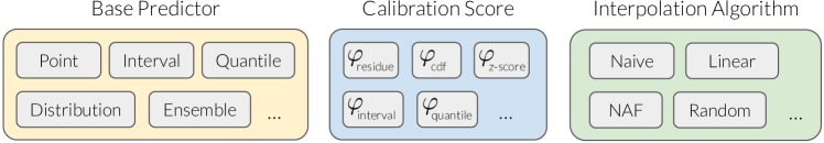
Figure 1: A combination of the three components defines a modular conformal calibration algorithm.

Given an input feature vector $x\in{\mathcal{X}}$ (e.g., a satellite image), we want to predict a label $y\in{\mathcal{Y}}$ (e.g., the temperature tomorrow). We consider regression problems where ${\mathcal{Y}}={\mathbb{R}}$. We assume there is a true distribution ${\mathbb{F}}_{XY}$ over ${\mathcal{X}}\times{\mathcal{Y}}$, and we have access to $n$ i.i.d. examples $(X_{i},Y_{i})\sim{\mathbb{F}}_{XY}$.

Given a feature vector $x$, our goal is to predict the conditional distribution of $Y$ given $X=x$, denoted ${\mathbb{F}}_{Y\mid x}$. A distribution predictor is a function $H:{\mathcal{X}}\to{\mathcal{F}}({\mathcal{Y}})$ that takes a feature vector $x$ as input and returns $H[x]$, a cumulative distribution function (CDF) over ${\mathcal{Y}}$. Note that $H[x]\in{\mathcal{F}}({\mathcal{Y}})$ is a function, intended to approximate ${\mathbb{F}}_{Y\mid x}$ by mapping any input $y\in{\mathcal{Y}}$ to a value $H[x](y)$ in $[0,1]$.

We consider a two-stage process to learn a distribution predictor from data. In the first stage, we train the base predictor $f:{\mathcal{X}}\to{\mathcal{R}}$, which maps a feature vector $x$ to a prediction in a space ${\mathcal{R}}$. The base predictor can be any model (e.g., neural network, support vector machine) and the prediction can be of any type; for example, $f$ could give a point prediction for the mean of ${\mathbb{F}}_{Y\mid x}$ (i.e., ${\mathcal{R}}={\mathbb{R}}$) or $f$ could give an interval prediction that is likely to contain $Y$ (i.e., ${\mathcal{R}}={\mathbb{R}}^{2}$). Alternatively, $f$ could predict a Gaussian distribution that approximates the distribution of the label (i.e., ${\mathcal{R}}={\mathcal{F}}({\mathcal{Y}})$).

Regardless of the base predictor we choose, the second step is to recalibrate the base predictor: we translate the base predictor $f$ into a calibrated distribution predictor $H$. We construct $H$ by fitting a wrapper function around $f$, meaning that $H[x]$ only depends on $x$ via the prediction $f(x)$.

We focus on the second stage, that of recalibration. For those interested in which base predictors yield the best recalibrated predictors, see Section 6 for an empirical study.

Example 1 (Linear Regression).

Consider a linear regression problem where $Y_{i}=\beta^{\top}X_{i}+\epsilon_{i}$ for $X_{i}\in{\mathbb{R}}^{d}$, $\beta\in{\mathbb{R}}^{d}$, and $\epsilon_{i}\in{\mathbb{R}}$ distributed i.i.d. with known CDF ${\mathbb{F}}_{\epsilon}$. Imagine we are given a base predictor $f(x)=\beta^{T}x$ that perfectly predicts the mean of ${\mathbb{F}}_{Y\mid x}$. Then we can construct a perfect distribution predictor $H[x]:{\mathcal{Y}}\rightarrow[0,1]$ by defining:

$$H[x](y):={\mathbb{F}}_{\epsilon}(y-f(x))={\mathbb{F}}_{Y\mid x}(y)$$

Note that the CDF prediction $H[x]$ only depends on $x$ through the point prediction $f(x)$, but still gives perfect distribution predictions.

Calibration

Optimally, the distribution predictor $H$ will output for each value $x$ the true conditional CDF, $H[x]={\mathbb{F}}_{Y\mid x}$, as in Example 1. However, many feature vectors $x$ only appear once in our data, making it impossible to learn a perfect distribution predictor $H$ from data without additional assumptions (such as the assumptions of linearity and i.i.d. noise in Example 1). Instead of making additional assumptions, we instead aim for calibration, a weaker property than perfect distribution prediction that can be obtained in practice.

Recall that for any random variable $Y$, the probability integral transform ${\mathbb{F}}_{Y}(Y)$ obtained by evaluating the CDF with random input $Y$ follows a standard uniform distribution. We should expect the same behavior from our predicted CDFs; we should observe that $H[X](Y)$ also follows a standard uniform distribution. For example, the observed label should be greater than the predicted 95th percentile for approximately 5% of examples.

Definition 1.

Given a distribution predictor $H:{\mathcal{X}}\to{\mathcal{F}}({\mathcal{Y}})$, we say that $H$ is calibrated if $H[X](Y)$ follows a standard uniform distribution. Formally, $H$ is calibrated if

$$\Pr(H[X](Y)\leq p)=p,\quad\text{for all }p\in[0,1]$$ (1)

Similarly, for a value $\epsilon\geq 0$, we say that $H$ is $\epsilon$-calibrated if Equation (1) is only violated by at most $\epsilon$:

$$\Pr(H[X](Y)\leq p)\in p\pm\epsilon,\quad\textrm{for all }p\in[0,1]$$ (2)

Calibration is a necessary but not sufficient condition for making good distribution predictions. Note that a distribution predictor $H[x]={\mathbb{F}}_{Y}$ that ignores $x$ and returns the marginal cdf for $Y$ will be calibrated, but not useful. Thus, distribution predictions should be as sharp (i.e., highly concentrated) as possible, conditioned on being calibrated.

Related Work

Post-hoc uncertainty quantification is an active field of research. Platt scaling (Platt et al., 1999) and isotonic regression (Niculescu-Mizil & Caruana, 2005) are popular methods for recalibrating binary classifiers. Platt scaling fits a logistic regression model to the scores given by a model, and isotonic regression learns a nondecreasing map from scores to the unit interval. Quantile regression (Romano et al., 2019; Chung et al., 2020, e.g.,) simultaneously estimates multiple quantiles of the label distribution, often via the pinball loss, which can then be combined to construct calibrated distribution predictions.

Isotonic calibration (Kuleshov et al., 2018) is an effective strategy for recalibrating a base predictor that already makes distribution predictions. Isotonic calibration computes the empirical quantiles (i.e., $f[X_{i}](Y_{i})$) of a distribution predictor on the calibration dataset, and uses isotonic regression to adjust the empirical quantiles so that they are uniform on $[0,1]$. Conformal calibration (Vovk et al., 2020) is similar to isotonic calibration, except it uses a randomized function to adjust the empirical quantiles instead of isotonic regression. This yields strong calibration guarantees, at the cost of discontinuous and randomized distribution predictions.

Conformal prediction (Vovk et al., 2005) is a general approach to uncertainty quantification that produces prediction sets (i.e., interval predictions) with guaranteed coverage, instead of distribution predictions. In the context of these prediction sets, some prior work has also studied the connection between conformal prediction and calibration (Lei et al., 2018; Gupta et al., 2020; Angelopoulos & Bates, 2021). Our work builds on isotonic calibration, conformal calibration, and conformal prediction to construct novel recalibration algorithms for arbitrary base predictors.

3 Modular Conformal Calibration

In this section, we introduce a new class of recalibration procedures and provide calibration guarantees for this class of algorithms. We begin with a simple example in which we recalibrate a point predictor, then we generalize this reasoning to introduce modular conformal calibration. We conclude this section by enumerating design choices our framework introduces.

3.1 Warm-up

We start with a simple example to introduce the main idea. In this example, we turn a point predictor into a calibrated distribution predictor.

1. Suppose we have a base predictor $f:{\mathcal{X}}\to{\mathbb{R}}$ that uses a satellite image $X$ to produce a point estimate for the temperature the following day $Y$. Additionally, we are given a dataset $(X_{1},Y_{1}),\dots,(X_{n},Y_{n})$ where we observe both the satellite image and temperature. Now, given a new satellite image $X_{*}$, we want to predict the (unobserved) temperature $Y_{*}$. It is important for us to quantify our uncertainty if this prediction will inform a decision—we will likely behave differently if the temperature is certain to be within 2 degrees of our estimate, versus if it could differ by 20 degrees.

2. We can apply the residue function $\varphi(f(x),y)=y-f(x)$ to our predictions, giving $S_{1}=Y_{1}-f(X_{1}),\cdots,S_{n}=Y_{n}-f(X_{n})$; if we knew the label $Y_{*}$, we could also apply the residue score to our test example to compute a residue $S_{*}=Y_{*}-f(X_{*})$. If the data is i.i.d. then the residues are also i.i.d. random variables.

3. We can consider how large or small $S_{*}$ is among the set of residues $\{S_{1},\cdots,S_{n}\}$. Intuitively, because of the i.i.d. assumptions, $S_{*}$ is equally likely to be the smallest, 2nd smallest, …, largest element. Formally, if we define the ranking function $q$ as:

   $$q(t):=\frac{1}{n}\sum_{i=1}^{n}\mathds{1}\{t\leq S_{i}\}\$$

   then up to discretization error

   $$\Pr[q(S_{*})\leq c]\approx c,\forall c\in[0,1]$$ (3)

In fact, Eq.(3) is exactly the definition of calibration so the reasoning above proves that the CDF predictor $H[x](y)=q(\varphi(f(x),y))$ is approximately calibrated. We also have to show that $H[x]$ is a CDF. This is easy to prove, as $q(\varphi(f(x),y))$ is a nondecreasing function in $y$. We conclude that $H$ is an approximately calibrated CDF predictor.

3.2 Components of a Recalibration Algorithm

Algorithm 1 Modular Conformal Calibration

  Input: base predictor $f:{\mathcal{X}}\to{\mathcal{R}}$, calibration score $\varphi:{\mathcal{R}}\times{\mathcal{Y}}\to{\mathbb{R}}$ and interpolation algorithm $\psi$

  Input: calibration dataset $(X_{1},Y_{1}),\cdots,(X_{n},Y_{n})$

  Compute calibration scores $S_{i}=\varphi(f(X_{i}),Y_{i})$ for $i=1,\dots,n$

  Run the interpolation algorithm $q=\psi\left(S_{1},\cdots,S_{n}\right)$

  Return: the CDF predictor $H[x](y)=q(\varphi(f(x),y)$

We organize the design choices within modular conformal calibration into three decisions:

1. Base predictor. In the first step, we choose a base predictor. This can be any prediction function $f:{\mathcal{X}}\to{\mathcal{R}}$. There are no restrictions on the prediction space ${\mathcal{R}}$, as long as we can define a compatible calibration score. The only requirement is that $f$ is not learned on the calibration dataset $(X_{1},Y_{1}),\cdots,(X_{n},Y_{n})$, but it could be learned on any different dataset. In the previous example, the base predictor is a point prediction function.

2. Calibration score. In the second step, we choose a calibration score, which is any function $\varphi:{\mathcal{R}}\times{\mathcal{Y}}\to{\mathbb{R}}$ that is monotonically strictly increasing in $y$. In the previous example, the calibration score is the residue $\varphi(f(x),y)=y-f(x)$. Intuitively, the calibration score should reflect how large $y$ is relative to our prediction $f(x)$. We can then compute the calibration score for each sample in the training set $S_{i}=\varphi(X_{i},Y_{i});i=1,\cdots,n$. For convenience of computing rankings, we sort the scores into $S_{(1)}\leq S_{(2)}\leq\cdots\leq S_{(n)}$.

3. Interpolation algorithm. Finally we need a map from the calibration score to the final CDF output. In example 1 we constructed an interpolation map (the function $q$) by mapping any score in $(S_{(i-1)},S_{(i)}]$ to $i/n$. The interpolation algorithm we use here is a very simple step function. However, the resulting CDFs are not continuous which may be inconvenient (e.g., if we want to compute the log likelihood).

More generally we can use any interpolation algorithm: let ${\mathcal{Q}}$ be the set of monotonically non-decreasing functions ${\mathbb{R}}\to[0,1]$. An interpolation algorithm is a map $\psi:{\mathbb{R}}^{n}\to{\mathcal{Q}}$. An interpolation algorithm maps the calibration scores $S_{1},\dots,S_{n}$ to a function $q$ such that $q(S_{1}),\dots,q(S_{n})$ are approximately evenly spaced on the unit interval.

Definition 2.

An interpolation function $\psi:{\mathbb{R}}^{n}\to{\mathcal{Q}}$ is $\lambda$-accurate if for any distinct inputs $(u_{1},u_{2},\dots,u_{n})\in{\mathbb{R}}^{n}$ the function $q=\psi(u_{1},u_{2},\cdots,u_{n})$ maps the $i$-th smallest input $u_{(i)}$ close to $i/(n+1)$:

$$q\left(u_{(i)}\right)\in\frac{i\pm\lambda}{n+1},\quad\text{for all }i=1,\dots,n$$ (4)

If $\psi$ is a randomized function, then the statement is quantified by almost surely.

If a $\lambda$-accurate interpolation algorithm is applied to calibration scores computed on a held-out dataset, the function $q\circ\varphi$ will be approximately calibrated on that dataset. We can write the full process for making a CDF prediction as:

$$H[x](y)=\underbrace{q(\varphi(f(x),y))}_{\text{prediction for}\Pr(Y\leq y\mid X=x)}$$ (5)

This three step process of applying a base predictor $f$, calibration score $\varphi$, and interpolation function $q$ (learned by an interpolation algorithm $\psi$) is detailed in Algorithm 1 and illustrated in Figure 1. Now, we formalize the intuition that $H$ will be calibrated into a formal guarantee.

Theorem 1.

For any base predictor $f$, calibration score $\varphi$, and $\lambda$-accurate interpolation algorithm $\psi$ such that the random variable $\varphi(f(X),Y)$ is absolutely continuous, Algorithm 1 is $\frac{1+\lambda}{n+1}$-calibrated.

See Appendix C for a proof of Theorem 1. Similar to conformal interval prediction, there is a rather mild regularity assumption: $\varphi(f(X),Y)$ has to be absolutely continuous, i.e. two i.i.d. samples $(X_{1},Y_{1})$ and $(X_{2},Y_{2})$ almost never have the same score $\varphi(f(X_{1}),Y_{1})\neq\varphi(f(X_{2}),Y_{2})$. In our warm-up example in Section 3.1, this condition requires that two samples $(X_{1},Y_{1})$, $(X_{2},Y_{2})$ almost never have exactly the same residue $Y_{1}-f(X_{1})\neq Y_{2}-f(X_{2})$.

4 Choosing a Recalibration Algorithm

In this section, we describe natural choices for the calibration score and interpolation algorithm, given different base predictors. A main motivation for introducing the modular conformal calibration framework is to make it easy to develop new recalibration procedures. Any pairing of the calibration scores and interpolation algorithms described in this section results in a recalibration algorithm with the finite-sample calibration guarantee given by Theorem 1.

4.1 The Base Predictor

In some cases the base predictor will be fixed, such as when fine-tuning a pretrained model to be calibrated in a new setting. In other cases, we have end-to-end control of the training process. In these cases, we must answer the question: Which base predictor should I train to get the best calibrated distribution predictor?

An obvious choice is to learn a distribution predictor as the base predictor then recalibrate if needed. However, there is no guarantee that this will produce better results than learning a different type of base predictor (e.g., one of the prediction types in Table 1) then recalibrating. In fact, in our experiments we find that even when learners are of similar power, distribution predictors are not necessarily the most effective choice of base predictor (see Section 6).

Prediction Type	Output Space (${\mathcal{R}}$)	Interpretation
Point	${\mathbb{R}}$	e.g. estimate of the mean.
Interval	${\mathbb{R}}^{2}$	Interval is $[f_{1}(x),f_{2}(x)]$.
Quantile	${\mathbb{R}}^{K}$	$f_{k}(x)$ predicts a quantile $\alpha_{k}\in(0,1)$.
Distribution	${\mathcal{F}}({\mathbb{R}})$	$f[x]$ is a predicted CDF for $y$.
Ensemble	${\mathcal{R}}_{1}{\times}{\cdots}{\times}R_{K}$	Each $f_{k}$ is the prediction of a model $k$.

Table 1: A collection of common prediction types.

4.2 The calibration score

In this section, we introduce calibration scores for a few prediction types (see Table 1) to illustrate the role of the calibration score. Intuitively, a good calibration score should measure how large $y$ is relative to the prediction. Recall that the calibration score $\varphi:{\mathcal{R}}\times{\mathcal{Y}}\to{\mathbb{R}}$ can be any function that is non-decreasing in $y$. A poor choice of calibration score still guarantees calibration (see Theorem 1), but can harm other metrics such as sharpness or NLL. Additional calibration scores for quantile prediction and ensemble prediction can be found in Appendix A.

Point Prediction

A natural calibration score for point predictors is the residue $\varphi_{\text{residue}}(x,y)=y-f(x)$.

Interval Prediction

For interval predictors, a natural choice for the calibration score is the residue divided by the interval size $\varphi_{\text{interval}}(x,y)=(y-f_{1}(x))/(f_{2}(x)-f_{1}(x))$. Intuitively, if $y$ equals the predicted upper bound $f_{2}(x)$, then the calibration score is $1$; if $y$ equals the lower bound $f_{1}(x)$ then the calibration score is $0$. The calibration scores of all other $y$ are linear interpolations of these two.

Distribution Prediction

Given a distribution prediction, i.e. a map $f:{\mathcal{X}}\to{\mathcal{F}}({\mathcal{Y}})$ two natural choices for the calibration score are

$$\varphi_{\text{cdf}}(x,y) =f[x](y)$$

$$\varphi_{\text{z-score}}(x,y) =(y-\mathrm{mean}(f(x)))/\mathrm{std}(f(x))$$

Numerical stability is a practical issue for $\varphi_{\text{cdf}}$. When $y$ is small or large, the calibration score may be the same for different $y$ due to rounding with finite numerical precision. Empirically, $\varphi_{\text{z-score}}$ has better numerical stability and often better performance.

4.3 The Interpolation Algorithm

Lastly, we discuss the choice of interpolation algorithm. We illustrate a simple linear interpolation algorithm, a randomized interpolation algorithm with strong theoretical guarantees, and a more complex approach using neural autoregressive flows. Recall that an interpolation algorithm is a function $\psi$ that maps a vector $(u_{1},\dots,u_{n})$ to a non-decreasing function $q$ such that $q(u_{1}),\dots,q(u_{n})$ are approximately evenly spaced on the unit interval. Recall also that we write $u_{(i)}$ to denote the $i$-th smallest input.

Naive Discretization

As we discussed, the interpolation algorithm in Example 1 is

$$q_{\text{naive}}(u)=i/n,\quad\text{if }u\in[u_{(i)},u_{(i+1)})$$ (6)

While simple, the resulting CDF is not continuous, making quantities such as the log-likelihood undefined. It is also not $0$-accurate (recall Definition 2). For better performance we need more sophisticated interpolation algorithms.

Linear

Linear interpolation is a simple way to get a continuous CDF function with a density.

$$q_{\mathrm{linear}}(u)=\frac{i+(u-u_{(i)})/(u_{(i+1)}-u_{(i)})}{n+1}$$

for $u\in[u_{(i)},u_{(i+1)})$. A piecewise linear CDF is differentiable almost everywhere, so the log likelihood and density function are well-defined almost everywhere. Linear interpolation can perfectly fit any monotonic sequence, and is therefore $0$-accurate.

Neural Autoregressive Flow (NAF)

To achieve even better smoothness properties, we can use a neural autoregressive flow (NAF), which is a class of deep neural networks that can universally approximate bounded continuous monotonic functions (Huang et al., 2018). The benefit of using a NAF is that the resulting CDF will be more “smooth”. In fact, if we use a differentiable activation function for the NAF network (such as sigmoid rather than ReLU), then NAF represents smooth CDF functions that are differentiable everywhere.

The short-coming is that NAF can only represent arbitrary monotonic functions (and hence be a $0$-accurate interpolation algorithm) if the network is infinitely wide. In our experiments, a network with 200 units is sufficient to push the errors below numerical precision.

Random

Finally there is an interpolation algorithm that uses randomization, which would recover the algorithm in (Vovk et al., 2020). Let $U$ be uniform on $[0,1]$.

$$q_{\mathrm{random}}(u)=(i+U)/(n+1)\qquad\text{if }u\in[u_{(i)},u_{(i+1)})$$

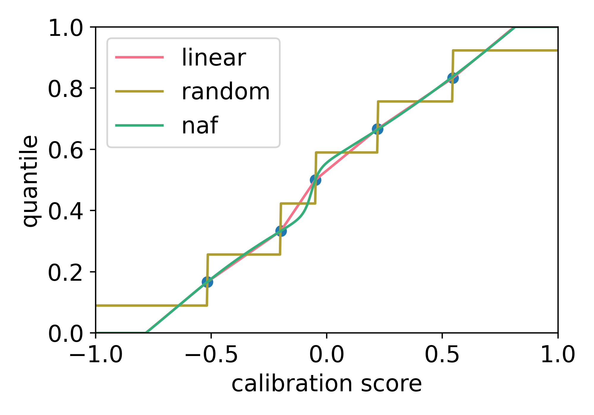
Calibration error Log-likelihood Computation Random Perfect ($\color[rgb]{0,1,0}{+}$) Undefined ($\color[rgb]{1,0,0}{-}$) Fast ($\color[rgb]{0,1,0}{+}$) Linear $O(1/T)$ ($\color[rgb]{1,1,0}$) Well defined ($\color[rgb]{1,1,0}$) Fast ($\color[rgb]{0,1,0}{+}$) NAF $O(1/T)$ w/ assumptions ($\color[rgb]{1,0,0}{-}$) Best (empirically) ($\color[rgb]{0,1,0}{+}$) Slow ($\color[rgb]{1,0,0}{-}$)

Figure 3: High-level comparison of different interpolation algorithms on different performance benchmarks. Top: A visualization of different interpolation algorithms. Given a set of arbitrary real-valued calibration scores, each interpolation algorithm maps the values to be evenly spaced across the interval [0, 1]. Bottom:$\color[rgb]{0,1,0}{+}$, $\color[rgb]{1,1,0}$, $\color[rgb]{1,0,0}{-}$ indicates best, intermediate, or worst.

Compared to linear and NAF, random interpolation has some shortcomings: the CDF is not continuous and the standard deviation is undefined. However, random interpolation has an important theoretical advantage, in that it guarantees that Algorithm 1 is 0-calibrated (i.e., perfectly calibrated). In our experiments, this theoretical advantage does not lead to lower calibration error in general, as all methods have near zero ECE. A detailed comparison of the interpolation algorithms in shown in Figure 3.

5 Towards Unifying Calibrated Regression

In this section, we show that modular conformal calibration recovers popular methods for calibrated regression. This implies that the calibration guarantees in this paper also apply to the methods discussed in this section. We also hope to shed light on connections between previously distinct streams of research.

We first observe that isotonic calibration (Kuleshov et al., 2018; Malik et al., 2019) is recovered by MCC.

Observation 1 (On Isotonic Calibration).

Algorithm 1 in (Kuleshov et al., 2018) is equivalent to Algorithm 1 in our paper with a distribution base predictor, $\varphi_{\text{cdf}}$ and $q_{\mathrm{linear}}$.

Interestingly, this allows us to give new guarantees on the performance of Algorithm 1 in (Kuleshov et al., 2018). In particular, we can use Theorem 1 and conclude that Algorithm 1 in (Kuleshov et al., 2018) is $1/(n+1)$-calibrated. This result was not available in (Kuleshov et al., 2018).

Observation 2 (On Conformal Calibration).

Algorithm 1 in Vovk et al. (2020) is equivalent to Algorithm 1 in our paper with a distribution base predictor, $\varphi_{\text{cdf}}$ and $q_{\mathrm{random}}$.

This makes it clear that conformal calibration and isotonic calibration are tightly connected. The most significant difference between the two methods is that conformal calibration uses a randomized interpolation algorithm. Randomization gives better calibration guarantees at the cost of worse behavior for the distribution predictions (e.g., the predicted distributions are discontinuous so the log likelihood is ill-defined).

5.1 Connection to Conformal Interval Prediction

Conformal prediction (Vovk et al., 2005; Shafer & Vovk, 2008; Romano et al., 2019) is a family of (provably) exact interval forecasting algorithms (see, e.g., Proposition 1 in Appendix C). Conformal interval prediction uses a proper non-conformity score $\phi:{\mathcal{X}}\times{\mathcal{Y}}\to{\mathbb{R}}$, which is any continuous function that is strictly unimodal in $y$ (see Appendix B). Intuitively, the non-conformity score measures how well the label $y$ matches the input $x$. For example, given a base point prediction function $f:{\mathcal{X}}\to{\mathbb{R}}$ the absolute residue of the prediction $\phi(x,y)=|y-f(x)|$ is a natural choice (Vovk et al., 2005). For a confidence level $c\in(0,1)$, the conformal forecast is defined as

$$I_{c}(X_{*})$$ (7)

$$=\left\{y\in{\mathcal{Y}}\mid\frac{1}{n}\sum_{i=1}^{n}\mathds{1}\{\phi(X_{i},Y_{i})\leq\phi(X_{*},y)\}\leq c\right\}$$

On the other hand, one can trivially construct a valid confidence interval from a calibrated distribution predictor. Consider the map $\eta_{c}:{\mathcal{F}}({\mathcal{Y}})\to{\mathbb{R}}^{2}$, which maps any CDF into two numbers that represent a $c$-credible interval.

$$\eta_{c}:H[x]\mapsto H[x]^{-1}((1+c)/2),H[x]^{-1}((1-c)/2)$$

Intuitively, $\eta_{c}$ returns an interval that has $c$ probability under the distribution $H[x]$. We then ask: Can modular conformal calibration yield comparable interval predictions to conformal interval prediction? We answer this question in the affirmative, both theoretically and empirically.

Theorem 2.

For the conformal interval predictor $I_{c}$ with proper non-conformity score, there exists a calibration score $\varphi$, such that the distribution predictor $H$ given by MCC with calibration score $\varphi$ and any $0$-exact interpolation algorithm satisfies

$$H[X](U)-H[X](L)\in c\pm\frac{1-c}{n+1}\quad\text{a.s.}$$ (8)

where $L,U$ are lower/upper bounds of the interval $I_{c}(X)$.

See Appendix C for a proof. Theorem 2 states that the conformal prediction interval $[L,U]$ is also a $c$ credible interval (up to $(1-c)/(n+1)$ error) of a distribution prediction made by MCC. In other words, if we know the distribution predicted by the appropriate MCC algorithm, then we can construct the conformal prediction interval by taking a $c$ credible interval.

	STD	95% CI Width	NLL	CRPS
zscore-NAF	$0.442\pm 0.003$	$1.874\pm 0.037$	$\cellcolor{green!25}{\mathbf{0.297\pm 0.022}}$	$0.232\pm 0.002$
zscore-linear	$\cellcolor{green!25}{\mathbf{0.435\pm 0.003}}$	$1.766\pm 0.016$	$0.534\pm 0.021$	$0.232\pm 0.002$
zscore-random	$0.438\pm 0.003$	$1.776\pm 0.016$	N/A	$0.232\pm 0.002$
cdf-NAF	$0.446\pm 0.005$	$\cellcolor{green!25}{\mathbf{1.723\pm 0.027}}$	$0.465\pm 0.144$	$0.245\pm 0.007$
cdf-linear*	$0.562\pm 0.032$	$1.851\pm 0.033$	$0.433\pm 0.017$	$0.233\pm 0.002$
cdf-random*	$0.587\pm 0.058$	$1.851\pm 0.033$	N/A	$\cellcolor{green!25}{\mathbf{0.217\pm 0.000}}$

Table 2: A comparison of calibration scores and interpolation algorithms when the base predictor is a distribution prediction (* indicates an existing algorithm we compare against). Note that CDF-Linear corresponds to the isotonic recalibration baseline and CDF-Random corresponds to the conformal calibration baseline. Disaggregated experimental results are shown in Appendix D.

	STD	95% CI Width	NLL	CRPS
point	$0.467\pm 0.006$	$1.927\pm 0.016$	$0.611\pm 0.017$	$0.242\pm 0.002$
interval	$0.830\pm 0.336$	$1.832\pm 0.034$	$-0.051\pm 0.025$	$0.256\pm 0.002$
quantile-2	$0.449\pm 0.004$	$1.790\pm 0.019$	$-0.101\pm 0.019$	$0.228\pm 0.002$
quantile-4	$0.439\pm 0.003$	$1.692\pm 0.016$	$\cellcolor{green!25}{\mathbf{-0.109\pm 0.027}}$	$\cellcolor{green!25}{\mathbf{0.226\pm 0.002}}$
quantile-7	$0.434\pm 0.003$	$1.629\pm 0.015$	$-0.103\pm 0.021$	$\cellcolor{green!25}{\mathbf{0.226\pm 0.002}}$
quantile-10	$\cellcolor{green!25}{\mathbf{0.432\pm 0.002}}$	$\cellcolor{green!25}{\mathbf{1.625\pm 0.012}}$	$-0.042\pm 0.032$	$\cellcolor{green!25}{\mathbf{0.226\pm 0.002}}$
ensemble	$0.491\pm 0.009$	$1.795\pm 0.021$	$0.384\pm 0.017$	$0.227\pm 0.002$
distribution	$0.562\pm 0.032$	$1.851\pm 0.033$	$0.433\pm 0.017$	$0.233\pm 0.002$

Table 3: A comparison of base predictors. We find that quantile predictors outperform all other prediction types on both sharpness metrics (STD, 95% CI Width) and proper scoring rules (NLL, CRPS).

We only know that the conformal prediction interval is some credible interval of the distribution prediction, but we don’t know which credible interval (i.e., $\eta_{c}$ may not be the correct credible interval). We explore this complicating factor empirically: in particular, we will show that in practice, the conformal interval predictor $I_{c}$ and the credible interval $\eta_{c}\circ H[x]$ (with the calibration score $\varphi$ that is associated with the non-conformity score $\phi$) have similar performance (see Figure 2).

6 Empirical Study of Recalibration

Our framework introduces three decisions when choosing a recalibration algorithm: the baseline predictor, the calibration score, and the interpolation algorithm. In this section, we investigate how those choices affect performance. We evaluate each combination of 8 base prediction types and 3 interpolation algorithms across 17 regression tasks with 16 random train/test splits per regression task. We also test all of the calibration scores defined in Section 4.2. In total, we train 7,344 calibrated distribution predictors and evaluate each predictor across 4 metrics for a total of 29,376 model evaluations. We summarize our experimental findings in Table 2, Table 3, and Figure 2.

Datasets

We compare MCC algorithms on 17 tabular regression datasets. Most datasets come from the UCI database (Dua & Graff, 2017). For each dataset we allocate 60% of the data to learn the base predictor, 20% for recalibration and 20% for testing.

Base Predictors

We compare all five prediction types considered in this paper (see Table 1). For each base predictor, we use a simple three layer neural network and optimize it with gradient descent. The different base predictors only differ in the number of output dimensions, and the learning objective (i.e. the learning objective should be a proper scoring rule for that prediction type). We try to make the architectures and optimizers of the base predictors as similar as possible across prediction types to isolate the impact of the choice of prediction type, calibration score, and interpolation algorithm, as opposed to the strength of the base predictor. We compare the following base prediction types:

For point predictors the output dimension is 1 and we minimize the L2 error. For quantile predictors we use 2, 4, 7, 10 equally spaced quantiles (denoted in the plots as quantile-2, quantile-4, quantile-7, quantile-10). For example, for quantile-4 we predict the $1/8,3/8,5/8,7/8$ quantiles. We optimize the neural network with the pinball loss. For interval predictors we use the same setup as (Romano et al., 2019) which is equivalent to quantile regression with $5\%,95\%$ quantiles. For distribution predictors the output of the neural network is 2 dimensions, and we interpret the two dimension as the mean / standard deviation of a Gaussian. We optimize the neural network with the negative log likelihood. For ensemble predictors we use the setup in (Lakshminarayanan et al., 2017) and learn an ensemble of Gaussian distribution predictors.

Metrics

We compare five measurements of prediction quality. NLL is the negative log likelihood of the label under the predicted distribution. CRPS is the continuous ranked probability score (Hersbach, 2000). Compared to NLL, CRPS is well-defined even for distributions that do not have a density, while NLL is undefined for such distributions. STD is the standard deviation of the predicted distribution, a smaller std corresponds to improved sharpness and is generally preferred (all else held equal). 95% CI Width is the size of centered 95% credible intervals given by each distribution prediction A smaller interval is better (assuming all else are equal). ECE is the expected calibration error (Kuleshov et al., 2018); we use debiased ECE which should be zero if the predictions are perfectly calibrated.

Results

We find that different recalibration algorithms perform optimally according to different metrics. This supports the need for flexible design frameworks that apply broadly and can be adjusted to the needs of a particular problem. In general, we find that quantile predictors are very effective base predictors that, perhaps surprisingly, tended to outperform distribution base predictors in our experiments. The findings of our experiments are summarized in Table 3, Table 2 and Figure 2.

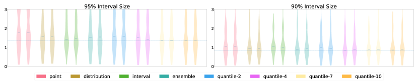
Figure 2: Comparing the interval size from conformal interval prediction (left of each pair) versus credible intervals from recalibrated predictors (right of each pair) for a variety of base prediction types.The intervals from both methods obtain the nominal coverage. The distribution of interval sizes are very similar between the two methods, indicating that recalibration is empirically comparable to conformal interval prediction in its ability to provide interval predictions.

On the choice of base predictor

We find that all base prediction types can be recalibrated to give models with very good calibration. All base predictors we tested achieved an average test ECE of less than 0.007 after recalibration, across the 17 datasets. This is consistent with the calibration guarantee given by our framework, which says that a recalibrated model will be $O(1/n)$-calibrated.

Quantile predictors performed best on the other four metrics we considered: quantile-10 performed best on the two sharpness metrics STD and 95% CI Width, while quantile-4 performed best in terms of NLL and the three quantile predictors had the same performance on CRPS (see Table 3). Interestingly, quantile base predictors outperformed distribution estimators on NLL, even though the distribution predictors were directly trained to optimize NLL. These results indicate that quantile prediction is a promising strategy for learning distribution predictors.

On the choice of calibration score

We investigate the role of the calibration score for a base predictor that already makes distribution predictions (see Table 2). Specifically, we compare two natural choices: $\varphi_{\text{cdf}}$ and $\varphi_{\text{zscore}}$. The $\varphi_{\text{cdf}}$ calibration score computes the quantile of the observed label under the predicted distribution, and is the calibration score used by isotonic calibration and conformal calibration. The $\varphi_{\text{cdf}}$ calibration score computes the number of standard deviations between the mean of the predicted distribution and the observed label. We find that $\varphi_{\text{z-score}}$ and $\varphi_{\text{cdf}}$ are effective under different metrics. The $\varphi_{\text{cdf}}$ calibration score performs better for CRPS and 95% CI Width, while $\varphi_{\text{zscore}}$ performs better for NLL and STD.

On the choice of interpolation algorithm

We compare three interpolation algorithms: Linear interpolation which is simple and stable, random interpolation which provides improved calibration guarantees, and Neural Autoregressive Flow (NAF) interpolation which uses a more sophisticated neural network approach to interpolation. We find that NAF interpolation performs best on NLL and 95% CI Width, linear interpolation performs best on STD, and random interpolation performs best on CRPS. The random interpolator leads to distribution predictions with infinite STD and undefine NLL, so is not appropriate when those metrics are of importance. The most appropriate interpolator is likely to vary between use cases.

On interval prediction

In this experiment, we explore whether recalibration can yield high quality interval predictions, by comparing to conformal interval prediction, a standard approach for producing interval predictors from any base predictor. Recall that Theorem 2 tells us that conformal interval prediction can approximately be recovered by taking some credible interval of a recalibrated predictor. However, since we cannot identify which credible interval it should be a priori, we test in these experiments whether it is sufficient to simply take the centered credible interval; for example, the interval between the 5% and 95% quantiles of the predicted distributions.

We find that this recalibration yields interval predictions that effectively approximate conformal interval prediction (see Figure 2). Conformal interval prediction tends to produce slightly shorter intervals than recalibration (both methods achieve the nominal coverage). This shows that recalibration can be applied broadly, even when the downstream task is unknown. If we recalibrate a model to make distribution predictions then decide that we need interval predictions, we can extract credible intervals from the distribution predictor that are comparable to methods designed to directly produce interval predictions.

7 Discussion

Recalibration is a convenient and effective way to build calibrated distribution predictors. Flexible methods for uncertainty quantification empower more practitioners to use uncertainty quantification, improving the reliability of both fully-automated systems and decision support systems. Modular conformal calibration organizes and simplifies the process of choosing a recalibration technique, and provides guarantees that the resulting models will be calibrated. As a consequence, we believe that further developing principled and adaptive techniques for choosing between these recalibration algorithms is a promising direction for future work.

Appendix A Interpolation Algorithms

Quantile Prediction

Recall that the interpretation of a quantile prediction is that the probability $y$ is less than $f_{k}(x)$ should be $\alpha_{k}$, for $k=1,\dots,K$.

$$\varphi_{\text{quantile}}(x,y)=\left\{\begin{array}[]{ll}\alpha_{K}+y-f_{K}(x)&y>f_{K}(x)\\ \alpha_{k}+\frac{y-f_{k}(x)}{f_{k+1}(x)-f_{k}(x)}(\alpha_{k+1}-\alpha_{k})&f_{k}(x)<y\leq f_{k+1}(x),\text{for }k=1,\cdots,K-1\\ \alpha_{1}+y-f_{1}(x)&y\leq f_{1}(x)\\ \end{array}\right.$$

Intuitively, if $y$ exactly equals the $\alpha_{k}$-th quantile, then $\varphi_{0}(x,y)=\alpha_{k}$. For other values we use a linear interpolation.

Ensemble Prediction

Given an ensemble consisting of $K$ predictors, we can define the calibration score recursively: for each of the $M$ predictors in the ensemble, we choose a calibration score $\varphi_{m}$; the overall calibration score $\varphi_{\text{ensemble}}$ is the summed calibration score $\varphi_{\text{ensemble}}(x,y)=\sum_{k}\varphi_{k}(x,y)$. Naturally, if there is prior information about the quality of these predictions, we can use a weighted sum where the higher quality predictions are given a higher weight.

Appendix B Proper Non-conformity Score

To ensure that conformal prediction algorithms are “well-behaved”, it is typical to put some restrictions on the non-conformity score. In particular, we say that a non-conformity score is proper if it is continuous and strictly unimodal in $y$. We require strict unimodality and continuity to ensure that the confidence intervals change smoothly when $c$ increases or decreases. Intuitively, an infinitesimal increase in $c$ should lead to an infinitesimal increase in the confidence interval.

Appendix C Proofs

The important property of conformal prediction is that it is always $1/n$-exact (as in Definition 2), regardless of the true distribution of $X,Y$ and the non-conformity score $\phi$.

Proposition 1.

For any non-conformity score $\phi$, if $\phi(X,Y)$ is absolutely continuous, then the conformal interval predictor $I_{c}$ is $1/n$-exact.

Proof of Proposition 1 .

$$\Pr[Y\in I_{c}(X)]=\Pr\left[\frac{1}{n}\#\{i\mid\phi(X_{i},Y_{i})\leq\phi(X,y)\}\leq c\right]$$

$$={\mathbb{E}}\left[\Pr\left[\frac{1}{n}\#\{i\mid\phi(X_{i},Y_{i})\leq\phi(X,Y)\}\leq c\mid\lbag Z_{1},\cdots,Z_{n},(X,Y)\rbag\right]\right]$$

$$=\frac{\lfloor nc\rfloor}{n}>\frac{nc-1}{n}=c-\frac{1}{n}$$

where $Z_{i}=(X_{i},Y_{i})$. ∎

See 1

Proof of Theorem 1.

By our assumption of absolute continuity, almost surely we have $a^{\prime}_{1}\neq a^{\prime}_{2}\neq\cdots\neq a^{\prime}_{T}\neq\varphi(X^{*},Y)$. For notation convenience we also let $a_{t}=-\infty$ if $t<1$ and $a_{t}=+\infty$ if $t>T$.

By the assumption $\frac{t-\ lambda}{T+1}<q(a^{\prime}_{t})<\frac{t+\lambda}{T+1}$, if $q(a)\geq\frac{t+\lambda}{T+1}$ then $q(a)>q(a_{t}^{\prime})$, which by monotonicity implies that $a>a_{t}^{\prime}$, i.e.

$$\text{if }q(a)\geq\frac{t+\lambda}{T+1}\text{ then }a>a_{t}^{\prime}$$ (9)

similarly

$$\text{if }q(a)\leq\frac{t-\lambda}{T+1}\text{ then }a<a_{t}^{\prime}$$ (10)

$$\Pr[H[X^{*}](Y)\leq c]:=\Pr[q(\varphi(X^{*},Y))\leq c]$$ Definition

$$\leq\Pr\left[q(\varphi(X^{*},Y))\leq\frac{\lceil cT+c+\lambda\rceil-\lambda}{T+1}\right] [i]$$

$$\leq\Pr\left[\varphi(X^{*},Y)<a_{\lceil cT+c+\lambda\rceil}^{\prime}\right] [i]+\text{Eq.(\ref{eq:implication2})}$$

$$={\mathbb{E}}\left[\Pr\left[\varphi(X^{*},Y)<a_{\lceil cT+c+\lambda\rceil}^{\prime}\mid\lbag Z_{1},\cdots,Z_{T},(X^{*},Y)\rbag\right]\right]$$ Tower

$$\leq\lceil cT+c+\lambda\rceil/(T+1)$$ Symmetry

Where explanation $[i]$ is based on the property ”$A\implies B\text{ then }\Pr[A]\leq\Pr[B]$”; the last inequality is usually an equality except when $c\approx 1$ then the upper bound will be greater than $1$. Similarly we have

$$\Pr[H[X_{*}](Y)\leq c]:=1-\Pr[q(\varphi(X^{*},Y))>c]$$ Definition

$$\geq 1-\Pr\left[q(\varphi(X^{*},Y))\geq\frac{\lfloor cT+c-\lambda\rfloor+\lambda}{T+1}\right] [i]$$

$$\geq 1-\Pr\left[\varphi(X^{*},Y)>a_{\lfloor cT+c-\lambda\rfloor}^{\prime}\right] [i]+\text{Eq.(\ref{eq:implication1})}$$

$$=1-{\mathbb{E}}\left[\Pr\left[\varphi(X^{*},Y)>a_{\lfloor cT+c-\lambda\rfloor}^{\prime}\mid\lbag Z_{1},\cdots,Z_{T},(X^{*},Y)\rbag\right]\right]$$ Tower

$$={\mathbb{E}}\left[1-\Pr\left[\varphi(X^{*},Y)>a_{\lfloor cT+c-\lambda\rfloor}^{\prime}\mid\lbag Z_{1},\cdots,Z_{T},(X^{*},Y)\rbag\right]\right]$$ Linear

$$={\mathbb{E}}\left[\Pr\left[\varphi(X^{*},Y)\leq a_{\lfloor cT+c-\lambda\rfloor}^{\prime}\mid\lbag Z_{1},\cdots,Z_{T},(X^{*},Y)\rbag\right]\right]$$ Linear

$$\geq\lfloor cT+c-\lambda\rfloor/(T+1)$$ Symmetry

Therefore we have

$$\Pr[H[X_{*}](Y)\leq c]-c \leq\frac{\lceil cT+c+\lambda\rceil}{T+1}-c<\frac{cT+c+\lambda+1}{T+1}-c=\frac{1+\lambda}{T+1}$$

$$\Pr[H[X_{*}](Y)\leq c]-c \geq\frac{\lfloor cT+c-\lambda\rfloor}{T+1}-c>\frac{cT+c-\lambda-1}{T+1}-c=\frac{-1-\lambda}{T+1}$$

So combined we have (for any $c\in(0,1)$)

$$\left\lvert\Pr[H[X_{*}](Y)\leq c]-c\right\rvert\leq\frac{1+\lambda}{T+1}$$

∎

See 2

]

Figure 4: Illustration of the proof of Theorem 2

Proof of Theorem 2.

We will use a constructive proof. Because conformal prediction algorithm does not change if we add a constant to the non-conformity score, so without loss of generality, assume $0$ is a lower bound on $\phi$. Denote $y_{\mathrm{min}}(\phi;x)$ as a global minimizer of $\phi(x,\cdot)$, i.e.

$$\phi(x,y_{\mathrm{min}}(\phi;x))\leq\phi(x,y),\forall y\in{\mathcal{Y}}$$ (11)

Define

$$\varphi(x,y)=\left\{\begin{array}[]{ll}-\phi(x,y)&y\leq y_{\mathrm{min}}(\phi;x)\\ \phi(x,y)&y>y_{\mathrm{min}}(\phi;x)\end{array}\right.$$

Based on this construction we have $\phi(x,y)=|\varphi(x,y)|$. In addition because $\phi$ is uni-modal, $\varphi$ is monotonically non-decreasing, so $\varphi$ satisfies the condition as a calibration score. As a notation convenience we will also denote $\varphi(x,y)=\varphi_{x}(y)$.

Consider the conformal interval predictor (for notation convenience we will drop its dependence on $Z_{1},\cdots,Z_{T},X^{*}$)

$${\Gamma_{\mathrm{interval}}}:=(L,U) =\left\{y\mid\frac{1}{T}\#\{t\mid|\varphi_{X_{t}}(Y_{t})|\leq|\varphi_{X^{*}}(y)|\}\leq c\right\}$$

First of all, observe that because $A$ is continuous, we must $|\varphi_{X^{*}}(U)|=|\varphi_{X^{*}}(L)|$. This intuition is illustrated in Figure 4. Therefore

$$\{\#t\mid|\varphi_{X_{t}}(Y_{t})|\leq|\varphi_{X^{*}}(L)|\} =\{\#t\mid|\varphi_{X_{t}}(Y_{t})|\leq|\varphi_{X^{*}}(U)|\}$$

$$=\{\#t\mid\varphi_{X^{*}}(L)\leq\varphi_{X_{t}}(Y_{t})\leq\varphi_{X^{*}}(U)\}$$

Second we wish to prove that

$$cT\leq\#\{t\mid|\varphi_{X_{t}}(Y_{t})|\leq|\varphi_{X^{*}}(U)|\}\leq cT+1$$

This is because if $\#\{t\mid|\varphi_{X_{t}}(Y_{t})|\leq|\varphi_{X^{*}}(U)|\}<cT$ then because of continuity of $\phi$, almost surely choosing $U^{\prime}=U+\kappa$ for sufficiently small $\kappa>0$ still satisfies $\#\{t\mid|\varphi_{X_{t}}(Y_{t})|\leq|\varphi_{X^{*}}(U^{\prime})|\}<cT$, therefore $U^{\prime}\in(L,U)$ but $U^{\prime}>U$, which is a contradiction.

If on the other hand, $\#\{t\mid|\varphi_{X_{t}}(Y_{t})|\leq|\varphi_{X^{*}}(U)|\}>cT+1$, then let $U^{\prime}=U-\kappa$ for sufficiently small $\kappa>0$ we have $\#\{t\mid|\varphi_{X_{t}}(Y_{t})|\leq|\varphi_{X^{*}}(U)|\}>cT$. This means that $U^{\prime}\not\in(L,U)$ but $U^{\prime}<U$, which is a contradiction.

We observe that there are two possibilities, these two situations are illustrated in Figure 4: situation 1. there exists a $t$ such that $\varphi_{X_{t}}(Y_{t})=\varphi_{X^{*}}(U)$; situation 2. there exists a $t$ such that $\varphi_{X_{t}}(Y_{t})=\varphi_{X^{*}}(L)$.

We first consider situation 1. Denote $D=\#\{t,\varphi_{X^{*}}(L)<\varphi_{X_{t}}(Y_{t})\leq\varphi_{X^{*}}(U)\}$ and $B=\#\{t,\varphi_{X_{t}}(Y_{t})\leq\varphi_{X^{*}}(L)\}$. We know that $cT\leq D<cT+1$. Then by the assumption that the interpolation algorithm is $0$-exact we have

$$H[X_{*}](U)=\frac{D+B+1}{T+1},H[X](L)\in\left[\frac{B+1}{T+1},\frac{B+2}{T+1}\right)$$

So their difference is bounded by

$$\frac{D-1}{T+1} <H[X_{*}](U)-H[X_{*}](L)\leq\frac{D}{T+1}$$ (12)

$$\frac{cT-1}{T+1} <H[X_{*}](U)-H[X_{*}](L)<\frac{cT+1}{T+1}$$

Therefore

$$H[X_{*}](U)-H[X_{*}](L)-c \leq\frac{cT+1}{T+1}-c=\frac{1-c}{T+1}$$

$$c-H[X_{*}](U)-H[X_{*}](L) \geq c-\frac{cT-1}{T+1}=\frac{c-1}{T+1}$$

Combined we have

$$H[X](U)-H[X](L)\in c\pm\frac{|1-c|}{T+1}$$

Now we consider situation 2. Denote $D^{\prime}=\#\{t,\varphi_{X^{*}}(L)\leq\varphi_{X_{t}}(Y_{t})<\varphi_{X^{*}}(U)\}$ and $B^{\prime}=\#\{t,\varphi_{X_{t}}(Y_{t})<\varphi_{X^{*}}(L)\}$. Again we know that $cT\leq D^{\prime}<cT+1$. Then by the assumption that the interpolation algorithm is $0$-exact we have

$$H[X_{*}](U)\in\left[\frac{D^{\prime}+B^{\prime}+1}{T+1},\frac{D^{\prime}+B^{\prime}+2}{T+1}\right),H[X_{*}](L)=\frac{B^{\prime}+2}{T+1}$$

So their difference is bounded by

$$\frac{D^{\prime}-1}{T+1} <H[X_{*}](U)-H[X_{*}](L)\leq\frac{D^{\prime}}{T+1}$$ (13)

This is identical to Eq.(12) so the rest of the proof will follow identically. ∎

Appendix D Additional Experimental Results

		STD	95% CI Width	NLL	CRPS	ECE
blog	zscore-NAF	$\cellcolor{green!25}{\mathbf{0.553\pm 0.006}}$	$2.737\pm 0.151$	$0.178\pm 0.039$	$\cellcolor{green!25}{\mathbf{0.287\pm 0.003}}$	$0.002\pm 0.001$
	cdf-linear	$1.380\pm 0.513$	$3.074\pm 0.475$	$\cellcolor{green!25}{\mathbf{0.064\pm 0.062}}$	$0.289\pm 0.002$	$\cellcolor{green!25}{\mathbf{0.001\pm 0.001}}$
	cdf-NAF	$0.592\pm 0.061$	$\cellcolor{green!25}{\mathbf{2.027\pm 0.201}}$	$0.944\pm 1.229$	$0.328\pm 0.049$	$0.039\pm 0.028$
	zscore-random	$0.567\pm 0.007$	$2.657\pm 0.101$	$4.087\pm 0.102$	$0.288\pm 0.003$	$0.002\pm 0.001$
	cdf-random	$1.381\pm 0.513$	$3.074\pm 0.475$	$4.069\pm 0.096$	$0.289\pm 0.002$	$\cellcolor{green!25}{\mathbf{0.001\pm 0.001}}$
	zscore-linear	$0.567\pm 0.007$	$2.657\pm 0.101$	$0.321\pm 0.040$	$0.288\pm 0.003$	$0.002\pm 0.001$
boston	zscore-NAF	$0.337\pm 0.019$	$1.589\pm 0.195$	$0.467\pm 0.117$	$\cellcolor{green!25}{\mathbf{0.173\pm 0.012}}$	$\cellcolor{green!25}{\mathbf{0.009\pm 0.010}}$
	cdf-linear	$0.372\pm 0.031$	$1.527\pm 0.118$	$0.642\pm 0.075$	$\cellcolor{green!25}{\mathbf{0.173\pm 0.012}}$	$\cellcolor{green!25}{\mathbf{0.009\pm 0.009}}$
	cdf-NAF	$0.357\pm 0.025$	$1.539\pm 0.124$	$\cellcolor{green!25}{\mathbf{0.363\pm 0.070}}$	$0.174\pm 0.012$	$\cellcolor{green!25}{\mathbf{0.009\pm 0.010}}$
	zscore-random	$0.335\pm 0.018$	$1.520\pm 0.121$	$13.622\pm 0.094$	$\cellcolor{green!25}{\mathbf{0.173\pm 0.012}}$	$\cellcolor{green!25}{\mathbf{0.009\pm 0.009}}$
	cdf-random	N/A	$1.532\pm 0.121$	$13.588\pm 0.114$	N/A	$\cellcolor{green!25}{\mathbf{0.009\pm 0.009}}$
	zscore-linear	$\cellcolor{green!25}{\mathbf{0.331\pm 0.017}}$	$\cellcolor{green!25}{\mathbf{1.449\pm 0.111}}$	$0.674\pm 0.068$	$\cellcolor{green!25}{\mathbf{0.173\pm 0.012}}$	$\cellcolor{green!25}{\mathbf{0.009\pm 0.009}}$
concrete	zscore-NAF	$0.325\pm 0.017$	$1.402\pm 0.186$	$0.325\pm 0.066$	$\cellcolor{green!25}{\mathbf{0.163\pm 0.007}}$	$\cellcolor{green!25}{\mathbf{0.005\pm 0.005}}$
	cdf-linear	$0.317\pm 0.016$	$1.287\pm 0.086$	$0.576\pm 0.054$	$\cellcolor{green!25}{\mathbf{0.163\pm 0.007}}$	$\cellcolor{green!25}{\mathbf{0.005\pm 0.005}}$
	cdf-NAF	$0.312\pm 0.016$	$1.354\pm 0.078$	$\cellcolor{green!25}{\mathbf{0.251\pm 0.051}}$	$\cellcolor{green!25}{\mathbf{0.163\pm 0.007}}$	$\cellcolor{green!25}{\mathbf{0.005\pm 0.006}}$
	zscore-random	$0.310\pm 0.014$	$1.287\pm 0.087$	$13.206\pm 0.090$	$\cellcolor{green!25}{\mathbf{0.163\pm 0.007}}$	$\cellcolor{green!25}{\mathbf{0.005\pm 0.005}}$
	cdf-random	N/A	$1.288\pm 0.086$	$13.212\pm 0.100$	N/A	$\cellcolor{green!25}{\mathbf{0.005\pm 0.005}}$
	zscore-linear	$\cellcolor{green!25}{\mathbf{0.309\pm 0.014}}$	$\cellcolor{green!25}{\mathbf{1.279\pm 0.084}}$	$0.593\pm 0.057$	$\cellcolor{green!25}{\mathbf{0.163\pm 0.007}}$	$\cellcolor{green!25}{\mathbf{0.005\pm 0.005}}$
crime	zscore-NAF	$0.498\pm 0.013$	$2.062\pm 0.084$	$1.764\pm 0.123$	$0.309\pm 0.008$	$0.010\pm 0.006$
	cdf-linear	$0.644\pm 0.029$	$2.406\pm 0.066$	$1.077\pm 0.057$	$\cellcolor{green!25}{\mathbf{0.308\pm 0.007}}$	$\cellcolor{green!25}{\mathbf{0.006\pm 0.006}}$
	cdf-NAF	$0.570\pm 0.014$	$2.161\pm 0.053$	$\cellcolor{green!25}{\mathbf{0.814\pm 0.067}}$	$0.311\pm 0.007$	$\cellcolor{green!25}{\mathbf{0.006\pm 0.006}}$
	zscore-random	$\cellcolor{green!25}{\mathbf{0.487\pm 0.011}}$	$\cellcolor{green!25}{\mathbf{1.900\pm 0.036}}$	$13.308\pm 0.071$	$\cellcolor{green!25}{\mathbf{0.308\pm 0.008}}$	$\cellcolor{green!25}{\mathbf{0.006\pm 0.006}}$
	cdf-random	N/A	$2.406\pm 0.066$	$13.274\pm 0.054$	N/A	$\cellcolor{green!25}{\mathbf{0.006\pm 0.006}}$
	zscore-linear	$\cellcolor{green!25}{\mathbf{0.487\pm 0.011}}$	$\cellcolor{green!25}{\mathbf{1.900\pm 0.036}}$	$1.901\pm 0.130$	$\cellcolor{green!25}{\mathbf{0.308\pm 0.008}}$	$\cellcolor{green!25}{\mathbf{0.006\pm 0.006}}$
energy	zscore-NAF	$0.174\pm 0.013$	$\cellcolor{green!25}{\mathbf{0.652\pm 0.043}}$	$\cellcolor{green!25}{\mathbf{-0.394\pm 0.097}}$	$\cellcolor{green!25}{\mathbf{0.099\pm 0.008}}$	$\cellcolor{green!25}{\mathbf{0.010\pm 0.006}}$
-efficiency	cdf-linear	$\cellcolor{green!25}{\mathbf{0.168\pm 0.010}}$	$0.668\pm 0.040$	$0.027\pm 0.108$	$\cellcolor{green!25}{\mathbf{0.099\pm 0.008}}$	$\cellcolor{green!25}{\mathbf{0.010\pm 0.006}}$
	cdf-NAF	$\cellcolor{green!25}{\mathbf{0.168\pm 0.010}}$	$0.681\pm 0.039$	$-0.342\pm 0.101$	$\cellcolor{green!25}{\mathbf{0.099\pm 0.008}}$	$\cellcolor{green!25}{\mathbf{0.010\pm 0.006}}$
	zscore-random	$0.180\pm 0.010$	$0.667\pm 0.040$	$13.253\pm 0.130$	$\cellcolor{green!25}{\mathbf{0.099\pm 0.008}}$	$\cellcolor{green!25}{\mathbf{0.010\pm 0.006}}$
	cdf-random	N/A	$0.668\pm 0.040$	$13.252\pm 0.125$	N/A	$\cellcolor{green!25}{\mathbf{0.010\pm 0.006}}$
	zscore-linear	$0.172\pm 0.011$	$0.666\pm 0.040$	$0.003\pm 0.107$	$\cellcolor{green!25}{\mathbf{0.099\pm 0.008}}$	$\cellcolor{green!25}{\mathbf{0.010\pm 0.006}}$
fb-comment1	zscore-NAF	$0.376\pm 0.009$	$1.459\pm 0.028$	$\cellcolor{green!25}{\mathbf{0.066\pm 0.015}}$	$\cellcolor{green!25}{\mathbf{0.210\pm 0.001}}$	$\cellcolor{green!25}{\mathbf{0.002\pm 0.001}}$
	cdf-linear	$0.880\pm 0.119$	$1.692\pm 0.034$	$0.120\pm 0.017$	$\cellcolor{green!25}{\mathbf{0.210\pm 0.001}}$	$\cellcolor{green!25}{\mathbf{0.002\pm 0.001}}$
	cdf-NAF	$\cellcolor{green!25}{\mathbf{0.344\pm 0.054}}$	$\cellcolor{green!25}{\mathbf{1.156\pm 0.195}}$	$2.841\pm 2.106$	$0.288\pm 0.075$	$0.091\pm 0.046$
	zscore-random	$0.397\pm 0.004$	$1.692\pm 0.034$	$5.196\pm 0.030$	$\cellcolor{green!25}{\mathbf{0.210\pm 0.001}}$	$\cellcolor{green!25}{\mathbf{0.002\pm 0.001}}$
	cdf-random	$0.880\pm 0.119$	$1.692\pm 0.034$	$5.220\pm 0.029$	$\cellcolor{green!25}{\mathbf{0.210\pm 0.001}}$	$\cellcolor{green!25}{\mathbf{0.002\pm 0.001}}$
	zscore-linear	$0.397\pm 0.004$	$1.692\pm 0.034$	$0.261\pm 0.015$	$\cellcolor{green!25}{\mathbf{0.210\pm 0.001}}$	$\cellcolor{green!25}{\mathbf{0.002\pm 0.001}}$
fb-comment2	zscore-NAF	$0.368\pm 0.010$	$1.423\pm 0.021$	$\cellcolor{green!25}{\mathbf{0.053\pm 0.025}}$	$\cellcolor{green!25}{\mathbf{0.207\pm 0.002}}$	$\cellcolor{green!25}{\mathbf{0.001\pm 0.001}}$
	cdf-linear	$0.459\pm 0.017$	$1.573\pm 0.016$	$0.118\pm 0.027$	$\cellcolor{green!25}{\mathbf{0.207\pm 0.002}}$	$\cellcolor{green!25}{\mathbf{0.001\pm 0.001}}$
	cdf-NAF	$\cellcolor{green!25}{\mathbf{0.347\pm 0.035}}$	$\cellcolor{green!25}{\mathbf{1.294\pm 0.171}}$	N/A	$0.273\pm 0.083$	N/A
	zscore-random	$0.386\pm 0.004$	$1.573\pm 0.016$	$3.739\pm 0.031$	$\cellcolor{green!25}{\mathbf{0.207\pm 0.002}}$	$\cellcolor{green!25}{\mathbf{0.001\pm 0.001}}$
	cdf-random	$0.459\pm 0.017$	$1.573\pm 0.016$	$3.731\pm 0.037$	$\cellcolor{green!25}{\mathbf{0.207\pm 0.002}}$	$\cellcolor{green!25}{\mathbf{0.001\pm 0.001}}$
	zscore-linear	$0.386\pm 0.004$	$1.573\pm 0.016$	$0.194\pm 0.023$	$\cellcolor{green!25}{\mathbf{0.207\pm 0.002}}$	$\cellcolor{green!25}{\mathbf{0.001\pm 0.001}}$
forest-fires	zscore-NAF	$1.167\pm 0.043$	$4.697\pm 0.214$	$1.959\pm 0.137$	$\cellcolor{green!25}{\mathbf{0.601\pm 0.023}}$	$0.018\pm 0.008$
	cdf-linear	$1.285\pm 0.162$	$4.874\pm 0.380$	$1.964\pm 0.086$	$\cellcolor{green!25}{\mathbf{0.601\pm 0.022}}$	$\cellcolor{green!25}{\mathbf{0.017\pm 0.008}}$
	cdf-NAF	$1.219\pm 0.078$	$4.801\pm 0.339$	$\cellcolor{green!25}{\mathbf{1.637\pm 0.087}}$	$0.607\pm 0.023$	$\cellcolor{green!25}{\mathbf{0.017\pm 0.008}}$
	zscore-random	$1.156\pm 0.041$	$4.529\pm 0.185$	$13.648\pm 0.102$	$\cellcolor{green!25}{\mathbf{0.601\pm 0.023}}$	$\cellcolor{green!25}{\mathbf{0.017\pm 0.008}}$
	cdf-random	N/A	$4.862\pm 0.381$	$13.659\pm 0.099$	N/A	$\cellcolor{green!25}{\mathbf{0.017\pm 0.008}}$
	zscore-linear	$\cellcolor{green!25}{\mathbf{1.147\pm 0.043}}$	$\cellcolor{green!25}{\mathbf{4.455\pm 0.219}}$	$2.121\pm 0.124$	$\cellcolor{green!25}{\mathbf{0.601\pm 0.023}}$	$\cellcolor{green!25}{\mathbf{0.017\pm 0.008}}$
kin8nm	zscore-NAF	$0.300\pm 0.006$	$\cellcolor{green!25}{\mathbf{1.107\pm 0.016}}$	$0.127\pm 0.012$	$\cellcolor{green!25}{\mathbf{0.152\pm 0.002}}$	$\cellcolor{green!25}{\mathbf{0.003\pm 0.002}}$
	cdf-linear	$\cellcolor{green!25}{\mathbf{0.281\pm 0.003}}$	$1.121\pm 0.013$	$0.490\pm 0.015$	$\cellcolor{green!25}{\mathbf{0.152\pm 0.002}}$	$\cellcolor{green!25}{\mathbf{0.003\pm 0.002}}$
	cdf-NAF	$\cellcolor{green!25}{\mathbf{0.281\pm 0.003}}$	$1.149\pm 0.015$	$\cellcolor{green!25}{\mathbf{0.112\pm 0.014}}$	$\cellcolor{green!25}{\mathbf{0.152\pm 0.002}}$	$\cellcolor{green!25}{\mathbf{0.003\pm 0.002}}$
	zscore-random	$\cellcolor{green!25}{\mathbf{0.281\pm 0.003}}$	$1.121\pm 0.013$	$11.279\pm 0.090$	$\cellcolor{green!25}{\mathbf{0.152\pm 0.002}}$	$\cellcolor{green!25}{\mathbf{0.003\pm 0.002}}$
	cdf-random	$\cellcolor{green!25}{\mathbf{0.281\pm 0.003}}$	$1.121\pm 0.013$	$11.291\pm 0.073$	$\cellcolor{green!25}{\mathbf{0.152\pm 0.002}}$	$\cellcolor{green!25}{\mathbf{0.003\pm 0.002}}$
	zscore-linear	$\cellcolor{green!25}{\mathbf{0.281\pm 0.003}}$	$1.121\pm 0.013$	$0.486\pm 0.014$	$\cellcolor{green!25}{\mathbf{0.152\pm 0.002}}$	$\cellcolor{green!25}{\mathbf{0.003\pm 0.002}}$

Table 4: Experimental results for individual datasets.

		STD	95% CI Width	NLL	CRPS	ECE
medical	zscore-NAF	$0.935\pm 0.008$	$4.465\pm 0.064$	$1.548\pm 0.015$	$0.463\pm 0.002$	$0.003\pm 0.001$
-expenditure	cdf-linear	$0.963\pm 0.009$	$3.648\pm 0.037$	$1.643\pm 0.009$	$\cellcolor{green!25}{\mathbf{0.462\pm 0.002}}$	$\cellcolor{green!25}{\mathbf{0.002\pm 0.001}}$
	cdf-NAF	$0.928\pm 0.010$	$\cellcolor{green!25}{\mathbf{3.616\pm 0.110}}$	$\cellcolor{green!25}{\mathbf{1.381\pm 0.057}}$	$0.465\pm 0.002$	$0.005\pm 0.004$
	zscore-random	$\cellcolor{green!25}{\mathbf{0.893\pm 0.004}}$	$3.648\pm 0.037$	$10.869\pm 0.041$	$\cellcolor{green!25}{\mathbf{0.462\pm 0.002}}$	$\cellcolor{green!25}{\mathbf{0.002\pm 0.001}}$
	cdf-random	$0.963\pm 0.009$	$3.648\pm 0.037$	$10.866\pm 0.034$	$\cellcolor{green!25}{\mathbf{0.462\pm 0.002}}$	$\cellcolor{green!25}{\mathbf{0.002\pm 0.001}}$
	zscore-linear	$\cellcolor{green!25}{\mathbf{0.893\pm 0.004}}$	$3.648\pm 0.037$	$1.818\pm 0.015$	$\cellcolor{green!25}{\mathbf{0.462\pm 0.002}}$	$\cellcolor{green!25}{\mathbf{0.002\pm 0.001}}$
mpg	zscore-NAF	$0.396\pm 0.021$	$1.832\pm 0.186$	$0.555\pm 0.114$	$\cellcolor{green!25}{\mathbf{0.186\pm 0.011}}$	$\cellcolor{green!25}{\mathbf{0.019\pm 0.013}}$
	cdf-linear	$0.392\pm 0.030$	$1.554\pm 0.110$	$0.821\pm 0.099$	$\cellcolor{green!25}{\mathbf{0.186\pm 0.011}}$	$0.020\pm 0.013$
	cdf-NAF	$0.383\pm 0.026$	$1.652\pm 0.138$	$\cellcolor{green!25}{\mathbf{0.551\pm 0.084}}$	$0.187\pm 0.011$	$\cellcolor{green!25}{\mathbf{0.019\pm 0.013}}$
	zscore-random	$0.380\pm 0.018$	$1.545\pm 0.109$	$13.696\pm 0.073$	$\cellcolor{green!25}{\mathbf{0.186\pm 0.011}}$	$0.020\pm 0.013$
	cdf-random	N/A	$1.546\pm 0.110$	$13.651\pm 0.092$	N/A	$0.020\pm 0.013$
	zscore-linear	$\cellcolor{green!25}{\mathbf{0.377\pm 0.018}}$	$\cellcolor{green!25}{\mathbf{1.538\pm 0.108}}$	$0.756\pm 0.096$	$\cellcolor{green!25}{\mathbf{0.186\pm 0.011}}$	$\cellcolor{green!25}{\mathbf{0.019\pm 0.013}}$
naval	zscore-NAF	$\cellcolor{green!25}{\mathbf{0.041\pm 0.002}}$	$0.165\pm 0.008$	$-1.904\pm 0.036$	$\cellcolor{green!25}{\mathbf{0.025\pm 0.001}}$	$\cellcolor{green!25}{\mathbf{0.002\pm 0.001}}$
	cdf-linear	$0.042\pm 0.002$	$\cellcolor{green!25}{\mathbf{0.162\pm 0.007}}$	$-1.716\pm 0.029$	$\cellcolor{green!25}{\mathbf{0.025\pm 0.001}}$	$\cellcolor{green!25}{\mathbf{0.002\pm 0.001}}$
	cdf-NAF	$0.042\pm 0.002$	$0.173\pm 0.008$	$\cellcolor{green!25}{\mathbf{-1.915\pm 0.027}}$	$\cellcolor{green!25}{\mathbf{0.025\pm 0.001}}$	$\cellcolor{green!25}{\mathbf{0.002\pm 0.001}}$
	zscore-random	$0.042\pm 0.002$	$\cellcolor{green!25}{\mathbf{0.162\pm 0.007}}$	$1.355\pm 0.125$	$\cellcolor{green!25}{\mathbf{0.025\pm 0.001}}$	$\cellcolor{green!25}{\mathbf{0.002\pm 0.001}}$
	cdf-random	$0.042\pm 0.002$	$\cellcolor{green!25}{\mathbf{0.162\pm 0.007}}$	$1.330\pm 0.114$	$\cellcolor{green!25}{\mathbf{0.025\pm 0.001}}$	$\cellcolor{green!25}{\mathbf{0.002\pm 0.001}}$
	zscore-linear	$0.042\pm 0.002$	$\cellcolor{green!25}{\mathbf{0.162\pm 0.007}}$	$-1.717\pm 0.029$	$\cellcolor{green!25}{\mathbf{0.025\pm 0.001}}$	$\cellcolor{green!25}{\mathbf{0.002\pm 0.001}}$
power-plant	zscore-NAF	$\cellcolor{green!25}{\mathbf{0.218\pm 0.003}}$	$\cellcolor{green!25}{\mathbf{0.845\pm 0.007}}$	$\cellcolor{green!25}{\mathbf{-0.104\pm 0.010}}$	$\cellcolor{green!25}{\mathbf{0.120\pm 0.001}}$	$\cellcolor{green!25}{\mathbf{0.003\pm 0.002}}$
	cdf-linear	$0.225\pm 0.003$	$0.854\pm 0.009$	$0.244\pm 0.011$	$\cellcolor{green!25}{\mathbf{0.120\pm 0.001}}$	$\cellcolor{green!25}{\mathbf{0.003\pm 0.002}}$
	cdf-NAF	$0.224\pm 0.003$	$0.886\pm 0.011$	$-0.101\pm 0.010$	$0.121\pm 0.001$	$\cellcolor{green!25}{\mathbf{0.003\pm 0.002}}$
	zscore-random	$0.219\pm 0.002$	$0.854\pm 0.009$	$10.208\pm 0.074$	$\cellcolor{green!25}{\mathbf{0.120\pm 0.001}}$	$\cellcolor{green!25}{\mathbf{0.003\pm 0.002}}$
	cdf-random	$0.225\pm 0.003$	$0.854\pm 0.009$	$10.208\pm 0.067$	$\cellcolor{green!25}{\mathbf{0.120\pm 0.001}}$	$\cellcolor{green!25}{\mathbf{0.003\pm 0.002}}$
	zscore-linear	$\cellcolor{green!25}{\mathbf{0.218\pm 0.002}}$	$0.854\pm 0.009$	$0.251\pm 0.011$	$\cellcolor{green!25}{\mathbf{0.120\pm 0.001}}$	$\cellcolor{green!25}{\mathbf{0.003\pm 0.002}}$
protein	zscore-NAF	$0.622\pm 0.011$	$2.246\pm 0.027$	$\cellcolor{green!25}{\mathbf{0.765\pm 0.019}}$	$\cellcolor{green!25}{\mathbf{0.339\pm 0.003}}$	$\cellcolor{green!25}{\mathbf{0.001\pm 0.001}}$
	cdf-linear	$0.709\pm 0.020$	$2.333\pm 0.024$	$0.960\pm 0.018$	$\cellcolor{green!25}{\mathbf{0.339\pm 0.003}}$	$\cellcolor{green!25}{\mathbf{0.001\pm 0.001}}$
	cdf-NAF	$\cellcolor{green!25}{\mathbf{0.617\pm 0.007}}$	$\cellcolor{green!25}{\mathbf{2.138\pm 0.072}}$	$0.968\pm 0.048$	$0.341\pm 0.003$	$0.015\pm 0.006$
	zscore-random	$0.627\pm 0.006$	$2.333\pm 0.024$	$7.366\pm 0.072$	$\cellcolor{green!25}{\mathbf{0.339\pm 0.003}}$	$\cellcolor{green!25}{\mathbf{0.001\pm 0.001}}$
	cdf-random	$0.709\pm 0.020$	$2.333\pm 0.024$	$7.393\pm 0.073$	$\cellcolor{green!25}{\mathbf{0.339\pm 0.003}}$	$\cellcolor{green!25}{\mathbf{0.001\pm 0.001}}$
	zscore-linear	$0.627\pm 0.006$	$2.333\pm 0.024$	$0.995\pm 0.017$	$\cellcolor{green!25}{\mathbf{0.339\pm 0.003}}$	$\cellcolor{green!25}{\mathbf{0.001\pm 0.001}}$
super	zscore-NAF	$0.307\pm 0.005$	$1.140\pm 0.016$	$\cellcolor{green!25}{\mathbf{-0.246\pm 0.016}}$	$\cellcolor{green!25}{\mathbf{0.149\pm 0.002}}$	$\cellcolor{green!25}{\mathbf{0.003\pm 0.002}}$
-conductivity	cdf-linear	$0.343\pm 0.017$	$1.179\pm 0.016$	$-0.052\pm 0.013$	$\cellcolor{green!25}{\mathbf{0.149\pm 0.002}}$	$\cellcolor{green!25}{\mathbf{0.003\pm 0.002}}$
	cdf-NAF	$\cellcolor{green!25}{\mathbf{0.294\pm 0.005}}$	$\cellcolor{green!25}{\mathbf{1.089\pm 0.061}}$	$0.046\pm 0.074$	$0.153\pm 0.002$	$0.019\pm 0.008$
	zscore-random	$0.300\pm 0.004$	$1.180\pm 0.016$	$6.119\pm 0.070$	$\cellcolor{green!25}{\mathbf{0.149\pm 0.002}}$	$\cellcolor{green!25}{\mathbf{0.003\pm 0.002}}$
	cdf-random	$0.343\pm 0.017$	$1.179\pm 0.016$	$6.126\pm 0.066$	$\cellcolor{green!25}{\mathbf{0.149\pm 0.002}}$	$\cellcolor{green!25}{\mathbf{0.003\pm 0.002}}$
	zscore-linear	$0.300\pm 0.004$	$1.180\pm 0.016$	$-0.006\pm 0.017$	$\cellcolor{green!25}{\mathbf{0.149\pm 0.002}}$	$\cellcolor{green!25}{\mathbf{0.003\pm 0.002}}$
wine	zscore-NAF	$0.830\pm 0.021$	$3.794\pm 0.323$	$1.376\pm 0.066$	$\cellcolor{green!25}{\mathbf{0.427\pm 0.012}}$	$\cellcolor{green!25}{\mathbf{0.013\pm 0.007}}$
	cdf-linear	$1.031\pm 0.258$	$3.256\pm 0.135$	$1.513\pm 0.046$	$\cellcolor{green!25}{\mathbf{0.427\pm 0.012}}$	$\cellcolor{green!25}{\mathbf{0.013\pm 0.007}}$
	cdf-NAF	$0.844\pm 0.038$	$3.308\pm 0.181$	$\cellcolor{green!25}{\mathbf{1.341\pm 0.185}}$	$0.433\pm 0.011$	$0.015\pm 0.007$
	zscore-random	$0.791\pm 0.020$	$3.256\pm 0.136$	$12.452\pm 0.122$	$\cellcolor{green!25}{\mathbf{0.427\pm 0.012}}$	$\cellcolor{green!25}{\mathbf{0.013\pm 0.007}}$
	cdf-random	N/A	$3.256\pm 0.136$	$12.436\pm 0.101$	N/A	$\cellcolor{green!25}{\mathbf{0.013\pm 0.007}}$
	zscore-linear	$\cellcolor{green!25}{\mathbf{0.789\pm 0.020}}$	$\cellcolor{green!25}{\mathbf{3.253\pm 0.132}}$	$1.589\pm 0.055$	$\cellcolor{green!25}{\mathbf{0.427\pm 0.012}}$	$\cellcolor{green!25}{\mathbf{0.013\pm 0.007}}$
yacht	zscore-NAF	$\cellcolor{green!25}{\mathbf{0.066\pm 0.007}}$	$\cellcolor{green!25}{\mathbf{0.249\pm 0.028}}$	$\cellcolor{green!25}{\mathbf{-1.484\pm 0.180}}$	$\cellcolor{green!25}{\mathbf{0.042\pm 0.007}}$	$\cellcolor{green!25}{\mathbf{0.015\pm 0.011}}$
	cdf-linear	$\cellcolor{green!25}{\mathbf{0.066\pm 0.007}}$	$0.266\pm 0.040$	$-1.134\pm 0.171$	$\cellcolor{green!25}{\mathbf{0.042\pm 0.007}}$	$0.016\pm 0.011$
	cdf-NAF	$\cellcolor{green!25}{\mathbf{0.066\pm 0.007}}$	$0.260\pm 0.037$	$-1.470\pm 0.178$	$\cellcolor{green!25}{\mathbf{0.042\pm 0.007}}$	$\cellcolor{green!25}{\mathbf{0.015\pm 0.011}}$
	zscore-random	$0.098\pm 0.006$	$0.266\pm 0.039$	$12.958\pm 0.316$	$\cellcolor{green!25}{\mathbf{0.042\pm 0.007}}$	$0.016\pm 0.011$
	cdf-random	N/A	$0.267\pm 0.041$	$12.996\pm 0.323$	N/A	$0.016\pm 0.011$
	zscore-linear	$0.068\pm 0.009$	$0.259\pm 0.037$	$-1.163\pm 0.176$	$\cellcolor{green!25}{\mathbf{0.042\pm 0.007}}$	$0.016\pm 0.011$

Table 5: Experimental results for individual datasets.

References

• Angelopoulos & Bates (2021) Angelopoulos, A. N. and Bates, S. A gentle introduction to conformal prediction and distribution-free uncertainty quantification. arXiv preprint arXiv:2107.07511, 2021.
• Begoli et al. (2019) Begoli, E., Bhattacharya, T., and Kusnezov, D. The need for uncertainty quantification in machine-assisted medical decision making. Nature Machine Intelligence, 1(1):20–23, 2019.
• Berger (2013) Berger, J. O. Statistical decision theory and Bayesian analysis. Springer Science & Business Media, 2013.
• Chung et al. (2020) Chung, Y., Neiswanger, W., Char, I., and Schneider, J. Beyond pinball loss: Quantile methods for calibrated uncertainty quantification. arXiv preprint arXiv:2011.09588, 2020.
• Chung et al. (2021) Chung, Y., Char, I., Guo, H., Schneider, J., and Neiswanger, W. Uncertainty toolbox: an open-source library for assessing, visualizing, and improving uncertainty quantification. arXiv preprint arXiv:2109.10254, 2021.
• Dua & Graff (2017) Dua, D. and Graff, C. UCI machine learning repository, 2017. URL http://archive.ics.uci.edu/ml.
• Guo et al. (2017) Guo, C., Pleiss, G., Sun, Y., and Weinberger, K. Q. On calibration of modern neural networks. arXiv preprint arXiv:1706.04599, 2017.
• Gupta et al. (2020) Gupta, C., Podkopaev, A., and Ramdas, A. Distribution-free binary classification: prediction sets, confidence intervals and calibration. Advances in Neural Information Processing Systems, 33:3711–3723, 2020.
• Hersbach (2000) Hersbach, H. Decomposition of the continuous ranked probability score for ensemble prediction systems. Weather and Forecasting, 15(5):559–570, 2000.
• Huang et al. (2018) Huang, C.-W., Krueger, D., Lacoste, A., and Courville, A. Neural autoregressive flows. In International Conference on Machine Learning, pp. 2078–2087. PMLR, 2018.
• Kang et al. (2021) Kang, D. Y., DeYoung, P. N., Tantiongloc, J., Coleman, T. P., and Owens, R. L. Statistical uncertainty quantification to augment clinical decision support: a first implementation in sleep medicine. NPJ digital medicine, 4(1):1–9, 2021.
• Kuleshov et al. (2018) Kuleshov, V., Fenner, N., and Ermon, S. Accurate uncertainties for deep learning using calibrated regression. In International Conference on Machine Learning, pp. 2796–2804. PMLR, 2018.
• Lakshminarayanan et al. (2017) Lakshminarayanan, B., Pritzel, A., and Blundell, C. Simple and scalable predictive uncertainty estimation using deep ensembles. In Advances in neural information processing systems, pp. 6402–6413, 2017.
• Lei et al. (2018) Lei, J., G’Sell, M., Rinaldo, A., Tibshirani, R. J., and Wasserman, L. Distribution-free predictive inference for regression. Journal of the American Statistical Association, 113(523):1094–1111, 2018.
• Malik et al. (2019) Malik, A., Kuleshov, V., Song, J., Nemer, D., Seymour, H., and Ermon, S. Calibrated model-based deep reinforcement learning. In International Conference on Machine Learning, pp. 4314–4323. PMLR, 2019.
• Michelmore et al. (2018) Michelmore, R., Kwiatkowska, M., and Gal, Y. Evaluating uncertainty quantification in end-to-end autonomous driving control. arXiv preprint arXiv:1811.06817, 2018.
• Niculescu-Mizil & Caruana (2005) Niculescu-Mizil, A. and Caruana, R. Predicting good probabilities with supervised learning. In Proceedings of the 22nd international conference on Machine learning, pp.  625–632. ACM, 2005.
• Platt et al. (1999) Platt, J. et al. Probabilistic outputs for support vector machines and comparisons to regularized likelihood methods. Advances in large margin classifiers, 10(3):61–74, 1999.
• Pratt et al. (1995) Pratt, J. W., Raiffa, H., Schlaifer, R., et al. Introduction to statistical decision theory. MIT press, 1995.
• Rasmussen (2003) Rasmussen, C. E. Gaussian processes in machine learning. In Summer school on machine learning, pp.  63–71. Springer, 2003.
• Romano et al. (2019) Romano, Y., Patterson, E., and Candes, E. Conformalized quantile regression. Advances in Neural Information Processing Systems, 32:3543–3553, 2019.
• Shafer & Vovk (2008) Shafer, G. and Vovk, V. A tutorial on conformal prediction. Journal of Machine Learning Research, 9(Mar):371–421, 2008.
• Tran et al. (2019) Tran, G.-L., Bonilla, E. V., Cunningham, J., Michiardi, P., and Filippone, M. Calibrating deep convolutional gaussian processes. In The 22nd International Conference on Artificial Intelligence and Statistics, pp.  1554–1563. PMLR, 2019.
• Vovk et al. (2005) Vovk, V., Gammerman, A., and Shafer, G. Algorithmic learning in a random world. Springer Science & Business Media, 2005.
• Vovk et al. (2020) Vovk, V., Petej, I., Toccaceli, P., Gammerman, A., Ahlberg, E., and Carlsson, L. Conformal calibrators. In Conformal and Probabilistic Prediction and Applications, pp.  84–99. PMLR, 2020.
• Zhao et al. (2021) Zhao, S., Kim, M., Sahoo, R., Ma, T., and Ermon, S. Calibrating predictions to decisions: A novel approach to multi-class calibration. Advances in Neural Information Processing Systems, 34, 2021.