Loop corrections in Minkowski spacetime away from equilibrium. Part II. Finite-time results

Abstract

Loop corrections to finite-time correlation functions in quantum field theories away from equilibrium can be calculated using the in-in path integral approach. In this paper, we calculate the unequal-time two-point correlator for different massless self-interacting scalar quantum field theories on a Minkowski background, starting the field evolution at an arbitrary initial time. We find the counterterms that need to be added to UV-renormalize the result, including usual in-out counterterms in the dynamics and additional initial state counterterms that are required to cancel all UV divergences. We find that the late-time limit of the renormalized correlation function exhibits a linear or logarithmic growth in time, depending on whether the interaction strength is dimension-one or dimensionless, respectively. The late-time correlations match those obtained in our companion paper and, as shown there, the divergences do not indicate a real IR issue, consistent with what one would expect in Minkowski.

1 Introduction

The dynamics of an out-of-equilibrium quantum system can be described in terms of its correlation functions. The two-point correlation, for example, describes the linear response of a quantum system and is a central object in the study of various out-of-equilibrium phenomena including, for example, inflation in the early Universe, quantum chaos in many-body systems, and thermalization, or lack thereof, in open quantum systems. With this in mind, it is crucial to understand how the two-point correlation changes in the presence of nonlinearities, for example, whether it picks up perturbative corrections or acquires a qualitatively different non-perturbative character.

A standard method to calculate finite-time correlation functions in out-of-equilibrium many-body quantum systems and quantum field theory is the in-in path integral approach Schwinger:1960qe ; Mahanthappa:1962ex ; Bakshi:1962dv ; Kadanoff:1962 ; Bakshi:1963bn ; Keldysh:1964ud ; Jordan:1986ug ; Calzetta:1986ey . In cosmology, it is most importantly used to obtain equal-time correlations of the primordial fluctuation and loop corrections in the presence of gravity-induced interactions. The formalism also allows, of course, the calculation of unequal-time correlations. In this paper, we use it to calculate loop corrections to the unequal-time two-point correlator of a massless scalar field $\phi(\vec{x},t)$ in Minkowski spacetime and in Fourier space. We assume that the field is in the vacuum of the free theory until the interaction is switched on instantaneously at the time $t_{0}$. As shown in the paper, this choice is not always justified since the act of switching on the interaction can itself create excitations in the initial state or, in other words, the system is not in the free theory ground state at any finite time after $t_{0}$. We, nevertheless, make this assumption to simplify our calculations, and find that it is imperative to include perturbative corrections to the initial state. The specific interactions that we consider are $\lambda\phi^{3}$ in 4D and 6D and $\lambda\phi^{4}$ in 4D.

In order to regulate our loop integrals, we introduce a variant of dimensional regularization in which we first convert to a Euclidean time coordinate, which damps out the mode function at high momenta and allows us to easily perform spatial Fourier integrals, and then change the dimension of the time integral in the loop. We found this regularization scheme to be more reliable than a hard cutoff or damping out the mode function via an $i\epsilon$ prescription. We renormalize the resulting correlation function by adding two types of counterterms, the first are usual in-out counterterms in the dynamics that respect the background Lorentz symmetry, and the second are counterterms in the initial state that we alluded to above. The presence of initial state counterterms has been emphasized before Calzetta:2008 ; Baacke:1997zz ; Baacke:1999ia ; Collins:2005nu ; Collins:2014qna and our results further highlight their importance and ubiquity in finite-time calculations.

At second order in perturbation theory, we find that the two-point correlator grows secularly as the difference of the two times increases. The growth is linear for $\lambda\phi^{3}$ in 4D (where $\lambda$ has dimensions of mass) and logarithmic for both $\lambda\phi^{3}$ in 6D and $\lambda\phi^{4}$ in 4D (where $\lambda$ is dimensionless). This agrees with the findings of our companion paper Chaykov:2022zro , where we first obtain the late-time result using standard techniques of in-out perturbation theory, assuming that the interaction is switched on adiabatically in the infinite past, and then show that the late-time divergences can in fact be resummed into late-time decays.

The paper is organized as follows. We set up our notation and the problem in section 2. In section 3, we briefly review the calculation of correlation functions using the in-in formalism and discuss how to add counterterms in the initial state. We calculate the unequal-time two-point correlator for different interactions, including all renormalization counterterms, in section 4. We end with a discussion in section 5.

2 Setup

The basic setup in this paper is the same as that of our companion paper Chaykov:2022zro , except that the results here are valid at any time while Chaykov:2022zro focuses on the late-time limit. Consider the Schrödinger picture field operator $\hat{\Phi}_{S}(\vec{x})$ with eigenstates $|\phi(\cdot)\rangle$ and eigenvalues $\phi(\vec{x})$, so that $\hat{\Phi}_{S}(\vec{x})|\phi(\cdot)\rangle=\phi(\vec{x})|\phi(\cdot)\rangle$. The dot indicates all field configurations and the completeness relation is given by $\int{\cal D}\phi(\cdot)|\phi(\cdot)\rangle\langle\phi(\cdot)|=\hat{1}$. We are interested in calculating the spatial Fourier transform of the connected correlation function ${\rm Tr}\big{[}\hat{\rho}(t_{0})\hat{\Phi}(\vec{x},t)\hat{\Phi}(\vec{x}^{\prime},t^{\prime})\big{]}_{c}$, with $t>t^{\prime}$, for different self-interacting field theories; here $\hat{\rho}(t_{0})$ is the initial density operator for the field, which we choose to coincide with the free theory’s ground state, and $\hat{\Phi}(\vec{x},t)$ is the Heisenberg picture field operator. We use the in-in path integral approach to do this calculation at finite times, so that $t$ and $t^{\prime}$ do not have to be much greater than $t_{0}$.

We specifically consider the action $S[\phi]=\int\mathrm{d}^{d}x\,{\cal L}[\phi]$ in $d$-dimensional Minkowski spacetime with the following two Lagrangian densities,

$${\cal L}_{3}[\phi] = -\frac{1}{2}(\partial_{\alpha}\phi)^{2}-\frac{1}{2}m^{2}\phi^{2}-\frac{1}{3!}\lambda\phi^{3}-\frac{1}{2}\delta_{r}(\partial_{\alpha}\phi)^{2}-\frac{1}{2}\delta_{m}\phi^{2}-\frac{1}{3!}\delta_{\lambda}\phi^{3}+Y\phi\quad$$ (1)

and

$${\cal L}_{4}[\phi] = -\frac{1}{2}(\partial_{\alpha}\phi)^{2}-\frac{1}{2}m^{2}\phi^{2}-\frac{1}{4!}\lambda\phi^{4}-\frac{1}{2}\delta_{r}(\partial_{\alpha}\phi)^{2}-\frac{1}{2}\delta_{m}\phi^{2}-\frac{1}{4!}\delta_{\lambda}\phi^{4}\,,$$ (2)

where $(\partial_{\alpha}\phi)^{2}=-\dot{\phi}^{2}+(\partial_{i}\phi)^{2}$ with the dot now indicating a derivative with time, $m$ is the mass parameter, $\lambda$ is a coupling constant, and the terms with $\delta_{r}$, $\delta_{m}$, $\delta_{\lambda}$, and $Y$ are the usual counterterms required to cancel any UV divergences. As discussed in the next section, additional initial state counterterms are required to fully cancel the UV divergences that appear in finite-time correlation functions.

We treat the $\lambda$ terms perturbatively, restricting our calculations to second order in perturbation theory, or ${\cal O}(\lambda^{2})$. Further, we restrict our calculations to the massless ($m=0$) case for technical reasons. At this order and with $m$ set to zero, specific counterterms may or may not contribute, in particular, $\delta_{\lambda}$ does not contribute to the one- and two-point correlation function calculations that we are interested in. Lastly, we use the minimal subtraction (MS) scheme for renormalization and leave our results in terms of an arbitrary renormalization parameter $\mu$.

3 The in-in formalism and initial state counterterms

Finite-time correlation functions can be obtained by taking functional derivatives of the in-in generating functional,

$$Z[J^{+},J^{-}] = {\rm Tr}\left[\hat{\rho}(t_{f})\right]_{J^{+},J^{-}}$$ (3)

$$= \int{\cal D}\phi^{+}(\vec{x},t){\cal D}\phi^{-}(\vec{x},t)\bra{\phi^{+}}\hat{\rho}(t_{0})\ket{\phi^{-}}{\rm exp}\bigg{[}i\int\mathrm{d}^{d}x\big{\{}{\cal L}[\phi^{+}]-{\cal L}[\phi^{-}]$$

$$\qquad+\ J^{+}\phi^{+}-J^{-}\phi^{-}\big{\}}\bigg{]}\delta\left[\phi^{+}(\vec{x},t_{f})-\phi^{-}(\vec{x},t_{f})\right],$$

with respect to the two sources $J^{\pm}(\vec{x},t)$ that are set to zero at the end of the calculation; see, for example, Berges:2004yj ; Kamenev:2011 . The final time $t_{f}$ is chosen to be later than any other times of interest, and is also the turn-around point of the in-in contour; time integrals in the action thus run from $t_{0}$ to $t_{f}$. Plus and minus fields and sources lie on the forward and backward branches of the contour, respectively, and the $\delta$-function at the end imposes the boundary condition at the turn-around point. Note that $Z[J,J]=1$ as long as the initial density operator is normalized.

We choose $\hat{\rho}(t_{0})$ to be $|0\rangle\langle 0|$, $|0\rangle$ being the vacuum of the free theory, and write the initial density matrix as $\bra{\phi^{+}}\hat{\rho}(t_{0})\ket{\phi^{-}}=N{\rm exp}\left\{i{\cal S}[\phi^{+},\phi^{-};t_{0}]\right\}$, $N$ being a normalization constant chosen so that ${\rm Tr}\left[\hat{\rho}(t_{0})\right]=1$. We can now proceed by making use of perturbation theory, writing the full action as $S[\phi]=S_{0}[\phi]+S_{i}[\phi]$, $S_{0}$ being the free part and $S_{i}$ the interaction part. On going to Fourier space, the generating functional can be written as

$$Z[J^{+},J^{-}] = {\rm exp}\left\{iS_{i}\left[-i\frac{\delta}{\delta J^{+}}\right]-iS_{i}\left[i\frac{\delta}{\delta J^{-}}\right]+i\delta{\cal S}\left[-i\frac{\delta}{\delta J^{+}},i\frac{\delta}{\delta J^{-}};t_{0}\right]\right\}$$ (4)

$$\quad\times\ {\rm exp}\left[-\frac{1}{2}\int_{t,t^{\prime}}\int_{\vec{k}}J^{T}_{\vec{k}}(t)G_{k}(t,t^{\prime})J_{-\vec{k}}(t^{\prime})\right],$$

where we have used the shorthand $\int_{t}\equiv\int_{t_{0}}^{t_{f}}\mathrm{d}t$ for each time integral and defined $k=|\vec{k}|$. We have also combined the two sources into a column vector,

$$J_{\vec{k}}(t) = \left(\begin{array}[]{c}J_{\vec{k}}^{+}(t)\\ -J_{\vec{k}}^{-}(t)\end{array}\right),$$ (7)

with $J^{T}_{\vec{k}}(t)$ being its transpose, and defined a $2\times 2$ matrix of ‘Green’s’ functions,

$$G_{k}(t,t^{\prime}) = \left(\begin{array}[]{cc}G_{k}^{++}(t,t^{\prime})&G_{k}^{+-}(t,t^{\prime})\\ G_{k}^{-+}(t,t^{\prime})&G_{k}^{--}(t,t^{\prime})\end{array}\right).$$ (10)

$G_{k}^{++}(t,t^{\prime})$ and $G_{k}^{--}(t,t^{\prime})$ here are genuinely Green’s functions of the free theory whereas $G_{k}^{+-}(t,t^{\prime})$ and $G_{k}^{-+}(t,t^{\prime})$ are solutions of the homogeneous equations. We loosely refer to all four functions as Green’s functions, however. The functional derivatives in $S_{i}$ and $\delta{\cal S}$, which we return to below, in eq. (4), generate loop corrections similar to those in in-out calculations, except that the loops include all four functions $G_{k}^{\pm\pm}(t,t^{\prime})$ rather than just the Feynman Green’s function. The correlation function $\big{\langle}\hat{\Phi}_{\vec{k}}(t)\hat{\Phi}_{\vec{k}^{\prime}}(t^{\prime})\big{\rangle}$ is now given by

$$\big{\langle}\hat{\Phi}_{\vec{k}}(t)\hat{\Phi}_{\vec{k}^{\prime}}(t^{\prime})\big{\rangle} = \left(i\frac{\delta}{\delta J^{-}_{\vec{k}}(t)}\right)\left(-i\frac{\delta}{\delta J^{+}_{\vec{k}^{\prime}}(t^{\prime})}\right)Z[J^{+},J^{-}]\bigg{|}_{J^{+}=\,J^{-}=\,0}\,,$$ (11)

where we have used angular brackets to denote the expectation value in $|0\rangle$. The time-ordered two-point correlation is similarly obtained by taking both derivatives with respect to the source $J^{+}$. Note that any vacuum diagrams (disconnected diagrams without external sources) automatically vanish in in-in calculations, unlike in-out calculations, since $Z[0,0]=1$ Weinberg:2005vy . We will further ensure that the one-point correlation vanishes in our calculations below so that eq. (11) matches with the connected two-point correlation. In the free theory, the two-point correlations simply give the Green’s functions: $\big{\langle}T\hat{\Phi}_{\vec{k}}(t)\hat{\Phi}_{\vec{k}^{\prime}}(t^{\prime})\big{\rangle}_{c}=(2\pi)^{d-1}\delta^{d-1}\big{(}\vec{k}+\vec{k}^{\prime}\big{)}G_{k}^{++}(t,t^{\prime})$, where $T$ denotes time-ordering, $\big{\langle}\hat{\Phi}_{\vec{k}}(t)\hat{\Phi}_{\vec{k}^{\prime}}(t^{\prime})\big{\rangle}_{c}=(2\pi)^{d-1}\delta^{d-1}\big{(}\vec{k}+\vec{k}^{\prime}\big{)}G_{k}^{-+}(t,t^{\prime})$, $G_{k}^{+-}(t,t^{\prime})=G_{k}^{-+*}(t,t^{\prime})$, and $G_{k}^{--}(t,t^{\prime})=G_{k}^{++*}(t,t^{\prime})$. We can thus refer to loop corrections to the two-point correlations in an interacting theory as corrections to $G_{k}^{\pm\pm}(t,t^{\prime})$.

Let us next write explicit expressions for $G_{k}^{\pm\pm}(t,t^{\prime})$ since we will need them for our calculations in the following sections. One way to obtain them is to solve the Green’s function equation with appropriate boundary conditions, which is especially useful when considering general initial states or non-unitary dynamics Agarwal:20xx . For the choice of initial state here, we can simply use the fact that $G_{k}^{\pm\pm}(t,t^{\prime})$ are two-point field correlators, and obtain them via canonical quantization. The free theory that we consider in this paper is that of a Klein-Gordon field, and therefore the interaction picture field $\hat{\Phi}_{\vec{k},I}(t)$ can be written as,

$$\hat{\Phi}_{\vec{k},I}(t) = f_{k}^{>}(t)\hat{a}_{\vec{k}}+f_{k}^{<}(t)\hat{a}_{-\vec{k}}^{\dagger}\,,$$ (12)

where $\hat{a}_{\vec{k}}$ and $\hat{a}_{\vec{k}}^{\dagger}$ are Schrödinger picture ladder operators defined at the initial time $t_{0}$, $f_{k}^{>}(t)=\frac{1}{\sqrt{2\omega_{k}}}e^{-i\omega_{k}(t-t_{0})}$, $f_{k}^{<}(t)=f_{k}^{>*}(t)$, and $\omega_{k}=(k^{2}+m^{2})^{1/2}$. We also choose the following normalization of states: $\hat{a}_{\vec{k}}^{\dagger}|0\rangle=|\vec{k}\rangle$, $\langle\vec{k}|\vec{k}^{\prime}\rangle=(2\pi)^{d-1}\delta^{d-1}\big{(}\vec{k}-\vec{k}^{\prime}\big{)}$, and $\big{[}\hat{a}_{\vec{k}},\hat{a}_{\vec{k}^{\prime}}^{\dagger}\big{]}=(2\pi)^{d-1}\delta^{d-1}\big{(}\vec{k}-\vec{k}^{\prime}\big{)}$. For the initial state $\hat{\rho}(t_{0})=|0\rangle\langle 0|$, the Green’s function $G_{k}^{++}(t,t^{\prime})$ and the function $G_{k}^{-+}(t,t^{\prime})$ are then given by

$$G_{k}^{++}(t,t^{\prime}) = f_{k}^{>}(t)f_{k}^{<}(t^{\prime})\theta(t-t^{\prime})+f_{k}^{<}(t)f_{k}^{>}(t^{\prime})\theta(t^{\prime}-t)\,,$$ (13)

$$G_{k}^{-+}(t,t^{\prime}) = f_{k}^{>}(t)f_{k}^{<}(t^{\prime})\,,$$ (14)

and, as mentioned earlier, the other two functions are obtained by taking complex conjugates of the above expressions.

Lastly, let us return to the function $\delta{\cal S}$ introduced in eq. (4). Recall that we wrote the initial density matrix as $\bra{\phi^{+}}\hat{\rho}(t_{0})\ket{\phi^{-}}=N{\rm exp}\left\{i{\cal S}[\phi^{+},\phi^{-};t_{0}]\right\}$ and absorbed it into the definition of the Green’s functions. The initial state that we have chosen is not an eigenstate of the full interacting Hamiltonian and is rather the ground state of just the free theory. We should then expect the act of switching on the interaction in an arbitrarily short timescale at $t_{0}$ to impact the initial state itself. In other words, we should expect the sudden transition at $t_{0}$ to be accompanied by particle creation. It is, therefore, not correct to leave the initial state independent of the dynamics and describe it solely with the function ${\cal S}$. Just as we added counterterms in the dynamics in eqs. (1) and (2), we thus add perturbative corrections to the initial state Calzetta:2008 ; Baacke:1997zz ; Baacke:1999ia ; Collins:2005nu ; Collins:2014qna . As we will see in the following sections, a Gaussian correction of the form Berges:2004yj ; Agarwal:2012mq

$$\delta{\cal S}[\phi^{+},\phi^{-};t_{0}] = \frac{1}{2}\int_{\vec{k}}\left[\delta A_{k}\phi^{+}_{\vec{k}}(t_{0})\phi^{+}_{-\vec{k}}(t_{0})-\delta A^{*}_{k}\phi^{-}_{\vec{k}}(t_{0})\phi^{-}_{-\vec{k}}(t_{0})+2i\delta B_{k}\phi^{+}_{\vec{k}}(t_{0})\phi^{-}_{-\vec{k}}(t_{0})\right]\quad\ \$$ (15)

will suffice, where $\delta A_{k}$ and $\delta B_{k}$ are initial state counterterms that will be chosen to cancel any UV divergences that can not be cancelled by counterterms in the dynamics. Note that while $\delta A_{k}$ is complex, $\delta B_{k}$ must be real so that the density operator is Hermitian.

4 Calculating finite-time correlations using in-in

We will now use the in-in formalism in the next two subsections to calculate loop corrections to the unequal-time two-point correlator for the two interacting theories of eqs. (1) and (2).

4.1 $\lambda\phi^{3}$ in 4D and 6D

Let us first consider a $\lambda\phi^{3}$ interaction in $d$ dimensions, specializing to $d=4$ or $d=6$ later in the calculation. For a general $d$, we first calculate the one-loop correction to the one-point function, that contributes at ${\cal O}(\lambda)$, to fix the $Y$ counterterm and cancel any tadpole contributions going forward. The one-loop diagrams and counterterm diagrams are shown in fig. 1. The $2\times 2$ matrix structure of Green’s functions in eq. (10) gives rise to the multiple similar-looking diagrams in the figure, where we use black dots and crosses to indicate vertices in the plus fields and grey dots and crosses for those in the minus fields, following the notation of Chen:2016nrs . The total contribution from all diagrams is given by

$$\big{\langle}\hat{\Phi}_{\vec{k}}(t)\big{\rangle} = -i\frac{\delta}{\delta J^{+}_{\vec{k}}(t)}Z[J^{+},J^{-}]\bigg{|}_{J^{+}=\,J^{-}=\,0}$$ (16)

$$= -i(2\pi)^{d-1}\delta^{d-1}\big{(}\vec{k}\big{)}\bigg{[}\,\frac{\lambda}{2}\int_{t_{1}}\int_{\vec{p}}\left\{G_{k}^{++}(t,t_{1})G_{p}^{++}(t_{1},t_{1})-G_{k}^{+-}(t,t_{1})G_{p}^{--}(t_{1},t_{1})\right\}$$

$$\qquad+\ Y\int_{t_{1}}\left\{G_{k}^{++}(t,t_{1})-G_{k}^{+-}(t,t_{1})\right\}\bigg{]}\,.$$

From eqs. (13) and (14), we see that the equal-time functions $G_{k}^{\pm\pm}(t,t)$ are all equal to $f_{k}^{>}(t)f_{k}^{<}(t)$ and, therefore, we can make $\big{\langle}\hat{\Phi}_{\vec{k}}(t)\big{\rangle}$ vanish by choosing

$$Y = \frac{\lambda\mu^{-\epsilon}}{2}\int_{\vec{p}}f_{p}^{>}(t_{1})f_{p}^{<}(t_{1})$$

$$= \frac{\lambda\mu^{-\epsilon}}{2^{d}\pi^{(d-1)/2}\Gamma\left[(d-1)/2\right]}\int_{0}^{\infty}\mathrm{d}p\,\frac{p^{d-2}}{\sqrt{p^{2}+m^{2}}}$$

$$= \frac{\lambda\mu^{-\epsilon}m^{d-2}}{2^{d+1}\pi^{d/2-1}}\frac{\csc(d\pi/2)}{\Gamma(d/2)}$$ (17)

for $d<2$. Above, we replaced $\lambda$ with $\lambda\mu^{4-d}$ or $\lambda\mu^{6-d}$ for $d=4+\epsilon$ or $d=6+\epsilon$, respectively, $\mu$ being a parameter with dimensions of mass, to keep the dimensions of $\lambda$ constant, and temporarily restored $m$. We can analytically continue the result to higher $d$ since we know that the interaction is renormalizable for both cases of interest. We see that $Y$ vanishes in the massless limit that we are interested in. It is also useful to note that $Y$ is independent of both $t$ and $\vec{k}$ as befits Lorentz invariance and that adding this counterterm is equivalent to normal ordering the interaction, $\int\mathrm{d}^{d}x\,\frac{1}{3!}\lambda\hat{\Phi}^{3}\rightarrow\int\mathrm{d}^{d}x\,\frac{1}{3!}\lambda{\,:}\hat{\Phi}^{3}{\,:}$.

Figure 1: (Top) One loop contributions to the one-point function in a $\lambda\phi^{3}$ theory. (Bottom) The corresponding $Y$ counterterm diagrams.

We next consider the one-loop correction to the two-point correlation, in particular the correction to $G_{k}^{-+}(t,t^{\prime})$, that corresponds to the time-ordered correlator with $t>t^{\prime}$. The connected one-loop diagrams that contribute at ${\cal O}(\lambda^{2})$ and the $\delta_{m}$ and $\delta_{r}$ counterterm diagrams are shown in fig. 2. Their contribution to $G_{k}^{-+}(t,t^{\prime})$ is

$$G_{k,{\rm 1-loop}}^{-+}(t,t^{\prime}) = G_{k,\lambda\phi^{3}}^{-+}(t,t^{\prime})+G_{k,\delta_{m}\phi^{2}}^{-+}(t,t^{\prime})+G_{k,\delta_{r}(\partial\phi)^{2}}^{-+}(t,t^{\prime})\,,$$ (18)

where

$$G_{k,\lambda\phi^{3}}^{-+}(t,t^{\prime}) = -\frac{\lambda^{2}}{2}\int_{t_{1},t_{2}}\int_{\vec{p}}\Big{[}G_{k}^{-+}(t,t_{1})G_{p}^{++}(t_{1},t_{2})G_{|\vec{k}-\vec{p}|}^{++}(t_{1},t_{2})G_{k}^{++}(t_{2},t^{\prime})$$ (19)

$$\qquad-\ G_{k}^{-+}(t,t_{1})G_{p}^{+-}(t_{1},t_{2})G_{|\vec{k}-\vec{p}|}^{+-}(t_{1},t_{2})G_{k}^{-+}(t_{2},t^{\prime})$$

$$\qquad-\ G_{k}^{--}(t,t_{1})G_{p}^{-+}(t_{1},t_{2})G_{|\vec{k}-\vec{p}|}^{-+}(t_{1},t_{2})G_{k}^{++}(t_{2},t^{\prime})$$

$$\qquad+\ G_{k}^{--}(t,t_{1})G_{p}^{--}(t_{1},t_{2})G_{|\vec{k}-\vec{p}|}^{--}(t_{1},t_{2})G_{k}^{-+}(t_{2},t^{\prime})\Big{]}\,,$$

and the two counterterm contributions are

$$G_{k,\delta_{m}\phi^{2}}^{-+}(t,t^{\prime}) = -i\delta_{m}\int_{t_{1}}\left[G_{k}^{-+}(t,t_{1})G_{k}^{++}(t_{1},t^{\prime})-G_{k}^{--}(t,t_{1})G_{k}^{-+}(t_{1},t^{\prime})\right],$$ (20)

$$G_{k,\delta_{r}(\partial\phi)^{2}}^{-+}(t,t^{\prime}) = -i\delta_{r}k^{2}\int_{t_{1}}\left[G_{k}^{-+}(t,t_{1})G_{k}^{++}(t_{1},t^{\prime})-G_{k}^{--}(t,t_{1})G_{k}^{-+}(t_{1},t^{\prime})\right]$$ (21)

$$\qquad+\ i\delta_{r}\int_{t_{1}}\left[\dot{G}_{k}^{-+}(t,t_{1})\dot{G}_{k}^{++}(t_{1},t^{\prime})-\dot{G}_{k}^{--}(t,t_{1})\dot{G}_{k}^{-+}(t_{1},t^{\prime})\right],$$

with dots in the last line denoting partial derivatives with respect to $t_{1}$. The counterterm pieces are straightforward to calculate and so we write these first. On plugging in the expressions for the Green’s functions from eqs. (13) and (14) and restricting to the massless case, we find that

$$G_{k,\delta_{m}\phi^{2}}^{-+}(t,t^{\prime}) = \frac{\delta_{m}e^{-ik(t-t^{\prime})}}{8k^{3}}\left[e^{2ik(t-t_{0})}+e^{-2ik(t^{\prime}-t_{0})}-2ik(t-t^{\prime})-2\right],$$ (22)

$$G_{k,\delta_{r}(\partial\phi)^{2}}^{-+}(t,t^{\prime}) = \frac{\delta_{r}e^{-ik(t-t^{\prime})}}{4k}\left[e^{2ik(t-t_{0})}+e^{-2ik(t^{\prime}-t_{0})}-2\right].$$ (23)

Note that these two contributions are the same for any interaction (and in any number of dimensions) and we, therefore, simply refer to them as needed to cancel the divergences in any of the interactions that we consider.

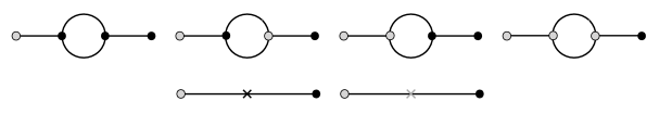
Figure 2: (Top) Connected one-loop contributions to the two-point correlation function in a $\lambda\phi^{3}$ theory. (Bottom) The corresponding $\delta_{m}$ and/or $\delta_{r}$ counterterm diagrams.

Let us now calculate the contribution from the cubic interaction in eq. (19). We first do a few manipulations to write this expression in a simpler form, that can then be calculated using Mathematica. We expand the Green’s functions in the loop, $G_{p}$ and $G_{|\vec{k}-\vec{p}|}$, in terms of $\theta$-functions, for example, $G_{p}^{++}(t_{1},t_{2})=G_{p}^{-+}(t_{1},t_{2})\theta(t_{1}-t_{2})+G_{p}^{+-}(t_{1},t_{2})\theta(t_{2}-t_{1})$, and similarly for $G_{p}^{--}(t_{1},t_{2})$ and the $|\vec{k}-\vec{p}|$ pieces, and introduce $\theta$-functions in the second and third lines using $\theta(t_{1}-t_{2})+\theta(t_{2}-t_{1})=1$. We next set the upper time integral $t_{f}$ to $t$, choosing $t>t^{\prime}$. This allows us to rewrite eq. (19) as

$$G_{k,\lambda\phi^{3}}^{-+}(t,t^{\prime})\ =\ -\frac{\lambda^{2}}{2}\int_{t_{1},t_{2}}\int_{\vec{p}}\Big{[}$$

$$\qquad\qquad G_{p}^{-+}(t_{1},t_{2})G_{|\vec{k}-\vec{p}|}^{-+}(t_{1},t_{2})G_{k}^{++}(t_{2},t^{\prime})\left\{G_{k}^{-+}(t,t_{1})-G_{k}^{+-}(t,t_{1})\right\}\theta(t_{1}-t_{2})$$

$$\qquad\qquad+\ G_{p}^{+-}(t_{1},t_{2})G_{|\vec{k}-\vec{p}|}^{+-}(t_{1},t_{2})G_{k}^{-+}(t,t_{1})\left\{G_{k}^{++}(t_{2},t^{\prime})-G_{k}^{-+}(t_{2},t^{\prime})\right\}\theta(t_{2}-t_{1})$$

$$\qquad\qquad+\ G_{p}^{-+}(t_{1},t_{2})G_{|\vec{k}-\vec{p}|}^{-+}(t_{1},t_{2})G_{k}^{+-}(t,t_{1})\left\{G_{k}^{-+}(t_{2},t^{\prime})-G_{k}^{++}(t_{2},t^{\prime})\right\}\theta(t_{2}-t_{1})$$

$$\qquad\qquad+\ G_{p}^{+-}(t_{1},t_{2})G_{|\vec{k}-\vec{p}|}^{+-}(t_{1},t_{2})G_{k}^{-+}(t_{2},t^{\prime})\left\{G_{k}^{+-}(t,t_{1})-G_{k}^{-+}(t,t_{1})\right\}\theta(t_{1}-t_{2})\Big{]}\,,\qquad$$ (24)

where $\int_{t_{i}}$ now stands for $\int_{t_{0}}^{t}\mathrm{d}t_{i}$. Now since the integrals are symmetric in $t_{1}$ and $t_{2}$, we can make the substitution $t_{1}\leftrightarrow t_{2}$ in the second and third terms, so that all four terms are proportional to $\theta(t_{1}-t_{2})$. We next expand the remaining $++$ Green’s functions in terms of $\theta$-functions as well and insert $\theta(t_{2}-t^{\prime})+\theta(t^{\prime}-t_{2})=1$ in appropriate places to write eq. (24) in the following form,

$$G_{k,\lambda\phi^{3}}^{-+}(t,t^{\prime}) = G_{k,\lambda\phi^{3},1}^{-+}(t,t^{\prime})+G_{k,\lambda\phi^{3},2}^{-+}(t,t^{\prime})+G_{k,\lambda\phi^{3},2}^{-+}(t^{\prime},t)\,,$$ (25)

where

$$G_{k,\lambda\phi^{3},1}^{-+}(t,t^{\prime}) = -\frac{\lambda^{2}}{2}\int_{t^{\prime}}^{t}\mathrm{d}t_{1}\int_{t^{\prime}}^{t_{1}}\mathrm{d}t_{2}\int_{\vec{p}}\Big{[}G_{p}^{-+}(t_{1},t_{2})G_{|\vec{k}-\vec{p}|}^{-+}(t_{1},t_{2})\big{\{}G_{k}^{-+}(t,t_{1})$$ (26)

$$\qquad-\ G_{k}^{+-}(t,t_{1})\big{\}}\left\{G_{k}^{-+}(t_{2},t^{\prime})-G_{k}^{+-}(t_{2},t^{\prime})\right\}\Big{]}\,,$$

$$G_{k,\lambda\phi^{3},2}^{-+}(t,t^{\prime}) = -\frac{\lambda^{2}}{2}\int_{t_{0}}^{t^{\prime}}\mathrm{d}t_{1}\int_{t_{0}}^{t_{1}}\mathrm{d}t_{2}\int_{\vec{p}}\Big{[}G_{p}^{-+}(t_{1},t_{2})G_{|\vec{k}-\vec{p}|}^{-+}(t_{1},t_{2})G_{k}^{-+}(t,t_{2})$$ (27)

$$\qquad\times\left\{G_{k}^{+-}(t_{1},t^{\prime})-G_{k}^{-+}(t_{1},t^{\prime})\right\}\Big{]}+\,{\rm c.c.}\,,$$

with ‘c.c.’ indicating the complex conjugate. We have essentially separated the contribution that is independent of the initial time $t_{0}$ from the one that depends on it. Before calculating the common loop integral, we will change $\int\mathrm{d}t_{1}\int\mathrm{d}t_{2}$ to $\int\mathrm{d}\tau\int\mathrm{d}\Delta$, where for the time integrals in eq. (26) we define $\tau=t_{1}-t^{\prime}$ and $\Delta=t_{1}-t_{2}$ and for the time integrals in eq. (27) we define $\tau=t_{1}-t_{0}$ and $\Delta=t_{1}-t_{2}$. We can also use the fact that the functions $G_{k}^{\pm\pm}(t,t^{\prime})$ in Minkowski, and for our choice of initial state, only depend on the difference of times $t-t^{\prime}$, so that we can write them as $G_{k}^{\pm\pm}(t-t^{\prime})$. Then eqs. (26) and (27) become

$$G_{k,\lambda\phi^{3},1}^{-+}(t,t^{\prime}) = -\frac{\lambda^{2}}{2}\int_{0}^{t-t^{\prime}}\mathrm{d}\tau\int_{0}^{\tau}\mathrm{d}\Delta\int_{\vec{p}}\Big{[}G_{p}^{-+}(\Delta)G_{|\vec{k}-\vec{p}|}^{-+}(\Delta)\big{\{}G_{k}^{-+}(t-t^{\prime}-\tau)$$ (28)

$$\qquad-\ G_{k}^{+-}(t-t^{\prime}-\tau)\big{\}}\left\{G_{k}^{-+}(\tau-\Delta)-G_{k}^{+-}(\tau-\Delta)\right\}\Big{]}\,,$$

$$G_{k,\lambda\phi^{3},2}^{-+}(t,t^{\prime}) = -\frac{\lambda^{2}}{2}\int_{0}^{t^{\prime}-t_{0}}\mathrm{d}\tau\int_{0}^{\tau}\mathrm{d}\Delta\int_{\vec{p}}\Big{[}G_{p}^{-+}(\Delta)G_{|\vec{k}-\vec{p}|}^{-+}(\Delta)G_{k}^{-+}(t-t_{0}-\tau+\Delta)$$ (29)

$$\qquad\times\left\{G_{k}^{-+}(t^{\prime}-t_{0}-\tau)-G_{k}^{+-}(t^{\prime}-t_{0}-\tau)\right\}\Big{]}+\,{\rm c.c.}\,.$$

The lower limit of all time integrals is now zero, where we will find a pole later. We next calculate the loop integral first that is common to both contributions and given by

$$I_{\lambda\phi^{3}}(k,\Delta)\ =\ \frac{\lambda^{2}}{2}\int_{\vec{p}}G_{p}^{-+}(\Delta)G_{|\vec{k}-\vec{p}|}^{-+}(\Delta)$$

$$\quad=\ \frac{\lambda^{2}}{2^{d+1}\pi^{d/2}\Gamma\left(d/2-1\right)}\frac{1}{k}\int_{0}^{\infty}\mathrm{d}p\int_{|k-p|}^{k+p}\mathrm{d}q\,p^{d-4}\left[1-\frac{\left(k^{2}+p^{2}-q^{2}\right)^{2}}{4k^{2}p^{2}}\right]^{d/2-2}e^{-i(p+q)\Delta}\,,\ \$$

(30)

where we have used $\int\mathrm{d}^{d}x=\frac{2\pi^{(d-1)/2}}{\Gamma[(d-1)/2]}\int_{0}^{\infty}\mathrm{d}x\int_{-1}^{1}\mathrm{d}\cos\theta\,x^{d-1}\sin^{d-3}\theta$, defined $q=|\vec{k}-\vec{p}|=\left(k^{2}+p^{2}-2kp\cos\theta\right)^{1/2}$, and changed the integral over $\cos\theta$ to $q$ using $\mathrm{d}\cos\theta=-\frac{q}{kp}\,\mathrm{d}q$. We have also restricted to the massless limit as mentioned earlier.

This is as far as we can get in the calculation of $G_{k,\lambda\phi^{3}}^{-+}$ (the one-loop correction to $G_{k}^{-+}$ from the $\lambda\phi^{3}$ interaction) without specifying the number of spacetime dimensions, and we will now specialize to $d=4$ or $d=6$.

(i) $\lambda\phi^{3}$ in 4D

We first set $d=4+\epsilon$, where $\epsilon$ is infinitesimal and serves to regulate the integrals as before. In this case, the coupling $\lambda$ has the dimensions of mass. The loop integral in eq. (30) does not, in fact, need a regulator if we convert $\Delta$ into a Euclidean time coordinate, and simply leads to poles in the Euclidean $\Delta$. We thus define $\Delta=-i\bar{\Delta}$ and use $\epsilon$ to regulate the $\bar{\Delta}$ integral, setting $d=4$ in the momentum integral. In other words, we take the fractional dimension to be solely in the time coordinate, leaving the number of spatial dimensions as an integer. Then eq. (30) becomes

$$I_{\lambda\phi^{3}}(k,\bar{\Delta}) = \frac{\lambda^{2}}{32\pi^{2}k}\int_{0}^{\infty}\mathrm{d}p\int_{|k-p|}^{k+p}\mathrm{d}q\,e^{-(p+q)\bar{\Delta}}$$ (31)

$$= \frac{\lambda^{2}}{2}\frac{e^{-k\bar{\Delta}}}{16\pi^{2}\bar{\Delta}}\,.$$

We now use this expression in eqs. (28) and (29), converting the $\Delta$ to $\bar{\Delta}$ and leaving the $\tau$ as is, which then become

$$G_{k,\lambda\phi^{3},1}^{-+}(t,t^{\prime}) = \frac{i\lambda^{2}\mu^{\epsilon}}{128\pi^{2}k^{2}}\frac{\pi^{(1+\epsilon)/2}}{\Gamma[(1+\epsilon)/2]}\int_{0}^{t-t^{\prime}}\mathrm{d}\tau\int_{0}^{i\tau}\mathrm{d}\bar{\Delta}\,\bar{\Delta}^{\epsilon}\bigg{[}\frac{e^{-k\bar{\Delta}}}{\bar{\Delta}}\Big{\{}e^{-ik(t-t^{\prime}-\tau)}$$ (32)

$$\qquad-\ e^{ik(t-t^{\prime}-\tau)}\Big{\}}\left\{e^{-ik(\tau+i\bar{\Delta})}-e^{ik(\tau+i\bar{\Delta})}\right\}\bigg{]}\,,$$

$$G_{k,\lambda\phi^{3},2}^{-+}(t,t^{\prime}) = \frac{i\lambda^{2}\mu^{\epsilon}}{128\pi^{2}k^{2}}\frac{\pi^{(1+\epsilon)/2}}{\Gamma[(1+\epsilon)/2]}\int_{0}^{t^{\prime}-t_{0}}\mathrm{d}\tau\int_{0}^{i\tau}\mathrm{d}\bar{\Delta}\,\bar{\Delta}^{\epsilon}\bigg{[}\frac{e^{-k\bar{\Delta}}}{\bar{\Delta}}\,e^{-ik(t-t_{0}-\tau-i\bar{\Delta})}$$ (33)

$$\qquad\times\left\{e^{-ik(t^{\prime}-t_{0}-\tau)}-e^{ik(t^{\prime}-t_{0}-\tau)}\right\}\Big{]}+\,{\rm c.c.}\,,$$

where, as before, $\mu$ is a parameter with dimensions of mass, introduced to keep the dimensions of $\lambda$ fixed. These integrals are straightforward to calculate. The result can be plugged into eq. (25) to obtain the contribution from the interaction to the one-loop two-point correlator in eq. (18). We can then perform a series expansion around $\epsilon=0$ to separate the finite piece from the UV-divergent piece that must be canceled by an appropriate choice of counterterms.

Let us first look at the finite (i.e. independent of $\epsilon$) part of $G_{k,\lambda\phi^{3}}^{-+}(t,t^{\prime})$ since this is the main result of the current section. We will call this the one-loop correction to $G_{k}^{-+}(t,t^{\prime})$ since all UV-divergent terms can be canceled by counterterms, as we will see later. We find that

$$G_{k,{\rm 1-loop}}^{-+}(t,t^{\prime})$$

$$\ \ =\ -\frac{i\lambda^{2}e^{-ik(t-t^{\prime})}(t-t^{\prime})}{128k^{2}\pi^{2}}\Bigg{[}1-\ln\left(\frac{2\pi\mu^{2}(t-t^{\prime})}{k}\right)-{\rm Ei}\left\{2ik(t-t_{0})\right\}+i\frac{\pi}{2}$$

$$\qquad\quad+\ e^{2ik(t-t^{\prime})}\Big{(}{\rm Ei}\left\{-2ik(t-t_{0})\right\}-{\rm Ei}\left\{-2ik(t-t^{\prime})\right\}\Big{)}\Bigg{]}$$

$$\qquad-\frac{i\lambda^{2}e^{-ik(t-t^{\prime})}(t^{\prime}-t_{0})}{128k^{2}\pi^{2}}\Bigg{[}2i\pi+{\rm Ei}\left\{-2ik(t^{\prime}-t_{0})\right\}-{\rm Ei}\left\{2ik(t-t_{0})\right\}$$

$$\qquad\quad+\ e^{2ik(t-t^{\prime})}\Big{(}{\rm Ei}\left\{-2ik(t-t_{0})\right\}-{\rm Ei}\left\{2ik(t^{\prime}-t_{0})\right\}+2i\pi\Big{)}\Bigg{]}$$

$$\qquad+\frac{\lambda^{2}e^{-ik(t-t^{\prime})}}{256k^{3}\pi^{2}}\Bigg{[}3+{\rm Ei}\left\{2ik(t-t_{0})\right\}+{\rm Ei}\left\{-2ik(t^{\prime}-t_{0})\right\}$$

$$\qquad\quad+\ 2\ln\left(\frac{4i\pi\mu^{2}(t-t^{\prime})}{2k}\right)+e^{2ik(t-t^{\prime})}\Big{(}1-2{\rm Ei}\left\{-2ik(t-t^{\prime})\right\}-i\pi+{\rm Ei}\left\{2ik(t^{\prime}-t_{0})\right\}$$

$$\qquad\quad+\ {\rm Ei}\left\{-2ik(t-t_{0})\right\}\Big{)}-e^{ik(t-t^{\prime})}\Big{(}2\cos\left\{k(t+t^{\prime}-2t_{0})\right\}\left(2+\gamma\right)$$

$$\qquad\quad+\ 2\cos\left\{k(t+t^{\prime}-2t_{0})\right\}\ln\left\{4\pi\mu^{2}(t-t_{0})(t^{\prime}-t_{0})\right\}+2\pi\sin\left\{k(t+t^{\prime}-2t_{0})\right\}\Big{)}\Bigg{]}\,,$$

(34)

where ${\rm Ei}(z)=\int_{-z}^{\infty}\mathrm{d}t\,\frac{e^{-t}}{t}$ is the (principal value of the) exponential integral, $\gamma$ is the Euler-Mascheroni constant, and we have used the MS renormalization scheme (we return to this point below). There are several interesting things to note about this expression. First, it vanishes in the limit $t=t^{\prime}=t_{0}$, as expected from our initial condition. Second, it is time translation invariant as long as we shift all times, including the initial time, by the same amount. Third, there is no IR issue despite the factor of $1/k^{3}$ outside, since the $k\rightarrow 0$ limit of eq. (34) in fact goes as $1/k$, similar to the free theory. Fourth, if we take the equal-time limit $t=t^{\prime}$, further take the late-time limit so that $t-t_{0}$ is bigger than any timescale in the problem, $\lambda(t-t_{0})\gg 1$, $k(t-t_{0})\gg 1$, and $\mu(t-t_{0})\gg 1$, and drop oscillatory terms by averaging over the late time interval, then we find that

$$\lim_{t\gg t_{0}}G_{k,{\rm 1-loop}}^{-+}(t,t) = \frac{\lambda^{2}}{128k^{3}\pi^{2}}\left[2-\gamma-\ln\left(\frac{\pi\mu^{2}}{k^{2}}\right)\right],$$ (35)

which does not exhibit any secular growth, consistent with the expectation that the (free theory) vacuum is stable under a $\lambda\phi^{3}$ interaction in Minkowski Chaykov:2022zro . And fifth, the late-time limit, such that all time differences $T=t-t_{0}$, $t^{\prime}-t_{0}$, and $t-t^{\prime}$ satisfy $\lambda T\gg 1$, $kT\gg 1$, and $\mu T\gg 1$, does exhibit secular growth with

$$\lim_{t\gg t^{\prime}\gg t_{0}}G_{k,{\rm 1-loop}}^{-+}(t,t^{\prime}) = \frac{\lambda^{2}(t-t^{\prime})e^{-ik(t-t^{\prime})}}{256k^{2}\pi^{2}}\left[-2i-\pi+2i\ln\left(\frac{2\pi\mu^{2}(t-t^{\prime})}{k}\right)\right].$$ (36)

This is consistent with what we find in our companion paper Chaykov:2022zro , where we use an in-out approach to directly obtain the late-time result, with differences that can be absorbed into the counterterms. As shown there, the Weisskopf-Wigner (WW) resummation method resums the late-time secular growth into exponential decay, consistent with the expectation that while the vacuum is stable in Minkowski, the one-particle state decays. Also note that the expression in eq. (36) goes as $(1/k^{2})\ln k$ in the $k\rightarrow 0$ limit, which still does not lead to an IR issue on converting to real space.

Let us next consider the UV-divergent piece of $G_{k,\lambda\phi^{3}}^{-+}(t,t^{\prime})$,

$$G_{k,\lambda\phi^{3},\epsilon}^{-+}(t,t^{\prime}) = \frac{\lambda^{2}e^{-ik(t-t^{\prime})}}{128\pi^{2}k^{3}\epsilon}\left[2+2ik(t-t^{\prime})-e^{2ik(t-t_{0})}-e^{-2ik(t^{\prime}-t_{0})}\right].$$ (37)

Comparing this to the $\delta_{m}$ and $\delta_{r}$ contributions in eqs. (22) and (23), we see that the UV-divergence can be fully canceled by choosing the counterterms to be

$$\delta_{m}\ =\ \frac{\lambda^{2}}{16\pi^{2}\epsilon}\,,\quad\delta_{r}\ =\ 0\,,$$ (38)

where we have used the MS renormalization scheme. Note that we do not need to add counterterms in the initial state, and so we can take $\delta A_{k}$ and $\delta B_{k}$ introduced in section 3 to both be zero.

(ii) $\lambda\phi^{3}$ in 6D

We next set $d=6+\epsilon$, so that $\lambda$ is dimensionless. As in the 4D case, we define $\Delta=-i\bar{\Delta}$ and use $\epsilon$ to regulate the $\bar{\Delta}$ integral, setting $d=6$ in the momentum integral. Now eq. (30) becomes

$$I_{\lambda\phi^{3}}(k,\bar{\Delta}) = \frac{\lambda^{2}}{128\pi^{3}k}\int_{0}^{\infty}\mathrm{d}p\int_{|k-p|}^{k+p}\mathrm{d}q\left[p^{2}-\frac{\left(k^{2}+p^{2}-q^{2}\right)^{2}}{4k^{2}}\right]e^{-(p+q)\bar{\Delta}}$$ (39)

$$= \frac{\lambda^{2}}{2}\frac{e^{-k\bar{\Delta}}\left(1+k\bar{\Delta}\right)}{192\pi^{3}\bar{\Delta}^{3}}\,.$$

Using this expression in eqs. (28) and (29), plugging the result into eq. (25), and series expanding around $\epsilon=0$ (the integrals converge for $\epsilon>2$ but we can analytically continue the result to smaller $\epsilon$), once again gives us the finite and UV-divergent pieces of the one-loop two-point correlator in eq. (18). The finite part of the one-loop correction is now given by

$$G_{k,{\rm 1-loop}}^{-+}(t,t^{\prime})\ =\ \frac{\lambda^{2}e^{-ik(t-t^{\prime})}}{3072\pi^{3}k}\Bigg{[}\gamma-i\pi-2\ln\left(\frac{2\pi^{3/2}\mu^{3}(t-t^{\prime})}{k^{2}}\right)-2\text{Ei}\left\{-2ik(t-t_{0})\right\}-2$$

$$\qquad-\ 2\text{Ei}\left\{-2ik(t^{\prime}-t_{0})\right\}+e^{2ik(t-t^{\prime})}\Bigg{(}\gamma+2i\pi+2\text{Ei}\left\{-2ik(t-t^{\prime})\right\}-2\text{Ei}\left\{-2ik(t-t_{0})\right\}$$

$$\qquad-\ 2\text{Ei}\left\{2ik(t^{\prime}-t_{0})\right\}-\ln\left(\frac{\pi\mu^{2}}{k^{2}}\right)\Bigg{)}\Bigg{]}\,,$$ (40)

where $\mu$ is again a parameter with dimensions of mass, introduced to keep the dimensions of $\lambda$ fixed. This expression shares the first four features mentioned after eq. (34), except for a subtlety when taking the $t=t^{\prime}=t_{0}$ limit. Once we set $t=t^{\prime}$ and take the limit as $t\rightarrow t_{0}$, we find a $\ln\{\mu(t-t_{0})\}$ divergence. This can be removed by choosing $\mu=1/(t-t_{0})$, this being the only scale left in the problem, and is likely related to the simultaneous appearance of non-zero initial state counterterms that we discuss below. Also, to show the equal-time late-time limit explicitly, if we set $t=t^{\prime}$, take $k(t-t_{0})\gg 1$ and $\mu(t-t_{0})\gg 1$ we find that

$$\lim_{t\gg t_{0}}G_{k,{\rm 1-loop}}^{-+}(t,t) = \frac{\lambda^{2}}{768k\pi^{3}}\left[\gamma-\ln\left(\frac{\pi\mu^{2}}{k^{2}}\right)\right],$$ (41)

which again does not exhibit any secular growth. The late-time limit of eq. (40), such that all time differences $T=t-t_{0}$, $t^{\prime}-t_{0}$, and $t-t^{\prime}$ satisfy $kT\gg 1$ and $\mu T\gg 1$, on the other hand, now exhibits secular growth that is logarithmic rather than linear in $t-t^{\prime}$,

$$\lim_{t\gg t^{\prime}\gg t_{0}}G_{k,{\rm 1-loop}}^{-+}(t,t^{\prime}) = -\frac{\lambda^{2}e^{-ik(t-t^{\prime})}}{1536\pi^{3}k}\ln\left\{\mu(t-t^{\prime})\right\}.$$ (42)

This is also consistent with what we find in our companion paper Chaykov:2022zro and, as shown there, the result can be resummed to yield a polynomial decay.

Lastly, let us look at the UV-divergent piece of $G_{k,\lambda\phi^{3}}^{-+}(t,t^{\prime})$,

$$G_{k,\lambda\phi^{3},\epsilon}^{-+}(t,t^{\prime}) = -\frac{\lambda^{2}e^{-ik(t-t^{\prime})}}{1536\pi^{3}k\epsilon}\left[e^{2ik(t-t^{\prime})}+3\right].$$ (43)

Comparing this to the $\delta_{m}$ and $\delta_{r}$ contributions in eqs. (22) and (23), we see that the UV-divergence is not fully canceled by these counterterms. Therefore, we need additional counterterms in the initial state in this case. To calculate the contributions from $\delta A_{k}$ and $\delta B_{k}$, we can treat the initial state action in eq. (15) as any other counterterm action, with the only difference that it is defined at the initial time. Then following steps very similar to those outlined in eqs. (20)-(23), we find that the additional counterterm contributions to $G_{k,{\rm 1-loop}}^{-+}(t,t^{\prime})$ are

$$G_{k,\delta A_{k}\phi^{2}}^{-+}(t,t^{\prime}) = \frac{i\delta A_{k}^{*}e^{ik(t+t^{\prime}-2t_{0})}}{4k^{2}}-\frac{i\delta A_{k}e^{-ik(t+t^{\prime}-2t_{0})}}{4k^{2}}\,,$$ (44)

$$G_{k,\delta B_{k}\phi^{2}}^{-+}(t,t^{\prime}) = -\frac{\delta B_{k}\cos\left[k(t-t^{\prime})\right]}{2k^{2}}\,.$$ (45)

Now we can start with fixing $\delta B_{k}$ so that it cancels the $e^{ik(t-t^{\prime})}$ part of the UV divergence in eq. (43), since this is the only counterterm that contains such a term. We can next choose $\delta_{r}$ so that it cancels the remaining piece proportional to $e^{-ik(t-t^{\prime})}$ and finally choose $\delta A_{k}$ to cancel any remaining divergences. This leads to the following choice of counterterms,

$$\delta_{m}\ =\ 0\,,\quad\delta_{r}\ =\ -\frac{\lambda^{2}}{384\pi^{3}\epsilon}\,,\quad\delta A_{k}\ =\ \frac{i\lambda^{2}k}{384\pi^{3}\epsilon}\,,\quad\delta B_{k}\ =\ -\frac{\lambda^{2}k}{384\pi^{3}\epsilon}\,.$$ (46)

An interesting point to note is that $\delta B_{k}$ is non-zero. Looking back at eq. (15), we see that this couples the $\phi^{+}$ and $\phi^{-}$ fields at the initial time, and therefore leads to mixing in the initial state. This is also confirmed by calculating the purity of the state, that is indeed less than unity if $\delta B_{k}$ is non-zero (the zeroth order $B_{k}$ vanishes for our choice of initial state).

4.2 $\lambda\phi^{4}$ in 4D

Let us next consider a $\lambda\phi^{4}$ interaction in $d$ dimensions, specializing to $d=4$ later in the calculation. Since the $\lambda\phi^{4}$ interaction does not generate a one-point expectation value, we can directly look at the two-point correlation, specifically $G_{k}^{-+}(t,t^{\prime})$ with $t>t^{\prime}$. We first calculate the one-loop correction to it that contributes at ${\cal O}(\lambda)$. The one-loop diagrams and the $\delta_{m}$ and $\delta_{r}$ counterterm diagrams are shown in fig. 3 and their contribution to $G_{k}^{-+}(t,t^{\prime})$ is

$$G_{k,{\rm 1-loop}}^{-+}(t,t^{\prime}) = G_{k,\lambda\phi^{4}}^{-+}(t,t^{\prime})+G_{k,\delta_{m}\phi^{2}}^{-+}(t,t^{\prime})+G_{k,\delta_{r}(\partial\phi)^{2}}^{-+}(t,t^{\prime})\,,$$ (47)

where

$$G_{k,\lambda\phi^{4}}^{-+}(t,t^{\prime}) = \frac{i\lambda}{2}\int_{t_{1}}\int_{\vec{p}}\Big{[}G_{k}^{-+}(t,t_{1})G_{p}^{++}(t_{1},t_{1})G_{k}^{++}(t_{1},t^{\prime})$$ (48)

$$\qquad-\ G_{k}^{--}(t,t_{1})G_{p}^{--}(t_{1},t_{1})G_{k}^{-+}(t_{1},t^{\prime})\Big{]}\,,$$

and the two counterterm contributions are the same as those of the previous subsection. On using the fact that all $G_{k}^{\pm\pm}(t,t)$ are the same, we see that the loop integral here is identical to that in eq. (17) for the $Y$ counterterm in the cubic theory. As found there, the loop integral vanishes in the massless limit that we are working in, and so eq. (48) also vanishes in this limit.

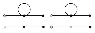
Figure 3: (Top) One-loop contributions to the two-point correlation function in a $\lambda\phi^{4}$ theory. (Bottom) The corresponding $\delta_{m}$ and/or $\delta_{r}$ counterterm diagrams.

Since the one-loop correction vanishes, we also calculate the two-loop correction to the two-point correlation. There are two types of two-loop diagrams, both contributing at ${\cal O}(\lambda^{2})$. The first set of diagrams, that we refer to as the snowman (‘sm’) diagrams, along with the corresponding $\delta_{m}$ and $\delta_{r}$ counterterm diagrams are shown in fig. 4 and the second set of diagrams, that we refer to as the sunset (‘ss’) diagrams, along with the corresponding $\delta_{m}$ and $\delta_{r}$ counterterm diagrams are shown in fig. 5. Their full contribution to $G_{k}^{-+}(t,t^{\prime})$ is

$$G_{k,{\rm 2-loop}}^{-+}(t,t^{\prime}) = G_{k,\lambda\phi^{4},{\rm sm}}^{-+}(t,t^{\prime})+G_{k,\delta_{m}\phi^{2},{\rm sm}}^{-+}(t,t^{\prime})+G_{k,\delta_{r}(\partial\phi)^{2},{\rm sm}}^{-+}(t,t^{\prime})$$ (49)

$$\quad+\ G_{k,\lambda\phi^{4},{\rm ss}}^{-+}(t,t^{\prime})+G_{k,\delta_{m}\phi^{2},{\rm ss}}^{-+}(t,t^{\prime})+G_{k,\delta_{r}(\partial\phi)^{2},{\rm ss}}^{-+}(t,t^{\prime})\,,$$

where the first line corresponds to the diagrams in fig. 4 and the second to those in fig. 5. The contribution from the snowman diagrams is

$$G_{k,\lambda\phi^{4},{\rm sm}}^{-+}(t,t^{\prime}) = -\frac{\lambda^{2}}{2}\int_{t_{1},t_{2}}\int_{\vec{p}_{1},\vec{p}_{2}}\Big{[}G_{k}^{-+}(t,t_{1})G_{p_{1}}^{++}(t_{1},t_{2})G_{p_{1}}^{++}(t_{1},t_{2})G_{p_{2}}^{++}(t_{2},t_{2})G_{k}^{++}(t_{1},t^{\prime})$$ (50)

$$\qquad-\ G_{k}^{-+}(t,t_{1})G_{p_{1}}^{+-}(t_{1},t_{2})G_{p_{1}}^{+-}(t_{1},t_{2})G_{p_{2}}^{--}(t_{2},t_{2})G_{k}^{++}(t_{1},t^{\prime})$$

$$\qquad-\ G_{k}^{--}(t,t_{1})G_{p_{1}}^{-+}(t_{1},t_{2})G_{p_{1}}^{-+}(t_{1},t_{2})G_{p_{2}}^{++}(t_{2},t_{2})G_{k}^{-+}(t_{1},t^{\prime})$$

$$\qquad+\ G_{k}^{--}(t,t_{1})G_{p_{1}}^{--}(t_{1},t_{2})G_{p_{1}}^{--}(t_{1},t_{2})G_{p_{2}}^{--}(t_{2},t_{2})G_{k}^{-+}(t_{1},t^{\prime})\Big{]}\,.$$

The $\vec{p}_{2}$ integrals here are of the same form as encountered in the one-loop correction and eq. (17), and therefore, the snowman contribution also vanishes in the massless limit.

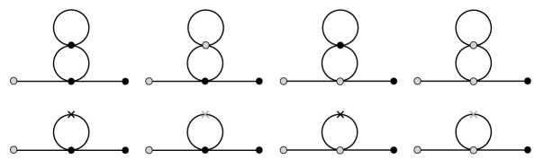
Figure 4: (Top) Connected two-loop contributions of the ‘snowman’ type to the two-point correlation function in a $\lambda\phi^{4}$ theory. (Bottom) The corresponding $\delta_{m}$ and/or $\delta_{r}$ counterterm diagrams.

The only nonzero correction to the two-point correlation comes from the sunset diagrams and is given by

$$G_{k,\lambda\phi^{4},{\rm ss}}^{-+}(t,t^{\prime})\ =\ -\frac{\lambda^{2}}{6}\int_{t_{1},t_{2}}\int_{\vec{p}_{1},\vec{p}_{2}}\Big{[}$$

$$\qquad\qquad G_{k}^{-+}(t,t_{1})G_{p_{1}}^{++}(t_{1},t_{2})G_{p_{2}}^{++}(t_{1},t_{2})G_{|\vec{k}-\vec{p}_{1}-\vec{p_{2}}|}^{++}(t_{1},t_{2})G_{k}^{++}(t_{2},t^{\prime})$$

$$\qquad\qquad-\ G_{k}^{-+}(t,t_{1})G_{p_{1}}^{+-}(t_{1},t_{2})G_{p_{2}}^{+-}(t_{1},t_{2})G_{|\vec{k}-\vec{p}_{1}-\vec{p_{2}}|}^{+-}(t_{1},t_{2})G_{k}^{-+}(t_{2},t^{\prime})$$

$$\qquad\qquad-\ G_{k}^{--}(t,t_{1})G_{p_{1}}^{-+}(t_{1},t_{2})G_{p_{2}}^{-+}(t_{1},t_{2})G_{|\vec{k}-\vec{p}_{1}-\vec{p_{2}}|}^{-+}(t_{1},t_{2})G_{k}^{++}(t_{2},t^{\prime})$$

$$\qquad\qquad+\ G_{k}^{--}(t,t_{1})G_{p_{1}}^{--}(t_{1},t_{2})G_{p_{2}}^{--}(t_{1},t_{2})G_{|\vec{k}-\vec{p}_{1}-\vec{p_{2}}|}^{--}(t_{1},t_{2})G_{k}^{-+}(t_{2},t^{\prime})\Big{]}\,.$$ (51)

To solve this, we first perform the same manipulations as those in the previous subsection. In fact, we can borrow many of the expressions that we had there, noticing that eq. (51) can simply be obtained from eq. (19) by making the replacement

$$-\frac{\lambda^{2}}{2}\int_{\vec{p}}G_{p}^{ab}(t_{1},t_{2})G_{|\vec{k}-\vec{p}|}^{ab}(t_{1},t_{2})\rightarrow-\frac{\lambda^{2}}{6}\int_{\vec{p}_{1}}\int_{\vec{p}_{2}}G_{p_{1}}^{ab}(t_{1},t_{2})G_{p_{2}}^{ab}(t_{1},t_{2})G_{|\vec{k}-\vec{p}_{1}-\vec{p}_{2}|}^{ab}(t_{1},t_{2})\,.\quad\ \$$ (52)

for any $\pm$ indices $a$ and $b$. We can, therefore, write the sunset contribution in a form analogous to eq. (25) of the previous subsection,

$$G_{k,\lambda\phi^{4},{\rm ss}}^{-+}(t,t^{\prime}) = G_{k,\lambda\phi^{4},{\rm ss},1}^{-+}(t,t^{\prime})+G_{k,\lambda\phi^{4},{\rm ss},2}^{-+}(t,t^{\prime})+G_{k,\lambda\phi^{4},{\rm ss},2}^{-+}(t^{\prime},t)\,,$$ (53)

where $G_{k,\lambda\phi^{4},{\rm ss},1}^{-+}(t,t^{\prime})$ and $G_{k,\lambda\phi^{4},{\rm ss},2}^{-+}(t,t^{\prime})$, given below for clarity, are obtained from eqs. (26) and (27), respectively, on making the replacement of eq. (52),

$$G_{k,\lambda\phi^{4},{\rm ss},1}^{-+}(t,t^{\prime}) = -\frac{\lambda^{2}}{6}\int_{t^{\prime}}^{t}\mathrm{d}t_{1}\int_{t^{\prime}}^{t_{1}}\mathrm{d}t_{2}\int_{\vec{p}_{1}}\int_{\vec{p}_{2}}\Big{[}G_{p_{1}}^{-+}(t_{1},t_{2})G_{p_{2}}^{-+}(t_{1},t_{2})G_{|\vec{k}-\vec{p}_{1}-\vec{p}_{2}|}^{-+}(t_{1},t_{2})$$ (54)

$$\qquad\times\ \big{\{}G_{k}^{-+}(t,t_{1})-G_{k}^{+-}(t,t_{1})\big{\}}\left\{G_{k}^{-+}(t_{2},t^{\prime})-G_{k}^{+-}(t_{2},t^{\prime})\right\}\Big{]}\,,$$

$$G_{k,\lambda\phi^{4},{\rm ss},2}^{-+}(t,t^{\prime}) = -\frac{\lambda^{2}}{6}\int_{t_{0}}^{t^{\prime}}\mathrm{d}t_{1}\int_{t_{0}}^{t_{1}}\mathrm{d}t_{2}\int_{\vec{p}_{1}}\int_{\vec{p}_{2}}\Big{[}G_{p_{1}}^{-+}(t_{1},t_{2})G_{p_{2}}^{-+}(t_{1},t_{2})G_{|\vec{k}-\vec{p}_{1}-\vec{p}_{2}|}^{-+}(t_{1},t_{2})$$ (55)

$$\qquad\times\ G_{k}^{-+}(t,t_{2})\left\{G_{k}^{+-}(t_{1},t^{\prime})-G_{k}^{-+}(t_{1},t^{\prime})\right\}\Big{]}+\,{\rm c.c.}\,.$$

We can change $\int\mathrm{d}t_{1}\int\mathrm{d}t_{2}$ to $\int\mathrm{d}\tau\int\mathrm{d}\Delta$ and write the Green’s functions in terms of a single time variable as before. Also setting the mass to zero and the number of spatial dimensions to three, the loop integral that needs to be solved is then given by

$$I_{\lambda\phi^{4}}(k,\Delta) = \frac{\lambda^{2}}{6}\int_{\vec{p}_{1}}\int_{\vec{p}_{2}}G_{p_{1}}^{-+}(\Delta)G_{p_{2}}^{-+}(\Delta)G_{|\vec{k}-\vec{p}_{1}-\vec{p}_{2}|}^{-+}(\Delta)$$ (56)

$$= \frac{\lambda^{2}}{768\pi^{4}k}\int_{0}^{\infty}\mathrm{d}p_{1}\int_{|k-p_{1}|}^{k+p_{1}}\mathrm{d}q_{1}\int_{0}^{\infty}\mathrm{d}p_{2}\int_{|q_{1}-p_{2}|}^{q_{1}+p_{2}}\mathrm{d}q_{2}\,e^{-i\left(p_{1}+p_{2}+q_{2}\right)\Delta}\,,$$

where we have defined $\vec{q}_{1}=\vec{k}-\vec{p}_{1}$ and $\vec{q}_{2}=\vec{q}_{1}-\vec{p}_{2}$, so that $q_{1}=\left(k^{2}+p_{1}^{2}-2kp_{1}\cos\theta_{1}\right)^{1/2}$ and $q_{2}=\left(q_{1}^{2}+p_{2}^{2}-2q_{1}p_{2}\cos\theta_{2}\right)^{1/2}$, and changed the integrals over $\cos\theta_{1}$ and $\cos\theta_{2}$ to $q_{1}$ and $q_{2}$ using $\mathrm{d}\cos\theta_{1}=-\frac{q_{1}}{kp_{1}}\,\mathrm{d}q_{1}$ and $\mathrm{d}\cos\theta_{2}=-\frac{q_{2}}{q_{1}p_{2}}\,\mathrm{d}q_{2}$, respectively.

Figure 5: (Top) Connected two-loop contributions of the ‘sunset’ type to the two-point correlation function in a $\lambda\phi^{4}$ theory. (Bottom) The corresponding $\delta_{m}$ and/or $\delta_{r}$ counterterm diagrams.

In order to regulate the integrals, we define a Euclidean time coordinate $\Delta=-i\bar{\Delta}$ and set $d=4+\epsilon$, absorbing the fractional dimension fully into the time coordinate, so that the number of spatial dimensions is still three. The integrals in eq. (56) can then be performed easily and we find that

$$I_{\lambda\phi^{4}}(k,\bar{\Delta}) = \frac{\lambda^{2}}{6}\frac{e^{-k\bar{\Delta}}\left(1+k\bar{\Delta}\right)}{256\pi^{4}\bar{\Delta}^{3}}\,.$$ (57)

Notice that this is exactly the same (up to a constant) as what we found for $\lambda\phi^{3}$ in 6D, in eq. (39), with both interactions sharing the fact that $\lambda$ is dimensionless. We can, therefore, directly write the contribution from the sunset diagrams using eq. (40) and we find that the finite part of the two-loop correction to the two-point correlation is given by

$$G_{k,{\rm 2-loop}}^{-+}(t,t^{\prime})\ =\ \frac{\lambda^{2}e^{-ik(t-t^{\prime})}}{12288\pi^{4}k}\Bigg{[}\gamma-i\pi-2\ln\left(\frac{2\pi^{3/2}\mu^{3}(t-t^{\prime})}{k^{2}}\right)-2\text{Ei}\left\{-2ik(t-t_{0})\right\}-2$$

$$\qquad-\ 2\text{Ei}\left\{-2ik(t^{\prime}-t_{0})\right\}+e^{2ik(t-t^{\prime})}\Bigg{(}\gamma+2i\pi+2\text{Ei}\left\{-2ik(t-t^{\prime})\right\}-2\text{Ei}\left\{-2ik(t-t_{0})\right\}$$

$$\qquad-\ 2\text{Ei}\left\{2ik(t^{\prime}-t_{0})\right\}-\ln\left(\frac{\pi\mu^{2}}{k^{2}}\right)\Bigg{)}\Bigg{]}\,.$$ (58)

The qualitative behavior of the loop correction matches what we found for $\lambda\phi^{3}$ in 6D, eq. (40). Similar to what we found there, the equal-time late-time limit with $t=t^{\prime}$, $k(t-t_{0})\gg 1$, and $\mu(t-t_{0})\gg 1$, does not exhibit any secular growth,

$$\lim_{t\gg t_{0}}G_{k,{\rm 1-loop}}^{-+}(t,t) = \frac{\lambda^{2}}{3072k\pi^{4}}\left[\gamma-\ln\left(\frac{\pi\mu^{2}}{k^{2}}\right)\right],$$ (59)

while the late-time limit, with all time differences $T=t-t_{0}$, $t^{\prime}-t_{0}$, and $t-t^{\prime}$ satisfying $kT\gg 1$ and $\mu T\gg 1$, exhibits secular growth,

$$\lim_{t\gg t^{\prime}\gg t_{0}}G_{k,{\rm 2-loop}}^{-+}(t,t^{\prime}) = -\frac{\lambda^{2}e^{ik(t-t^{\prime})}}{6144\pi^{4}k}\ln\left\{\mu(t-t^{\prime})\right\}.$$ (60)

This again matches what we find in Chaykov:2022zro and, as shown there, the result can be resummed into a polynomial decay.

Lastly, let us consider the UV-divergent piece of $G_{k,\lambda\phi^{4},{\rm ss}}^{-+}(t,t^{\prime})$ that is given by

$$G_{k,\lambda\phi^{4},{\rm ss},\epsilon}^{-+}(t,t^{\prime}) = -\frac{\lambda^{2}e^{-ik(t-t^{\prime})}}{6144\pi^{4}k\epsilon}\left[e^{2ik(t-t^{\prime})}+3\right].$$ (61)

This is again fully canceled by a choice of counterterms similar to that in eq. (46),

$$\delta_{m}\ =\ 0\,,\quad\delta_{r}\ =\ -\frac{\lambda^{2}}{1536\pi^{4}\epsilon}\,,\quad\delta A_{k}\ =\ \frac{i\lambda^{2}k}{1536\pi^{4}\epsilon}\,,\quad\delta B_{k}\ =\ -\frac{\lambda^{2}k}{1536\pi^{4}\epsilon}\,,$$ (62)

with non-vanishing counterterms in the initial state.

5 Discussion

Loop corrections in quantum field theories away from equilibrium exhibit UV divergences beyond those that can be absorbed in standard counterterms in the dynamics. In this paper, we were interested in loop corrections to the unequal-time two-point correlator in different massless self-interacting scalar quantum field theories on a Minkowski background, taking particular care of the counterterms that are needed to cancel all UV divergences. We found finite-time perturbative results using the techniques of in-in perturbation theory, starting the evolution at a finite initial time $t_{0}$ in the free theory’s ground state and allowing for Gaussian corrections to the initial state due to the interaction.

We first considered a $\lambda\phi^{3}$ interaction in 4D, where $\lambda$ has the dimensions of mass, and found that standard counterterms in the dynamics were sufficient to cancel the UV divergences. We next considered two interactions where $\lambda$ is dimensionless, namely a $\lambda\phi^{3}$ interaction in 6D and a $\lambda\phi^{4}$ interaction in 4D. In both cases, we needed additional counterterms in the initial state to cancel all UV divergences. Such additional counterterms are expected to arise due to initial-time singularities that are associated with turning on an interaction at a finite initial time Calzetta:2008 ; Baacke:1997zz ; Baacke:1999ia ; Collins:2005nu ; Collins:2014qna . It is interesting to note, however, that we needed additional counterterms only for the two interactions that have a dimensionless $\lambda$ and are thus marginal. This may indicate a higher degree of entanglement between low and high energy modes for such interactions, along the lines of the results in Balasubramanian:2011wt . Interpreting renormalization as tracing out high energy modes would then suggest that the initial state should receive corrections that make it mixed, which is what we find with a non-zero $\delta B$.

For all interactions, we also found that perturbative corrections to the two-point correlator diverge in the late-time limit. In the case of $\lambda\phi^{3}$ in 4D, we found that the result grows linearly in time, while in the cases of $\lambda\phi^{3}$ in 6D and $\lambda\phi^{4}$ in 4D, we found that it grows logarithmically in time. As shown in our companion paper Chaykov:2022zro , the WW resummation method exponentiates the late-time result, so that the two-point correlator instead decays exponentially and polynomially, respectively. Lastly, we note again that we restricted to the massless limit as this allowed for analytical calculations. We further left our results in terms of an arbitrary renormalization parameter $\mu$ since we were primarily interested in the UV renormalization and late-time behavior of correlation functions in this paper.

- (1) J.S. Schwinger, Brownian motion of a quantum oscillator, J.Math.Phys. 2 (1961) 407.
- (2) K.T. Mahanthappa, Multiple production of photons in quantum electrodynamics, Phys.Rev. 126 (1962) 329.
- (3) P.M. Bakshi and K.T. Mahanthappa, Expectation value formalism in quantum field theory. 1., J.Math.Phys. 4 (1963) 1.
- (4) L.P. Kadanoff and G. Baym, Quantum Statistical Mechanics, W. A. Benjamin, Inc., New York (1962).
- (5) P.M. Bakshi and K.T. Mahanthappa, Expectation value formalism in quantum field theory. 2., J.Math.Phys. 4 (1963) 12.
- (6) L.V. Keldysh, Diagram technique for nonequilibrium processes, Zh.Eksp.Teor.Fiz. 47 (1964) 1515.
- (7) R.D. Jordan, Effective field equations for expectation values, Phys.Rev. D33 (1986) 444.
- (8) E. Calzetta and B.L. Hu, Closed time path functional formalism in curved space-time: application to cosmological back reaction problems, Phys.Rev. D35 (1987) 495.
- (9) E.A. Calzetta and B.-L.B. Hu, Nonequilibrium quantum field theory, Cambridge University Press (2008).
- (10) J. Baacke, K. Heitmann and C. Patzold, On the choice of initial states in nonequilibrium dynamics, Phys. Rev. D 57 (1998) 6398 [hep-th/9711144].
- (11) J. Baacke, D. Boyanovsky and H.J. de Vega, Initial time singularities in nonequilibrium evolution of condensates and their resolution in the linearized approximation, Phys. Rev. D 63 (2001) 045023 [hep-ph/9907337].
- (12) H. Collins and R. Holman, Renormalization of initial conditions and the trans-Planckian problem of inflation, Phys. Rev. D 71 (2005) 085009 [hep-th/0501158].
- (13) H. Collins, R. Holman and T. Vardanyan, Renormalizing an initial state, JHEP 10 (2014) 124 [1408.4801].
- (14) S. Chaykov, N. Agarwal, S. Bahrami and R. Holman, Loop corrections in Minkowski spacetime away from equilibrium 1: Late-time resummations, 2206.11288.
- (15) J. Berges, Introduction to nonequilibrium quantum field theory, AIP Conf. Proc. 739 (2005) 3 [hep-ph/0409233].
- (16) A. Kamenev, Field theory of non-equilibrium systems, Cambridge University Press (2011).
- (17) S. Weinberg, Quantum contributions to cosmological correlations, Phys. Rev. D72 (2005) 043514 [hep-th/0506236].
- (18) N. Agarwal and Y.-Z. Chu, Initial value formulation of a quantum damped harmonic oscillator, In preparation.
- (19) N. Agarwal, R. Holman, A.J. Tolley and J. Lin, Effective field theory and non-Gaussianity from general inflationary states, JHEP 1305 (2013) 085 [1212.1172].
- (20) X. Chen, Y. Wang and Z.-Z. Xianyu, Loop corrections to standard model fields in inflation, JHEP 08 (2016) 051 [1604.07841].
- (21) V. Balasubramanian, M.B. McDermott and M. Van Raamsdonk, Momentum-space entanglement and renormalization in quantum field theory, Phys. Rev. D 86 (2012) 045014 [1108.3568].