Information-Thermodynamic Bound on Information Flow in Turbulent Cascade

Abstract

We investigate the nature of information flow in turbulence from an information-thermodynamic viewpoint. For the fully developed three-dimensional fluid turbulence described by the fluctuating Navier–Stokes equation, we prove that information of large-scale eddies is transferred to small scales along with the energy cascade. We numerically illustrate our findings using a shell model and further show that in the inertial range, the intensity of the information flow is nearly constant and can be scaled by the large-eddy turnover time. Our numerical results also suggest that the corresponding information-thermodynamic efficiency is quite low compared to other typical information processing systems such as Maxwell’s demon. These findings provide a new perspective on how universality and intermittency of turbulent fluctuations emerge at small scales.

I Introduction

Turbulence is characterized by the interference of fluctuations between disparate space-time scales. Despite its seemingly complicated and unpredictable nature, universal laws are hidden behind the disordered fluid motion. For example, in fully developed three-dimensional turbulence, the energy spectrum exhibits the Kolmogorov spectrum $E(k)\propto k^{-5/3}$ at scales much smaller than the energy injection scale [1, 2, 3, 4, 5]. The Kolmogorov spectrum is universal in the sense that it is independent of the details of the large scales, such as the boundary conditions or the mechanism of the external stirring. Furthermore, in addition to the energy spectrum, which corresponds to the second-order moments of the velocity field, the higher-order moments also exhibit universal scaling laws [4, 6]. Such remarkable universality of turbulent fluctuations at small scales is believed to be induced by the energy cascade process, where the energy is transferred conservatively from large to small scales. More specifically, there is a common intuitive picture that the universal statistical properties emerge at small scales because “information” about the details of the large scales is lost in the chaotic stepwise cascade process [5, 7, 8].

Somewhat contrary to this intuitive picture, some numerical and experimental observations suggest that the small-scale eddies do not “forget” about the large scales. For example, it is known that fluctuations of small-scale quantities (e.g., the energy dissipation rate) follow those of large-scale quantities (e.g., the energy injection rate) with a time lag along with the energy cascade [9, 10, 11]. This time lag is on the order of the large-eddy turnover time, which is the characteristic time scale for the largest eddies to be stretched into smaller eddies. Another example is the chaos synchronization of small-scale motions induced by the energy cascade, where the small-scale velocity field is slaved to the chaotic dynamics of the large-scale velocity field [12, 13, 14, 15, 16]. Moreover, small-scale intermittency can also be regarded as such an example because it implies that the turbulent fluctuations grow in each cascade step and thus “remember” the large scales [4, 8, 7]. These phenomena suggest that information about the large-scale fluctuations is not lost in the cascade process, but rather is transferred to small scales.

In order to deepen our understanding of the generation mechanism of universality and intermittency of turbulent fluctuations, it is thus desirable to reveal the nature of the information transfer across scales associated with the energy cascade. As a first step toward this end, here we aim to prove that information of turbulent fluctuations is transferred from large to small scales in fully developed three-dimensional fluid turbulence. While turbulence has been studied in various contexts from information-theoretic perspectives in recent decades [17, 18, 19, 20, 21, 22, 23, 24, 25, 26, 27, 28], no previous studies have theoretically shown that information flows across scales along with turbulent cascade.

For this purpose, we employ information thermodynamics, which is a thermodynamic framework for information flow between interacting subsystems [29, 30, 31]. While information thermodynamics has its origins in the thought experiment of Maxwell’s demon, it has recently been applied to information processing at the cellular level in biological systems [32, 33, 34, 35, 36] and even to deterministic chemical reaction networks [37]. By applying information thermodynamics to turbulence, we can clearly define the concept of “information” as a quantity closely related to thermodynamic quantities and obtain universal constraints on the flow of the information. Note that information thermodynamics requires us to use a thermodynamically consistent model that includes thermal fluctuations, i.e., fluctuating hydrodynamic equations [38, 39]. To put it another way, this approach also enables us to investigate the effects of thermal fluctuations on turbulence dynamics, which has recently been intensively investigated [40, 41, 42, 43, 44, 45, 46].

In this paper, we prove that information of turbulent fluctuations is transferred from large to small scales along with the energy cascade. We emphasize that our main results, [Ineqs. (25) and (26)], are exact and universal relations, independent of the details of the flow under consideration. While we derive these relations for the fluctuating Navier–Stokes equation, our results are valid for various turbulence models, including shell models. We numerically illustrate our findings using the Sabra shell model and further show that in the inertial range, the intensity of the information flow is nearly constant and can be scaled by the large-eddy turnover time [Eq. (54)]. This observation suggests that the information of large-scale turbulent fluctuations is transferred to small scales with nearly constant intensity by the energy cascade process. Thus, our results challenge the conventional intuitive picture of how universality emerges at small scales. Moreover, our numerical results suggest that the corresponding information-thermodynamic efficiency is quite low compared to other typical information processing systems such as Maxwell’s demon. This implies that transferring information from large to small scales involves enormous thermodynamic costs, indicating the poor performance of turbulence as an information processing system.

This paper is organized as follows. In Sec. II, we introduce the fluctuating Navier–Stokes equation and its corresponding Fokker–Planck equation. In Sec. III, we briefly review some basic properties of fully developed turbulence described by the fluctuating Navier–Stokes equation. In Sec. IV, we introduce the two information-theoretic quantities that are important in describing our main result: mutual information and information flow. Then, in Sec. V, we explain our main result on the information flow in turbulence and its derivation. In the derivation, we first formulate the second law of thermodynamics for the fluctuating Navier–Stokes equation and then derive the second law of information thermodynamics. Section VI presents a numerical demonstration of our main result. By introducing the concept of information-thermodynamic efficiency, we show that it is quite low in turbulence compared to other typical information processing systems. We further show that in the inertial range, the intensity of the information flow is nearly constant and can be scaled by the large-eddy turnover time. In Sec. VII, we summarize our findings with some remarks and future perspectives. The appendices contain details of the derivations and numerical simulations.

II Setup

While our results are valid for various thermodynamically consistent turbulence models, we focus on the fluctuating Navier–Stokes equation except for Sec. VI, where we numerically illustrate our main result by using a shell model. We consider an incompressible fluid with constant mass density $\rho$, temperature $T$, and kinematic viscosity $\nu$, confined in a cube with periodic boundary conditions $\Omega=L\mathbb{T}^{3}$. Let ${\bm{u}}({\bm{x}},t)=(u^{x}({\bm{x}},t),u^{y}({\bm{x}},t),u^{z}({\bm{x}},t))$ be the fluid velocity at position ${\bm{x}}\in\Omega$ and time $t\in\mathbb{R}$. Hereafter, we often omit the argument $t$ to simplify the notation. The time evolution of the velocity field ${\bm{u}}$ is described by the fluctuating Navier–Stokes equation [38, 39, 42, 43]:

$$\partial_{t}{\bm{u}}+{\bm{u}}\cdot\nabla{\bm{u}}=-\nabla p+\nu\nabla^{2}{\bm{u}}+{\bm{f}}+\nabla\cdot\mathsf{s}$$ (1)

with the incompressibility condition $\nabla\cdot{\bm{u}}=0$, where $p$ denotes the kinematic pressure, ${\bm{f}}$ represents the external force per unit mass, which, without loss of generality, is assumed to be divergence-free. We further assume that ${\bm{f}}$ acts only at large scales, i.e., it is supported in Fourier space at low wave numbers $\sim k_{f}$. In the last term on the right-hand side of (1), $\mathsf{s}$ denotes a thermal fluctuating stress prescribed as a zero-mean Gaussian random field that satisfies

$$\langle\mathsf{s}^{ab}({\bm{x}},t)\mathsf{s}^{cd}({\bm{x}}^{\prime},t^{\prime})\rangle =\dfrac{2\nu k_{\mathrm{B}}T}{\rho}\left(\delta^{ac}\delta^{bd}+\delta^{ad}\delta^{bc}-\dfrac{2}{3}\delta^{ab}\delta^{cd}\right)$$

$$\qquad\times\delta^{3}({\bm{x}}-{\bm{x}}^{\prime})\delta(t-t^{\prime}),$$ (2)

where $a,b,c,d\in\{x,y,z\}$ and $\delta^{ab}$ denotes the Kronecker delta, which is $1$ if $a=b$, and zero otherwise. Here, the prefactor $2\nu k_{\mathrm{B}}T/\rho$, where $k_{\mathrm{B}}$ denotes the Boltzmann constant, is chosen according to the fluctuation-dissipation relation of the second kind [47, 48] so that the model (1) is thermodynamically consistent [49].

Let $\hat{\bm{u}}_{\bm{k}}$ be the Fourier mode of the velocity field with wave vector ${\bm{k}}\in(2\pi/L)\mathbb{Z}^{3}$ defined as

$$\hat{{\bm{u}}}_{\bm{k}}=\dfrac{1}{V}\int_{\Omega}d^{3}{\bm{x}}e^{-i{\bm{k}}\cdot{\bm{x}}}{\bm{u}}({\bm{x}}),$$ (3)

where $V:=L^{3}$ denotes the volume of the fluid. Here, we note that the fluctuating hydrodynamics describes fluid motions at the mesoscopic level [38, 39]. In other words, there is a cutoff wave number $\Lambda$ such that $\ell^{-1}_{\mathrm{macro}}\ll\Lambda\ll\ell^{-1}_{\mathrm{micro}}$, where $\ell_{\mathrm{macro}}$ denotes the macroscopic length scale characterizing the macroscopic behaviors and $\ell_{\mathrm{micro}}$ denotes the microscopic length scale, such as the molecular size, the interaction length, or the mean free path [43]. In the following, we shall assume that the summation over wave vectors $\sum_{\bm{k}}$ means the summation up to the cutoff wave number $\sum_{|{\bm{k}}|<\Lambda}$. Because of the reality condition $\hat{\bm{u}}^{*}_{\bm{k}}=\hat{\bm{u}}_{-{\bm{k}}}$, only the modes ${\bm{u}}_{\bm{k}}$ whose wave vector lies in the half-set

$$\mathcal{K}^{+}:=\begin{Bmatrix}&k^{x}>0&\text{or}\\ {\bm{k}}:&k^{y}>0&\text{if}\quad k^{x}=0\quad\text{or}\\ &k^{z}\geq 0&\text{if}\quad k^{x}=k^{y}=0\end{Bmatrix}$$ (4)

are independent (for a schematic of this set, see Fig. 1 in Sec. IV). Then, the fluctuating Navier–stokes equation (1) can be rewritten as stochastic differential equations for $\hat{\bm{u}}:=\{\hat{\bm{u}}_{\bm{k}}|{\bm{k}}\in\mathcal{K}^{+}\}$ and the complex-conjugate variables $\hat{\bm{u}}^{*}:=\{\hat{\bm{u}}^{*}_{\bm{k}}|{\bm{k}}\in\mathcal{K}^{+}\}$ (see Appendix A for the derivation):

$$\partial_{t}\hat{\bm{u}}_{\bm{k}} ={\bm{B}}_{\bm{k}}(\hat{\bm{u}},\hat{\bm{u}}^{*})-\nu k^{2}\hat{\bm{u}}_{\bm{k}}+\hat{\bm{f}}_{\bm{k}}+\sqrt{\dfrac{2\nu k^{2}k_{\mathrm{B}}T}{\rho}}\hat{\bm{\xi}}_{\bm{k}},$$ (5)

$$\partial_{t}\hat{\bm{u}}^{*}_{\bm{k}} ={\bm{B}}^{*}_{\bm{k}}(\hat{\bm{u}},\hat{\bm{u}}^{*})-\nu k^{2}\hat{\bm{u}}^{*}_{\bm{k}}+\hat{\bm{f}}^{*}_{\bm{k}}+\sqrt{\dfrac{2\nu k^{2}k_{\mathrm{B}}T}{\rho}}\hat{\bm{\xi}}^{*}_{\bm{k}}.$$ (6)

Here, ${\bm{B}}_{\bm{k}}(\hat{\bm{u}},\hat{\bm{u}}^{*})$ denotes the nonlinear term

$$B^{a}_{\bm{k}}(\hat{\bm{u}},\hat{\bm{u}}^{*}):=-ik^{c}\left(\delta^{ab}-\dfrac{k^{a}k^{b}}{k^{2}}\right)\sum_{{\bm{p}}+{\bm{q}}={\bm{k}}}\hat{u}^{b}_{\bm{p}}\hat{u}^{c}_{\bm{q}},$$ (7)

where $k:=|{\bm{k}}|$, and $\hat{\bm{\xi}}_{\bm{k}}$ denotes the zero-mean white Gaussian noise that satisfies $\hat{\bm{\xi}}^{*}_{\bm{k}}=\hat{\bm{\xi}}_{-{\bm{k}}}$, ${\bm{k}}\cdot\hat{\bm{\xi}}_{\bm{k}}=0$, and

$$\langle\hat{\xi}^{a}_{\bm{k}}(t)\hat{\xi}^{b*}_{{\bm{k}}^{\prime}}(t^{\prime})\rangle=\dfrac{1}{V}\left(\delta^{ab}-\dfrac{k^{a}k^{b}}{k^{2}}\right)\delta_{{\bm{k}},{\bm{k}}^{\prime}}\delta(t-t^{\prime}).$$ (8)

Note that the wave vectors ${\bm{p}}$ and ${\bm{q}}$, which are summed over in (7), may not belong to the half-set $\mathcal{K}^{+}$. If ${\bm{p}}\notin\mathcal{K}^{+}$, then $\hat{\bm{u}}_{\bm{p}}$ should be interpreted instead as $\hat{\bm{u}}^{*}_{-{\bm{p}}}$. We also remark that the noise intensity $2\nu k^{2}k_{\mathrm{B}}T/\rho$ becomes large in the higher wave number region to balance the viscous damping.

Let $p_{t}(\hat{\bm{u}},\hat{\bm{u}}^{*})$ be the probability density of the total independent Fourier modes $\{\hat{\bm{u}},\hat{\bm{u}}^{*}\}$ at time $t$. The time evolution of $p_{t}(\hat{\bm{u}},\hat{\bm{u}}^{*})$ is governed by the following Fokker–Planck equation equivalent to the stochastic differential equations (5) and (6):

$$\partial_{t}p_{t}(\hat{\bm{u}},\hat{\bm{u}}^{*})$$

$$=\sum_{{\bm{k}}\in\mathcal{K}^{+}}\left[-\dfrac{\partial}{\partial\hat{\bm{u}}_{\bm{k}}}\cdot{\bm{J}}_{\bm{k}}(\hat{\bm{u}},\hat{\bm{u}}^{*})-\dfrac{\partial}{\partial\hat{\bm{u}}^{*}_{\bm{k}}}\cdot{\bm{J}}^{*}_{\bm{k}}(\hat{\bm{u}},\hat{\bm{u}}^{*})\right],$$ (9)

where we note that the summation over ${\bm{k}}$ is restricted to the half-set $\mathcal{K}^{+}$. Here, ${\bm{J}}_{\bm{k}}(\hat{\bm{u}},\hat{\bm{u}}^{*})$ denotes the probability current associated with a Fourier mode $\hat{\bm{u}}_{\bm{k}}$:

$${\bm{J}}_{\bm{k}}(\hat{\bm{u}},\hat{\bm{u}}^{*}) :={\bm{A}}_{\bm{k}}(\hat{\bm{u}},\hat{\bm{u}}^{*})p_{t}(\hat{\bm{u}},\hat{\bm{u}}^{*})$$

$$\quad-\dfrac{1}{V}\dfrac{\nu k^{2}k_{\mathrm{B}}T}{\rho}\left(\mathsf{I}-\dfrac{{\bm{k}}{\bm{k}}}{k^{2}}\right)\cdot\dfrac{\partial}{\partial\hat{\bm{u}}^{*}_{\bm{k}}}p_{t}(\hat{\bm{u}},\hat{\bm{u}}^{*}),$$ (10)

where ${\bm{A}}_{\bm{k}}(\hat{\bm{u}},\hat{\bm{u}}^{*})$ denotes a drift vector defined by

$${\bm{A}}_{\bm{k}}(\hat{\bm{u}},\hat{\bm{u}}^{*}):={\bm{B}}_{\bm{k}}(\hat{\bm{u}},\hat{\bm{u}}^{*})-\nu k^{2}\hat{\bm{u}}_{\bm{k}}+\hat{\bm{f}}_{\bm{k}},$$ (11)

and $\mathsf{I}$ denotes the identity matrix. Note that, from the incompressibility condition $\nabla\cdot{\bm{u}}=0$ and the definition of ${\bm{f}}$ and ${\bm{B}}_{\bm{k}}(\hat{\bm{u}},\hat{\bm{u}}^{*})$, we have $\hat{\bm{u}}_{\bm{k}}\cdot{\bm{k}}=\hat{\bm{f}}_{\bm{k}}\cdot{\bm{k}}={\bm{B}}_{\bm{k}}(\hat{\bm{u}},\hat{\bm{u}}^{*})\cdot{\bm{k}}=0$, and thus ${\bm{J}}_{\bm{k}}(\hat{\bm{u}},\hat{\bm{u}}^{*})\cdot{\bm{k}}=0$. Below, we assume that the system eventually reaches a statistically steady state with a stationary distribution $p_{\mathrm{ss}}(\hat{\bm{u}},\hat{\bm{u}}^{*})$ after a sufficiently long time.

III Basic properties

In this section, we briefly review some basic properties of fully developed turbulence described by the fluctuating Navier–Stokes equation (1).

III.1 Energy balance

We first consider the time evolution of the mean kinetic energy per unit mass $\langle|{\bm{u}}|^{2}\rangle/2$, where $\langle\cdot\rangle$ denotes the average with respect to $p_{t}(\hat{\bm{u}},\hat{\bm{u}}^{*})$ (hereafter, we omit “per unit mass” for brevity). Importantly, the nonlinear term ${\bm{B}}_{\bm{k}}(\hat{\bm{u}},\hat{\bm{u}}^{*})$ satisfies the relation

$$\sum_{\bm{k}}\left[{\bm{B}}_{\bm{k}}(\hat{\bm{u}},\hat{\bm{u}}^{*})\cdot\hat{\bm{u}}^{*}_{\bm{k}}+{\bm{B}}^{*}_{\bm{k}}(\hat{\bm{u}},\hat{\bm{u}}^{*})\cdot\hat{\bm{u}}_{\bm{k}}\right]=0.$$ (12)

Then, from the Fokker–Planck equation (9), or equivalently from the stochastic differential equations (5) and (6) with stochastic calculus [50], we find that the energy balance equation reads

$$\dfrac{d}{dt}\sum_{\bm{k}}\dfrac{1}{2}\langle|\hat{\bm{u}}_{\bm{k}}|^{2}\rangle =-\varepsilon+\sum_{\bm{k}}\dfrac{1}{2}\langle\hat{\bm{f}}_{\bm{k}}\cdot\hat{\bm{u}}^{*}_{\bm{k}}+\hat{\bm{f}}^{*}_{\bm{k}}\cdot\hat{\bm{u}}_{\bm{k}}\rangle$$

$$\quad+\sum_{\bm{k}}\dfrac{2\nu k^{2}k_{\mathrm{B}}T}{\rho V},$$ (13)

where we have introduced the energy dissipation rate:

$$\varepsilon:=\sum_{\bm{k}}\nu k^{2}\langle|\hat{\bm{u}}_{\bm{k}}|^{2}\rangle.$$ (14)

The second and third terms on the right-hand side of (13) denote the energy injection rate due to the external force and the internal thermal noise, respectively. In the steady state, the energy dissipation rate balances the injection rate

$$\varepsilon=\sum_{\bm{k}}\dfrac{1}{2}\langle\hat{\bm{f}}_{\bm{k}}\cdot\hat{\bm{u}}^{*}_{\bm{k}}+\hat{\bm{f}}^{*}_{\bm{k}}\cdot\hat{\bm{u}}_{\bm{k}}\rangle.$$ (15)

Here, we have ignored the energy injection due to the thermal noise by noting that the kinetic energy is much larger than the thermal energy over a wide range of scales in standard cases [42, 43].

III.2 Energy cascade

While the nonlinear term ${\bm{B}}_{\bm{k}}(\hat{\bm{u}},\hat{\bm{u}}^{*})$ does not contribute to the energy balance equation (13), it redistributes the energy over a wide range of scales. To see this, we investigate the energy exchange across scales by considering the time evolution equation of the large-scale energy, which is defined as the total energy up to an arbitrary wave number $K$:

$$\dfrac{d}{dt}\sum_{k\leq K}\dfrac{1}{2}\langle|\hat{\bm{u}}_{\bm{k}}|^{2}\rangle =-\Pi_{K}-\sum_{k\leq K}\nu k^{2}\langle|\hat{\bm{u}}_{\bm{k}}|^{2}\rangle+\sum_{k\leq K}\dfrac{2\nu k^{2}k_{\mathrm{B}}T}{\rho V}$$

$$\quad+\sum_{k\leq K}\dfrac{1}{2}\langle\hat{\bm{f}}_{\bm{k}}\cdot\hat{\bm{u}}^{*}_{\bm{k}}+\hat{\bm{f}}^{*}_{\bm{k}}\cdot\hat{\bm{u}}_{\bm{k}}\rangle,$$ (16)

where $\sum_{k\leq K}$ denotes the summation over all ${\bm{k}}$ that satisfies $k\leq K$. Here, $\Pi_{K}$ denotes the scale-to-scale energy flux from large to small scales:

$$\Pi_{K}:=-\sum_{k\leq K}\dfrac{1}{2}\langle{\bm{B}}_{\bm{k}}(\hat{\bm{u}},\hat{\bm{u}}^{*})\cdot\hat{\bm{u}}^{*}_{\bm{k}}+{\bm{B}}^{*}_{\bm{k}}(\hat{\bm{u}},\hat{\bm{u}}^{*})\cdot\hat{\bm{u}}_{\bm{k}}\rangle.$$ (17)

Now, we suppose that the system reaches a steady state and that the energy dissipation rate $\varepsilon$ remains finite in the inviscid limit $\nu\rightarrow 0$ [4]. Because the viscous dissipation is negligible at scales much larger than the Kolmogorov dissipation scale $\eta\equiv k_{\nu}^{-1}:=\nu^{3/4}\varepsilon^{-1/4}$, the second and third terms on the right-hand side of (16) can be ignored in the range $K\ll k_{\nu}$. Similarly, by noting the relation (15), the last term on the right-hand side of (16) can be approximated as the energy dissipation rate $\varepsilon$ in the range $K\gg k_{f}$. Therefore, we obtain

$$\Pi_{K}=\varepsilon$$ (18)

in the inertial range $k_{f}\ll K\ll k_{\nu}$. The energy is thus transferred conservatively from large to small scales within the inertial range. This energy cascade process underlies various unique properties of turbulence [4, 5, 8] and is also essential for deriving our main results.

IV Information-theoretic quantities

In this section, we introduce the two information-theoretic quantities that are important in describing our main result: mutual information and information flow. Since we are interested in the information transfer across scales, we first divide the set of independent Fourier modes $\{\hat{\bm{u}},\hat{\bm{u}}^{*}\}$ into two parts at an arbitrary intermediate scale $K$ (see Fig. 1):

$$\{\hat{\bm{u}},\hat{\bm{u}}^{*}\}={\bm{U}}^{<}_{K}\cup{\bm{U}}^{>}_{K},$$ (19)

where ${\bm{U}}^{<}_{K}:=\{\hat{\bm{u}}_{\bm{k}},\hat{\bm{u}}^{*}_{\bm{k}}|{\bm{k}}\in\mathcal{K}^{+},k\leq K\}$ and ${\bm{U}}^{>}_{K}:=\{\hat{\bm{u}}_{\bm{k}},\hat{\bm{u}}^{*}_{\bm{k}}|{\bm{k}}\in\mathcal{K}^{+},k>K\}$ denote the large-scale and small-scale modes, respectively.

The strength of the correlation between the large-scale modes ${\bm{U}}^{<}_{K}$ and small-scale modes ${\bm{U}}^{>}_{K}$ at time $t$ is quantified by the mutual information [51]:

$$I[{\bm{U}}^{<}_{K}(t):{\bm{U}}^{>}_{K}(t)]:=\left\langle\ln\dfrac{p_{t}({\bm{U}}^{<}_{K},{\bm{U}}^{>}_{K})}{p^{<}_{t}({\bm{U}}^{<}_{K})p^{>}_{t}({\bm{U}}^{>}_{K})}\right\rangle,$$ (20)

where $\langle\cdot\rangle$ denotes the average with respect to the joint probability distribution $p_{t}({\bm{U}}^{<}_{K},{\bm{U}}^{>}_{K})$, and $p^{<}_{t}({\bm{U}}^{<}_{K})$ and $p^{>}_{t}({\bm{U}}^{>}_{K})$ are the marginal distributions for the large-scale and small-scale modes, respectively. Note that the joint probability distribution $p_{t}({\bm{U}}^{<}_{K},{\bm{U}}^{>}_{K})$ is nothing but the probability density for the total independent Fourier modes $p_{t}(\hat{\bm{u}},\hat{\bm{u}}^{*})$ governed by the Fokker–Planck equation (9). The mutual information is nonnegative and is equal to zero if and only if ${\bm{U}}^{<}_{K}$ and ${\bm{U}}^{>}_{K}$ are statistically independent.

Figure 1: Schematic of the information flow across scales. The light blue shaded half-space represents the set of the wave vectors $\mathcal{K}^{+}$, defined by (4), associated with the independent Fourier modes $\{\hat{\bm{u}},\hat{\bm{u}}^{*}\}$. We divide the independent Fourier modes into two parts at an arbitrary wave number $K$: $\{\hat{\bm{u}},\hat{\bm{u}}^{*}\}={\bm{U}}^{<}_{K}\cup{\bm{U}}^{>}_{K}$. The dark blue shaded hemisphere denotes the set of the wave vectors associated with the large-scale modes ${\bm{U}}^{<}_{K}$. If the information flow $\dot{\mathcal{I}}_{K}$ is positive, then it means that the small-scale modes ${\bm{U}}^{>}_{K}$ are gaining information about the large-scale modes ${\bm{U}}^{<}_{K}$, as shown by the thick blue arrow pointing outward from the hemisphere.

Because the mutual information is symmetric between the two variables, it cannot quantify the directional flow of information from one variable to the other. The directional flow of information can be quantified in terms of the information flow, which is also called the learning rate [52, 32, 35, 53]. The information flow that characterizes the rate at which ${\bm{U}}^{<}_{K}$ acquires information about ${\bm{U}}^{>}_{K}$ is defined as

$$\dot{I}^{<}_{K}:=\lim_{dt\rightarrow 0^{+}}\dfrac{I[{\bm{U}}^{<}_{K}(t+dt):{\bm{U}}^{>}_{K}(t)]-I[{\bm{U}}^{<}_{K}(t):{\bm{U}}^{>}_{K}(t)]}{dt}.$$ (21)

Similarly, the information flow associated with ${\bm{U}}^{>}_{K}$ is defined by

$$\dot{I}^{>}_{K}:=\lim_{dt\rightarrow 0^{+}}\dfrac{I[{\bm{U}}^{<}_{K}(t):{\bm{U}}^{>}_{K}(t+dt)]-I[{\bm{U}}^{<}_{K}(t):{\bm{U}}^{>}_{K}(t)]}{dt}.$$ (22)

It follows from these definitions that the sum of these two information flows gives the time derivative of the mutual information:

$$d_{t}I[{\bm{U}}^{<}_{K}:{\bm{U}}^{>}_{K}]=\dot{I}^{<}_{K}+\dot{I}^{>}_{K}.$$ (23)

See Appendix B for the derivation. Therefore, in the steady state, there is only one information flow

$$\dot{\mathcal{I}}_{K}:=\dot{I}^{>}_{K}=-\dot{I}^{<}_{K}$$ (24)

because $d_{t}I[{\bm{U}}^{<}_{K}:{\bm{U}}^{>}_{K}]=0$. The important point here is that we can detect the direction of the flow of information from the sign of $\dot{\mathcal{I}}_{K}$. If $\dot{\mathcal{I}}_{K}>0$ ($\dot{\mathcal{I}}_{K}<0$), then it means that the small-scale modes ${\bm{U}}^{>}_{K}$ are gaining (destroying) information about the large-scale modes ${\bm{U}}^{<}_{K}$. In other words, the positivity (negativity) of the information flow indicates that information about the large-scale (small-scale) modes is being transferred to small (large) scales (see Fig. 1).

We finally provide a few remarks on our definition of the mutual information and information flow. Since the small-scale modes ${\bm{U}}^{>}_{K}$ include Fourier modes significantly affected by the viscous damping and thermal noise, the mutual information (20) and information flows (21) and (22) can possibly depend on the viscosity $\nu$ and the temperature $T$ even for $K$ within the inertial range. Similarly, since the large-scale modes ${\bm{U}}^{<}_{K}$ include Fourier modes directly affected by the external force ${\bm{f}}$, these information-theoretic quantities can also depend on ${\bm{f}}$. These points will be discussed in Sec. VI, where we present some numerical results suggesting that these dependencies are weak in the inertial range.

V Information-thermodynamic bound on information flow in turbulence

In this section, we first present our main result on the information flow in turbulence in Sec. V.1. Then, we provide a detailed derivation of this result in Sec. V.2.

V.1 Main result

We now state our first main result: in the steady state, for any $K$ within the inertial range $k_{f}\ll K\ll k_{\nu}$, the information flow (24) is always nonnegative:

$$\dot{\mathcal{I}}_{K}\geq 0.$$ (25)

This inequality states that information of large-scale eddies is transferred to small scales along with the energy cascade (see Fig. 2). In other words, small-scale modes ${\bm{U}}^{>}_{K}$ are “learning” about the large-scale modes ${\bm{U}}^{<}_{K}$ while receiving the kinetic energy from large scales. Furthermore, there is an upper bound on the information flow determined by the energy dissipation rate and the temperature of the fluid:

$$\dfrac{\rho V\varepsilon}{k_{\mathrm{B}}T} \geq\dot{\mathcal{I}}_{K},$$ (26)

which is the second main result of this paper.

Before proving these relations, here we provide several remarks. First, no ad hoc assumptions are used in deriving the inequalities (25) and (26). These relations are based on the second law of information thermodynamics and the property of the energy cascade (18). Second, these inequalities hold independent of the details of the flow under consideration, such as the mechanism of the external forcing. That is, (25) and (26) are universal relations, which are valid for all types of flow described by the fluctuating Navier–Stokes equation exhibiting the energy cascade (18). Furthermore, we can also prove the same relations even for other turbulence models such as shell models. Here, we note that the information flow $\dot{\mathcal{I}}_{K}$ itself may not be universal, even if $K$ lies in the inertial range, as pointed out at the end of the previous section. Nevertheless, our numerical simulation result suggests that the magnitude of the information flow is also universal in the inertial range (see Eq. (54)). Third, these relations hold for arbitrary temperature $T$, including the limit $T\rightarrow 0$, which formally corresponds to the deterministic case. While the second inequality (26) becomes a trivial inequality in the limit $T\rightarrow 0$, the first inequality (25) still provides a meaningful bound on the information flow.

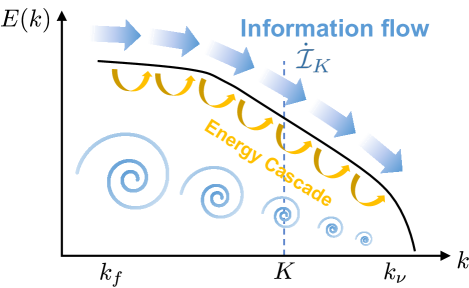
Figure 2: Schematic of information flow in the energy cascade.

V.2 Derivation of the main result

The derivation of the main result is based on the second law of information thermodynamics for bipartite systems [54]. Below, we first formulate the second law of thermodynamics [Ineq. (38)] and then derive the second law of information thermodynamics [Ineqs. (42) and (43)]. Finally, from the inequalities (42) and (43), we derive the main result.

V.2.1 Formulation of the second law of stochastic thermodynamics

First, we formulate the standard second law of thermodynamics. From a thermodynamic point of view, the fluctuating Navier–Stokes equation (5) and (6) consists of two parts: system and thermal environment [55]. Here, by system, we mean the independent Fourier modes $\{\hat{\bm{u}},\hat{\bm{u}}^{*}\}$, and by thermal environment, we mean the fast degrees of freedom associated with the microscopic molecular motion, which induce the viscous damping and thermal noise. In this paper, we treat entropy as dimensionless by dividing it by the Boltzmann constant $k_{\mathrm{B}}$.

Let $S[\hat{\bm{u}},\hat{\bm{u}}^{*}]$ be the entropy of the system, identified with the Shannon entropy

$$S[\hat{\bm{u}},\hat{\bm{u}}^{*}]:=-\int d\hat{\bm{u}}d\hat{\bm{u}}^{*}p_{t}(\hat{\bm{u}},\hat{\bm{u}}^{*})\ln p_{t}(\hat{\bm{u}},\hat{\bm{u}}^{*}),$$ (27)

where $d\hat{\bm{u}}d\hat{\bm{u}}^{*}:=\prod_{{\bm{k}}\in\mathcal{K}^{+}}\prod_{c\in\{x,y,z\}}d\mathrm{Re}[\hat{u}^{c}_{\bm{k}}]d\mathrm{Im}[\hat{u}^{c}_{\bm{k}}]$. Here, we use the notation $S[\hat{\bm{u}},\hat{\bm{u}}^{*}]$ to indicate the relevant random variables $\hat{\bm{u}}$ and $\hat{\bm{u}}^{*}$ although $S[\hat{\bm{u}},\hat{\bm{u}}^{*}]$ is not a function of $\hat{\bm{u}}$ and $\hat{\bm{u}}^{*}$. The average rate of change of the system entropy is given by

$$\quad\dfrac{d}{dt}S[\hat{\bm{u}},\hat{\bm{u}}^{*}]$$

$$=-\dfrac{d}{dt}\int d\hat{\bm{u}}d\hat{\bm{u}}^{*}p_{t}(\hat{\bm{u}},\hat{\bm{u}}^{*})\ln p_{t}(\hat{\bm{u}},\hat{\bm{u}}^{*})$$

$$=-\int d\hat{\bm{u}}d\hat{\bm{u}}^{*}(\partial_{t}p_{t}(\hat{\bm{u}},\hat{\bm{u}}^{*}))\ln p_{t}(\hat{\bm{u}},\hat{\bm{u}}^{*})$$

$$\qquad-\int d\hat{\bm{u}}d\hat{\bm{u}}^{*}\partial_{t}p_{t}(\hat{\bm{u}},\hat{\bm{u}}^{*})$$

$$=\int d\hat{\bm{u}}d\hat{\bm{u}}^{*}\sum_{{\bm{k}}\in\mathcal{K}^{+}}\left[\dfrac{\partial}{\partial\hat{\bm{u}}_{\bm{k}}}\cdot{\bm{J}}_{\bm{k}}(\hat{\bm{u}},\hat{\bm{u}}^{*})+\dfrac{\partial}{\partial\hat{\bm{u}}^{*}_{\bm{k}}}\cdot{\bm{J}}^{*}_{\bm{k}}(\hat{\bm{u}},\hat{\bm{u}}^{*})\right]$$

$$\qquad\times\ln p_{t}(\hat{\bm{u}},\hat{\bm{u}}^{*})$$

$$=\sum_{{\bm{k}}\in\mathcal{K}^{+}}\dot{S}_{\bm{k}}[\hat{\bm{u}},\hat{\bm{u}}^{*}].$$ (28)

Here, in the third equality, we have used the Fokker–Planck equation (9) and the fact that $\int d\hat{\bm{u}}d\hat{\bm{u}}^{*}\partial_{t}p_{t}(\hat{\bm{u}},\hat{\bm{u}}^{*})=d_{t}\int d\hat{\bm{u}}d\hat{\bm{u}}^{*}p_{t}(\hat{\bm{u}},\hat{\bm{u}}^{*})=0$. In the last equality, we have introduced $\dot{S}_{\bm{k}}[\hat{\bm{u}},\hat{\bm{u}}^{*}]$, which is given by

$$\dot{S}_{\bm{k}}[\hat{\bm{u}},\hat{\bm{u}}^{*}] :=-\int d\hat{\bm{u}}d\hat{\bm{u}}^{*}\left[{\bm{J}}_{\bm{k}}(\hat{\bm{u}},\hat{\bm{u}}^{*})\cdot\dfrac{\partial}{\partial\hat{\bm{u}}_{\bm{k}}}\ln p_{t}(\hat{\bm{u}},\hat{\bm{u}}^{*})\right.$$

$$\quad\left.+{\bm{J}}^{*}_{\bm{k}}(\hat{\bm{u}},\hat{\bm{u}}^{*})\cdot\dfrac{\partial}{\partial\hat{\bm{u}}^{*}_{\bm{k}}}\ln p_{t}(\hat{\bm{u}},\hat{\bm{u}}^{*})\right],$$ (29)

where the over-dot denotes the rates of change of observables that are not a time derivative of a state function.

We identify the entropy change in the environment according to Sekimoto’s argument [55]. Since the model satisfies the fluctuation-dissipation relation of the second kind, the thermal environment is ensured to be always in equilibrium at temperature $T$. Then, by noting that $-\nu k^{2}\hat{\bm{u}}_{\bm{k}}+\sqrt{2\nu k^{2}k_{\mathrm{B}}T/\rho}\hat{\bm{\xi}}_{\bm{k}}$ can be interpreted as a force exerted by the environment on the system, the entropy change in the environment is identified as the work done by the system on the environment per unit time divided by $k_{\mathrm{B}}T$:

$$\dot{S}^{\mathrm{env}} =\sum_{{\bm{k}}}\dfrac{\rho V}{2k_{\mathrm{B}}T}\left\langle\hat{\bm{u}}^{*}_{\bm{k}}\circ\left[\nu k^{2}\hat{\bm{u}}_{\bm{k}}-\sqrt{\dfrac{2\nu k^{2}k_{\mathrm{B}}T}{\rho}}\hat{\bm{\xi}}_{\bm{k}}\right]+\mathrm{c.c.}\right\rangle$$

$$=\sum_{{\bm{k}}\in\mathcal{K}^{+}}\dot{S}^{\mathrm{env}}_{\bm{k}},$$ (30)

where $\mathrm{c.c.}$ denotes the complex conjugate term and $\dot{S}^{\mathrm{env}}_{\bm{k}}$ denotes the entropy change in the environment associated with a wave vector ${\bm{k}}\in\mathcal{K}^{+}$,

$$\dot{S}^{\mathrm{env}}_{\bm{k}} :=\dfrac{\rho V}{k_{\mathrm{B}}T}\left\langle\hat{\bm{u}}^{*}_{\bm{k}}\circ\left[\nu k^{2}\hat{\bm{u}}_{\bm{k}}-\sqrt{\dfrac{2\nu k^{2}k_{\mathrm{B}}T}{\rho}}\hat{\bm{\xi}}_{\bm{k}}\right]+\mathrm{c.c.}\right\rangle.$$ (31)

Here, the symbol “$\circ$” denotes the multiplication in the sense of Stratonovich [50]. We remark that this identification is consistent with the local detailed balance (see Appendix C).

The total entropy production rate, which we denote by $\dot{\sigma}$, is identified as the sum of the average rate of change of the system entropy (28) and the entropy change in the environment (30):

$$\dot{\sigma} :=\dfrac{d}{dt}S[\hat{\bm{u}},\hat{\bm{u}}^{*}]+\dot{S}^{\mathrm{env}}$$

$$=\sum_{{\bm{k}}\in\mathcal{K}^{+}}\left(\dot{S}_{\bm{k}}[\hat{\bm{u}},\hat{\bm{u}}^{*}]+\dot{S}^{\mathrm{env}}_{\bm{k}}\right).$$ (32)

We now show that $\dot{\sigma}\geq 0$, which is a manifestation of the second law of thermodynamics and is sometimes called the second law of stochastic thermodynamics [49]. To this end, it is convenient to decompose the probability current (10) into two parts: ${\bm{J}}_{\bm{k}}(\hat{\bm{u}},\hat{\bm{u}}^{*})={\bm{J}}^{\mathrm{ir}}_{\bm{k}}(\hat{\bm{u}},\hat{\bm{u}}^{*})+{\bm{J}}^{\mathrm{rev}}_{\bm{k}}(\hat{\bm{u}},\hat{\bm{u}}^{*})$, where ${\bm{J}}^{\mathrm{ir}}_{\bm{k}}(\hat{\bm{u}},\hat{\bm{u}}^{*})$ denotes the irreversible probability current, defined by

$${\bm{J}}^{\mathrm{ir}}_{\bm{k}}(\hat{\bm{u}},\hat{\bm{u}}^{*}) :=\dfrac{1}{2}\left[{\bm{J}}_{\bm{k}}(\hat{\bm{u}},\hat{\bm{u}}^{*})-{\bm{J}}_{\bm{k}}(-\hat{\bm{u}},-\hat{\bm{u}}^{*})\right]$$

$$=-\nu k^{2}\hat{\bm{u}}_{\bm{k}}p_{t}(\hat{\bm{u}},\hat{\bm{u}}^{*})$$

$$\quad-\dfrac{1}{V}\dfrac{\nu k^{2}k_{\mathrm{B}}T}{\rho}\left(\mathsf{I}-\dfrac{{\bm{k}}{\bm{k}}}{k^{2}}\right)\cdot\dfrac{\partial}{\partial\hat{\bm{u}}^{*}_{\bm{k}}}p_{t}(\hat{\bm{u}},\hat{\bm{u}}^{*}),$$ (33)

and ${\bm{J}}^{\mathrm{rev}}_{\bm{k}}(\hat{\bm{u}},\hat{\bm{u}}^{*})$ denotes the reversible probability current, defined by

$${\bm{J}}^{\mathrm{rev}}_{\bm{k}}(\hat{\bm{u}},\hat{\bm{u}}^{*}) :=\dfrac{1}{2}[{\bm{J}}_{\bm{k}}(\hat{\bm{u}},\hat{\bm{u}}^{*})+{\bm{J}}_{\bm{k}}(-\hat{\bm{u}},-\hat{\bm{u}}^{*})]$$

$$=\left({\bm{B}}_{\bm{k}}(\hat{\bm{u}},\hat{\bm{u}}^{*})+\hat{\bm{f}}_{\bm{k}}\right)p_{t}(\hat{\bm{u}},\hat{\bm{u}}^{*}).$$ (34)

We then rewrite the average rate of change of the system entropy (28) as

$$\dfrac{d}{dt}S[\hat{\bm{u}},\hat{\bm{u}}^{*}] =-\sum_{{\bm{k}}\in\mathcal{K}^{+}}\int d\hat{\bm{u}}d\hat{\bm{u}}^{*}\left[{\bm{J}}_{\bm{k}}(\hat{\bm{u}},\hat{\bm{u}}^{*})\cdot\dfrac{\partial}{\partial\hat{\bm{u}}_{\bm{k}}}\ln p_{t}(\hat{\bm{u}},\hat{\bm{u}}^{*})+\mathrm{c.c.}\right]$$

$$=\sum_{{\bm{k}}\in\mathcal{K}^{+}}\dfrac{\rho V}{\nu k^{2}k_{\mathrm{B}}T}\int d\hat{\bm{u}}d\hat{\bm{u}}^{*}\left[\dfrac{{\bm{J}}^{\mathrm{ir}}_{\bm{k}}(\hat{\bm{u}},\hat{\bm{u}}^{*})}{p_{t}(\hat{\bm{u}},\hat{\bm{u}}^{*})}\cdot\left\{-\dfrac{1}{V}\dfrac{\nu k^{2}k_{\mathrm{B}}T}{\rho}\left(\mathsf{I}-\dfrac{{\bm{k}}{\bm{k}}}{k^{2}}\right)\cdot\dfrac{\partial}{\partial\hat{\bm{u}}_{\bm{k}}}p_{t}(\hat{\bm{u}},\hat{\bm{u}}^{*})\right\}+\mathrm{c.c.}\right],$$ (35)

where we have used the fact that

$$\dfrac{\partial}{\partial\hat{\bm{u}}_{\bm{k}}}\cdot\dfrac{{\bm{J}}^{\mathrm{rev}}_{\bm{k}}(\hat{\bm{u}},\hat{\bm{u}}^{*})}{p_{t}(\hat{\bm{u}},\hat{\bm{u}}^{*})}+\dfrac{\partial}{\partial\hat{\bm{u}}^{*}_{\bm{k}}}\cdot\dfrac{{\bm{J}}^{\mathrm{rev}*}_{\bm{k}}(\hat{\bm{u}},\hat{\bm{u}}^{*})}{p_{t}(\hat{\bm{u}},\hat{\bm{u}}^{*})}=-2i{\bm{k}}\cdot\hat{\bm{u}}_{\bm{0}}+2i{\bm{k}}\cdot\hat{\bm{u}}_{\bm{0}}=0$$ (36)

and that ${\bm{J}}^{\mathrm{ir}}_{\bm{k}}(\hat{\bm{u}},\hat{\bm{u}}^{*})$ is orthogonal to ${\bm{k}}$, i.e., ${\bm{J}}^{\mathrm{ir}}_{\bm{k}}(\hat{\bm{u}},\hat{\bm{u}}^{*})\cdot(\mathsf{I}-{\bm{k}}{\bm{k}}/k^{2})={\bm{J}}^{\mathrm{ir}}_{\bm{k}}(\hat{\bm{u}},\hat{\bm{u}}^{*})$. We also rewrite the entropy change in the environment (30) as

$$\dot{S}^{\mathrm{env}} :=\sum_{{\bm{k}}\in\mathcal{K}^{+}}\dfrac{\rho V}{k_{\mathrm{B}}T}\left\langle\hat{\bm{u}}^{*}_{\bm{k}}\circ\left[\nu k^{2}\hat{\bm{u}}_{\bm{k}}-\sqrt{\dfrac{2\nu k^{2}k_{\mathrm{B}}T}{\rho}}\hat{\bm{\xi}}_{\bm{k}}\right]+\mathrm{c.c.}\right\rangle$$

$$=\sum_{{\bm{k}}\in\mathcal{K}^{+}}\dfrac{\rho V}{k_{\mathrm{B}}T}\left\langle\hat{\bm{u}}^{*}_{\bm{k}}\cdot\left[\nu k^{2}\hat{\bm{u}}_{\bm{k}}-\sqrt{\dfrac{2\nu k^{2}k_{\mathrm{B}}T}{\rho}}\hat{\bm{\xi}}_{\bm{k}}\right]-\dfrac{1}{2}\dfrac{\partial}{\partial\hat{\bm{u}}^{*}_{\bm{k}}}\hat{\bm{u}}^{*}_{\bm{k}}:\left(\mathsf{I}-\dfrac{{\bm{k}}{\bm{k}}}{k^{2}}\right)\dfrac{2\nu k^{2}k_{\mathrm{B}}T}{\rho V}+\mathrm{c.c.}\right\rangle$$

$$=\sum_{{\bm{k}}\in\mathcal{K}^{+}}\dfrac{\rho V}{\nu k^{2}k_{\mathrm{B}}T}\int d\hat{\bm{u}}d\hat{\bm{u}}^{*}\left[\dfrac{-\nu k^{2}\hat{\bm{u}}^{*}_{\bm{k}}p_{t}(\hat{\bm{u}},\hat{\bm{u}}^{*})}{p_{t}(\hat{\bm{u}},\hat{\bm{u}}^{*})}\cdot{\bm{J}}^{\mathrm{ir}}_{\bm{k}}(\hat{\bm{u}},\hat{\bm{u}}^{*})+\mathrm{c.c.}\right].$$ (37)

Here, in the second line, we have used the relation between the Stratonovich and the Ito integral [50], so that the inner product “$\cdot$” here should be interpreted as the multiplication in the sense of Ito. Then, by combining (35) and (37), we can confirm that the total entropy production rate is nonnegative:

$$\dot{\sigma} =\sum_{{\bm{k}}\in\mathcal{K}^{+}}\left(\dot{S}_{\bm{k}}[\hat{\bm{u}},\hat{\bm{u}}^{*}]+\dot{S}^{\mathrm{env}}_{\bm{k}}\right)$$

$$=\sum_{{\bm{k}}\in\mathcal{K}^{+}}\int d\hat{\bm{u}}d\hat{\bm{u}}^{*}\dfrac{2\rho V}{\nu k^{2}k_{\mathrm{B}}T}\dfrac{|{\bm{J}}^{\mathrm{ir}}_{\bm{k}}(\hat{\bm{u}},\hat{\bm{u}}^{*})|^{2}}{p_{t}(\hat{\bm{u}},\hat{\bm{u}}^{*})}\geq 0.$$ (38)

V.2.2 Derivation of the second law of information thermodynamics

Now, we derive the second law of information thermodynamics. Let $\dot{\sigma}_{\bm{k}}:=\dot{S}_{\bm{k}}[\hat{\bm{u}},\hat{\bm{u}}^{*}]+\dot{S}^{\mathrm{env}}_{\bm{k}}$ be the partial entropy production rate [56] associated with a wave vector ${\bm{k}}\in\mathcal{K}^{+}$, so that $\dot{\sigma}=\sum_{{\bm{k}}\in\mathcal{K}^{+}}\dot{\sigma}_{\bm{k}}$. As is clear from the expression (38), $\dot{\sigma}_{\bm{k}}$ is also nonnegative for each wave vector ${\bm{k}}$:

$$\dot{\sigma}_{\bm{k}}=\int d\hat{\bm{u}}d\hat{\bm{u}}^{*}\dfrac{2\rho V}{\nu k^{2}k_{\mathrm{B}}T}\dfrac{|{\bm{J}}^{\mathrm{ir}}_{\bm{k}}(\hat{\bm{u}},\hat{\bm{u}}^{*})|^{2}}{p_{t}(\hat{\bm{u}},\hat{\bm{u}}^{*})}\geq 0.$$ (39)

From this relation, we can derive the second law of information thermodynamics for the two sets of Fourier modes ${\bm{U}}^{<}_{K}$ and ${\bm{U}}^{>}_{K}$. We first note that the information flow $\dot{I}^{<}_{K}$ associated with the large-scale modes ${\bm{U}}^{<}_{K}$ can be rewritten as

$$\dot{I}^{<}_{K} :=\lim_{dt\rightarrow 0^{+}}\dfrac{I[{\bm{U}}^{<}_{K}(t+dt):{\bm{U}}^{>}_{K}(t)]-I[{\bm{U}}^{<}_{K}(t):{\bm{U}}^{>}_{K}(t)]}{dt}$$

$$=\sum_{{\bm{k}}\in\mathcal{K}^{+},k\leq K}\int d\hat{\bm{u}}d\hat{\bm{u}}^{*}\left[{\bm{J}}_{\bm{k}}(\hat{\bm{u}},\hat{\bm{u}}^{*})\cdot\dfrac{\partial}{\partial\hat{\bm{u}}_{\bm{k}}}\ln\dfrac{p_{t}({\bm{U}}^{<}_{K},{\bm{U}}^{>}_{K})}{p^{<}_{t}({\bm{U}}^{<}_{K})p^{>}_{t}({\bm{U}}^{>}_{K})}+{\bm{J}}^{*}_{\bm{k}}(\hat{\bm{u}},\hat{\bm{u}}^{*})\cdot\dfrac{\partial}{\partial\hat{\bm{u}}^{*}_{\bm{k}}}\ln\dfrac{p_{t}({\bm{U}}^{<}_{K},{\bm{U}}^{>}_{K})}{p^{<}_{t}({\bm{U}}^{<}_{K})p^{>}_{t}({\bm{U}}^{>}_{K})}\right].$$ (40)

For the derivation, see Appendix B. By using this relation, we obtain

$$\dot{I}^{<}_{K} =-\sum_{{\bm{k}}\in\mathcal{K}^{+},k\leq K}\int d\hat{\bm{u}}d\hat{\bm{u}}^{*}\left[{\bm{J}}_{\bm{k}}(\hat{\bm{u}},\hat{\bm{u}}^{*})\cdot\dfrac{\partial}{\partial\hat{\bm{u}}_{\bm{k}}}\ln p^{<}_{t}({\bm{U}}^{<}_{K})+{\bm{J}}^{*}_{\bm{k}}(\hat{\bm{u}},\hat{\bm{u}}^{*})\cdot\dfrac{\partial}{\partial\hat{\bm{u}}^{*}_{\bm{k}}}\ln p^{<}_{t}({\bm{U}}^{<}_{K})\right]$$

$$\quad+\sum_{{\bm{k}}\in\mathcal{K}^{+},k\leq K}\int d\hat{\bm{u}}d\hat{\bm{u}}^{*}\left[{\bm{J}}_{\bm{k}}(\hat{\bm{u}},\hat{\bm{u}}^{*})\cdot\dfrac{\partial}{\partial\hat{\bm{u}}_{\bm{k}}}\ln p_{t}(\hat{\bm{u}},\hat{\bm{u}}^{*})+{\bm{J}}^{*}_{\bm{k}}(\hat{\bm{u}},\hat{\bm{u}}^{*})\cdot\dfrac{\partial}{\partial\hat{\bm{u}}^{*}_{\bm{k}}}\ln p_{t}(\hat{\bm{u}},\hat{\bm{u}}^{*})\right]$$

$$=\dfrac{d}{dt}S[{\bm{U}}^{<}_{K}]-\sum_{{\bm{k}}\in\mathcal{K}^{+},k\leq K}\dot{S}_{\bm{k}}[\hat{\bm{u}},\hat{\bm{u}}^{*}],$$ (41)

where $S[{\bm{U}}^{<}_{K}]:=-\int d{\bm{U}}^{<}_{K}p^{<}_{t}({\bm{U}}^{<}_{K})\ln p^{<}_{t}({\bm{U}}^{<}_{K})$ denotes the Shannon entropy of the large-scale modes ${\bm{U}}^{<}_{K}$. Then, by summing (39) over all ${\bm{k}}$ that satisfies ${\bm{k}}\in\mathcal{K}^{+}$ and $k\leq K$ and by using (41), we obtain the second law of information thermodynamics for the large-scale modes:

$$\sum_{{\bm{k}}\in\mathcal{K}^{+},k\leq K}\dot{\sigma}_{\bm{k}}=\dfrac{d}{dt}S[{\bm{U}}^{<}_{K}]+\dot{S}^{<}_{\mathrm{env}}-\dot{I}^{<}_{K}\geq 0,$$ (42)

where $\dot{S}^{<}_{\mathrm{env}}:=\sum_{{\bm{k}}\in\mathcal{K}^{+},k\leq K}\dot{S}^{\mathrm{env}}_{\bm{k}}$ denotes the entropy change in the environment due to the large-scale modes. Similarly, we can obtain the second law of information thermodynamics for the small-scale modes:

$$\sum_{{\bm{k}}\in\mathcal{K}^{+},k>K}\dot{\sigma}_{\bm{k}}=\dfrac{d}{dt}S[{\bm{U}}^{>}_{K}]+\dot{S}^{>}_{\mathrm{env}}-\dot{I}^{>}_{K}\geq 0.$$ (43)

Note that the first two terms on the right-hand side of (42) and (43) can be interpreted as the total entropy production rate associated with the large-scale and small-scale modes, respectively. Then, (42) and (43) state that the total entropy production associated with each mode is not necessarily nonnegative but is bounded by the information flow. In particular, if ${\bm{U}}^{<}_{K}$ and ${\bm{U}}^{>}_{K}$ are statistically independent, then $\dot{I}^{<}_{K}=\dot{I}^{>}_{K}=0$ and the standard second law of thermodynamics holds for each mode. In contrast, if they are correlated, then the inequalities (42) and (43) give nontrivial bounds on the information flow in terms of the entropy production.

V.2.3 Derivation of the main result

We now derive the main results (25) and (26) from the second law of information thermodynamics (42) and (43). We assume that the system is in the steady state. Then, by noting that $\dot{\mathcal{I}}_{K}=\dot{I}^{>}_{K}=-\dot{I}^{<}_{K}$, (42) and (43) can be rewritten as

$$\dot{S}^{<}_{\mathrm{env}}+\dot{\mathcal{I}}_{K}\geq 0,$$ (44)

$$\dot{S}^{>}_{\mathrm{env}}-\dot{\mathcal{I}}_{K}\geq 0,$$ (45)

respectively. We set $K$ to be within the inertial range $k_{f}\ll K\ll k_{\nu}$. Then, $\dot{S}^{<}_{\mathrm{env}}$ can be expressed in terms of the energy flux (17) as

$$\dot{S}^{<}_{\mathrm{env}} =\sum_{{\bm{k}}\in\mathcal{K}^{+},k\leq K}\dfrac{\rho V}{k_{\mathrm{B}}T}$$

$$\quad\times\left\langle\hat{\bm{u}}^{*}_{\bm{k}}\circ\left[\nu k^{2}\hat{\bm{u}}_{\bm{k}}-\sqrt{\dfrac{2\nu k^{2}k_{\mathrm{B}}T}{\rho}}\hat{\bm{\xi}}_{\bm{k}}\right]+\mathrm{c.c.}\right\rangle$$

$$=\sum_{k\leq K}\dfrac{1}{2}\dfrac{\rho V}{k_{\mathrm{B}}T}$$

$$\quad\times\left\langle\hat{\bm{u}}^{*}_{\bm{k}}\circ\left[{\bm{B}}_{\bm{k}}(\hat{\bm{u}},\hat{\bm{u}}^{*})+\hat{\bm{f}}_{\bm{k}}-\partial_{t}\hat{\bm{u}}_{\bm{k}}\right]+\mathrm{c.c.}\right\rangle$$

$$=\dfrac{\rho V}{k_{\mathrm{B}}T}\left(\varepsilon-\Pi_{K}\right),$$ (46)

where we have used $\sum_{k\leq K}\langle\hat{\bm{f}}_{\bm{k}}\cdot\hat{\bm{u}}^{*}_{\bm{k}}+\hat{\bm{f}}^{*}_{\bm{k}}\cdot\hat{\bm{u}}_{\bm{k}}\rangle/2=\varepsilon$ for $K$ within the inertial range $k_{f}\ll K\ll k_{\nu}$ and $\langle\hat{\bm{u}}^{*}_{\bm{k}}\circ\partial_{t}\hat{\bm{u}}_{\bm{k}}+\hat{\bm{u}}_{\bm{k}}\circ\partial_{t}\hat{\bm{u}}^{*}_{\bm{k}}\rangle=d_{t}\langle|\hat{\bm{u}}_{\bm{k}}|^{2}\rangle=0$ in the steady state. Similarly, $\dot{S}^{>}_{\mathrm{env}}$ can be expressed as

$$\dot{S}^{>}_{\mathrm{env}} =\dfrac{\rho V}{k_{\mathrm{B}}T}\Pi_{K},$$ (47)

where we have used the property of the nonlinear term (12). By substituting these expressions into (44) and (45) and by noting that $\Pi_{K}\rightarrow\varepsilon$ as $K/k_{\nu}\rightarrow 0$, we arrive at the main result (25) and (26).

VI Numerical simulation

We here numerically illustrate the main result by estimating the information flow $\dot{\mathcal{I}}_{K}$. Since the estimation of the information flow for the fluctuating Navier–Stokes equation requires an enormous computational cost, we instead use a fluctuating shell model, which is a simplified caricature of the fluctuating Navier–Stokes equation in wave number space. Even for the fluctuating shell model, we can easily confirm that the main results (25) and (26) are valid. In the following, we first introduce the fluctuating shell model in Sec. VI.1. Next, we explain the setup of the numerical simulation in Sec. VI.2. The numerical simulation results are presented in Sec. VI.3.

VI.1 Model

We consider the Sabra shell model with thermal noise [57, 42, 43]. Let $u_{n}(t)\in\mathbb{C}$ be the “velocity” at time $t$ with the wave number $k_{n}=k_{0}2^{n}$ ($n=0,1,\cdots,N$). The time evolution of the complex shell variables $u:=\{u_{n}\}$ is given by the following Langevin equation:

$$\partial_{t}{u}_{n}=B_{n}(u,u^{*})-\nu k^{2}_{n}u_{n}+\sqrt{\dfrac{2\nu k^{2}_{n}k_{\mathrm{B}}T}{\rho}}\xi_{n}+f_{n}$$ (48)

with the scale-local nonlinear interactions given by

$$B_{n}(u,u^{*}) :=i\biggl{(}k_{n+1}u_{n+2}u^{*}_{n+1}$$

$$\quad-\dfrac{1}{2}k_{n}u_{n+1}u^{*}_{n-1}+\dfrac{1}{2}k_{n-1}u_{n-1}u_{n-2}\biggr{)},$$ (49)

where we set $u_{-1}=u_{-2}=u_{N+1}=u_{N+2}=0$. Here, $\nu>0$ represents the kinematic viscosity, $f_{n}\in\mathbb{C}$ denotes the external body force that acts only at large scales, i.e., $f_{n}=0$ for $n>n_{f}$, and $\xi_{n}\in\mathbb{C}$ is the zero-mean white Gaussian noise that satisfies $\langle\xi_{n}(t)\xi^{*}_{n^{\prime}}(t^{\prime})\rangle=2\delta_{nn^{\prime}}\delta(t-t^{\prime})$. The specific form of the thermal noise term satisfies the fluctuation-dissipation relation of the second kind, where $T$ denotes the absolute temperature, $k_{\mathrm{B}}$ the Boltzmann constant, and $\rho$ the mass “density”.

Although the shell model has a much simpler form than the Navier–Stokes equation, it exhibits rich temporal and multiscale statistics that are similar to those observed in real turbulent flow [58, 59]. In particular, the energy cascade property (18) is satisfied even for this model. Then, we can easily confirm that the main results (25) and (26) are valid:

$$\dot{\mathcal{I}}_{K} \geq 0,$$ (50)

$$\dfrac{\rho\varepsilon}{k_{\mathrm{B}}T} \geq\dot{\mathcal{I}}_{K},$$ (51)

for $K$ within the inertial range $k_{f}\ll K\ll k_{\nu}$, where $k_{f}:=k_{n_{f}}$ and $k_{\nu}\equiv\eta^{-1}:=\nu^{-3/4}\varepsilon^{1/4}$. Note that, in contrast to (26), the volume of the fluid $V$ does not appear in (51) because $\rho$ has units of mass in the shell model.

VI.2 Setup of the numerical simulation

Table 1: The largest shell number $N$, the achieved Reynolds number $\mathrm{Re}$, and the dimensionless temperature $\theta_{\eta}$ of the three different cases.

Case	$N$	$\mathrm{Re}$	$\theta_{\eta}$
I	$22$	$1.46\times 10^{6}$	$2.328\times 10^{-8}$
II	$19$	$9.25\times 10^{4}$	$2.328\times 10^{-8}$
III	$22$	$1.46\times 10^{6}$	$0$

To investigate the Reynolds number and temperature dependence of the information flow, we consider three different cases as listed in Table 1. In Case I, we set $N=22$ and $n_{f}=1$ to ensure that the external force acts only on the 0th and 1st shells of the total 23 shells. In choosing the parameter values, we note that the presence of thermal fluctuations introduces another dimensionless quantity $\theta_{\eta}:=k_{\mathrm{B}}T/\rho u^{2}_{\eta}$ in addition to the Reynolds number $\mathrm{Re}$. Here, $u_{\eta}:=(\varepsilon\nu)^{1/4}$ denotes the characteristic velocity at the Kolmogorov dissipation scale, and thus the dimensionless temperature $\theta_{\eta}$ is the ratio of the thermal energy to the kinetic energy at the Kolmogorov dissipation scale. Then, the values of the external force and the other parameters are chosen following Refs. [42, 43] so that the achieved Reynolds number $\mathrm{Re}$ and the dimensionless temperature $\theta_{\eta}$ are both comparable to the typical values in the atmospheric boundary layer, i.e., $\mathrm{Re}\sim 10^{6}$ and $\theta_{\eta}\sim 10^{-8}$. In Case II, we set $N=19$ so that the achieved Reynolds number is lowered to $\mathrm{Re}\sim 10^{5}$ while leaving the other parameter values unchanged. In Case III, we consider the standard deterministic case by setting $T=0$ ($\theta_{\eta}=0$) while leaving the other parameter values unchanged. In all three cases, we have used $N_{\mathrm{samp}}=3\times 10^{5}$ samples in the following averaging and estimation.

In the estimation of the mutual information, we first note that the naive binning approach is not feasible because it requires estimation of the $2(N+1)$-dimensional probability density $p_{t}({\bm{U}}^{<}_{K},{\bm{U}}^{>}_{K})$. Instead, we use the so-called Kraskov-Stögbauer-Grassberger (KSG) estimator [60, 61, 62], which has the advantage that it does not require estimation of the underlying probability density. The KSG estimator uses the distances to the $\kappa$-th nearest neighbors of the sample points in the data to detect the structures of the underlying probability distribution. While we set $\kappa=4$ here, following Ref. [60], essentially the same result can be obtained for other values of $\kappa$. Because the KSG estimator is based on the local uniformity assumption of the probability density, the estimated value approaches the true value as $N_{\mathrm{samp}}\rightarrow\infty$ when this assumption is satisfied. In the following, we denote by $\hat{I}^{(\kappa)}_{\mathrm{KSG}}[{\bm{U}}^{<}_{K}(t):{\bm{U}}^{>}_{K}(t)]$ the KSG estimator of the mutual information $I[{\bm{U}}^{<}_{K}(t):{\bm{U}}^{>}_{K}(t)]$.

The information flow $\dot{\mathcal{I}}_{K}$ can be estimated by using the KSG estimator. Note that this procedure requires high accuracy in the estimation of the mutual information because the information flow is defined through infinitesimal increments in the mutual information. Because it is not feasible to increase the number of samples, we instead take the approach of using the largest possible time increment $\Delta t$. That is, we define the estimated information flow $\hat{\dot{\mathcal{I}}}_{K}$ by

$$\hat{\dot{\mathcal{I}}}_{K}:=-\dfrac{\hat{I}^{(\kappa)}_{\mathrm{KSG}}[{\bm{U}}^{<}_{K}(t+\Delta t):{\bm{U}}^{>}_{K}(t)]-\hat{I}^{(\kappa)}_{\mathrm{KSG}}[{\bm{U}}^{<}_{K}(t):{\bm{U}}^{>}_{K}(t)]}{\Delta t}.$$ (52)

Because we are interested in $K$ within the inertial range, we choose $\Delta t$ such that it is smaller than the smallest time scale in the inertial range. Therefore, we set $\Delta t=0.1\tau_{\eta}$, where $\tau_{\eta}:=\eta/u_{\eta}$ denotes the typical time scale at the Kolmogorov dissipation scale. Note that $\Delta t$ is different from the time step $\delta t:=10^{-5}\tau_{\eta}$ used in solving (48) numerically.

Further details of the numerical simulation are given in Appendix D, including the details of the KSG estimator.

VI.3 Results

VI.3.1 Energy spectrum

Figure 3(a) shows the energy spectrum $E_{n}:=\langle|u_{n}|^{2}\rangle_{\mathrm{ss}}/2$ in the steady state. The achieved Reynolds numbers are $\mathrm{Re}\simeq 9.25\times 10^{4}$ for Case II and $1.46\times 10^{6}$ for Case I and III. In all three cases, we can see that the spectrum is consistent with the Kolmogorov spectrum in the inertial range, $E_{n}\propto k^{-2/3}_{n}$. In the dissipation range, the spectrum exhibits the stretched-exponential decay in Case III, while it exhibits the equipartition of energy $E_{n}=k_{\mathrm{B}}T/\rho$ ($E_{n}/u^{2}_{\eta}=\theta_{\eta}$ in the dimensionless form) in Case I and II. We also note that while the thermal fluctuation effects are negligible in the inertial range, they become relevant already at the length scale $k\eta\sim 10$, as pointed out in Ref. [42, 43].

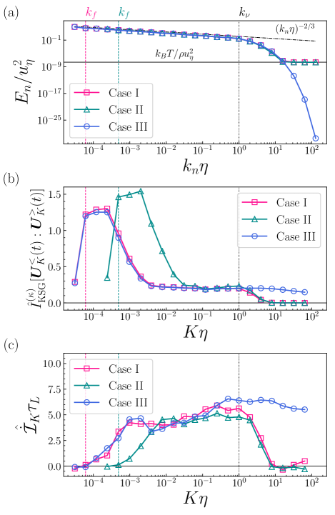
Figure 3: (a) Scale dependence of the energy spectrum $E_{n}=\langle|u_{n}|^{2}\rangle_{\mathrm{ss}}/2$. The dash-dotted line represents $\varepsilon^{2/3}k^{-2/3}_{n}$. The solid line represents the thermal equipartition value $k_{\mathrm{B}}T/\rho$. (b) Scale dependence of the estimated mutual information $\hat{I}^{(\kappa)}_{\mathrm{KSG}}[{\bm{U}}^{<}_{K}(t):{\bm{U}}^{>}_{K}(t)]$ with $\kappa=4$. The error bars are within the marker size. (c) Scale dependence of the estimated information flow $\hat{\dot{\mathcal{I}}}_{K}$. Note that it is plotted in units of the inverse of $\tau_{L}$. In all panels, the dotted and dashed lines represent the Kolmogorov dissipation scale $k_{\nu}=1/\eta$ and injection scale $k_{f}$, respectively.

VI.3.2 Mutual information

Figure 3(b) shows the scale dependence of the estimated mutual information $\hat{I}^{(\kappa)}_{\mathrm{KSG}}[{\bm{U}}^{<}_{K}(t):{\bm{U}}^{>}_{K}(t)]$. Its standard deviation is also estimated to be $\sim 10^{-3}$ by subsampling [62] (see Appendix D.3), which lies within the marker size. Notably, the mutual information is almost independent of $K$ in the inertial range. Furthermore, Fig. 3(b) implies that the mutual information is also independent of $\mathrm{Re}$ and $T$ in the inertial range. In other words, if we divide the total shell variables into the large-scale and small-scale modes at an arbitrary wave number $K$ within the inertial range, then the correlation between the large-scale and small-scale modes is not affected by $\mathrm{Re}$ and $T$. In the energy injection and dissipation scale range, however, the mutual information significantly depends on $\mathrm{Re}$ and $T$. In particular, the mutual information becomes zero in the dissipation range for Case I and II, while it remains finite for Case III. This is because the thermal fluctuation destroys the correlation, and the large-scale and small-scale modes become statistically independent.

VI.3.3 Information flow

In Fig. 3(c), we show the estimated information flow $\hat{\dot{\mathcal{I}}}_{K}$ in units of the inverse of the large-eddy turnover time $\tau_{L}:=1/k_{0}u_{\mathrm{rms}}$, where $u^{2}_{\mathrm{rms}}:=\sum^{N}_{n=0}\langle|u_{n}|^{2}\rangle_{\mathrm{ss}}$. We find that $\tau_{L}\simeq 181\tau_{\eta}$ for Case II, while $\tau_{L}\simeq 734\tau_{\eta}$ for Case I and III. From this figure, we can see that the information flow takes positive values for $K$ within the inertial range, consistent with the main result (25). Thus, information of large-scale turbulent fluctuations is indeed transferred to small scales.

For the second inequality (26), we note that the upper bound in units of $\tau^{-1}_{L}$ reads $(\rho\varepsilon/k_{\mathrm{B}}T)\tau_{L}\simeq 7.79\times 10^{9}$ for Case II and $3.15\times 10^{10}$ for Case I and III. Therefore, the inequality (26) is also satisfied, although it is a rather loose bound. This result can be reinterpreted using the concept of information-thermodynamic efficiency [54], defined by

$$\eta_{\mathrm{eff}}:=\dfrac{\dot{\mathcal{I}}_{K}}{\dot{S}^{>}_{\mathrm{env}}}=\dfrac{\dot{\mathcal{I}}_{K}}{\rho\varepsilon/k_{\mathrm{B}}T}.$$ (53)

From the main result (25) and the second law of information thermodynamics in the steady state (45), it immediately follows that $0\leq\eta_{\mathrm{eff}}\leq 1$. This efficiency quantifies how efficiently the small-scale modes ${\bm{U}}^{>}_{K}$ gain information about the large-scale modes ${\bm{U}}^{<}_{K}$ relative to the energy dissipation or thermodynamic cost. Then, the previous result states that $\eta_{\mathrm{eff}}\ll 1$, which suggests that the small-scale eddies acquire information about the large-scale eddies at a relatively high thermodynamic cost. This property is in contrast to other typical information processing systems such as Maxwell’s demon [54, 35, 53] and thus characterizes turbulence dynamics.

Furthermore, Fig. 3(c) suggests that the information flow may be scaled as

$$\dot{\mathcal{I}}_{K}\sim\dfrac{C}{\tau_{L}}$$ (54)

in the inertial range, where $C$ is a dimensionless constant that is almost independent of $\mathrm{Re}$, $K$, and $T$. By noting that $\tau_{L}$ can be interpreted as the characteristic time scale for the largest eddies to be stretched into smaller eddies, this result implies that the information of large-scale eddies is transferred to small scales by the energy cascade process with nearly constant intensity. This result also implies that, although thermal fluctuations are crucial in deriving the main results (25) and (26), the information flow itself is mainly governed by the large-scale dynamics rather than by the thermal fluctuations.

VII Concluding remarks

In summary, we have proved that, in fully developed three-dimensional fluid turbulence, information of turbulent fluctuations is transferred from large to small scales along with the energy cascade. Our main results (25) and (26) are a direct consequence of the second law of information thermodynamics, and thus they are exact and universal relations, independent of the details of the flow under consideration. Furthermore, our numerical simulation using a shell model suggests that the intensity of the information flow is nearly constant in the inertial range and that the rate of information transfer is characterized by the large-eddy turnover time [Eq. (54)]. This observation states that the information of large-scale turbulent fluctuations is transferred to small scales by the energy cascade process with nearly constant intensity. Thus, our results challenge the conventional intuitive picture that the universal statistical properties emerge at small scales because information about the details of the large scales is lost in the cascade process. Moreover, we have found that the information-thermodynamic efficiency is quite low compared to other typical information processing systems such as Maxwell’s demon. This implies that transferring information from large to small scales involves enormous thermodynamic costs, indicating the poor performance of turbulence as an information processing system.

We now provide some technical remarks on the estimation of the information flow. Although the KSG estimator used here is asymptotically unbiased for $N_{\mathrm{samp}}\rightarrow\infty$, there are a sample-size-dependent bias and a $\kappa$-dependent bias for a finite $N_{\mathrm{samp}}$ in general [62]. In our case, we have found that the magnitude of $\hat{I}^{(\kappa)}_{\mathrm{KSG}}[{\bm{U}}^{<}_{K}:{\bm{U}}^{>}_{K}]$ depends on $\kappa$. This may be because the probability distribution $p_{t}({\bm{U}}^{<}_{K},{\bm{U}}^{>}_{K})$ is skewed and has heavy tails, thus violating the local uniformity condition [62]. Nevertheless, we have confirmed that the sign of $\hat{\dot{\mathcal{I}}}_{K}$ does not depend on the choice of $\kappa$. See Appendix D for more details on these subtle points. It should also be noted that the number of samples $N_{\mathrm{samp}}$ used here is not sufficient for high accurate estimation of the information flow because the standard deviation of the estimated mutual information is comparable to its increment. In other words, if we naively estimate the error bar of the information flow $\hat{\dot{\mathcal{I}}}_{K}$ by using the estimated standard deviation of the mutual information, it is of the same order as $\hat{\dot{\mathcal{I}}}_{K}$ itself. It is therefore desirable to perform the numerical calculations with higher accuracy while taking the bias into account.

Our study opens several possible directions for future research. The first direction concerns the origin of the universality of turbulent fluctuations at small scales. As we have mentioned above, our result here is somewhat contrary to the common intuitive picture of how universality emerges at small scales. Then, it seems natural to ask how the universality emerges at small scales under the influence of the information flow from large scales. We conjecture that the coexistence of the universality and information flow can be explained by the stepwise “information cascade” process where “irrelevant information” is “deamplified” as the cascade develops. The role of various energy cascade mechanisms [10, 63] in this process would be an interesting question to be investigated. Note that this cascade picture is analogous to that proposed by Wilson in the context of the critical phenomena [64]. The second direction concerns the intermittency. Since there is an information flow of turbulent fluctuations from large to small scales, the small-scale intermittency must be affected by the information flow. Indeed, the intermittency implies that the turbulent fluctuations grow in each cascade step and thus “remember” the large scales [4, 8, 7]. Therefore, we guess that there are universal relations between the intermittency and the information flow that restrict the possible values of the structure function exponent $\zeta_{p}$. Finally, because turbulent cascade is a ubiquitous phenomenon found in quantum fluids [65, 66, 67, 68], supercritical fluids near a critical point [69], elastic bodies [70, 71], and even spin systems [72, 73, 74], it would be interesting research direction to investigate the nature of the information flow in these various systems. We hope that our work opens up a new research area, “information hydrodynamics,” which would provide a theoretical framework to elucidate and control the dynamics of complicated hydrodynamic phenomena.

Appendix A Detailed calculation of the Fourier transform of the fluctuating Navier–Stokes equation

By applying the Fourier transform to the fluctuating Navier–Stokes equation (1), we obtain

$$\partial_{t}\hat{\bm{u}}_{\bm{k}} =-i{\bm{k}}\cdot\sum_{{\bm{p}}+{\bm{q}}={\bm{k}}}\hat{\bm{u}}_{\bm{p}}\hat{\bm{u}}_{\bm{q}}-i{\bm{k}}\hat{p}_{\bm{k}}-\nu k^{2}\hat{\bm{u}}_{\bm{k}}+\hat{\bm{f}}_{\bm{k}}+i{\bm{k}}\cdot\hat{\mathsf{s}}_{\bm{k}}.$$ (55)

Here, $\hat{\mathsf{s}}_{\bm{k}}$ denotes the zero-mean white Gaussian noise that satisfies

$$\quad\langle\hat{\mathsf{s}}^{ab}_{\bm{k}}(t)\hat{\mathsf{s}}^{cd*}_{{\bm{k}}^{\prime}}(t^{\prime})\rangle$$

$$=\dfrac{1}{V}\dfrac{2\nu k_{\mathrm{B}}T}{\rho}\left(\delta^{ac}\delta^{bd}+\delta^{ad}\delta^{bc}-\dfrac{2}{3}\delta^{ab}\delta^{cd}\right)\delta_{{\bm{k}},{\bm{k}}^{\prime}}\delta(t-t^{\prime}).$$ (56)

We define $\hat{\bm{\xi}}_{\bm{k}}$ by $\sqrt{2\nu k^{2}k_{\mathrm{B}}T/\rho}\hat{\bm{\xi}}_{\bm{k}}=i{\bm{k}}\cdot\hat{\mathsf{s}}_{\bm{k}}$, which satisfies

$$\langle\hat{\xi}^{a}_{\bm{k}}(t)\hat{\xi}^{b*}_{{\bm{k}}^{\prime}}(t^{\prime})\rangle=\dfrac{1}{V}\left(\delta^{ab}+\dfrac{1}{3}\dfrac{k^{a}k^{b}}{k^{2}}\right)\delta_{{\bm{k}},{\bm{k}}^{\prime}}\delta(t-t^{\prime}).$$ (57)

We decompose $\hat{\bm{\xi}}_{\bm{k}}$ into components parallel and perpendicular to ${\bm{k}}$: $\hat{\bm{\xi}}_{\bm{k}}=\hat{\bm{\xi}}^{\parallel}_{\bm{k}}+\hat{\bm{\xi}}^{\perp}_{\bm{k}}$, where $\hat{\bm{\xi}}^{\perp}_{\bm{k}}=(\mathsf{1}-{\bm{k}}{\bm{k}}/k^{2})\cdot\hat{\bm{\xi}}_{\bm{k}}$, which satisfies

$$\langle\hat{\xi}^{\perp a}_{\bm{k}}(t)\hat{\xi}^{\perp b*}_{{\bm{k}}^{\prime}}(t^{\prime})\rangle=\dfrac{1}{V}\left(\delta^{ab}-\dfrac{k^{a}k^{b}}{k^{2}}\right)\delta_{{\bm{k}},{\bm{k}}^{\prime}}\delta(t-t^{\prime}).$$ (58)

Then, by multiplying ${\bm{k}}$ to (55) and by noting that ${\bm{k}}\cdot\hat{\bm{u}}_{\bm{k}}={\bm{k}}\cdot\hat{\bm{f}}_{\bm{k}}=0$, we obtain

$$-i\hat{p}_{\bm{k}}+\sqrt{\dfrac{2\nu k_{\mathrm{B}}T}{\rho}}\hat{\xi}^{\parallel}_{\bm{k}}=i\dfrac{{\bm{k}}{\bm{k}}}{k^{2}}:\sum_{{\bm{p}}+{\bm{q}}={\bm{k}}}\hat{\bm{u}}_{\bm{p}}\hat{\bm{u}}_{\bm{q}},$$ (59)

where $\hat{\xi}^{\parallel}_{\bm{k}}=({\bm{k}}/k)\cdot\hat{\bm{\xi}}^{\parallel}_{\bm{k}}$. By substituting this relation into (55), we arrive at (5). Note that, in (5), $\hat{\bm{\xi}}^{\perp}_{\bm{k}}$ is rewritten as $\hat{\bm{\xi}}_{\bm{k}}$ for notational simplicity.

Appendix B Derivation of Eqs. (23) and (40)

We first derive the expression (40). Let $p(\tilde{\bm{U}}^{<}_{K},t+h;{\bm{U}}^{>}_{K},t)$ be the two-point probability density with $\tilde{\bm{U}}^{<}_{K}={\bm{U}}^{<}_{K}(t+h)$ and ${\bm{U}}^{>}_{K}={\bm{U}}^{>}_{K}(t)$. When $h=0$, it corresponds to the joint probability density at the same time $t$: $p({\bm{U}}^{<}_{K},t;{\bm{U}}^{>}_{K},t)=p_{t}({\bm{U}}^{<}_{K},{\bm{U}}^{>}_{K})$. Then, from the definition of the information flow (21), we find that

$$\dot{I}^{<}_{K} :=\lim_{dt\rightarrow 0^{+}}\dfrac{I[{\bm{U}}^{<}_{K}(t+dt):{\bm{U}}^{>}_{K}(t)]-I[{\bm{U}}^{<}_{K}(t):{\bm{U}}^{>}_{K}(t)]}{dt}$$

$$=\lim_{h\rightarrow 0^{+}}\dfrac{1}{h}\left(\int d\tilde{\bm{U}}^{<}_{K}d{\bm{U}}^{>}_{K}p(\tilde{\bm{U}}^{<}_{K},t+h;{\bm{U}}^{>}_{K},t)\ln\dfrac{p(\tilde{\bm{U}}^{<}_{K},t+h;{\bm{U}}^{>}_{K},t)}{p^{<}_{t+h}(\tilde{\bm{U}}^{<}_{K})p^{>}_{t}({\bm{U}}^{>}_{K})}-\int d{\bm{U}}^{<}_{K}d{\bm{U}}^{>}_{K}p_{t}({\bm{U}}^{<}_{K},{\bm{U}}^{>}_{K})\ln\dfrac{p_{t}({\bm{U}}^{<}_{K},{\bm{U}}^{>}_{K})}{p^{<}_{t}({\bm{U}}^{<}_{K})p^{>}_{t}({\bm{U}}^{>}_{K})}\right)$$

$$=\int d\tilde{\bm{U}}^{<}_{K}d\tilde{\bm{U}}^{>}_{K}d{\bm{U}}^{<}_{K}d{\bm{U}}^{>}_{K}\left.\dfrac{\partial}{\partial h}p(\tilde{\bm{U}}^{<}_{K},\tilde{\bm{U}}^{>}_{K},t+h|{\bm{U}}^{<}_{K},{\bm{U}}^{>}_{K},t)\right|_{h=0}p_{t}({\bm{U}}^{<}_{K},{\bm{U}}^{>}_{K})\ln\dfrac{p_{t}(\tilde{\bm{U}}^{<}_{K},{\bm{U}}^{>}_{K})}{p^{<}_{t}(\tilde{\bm{U}}^{<}_{K})p^{>}_{t}({\bm{U}}^{>}_{K})},$$ (60)

where we have used $\int d\tilde{\bm{U}}^{<}_{K}d{\bm{U}}^{>}_{K}\frac{\partial}{\partial h}p(\tilde{\bm{U}}^{<}_{K},t+h;{\bm{U}}^{>}_{K},t)=\frac{\partial}{\partial h}\int d\tilde{\bm{U}}^{<}_{K}d{\bm{U}}^{>}_{K}p(\tilde{\bm{U}}^{<}_{K},t+h;{\bm{U}}^{>}_{K},t)=0$ and

$$p(\tilde{\bm{U}}^{<}_{K},t+h;{\bm{U}}^{>}_{K},t) =\int d\tilde{\bm{U}}^{>}_{K}d{\bm{U}}^{<}_{K}p(\tilde{\bm{U}}^{<}_{K},\tilde{\bm{U}}^{>}_{K},t+h;{\bm{U}}^{<}_{K},{\bm{U}}^{>}_{K},t)$$

$$=\int d\tilde{\bm{U}}^{>}_{K}d{\bm{U}}^{<}_{K}p(\tilde{\bm{U}}^{<}_{K},\tilde{\bm{U}}^{>}_{K},t+h|{\bm{U}}^{<}_{K},{\bm{U}}^{>}_{K},t)p_{t}({\bm{U}}^{<}_{K},{\bm{U}}^{>}_{K}),$$ (61)

where $p(\tilde{\bm{U}}^{<}_{K},\tilde{\bm{U}}^{>}_{K},t+h|{\bm{U}}^{<}_{K},{\bm{U}}^{>}_{K},t)=p(\tilde{\bm{U}}^{<}_{K},\tilde{\bm{U}}^{>}_{K},t+h;{\bm{U}}^{<}_{K},{\bm{U}}^{>}_{K},t)/p_{t}({\bm{U}}^{<}_{K},{\bm{U}}^{>}_{K})$ denotes the conditional probability density. By noting that $p(\tilde{\bm{U}}^{<}_{K},\tilde{\bm{U}}^{>}_{K},t+h|{\bm{U}}^{<}_{K},{\bm{U}}^{>}_{K},t)$ obeys the Fokker–Planck equation (9) and that $p(\tilde{\bm{U}}^{<}_{K},\tilde{\bm{U}}^{>}_{K},t|{\bm{U}}^{<}_{K},{\bm{U}}^{>}_{K},t)=\delta(\tilde{\bm{U}}^{<}_{K}-{\bm{U}}^{<}_{K})\delta(\tilde{\bm{U}}^{>}_{K}-{\bm{U}}^{>}_{K})$, we arrive at (40):

$$\dot{I}^{<}_{K} =\int d{\bm{U}}^{<}_{K}d{\bm{U}}^{>}_{K}\sum_{{\bm{k}}\in\mathcal{K}^{+},k\leq K}\left[-\dfrac{\partial}{\partial\hat{\bm{u}}_{\bm{k}}}\cdot{\bm{J}}_{\bm{k}}(\hat{\bm{u}},\hat{\bm{u}}^{*})-\dfrac{\partial}{\partial\hat{\bm{u}}^{*}_{\bm{k}}}\cdot{\bm{J}}^{*}_{\bm{k}}(\hat{\bm{u}},\hat{\bm{u}}^{*})\right]\ln\dfrac{p_{t}({\bm{U}}^{<}_{K},{\bm{U}}^{>}_{K})}{p^{<}_{t}({\bm{U}}^{<}_{K})p^{>}_{t}({\bm{U}}^{>}_{K})}$$

$$=\sum_{{\bm{k}}\in\mathcal{K}^{+},k\leq K}\int d\hat{\bm{u}}d\hat{\bm{u}}^{*}\left[{\bm{J}}_{\bm{k}}(\hat{\bm{u}},\hat{\bm{u}}^{*})\cdot\dfrac{\partial}{\partial\hat{\bm{u}}_{\bm{k}}}\ln\dfrac{p_{t}({\bm{U}}^{<}_{K},{\bm{U}}^{>}_{K})}{p^{<}_{t}({\bm{U}}^{<}_{K})p^{>}_{t}({\bm{U}}^{>}_{K})}+{\bm{J}}^{*}_{\bm{k}}(\hat{\bm{u}},\hat{\bm{u}}^{*})\cdot\dfrac{\partial}{\partial\hat{\bm{u}}^{*}_{\bm{k}}}\ln\dfrac{p_{t}({\bm{U}}^{<}_{K},{\bm{U}}^{>}_{K})}{p^{<}_{t}({\bm{U}}^{<}_{K})p^{>}_{t}({\bm{U}}^{>}_{K})}\right].$$ (62)

Similarly, for the information flow associated with the small-scale modes $\dot{I}^{>}_{K}$, we can obtain

$$\dot{I}^{>}_{K}=\sum_{{\bm{k}}\in\mathcal{K}^{+},k>K}\int d\hat{\bm{u}}d\hat{\bm{u}}^{*}\left[{\bm{J}}_{\bm{k}}(\hat{\bm{u}},\hat{\bm{u}}^{*})\cdot\dfrac{\partial}{\partial\hat{\bm{u}}_{\bm{k}}}\ln\dfrac{p_{t}({\bm{U}}^{<}_{K},{\bm{U}}^{>}_{K})}{p^{<}_{t}({\bm{U}}^{<}_{K})p^{>}_{t}({\bm{U}}^{>}_{K})}+{\bm{J}}^{*}_{\bm{k}}(\hat{\bm{u}},\hat{\bm{u}}^{*})\cdot\dfrac{\partial}{\partial\hat{\bm{u}}^{*}_{\bm{k}}}\ln\dfrac{p_{t}({\bm{U}}^{<}_{K},{\bm{U}}^{>}_{K})}{p^{<}_{t}({\bm{U}}^{<}_{K})p^{>}_{t}({\bm{U}}^{>}_{K})}\right].$$ (63)

By combining (62) and (63), we can easily confirm that (23) holds: $d_{t}I[{\bm{U}}^{<}_{K}:{\bm{U}}^{>}_{K}]=\dot{I}^{<}_{K}+\dot{I}^{>}_{K}$.

Appendix C Local detailed balance

Here, we show that the identification of the entropy change in the environment (30) is consistent with the local detailed balance (LDB). Note that the LDB is essentially equivalent to the fluctuation-dissipation relation of the second kind [75, 47]. Therefore, if the expression (30) is thermodynamically consistent, then it should also be consistent with the LDB.

Let $p(\hat{\bm{u}}^{\prime},\hat{\bm{u}}^{\prime*},t+dt|\hat{\bm{u}},\hat{\bm{u}}^{*},t)$ be the transition probability density with $\hat{\bm{u}}^{\prime}=\hat{\bm{u}}(t+dt)$ and $\hat{\bm{u}}=\hat{\bm{u}}(t)$. Then, in the Ito scheme, it can be expressed as [76]

$$p(\hat{\bm{u}}^{\prime},\hat{\bm{u}}^{\prime*},t+dt|\hat{\bm{u}},\hat{\bm{u}}^{*},t) =\prod_{{\bm{k}}\in\mathcal{K}^{+}}\left(\dfrac{\rho V}{2\pi\nu k^{2}k_{\mathrm{B}}Tdt}\right)^{2}\exp\left(-\dfrac{\rho V}{2\nu k^{2}k_{\mathrm{B}}Tdt}\left|d\hat{\bm{u}}_{\bm{k}}-{\bm{A}}_{\bm{k}}(\hat{\bm{u}},\hat{\bm{u}}^{*})dt\right|^{2}\right),$$ (64)

where $d\hat{\bm{u}}_{\bm{k}}=\hat{\bm{u}}_{\bm{k}}^{\prime}-\hat{\bm{u}}_{\bm{k}}$ and ${\bm{A}}_{\bm{k}}(\hat{\bm{u}},\hat{\bm{u}}^{*})$ is given by (11). Similarly, the transition probability density for the backward transition $p(-\hat{\bm{u}},-\hat{\bm{u}}^{*},t+dt|-\hat{\bm{u}}^{\prime},-\hat{\bm{u}}^{\prime*},t)$ is given by

$$p(-\hat{\bm{u}},-\hat{\bm{u}}^{*},t+dt|-\hat{\bm{u}}^{\prime},-\hat{\bm{u}}^{\prime*},t)$$

$$=\prod_{{\bm{k}}\in\mathcal{K}^{+}}\left(\dfrac{\rho V}{2\pi\nu k^{2}k_{\mathrm{B}}Tdt}\right)^{2}\exp\left(-\dfrac{\rho V}{2\nu k^{2}k_{\mathrm{B}}Tdt}\left|d\hat{\bm{u}}_{\bm{k}}-\left[-{\bm{A}}^{\mathrm{ir}}_{\bm{k}}(\hat{\bm{u}},\hat{\bm{u}}^{*})+{\bm{A}}^{\mathrm{rev}}_{\bm{k}}(\hat{\bm{u}},\hat{\bm{u}}^{*})\right]dt\right|^{2}\right.$$

$$\quad\left.+\left(\mathsf{I}-\dfrac{{\bm{k}}{\bm{k}}}{k^{2}}\right):\left[-\dfrac{\partial}{\partial\hat{\bm{u}}_{\bm{k}}}{\bm{A}}^{\mathrm{ir}}_{\bm{k}}(\hat{\bm{u}},\hat{\bm{u}}^{*})-\dfrac{\partial}{\partial\hat{\bm{u}}^{*}_{\bm{k}}}{\bm{A}}^{\mathrm{ir}*}_{\bm{k}}(\hat{\bm{u}},\hat{\bm{u}}^{*})+\dfrac{\partial}{\partial\hat{\bm{u}}_{\bm{k}}}{\bm{A}}^{\mathrm{rev}}_{\bm{k}}(\hat{\bm{u}},\hat{\bm{u}}^{*})+\dfrac{\partial}{\partial\hat{\bm{u}}^{*}_{\bm{k}}}{\bm{A}}^{\mathrm{rev}*}_{\bm{k}}(\hat{\bm{u}},\hat{\bm{u}}^{*})\right]dt\right),$$ (65)

where ${\bm{A}}^{\mathrm{ir}}_{\bm{k}}(\hat{\bm{u}},\hat{\bm{u}}^{*})$ and ${\bm{A}}^{\mathrm{rev}}_{\bm{k}}(\hat{\bm{u}},\hat{\bm{u}}^{*})$ denote the irreversible and reversible parts of ${\bm{A}}_{\bm{k}}(\hat{\bm{u}},\hat{\bm{u}}^{*})$, respectively:

$${\bm{A}}^{\mathrm{ir}}_{\bm{k}}(\hat{\bm{u}},\hat{\bm{u}}^{*}) :=\dfrac{1}{2}[{\bm{A}}_{\bm{k}}(\hat{\bm{u}},\hat{\bm{u}}^{*})-{\bm{A}}_{\bm{k}}(-\hat{\bm{u}},-\hat{\bm{u}}^{*})]$$

$$=-\nu k^{2}\hat{\bm{u}}_{\bm{k}},$$ (66)

$${\bm{A}}^{\mathrm{rev}}_{\bm{k}}(\hat{\bm{u}},\hat{\bm{u}}^{*}) :=\dfrac{1}{2}[{\bm{A}}_{\bm{k}}(\hat{\bm{u}},\hat{\bm{u}}^{*})+{\bm{A}}_{\bm{k}}(-\hat{\bm{u}},-\hat{\bm{u}}^{*})]$$

$$={\bm{B}}_{\bm{k}}(\hat{\bm{u}},\hat{\bm{u}}^{*})+\hat{\bm{f}}_{\bm{k}}.$$ (67)

Then, by imposing the local detailed balance, the entropy change in the environment during the time interval $dt$ can be identified as

$$\dot{S}^{\mathrm{env}}dt=\left\langle\ln\dfrac{p(\hat{\bm{u}}^{\prime},\hat{\bm{u}}^{\prime*},t+dt|\hat{\bm{u}},\hat{\bm{u}}^{*},t)}{p(-\hat{\bm{u}},-\hat{\bm{u}}^{*},t+dt|-\hat{\bm{u}}^{\prime},-\hat{\bm{u}}^{\prime*},t)}\right\rangle,$$ (68)

where $\langle\cdot\rangle$ denotes the average with respect to the two-point probability density $p(\hat{\bm{u}}^{\prime},\hat{\bm{u}}^{\prime*},t+dt;\hat{\bm{u}},\hat{\bm{u}}^{*},t)$. By substituting (64) and (65), we obtain

$$\dot{S}^{\mathrm{env}}dt =\sum_{{\bm{k}}\in\mathcal{K}^{+}}\left\langle\dfrac{\rho V}{\nu k^{2}k_{\mathrm{B}}T}\left[{\bm{A}}^{\mathrm{ir}}_{\bm{k}}(\hat{\bm{u}},\hat{\bm{u}}^{*})\cdot\left(d\hat{\bm{u}}^{*}_{\bm{k}}-{\bm{A}}^{\mathrm{rev}*}_{\bm{k}}(\hat{\bm{u}},\hat{\bm{u}}^{*})dt\right)+{\bm{A}}^{\mathrm{ir}*}_{\bm{k}}(\hat{\bm{u}},\hat{\bm{u}}^{*})\cdot\left(d\hat{\bm{u}}_{\bm{k}}-{\bm{A}}^{\mathrm{rev}}_{\bm{k}}(\hat{\bm{u}},\hat{\bm{u}}^{*})dt\right)\right]\right.$$

$$\quad\left.-\left(\mathsf{I}-\dfrac{{\bm{k}}{\bm{k}}}{k^{2}}\right):\left[-\dfrac{\partial}{\partial\hat{\bm{u}}_{\bm{k}}}{\bm{A}}^{\mathrm{ir}}_{\bm{k}}(\hat{\bm{u}},\hat{\bm{u}}^{*})-\dfrac{\partial}{\partial\hat{\bm{u}}^{*}_{\bm{k}}}{\bm{A}}^{\mathrm{ir}*}_{\bm{k}}(\hat{\bm{u}},\hat{\bm{u}}^{*})+\dfrac{\partial}{\partial\hat{\bm{u}}_{\bm{k}}}{\bm{A}}^{\mathrm{rev}}_{\bm{k}}(\hat{\bm{u}},\hat{\bm{u}}^{*})+\dfrac{\partial}{\partial\hat{\bm{u}}^{*}_{\bm{k}}}{\bm{A}}^{\mathrm{rev}*}_{\bm{k}}(\hat{\bm{u}},\hat{\bm{u}}^{*})\right]dt\right\rangle,$$ (69)

where the inner product “$\cdot$” between ${\bm{A}}^{\mathrm{ir}}_{\bm{k}}(\hat{\bm{u}},\hat{\bm{u}}^{*})$ and $d\hat{\bm{u}}^{*}_{\bm{k}}$ (similarly, ${\bm{A}}^{\mathrm{ir}*}_{\bm{k}}(\hat{\bm{u}},\hat{\bm{u}}^{*})$ and $d\hat{\bm{u}}_{\bm{k}}$) should be interpreted as the multiplication in the sense of Ito. Note that

$$\dfrac{\partial}{\partial\hat{\bm{u}}_{\bm{k}}}{\bm{A}}^{\mathrm{rev}}_{\bm{k}}(\hat{\bm{u}},\hat{\bm{u}}^{*})+\dfrac{\partial}{\partial\hat{\bm{u}}^{*}_{\bm{k}}}{\bm{A}}^{\mathrm{rev}*}_{\bm{k}}(\hat{\bm{u}},\hat{\bm{u}}^{*}) =\dfrac{\partial}{\partial\hat{\bm{u}}_{\bm{k}}}{\bm{B}}_{\bm{k}}(\hat{\bm{u}},\hat{\bm{u}}^{*})+\dfrac{\partial}{\partial\hat{\bm{u}}^{*}_{\bm{k}}}{\bm{B}}^{*}_{\bm{k}}(\hat{\bm{u}},\hat{\bm{u}}^{*})$$

$$=-i{\bm{k}}\cdot\hat{\bm{u}}_{\bm{0}}\left(\mathsf{I}-\dfrac{{\bm{k}}{\bm{k}}}{k^{2}}\right)-i{\bm{k}}\left(\mathsf{I}-\dfrac{{\bm{k}}{\bm{k}}}{k^{2}}\right)\cdot\hat{\bm{u}}_{\bm{0}}+\mathrm{c.c.}$$

$$=0,$$ (70)

and that the Ito integral is related to the Stratonovich integral as

$$\dfrac{\rho V}{\nu k^{2}k_{\mathrm{B}}T}{\bm{A}}^{\mathrm{ir}}_{\bm{k}}(\hat{\bm{u}},\hat{\bm{u}}^{*})\cdot d\hat{\bm{u}}^{*}_{\bm{k}}+\left(\mathsf{I}-\dfrac{{\bm{k}}{\bm{k}}}{k^{2}}\right):\dfrac{\partial}{\partial\hat{\bm{u}}_{\bm{k}}}{\bm{A}}^{\mathrm{ir}}_{\bm{k}}(\hat{\bm{u}},\hat{\bm{u}}^{*})=\dfrac{\rho V}{\nu k^{2}k_{\mathrm{B}}T}{\bm{A}}^{\mathrm{ir}}_{\bm{k}}(\hat{\bm{u}},\hat{\bm{u}}^{*})\circ d\hat{\bm{u}}^{*}_{\bm{k}}.$$ (71)

Therefore, we obtain

$$\dot{S}^{\mathrm{env}}dt =\sum_{{\bm{k}}\in\mathcal{K}^{+}}\dfrac{\rho V}{\nu k^{2}k_{\mathrm{B}}T}\left\langle{\bm{A}}^{\mathrm{ir}}_{\bm{k}}(\hat{\bm{u}},\hat{\bm{u}}^{*})\circ\left(d\hat{\bm{u}}^{*}_{\bm{k}}-{\bm{A}}^{\mathrm{rev}*}_{\bm{k}}(\hat{\bm{u}},\hat{\bm{u}}^{*})dt\right)+{\bm{A}}^{\mathrm{ir}*}_{\bm{k}}(\hat{\bm{u}},\hat{\bm{u}}^{*})\circ\left(d\hat{\bm{u}}_{\bm{k}}-{\bm{A}}^{\mathrm{rev}}_{\bm{k}}(\hat{\bm{u}},\hat{\bm{u}}^{*})dt\right)\right\rangle$$

$$=\sum_{{\bm{k}}\in\mathcal{K}^{+}}\dfrac{\rho V}{k_{\mathrm{B}}T}\left\langle\hat{\bm{u}}^{*}_{\bm{k}}\circ\left[{\bm{B}}_{\bm{k}}(\hat{\bm{u}},\hat{\bm{u}}^{*})+\hat{\bm{f}}_{\bm{k}}-\partial_{t}\hat{\bm{u}}_{\bm{k}}\right]+\hat{\bm{u}}_{\bm{k}}\circ\left[{\bm{B}}^{*}_{\bm{k}}(\hat{\bm{u}},\hat{\bm{u}}^{*})+\hat{\bm{f}}^{*}_{\bm{k}}-\partial_{t}\hat{\bm{u}}^{*}_{\bm{k}}\right]\right\rangle dt,$$ (72)

which corresponds to the expression (30).

Appendix D Details of the numerical simulation

In this section, we explain the details of the numerical simulation. After describing the setup, the details of the KSG estimator are explained. In particular, we provide a detailed explanation of the method used to estimate the variance and bias of the KSG estimator.

D.1 Setup

To evaluate the inertial range straightforwardly, we first nondimensionalize the equation (48) with the Kolmogorov dissipation scale $\eta$ and the velocity scale $u_{\eta}:=(\epsilon\nu)^{1/4}$ by setting

$$\hat{u}_{n}:=u_{n}/u_{\eta},\quad\hat{k}_{n}:=\eta k_{n},\quad\hat{t}:=t/\tau_{\eta},$$

$$\hat{\xi}_{n}:=(u_{\eta}/\eta)^{-1/2}\xi_{n},\quad\hat{f}_{n}:=f_{n}/F,$$ (73)

where $\tau_{\eta}:=\eta/u_{\eta}$ denotes the typical time scale at the Kolmogorov dissipation scale, and $F$ denotes the typical magnitude of the force per mass. The nondimensionalized equation (48) reads

$$\partial_{\hat{t}}{\hat{u}}_{n} =\hat{B}_{n}(\hat{u},\hat{u}^{*})-\hat{k}^{2}_{n}\hat{u}_{n}+(2\theta_{\eta})^{1/2}\hat{k}_{n}\hat{\xi}_{n}+\mathcal{F}_{\eta}\hat{f}_{n},$$ (74)

where

$$\hat{B}_{n}(\hat{u},\hat{u}^{*}) :=i\biggl{(}\hat{k}_{n+1}\hat{u}_{n+2}\hat{u}^{*}_{n+1}-\dfrac{1}{2}\hat{k}_{n}\hat{u}_{n+1}\hat{u}^{*}_{n-1}$$

$$\qquad+\dfrac{1}{2}\hat{k}_{n-1}\hat{u}_{n-1}\hat{u}_{n-2}\biggr{)}.$$ (75)

Here, $\theta_{\eta}:=k_{\mathrm{B}}T/\rho u^{2}_{\eta}$ denotes the ratio of the thermal energy to the kinetic energy at the Kolmogorov dissipation scale, and $\mathcal{F}_{\eta}:=F\eta/u^{2}_{\eta}$ denotes the nondimensionalized magnitude of the force. Correspondingly, we set the shell index to be $n=M,\cdots,R$ with $M=-[(3/4)\log_{2}(\mathrm{Re})]$ and $R=N-M$, so that $k_{0}=1$ corresponds to the Kolmogorov dissipation scale.

We use a slaved $3/2$-strong-order Ito-Taylor scheme [77] with the time-step $\delta\hat{t}:=10^{-5}$, which is smaller than the viscous time scale at the highest wave number $\hat{\tau}_{\mathrm{vis}}:=1/\hat{k}^{2}_{R}\sim 10^{-4}$. We consider three different cases as listed in Table 1 in Sec. VI. In Case I, the parameter values are set to the same values used in Ref. [43, 42], which are consistent with the typical values in the atmospheric boundary layer. Specifically, the range of shell numbers is chosen as $n=-15,\cdots,7$ so that the achieved Reynolds number is comparable to the typical value in the atmospheric boundary layer of $\mathrm{Re}\sim 10^{6}$. Similarly, the dimensionless temperature is chosen as $\theta_{\eta}=2.328\times 10^{-8}$. For the external force, we set $n_{f}=-14$ to ensure that the external force acts only on the 0th and 1st shells of the total 23 shells. The values of the external forces are adjusted such that $\hat{u}_{\mathrm{rms}}:=\sqrt{\sum^{R}_{n=M}\langle|\hat{u}_{n}|^{2}\rangle}\sim 10^{2}$ and $\hat{\epsilon}:=\sum^{R}_{n=M}\hat{k}^{2}_{n}\langle|\hat{u}_{n}|^{2}\rangle\simeq 1$ [43, 42]:

$$\mathcal{F}_{\eta}\hat{f}_{-15} =-0.008900918232183095$$

$$\qquad-0.0305497603210104i,$$ (76)

$$\mathcal{F}_{\eta}\hat{f}_{-14} =0.005116337459331228$$

$$\qquad-0.018175040700335127i.$$ (77)

In Case II, we set $n=-12,\cdots,7$ so that the achieved Reynolds number is lowered to $\mathrm{Re}\sim 10^{5}$. The dimensionless temperature is the same as in Case I. For the external force, we set $n_{f}=-11$ and

$$\mathcal{F}_{\eta}\hat{f}_{-12} =-0.017415685046854878$$

$$\qquad-0.05977417049893835i,$$ (78)

$$\mathcal{F}_{\eta}\hat{f}_{-11} =0.010010711194151034$$

$$\qquad-0.03556158772544649i.$$ (79)

In Case III, we set $\theta_{\eta}=0$ while the other parameter values are the same as in Case I.

In the averaging of the energy spectrum and the estimation of the mutual information, we use $N_{\mathrm{samp}}=3\times 10^{5}$ samples. For Case I and III, these samples are obtained by sampling $100$ snapshots at time $\hat{t}=1000i$ ($i=1,2,\cdots,100$) for each of the $3000$ noise realizations. That is, for each of the $3000$ independent runs, we sample $100$ snapshots. Here, the time interval of the sampling, $1000$, is chosen to be larger than one large-eddy turnover time $\tau_{L}/\tau_{\eta}\simeq 734<1000$. Similarly, for Case II, $N_{\mathrm{samp}}=3\times 10^{5}$ samples are obtained by sampling $100$ snapshots at time $\hat{t}=500i$ ($i=1,2,\cdots,100$) for each of the $3000$ noise realizations, where the time interval, $500$, is chosen to be larger than one large-eddy turnover time $\tau_{L}/\tau_{\eta}\simeq 181<500$.

D.2 The KSG estimator

The KSG estimator for the mutual information $I[X:Y]$ (either or both of the random variables $X$ and $Y$ can be multidimensional) is defined as follows [60]:

$$\hat{I}^{(\kappa)}_{\mathrm{KSG}}[X:Y] :=\psi(\kappa)-1/\kappa+\psi(N_{\mathrm{samp}})$$

$$\quad-\dfrac{1}{N_{\mathrm{samp}}}\sum^{N_{\mathrm{samp}}}_{i=1}\left[\psi(n_{x}(i))+\psi(n_{y}(i))\right],$$ (80)

where $\kappa\in\mathbb{N}$ denotes the parameter of the KSG estimator, $\psi$ is the digamma function, $N_{\mathrm{samp}}$ denotes the total number of samples, and $n^{(\kappa)}_{\alpha}(i)$ ($\alpha=x,y$) is the number of samples such that $\|\alpha_{j}-\alpha_{i}\|\leq\epsilon^{(\kappa)}_{\alpha}(i)/2$. Here, $\epsilon^{(\kappa)}_{\alpha}(i)$ denotes the $\alpha$ extent of the smallest hyper-rectangle in the $(x,y)$ space centered at the $i$-th sample $(x_{i},y_{i})$ that contains $\kappa$ of its neighboring samples. While any norms can be used for $\|\alpha_{j}-\alpha_{i}\|$, we use the standard Euclidean norm here.

Note that $\kappa$ is the only free parameter of the KSG estimator. By varying $\kappa$, we can detect the structure of the underlying probability distribution in different spatial resolutions. To choose the optimal $\kappa$ (if it exists), we must estimate both the standard deviation and the bias of the KSG estimator [62].

D.3 Estimation of the variance of the KSG estimator

In this section, we explain the method used to estimate the variance of the KSG estimator based on the subsampling approach proposed by Holmes and Nemenman [62]. This method is based on the fact that the variance of any function that is an average of $N$ i.i.d. random variables scales as $1/N$. Therefore, we write the variance of the KSG estimator as

$$\mathrm{Var}_{N_{\mathrm{samp}}}[\hat{I}^{(\kappa)}_{\mathrm{KSG}}]=\dfrac{B^{(\kappa)}}{N_{\mathrm{samp}}}.$$ (81)

We estimate $B^{(\kappa)}$ via a subsampling approach. Specifically, we first partition the $N_{\mathrm{samp}}=N$ samples into $n$ nonoverlapping subsets of equal size as much as possible. Let $\hat{I}^{(\kappa)}_{\mathrm{KSG},i}(N/n)$ be the $i$-th realization of $\hat{I}^{(\kappa)}_{\mathrm{KSG}}[X:Y]$ with $N_{\mathrm{samp}}=N/n$ ($i=1,2,\cdots,n$). Then, we calculate the unbiased sample variance of these $n$ values of $\hat{I}^{(\kappa)}_{\mathrm{KSG},i}(N/n)$:

$$\sigma^{2}_{\kappa,N/n}:=\dfrac{1}{n-1}\sum^{n}_{i=1}\left(\hat{I}^{(\kappa)}_{\mathrm{KSG},i}(N/n)-\dfrac{1}{n}\sum^{n}_{i=1}\hat{I}^{(\kappa)}_{\mathrm{KSG},i}(N/n)\right)^{2}.$$ (82)

This is our estimate of $\mathrm{Var}_{N/n}[\hat{I}^{(\kappa)}_{\mathrm{KSG}}]=nB^{(\kappa)}/N$. Finally, we estimate $B^{(\kappa)}$ by using maximum likelihood estimation. In doing so, we first calculate $\sigma^{2}_{\kappa,N/n_{\ell}}$ for various $n_{\ell}$ ($\ell=1,2,\cdots,L$). Then, from Cochran’s theorem, $(n_{\ell}-1)\sigma^{2}_{\kappa,N/n_{\ell}}/\mathrm{Var}_{N/n_{\ell}}[\hat{I}^{(\kappa)}_{\mathrm{KSG}}]$ follows the $\chi^{2}$-distribution with $n_{\ell}-1$ degrees of freedom:

$$P^{(\chi^{2})}_{n_{\ell}-1}(x):=\dfrac{1}{2^{(n_{\ell}-1)/2}\Gamma(\frac{n_{\ell}-1}{2})}x^{\frac{n_{\ell}-1}{2}-1}e^{-x/2}.$$ (83)

By assuming independence of $\{\sigma^{2}_{\kappa,N/n_{\ell}}\}^{L}_{\ell=1}$, a likelihood function for $B^{(\kappa)}$ is

$$\prod^{L}_{\ell=1}P^{(\chi^{2})}_{n_{\ell}-1}\left(\dfrac{N(n_{\ell}-1)\sigma^{2}_{\kappa,N/n_{\ell}}}{B^{(\kappa)}n_{\ell}}\right).$$ (84)

We then obtain the maximum likelihood estimator:

$$\hat{B}^{(\kappa)} :=\mathop{\rm arg~{}max}\limits_{B^{(\kappa)}}\prod^{L}_{\ell=1}P^{(\chi^{2})}_{n_{\ell}-1}\left(\dfrac{N(n_{\ell}-1)\sigma^{2}_{\kappa,N/n_{\ell}}}{B^{(\kappa)}n_{\ell}}\right)$$

$$=\dfrac{\sum^{L}_{\ell=1}\frac{n_{\ell}-1}{n_{\ell}}N\sigma^{2}_{\kappa,N/n_{\ell}}}{\sum^{L}_{\ell=1}(n_{\ell}-3)}.$$ (85)

By combining (81) and (85), we can estimate the variance of the KSG estimator to be $\hat{B}^{(\kappa)}/N_{\mathrm{samp}}$.

D.4 Estimation bias of the KSG estimator

Although the KSG estimator is asymptotically unbiased for sufficiently regular probability distributions as $N_{\mathrm{samp}}\rightarrow\infty$, both sample-size-dependent bias and $\kappa$-dependent bias generally exist for a finite $N_{\mathrm{samp}}$ [62]. The sample-size-dependent (resp. $\kappa$-dependent) bias can be detected by comparing the sample-size-dependence (resp. $\kappa$-dependence) of the estimated mutual information with its standard deviation. If the sample-size-dependence (resp. $\kappa$-dependence) of the estimated mutual information is much larger than its standard deviation, then a sample-size-dependent (resp. $\kappa$-dependent) bias may be present.

Note that $\kappa$ is related to the spatial resolution in detecting the structure of the underlying probability distribution. For large $\kappa$, because the fine structure of the probability distribution cannot be detected, we would expect the mutual information to be underestimated. At the same time, because $n_{x}(i)$ and $n_{y}(i)$ both increase with increasing $\kappa$, the standard deviation of the estimated mutual information will be smaller for large $\kappa$. If there is no $\kappa$-dependent bias, we can choose the optimal $\kappa$ such that there is no sample-size-dependence compared to the standard deviation and the standard deviation is the smallest.

Figure 5 shows bias of the KSG estimator $\hat{I}^{(\kappa)}_{\mathrm{KSG}}[{\bm{U}}^{<}_{K}(t):{\bm{U}}^{>}_{K}(t)]$ as a function of $1/N_{\mathrm{samp}}=n/N$ with $N=10^{5}$ in the case of $\mathrm{Re}\sim 10^{6}$. Here, we use $n=2,3,\cdots,10$, following Ref. [62]. The wave number $K$ is within the inertial range, $K=k_{10}$ (top), and at the Kolmogorov dissipation scale, $K=k_{15}$ (bottom). The error bars are estimated by using the unbiased sample variance (82). From (81) and (85), the standard deviation of $\hat{I}^{(\kappa)}_{\mathrm{KSG}}[{\bm{U}}^{<}_{K}(t):{\bm{U}}^{>}_{K}(t)]$ is estimated to be $\sim 10^{-3}$ for $N_{\mathrm{samp}}\sim 10^{5}$. It can be seen from Fig. 5 that, while there is no significant sample-size-dependent bias, a $\kappa$-dependent bias does exist. In particular, the estimated mutual information is underestimated as $\kappa$ is increased.

Figure 5 shows the scale dependences of the estimated mutual information and information flow for $\kappa=4,10,20,50$ with $N_{\mathrm{samp}}=2\times 10^{5}$ in the case of $\mathrm{Re}\sim 10^{6}$. Here, $\kappa=4$ is chosen because $\kappa=2,3,4$ are recommended in [60]. These results clearly show that the estimated mutual information and information flow are underestimated as $\kappa$ is increased. Therefore, it is difficult to choose the optimal $\kappa$ in this case. The important point here is that the estimated information flow is positive for $K$ within the inertial range for all $\kappa$. As mentioned in the main text, we remark that the error bar of the information flow $\hat{\dot{\mathcal{I}}}_{K}$ is of the same order as $\hat{\dot{\mathcal{I}}}_{K}$ itself if we naively estimate it by using the estimated standard deviation of the mutual information flow.

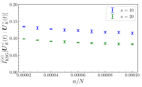
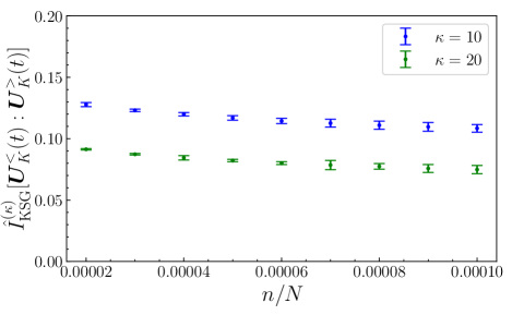
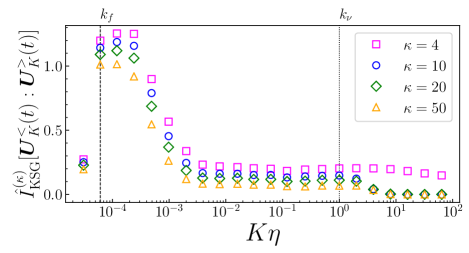
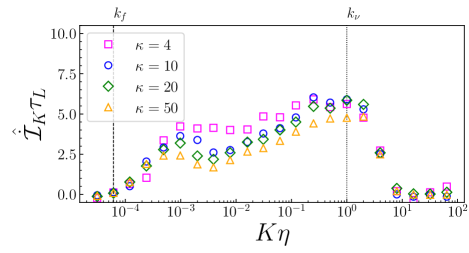
Figure 4: Bias of the KSG estimator $\hat{I}^{(\kappa)}_{\mathrm{KSG}}[{\bm{U}}^{<}_{K}(t):{\bm{U}}^{>}_{K}(t)]$ as a function of $1/N_{\mathrm{samp}}=n/N$ with $n=2,3,\cdots,10$ and $N=10^{5}$. $K=k_{10}$ (top) and $K=k_{15}$ (bottom).

Figure 5: Scale dependences of the estimated mutual information $\hat{I}^{(\kappa)}_{\mathrm{KSG}}[{\bm{U}}^{<}_{K}(t):{\bm{U}}^{>}_{K}(t)]$ (top) and information flow $\hat{\dot{\mathcal{I}}}_{K}$ (bottom). Note that the information flow is plotted in units of the inverse of $\tau_{L}$.

References

• Kolmogorov [1941a] A. N. Kolmogorov, The local structure of turbulence in incompressible viscous fluid for very large Reynolds numbers, Dokl. Akad. Nauk SSSR 30, 9 (1941a).
• Kolmogorov [1941b] A. N. Kolmogorov, On degeneration of isotropic turbulence in an incompressible viscous liquid, Dokl. Akad. Nauk SSSR 31, 538 (1941b).
• Kolmogorov [1941c] A. N. Kolmogorov, Dissipation of energy in locally isotropic turbulence, Dokl. Akad. Nauk SSSR 32, 16 (1941c).
• Frisch [1995] U. Frisch, Turbulence (Cambridge university press, 1995).
• Davidson [2015] P. A. Davidson, Turbulence: An Introduction for Scientists and Engineers, 2nd ed. (Oxford University Press, 2015).
• Anselmet et al. [1984] F. Anselmet, Y. l. Gagne, E. J. Hopfinger, and R. A. Antonia, High-order velocity structure functions in turbulent shear flows, J. Fluid Mech. 140, 63 (1984).
• Eyink and Sreenivasan [2006] G. L. Eyink and K. R. Sreenivasan, Onsager and the theory of hydrodynamic turbulence, Rev. Mod. Phys. 78, 87 (2006).
• [8] G. L. Eyink, Turbulence Theory, Course Notes, http://www.ams.jhu.edu/~eyink/Turbulence/notes/.
• Yasuda et al. [2014] T. Yasuda, S. Goto, and G. Kawahara, Quasi-cyclic evolution of turbulence driven by a steady force in a periodic cube, Fluid Dyn. Res. 46, 061413 (2014).
• Goto et al. [2017] S. Goto, Y. Saito, and G. Kawahara, Hierarchy of antiparallel vortex tubes in spatially periodic turbulence at high Reynolds numbers, Phys. Rev. Fluids 2, 064603 (2017).
• Araki et al. [2023] R. Araki, W. Bos, and S. Goto, Minimal model of quasi-cyclic behaviour in turbulence driven by taylor–green forcing, Fluid Dyn. Res. 55, 035507 (2023).
• Pecora and Carroll [1990] L. M. Pecora and T. L. Carroll, Synchronization in chaotic systems, Phys. Rev. Lett. 64, 821 (1990).
• Boccaletti et al. [2002] S. Boccaletti, J. Kurths, G. Osipov, D. Valladares, and C. Zhou, The synchronization of chaotic systems, Phys. Rep. 366, 1 (2002).
• Yoshida et al. [2005] K. Yoshida, J. Yamaguchi, and Y. Kaneda, Regeneration of small eddies by data assimilation in turbulence, Phys. Rev. Lett. 94, 014501 (2005).
• Lalescu et al. [2013] C. C. Lalescu, C. Meneveau, and G. L. Eyink, Synchronization of chaos in fully developed turbulence, Phys. Rev. Lett. 110, 084102 (2013).
• Vela-Martín [2021] A. Vela-Martín, The synchronisation of intense vorticity in isotropic turbulence, J. Fluid Mech. 913 (2021).
• Betchov [1964] R. Betchov, Measure of the intricacy of turbulence, Phys. Fluids 7, 1160 (1964).
• Ikeda and Matsumoto [1989] K. Ikeda and K. Matsumoto, Information theoretical characterization of turbulence, Phys. Rev. Lett. 62, 2265 (1989).
• Cerbus and Goldburg [2013] R. T. Cerbus and W. I. Goldburg, Information content of turbulence, Phys. Rev. E 88, 053012 (2013).
• Materassi et al. [2014] M. Materassi, G. Consolini, N. Smith, and R. De Marco, Information theory analysis of cascading process in a synthetic model of fluid turbulence, Entropy 16, 1272 (2014).
• Cerbus and Goldburg [2016] R. T. Cerbus and W. I. Goldburg, Information theory demonstration of the Richardson cascade, arXiv preprint arXiv:1602.02980  (2016).
• Goldburg and Cerbus [2016] W. I. Goldburg and R. T. Cerbus, Turbulence as information, arXiv preprint arXiv:1609.00471  (2016).
• Granero-Belinchon et al. [2016] C. Granero-Belinchon, S. G. Roux, and N. B. Garnier, Scaling of information in turbulence, Europhys. Lett. 115, 58003 (2016).
• Granero-Belinchón et al. [2018] C. Granero-Belinchón, S. G. Roux, and N. B. Garnier, Kullback-Leibler divergence measure of intermittency: Application to turbulence, Phys. Rev. E 97, 013107 (2018).
• Lozano-Durán et al. [2020] A. Lozano-Durán, H. J. Bae, and M. P. Encinar, Causality of energy-containing eddies in wall turbulence, J. Fluid Mech. 882 (2020).
• Shavit and Falkovich [2020] M. Shavit and G. Falkovich, Singular measures and information capacity of turbulent cascades, Phys. Rev. Lett. 125, 104501 (2020).
• Vladimirova et al. [2021] N. Vladimirova, M. Shavit, and G. Falkovich, Fibonacci turbulence, Phys. Rev. X 11, 021063 (2021).
• Lozano-Durán and Arranz [2022] A. Lozano-Durán and G. Arranz, Information-theoretic formulation of dynamical systems: Causality, modeling, and control, Phys. Rev. Research 4, 023195 (2022).
• Parrondo et al. [2015] J. M. Parrondo, J. M. Horowitz, and T. Sagawa, Thermodynamics of information, Nat. Phys. 11, 131 (2015).
• Ehrich and Sivak [2023] J. Ehrich and D. A. Sivak, Energy and information flows in autonomous systems, Front. Phys. 11, 155 (2023).
• Shiraishi [2023] N. Shiraishi, An Introduction to Stochastic Thermodynamics: From Basic to Advanced, Vol. 212 (Springer Nature, 2023).
• Barato et al. [2014] A. C. Barato, D. Hartich, and U. Seifert, Efficiency of cellular information processing, New J. Phys. 16, 103024 (2014).
• Sartori et al. [2014] P. Sartori, L. Granger, C. F. Lee, and J. M. Horowitz, Thermodynamic costs of information processing in sensory adaptation, PLoS Comput. Biol. 10, e1003974 (2014).
• Ito and Sagawa [2015] S. Ito and T. Sagawa, Maxwell’s demon in biochemical signal transduction with feedback loop, Nat. Commun. 6, 1 (2015).
• Hartich et al. [2016] D. Hartich, A. C. Barato, and U. Seifert, Sensory capacity: An information theoretical measure of the performance of a sensor, Phys. Rev. E 93, 022116 (2016).
• Amano et al. [2022] S. Amano, M. Esposito, E. Kreidt, D. A. Leigh, E. Penocchio, and B. M. W. Roberts, Insights from an information thermodynamics analysis of a synthetic molecular motor, Nat. Chem. 14, 530 (2022).
• Penocchio et al. [2022] E. Penocchio, F. Avanzini, and M. Esposito, Information thermodynamics for deterministic chemical reaction networks, J. Chem. Phys. 157, 034110 (2022).
• Landau and Lifshitz [1959] L. D. Landau and E. M. Lifshitz, Fluid Mechanics, Vol. 6 (Addision-Wesley, Reading, MA, 1959).
• De Zarate and Sengers [2006] J. M. O. De Zarate and J. V. Sengers, Hydrodynamic fluctuations in fluids and fluid mixtures (Elsevier, 2006).
• Ruelle [1979] D. Ruelle, Microscopic fluctuations and turbulence, Phys. Lett. A 72, 81 (1979).
• Komatsu et al. [2014] T. S. Komatsu, S. Matsumoto, T. Shimada, and N. Ito, A glimpse of fluid turbulence from the molecular scale, Int. J. Mod. Phys. C 25, 1450034 (2014).
• Bandak et al. [2021] D. Bandak, G. L. Eyink, A. Mailybaev, and N. Goldenfeld, Thermal noise competes with turbulent fluctuations below millimeter scales, arXiv preprint arXiv:2107.03184  (2021).
• Bandak et al. [2022] D. Bandak, N. Goldenfeld, A. A. Mailybaev, and G. Eyink, Dissipation-range fluid turbulence and thermal noise, Phys. Rev. E 105, 065113 (2022).
• Eyink and Jafari [2022] G. Eyink and A. Jafari, High schmidt-number turbulent advection and giant concentration fluctuations, Phys. Rev. Research 4, 023246 (2022).
• McMullen et al. [2022] R. M. McMullen, M. C. Krygier, J. R. Torczynski, and M. A. Gallis, Navier-Stokes Equations Do Not Describe the Smallest Scales of Turbulence in Gases, Phys. Rev. Lett. 128, 114501 (2022).
• Bell et al. [2022] J. B. Bell, A. Nonaka, A. L. Garcia, and G. Eyink, Thermal fluctuations in the dissipation range of homogeneous isotropic turbulence, J. Fluid Mech. 939 (2022).
• Maes [2021] C. Maes, Local detailed balance, SciPost Phys. Lect. Notes 32, 1 (2021).
• Tanogami [2022a] T. Tanogami, Violation of the second fluctuation-dissipation relation and entropy production in nonequilibrium medium, J. Stat. Phys. 187, 1 (2022a).
• Peliti and Pigolotti [2021] L. Peliti and S. Pigolotti, Stochastic Thermodynamics: An Introduction (Princeton University Press, 2021).
• Gardiner [2009] C. W. Gardiner, Handbook of Stochastic Methods, 4th ed. (Springer, Berlin, 2009).
• Cover and Thomas [2006] T. M. Cover and J. A. Thomas, Elements of Information Theory, 2nd ed. (Wiley-Interscience, Hoboken, NJ, 2006).
• Hartich et al. [2014] D. Hartich, A. C. Barato, and U. Seifert, Stochastic thermodynamics of bipartite systems: transfer entropy inequalities and a Maxwell’s demon interpretation, J. Stat. Mech. 2014, P02016 (2014).
• Matsumoto and Sagawa [2018] T. Matsumoto and T. Sagawa, Role of sufficient statistics in stochastic thermodynamics and its implication to sensory adaptation, Phys. Rev. E 97, 042103 (2018).
• Horowitz and Esposito [2014] J. M. Horowitz and M. Esposito, Thermodynamics with continuous information flow, Phys. Rev. X 4, 031015 (2014).
• Sekimoto [2010] K. Sekimoto, Stochastic Energetics (Springer, New York, 2010).
• Shiraishi and Sagawa [2015] N. Shiraishi and T. Sagawa, Fluctuation theorem for partially masked nonequilibrium dynamics, Phys. Rev. E 91, 012130 (2015).
• L’vov et al. [1998] V. S. L’vov, E. Podivilov, A. Pomyalov, I. Procaccia, and D. Vandembroucq, Improved shell model of turbulence, Phys. Rev. E 58, 1811 (1998).
• Biferale [2003] L. Biferale, Shell models of energy cascade in turbulence, Annu. Rev. Fluid Mech. 35, 441 (2003).
• Bohr et al. [1998] T. Bohr, M. H. Jensen, G. Paladin, and A. Vulpiani, Dynamical systems approach to turbulence (Cambridge university press, 1998).
• Kraskov et al. [2004] A. Kraskov, H. Stögbauer, and P. Grassberger, Estimating mutual information, Phys. Rev. E 69, 066138 (2004).
• Khan et al. [2007] S. Khan, S. Bandyopadhyay, A. R. Ganguly, S. Saigal, D. J. Erickson III, V. Protopopescu, and G. Ostrouchov, Relative performance of mutual information estimation methods for quantifying the dependence among short and noisy data, Phys. Rev. E 76, 026209 (2007).
• Holmes and Nemenman [2019] C. M. Holmes and I. Nemenman, Estimation of mutual information for real-valued data with error bars and controlled bias, Phys. Rev. E 100, 022404 (2019).
• Carbone and Bragg [2020] M. Carbone and A. D. Bragg, Is vortex stretching the main cause of the turbulent energy cascade?, J. Fluid Mech. 883, R2 (2020).
• Wilson [1975] K. G. Wilson, The renormalization group: Critical phenomena and the Kondo problem, Rev. Mod. Phys. 47, 773 (1975).
• Tanogami [2021] T. Tanogami, Theoretical analysis of quantum turbulence using the Onsager ideal turbulence theory, Phys. Rev. E 103, 023106 (2021).
• Tanogami [2022b] T. Tanogami, Reply to “Comment on ‘Theoretical analysis of quantum turbulence using the Onsager ideal turbulence theory’ ”, Phys. Rev. E 105, 027102 (2022b).
• Krstulovic et al. [2022] G. Krstulovic, V. L’vov, and S. Nazarenko, Comment on “Theoretical analysis of quantum turbulence using the Onsager ideal turbulence theory”, Phys. Rev. E 105, 027101 (2022).
• Skrbek et al. [2021] L. Skrbek, D. Schmoranzer, Š. Midlik, and K. R. Sreenivasan, Phenomenology of quantum turbulence in superfluid helium, Proc. Natl. Acad. Sci. U. S. A. 118 (2021).
• Tanogami and Sasa [2021] T. Tanogami and S.-i. Sasa, Van der Waals cascade in supercritical turbulence near a critical point, Phys. Rev. Research 3, L032027 (2021).
• Nazarenko [2011] S. Nazarenko, Wave Turbulence, Vol. 825 (Springer Science & Business Media, 2011).
• Zakharov et al. [1992] V. E. Zakharov, V. S. L’vov, and G. Falkovich, Kolmogorov spectra of turbulence I: Wave turbulence (Springer, Berlin, 1992).
• Tanogami and Sasa [2022] T. Tanogami and S.-i. Sasa, XY model for cascade transfer, Phys. Rev. Research 4, L022015 (2022).
• Tsubota et al. [2013] M. Tsubota, Y. Aoki, and K. Fujimoto, Spin-glass-like behavior in the spin turbulence of spinor Bose-Einstein condensates, Phys. Rev. A 88, 061601(R) (2013).
• Rodriguez-Nieva [2021] J. F. Rodriguez-Nieva, Turbulent relaxation after a quench in the Heisenberg model, Phys. Rev. B 104, L060302 (2021).
• Harada and Sasa [2006] T. Harada and S.-i. Sasa, Energy dissipation and violation of the fluctuation-response relation in nonequilibrium Langevin systems, Phys. Rev. E 73, 026131 (2006).
• Risken [1996] H. Risken, The Fokker-Planck Equation (Springer, 1996).
• Lord and Rougemont [2004] G. J. Lord and J. Rougemont, A numerical scheme for stochastic PDEs with Gevrey regularity, IMA J. Numer. Anal. 24, 587 (2004).