An updated metal-dependent theoretical scenario for Classical Cepheids

Abstract

To properly quantify possible residual systematic errors affecting the Classical Cepheid distance scale, a detailed theoretical scenario is recommended. By extending the set of nonlinear convective pulsation models published for $Z=0.02$ (De Somma et al., 2020b) to $Z=0.004$, $Z=0.008$ and $Z=0.03$, we provide a detailed homogeneous nonlinear model grid taking into account simultaneous variations of the mass-luminosity relation, the efficiency of super-adiabatic convection and the chemical composition. The dependence of the inferred Period-Radius, Period-Mass-Radius, and Period-Mass-Luminosity-Temperature relations on the input parameters is discussed for both the Fundamental and First Overtone modes. The trend of the instability strip getting redder as the metallicity increases is confirmed for the additional ML assumptions and mixing length values. From the obtained multi-filter light curves, we derive mean magnitudes and colors and in turn Period-Luminosity-Color and Period-Wesenheit relations for each assumed chemical composition, mass-luminosity relation and efficiency of super-adiabatic convection. Application to a well-studied sample of Cepheids in the Large Magellanic Cloud allows us to constrain the dependence of the inferred distance modulus on the assumed mass-luminosity relation, and the inclusion of the metallicity term in the derivation of Period-Wesenheit relations allows us, for each assumed mass-luminosity relation, to predict the metallicity dependence of the Cepheid distance scale. The obtained metal-dependent Period-Wesenheit relations are compared with recent results in the literature and applied to a sample of Gaia Early Data Release 3 Galactic Cepheids with known metal abundances to derive individual parallaxes. The comparison of these predictions with Gaia results is finally discussed.

1 Introduction

The application of Classical Cepheid (CC) Period-Luminosity (PL) and Period-Luminosity-Color (PLC) relations to the calibration of the cosmic distance scale represents one of the most important examples of a connection between stellar and extragalactic astrophysics. This stellar route to the extragalactic distance ladder has drawn a renewed interest in the last few years thanks to the results of the Gaia mission providing the most accurate distance determinations obtained so far for more than 1$\%$ of the Milky Way stellar content (see e.g. Gaia Collaboration et al., 2021) and the resulting Hubble constant values significantly deviating from early Universe measurements and determinations (see e.g. Riess et al., 2021a, b; Verde et al., 2019, and references therein), despite their reduced uncertainties.
On this basis, a detailed investigation of the systematic errors affecting the various rungs of the cosmic distance ladder, in particular the CC distance scale, is needed. Among the possible sources of uncertainty, the dependence of the coefficients of PL and PLC relations on chemical composition has been tested by several authors in previous works from both the observational and the theoretical point of view (see e.g. Anderson et al., 2016; Bono et al., 2010; Breuval et al., 2021; Fausnaugh et al., 2015; Freedman & Madore, 2011; Groenewegen, 2013; Kennicutt et al., 1998; Kodric et al., 2013; Macri et al., 2006; Pejcha & Kochanek, 2012; Riess et al., 2016, 2021c; Ripepi et al., 2019, 2020, 2021, 2022; Romaniello et al., 2008, 2022; Shappee & Stanek, 2011; Wielgórski et al., 2017, and references therein).
As no consensus has yet been reached, despite the contribution provided by the unprecedented accuracy of Gaia astrometric distances, our team is involved in a project devoted to the investigation of the effect of metallicity on the CC distance scale. From the observational point of view, we have started a long term program called “Cepheid–Metallicity in the Leavitt Law” (C-MetaLL) to directly measure the metallicity dependence of CC relations using only Galactic pulsators with accurate metallicities from high-resolution spectroscopy, in combination with optical and Near Infrared (NIR) photometry, and Gaia parallaxes (Ripepi et al., 2021). From the theoretical point of view, we are updating the metal-dependent pulsational scenario predicted by Bono et al. (1999); Marconi et al. (2005, 2010) by selecting the same chemical compositions of the corresponding evolutionary models presented by Hidalgo et al. (2018) and available at URL:http://basti-iac.oa-abruzzo.inaf.it and varying simultaneously, for the first time, the chemical composition, the Mass-Luminosity (ML) relation and the efficiency of super-adiabatic convection. This approach aims to provide a self-consistent framework to quantify a variety of possible systematic errors that have not been taken into account so far, in the use of CCs as primary distance indicators as well as young stellar population tracers.

The organization of the paper is as follows. In Section 2, we present the new model sets. The results, including the Instability Strip (IS) boundaries, the period, shape and amplitude of light and radial velocity curves and the Period-Radius (PR) and the Period-Mass-Radius (PMR) relations, are presented in Section 3. The transformation of the bolometric light curves into the photometric filters, the derivation of mean magnitudes and colors, and in turn, of multi-band PLC, Period-Wesenheit (PW) and metal-dependent Period-Wesenheit (PWZ) relations, are presented in Sections 4 and 5, respectively. The application of the derived PWZ relation in the Gaia bands to a sample of Gaia Early Data Release 3 (EDR3) CCs to derive theoretical parallaxes and in turn investigate the Gaia zero-point offset is presented in Section 6. Finally, the conclusions and the discussion of some future developments close the paper.

2 The extended set of pulsation models

By adopting the same approach and the same physical and numerical assumptions as in De Somma et al. (2020b) but varying the chemical composition, we built an extended and detailed grid of nonlinear convective pulsation models. We investigated the full amplitude behavior of the computed models in both the Fundamental (F) and the First Overtone (FO) modes. The new adopted chemical compositions are: $Z=0.004$ $Y=0.25$, $Z=0.008$ $Y=0.25$, $Z=0.03$ $Y=0.28$.

For each chemical composition, a wide mass range is adopted (from 3 to 11 $M_{\odot}$ with a step of 1$M_{\odot}$ and for each mass, three luminosity levels were considered in order to predict the effect of the ML relation on CC properties. In particular, a canonical luminosity level, i.e. models computed by neglecting core convective overshooting, rotation, and mass loss, labeled ‘case A‘, and two noncanonical luminosity levels, obtained by increasing the canonical luminosity level by $\Delta\log(L$/$L_{\odot})$=$~{}0.2\;dex$ and $\Delta\log(L$/$L_{\odot})$=$~{}0.4\;dex$, labeled ‘case B‘ and ‘case C‘, respectively, were adopted. For each combination of chemical composition, mass and luminosity, a wide range of effective temperatures (roughly from $3600$ to $7200K$ with a step of $100K$) and three values of the mixing length parameter describing convective efficiency, namely $\alpha_{ml}=1.5,1.7,1.9$ were taken into account. All the adopted parameters are reported in the first seven columns of Tables LABEL:f_param_model and LABEL:fo_param_model for F and FO-mode models, respectively.
These tables are available in their entirety as supplementary material. The behavior of the predicted pulsation relation connecting the period to M, L and $T_{e}$ and of the IS boundaries when varying the chemical composition was investigated in De Somma et al. (2021a), as well as the new theoretical metal-dependent Period-Age and Period-Age-Color relations and their application to observational data (see De Somma et al., 2021a, for details).
The combination of these new model sets with the already published framework for $Z=0.02$ $Y=0.28$ (see De Somma et al., 2020b, a, 2021b; Marconi et al., 2020) provides a theoretical scenario that simultaneously takes into account several possible sources of systematic effects in the prediction of CC pulsation properties and distance scale.

3 The new theoretical results

As a result of the nonlinear hydrodynamic computations, we obtained the full amplitude behavior of the investigated models in the first three radial modes. We found 696 F-mode, 110 FO-mode and 3 Second Overtone (SO) mode stable Cepheid pulsation models for $Z=0.004$, 639 F-mode, 126 FO-mode and 6 SO-mode stable Cepheid pulsation models for $Z=0.008$, and 127 F-mode and 4 stable FO-mode Cepheid pulsation models for $Z=0.03$. Pulsation in the second overtone mode was found only for a few low mass and metal-poor models so that we decided to focus only on the first two radial modes. The stable limit cycle pulsation period and mean radius (as resulting from an averaging operation of the radius curve), for each model, are reported in the last two columns of Tables LABEL:f_param_model and LABEL:fo_param_model.

Table 1: The intrinsic stellar parameters of Z=0.004 Y= 0.25, Z=0.008 Y= 0.25, and Z=0.03 Y= 0.28 computed F-mode models. This table is available in its entirety in machine readable form.

Z	Y	$M/M_{\odot}\,$	log ($L/L_{\odot})\,$	$T_{eff}$[K]	$\alpha_{ml}$	ML	P[d]	$\log(\overline{R}$/$R_{\odot})$
0.004	0.25	3.0	2.49	5900	1.5	A	1.46027	1.230
0.004	0.25	3.0	2.49	6000	1.5	A	1.38159	1.217
0.004	0.25	3.0	2.49	6000	1.7	A	1.38248	1.215
…
0.008	0.25	3.0	2.39	6000	1.5	A	1.15407	1.166
0.008	0.25	3.0	2.59	5700	1.5	B	2.00247	1.307
0.008	0.25	3.0	2.59	5800	1.5	B	1.88759	1.295
…
0.03	0.28	4.0	2.68	5400	1.5	A	2.42133	1.398
0.03	0.28	4.0	2.68	5500	1.5	A	2.28760	1.383
0.03	0.28	4.0	2.68	5600	1.5	A	2.14887	1.367
…

Table 2: The intrinsic stellar parameters of Z=0.004 Y= 0.25, Z=0.008 Y= 0.25, and Z=0.03 Y= 0.28 computed FO-mode models. This table is available in its entirety in machine readable form.

Z	Y	$M/M_{\odot}\,$	log ($L/L_{\odot})\,$	$T_{eff}$[K]	$\alpha_{ml}$	ML	P[d]	$\log(\overline{R}$/$R_{\odot})$
0.004	0.25	3.0	2.49	6100	1.5	A	0.96086	1.202
0.004	0.25	3.0	2.49	6200	1.5	A	0.91345	1.190
0.004	0.25	3.0	2.49	6300	1.5	A	0.86753	1.176
…
0.008	0.25	3.0	2.39	6100	1.5	A	0.79791	1.151
0.008	0.25	3.0	2.39	6200	1.5	A	0.75783	1.138
0.008	0.25	3.0	2.39	6300	1.5	A	0.72289	1.126
…
0.03	0.28	4.0	2.68	6000	1.5	A	1.21353	1.309
0.03	0.28	4.0	2.68	6100	1.5	A	1.15266	1.296
0.03	0.28	4.0	2.68	6200	1.5	A	1.09496	1.282

3.1 The Period-Radius and Period-Mass-Radius relations

An important aspect of Cepheid research concerns the use of CCs to infer stellar radii. According to the so-called pulsation relation, the period of a variable at a fixed chemical composition depends on its mean density i.e. on its stellar mass and radius (PMR relation). As such, that independent estimates of both period and mean radius provide an independent evaluation of Cepheid pulsation masses. By neglecting the mass dependence a Period-Radius relation is obtained. In this work we computed radius curves to derive time-averaged mean radii that were then correlated with the pulsation periods. As a result, we could obtain updated PR relations for both F and FO models, varying the chemical composition, the assumed ML relation and the efficiency of super-adiabatic convection. The coefficients of the inferred relations are reported in Table LABEL:pr_f_fo_all. In Fig. 1, the value of the intercept of our F and FO-mode PR relations (with the associated error) is reported on the x-axis and the value of the slope (with the associated error) is reported on the y axis, for Z = 0.004 (black dots), Z=0.008 (light blue dots), Z=0.02 (green dots taken from De Somma et al. (2020b)) and Z=0.03 (orange dot). This comparison shows that the effect of a variation in the chemical composition is almost negligible, thus suggesting the possibility of deriving a global relation through linear regression of all the periods and mean radii reported in Table 4.

We also found (see Fig. 2) that a variation in the assumed efficiency of super-adiabatic convection does not significantly affect the slope and the zero point of predicted PR relations. However, a change of the assumed ML relation from case A to case C (see Fig. 3) makes the PR relation flatter, thus predicting a smaller radius at a fixed period. The two grey dots in both Fig. 2 and Fig. 3 represent the slope and intercept of the PR relation at Z=0.02 for canonical F mode pulsators with $\alpha_{ml}=1.9$ and the slope and intercept at Z=0.03 for canonical FO mode pulsators with $\alpha_{ml}=1.5$. These cases are characterized by a very low number of models and the predicted coefficients are less reliable than the others.

The comparison of the PR relations predicted in this paper with independent empirical and semi-empirical relations available in the literature is shown in Figs 4, 5 and 6. In fig. 4 we compared the slope and intercept of our PR relations for $\alpha_{ml}=1.5$, different chemical compositions and ML assumptions, with the slope and intercept with their relative errors of both the empirical and theoretical PR relations taken from the literature (see labels in the plot). The dark grey and light grey areas are the $1\sigma$ error and $3\sigma$ error of the slope and intercept of our theoretical relations, respectively, to investigate the agreement between our relations and ones from the literature. It is shown a better agreement when the A or B cases for $Z=0.004$ and the B case for $Z=0.008$ are adopted. At the highest metal abundances, $Z=0.02$ and $Z=0.03$, it is more difficult to identify the nest ML case as the independent values in the literature are spread on wider ranges, even if the canonical A case seems to be globally less in agreement than B and C.

In Fig. 5 the F-mode PR relations for $Z=0.004$ (upper panels), $Z=0.008$ (middle panels) and $Z=0.02$ (bottom panels) derived by Bono et al. (1998) are subtracted from the ones derived in this paper for the A and B ML relation cases. The agreement is good, as easily expectable considering the adoption of the same hydrodynamical code. We performed this check only to account for the inclusion of a much finer model grid and a slightly different ML relation in the current paper.

In Fig. 6 the PR relations for $Z=0.006$ (light blue symbols) and $Z=0.002$ (orange symbols) provided by Anderson et al. (2016), are subtracted from the ones obtained in this work for $Z=0.004$ and $\alpha_{ml}=1.5$, as a function of the pulsational period, for various assumptions on the ML relation (see labels). We noticed that a better agreement is obtained with predictions for $Z=0.006$ than for $Z=0.002$. Moreover, as the Anderson et al. (2016) results are based on brighter models (noncanonical ML relation) which include both overshooting and rotation, we found a general better agreement with the Anderson et al. (2016) relations when considering our noncanonical (cases B and C ML relations) PR relations for both F and FO-modes.

If the width in temperature of the IS is neglected, the pulsation relation connecting the period of a variable, at fixed chemical composition, to the stellar mass, luminosity and effective temperature, can be converted into a period-mass-radius (PMR) relation. This means that independent estimates of both periods and mean radii provide an independent evaluation of Cepheid masses. Theoretical Period-Mass-Radius (PMR) relations are reported in Table LABEL:pmr_f_fo_all. Inspection of this Table suggests that the PMR relation depends on the assumed ML relation and, marginally, on the adopted metal content. In particular, for a short period variable (e.g. $\log P=0.3$) with $Z=0.004$, the predicted mean radius decreases by 1.4% from case A to B and by about 5% from case A to C. For a long period variable (e.g. $\log P=1.8$) at the same metallicity, the variation in the predicted mean radius decreases by up to 7% moving from case A to B and by up to 9% moving from case A to C. On the other hand, for canonical radii, an increase in the metal content from $Z=0.004$ to $Z=0.008$ and finally to $Z=0.03$ leads to a variation that ranges from 0.5% to almost 4%. Similar results on the metallicity dependence were obtained for noncanonical models. Similar to what is shown for the PR relation, we also derived cumulative PMR relations including all the chemical compositions but assumimg various $\alpha_{ml}$ values and ML relations. The coefficients are reported in Table 6.

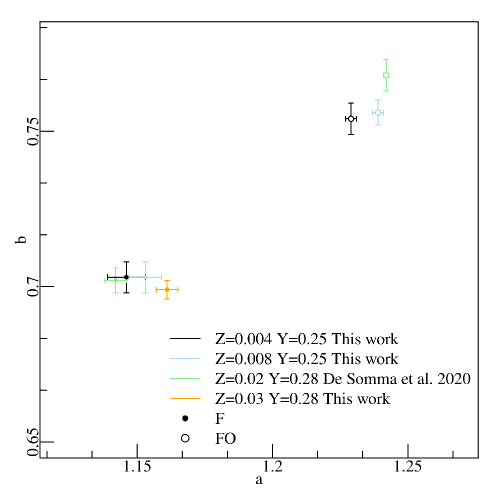
Figure 1: The intercept (a) and the slope (b) of the fitted canonical F and FO mode PR relations, at a fixed mixing length parameter $\alpha_{ml}=1.5$ for Z = 0.004 Y = 0.25 (black dots), Z = 0.008 Y = 0.25 (light blue dots), Z = 0.02 Y = 0.28 (green dots) and Z = 0.03 Y = 0.28 (orange dot). The coefficients for FO-mode pulsators are not shown for Z=0.03 because the models were too few to allow an accurate regression.

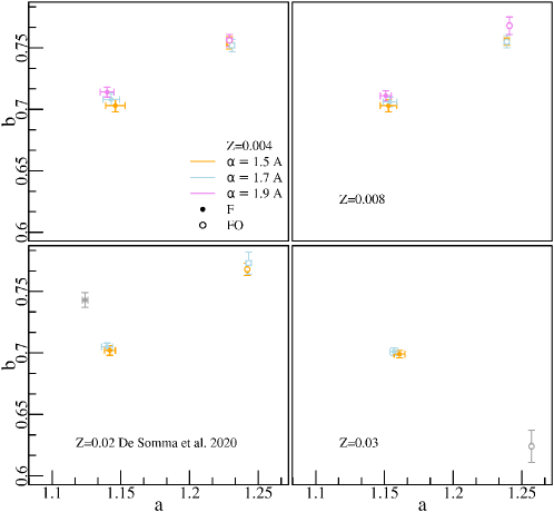
Figure 2: The intercept (a) and the slope (b) of the fitted canonical F and FO mode PR relations for Z = 0.004 Y = 0.25, Z = 0.008 Y = 0.25, Z = 0.02 Y = 0.28 (taken from De Somma et al. (2020b)) and Z = 0.03 Y = 0.28 as a function of the mixing length parameter (see text and labels for more details.

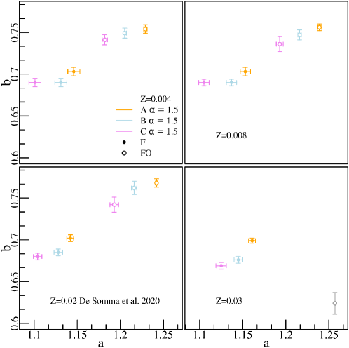
Figure 3: The intercept (a) and the slope (b) of the fitted F and FO mode PR relations for Z = 0.004 Y = 0.25, Z = 0.008 Y = 0.25, Z = 0.02 Y = 0.28 (taken from De Somma et al. (2020b)) and Z = 0.03 Y = 0.28, at a fixed mixing length parameter $\alpha_{ml}=1.5$, as a function of the various assumptions about the ML relation (see text and labels for more details.

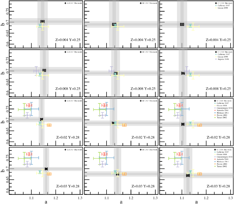
Figure 4: The intercept (a) and the slope (b) of the fitted theoretical PR relations for the F-mode pulsators and $\alpha_{ml}=1.5$ are compared to independent results available in the literature. The different panels show the results for different metallicity values, increasing from top (Z=0.004) to bottom (Z=0.03) and different cases for the assumed ML relation: A (left panels), B (middle panels) and C (right panels). In each panel, a (x-axis) and b (y-axis) with their uncertainties for all the considered assumptions are plotted. The theoretical results of this work are indicated with black symbols, while the literature results are plotted using different colors (see labels). The dark and light grey areas indicate the $1\sigma$ error and $3\sigma$ intervals, respectively, of both a and b values of our PR relations.

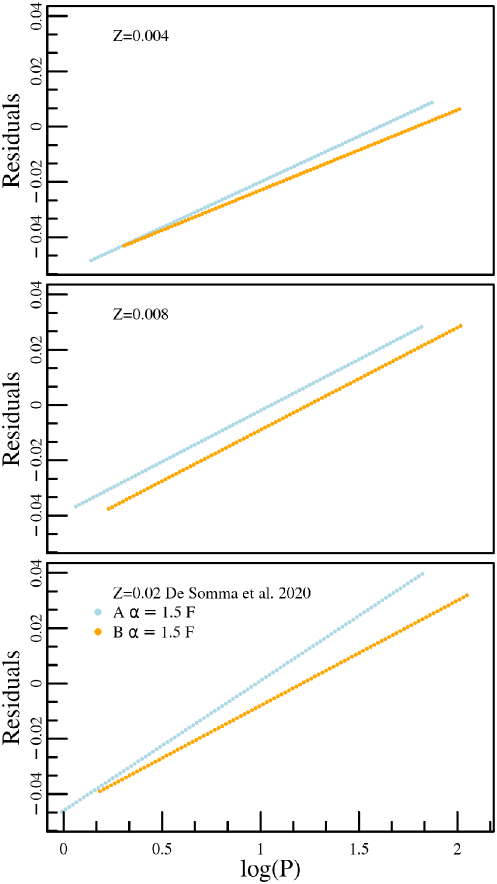
Figure 5: This figure shows the residuals, obtained by subtracting the PR relations for F pulsators provided by Bono et al. (1998) from the ones derived in this work, chosen as fiducial lines, as a function of the pulsational period. In the top, central and bottom panels, the results for Z = 0.004, Z=0.008, and Z = 0.02 are shown, respectively. In each panel, different ML assumptions are represented with different colors: light blue dots for the canonical case A, and orange dots for the non-canonical case B

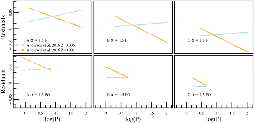
Figure 6: As in Fig 5, but subtracting the PR relations for Z=0.006 and Z=0.002 provided by Anderson et al. (2016), from the one obtained in this work for Z=0.004 and $\alpha_{ml}=1.5$, as a function of the pulsational period. The top and bottom panels show the results for the F and FO-mode pulsators, respectively. The left panels contain the results for the canonical case A while the central and right panels contain the results for the noncanonical cases B and C, respectively. In each panel, the residuals for Z=0.006 and Z = 0.002 are plotted using light blue and orange dots, respectively.

Table 3: The coefficients of the relation $\log$ ($R$/$R_{\odot}\,$)=a+b $\log P$ for both F and FO Cepheids derived by adopting Z=0.004 Y= 0.25, Z=0.008 Y= 0.25 and Z=0.03 Y= 0.28, as a function of the assumed $\alpha_{ml}$ parameter and ML relation.

$\alpha_{ml}$	ML	a	b	$\sigma_{a}$	$\sigma_{b}$	$R^{2}$
			Z=0.004	Y= 0.25
F
1.5	A	1.146	0.703	0.007	0.005	0.9958
1.5	B	1.131	0.690	0.007	0.005	0.9954
1.5	C	1.101	0.690	0.007	0.005	0.9955
1.7	A	1.143	0.708	0.006	0.005	0.9973
1.7	B	1.129	0.692	0.006	0.004	0.9970
1.7	C	1.104	0.687	0.006	0.004	0.9970
1.9	A	1.140	0.714	0.005	0.004	0.9984
1.9	B	1.128	0.694	0.005	0.004	0.9978
1.9	C	1.103	0.687	0.006	0.004	0.9978
FO
1.5	A	1.229	0.754	0.002	0.005	0.999
1.5	B	1.206	0.725	0.012	0.025	0.9800
1.5	C	1.182	0.741	0.003	0.006	0.9997
1.7	A	1.231	0.752	0.002	0.005	0.9993
1.7	B	1.209	0.713	0.014	0.032	0.9749
1.7	C	1.178	0.746	0.007	0.017	0.9989
1.9	A	1.229	0.756	0.002	0.005	0.9995
1.9	B	1.203	0.752	0.003	0.008	0.9995
			Z=0.008	Y= 0.25
F
1.5	A	1.153	0.703	0.006	0.005	0.9966
1.5	B	1.137	0.690	0.006	0.004	0.9961
1.5	C	1.105	0.690	0.006	0.004	0.9972
1.7	A	1.154	0.706	0.005	0.004	0.9979
1.7	B	1.137	0.689	0.006	0.004	0.9973
1.7	C	1.111	0.686	0.005	0.004	0.9978
1.9	A	1.151	0.711	0.004	0.004	0.9990
1.9	B	1.133	0.695	0.005	0.004	0.9986
1.9	C	1.115	0.683	0.005	0.003	0.9987
FO
1.5	A	1.239	0.756	0.002	0.004	0.9990
1.5	B	1.216	0.747	0.002	0.006	0.9988
1.5	C	1.193	0.736	0.004	0.009	0.9987
1.7	A	1.239	0.755	0.002	0.005	0.9992
1.7	B	1.215	0.747	0.002	0.006	0.9993
1.7	C	1.194	0.732	0.003	0.008	0.9993
1.9	A	1.241	0.768	0.001	0.007	0.9993
1.9	B	1.214	0.748	0.002	0.014	0.9984
1.9	C	1.220	0.573	0.001	0.003	1.0000
			Z=0.03	Y= 0.28
F
1.5	A	1.161	0.699	0.004	0.003	0.9988
1.5	B	1.145	0.676	0.005	0.004	0.9979
1.5	C	1.125	0.669	0.006	0.004	0.9975
1.7	A	1.157	0.701	0.003	0.003	0.9997
1.7	B	1.140	0.679	0.005	0.004	0.9991
1.7	C	1.122	0.670	0.005	0.003	0.9990
FO
1.5	A	1.257	0.624	0.001	0.013	0.9992

Table 4: The coefficients of the relation $\log$ ($R$/$R_{\odot}\,$)=a+b $\log P$ for both F and FO Cepheids derived by using all the models as a function of the assumed $\alpha_{ml}$ parameter and ML relation.

$\alpha_{ml}$	ML	a	b	$\sigma_{a}$	$\sigma_{b}$	$R^{2}$
F
1.5	A	1.148	0.703	0.003	0.002	0.9972
1.5	B	1.134	0.686	0.003	0.002	0.9964
1.5	C	1.103	0.687	0.004	0.003	0.9965
1.7	A	1.145	0.708	0.003	0.003	0.9978
1.7	B	1.132	0.689	0.003	0.002	0.9972
1.7	C	1.104	0.687	0.003	0.002	0.9976
1.9	A	1.142	0.715	0.003	0.003	0.9986
1.9	B	1.127	0.696	0.003	0.003	0.9982
1.9	C	1.104	0.688	0.003	0.002	0.9983
FO
1.5	A	1.238	0.740	0.003	0.008	0.9921
1.5	B	1.215	0.726	0.004	0.011	0.9903
1.5	C	1.193	0.729	0.003	0.007	0.9981
1.7	A	1.237	0.754	0.001	0.004	0.9989
1.7	B	1.214	0.721	0.005	0.014	0.9887
1.7	C	1.190	0.733	0.004	0.011	0.9976
1.9	A	1.235	0.754	0.002	0.006	0.9985
1.9	B	1.210	0.742	0.002	0.009	0.9982
1.9	C	1.212	0.621	0.002	0.012	0.9992

Table 5: The coefficients of the relation $\log$ $R$/$R_{\odot}\,$=a+b $\log$ P + c $\log$ M for both F and FO Cepheids derived by adopting Z=0.004 Y= 0.25, Z=0.008 Y= 0.25, and Z=0.03 Y= 0.28 as a function of the assumed $\alpha_{ml}$ parameter and ML relations.

$\alpha_{ml}$	ML	a	b	c	$\sigma_{a}$	$\sigma_{b}$	$\sigma_{c}$	$R^{2}$
				Z=0.004	Y= 0.25
F
1.5	A	0.893	0.520	0.541	0.009	0.006	0.018	0.9997
1.5	B	0.918	0.511	0.536	0.009	0.008	0.022	0.9994
1.5	C	0.948	0.515	0.503	0.009	0.010	0.027	0.9992
1.7	A	0.893	0.521	0.538	0.009	0.007	0.019	0.9998
1.7	B	0.909	0.506	0.550	0.009	0.008	0.022	0.9996
1.7	C	0.943	0.515	0.505	0.009	0.009	0.027	0.9995
1.9	A	0.884	0.517	0.551	0.011	0.009	0.024	0.9999
1.9	B	0.893	0.494	0.585	0.011	0.010	0.028	0.9997
1.9	C	0.930	0.506	0.533	0.010	0.010	0.030	0.9996
FO
1.5	A	0.720	0.365	0.988	0.061	0.044	0.117	0.9961
1.5	B	0.815	0.418	0.873	0.080	0.065	0.178	0.9920
1.5	C	1.072	0.636	0.288	0.022	0.021	0.056	1.0000
1.7	A	1.013	0.594	0.418	0.011	0.008	0.021	1.0000
1.7	B	0.709	0.335	1.105	0.097	0.076	0.214	0.9922
1.7	C	0.973	0.550	0.539	0.031	0.030	0.082	1.0000
1.9	A	1.000	0.586	0.441	0.029	0.022	0.056	0.9999
1.9	B	1.021	0.595	0.409	0.007	0.006	0.016	1.0000
				Z=0.008	Y= 0.25
F
1.5	A	0.907	0.542	0.490	0.008	0.005	0.016	0.9997
1.5	B	0.913	0.525	0.513	0.010	0.007	0.021	0.9994
1.5	C	0.956	0.543	0.437	0.010	0.009	0.027	0.9993
1.7	A	0.899	0.537	0.505	0.010	0.006	0.019	0.9999
1.7	B	0.881	0.503	0.581	0.010	0.007	0.023	0.9997
1.7	C	0.948	0.534	0.460	0.010	0.009	0.028	0.9995
1.9	A	0.898	0.538	0.501	0.014	0.010	0.028	0.9999
1.9	B	0.865	0.492	0.612	0.016	0.012	0.037	0.9998
1.9	C	0.917	0.509	0.539	0.015	0.014	0.042	0.9997
FO
1.5	A	1.012	0.595	0.416	0.009	0.006	0.016	1.0000
1.5	B	1.037	0.612	0.370	0.010	0.007	0.020	0.9999
1.5	C	1.045	0.617	0.351	0.009	0.007	0.021	1.0000
1.7	A	0.996	0.586	0.441	0.016	0.011	0.030	0.9999
1.7	B	1.025	0.600	0.397	0.009	0.007	0.018	1.0000
1.7	C	1.033	0.603	0.382	0.012	0.010	0.029	1.0000
1.9	A	1.020	0.611	0.397	0.019	0.013	0.034	1.0000
1.9	B	1.017	0.595	0.410	0.018	0.015	0.038	0.9999
				Z=0.03	Y= 0.28
F
1.5	A	0.886	0.545	0.500	0.019	0.011	0.035	0.9997
1.5	B	0.901	0.522	0.522	0.016	0.010	0.034	0.9995
1.5	C	0.960	0.434	0.537	0.012	0.030	0.009	0.9994
1.7	A	0.864	0.537	0.531	0.038	0.072	0.023	0.9999
1.7	B	0.853	0.617	0.494	0.028	0.061	0.018	0.9998
1.7	C	0.962	0.419	0.542	0.020	0.053	0.016	0.9996

Table 6: The coefficients of the relation $\log$ $R$/$R_{\odot}\,$=a+b $\log$ P + c $\log$ M for both F and FO Cepheids derived by using all the models as a function of the assumed $\alpha_{ml}$ parameter and ML relation.

$\alpha_{ml}$	ML	a	b	c	$\sigma_{a}$	$\sigma_{b}$	$\sigma_{c}$	$R^{2}$
F
1.5	A	0.916	0.554	0.460	0.008	0.005	0.015	0.9994
1.5	B	0.915	0.527	0.506	0.007	0.005	0.015	0.9991
1.5	C	0.954	0.539	0.446	0.006	0.006	0.018	0.9990
1.7	A	0.916	0.552	0.465	0.011	0.007	0.022	0.9994
1.7	B	0.896	0.512	0.550	0.009	0.007	0.020	0.9994
1.7	C	0.949	0.538	0.451	0.007	0.007	0.021	0.9993
1.9	A	0.930	0.564	0.435	0.012	0.008	0.024	0.9997
1.9	B	0.909	0.524	0.518	0.011	0.009	0.027	0.9995
1.9	C	0.941	0.534	0.468	0.010	0.009	0.028	0.9995
FO
1.5	A	0.924	0.531	0.577	0.026	0.018	0.047	0.9974
1.5	B	0.957	0.549	0.539	0.030	0.022	0.063	0.9963
1.5	C	1.057	0.626	0.322	0.006	0.005	0.014	0.9999
1.7	A	1.048	0.623	0.348	0.009	0.007	0.017	0.9999
1.7	B	0.909	0.512	0.639	0.048	0.034	0.100	0.9953
1.7	C	1.041	0.611	0.361	0.007	0.006	0.017	0.9999
1.9	A	1.031	0.613	0.379	0.010	0.007	0.018	0.9999
1.9	B	1.055	0.626	0.331	0.010	0.007	0.020	0.9999

3.2 The Period-Luminosity-Mass-Temperature relations

The pulsation relation derived from the combination of the definition of the pulsation period as a function of the stellar mean density (period-density relation) and the Stefan-Boltzmann law, is a Period-Luminosity-Mass-effective Temperature (hereinafter PLMT) relation, crucially connecting the characteristic oscillation time to structural parameters resulting from stellar evolution. We combined all the parameters reported in Tables LABEL:f_param_model and LABEL:fo_param_model to derive new PMLT relations (see Table 7) for each assumed chemical composition and both pulsation modes. As a result, we found that fundamental periods show a small correlation with the assumed metal content at a fixed mass, luminosity and effective temperature, whereas no significant dependence is found for first overtone models. On this basis, we also derived metal-dependent PLMT relations (hereinafter called PLMTZ relations) for F-mode models only. The coefficients and the intrinsic dispersion of the PLMTZ relations derived by varying the efficiency of the super-adiabatic convection are reported in Table 8. We noticed that the effect of a variation in the mixing length parameter is negligible within the error, thus confirming previous results obtained for solar chemical composition models (see De Somma et al., 2020b).

Table 7: The coefficients of the PMLT relations $\log P$ = a +b$\log T_{eff}$ + c $\log$ ($M/M_{\odot}\,$) + d log ($L/L_{\odot})\,$for both F and FO pulsators as a function of the assumed $\alpha_{ml}$ parameter for Z=0.004 Y= 0.25, Z=0.008 Y= 0.25 and Z=0.03 Y= 0.28.

$\alpha_{ml}$	a	b	c	d	$\sigma_{a}$	$\sigma_{b}$	$\sigma_{c}$	$\sigma_{d}$	$R^{2}$
				Z=0.004	Y= 0.25
F
1.5	10.711	-3.315	-0.776	0.918	0.109	0.028	0.017	0.005	0.9990
1.7	10.699	-3.312	-0.788	0.921	0.104	0.026	0.014	0.005	0.9995
1.9	10.764	-3.327	-0.791	0.919	0.124	0.031	0.014	0.005	0.9996
FO
1.5	12.042	-3.636	-0.574	0.799	0.271	0.325	0.112	0.037	0.9867
1.7	11.590	-3.524	-0.677	0.828	0.385	0.352	0.102	0.036	0.9929
1.9	11.182	-3.410	-0.591	0.801	0.434	0.111	0.023	0.009	0.9999
				Z=0.008	Y= 0.25
F
1.5	10.482	-3.254	-0.773	0.920	0.103	0.026	0.017	0.005	0.9991
1.7	10.588	-3.283	-0.777	0.922	0.110	0.028	0.015	0.005	0.9995
1.9	11.077	-3.405	-0.770	0.911	0.184	0.046	0.017	0.007	0.9996
FO
1.5	10.880	-3.337	-0.622	0.816	0.122	0.031	0.009	0.003	0.9999
1.7	10.927	-3.348	-0.622	0.813	0.223	0.057	0.014	0.005	0.9998
1.9	10.774	-3.300	-0.618	0.802	0.302	0.077	0.014	0.006	0.9998
				Z=0.03	Y= 0.28
F
1.5	10.414	-3.227	-0.765	0.918	0.119	0.029	0.023	0.008	0.9998

Table 8: The coefficients of the PMLTZ relations $\log P$ = a +b$\log T_{eff}$ + c $\log$ ($M/M_{\odot}\,$) + d log ($L/L_{\odot})\,$+ e [Fe/H] for both F and FO pulsators as a function of the assumed $\alpha_{ml}$ parameter obtained by using all the computed models for Z = 0.004 Y= 0.25, Z = 0.008 Y = 0.25, Z= 0.02 Y = 0.25 and Z = 0.03 Y = 0.28.

$\alpha_{ml}$	a	b	c	d	e	$\sigma_{a}$	$\sigma_{b}$	$\sigma_{c}$	$\sigma_{d}$	$\sigma_{e}$	$R^{2}$
F
1.5	10.513	-3.255	-0.772	0.919	0.046	0.054	0.014	0.009	0.003	0.002	0.9993
1.7	10.663	-3.295	-0.780	0.919	0.043	0.071	0.018	0.009	0.003	0.002	0.9995
1.9	10.891	-3.351	-0.783	0.914	0.036	0.107	0.027	0.011	0.004	0.003	0.9996

3.3 The new predicted instability strip

As a result of the integration of the nonlinear system of hydrodynamic equations, the limit cycle stability of each selected pulsation model was obtained and the topology of the instability strips for the aforementioned chemical compositions was derived. The effective temperatures of the inferred F and FO boundaries are reported in Tables LABEL:boundaries_smc, LABEL:boundaries_lmc and LABEL:boundaries_m31, for $Z=0.004$, $Z=0.008$ and $Z=0.03$, respectively, in Section A of the Appendix. In each table, columns from 1 to 8 report the mass, the luminosity level, the adopted mixing length parameter, the ML label and the effective temperatures for the First Overtone Blue Edge (FOBE), the Fundamental Blue Edge (FBE), the First Overtone Red Edge (FORE) and the Fundamental Red Edge (FRE).

A linear regression of the inferred boundary effective temperature values, as a function of the luminosity level, for different assumptions of the $\alpha_{ml}$ parameter, provides the relations reported in Tables 9, 11, 13, for the F and FO-mode respectively and varying the metal abundance from $Z=0.004$ to $Z=0.03$. The quadratic fit of the F-mode boundaries provides the relations reported in Tables 10, 12 and 14.

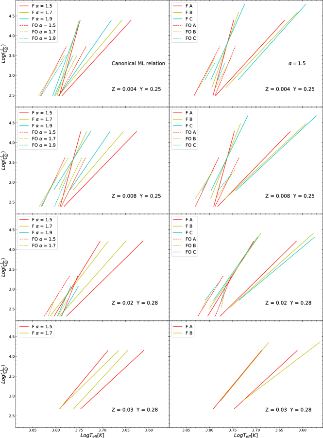
Figure 8: The F and FO instability strips for Z = 0.004 Y = 0.25, Z = 0.008 Y = 0.25, Z = 0.02 Y = 0.28 and Z = 0.03 Y = 0.28 pulsators at a fixed case A ML relation for the various assumptions about the superadiabatic convective efficiency (left panels) and at a fixed mixing length parameter $\alpha_{ml}=1.5$ for the assumed A, B, C ML relations (right panels).

Fig. 8 shows the linear relations for the predicted boundaries, at the labeled chemical compositions, varying both the super-adiabatic convective efficiency (left panels) and the ML assumption (right panels). These plots show that, in agreement with previous investigations (Bono et al., 1997, 1999) based on an earlier version of the same hydrodynamical code and an older version of the ML relation, a change in the chemical composition does significantly affect the topology of the instability strip. Indeed, as the metallicity increases from $Z=0.004$ to $Z=0.03$, at each fixed mixing length parameter and ML relation, the strip gets redder. The width of the instability strip decreases as the efficiency of super-adiabatic convection increases. This is particularly evident for the FO-mode that becomes less and less efficient till it disappears at super-solar metallicity ($Z=0.03$) for $\alpha_{ml}$=1.9. This occurrence is related to both the significant decrease of the Hydrogen abundance that reduces the efficiency of the more external FO-mode pulsation, and to the increased opacity related to the iron peak that enhances the convective efficiency and its damping effect on pulsation.

However, other authors (see e.g. Anderson et al., 2016) found a lower dependence of the instability strip morphology on the chemical composition based on linear nonadiabatic pulsation models. To test the accuracy of our predictions, in Fig. 7 we compared our theoretical boundaries for $Z=0.004$, $Z=0.008$ and $Z=0.02$ with available cepheid data with Gaia parallaxes. In particular, we adopted Gaia DR2 for SMC and LMC assuming a mean distance modulus of $\mu=18.977$ mag (Graczyk et al., 2020) and $\mu=18.48$ mag (Pietrzyński et al., 2019), respectively. On the other hand, the boundaries for $Z=0.02$ were compared with Cepheids with Gaia EDR3 individual distances based on the parallaxes with relative errors better than 10%. We noted that the agreement is generally good with a slightly better match for ML case A with $\alpha_{ml}=1.7$ for the Magellanic Clouds, at least for the assumed distance moduli. For the MW the situation is more confused but the best agreement seems to be obtained for the canonical ML relation with $\alpha_{ml}=1.5$ for the blue boundary and $\alpha_{ml}=1.7$ for the red boundary. The possibility that the assumed $\alpha_{ml}$ value varies across the instability strip was already discussed in previous papers (Di Criscienzo et al., 2004; Fiorentino et al., 2007).

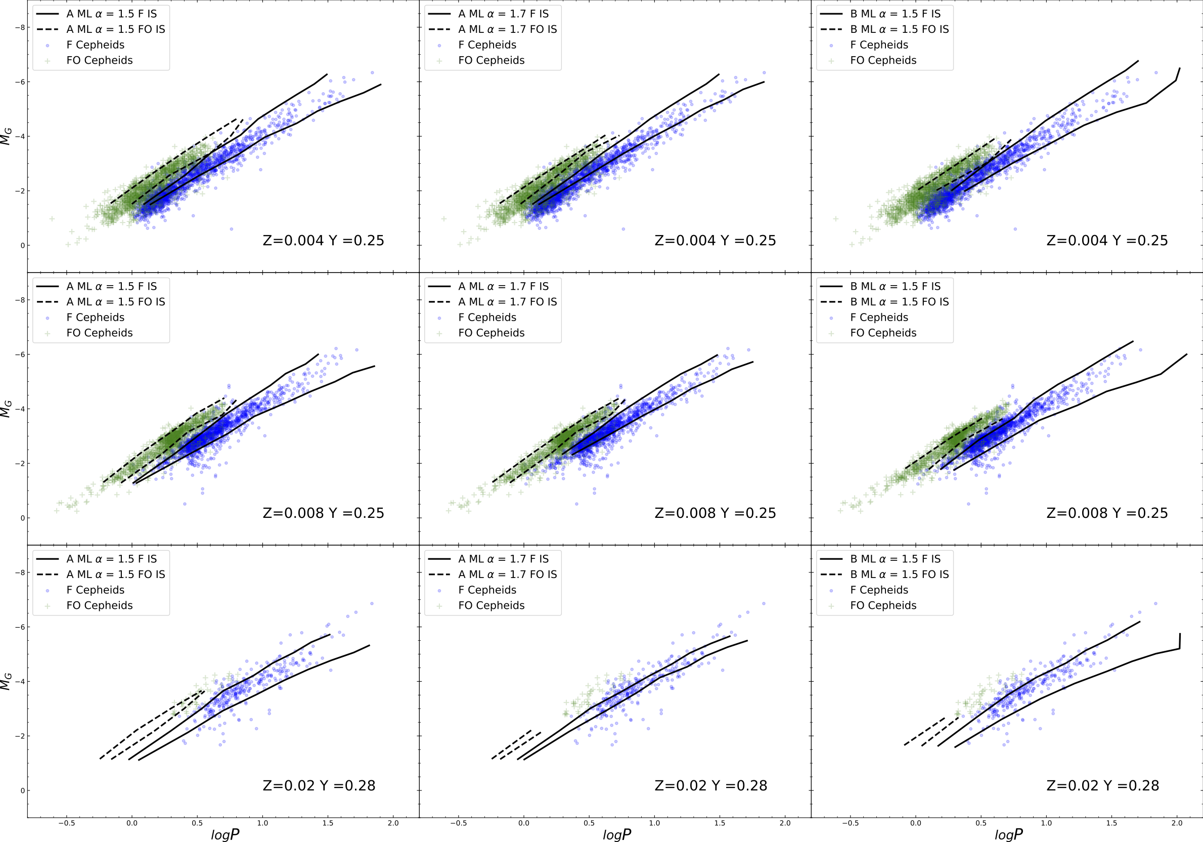
Figure 7: The location of F and FO-mode pulsators (green plus and blue points, respectively) for $Z=0.004$ (upper panels), $Z=0.008$ (middle panels) and $Z=0.02$ (bottom panels) in the $logP$-G plane. The solid and dashed black lines are the theoretical F and FO-mode instability strip boundaries, respectively, for the labeled ML and $\alpha_{ml}$ assumptions.

Table 9: The coefficients of the linear relation $\log T_{eff}$ = a +b log ($L/L_{\odot})\,$for the boundaries of the F and FO-mode IS for Z = 0.004 Y= 0.25 varying both the ML relation and the mixing length parameter.

$\alpha_{ml}$	ML	a	b	$\sigma_{a}$	$\sigma_{b}$	$R^{2}$
FOBE
1.5	A	3.941	-0.044	0.012	0.004	0.9796
1.5	B	3.945	-0.045	0.005	0.002	0.9988
1.7	A	3.971	-0.054	0.007	0.002	0.9963
1.7	B	3.970	-0.054	0.014	0.005	0.9932
1.9	A	3.961	-0.052	0.017	0.005	0.9791
1.9	B	3.966	-0.055	0.014	0.005	0.9931
FBE
1.5	A	3.825	-0.016	0.012	0.003	0.8717
1.5	B	3.849	-0.022	0.011	0.003	0.8879
1.5	C	3.889	-0.033	0.010	0.003	0.9589
1.7	A	3.842	-0.020	0.009	0.002	0.9075
1.7	B	3.876	-0.029	0.013	0.003	0.9188
1.7	C	3.911	-0.038	0.008	0.002	0.9803
1.9	A	3.873	-0.028	0.013	0.004	0.9009
1.9	B	3.895	-0.034	0.011	0.003	0.9565
1.9	C	3.924	-0.042	0.005	0.001	0.9939
FORE
1.5	A	3.844	-0.026	0.043	0.013	0.5588
1.5	B	3.888	-0.042	0.099	0.032	0.6320
1.7	A	3.870	-0.031	0.046	0.015	0.6807
1.7	B	3.894	-0.041	0.097	0.031	0.6321
1.9	A	3.882	-0.033	0.031	0.010	0.8443
1.9	B	3.867	-0.028	0.058	0.019	0.6879
FRE
1.5	A	3.958	-0.074	0.014	0.004	0.9814
1.5	B	3.937	-0.069	0.033	0.009	0.9031
1.5	C	3.762	-0.021	0.073	0.018	0.7445
1.7	A	3.941	-0.064	0.011	0.003	0.9840
1.7	B	3.949	-0.069	0.014	0.004	0.9819
1.7	C	3.825	-0.035	0.069	0.017	0.3785
1.9	A	3.920	-0.055	0.007	0.002	0.9918
1.9	B	3.950	-0.065	0.015	0.004	0.9758
1.9	C	3.860	-0.042	0.061	0.015	0.5236

Table 10: The coefficients of the quadratic relation $\log T_{eff}$ = a + b log ($L/L_{\odot})\,$+c (log ($L/L_{\odot})\,$)² for the boundaries of the F-mode IS for Z = 0.004 Y= 0.25 varying both the ML relation and the mixing length parameter.

$\alpha_{ml}$	ML	a	b	c	$\sigma_{a}$	$\sigma_{b}$	$\sigma_{c}$	$R^{2}$
FBE
1.5	A	3.708	0.054	-0.010	0.057	0.034	0.005	0.9003
1.5	B	3.681	0.072	-0.013	0.033	0.018	0.003	0.9791
1.5	C	3.740	0.047	-0.010	0.040	0.021	0.003	0.9878
1.7	A	3.734	0.045	-0.009	0.033	0.019	0.003	0.9676
1.7	B	3.674	0.084	-0.015	0.010	0.005	0.001	0.9989
1.7	C	3.847	-0.004	-0.004	0.053	0.028	0.004	0.9842
1.9	A	3.702	0.074	-0.015	0.039	0.023	0.003	0.9766
1.9	B	3.788	0.026	-0.008	0.055	0.031	0.004	0.9736
1.9	C	3.885	-0.021	-0.003	0.032	0.017	0.002	0.9951
FRE
1.5	A	3.776	0.035	-0.016	0.046	0.027	0.004	0.9950
1.5	B	4.157	-0.193	0.017	0.202	0.112	0.015	0.9195
1.5	C	4.917	-0.633	0.079	0.196	0.103	0.013	0.9199
1.7	A	3.789	0.026	-0.013	0.034	0.020	0.003	0.9964
1.7	B	3.880	-0.030	-0.005	0.087	0.048	0.007	0.9836
1.7	C	4.728	-0.515	0.062	0.316	0.166	0.021	0.7406
1.9	A	3.851	-0.014	-0.006	0.033	0.019	0.003	0.9953
1.9	B	3.738	0.053	-0.016	0.050	0.028	0.004	0.9940
1.9	C	4.520	-0.392	0.045	0.339	0.178	0.023	0.7108

Table 11: The coefficients of the linear relation $\log T_{eff}$ = a +b log ($L/L_{\odot})\,$for the boundaries of the F and FO-mode IS for Z = 0.008 Y= 0.25 varying both the ML relation and the mixing length parameter.

$\alpha_{ml}$	ML	a	b	$\sigma_{a}$	$\sigma_{b}$	$R^{2}$
FOBE
1.5	A	3.916	-0.037	0.021	0.007	0.9073
1.5	B	3.969	-0.054	0.013	0.004	0.9932
1.7	A	3.949	-0.048	0.020	0.006	0.9506
1.7	B	3.965	-0.054	0.014	0.005	0.9932
1.9	A	3.936	-0.044	0.024	0.009	0.9626
FBE
1.5	A	3.833	-0.020	0.012	0.003	0.8362
1.5	B	3.865	-0.029	0.017	0.005	0.8444
1.5	C	3.905	-0.040	0.013	0.003	0.9527
1.7	A	3.888	-0.035	0.020	0.005	0.8745
1.7	B	3.910	-0.041	0.024	0.006	0.8601
1.7	C	3.921	-0.044	0.012	0.003	0.9660
1.9	A	3.934	-0.048	0.025	0.007	0.8960
1.9	B	3.942	-0.051	0.020	0.005	0.9288
1.9	C	3.967	-0.058	0.012	0.003	0.9802
FORE
1.5	A	3.864	-0.034	0.029	0.009	0.8122
1.5	B	3.879	-0.039	0.078	0.026	0.6879
1.7	A	3.870	-0.034	0.029	0.009	0.8123
1.7	B	3.885	-0.038	0.076	0.025	0.6879
1.9	A	3.869	-0.029	0.040	0.014	0.8073
FRE
1.5	A	3.975	-0.081	0.014	0.004	0.9839
1.5	B	3.987	-0.087	0.022	0.006	0.9692
1.5	C	3.857	-0.050	0.058	0.015	0.6218
1.7	A	3.965	-0.072	0.011	0.003	0.9899
1.7	B	3.993	-0.084	0.026	0.007	0.9540
1.7	C	3.900	-0.058	0.050	0.013	0.7475
1.9	A	3.930	-0.058	0.009	0.002	0.9899
1.9	B	3.962	-0.069	0.015	0.004	0.9778
1.9	C	3.943	-0.066	0.038	0.010	0.8726

Table 12: The coefficients of the quadratic relation $\log T_{eff}$ = a + b log ($L/L_{\odot})\,$+c (log ($L/L_{\odot})\,$)² for the boundaries of the F-mode IS for Z = 0.008 Y= 0.25 varying both the ML relation and the mixing length parameter.

$\alpha_{ml}$	ML	a	b	c	$\sigma_{a}$	$\sigma_{b}$	$\sigma_{c}$	$R^{2}$
FBE
1.5	A	3.696	0.065	-0.013	0.044	0.026	0.004	0.9391
1.5	B	3.633	0.106	-0.019	0.061	0.035	0.005	0.9549
1.5	C	3.711	0.066	-0.014	0.046	0.025	0.003	0.9885
1.7	A	3.528	0.171	-0.029	0.066	0.038	0.005	0.9820
1.7	B	3.551	0.166	-0.029	0.044	0.025	0.004	0.9885
1.7	C	3.765	0.041	-0.011	0.056	0.031	0.004	0.9852
1.9	A	3.483	0.211	-0.036	0.069	0.040	0.006	0.9892
1.9	B	3.633	0.128	-0.025	0.030	0.017	0.002	0.9963
1.9	C	3.812	0.027	-0.011	0.056	0.031	0.004	0.9913
FRE
1.5	A	3.806	0.023	-0.015	0.049	0.030	0.004	0.9947
1.5	B	3.891	-0.031	-0.008	0.139	0.080	0.011	0.9715
1.5	C	4.646	-0.481	0.057	0.237	0.128	0.017	0.8691
1.7	A	3.820	0.011	-0.012	0.071	0.040	0.006	0.9946
1.7	B	3.607	0.139	-0.031	0.062	0.036	0.005	0.9939
1.7	C	4.482	-0.376	0.042	0.253	0.137	0.018	0.8674
1.9	A	3.936	-0.061	0.000	0.076	0.043	0.006	0.9899
1.9	B	3.768	0.043	-0.016	0.055	0.031	0.004	0.9929
1.9	C	4.159	-0.184	0.016	0.247	0.133	0.018	0.8873

Table 13: The coefficients of the linear relation $\log T_{eff}$ = a +b log ($L/L_{\odot})\,$for the boundaries of the F-mode IS for Z = 0.03 Y= 0.28 varying both the ML relation and the mixing length parameter.

$\alpha_{ml}$	ML	a	b	$\sigma_{a}$	$\sigma_{b}$	$R^{2}$
FBE
1.5	A	3.979	-0.070	0.007	0.002	0.9953
1.5	B	3.976	-0.070	0.009	0.002	0.9937
FRE
1.5	A	4.009	-0.096	0.015	0.004	0.9892
1.5	B	4.048	-0.111	0.013	0.004	0.9940

Table 14: The coefficients of the quadratic relation $\log T_{eff}$ = a + b log ($L/L_{\odot})\,$+c (log ($L/L_{\odot})\,$)² for the boundaries of the F-mode IS for Z = 0.03 Y= 0.28 varying both the ML relation and the mixing length parameter.

$\alpha_{ml}$	ML	a	b	c	$\sigma_{a}$	$\sigma_{b}$	$\sigma_{c}$	$R^{2}$
FBE
1.5	A	3.878	-0.010	-0.009	0.037	0.022	0.003	0.9981
1.5	B	3.957	-0.059	-0.001	0.076	0.042	0.006	0.9937
FRE
1.5	A	3.764	0.049	-0.021	0.052	0.031	0.004	0.9980
1.5	B	3.822	0.016	-0.017	0.059	0.033	0.005	0.9985

3.4 The new atlas of light and radial velocity curves

The computation of nonlinear pulsation models allowed us to predict variations of all relevant quantities, namely the luminosity, radius, radial velocity, surface temperature and gravity along a model pulsation cycle. The bolometric light curves for a sequence of canonical models listed in Tables LABEL:boundaries_smc to LABEL:boundaries_m31 shown in Section A of the Appendix are shown in the left panels of Figs 9 to 11, for each labeled mass, luminosity and mixing length parameter (labels at the top of each plot). The radial velocity curves of these models are represented in the right panels of the same plots. In these figures dotted lines refer to the few inferred SO-mode models, dashed lines correspond to FO-mode models, whereas solid lines represent F-mode models. The model period, in days, and the effective temperature, in kelvin, are also reported in the left and right panels, respectively. The entire atlas of light and radial velocity curves is available as supplementary material. We noticed that in agreement with previous investigations Bono et al. (see e.g. 2000a), the morphology and amplitude of both light and radial velocity curves are affected by a variation in the metal and helium abundance, as well as by the location inside the IS. We also notice a general decrease in the pulsation amplitudes as the metallicity increases, due to the increased contribution of opacity to convection. Quite interestingly, within the period range of 6 <P <16 days, CCs show the Hertzsprung progression phenomenon i.e. the evolution of the position in phase of the secondary maximum (bump) in both light and radial velocity curves, as a function of the pulsation period (Hertzsprung, 1926; Bono et al., 2000b). As expected, based on previous theoretical studies for 0.004 <Z <0.02 (see e.g. Bono et al., 2000b), an analysis of Figs 9, 10 and 11 suggests that an increase in the metal content causes a shift of the HP center (defined as the period at which the secondary bump reaches the same brightness as the primary one during its evolution from the decreasing to the rising branch of the curve) towards shorter periods. For example, passing from $Z=0.004$ to $Z=0.008$ and finally to $Z=0.02$ for a $M/M_{\odot}\,$= 7 model, the period corresponding to the HP center, in the case of canonical models, moves from about 11.4 to about 10.3 and finally decreases to about 7.5 days. A detailed investigation of the dependence on metallicity of the period corresponding to the HP center will be the subject of a future work (Marconi et al., in preparation).

Fig. Set9. Bolometric light and radial velocity curves for Z = 0.004 Y = 0.25

$M/M_{\odot}\,$=3.0    log ($L/L_{\odot})\,$=2.39    $\alpha_{ml}=1.5$

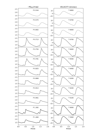
Figure 9: Bolometric light curves (left panel) and radial velocity curves (right panel) for a sequence of nonlinear F (solid line), FO (dashed lines) and if any SO (dotted lines) mode models (dashed lines) derived for Z = 0.004 Y = 0.25 at a fixed mass, luminosity, $\alpha_{ml}$ parameter (see labeled values on the top of the plot) adopting the canonical ML relation. The complete figure set (9 images) is available in the online journal.

Fig. Set9. Bolometric light and radial velocity curves for Z = 0.008 Y = 0.25

$M/M_{\odot}\,$=3.0    log ($L/L_{\odot})\,$=2.39    $\alpha_{ml}=1.5$

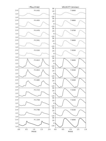
Figure 10: Bolometric light curves (left panel) and radial velocity curves (right panel) for a sequence of nonlinear F (solid line), FO (dashed lines) and if any SO (dotted lines) mode models (dashed lines) derived for Z = 0.008 Y = 0.25 at a fixed mass, luminosity, $\alpha_{ml}$ parameter (see labeled values on the top of the plot) adopting the canonical ML relation. The complete figure set (9 images) is available in the online journal.

Fig. Set8. Bolometric light and radial velocity curves for Z = 0.03 Y = 0.28

$M/M_{\odot}\,$=4.0    log ($L/L_{\odot})\,$=2.68    $\alpha_{ml}=1.5$

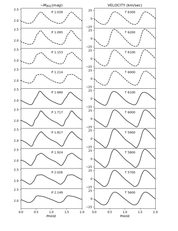
Figure 11: Bolometric light curves (left panel) and radial velocity curves (right panel) for a sequence of non linear F (solid line) and FO (dashed lines) models derived for Z = 0.03 Y = 0.28, at fixed mass, luminosity and $\alpha_{ml}$ parameter (see labeled values on the top of the plot) adopting the canonical ML relation. The complete figure set (8 images) is available in the online journal.

4 The predicted multifilters light curves

To facilitate observational comparisons, the bolometric light curves obtained from the nonlinear model computations have been transformed into various photometric filters, namely the three Gaia bands $G$, $G_{BP}$ and $G_{RP}$, the HST WFC3 filters F110W, F160W, F814W, F125W, F475W, F606W and F555W and the Johnson-Cousins (JC) bands U, B, V, R, J, H, K by adopting PHOENIX model atmospheres (Chen et al., 2019). The complete multi-filter atlas, obtained by varying the chemical composition, the ML relation and the efficiency of super-adiabatic convection, is available as supplementary material.

4.1 Mean magnitudes, colors and pulsation amplitudes

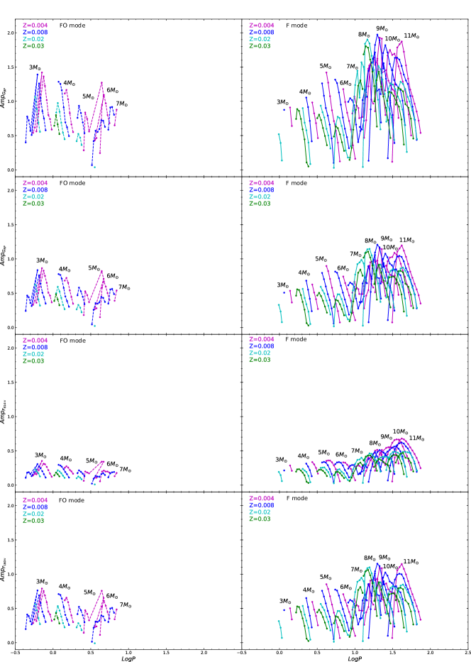
Figure 14: From top to bottom, the left panels show the FO-mode theoretical amplitudes for the $G_{BP}$ and $G_{RP}$ Gaia bands and the F814W and F160W HST-WFC3 bands for Z = 0.004 Y = 0.25 (dashed magenta line), Z = 0.008 Y = 0.25 (dashed blue line), Z = 0.02 Y = 0.28 (dashed cyan line) and Z = 0.03 Y = 0.28 (dashed green line) at fixed mixing length parameter $\alpha_{ml}=1.5$ and ML relation case A. The right panels show the same plots but for F-mode models (solid lines with the same color-code as in the left panels).

From the transformed light curves, we derived the intensity weighted mean magnitudes and the pulsation amplitudes reported in Tables 15 to 18 for the various filter combinations and the two pulsation modes. Mean colors are obtained as differences between couples of mean magnitudes and used to derive PLC and PW relations (see next section). In Fig. 14 shown in Section B of the appendix, the predicted multi-filter amplitudes are plotted as a function of the pulsation period for F (right panels) and FO (left panels), models for the labeled metal contents, assuming the case A (canonical) ML relation and $\alpha_{ml}$=1.5. We notice that, in agreement with previous theoretical results (see e.g. Bono et al., 2000a), the pulsation amplitudes tend to decrease as the metallicity increases. Moreover, F-mode amplitudes show a linear trend with the pulsation periods at the lowest luminosity levels. On the other hand, at higher luminosities, in a range where the FO-mode pulsation is no more efficient, the F-mode amplitudes show the same bell-shape displayed by FO models at lower luminosity levels. Figures from 15 to 21 shown in Section B of the appendix display the effect of a variation of $\alpha_{ml}$ (left panels) and the assumed ML relation (right panels) for all the chemical compositions and both F and FO-mode models, in the same filters as Fig.14 shown in Section B of the appendix. We notice that independently of the assumed abundances, the predicted pulsation amplitudes decrease as $\alpha_{ml}$ increases, down to the total quenching of pulsation for the more metallic FO sets at $\alpha=1.9$ and F amplitude values close to zero for $Z=0.03$ at $\alpha_{ml}=1.7$. On the other hand, the main effect of a variation of the ML relation is a shift of the covered period range, in both pulsation modes, to longer values, as the ML relation moves from case A to C. To test these theoretical predictions we used a sample of Magellanic Cepheids in the Gaia DR2 database (Gaia Collaboration et al., 2018) for which amplitudes in the Gaia $G_{BP}$ and $G_{RP}$ bands are available. In Figures 22 to 25 shown in Section B of the appendix, we compared the predicted period-amplitude diagram in the Gaia $G_{BP}$ and $G_{RP}$ filters at Z=0.008 and Z=0.004 to Gaia LMC and SMC results, respectively. In each figure, the upper and middle panels show the comparison between observed and theoretical amplitudes obtained for the canonical ML relation with $\alpha_{ml}=1.5$ and $1.7$, respectively, while the bottom panel shows the comparison for the B-case ML relation with $\alpha_{ml}=1.5$ . In general, we noticed that the period range of F and FO mode pulsators is well reproduced by canonical models both in the LMC and the SMC, apart from the lack of observed Cepheids at the longest predicted periods. Moreover, in the case of Z=0.008, we notice that the combination of a canonical ML relation with $\alpha_{ml}=1.5$ tends to predict higher amplitudes than observed, in particular at the shortest and longest periods, whereas the assumption of $\alpha_{ml}=1.7$ seems to better reproduce the data. The adoption of a brighter ML relation (case B) provides a satisfactory agreement for what concerns the amplitudes but seems to predict a period range shifted towards longer values with respect to the observations. Similar conclusions can be drawn in the case of Z=0.004.

Table 15: Mean magnitudes and theoretical amplitudes in the Gaia DR3 filters for the computed F-mode models with Z=0.004 Y= 0.25, Z=0.008 Y= 0.25, Z=0.02 Y= 0.28 and Z=0.03 Y= 0.28. This table is available in its entirety in machine readable form.

Z	Y	$M/M_{\odot}\,$	log ($L/L_{\odot})\,$	$T_{eff}$[K]	$\alpha_{ml}$	ML	G.m	G.amp	$G_{BP}.m$	$G_{BP}.amp$	$G_{RP}.m$	$G_{RP}.amp$
0.004	0.25	3.0	2.49	5900	1.5	A	-1.700	0.521	-1.457	0.640	-2.099	0.365
0.004	0.25	3.0	2.49	6000	1.5	A	-1.703	0.751	-1.472	0.910	-2.087	0.536
0.004	0.25	3.0	2.49	6000	1.7	A	-1.705	0.408	-1.475	0.500	-2.087	0.285
0.004	0.25	3.0	2.49	6100	1.7	A	-1.707	0.647	-1.488	0.783	-2.075	0.459
…
0.008	0.25	3.0	2.39	6000	1.5	A	-1.468	0.718	-1.228	0.876	-1.859	0.507
0.008	0.25	3.0	2.59	5700	1.5	B	-1.958	0.350	-1.678	0.436	-2.399	0.249
0.008	0.25	3.0	2.59	5800	1.5	B	-1.963	0.611	-1.696	0.745	-2.387	0.442
0.008	0.25	3.0	2.59	5900	1.5	B	-1.967	0.776	-1.714	0.936	-2.375	0.570
…
0.02	0.28	3.0	2.32	5900	1.5	A	-1.322	0.109	-1.054	0.137	-1.744	0.077
0.02	0.28	3.0	2.32	6000	1.5	A	-1.326	0.321	-1.071	0.392	-1.731	0.233
0.02	0.28	3.0	2.32	6100	1.5	A	-1.330	0.428	-1.090	0.520	-1.716	0.330
0.02	0.28	3.0	2.32	6100	1.7	A	-1.331	0.166	-1.092	0.204	-1.718	0.120
…
0.03	0.28	4.0	2.68	5400	1.5	A	-2.186	0.039	-1.822	0.050	-2.712	0.029
0.03	0.28	4.0	2.68	5500	1.5	A	-2.196	0.086	-1.849	0.109	-2.704	0.064
0.03	0.28	4.0	2.68	5600	1.5	A	-2.198	0.357	-1.870	0.445	-2.686	0.260
0.03	0.28	4.0	2.68	5700	1.5	A	-2.206	0.486	-1.896	0.591	-2.675	0.373
…

Table 16: Mean magnitudes and theoretical amplitudes in the Gaia DR3 filters for the computed FO-mode models with Z=0.004 Y= 0.25, Z=0.008 Y= 0.25, Z=0.02 Y= 0.28 and Z=0.03 Y= 0.28. This table is available in its entirety in machine readable form.

Z	Y	$M/M_{\odot}\,$	log ($L/L_{\odot})\,$	$T_{eff}$[K]	$\alpha_{ml}$	ML	G.m	G.amp	$G_{BP}.m$	$G_{BP}.amp$	$G_{RP}.m$	$G_{RP}.amp$
0.004	0.25	3.0	2.49	6100	1.5	A	-1.708	0.495	-1.490	0.588	-2.076	0.367
0.004	0.25	3.0	2.49	6200	1.5	A	-1.711	0.626	-1.504	0.740	-2.062	0.464
0.004	0.25	3.0	2.49	6300	1.5	A	-1.713	0.681	-1.519	0.800	-2.046	0.506
0.004	0.25	3.0	2.49	6400	1.5	A	-1.713	0.872	-1.533	1.018	-2.027	0.650
…
0.008	0.25	3.0	2.39	6100	1.5	A	-1.474	0.477	-1.248	0.578	-1.847	0.349
0.008	0.25	3.0	2.39	6200	1.5	A	-1.476	0.622	-1.263	0.752	-1.832	0.442
0.008	0.25	3.0	2.39	6300	1.5	A	-1.477	0.713	-1.277	0.856	-1.816	0.510
0.008	0.25	3.0	2.39	6400	1.5	A	-1.478	0.881	-1.292	1.047	-1.798	0.640
…
0.02	0.28	3.0	2.32	6200	1.5	A	-1.333	0.453	-1.107	0.555	-1.703	0.319
0.02	0.28	3.0	2.32	6300	1.5	A	-1.335	0.564	-1.123	0.689	-1.687	0.409
0.02	0.28	3.0	2.32	6400	1.5	A	-1.336	0.736	-1.138	0.884	-1.668	0.531
0.02	0.28	3.0	2.32	6500	1.5	A	-1.335	0.884	-1.152	1.063	-1.646	0.624
…
0.03	0.28	4.0	2.68	6000	1.5	A	-2.227	0.432	-1.964	0.522	-2.642	0.324
0.03	0.28	4.0	2.68	6100	1.5	A	-2.233	0.549	-1.985	0.663	-2.627	0.410
0.03	0.28	4.0	2.68	6200	1.5	A	-2.236	0.663	-2.005	0.799	-2.610	0.485
0.03	0.28	4.0	2.68	6300	1.5	A	-2.241	0.533	-2.022	0.643	-2.598	0.387

Table 17: Mean magnitudes and theoretical amplitudes in the HST-WFC3 filters for the computed F-mode models with Z=0.004 Y= 0.25, Z=0.008 Y= 0.25, Z=0.02 Y= 0.28 and Z=0.03 Y= 0.28. This table is available in its entirety in machine readable form.

Z	Y	$M/M_{\odot}\,$	log ($L/L_{\odot})\,$	$T_{eff}$[K]	$\alpha_{ml}$	ML	F110W.m	F110W.amp	F160W.m	F160W.amp	F814W.m	F814W.amp	F125W.m	F125W.amp	F475W.m	F475W.amp	F606W.m	F606W.amp	F555W.m	F555W.amp
0.004	0.25	3.0	2.49	5900	1.5	A	-2.435	0.245	-2.765	0.188	-2.152	0.342	-2.543	0.208	-1.315	0.713	-1.707	0.535	-1.520	0.616
0.004	0.25	3.0	2.49	6000	1.5	A	-2.409	0.372	-2.724	0.266	-2.137	0.505	-2.512	0.319	-1.338	1.009	-1.711	0.769	-1.532	0.880
0.004	0.25	3.0	2.49	6000	1.7	A	-2.404	0.170	-2.712	0.140	-2.137	0.268	-2.506	0.137	-1.342	0.557	-1.713	0.419	-1.535	0.483
0.004	0.25	3.0	2.49	6100	1.7	A	-2.380	0.293	-2.674	0.215	-2.123	0.432	-2.478	0.245	-1.362	0.868	-1.717	0.661	-1.547	0.758
…
0.008	0.25	3.0	2.39	6000	1.5	A	-2.174	0.319	-2.482	0.193	-1.908	0.478	-2.276	0.260	-1.090	0.976	-1.481	0.732	-1.298	0.842
0.008	0.25	3.0	2.59	5700	1.5	B	-2.764	0.149	-3.122	0.118	-2.456	0.235	-2.880	0.122	-1.515	0.491	-1.968	0.359	-1.758	0.415
0.008	0.25	3.0	2.59	5800	1.5	B	-2.737	0.276	-3.079	0.207	-2.441	0.419	-2.848	0.224	-1.543	0.829	-1.974	0.625	-1.774	0.714
0.008	0.25	3.0	2.59	5900	1.5	B	-2.709	0.373	-3.034	0.257	-2.426	0.541	-2.815	0.318	-1.570	1.036	-1.980	0.792	-1.789	0.900
…
0.02	0.28	3.0	2.32	5900	1.5	A	-2.064	0.049	-2.372	0.037	-1.795	0.073	-2.168	0.043	-0.896	0.155	-1.344	0.112	-1.141	0.130
0.02	0.28	3.0	2.32	6000	1.5	A	-2.036	0.163	-2.327	0.125	-1.779	0.221	-2.136	0.150	-0.922	0.439	-1.349	0.326	-1.155	0.374
0.02	0.28	3.0	2.32	6100	1.5	A	-2.005	0.249	-2.278	0.172	-1.762	0.318	-2.099	0.225	-0.950	0.579	-1.354	0.435	-1.170	0.498
0.02	0.28	3.0	2.32	6100	1.7	A	-2.004	0.087	-2.274	0.065	-1.764	0.115	-2.098	0.078	-0.952	0.229	-1.356	0.169	-1.171	0.195
…
0.03	0.28	4.0	2.68	5400	1.5	A	-3.128	0.018	-3.528	0.011	-2.774	0.028	-3.258	0.015	-1.598	0.058	-2.201	0.041	-1.934	0.048
0.03	0.28	4.0	2.68	5500	1.5	A	-3.102	0.041	-3.482	0.028	-2.765	0.061	-3.226	0.036	-1.638	0.125	-2.214	0.090	-1.958	0.105
0.03	0.28	4.0	2.68	5600	1.5	A	-3.064	0.173	-3.426	0.122	-2.744	0.248	-3.184	0.155	-1.672	0.508	-2.218	0.369	-1.974	0.428
0.03	0.28	4.0	2.68	5700	1.5	A	-3.034	0.260	-3.376	0.162	-2.730	0.358	-3.148	0.230	-1.711	0.669	-2.229	0.500	-1.997	0.569
…

Table 18: Mean magnitudes and theoretical amplitudes in the HST-WFC3 filters for the computed FO-mode models with Z=0.004 Y= 0.25, Z=0.008 Y= 0.25, Z=0.02 Y= 0.28 and Z=0.03 Y= 0.28. This table is available in its entirety in machine readable form.

Z	Y	$M/M_{\odot}\,$	log ($L/L_{\odot})\,$	$T_{eff}$[K]	$\alpha_{ml}$	ML	F110W.m	F110W.amp	F160W.m	F160W.amp	F814W.m	F814W.amp	F125W.m	F125W.amp	F475W.m	F475W.amp	F606W.m	F606W.amp	F555W.m	F555W.amp
0.004	0.25	3.0	2.49	6100	1.5	A	-2.378	0.251	-2.670	0.119	-2.124	0.348	-2.476	0.212	-1.363	0.646	-1.718	0.506	-1.548	0.572
0.004	0.25	3.0	2.49	6200	1.5	A	-2.350	0.323	-2.625	0.163	-2.108	0.440	-2.443	0.273	-1.385	0.811	-1.722	0.638	-1.560	0.720
0.004	0.25	3.0	2.49	6300	1.5	A	-2.321	0.373	-2.580	0.215	-2.090	0.481	-2.409	0.327	-1.408	0.876	-1.725	0.692	-1.572	0.780
0.004	0.25	3.0	2.49	6400	1.5	A	-2.288	0.480	-2.531	0.264	-2.068	0.619	-2.370	0.413	-1.431	1.111	-1.725	0.880	-1.583	0.990
…
0.008	0.25	3.0	2.39	6100	1.5	A	-2.142	0.237	-2.425	0.107	-1.894	0.331	-2.238	0.198	-1.117	0.641	-1.489	0.486	-1.314	0.557
0.008	0.25	3.0	2.39	6200	1.5	A	-2.113	0.306	-2.380	0.155	-1.877	0.416	-2.204	0.260	-1.140	0.833	-1.492	0.633	-1.326	0.725
0.008	0.25	3.0	2.39	6300	1.5	A	-2.083	0.339	-2.335	0.198	-1.858	0.481	-2.169	0.292	-1.163	0.948	-1.494	0.723	-1.338	0.827
0.008	0.25	3.0	2.39	6400	1.5	A	-2.051	0.449	-2.287	0.241	-1.838	0.607	-2.132	0.378	-1.187	1.151	-1.496	0.890	-1.350	1.011
…
0.02	0.28	3.0	2.32	6200	1.5	A	-1.976	0.208	-2.232	0.124	-1.747	0.300	-2.066	0.174	-0.975	0.620	-1.359	0.461	-1.183	0.531
0.02	0.28	3.0	2.32	6300	1.5	A	-1.945	0.281	-2.185	0.168	-1.727	0.388	-2.029	0.243	-1.001	0.769	-1.361	0.572	-1.196	0.660
0.02	0.28	3.0	2.32	6400	1.5	A	-1.912	0.367	-2.136	0.198	-1.706	0.502	-1.991	0.306	-1.026	0.978	-1.363	0.743	-1.208	0.849
0.02	0.28	3.0	2.32	6500	1.5	A	-1.876	0.433	-2.084	0.223	-1.682	0.590	-1.950	0.359	-1.049	1.176	-1.362	0.885	-1.218	1.017
…
0.03	0.28	4.0	2.68	6000	1.5	A	-2.946	0.227	-3.229	0.125	-2.689	0.310	-3.044	0.196	-1.810	0.582	-2.255	0.441	-2.054	0.502
0.03	0.28	4.0	2.68	6100	1.5	A	-2.915	0.290	-3.180	0.155	-2.672	0.391	-3.008	0.249	-1.841	0.738	-2.261	0.559	-2.072	0.636
0.03	0.28	4.0	2.68	6200	1.5	A	-2.882	0.343	-3.130	0.179	-2.653	0.461	-2.969	0.292	-1.872	0.889	-2.266	0.671	-2.088	0.768
0.03	0.28	4.0	2.68	6300	1.5	A	-2.853	0.273	-3.081	0.138	-2.638	0.367	-2.935	0.230	-1.896	0.715	-2.271	0.539	-2.101	0.618

5 The updated Period-Luminosity-Color and the Period-Wesenheit relations in the optical and near-infrared filters

The obtained intensity-weighted mean magnitudes and colors are used to derive updated theoretical PLC and PW relations for different filter combinations varying the pulsation mode, the chemical composition, the ML relation and the $\alpha_{ml}$ parameter. PL relations are being derived in an accompanying paper (Musella et al. in preparation) investigating their dependence on the Cepheid distribution inside the predicted instability strip boundaries, in a variety of photometric bands. Tables LABEL:plc_gaia and LABEL:plc_hst in Section C of the Appendix provide the PLC coefficients for F and FO-mode in the Gaia EDR3 filters ($<G>$=a+b$\log P$ +c($<G_{BP}>$ - $<G_{RP}>$) and HST-WFC filters ($<F_{160W}>$=a+b$\log P$ +c($<F_{555W}>$ - $<F_{814W}>$), respectively, while Tables LABEL:plc_johI and LABEL:plc_johK reported in the same section of the Appendix provide the PLC coefficients for two different Johnson-Cousins filter combinations ($<V>$ = a + b$\log P$ +c($<V>$ - $<I>$); $<V>$ = a + b$\log P$ +c($<V>$ - $<K>$)). The coefficients of the PW relations in the Gaia EDR3, HST-WFC3 and Johnson-Cousins filters are instead reported in Tables LABEL:pw_gaia to LABEL:pw_joh_K in Section D of the Appendix. In each of the aforementioned tables, apart from the chemical composition, we report the $\alpha_{ml}$ parameter, the selected ML case, the coefficients of the relations with their relative errors, the root-mean-square deviation ($\sigma$) and the R-squared ($R^{2}$) coefficients. To take into account the non-negligible metallicity effect on the predicted pulsation properties, we also derived the first theoretical PWZ relations for each different assumption on the $\alpha_{ml}$ parameter and the ML relation, for the four adopted filter combinations and the two pulsation modes. The coefficients are reported in Tables LABEL:pwz_gaia to LABEL:pwz_johK (See Table captions for more details). Inspection of these tables suggests that a small metallicity effect is predicted for the adopted filter combinations, thus confirming the advantage of using PW relations instead of simple PL relations to infer the extragalactic distance scale (see Fiorentino et al., 2007, for details). Indeed, for an uncertainty of $\sim 0.1$ dex on the metal abundance of the investigated pulsators, a distance modulus error depending on the filter, ML and $\alpha_{ml}$ combination, but generally smaller than $0.02$-$0.03$ mag, is expected.

5.1 The comparison with published PWZ relations

The inferred theoretical PWZ relations can be tested against current empirical determinations in the literature. Some of the most recent published PWZ relations are listed in Table 23. We notice that the metallicity coefficient of the PWZ relations predicted in this paper and reported in Tables LABEL:pwz_gaia and LABEL:pwz_johK is significantly smaller than in the corresponding empirical relations derived by Ripepi et al. (2021) and Ripepi et al. (2022) for F and fundamentalized FO-mode Galactic Cepheids, in the Gaia and the V and K filters, respectively. A better agreement is found between our PWZ relation in the JC V, I filters (see TableLABEL:pwz_johI) and the relation provided by Breuval et al. (2021) for a sample of MW, LMC and SMC CCs. The reason for the discrepancy between the predicted metallicity effect and the result by Ripepi et al. could be related to the different metallicity range of the selected observational and model samples and deserves further investigation.

Table 19: PWZ coefficients in the Gaia EDR3 filters ( W ($G$, $G_{BP}$-$G_{RP}$)=a + b ($\log P$ -1) +c [Fe/H]) for F and FO CCs derived by adopting A, B, C ML relations and $\alpha_{ml}$ = 1.5, 1.7 and 1.9.

$\alpha_{ml}$	ML	a	b	c	$\sigma_{a}$	$\sigma_{b}$	$\sigma_{c}$	$\sigma$	$R^{2}$
F
1.5	A	-6.018	-3.314	-0.189	0.009	0.016	0.021	0.118	0.993
1.7	A	-6.072	-3.379	-0.129	0.010	0.016	0.021	0.090	0.996
1.9	A	-6.170	-3.472	-0.245	0.023	0.018	0.040	0.072	0.998
1.5	B	-5.853	-3.234	-0.190	0.011	0.016	0.022	0.139	0.991
1.7	B	-5.871	-3.262	-0.260	0.012	0.015	0.023	0.118	0.995
1.9	B	-5.968	-3.370	-0.189	0.026	0.017	0.047	0.092	0.997
1.5	C	-5.694	-3.270	-0.105	0.012	0.017	0.023	0.141	0.991
1.7	C	-5.722	-3.274	-0.140	0.012	0.015	0.022	0.116	0.994
1.9	C	-5.800	-3.327	-0.167	0.023	0.016	0.043	0.094	0.997
FO
1.5	A	-6.676	-3.450	-0.221	0.051	0.048	0.059	0.145	0.985
1.7	A	-6.818	-3.627	-0.243	0.040	0.034	0.049	0.073	0.996
1.9	A	-6.933	-3.688	-0.349	0.045	0.030	0.052	0.034	0.999
1.5	B	-6.634	-3.566	-0.304	0.063	0.063	0.062	0.097	0.988
1.7	B	-6.616	-3.533	-0.303	0.095	0.083	0.095	0.103	0.987
1.9	B	-6.719	-3.627	-0.304	0.066	0.050	0.068	0.030	0.998
1.5	C	-6.473	-3.510	-0.235	0.043	0.051	0.038	0.038	0.996
1.7	C	-6.486	-3.506	-0.261	0.049	0.056	0.051	0.030	0.998

Table 19: continued.

Table 20: PWZ coefficients in the HST-WFC3 filters (W (F160W, F555W-F814W)=a + b ($\log P$ -1) +c [Fe/H]) for F and FO CCs derived by adopting A, B, C ML relations and $\alpha_{ml}$ = 1.5, 1.7 and 1.9.

$\alpha_{ml}$	ML	a	b	c	$\sigma_{a}$	$\sigma_{b}$	$\sigma_{c}$	$\sigma$	$R^{2}$
F
1.5	A	-6.023	-3.340	-0.161	0.008	0.015	0.019	0.109	0.994
1.7	A	-6.060	-3.393	-0.135	0.010	0.015	0.020	0.085	0.997
1.9	A	-6.155	-3.484	-0.195	0.022	0.017	0.038	0.067	0.998
1.5	B	-5.858	-3.254	-0.125	0.010	0.015	0.021	0.129	0.993
1.7	B	-5.865	-3.280	-0.121	0.011	0.014	0.021	0.110	0.995
1.9	B	-5.952	-3.376	-0.136	0.025	0.016	0.045	0.088	0.997
1.5	C	-5.702	-3.274	-0.145	0.011	0.016	0.021	0.127	0.993
1.7	C	-5.717	-3.281	-0.130	0.011	0.014	0.020	0.104	0.995
1.9	C	-5.782	-3.329	-0.110	0.022	0.015	0.040	0.088	0.997
FO
1.5	A	-6.684	-3.477	-0.105	0.048	0.045	0.056	0.137	0.987
1.7	A	-6.821	-3.651	-0.131	0.037	0.031	0.046	0.067	0.997
1.9	A	-6.930	-3.710	-0.240	0.038	0.025	0.045	0.029	0.999
1.5	B	-6.643	-3.595	-0.186	0.059	0.059	0.058	0.090	0.990
1.7	B	-6.627	-3.568	-0.192	0.091	0.080	0.091	0.099	0.989
1.9	B	-6.723	-3.653	-0.204	0.061	0.046	0.062	0.027	0.999
1.5	C	-6.499	-3.573	-0.125	0.034	0.041	0.030	0.030	0.998
1.7	C	-6.518	-3.576	-0.162	0.041	0.046	0.042	0.025	0.998

Table 20: continued.

Table 21: PWZ coefficients in the Johnson-Cousins filters (W(V,I)=a + b ($\log P$ -1) +c [Fe/H]) for F and FO CCs derived by adopting A, B, C ML relations and $\alpha_{ml}$ = 1.5, 1.7 and 1.9.

$\alpha_{ml}$	ML	a	b	c	$\sigma_{a}$	$\sigma_{b}$	$\sigma_{c}$	$\sigma$	$R^{2}$
F
1.5	A	-6.118	-3.341	-0.150	0.008	0.015	0.019	0.108	0.994
1.7	A	-6.162	-3.396	-0.175	0.010	0.015	0.020	0.085	0.997
1.9	A	-6.248	-3.483	-0.175	0.022	0.017	0.038	0.068	0.998
1.5	B	-5.957	-3.269	-0.101	0.010	0.014	0.020	0.125	0.993
1.7	B	-5.969	-3.289	-0.104	0.011	0.014	0.021	0.108	0.995
1.9	B	-6.045	-3.381	-0.119	0.025	0.016	0.045	0.089	0.997
1.5	C	-5.799	-3.298	-0.123	0.011	0.015	0.020	0.124	0.993
1.7	C	-5.821	-3.298	-0.111	0.011	0.014	0.020	0.104	0.996
1.9	C	-5.877	-3.338	-0.097	0.022	0.016	0.041	0.090	0.997
FO
1.5	A	-6.774	-3.490	-0.174	0.049	0.045	0.056	0.138	0.987
1.7	A	-6.916	-3.666	-0.200	0.037	0.031	0.045	0.066	0.997
1.9	A	-7.030	-3.731	-0.301	0.036	0.024	0.042	0.027	0.999
1.5	B	-6.733	-3.610	-0.252	0.060	0.059	0.058	0.091	0.990
1.7	B	-6.718	-3.581	-0.255	0.092	0.081	0.092	0.100	0.988
1.9	B	-6.817	-3.672	-0.256	0.049	0.038	0.051	0.022	0.999
1.5	C	-6.574	-3.564	-0.188	0.035	0.042	0.031	0.031	0.998
1.7	C	-6.591	-3.566	-0.216	0.040	0.046	0.042	0.025	0.998

Table 21: continued.

Table 22: PWZ coefficients in the Johnson-Cousins filters (W(V,K)=a + b ($\log P$ -1) +c [Fe/H]) for F and FO CCs derived by adopting A, B, C ML relations and $\alpha_{ml}$ = 1.5, 1.7 and 1.9.

$\alpha_{ml}$	ML	a	b	c	$\sigma_{a}$	$\sigma_{b}$	$\sigma_{c}$	$\sigma$	$R^{2}$
F
1.5	A	-6.016	-3.382	-0.145	0.008	0.014	0.018	0.101	0.995
1.7	A	-6.041	-3.419	-0.138	0.009	0.014	0.019	0.081	0.997
1.9	A	-6.126	-3.496	-0.177	0.021	0.017	0.037	0.067	0.998
1.5	B	-5.856	-3.300	-0.190	0.009	0.014	0.019	0.117	0.994
1.7	B	-5.858	-3.316	-0.195	0.010	0.013	0.020	0.101	0.996
1.9	B	-5.924	-3.388	-0.200	0.025	0.016	0.044	0.087	0.997
1.5	C	-5.702	-3.311	-0.107	0.010	0.014	0.019	0.113	0.994
1.7	C	-5.712	-3.312	-0.198	0.010	0.013	0.018	0.094	0.996
1.9	C	-5.755	-3.340	-0.106	0.021	0.015	0.039	0.086	0.997
FO
1.5	A	-6.656	-3.482	-0.089	0.048	0.045	0.056	0.136	0.987
1.7	A	-6.790	-3.655	-0.114	0.038	0.031	0.046	0.068	0.997
1.9	A	-6.899	-3.713	-0.227	0.040	0.026	0.047	0.030	0.999
1.5	B	-6.614	-3.599	-0.170	0.059	0.059	0.058	0.090	0.990
1.7	B	-6.598	-3.573	-0.177	0.091	0.080	0.091	0.099	0.989
1.9	B	-6.692	-3.656	-0.193	0.064	0.049	0.066	0.029	0.998
1.5	C	-6.473	-3.585	-0.108	0.034	0.041	0.030	0.030	0.998
1.7	C	-6.491	-3.586	-0.147	0.041	0.047	0.043	0.025	0.998

Table 22: continued.

Table 23: The PWZ relations (W=a + b ($\log P$ -1) +c [Fe/H]) recently derived by various authors for different CC samples. $\sigma$ is the predicted root-mean-square deviation coefficient.

authors	sample	bands	a	b	c	$\sigma_{a}$	$\sigma_{b}$	$\sigma_{c}$	$\sigma$
Breuval et al. (2021)	MW-LMC-SMC CC	JC V-I	-5.9893	-3.281	-0.251	0.008	0.022	0.057
Ripepi et al. (2021)	F-FO MW-CC	JC V-K	-6.022	-3.174	-0.459	0.022	0.049	0.107
Ripepi et al. (2022)	F-FO MW-CC	G-$G_{BP}$-$G_{RP}$	-5.988	-3.176	-0.520	0.018	0.044	0.090	0.014

5.2 The predicted distance of the Large Magellanic Cloud: effect of adopted ML relation

To quantify the impact of a variation of the ML relation on theoretical distance determinations, we applied the PW relations obtained for $Z=0.008$ to the OGLE catalog of LMC Cepheids (Soszyński et al., 2017). To evaluate the influence of a variation of the ML relation on the distance scale based on predicted relations and, in turn, on the final theoretically obtained $H_{0}$ value, we considered the derived PW relations in the Johnson-Cousins V and I filters for $Z=0.008$ with $\alpha_{ml}=1.5$ and ML cases A, B, and C. Application of these theoretical PW relations to the LMC Cepheids provided the distance moduli reported in Table 24. As expected, a variation of $\Delta\log(L$/$L_{\odot})$=$~{}0.2\;dex$ in the assumed ML relation (e.g. between cases A and B or between cases B and C) produces a variation in the inferred LMC distance modulus of $\sim$ 0.1 dex. This exercise shows that if a variation of the Cepheid ML relation occurred from galaxy to galaxy the assumption of a unique calibrating PW relation could produce systematic errors on the inferred distances.

Table 24: The distance moduli of LMC F-mode CCs obtained with the theoretical PW relations in the Johnson-Cousins V and I filters for $Z=0.008$ with $\alpha_{ml}=1.5$ and ML cases A, B, and C.

source	$\mu$	$\alpha_{ml}$	ML
F CC LMC	18.667	1.5	A
F CC LMC	18.555	1.5	B
F CC LMC	18.403	1.5	C

6 The predicted parallaxes of Galactic Cepheids

Following the same approach as De Somma et al. (2020b), we selected a sample of Galactic Cepheids with available periods, $G$, $G_{BP}$ and $G_{RP}$ magnitudes and Gaia EDR3 parallaxes. After being ensured that the parallax zero-point offset was corrected according to Lindegren et al. (2021) (see Ripepi et al., 2021, for details on this procedure), we derived the predicted distances and parallaxes of each Galactic Cepheid in the sample through the application of PW relations. In particular, we considered F and FO-mode Galactic Cepheids for which the G band magnitude is higher than 6. Moreover, as good astrometry is ensured by using sources for which the Renormalized Unit Weight Error (RUWE) coefficient is lower than 1.4 (Ripepi et al., 2021), we made this assumption in the target selection. The theoretical PWZ relations obtained in Section 5 in the Gaia filters, were applied to the selected sample in order to obtain reddening free individual distances and in turn theoretical parallaxes, through inversion of the predicted distances. The theoretical parallaxes were compared with the corresponding Gaia EDR3 values for the selected stars. The different panels of Fig. 12 show the difference between theoretical and Gaia parallaxes as a function of Gaia parallaxes (solid lines) compared with the value estimated for the Gaia zero-point offset published by Riess et al. (2021a) . The comparison is shown for each assumption about the mixing length parameter and the ML relation (see labels on the plot for details). From these plots, we can conclude that the combination of $\alpha_{ml}$ and ML that is most consistent with the value found by Riess et al. (2021a) corresponds to the canonical ML relation (case A models) with $\alpha_{ml}$ =1.7. In order to quantify the impact of the metallicity term on the inferred offsets, we repeated the analysis using the theoretical parallaxes based on the PW relations at a fixed solar metallicity (See Fig. 13). Again we found that the best match with the result by Riess et al. (2021a) is obtained for the canonical ML relation with $\alpha_{ml}=1.7$. Moreover, we notice that, for each assumed efficiency of super-adiabatic convection, the agreement with the offset by Riess et al. (2021a) tends to worsen as the ML relation gets brighter. This occurrence holds independently of the inclusion of a metallicity term in the PW relation.

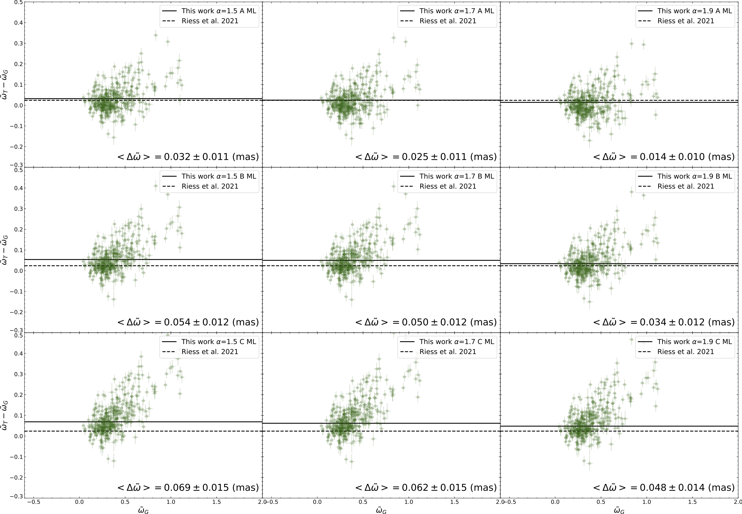
Figure 12: Parallax difference between the theoretical parallax obtained by adopting the PWZ relation and Gaia parallax ($\varpi_{T}$ - $\varpi_{G}$) as a function of Gaia EDR3 parallax $\varpi_{G}$, for F-mode Galactic Cepheids.

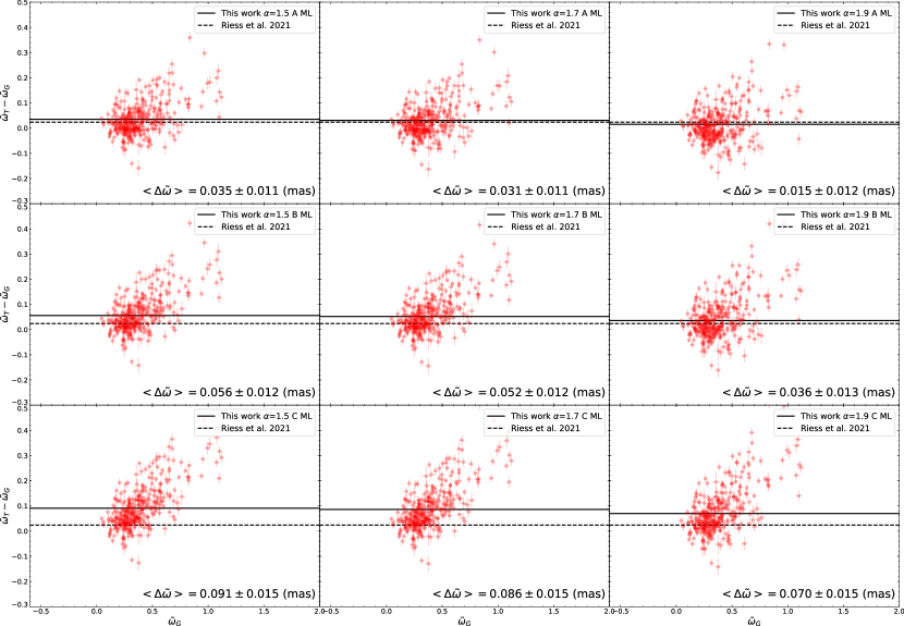
Figure 13: The same as Fig.12 but with the theoretical parallax obtained by applying the PW relation for $Z=0.02$.

7 Conclusions and Future Developments

Based on an extended and detailed grid of nonlinear convective pulsation models, built by systematically varying different physical and numerical ingredients, we have presented an updated metal-dependent theoretical scenario for Classical Cepheids. By extending the model set for solar chemical abundances, published in De Somma et al. (2020b), we have computed new nonlinear convective pulsation models for three additional chemical compositions, namely $Z=0.004$ $Y=0.25$, $Z=0.008$ $Y=0.25$ and $Z=0.02$ $Y=0.28$, three different assumptions about the ML relation and three adopted values of $\alpha_{ml}$. From the integration of the nonlinear system of dynamical and convective equations, we have derived the modal stability for both F and FO-mode pulsators. As a result, we have found that:

• The predicted PMR and PR relations are almost insensitive to metallicity and the efficiency of super-adiabatic convection, whereas they show a non-negligible dependence on the assumed ML relation.

• The predicted fundamental periods, at fixed M, L and $T_{e}$, show a small correlation with the assumed metal content, whereas no significant dependence is found for first overtone models. Moreover, the predicted F-mode PLMTZ relations are found to be independent of the assumed $\alpha_{ml}$ parameter.

• We found that the predicted instability strip, already proved in De Somma et al. (2021a) and previous papers, becomes redder as the metallicity increases and also gets narrower as the super-adiabatic convection gets more efficient. These trends are confirmed for each assumption about the ML relation.

• The bolometric light and radial velocity curves are provided for each model set, varying simultaneously the chemical composition, the ML and $\alpha_{ml}$. As expected, at fixed M, L and $T_{e}$ the predicted pulsation amplitude tends to decrease as $\alpha_{ml}$ increases; whereas, the main driver of the light curve morphology at a fixed mass is the effective temperature, that is the position within the instability strip, with minor dependence on L and Z.

• By adopting the transformed light curves into a variety of photometric filters, we derived the intensity weighted mean magnitudes and colors as well as the corresponding pulsation amplitudes. In agreement with previous theoretical results, we find that the pulsation amplitudes tend to decrease as the metallicity increases and, for the F-mode and at low luminosity levels, they show a linear trend with the pulsation periods. At higher luminosities, in a range where the FO-mode pulsation is no more efficient, F-mode predicted amplitudes define a bell-shape similar to the one of FO models at lower luminosity levels.

• The mean magnitudes and colors were used to derive PLC and PW relations for each selected chemical composition and pulsation mode, varying the ML relation, the efficiency of super-adiabatic convection and the filter combination. In particular, for a $Z$ different from the solar one, we obtained the first theoretical PLC and PW relations in the Gaia filters. Metal dependent multi-filter PW relations were also derived which pointed towards a metallicity effect on the zero point varying from $\sim$-0.1 dex to $\sim$-0.2 dex for the F-mode relations and from $\sim$-0.1 dex to $\sim$-0.3 dex for the FO-mode relations.

• The obtained multi-filter PWZ relations were compared with similar relations in the recent literature. The main difference between theoretical and empirical relations concerns the metallicity term coefficient, with the predicted one systematically smaller than the one obtained by other authors, in particular Ripepi et al. (2021) and Ripepi et al. (2022).

• The PW relations in the Johnson V and I bands for $Z=0.008$ with $\alpha_{ml}$=1.5 and ML cases A, B, and C were applied to a sample of LMC Cepheids to estimate the impact of a variation in the ML relation on the theoretical calibration of the extra-galactic distance scale. This implies that possible variations between the ML relations of anchor and target Cepheid host galaxies might represent a residual source of systematic uncertainty.

• The PWZ relations in the Gaia filters were applied to a sample of Galactic Cepheids with Gaia EDR3 parallaxes and complementary spectroscopic metal abundances. The obtained theoretical parallaxes for different assumptions about the ML relation and $\alpha_{ml}$ were compared with Gaia EDR3 values and with the zero-point offset by Riess et al. (2021a). We found a significant dependence on the assumed ML relation and a minor sensitivity to the efficiency of super-adiabatic convection. Indeed, the best match with the Riess et al. (2021a) estimate of the zero-point offset was obtained for a canonical ML and $\alpha_{ml}=1.7$. Similar results were obtained by replacing the PWZ relations with the relations at a fixed solar metallicity.

The obtained theoretical scenario provided sound estimates of individual and mean distances for different combinations of chemical composition, ML relation and $\alpha_{ml}$ and allowed us to provide some constraints on the physical assumptions of pulsation models. On the other hand, as we cannot exclude a variation of the efficiency of super-adiabatic convection across the instability strip (see e.g. Di Criscienzo et al., 2004; Fiorentino et al., 2007), as well as some dispersion in the ML relation (see e.g. Caputo et al., 2005; Marconi et al., 2013, 2017), further theoretical tests should be performed to quantify the predicted zero-point offset. Moreover, variations in the Helium abundance are known to affect the predicted pulsation properties (see e.g. Marconi et al., 2005; Carini et al., 2017, and references therein). New model sets are being produced for various helium abundances to provide updated constraints on the dependence of the predicted distance scale on the helium to metal enrichment ratio and to concurrently develop theoretical tools to infer the Helium abundance from accurate astrometric distances (e.g. from Gaia and Rubin-LSST) and spectroscopic metallicities.

Appendix A The instability strip boundaries

Table 25: Predicted effective temperatures of the instability strip Boundaries (FOBE, FBE, FORE and FRE) for Z=0.004 Y= 0.25 pulsation models. The assumed error of the predicted boundaries of the instability strip is $T_{eff}=\pm\;50\;K$, based on our effective temperature step assumption in the building of the pulsation model grid.

$M/M_{\odot}\,$	log ($L/L_{\odot})\,$	$\alpha_{ml}$	ML	FOBE	FBE	FORE	FRE
3.0	2.49	1.5	A	6750	6050	6050	5850
3.0	2.49	1.7	A	6850	6150	6150	5950
3.0	2.49	1.9	A	6750	6250	6250	6050
3.0	2.69	1.5	B	6650	6050	6050	5650
3.0	2.69	1.7	B	6650	6150	6150	5750
3.0	2.69	1.9	B	6550	6250	6150	5850
3.0	2.89	1.5	C	6450	6150	6150	5450
3.0	2.89	1.7	C	6450	6250	6150	5550
3.0	2.89	1.9	C	6350	6350	6250	5650
4.0	2.91	1.5	A	6550	5950	5950	5550
4.0	2.91	1.7	A	6550	6050	6050	5650
4.0	2.91	1.9	A	6450	6150	6150	5750
4.0	3.11	1.5	B	6350	6050	5550	5350
4.0	3.11	1.7	B	6350	6150	5650	5450
4.0	3.11	1.9	B	6250	6250	6150	5550
4.0	3.31	1.5	C	6150	6050	5850	5050
4.0	3.31	1.7	C	6050	6150	5950	5250
4.0	3.31	1.9	C		6050		5350
5.0	3.24	1.5	A	6350	6050	5950	5250
5.0	3.24	1.7	A	6250	6050	6050	5450
5.0	3.24	1.9	A	6250	6150	6050	5550
5.0	3.44	1.5	B	6150	5950	5650	5050
5.0	3.44	1.7	B	6050	6050	5750	5150
5.0	3.44	1.9	B	5950	6050	5850	5350
5.0	3.64	1.5	C		5950		4750
5.0	3.64	1.7	C		5950		4950
5.0	3.64	1.9	C		5950		5150
6.0	3.5	1.5	A	6150	5850	5550	5150
6.0	3.5	1.7	A	6050	5950	5650	5250
6.0	3.5	1.9	A	5950	6050	5750	5350
6.0	3.7	1.5	B		5950		4850
6.0	3.7	1.7	B		5950		5050
6.0	3.7	1.9	B		5950		5150
6.0	3.9	1.5	C		5850		4450
6.0	3.9	1.7	C		5850		4750
6.0	3.9	1.9	C		5750		4950
7.0	3.73	1.5	A	5950	5950	5750	4850
7.0	3.73	1.7	A		5950		5050
7.0	3.73	1.9	A		5950		5250
7.0	3.93	1.5	B		5850		4550
7.0	3.93	1.7	B		5850		4850
7.0	3.93	1.9	B		5750		5050
7.0	4.13	1.5	C		5750		4350
7.0	4.13	1.7	C		5650		4450
7.0	4.13	1.9	C		5650		4650
8.0	3.92	1.5	A		5850		4750
8.0	3.92	1.7	A		5850		4950
8.0	3.92	1.9	A		5850		5150
8.0	4.12	1.5	B		5750		4250
8.0	4.12	1.7	B		5750		4550
8.0	4.12	1.9	B		5650		4850
8.0	4.32	1.5	C		5550		4450
8.0	4.32	1.7	C		5550		4250
8.0	4.32	1.9	C		5550		4350
9.0	4.09	1.5	A		5750		4550
9.0	4.09	1.7	A		5750		4750
9.0	4.09	1.9	A		5650		4950
9.0	4.29	1.5	B		5650		4250
9.0	4.29	1.7	B		5650		4450
9.0	4.29	1.9	B		5650		4650
9.0	4.49	1.5	C		5550		4650
9.0	4.49	1.7	C		5450		4550
9.0	4.49	1.9	C		5450		4450
10.0	4.25	1.5	A		5650		4350
10.0	4.25	1.7	A		5650		4650
10.0	4.25	1.9	A		5650		4850
10.0	4.45	1.5	B		5550		4250
10.0	4.45	1.7	B		5550		4350
10.0	4.45	1.9	B		5550		4550
10.0	4.65	1.5	C		5450		4850
10.0	4.65	1.7	C		5450		4850
10.0	4.65	1.9	C		5350		4850
11.0	4.39	1.5	A		5650		4250
11.0	4.39	1.7	A		5650		4450
11.0	4.39	1.9	A		5550		4750
11.0	4.59	1.5	B		5550		4450
11.0	4.59	1.7	B		5450		4350
11.0	4.59	1.9	B		5450		4350
11.0	4.79	1.5	C		5350		5150
11.0	4.79	1.7	C		5350		5050
11.0	4.79	1.9	C		5250		5050

Table 26: Predicted effective temperatures of the instability strip boundaries (FOBE, FBE, FORE and FRE) for Z=0.008 Y= 0.25 pulsation models. The assumed error of the predicted boundaries of the instability strip is $T_{eff}=\pm\;50\;K$, based on our effective temperature step assumption in the building of the pulsation model grid.

$M/M_{\odot}\,$	log ($L/L_{\odot})\,$	$\alpha_{ml}$	ML	FOBE	FBE	FORE	FRE
3.0	2.39	1.5	A	6650	6050	6050	5950
3.0	2.39	1.7	A	6750		6150
3.0	2.39	1.9	A	6750		6350
3.0	2.59	1.5	B	6750	6050	5950	5650
3.0	2.59	1.7	B	6650	6150	6050	5750
3.0	2.59	1.9	B	6650	6250	6150	5950
3.0	2.79	1.5	C	6550	6150	6050	5450
3.0	2.79	1.7	C	6550	6150	6150	5650
3.0	2.79	1.9	C	6450	6250	6150	5750
4.0	2.81	1.5	A	6550	5950	5850	5550
4.0	2.81	1.7	A	6550	6050	5950	5750
4.0	2.81	1.9	A	6550	6150	6050	5850
4.0	3.01	1.5	B	6450	6050	5950	5350
4.0	3.01	1.7	B	6350	6050	6050	5450
4.0	3.01	1.9	B	6250	6150	6050	5650
4.0	3.21	1.5	C	6250	5950	5650	5150
4.0	3.21	1.7	C	6150	6150	5750	5250
4.0	3.21	1.9	C		6150		5450
5.0	3.14	1.5	A	6350	5950	5850	5250
5.0	3.14	1.7	A	6350	5950	5950	5450
5.0	3.14	1.9	A	6250	6050	6050	5650
5.0	3.34	1.5	B	6150	5850	5550	5150
5.0	3.34	1.7	B	6050	6050	5650	5350
5.0	3.34	1.9	B		6050		5450
5.0	3.54	1.5	C		5850		4750
5.0	3.54	1.7	C		5850		4950
5.0	3.54	1.9	C		5850		5150
6.0	3.4	1.5	A	6250	5950	5450	5150
6.0	3.4	1.7	A	6150	5950	5550	5250
6.0	3.4	1.9	A		6050		5450
6.0	3.6	1.5	B		5950		4750
6.0	3.6	1.7	B		5950		5050
6.0	3.6	1.9	B		5850		5150
6.0	3.8	1.5	C		5750		4450
6.0	3.8	1.7	C		5750		4750
6.0	3.8	1.9	C		5650		4950
7.0	3.63	1.5	A	5950	5850	5550	4850
7.0	3.63	1.7	A	5850	5850	5650	5050
7.0	3.63	1.9	A		5850		5250
7.0	3.83	1.5	B		5850		4550
7.0	3.83	1.7	B		5750		4850
7.0	3.83	1.9	B		5650		5050
7.0	4.03	1.5	C		5650		4250
7.0	4.03	1.7	C		5550		4450
7.0	4.03	1.9	C		5450		4750
8.0	3.82	1.5	A		5750		4650
8.0	3.82	1.7	A		5750		4950
8.0	3.82	1.9	A		5750		5150
8.0	4.02	1.5	B		5650		4250
8.0	4.02	1.7	B		5650		4550
8.0	4.02	1.9	B		5550		4850
8.0	4.22	1.5	C		5550		4150
8.0	4.22	1.7	C		5450		4150
8.0	4.22	1.9	C		5250		4450
9.0	3.99	1.5	A		5750		4450
9.0	3.99	1.7	A		5650		4750
9.0	3.99	1.9	A		5550		4950
9.0	4.19	1.5	B		5550		4050
9.0	4.19	1.7	B		5450		4350
9.0	4.19	1.9	B		5350		4750
9.0	4.39	1.5	C		5350		4250
9.0	4.39	1.7	C		5350		4350
9.0	4.39	1.9	C		5150		4250
10.0	4.14	1.5	A		5550		4350
10.0	4.14	1.7	A		5450		4650
10.0	4.14	1.9	A		5350		4950
10.0	4.34	1.5	B		5450		4050
10.0	4.34	1.7	B		5250		4150
10.0	4.34	1.9	B		5150		4550
10.0	4.54	1.5	C		5250		4450
10.0	4.54	1.7	C		5250		4450
10.0	4.54	1.9	C		5050		4350
11.0	4.28	1.5	A		5550		4150
11.0	4.28	1.7	A		5350		4450
11.0	4.28	1.9	A		5250		4850
11.0	4.48	1.5	B		5350		4050
11.0	4.48	1.7	B		5150		4050
11.0	4.48	1.9	B		5050		4350
11.0	4.68	1.5	C		5150		4650
11.0	4.68	1.7	C		5150		4650
11.0	4.68	1.9	C		4950		4650

Table 27: Predicted effective temperatures of the instability strip boundaries (FOBE, FBE, FORE and FRE) for Z=0.03 Y= 0.28 pulsation models. The assumed error of the predicted boundaries of the instability strip is $T_{eff}=\pm\;50\;K$, based on our effective temperature step assumption in the building of the pulsation model grid.

$M/M_{\odot}\,$	log ($L/L_{\odot})\,$	$\alpha_{ml}$	ML	FOBE	FBE	FORE	FRE
4.0	2.68	1.5	A	6350.0	6150	5950.0	5350
4.0	2.68	1.7	A		6150		5650
4.0	2.88	1.5	B		5950		5250
4.0	2.88	1.7	B		5850		5450
4.0	3.08	1.5	C		5750		4850
4.0	3.08	1.7	C		5650		5150
5.0	3.01	1.5	A		5850		5250
5.0	3.01	1.7	A		5850		5450
5.0	3.21	1.5	B		5650		4950
5.0	3.21	1.7	B		5550		5250
5.0	3.41	1.5	C		5450		4550
5.0	3.41	1.7	C		5250		4850
6.0	3.27	1.5	A		5650		5050
6.0	3.27	1.7	A		5450		5250
6.0	3.47	1.5	B		5450		4650
6.0	3.47	1.7	B		5250		4950
6.0	3.67	1.5	C		5250		4250
6.0	3.67	1.7	C		5050		4550
7.0	3.5	1.5	A		5450		4750
7.0	3.5	1.7	A		5250		5050
7.0	3.7	1.5	B		5250		4350
7.0	3.7	1.7	B		5050		4750
7.0	3.9	1.5	C		5050		3950
7.0	3.9	1.7	C		4850		4250
8.0	3.69	1.5	A		5250		4550
8.0	3.69	1.7	A		5150		4850
8.0	3.89	1.5	B		5050		4150
8.0	3.89	1.7	B		4850		4450
8.0	4.09	1.5	C		4850		3750
8.0	4.09	1.7	C		4750		4050
9.0	3.86	1.5	A		5150		4350
9.0	3.86	1.7	A		4950		4650
9.0	4.06	1.5	B		4950		3950
9.0	4.06	1.7	B		4750		4250
9.0	4.26	1.5	C		4750		3650
9.0	4.26	1.7	C		4650		3850
10.0	4.02	1.5	A		4950		4150
10.0	4.02	1.7	A		4650		4550
10.0	4.22	1.5	B		4750		3750
10.0	4.22	1.7	B		4650		4050
10.0	4.42	1.5	C		4750		4150
10.0	4.42	1.7	C		4550		3950
11.0	4.15	1.5	A		4850		4050
11.0	4.15	1.7	A		4650		4350
11.0	4.35	1.5	B		4750		3650
11.0	4.35	1.7	B		4550		3850
11.0	4.55	1.5	C		4550		4150
11.0	4.55	1.7	C		4450		4150

Appendix B The theoretical pulsational amplitudes

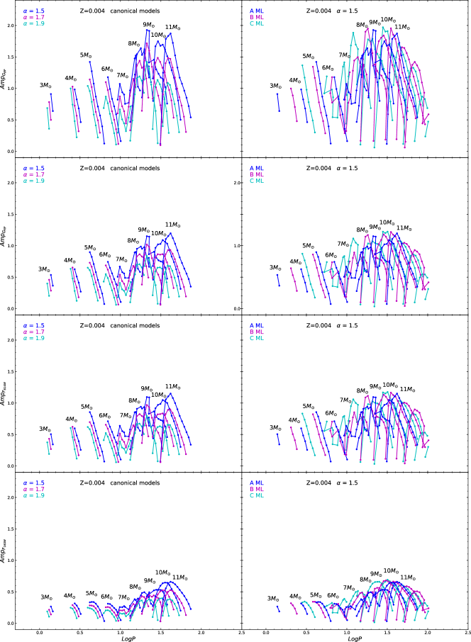
Figure 15: From top to bottom, the left panels show the F-mode canonical theoretical amplitudes (solid lines) in the $G_{BP}$ and $G_{RP}$ Gaia bands and the F814W and F160W HST-WFC3 bands for Z = 0.004 Y = 0.25, for various assumptions of the $\alpha_{ml}$ parameters, while the right panels show the same F-mode theoretical amplitudes for various assumptions about the ML relation at a fixed mixing length parameter $\alpha_{ml}=1.5$.

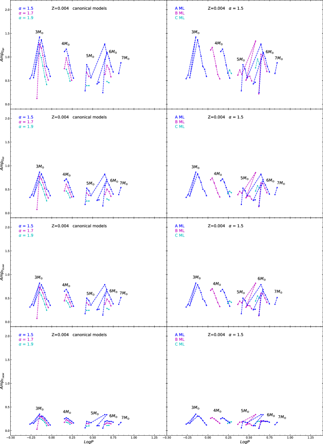
Figure 16: The same as Fig.15 but for the FO-mode models.

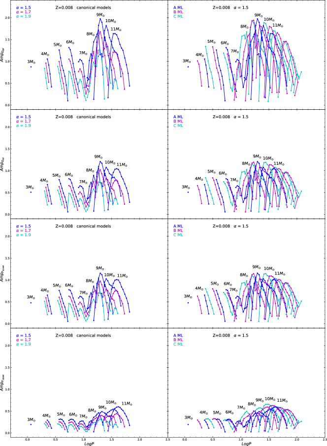
Figure 17: The same as Fig.15 but for Z=0.008 and Y=0.25.

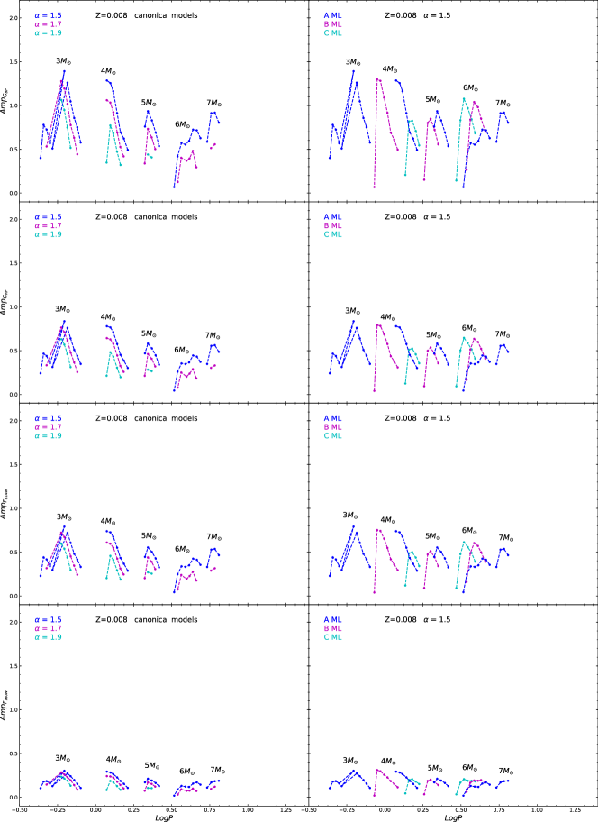
Figure 18: The same as Fig.16 but for Z=0.008 and Y=0.25.

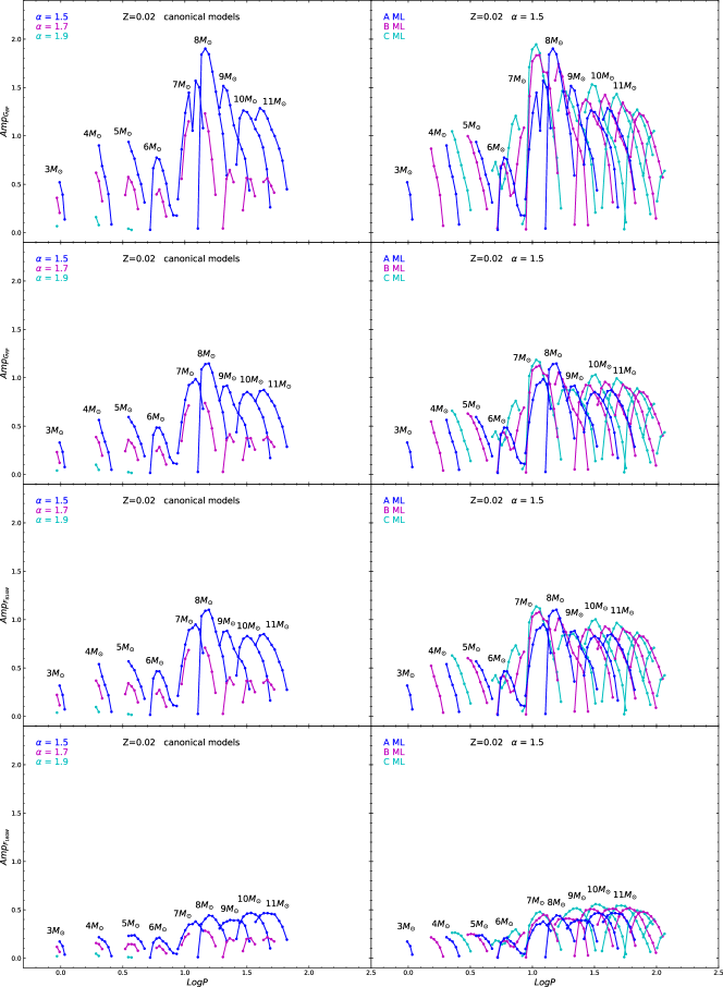
Figure 19: The same as Fig.15 but for Z=0.02 and Y=0.28.

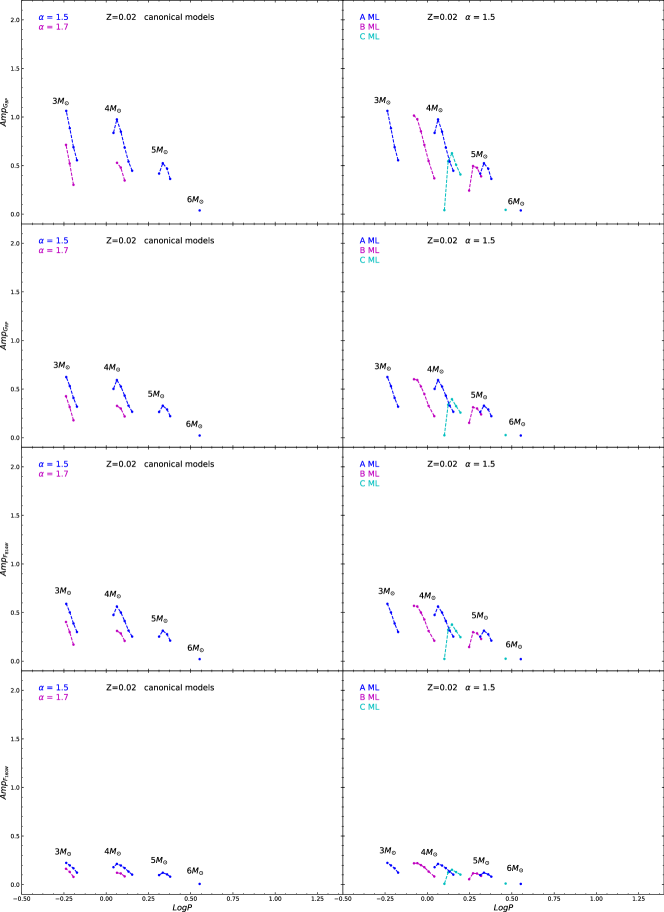
Figure 20: The same as Fig.16 but for Z=0.02 and Y=0.28.

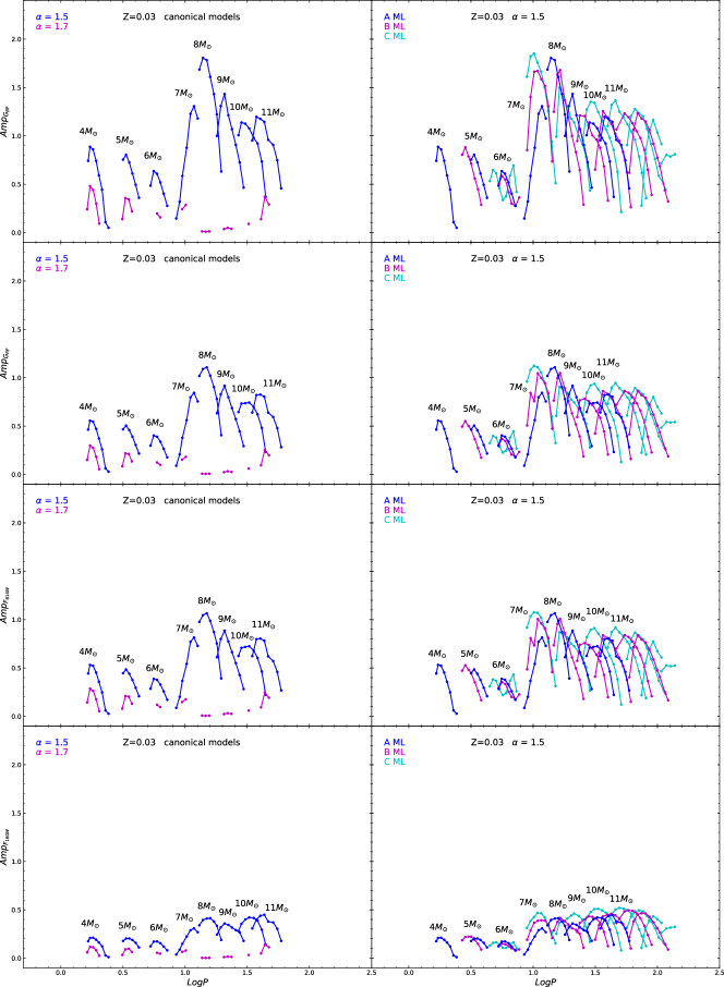
Figure 21: The same as Fig.15 but for Z=0.03 and Y=0.28.

B.1 The comparison between theoretical and observed pulsational amplitudes for Z=0.004 and Z=0.008 in the Gaia DR2 database

Figure 22: The comparison between theoretical F and FO-mode amplitudes (solid green lines and dashed blue lines, respectively) and Z=0.004 F and FO-mode data (green points and blue plus, respectively.) The upper panel and middle panels show the comparison for canonical ML relation with $\alpha_{ml}=1.5$ and $\alpha_{ml}=1.7$, respectively while the bottom panel shows the comparison for noncanonical ML relation (case B) with $\alpha_{ml}=1.5$.

Figure 23: The same as Fig.22 but for the $G_{RP}$ Gaia band.

Figure 24: The same as Fig.22 but for Z=0.008.

Figure 25: The same as Fig.24 but for the $G_{RP}$ Gaia band.

Appendix C PLC coefficients in the Gaia EDR3, HST-WFC3 and Johnson-Cousins filters

Table 28: PLC coefficients in the Gaia EDR3 filters ($<G>$=a+b$\log P$ +c($<G_{BP}>$ - $<G_{RP}>$) for F and FO CCs derived by adopting A, B, C ML relations and $\alpha_{ml}$ = 1.5, 1.7 and 1.9.

Z	Y	$\alpha_{ml}$	ML	a	b	c	$\sigma_{a}$	$\sigma_{b}$	$\sigma_{c}$	$\sigma$	$R^{2}$
F
0.004	0.25	1.5	A	-3.143	-3.741	3.107	0.019	0.013	0.033	0.029	0.999
0.004	0.25	1.7	A	-3.142	-3.757	3.121	0.019	0.012	0.035	0.023	1.000
0.004	0.25	1.9	A	-3.131	-3.781	3.132	0.022	0.013	0.043	0.019	1.000
0.004	0.25	1.5	B	-3.028	-3.709	3.112	0.024	0.017	0.041	0.043	0.999
0.004	0.25	1.7	B	-3.032	-3.731	3.153	0.017	0.012	0.032	0.026	1.000
0.004	0.25	1.9	B	-3.051	-3.756	3.211	0.019	0.013	0.039	0.023	1.000
0.004	0.25	1.5	C	-2.894	-3.683	3.100	0.030	0.017	0.047	0.046	0.999
0.004	0.25	1.7	C	-2.876	-3.689	3.098	0.021	0.013	0.037	0.031	0.999
0.004	0.25	1.9	C	-2.881	-3.710	3.136	0.021	0.014	0.041	0.026	1.000
0.008	0.25	1.5	A	-3.233	-3.785	3.082	0.020	0.016	0.035	0.031	0.999
0.008	0.25	1.7	A	-3.195	-3.785	3.021	0.023	0.018	0.045	0.023	0.999
0.008	0.25	1.9	A	-3.152	-3.830	3.009	0.030	0.022	0.060	0.017	1.000
0.008	0.25	1.5	B	-3.141	-3.765	3.136	0.023	0.018	0.040	0.043	0.999
0.008	0.25	1.7	B	-3.185	-3.812	3.246	0.025	0.021	0.050	0.037	0.999
0.008	0.25	1.9	B	-3.165	-3.849	3.261	0.039	0.031	0.081	0.032	0.999
0.008	0.25	1.5	C	-2.942	-3.718	3.033	0.024	0.016	0.039	0.039	0.999
0.008	0.25	1.7	C	-2.985	-3.735	3.099	0.023	0.016	0.042	0.033	0.999
0.008	0.25	1.9	C	-3.012	-3.765	3.169	0.039	0.032	0.082	0.039	0.999
0.02	0.28	1.5	A	-3.451	-3.854	3.233	0.037	0.028	0.062	0.039	0.999
0.02	0.28	1.7	A	-3.546	-4.007	3.475	0.084	0.062	0.151	0.033	0.999
0.02	0.28	1.9	A	-3.158	-3.850	2.860	0.058	0.025	0.097	0.002	1.000
0.02	0.28	1.5	B	-3.387	-3.816	3.298	0.037	0.029	0.062	0.049	0.998
0.02	0.28	1.7	B	-3.564	-3.961	3.630	0.088	0.070	0.159	0.060	0.998
0.02	0.28	1.9	B	-2.990	-3.831	2.828	0.040	0.020	0.067	0.002	1.000
0.02	0.28	1.5	C	-3.196	-3.744	3.182	0.034	0.024	0.053	0.048	0.998
0.02	0.28	1.7	C	-3.099	-3.712	3.041	0.069	0.051	0.121	0.055	0.998
0.02	0.28	1.9	C	-2.909	-3.920	2.980	0.038	0.030	0.073	0.004	1.000
0.03	0.28	1.5	A	-3.557	-3.853	3.215	0.050	0.038	0.082	0.040	0.999
0.03	0.28	1.7	A	-3.634	-3.978	3.388	0.221	0.166	0.376	0.045	0.999
FO
0.004	0.25	1.5	A	-3.691	-3.680	3.163	0.300	0.169	0.603	0.165	0.975
0.004	0.25	1.7	A	-3.549	-3.894	3.015	0.069	0.038	0.142	0.022	0.999
0.004	0.25	1.9	A	-3.509	-3.898	2.937	0.060	0.030	0.123	0.011	1.000
0.004	0.25	1.5	B	-3.173	-3.653	2.523	0.286	0.214	0.585	0.127	0.968
0.004	0.25	1.7	B	-3.105	-3.534	2.325	0.437	0.316	0.919	0.137	0.959
0.004	0.25	1.9	B	-3.396	-3.866	2.968	0.035	0.018	0.073	0.003	1.000
0.004	0.25	1.5	C	-3.199	-3.788	2.834	0.038	0.025	0.085	0.003	1.000
0.004	0.25	1.7	C	-3.489	-3.959	3.476	0.008	0.005	0.018	0.000	1.000
0.008	0.25	1.5	A	-3.818	-3.754	3.123	0.198	0.108	0.376	0.113	0.990
0.008	0.25	1.7	A	-3.622	-3.844	2.881	0.187	0.101	0.360	0.076	0.995
0.008	0.25	1.9	A	-3.599	-3.951	2.879	0.066	0.034	0.130	0.011	1.000
0.008	0.25	1.5	B	-3.475	-3.898	2.921	0.044	0.031	0.088	0.018	0.999
0.008	0.25	1.7	B	-3.432	-3.882	2.836	0.040	0.025	0.078	0.010	1.000
0.008	0.25	1.9	B	-3.450	-3.864	2.853	0.058	0.038	0.114	0.007	1.000
0.008	0.25	1.5	C	-3.355	-3.830	2.917	0.044	0.039	0.093	0.011	1.000
0.008	0.25	1.7	C	-3.411	-3.882	3.040	0.055	0.046	0.119	0.007	1.000
0.02	0.28	1.5	A	-3.610	-3.974	2.677	0.029	0.015	0.049	0.007	1.000
0.02	0.28	1.7	A	-3.661	-3.981	2.735	0.044	0.020	0.076	0.003	1.000

Table 28: continued.

Table 29: PLC coefficients in the HST-WFC3 filters ($<F_{160W}>$=a+b$\log P$ +c($<F_{555W}>$ - $<F_{814W}>$) for F and FO CCs derived by adopting A, B, C ML relations and $\alpha_{ml}$ = 1.5, 1.7 and 1.9.

Z	Y	$\alpha_{ml}$	ML	a	b	c	$\sigma_{a}$	$\sigma_{b}$	$\sigma_{c}$	$\sigma$	$R^{2}$
F
0.004	0.25	1.5	A	-3.190	-3.744	1.549	0.018	0.013	0.032	0.028	1.000
0.004	0.25	1.7	A	-3.187	-3.753	1.563	0.019	0.012	0.035	0.022	1.000
0.004	0.25	1.9	A	-3.175	-3.773	1.579	0.024	0.014	0.047	0.020	1.000
0.004	0.25	1.5	B	-3.083	-3.686	1.533	0.024	0.016	0.042	0.042	0.999
0.004	0.25	1.7	B	-3.088	-3.709	1.589	0.019	0.013	0.037	0.029	1.000
0.004	0.25	1.9	B	-3.106	-3.732	1.653	0.025	0.016	0.051	0.030	1.000
0.004	0.25	1.5	C	-2.948	-3.639	1.492	0.031	0.017	0.049	0.046	0.999
0.004	0.25	1.7	C	-2.926	-3.647	1.494	0.025	0.015	0.045	0.036	0.999
0.004	0.25	1.9	C	-2.932	-3.671	1.547	0.027	0.018	0.054	0.034	1.000
0.008	0.25	1.5	A	-3.224	-3.766	1.504	0.015	0.012	0.028	0.024	1.000
0.008	0.25	1.7	A	-3.214	-3.767	1.489	0.019	0.015	0.038	0.019	1.000
0.008	0.25	1.9	A	-3.184	-3.796	1.486	0.029	0.020	0.061	0.017	1.000
0.008	0.25	1.5	B	-3.119	-3.727	1.521	0.021	0.017	0.037	0.040	0.999
0.008	0.25	1.7	B	-3.173	-3.778	1.663	0.021	0.018	0.044	0.032	1.000
0.008	0.25	1.9	B	-3.175	-3.811	1.715	0.036	0.028	0.078	0.030	1.000
0.008	0.25	1.5	C	-2.930	-3.658	1.398	0.025	0.016	0.041	0.041	0.999
0.008	0.25	1.7	C	-2.967	-3.669	1.460	0.023	0.017	0.044	0.034	0.999
0.008	0.25	1.9	C	-2.998	-3.706	1.557	0.037	0.030	0.081	0.037	0.999
0.02	0.28	1.5	A	-3.305	-3.813	1.583	0.024	0.019	0.043	0.028	1.000
0.02	0.28	1.7	A	-3.416	-3.944	1.851	0.055	0.042	0.104	0.023	1.000
0.02	0.28	1.9	A	-3.088	-3.844	1.321	0.086	0.038	0.152	0.003	1.000
0.02	0.28	1.5	B	-3.214	-3.761	1.604	0.026	0.022	0.047	0.039	0.999
0.02	0.28	1.7	B	-3.353	-3.883	1.898	0.055	0.047	0.107	0.044	0.999
0.02	0.28	1.9	B	-2.912	-3.817	1.268	0.025	0.012	0.045	0.001	1.000
0.02	0.28	1.5	C	-3.020	-3.666	1.455	0.026	0.020	0.043	0.041	0.999
0.02	0.28	1.7	C	-2.963	-3.659	1.388	0.050	0.040	0.094	0.044	0.999
0.02	0.28	1.9	C	-2.811	-3.829	1.351	0.053	0.041	0.107	0.006	1.000
0.03	0.28	1.5	A	-3.353	-3.808	1.538	0.030	0.025	0.053	0.027	1.000
0.03	0.28	1.7	A	-3.469	-3.935	1.784	0.129	0.103	0.238	0.030	1.000
FO
0.004	0.25	1.5	A	-3.698	-3.690	1.570	0.283	0.159	0.581	0.157	0.982
0.004	0.25	1.7	A	-3.524	-3.888	1.358	0.044	0.024	0.092	0.014	1.000
0.004	0.25	1.9	A	-3.503	-3.899	1.328	0.043	0.022	0.090	0.008	1.000
0.004	0.25	1.5	B	-3.167	-3.659	0.889	0.275	0.205	0.573	0.122	0.977
0.004	0.25	1.7	B	-3.090	-3.542	0.682	0.419	0.303	0.899	0.133	0.971
0.004	0.25	1.9	B	-3.376	-3.868	1.335	0.010	0.005	0.020	0.001	1.000
0.004	0.25	1.5	C	-3.143	-3.800	1.132	0.030	0.020	0.069	0.003	1.000
0.004	0.25	1.7	C	-3.388	-3.950	1.699	0.049	0.031	0.111	0.002	1.000
0.008	0.25	1.5	A	-3.799	-3.754	1.562	0.179	0.097	0.354	0.104	0.993
0.008	0.25	1.7	A	-3.612	-3.840	1.332	0.172	0.093	0.344	0.071	0.996
0.008	0.25	1.9	A	-3.547	-3.928	1.256	0.039	0.021	0.081	0.007	1.000
0.008	0.25	1.5	B	-3.413	-3.871	1.261	0.018	0.012	0.036	0.007	1.000
0.008	0.25	1.7	B	-3.407	-3.872	1.253	0.020	0.012	0.040	0.005	1.000
0.008	0.25	1.9	B	-3.426	-3.852	1.287	0.046	0.031	0.094	0.006	1.000
0.008	0.25	1.5	C	-3.255	-3.817	1.203	0.018	0.016	0.039	0.004	1.000
0.008	0.25	1.7	C	-3.290	-3.858	1.295	0.028	0.024	0.064	0.004	1.000
0.02	0.28	1.5	A	-3.564	-3.949	1.155	0.025	0.013	0.046	0.006	1.000
0.02	0.28	1.7	A	-3.609	-3.979	1.224	0.029	0.013	0.053	0.002	1.000

Table 29: continued.

Table 30: PLC coefficients in the Johnson-Cousins filters ($<V>$=a+b$\log P$ +c($<V>$ - $<I>$) for F and FO CCs derived by adopting A, B, C ML relations and $\alpha_{ml}$ = 1.5, 1.7 and 1.9.

Z	Y	$\alpha_{ml}$	ML	a	b	c	$\sigma_{a}$	$\sigma_{b}$	$\sigma_{c}$	$\sigma$	$R^{2}$
F
0.004	0.25	1.5	A	-3.248	-3.727	3.830	0.019	0.013	0.037	0.029	0.999
0.004	0.25	1.7	A	-3.248	-3.743	3.851	0.020	0.013	0.042	0.024	1.000
0.004	0.25	1.9	A	-3.224	-3.767	3.849	0.026	0.015	0.056	0.022	1.000
0.004	0.25	1.5	B	-3.138	-3.690	3.839	0.024	0.016	0.045	0.042	0.999
0.004	0.25	1.7	B	-3.142	-3.713	3.889	0.019	0.012	0.039	0.028	0.999
0.004	0.25	1.9	B	-3.158	-3.739	3.955	0.023	0.015	0.052	0.028	1.000
0.004	0.25	1.5	C	-3.002	-3.660	3.816	0.030	0.017	0.053	0.045	0.999
0.004	0.25	1.7	C	-2.980	-3.667	3.814	0.023	0.014	0.045	0.033	0.999
0.004	0.25	1.9	C	-2.985	-3.690	3.861	0.025	0.016	0.054	0.031	0.999
0.008	0.25	1.5	A	-3.289	-3.763	3.781	0.018	0.014	0.036	0.028	0.999
0.008	0.25	1.7	A	-3.272	-3.763	3.746	0.023	0.017	0.049	0.023	0.999
0.008	0.25	1.9	A	-3.233	-3.805	3.740	0.033	0.023	0.076	0.019	1.000
0.008	0.25	1.5	B	-3.178	-3.733	3.805	0.021	0.017	0.041	0.041	0.999
0.008	0.25	1.7	B	-3.235	-3.783	3.956	0.021	0.018	0.048	0.032	0.999
0.008	0.25	1.9	B	-3.236	-3.822	4.011	0.038	0.030	0.090	0.032	0.999
0.008	0.25	1.5	C	-2.992	-3.682	3.701	0.024	0.016	0.043	0.039	0.999
0.008	0.25	1.7	C	-3.036	-3.697	3.780	0.022	0.015	0.044	0.032	0.999
0.008	0.25	1.9	C	-3.068	-3.729	3.872	0.037	0.030	0.088	0.037	0.999
0.02	0.28	1.5	A	-3.365	-3.809	3.811	0.024	0.019	0.047	0.028	0.999
0.02	0.28	1.7	A	-3.496	-3.961	4.141	0.059	0.045	0.124	0.026	1.000
0.02	0.28	1.9	A	-3.125	-3.827	3.468	0.071	0.031	0.137	0.002	1.000
0.02	0.28	1.5	B	-3.245	-3.755	3.797	0.022	0.019	0.043	0.034	0.999
0.02	0.28	1.7	B	-3.401	-3.880	4.132	0.051	0.045	0.110	0.043	0.999
0.02	0.28	1.9	B	-2.955	-3.805	3.426	0.030	0.015	0.059	0.002	1.000
0.02	0.28	1.5	C	-3.067	-3.681	3.679	0.023	0.018	0.040	0.037	0.999
0.02	0.28	1.7	C	-3.040	-3.679	3.642	0.050	0.040	0.102	0.045	0.999
0.02	0.28	1.9	C	-2.871	-3.861	3.574	0.051	0.039	0.111	0.005	1.000
0.03	0.28	1.5	A	-3.396	-3.796	3.710	0.030	0.025	0.057	0.028	0.999
0.03	0.28	1.7	A	-3.595	-3.987	4.133	0.142	0.115	0.288	0.034	0.999
FO
0.004	0.25	1.5	A	-3.700	-3.690	3.770	0.285	0.163	0.636	0.161	0.976
0.004	0.25	1.7	A	-3.502	-3.878	3.480	0.058	0.033	0.132	0.019	1.000
0.004	0.25	1.9	A	-3.462	-3.883	3.396	0.066	0.034	0.151	0.013	1.000
0.004	0.25	1.5	B	-3.169	-3.652	3.027	0.278	0.210	0.629	0.125	0.968
0.004	0.25	1.7	B	-3.096	-3.536	2.801	0.420	0.310	0.982	0.136	0.958
0.004	0.25	1.9	B	-3.331	-3.842	3.387	0.046	0.024	0.106	0.004	1.000
0.004	0.25	1.5	C	-3.166	-3.780	3.311	0.028	0.019	0.069	0.002	1.000
0.004	0.25	1.7	C	-3.398	-3.924	3.887	0.019	0.012	0.046	0.001	1.000
0.008	0.25	1.5	A	-3.812	-3.754	3.757	0.181	0.099	0.388	0.107	0.991
0.008	0.25	1.7	A	-3.608	-3.835	3.462	0.175	0.095	0.379	0.073	0.995
0.008	0.25	1.9	A	-3.526	-3.929	3.332	0.058	0.031	0.129	0.011	1.000
0.008	0.25	1.5	B	-3.430	-3.870	3.434	0.036	0.026	0.082	0.015	1.000
0.008	0.25	1.7	B	-3.388	-3.855	3.342	0.040	0.025	0.090	0.010	1.000
0.008	0.25	1.9	B	-3.375	-3.837	3.296	0.055	0.038	0.124	0.007	1.000
0.008	0.25	1.5	C	-3.312	-3.810	3.441	0.032	0.029	0.078	0.008	1.000
0.008	0.25	1.7	C	-3.355	-3.862	3.555	0.037	0.032	0.092	0.005	1.000
0.02	0.28	1.5	A	-3.546	-3.943	3.207	0.028	0.015	0.056	0.007	1.000
0.02	0.28	1.7	A	-3.572	-3.956	3.227	0.045	0.021	0.090	0.003	1.000

Table 30: continued.

Table 31: PLC coefficients in the Johnson-Cousins filters ($<V>$=a+b$\log P$ +c($<V>$ - $<K>$) for F and FO CCs derived by adopting A, B, C ML relations and $\alpha_{ml}$ = 1.5, 1.7 and 1.9.

Z	Y	$\alpha_{ml}$	ML	a	b	c	$\sigma_{a}$	$\sigma_{b}$	$\sigma_{c}$	$\sigma$	$R^{2}$
F
0.004	0.25	1.5	A	-3.099	-3.772	1.667	0.018	0.014	0.016	0.029	0.999
0.004	0.25	1.7	A	-3.099	-3.774	1.675	0.019	0.013	0.018	0.024	1.000
0.004	0.25	1.9	A	-3.094	-3.790	1.689	0.024	0.015	0.024	0.022	1.000
0.004	0.25	1.5	B	-2.997	-3.686	1.644	0.026	0.018	0.022	0.047	0.998
0.004	0.25	1.7	B	-3.006	-3.710	1.678	0.022	0.016	0.022	0.036	0.999
0.004	0.25	1.9	B	-3.021	-3.728	1.708	0.028	0.020	0.029	0.036	0.999
0.004	0.25	1.5	C	-2.866	-3.622	1.614	0.033	0.019	0.025	0.052	0.998
0.004	0.25	1.7	C	-2.844	-3.628	1.617	0.029	0.018	0.025	0.044	0.999
0.004	0.25	1.9	C	-2.849	-3.653	1.646	0.031	0.021	0.031	0.041	0.999
0.008	0.25	1.5	A	-3.101	-3.777	1.626	0.013	0.011	0.012	0.021	1.000
0.008	0.25	1.7	A	-3.122	-3.783	1.645	0.017	0.014	0.017	0.018	1.000
0.008	0.25	1.9	A	-3.105	-3.795	1.647	0.029	0.022	0.031	0.018	1.000
0.008	0.25	1.5	B	-2.984	-3.720	1.615	0.020	0.017	0.018	0.042	0.999
0.008	0.25	1.7	B	-3.044	-3.771	1.693	0.019	0.017	0.020	0.031	0.999
0.008	0.25	1.9	B	-3.069	-3.798	1.735	0.033	0.028	0.038	0.031	0.999
0.008	0.25	1.5	C	-2.808	-3.627	1.547	0.026	0.018	0.021	0.047	0.999
0.008	0.25	1.7	C	-2.845	-3.633	1.577	0.025	0.018	0.023	0.039	0.999
0.008	0.25	1.9	C	-2.877	-3.668	1.628	0.034	0.030	0.038	0.039	0.999
0.02	0.28	1.5	A	-3.071	-3.798	1.605	0.017	0.015	0.016	0.023	1.000
0.02	0.28	1.7	A	-3.164	-3.879	1.712	0.033	0.029	0.034	0.017	1.000
0.02	0.28	1.9	A	-3.010	-3.863	1.595	0.097	0.047	0.091	0.003	1.000
0.02	0.28	1.5	B	-2.963	-3.734	1.598	0.020	0.019	0.019	0.035	0.999
0.02	0.28	1.7	B	-3.039	-3.808	1.691	0.032	0.032	0.034	0.032	0.999
0.02	0.28	1.9	B	-2.836	-3.834	1.568	0.019	0.010	0.018	0.001	1.000
0.02	0.28	1.5	C	-2.778	-3.617	1.515	0.023	0.019	0.019	0.041	0.999
0.02	0.28	1.7	C	-2.742	-3.618	1.502	0.035	0.031	0.034	0.037	0.999
0.02	0.28	1.9	C	-2.707	-3.805	1.576	0.047	0.038	0.050	0.005	1.000
0.03	0.28	1.5	A	-3.090	-3.794	1.577	0.018	0.018	0.017	0.020	1.000
0.03	0.28	1.7	A	-3.176	-3.864	1.668	0.041	0.039	0.042	0.013	1.000
FO
0.004	0.25	1.5	A	-3.739	-3.748	1.798	0.266	0.158	0.277	0.152	0.978
0.004	0.25	1.7	A	-3.514	-3.914	1.640	0.031	0.018	0.033	0.010	1.000
0.004	0.25	1.9	A	-3.511	-3.929	1.646	0.030	0.016	0.032	0.006	1.000
0.004	0.25	1.5	B	-3.179	-3.698	1.424	0.262	0.206	0.277	0.120	0.970
0.004	0.25	1.7	B	-3.127	-3.594	1.350	0.400	0.307	0.438	0.132	0.961
0.004	0.25	1.9	B	-3.375	-3.902	1.645	0.021	0.011	0.023	0.002	1.000
0.004	0.25	1.5	C	-3.096	-3.824	1.491	0.041	0.030	0.048	0.004	1.000
0.004	0.25	1.7	C	-3.328	-3.987	1.775	0.080	0.057	0.094	0.003	1.000
0.008	0.25	1.5	A	-3.792	-3.788	1.756	0.166	0.095	0.168	0.101	0.992
0.008	0.25	1.7	A	-3.613	-3.868	1.648	0.163	0.092	0.168	0.069	0.996
0.008	0.25	1.9	A	-3.534	-3.939	1.600	0.028	0.015	0.029	0.005	1.000
0.008	0.25	1.5	B	-3.365	-3.880	1.559	0.012	0.009	0.013	0.005	1.000
0.008	0.25	1.7	B	-3.389	-3.894	1.589	0.018	0.011	0.019	0.005	1.000
0.008	0.25	1.9	B	-3.437	-3.873	1.640	0.041	0.027	0.044	0.005	1.000
0.008	0.25	1.5	C	-3.178	-3.828	1.505	0.021	0.021	0.024	0.006	1.000
0.008	0.25	1.7	C	-3.203	-3.858	1.542	0.033	0.031	0.039	0.005	1.000
0.02	0.28	1.5	A	-3.543	-3.959	1.549	0.028	0.015	0.027	0.007	1.000
0.02	0.28	1.7	A	-3.604	-4.008	1.610	0.031	0.015	0.030	0.002	1.000

Table 31: continued.

Appendix D PW coefficients in the Gaia EDR3, HST-WFC3 and Johnson-Cousins filters

Table 32: PW coefficients in the Gaia EDR3 filters ($<W>=<G>-1.9<G_{BP}-G_{RP}>=a+b\log P$) for F and FO CCs derived by adopting A, B, C ML relations and $\alpha_{ml}$ = 1.5, 1.7 and 1.9.

Z	Y	$\alpha_{ml}$	ML	a	b	$\sigma_{a}$	$\sigma_{b}$	$\sigma$	$R^{2}$
F
0.004	0.25	1.5	A	-2.580	-3.350	0.045	0.034	0.123	0.992
0.004	0.25	1.7	A	-2.559	-3.403	0.039	0.031	0.102	0.995
0.004	0.25	1.9	A	-2.540	-3.453	0.030	0.026	0.078	0.997
0.004	0.25	1.5	B	-2.471	-3.318	0.048	0.033	0.137	0.991
0.004	0.25	1.7	B	-2.474	-3.336	0.039	0.028	0.114	0.994
0.004	0.25	1.9	B	-2.472	-3.360	0.034	0.024	0.098	0.996
0.004	0.25	1.5	C	-2.272	-3.365	0.051	0.035	0.136	0.991
0.004	0.25	1.7	C	-2.319	-3.340	0.043	0.029	0.117	0.994
0.004	0.25	1.9	C	-2.333	-3.340	0.039	0.026	0.100	0.996
0.008	0.25	1.5	A	-2.670	-3.341	0.044	0.036	0.122	0.991
0.008	0.25	1.7	A	-2.668	-3.384	0.037	0.031	0.082	0.996
0.008	0.25	1.9	A	-2.634	-3.460	0.027	0.025	0.055	0.998
0.008	0.25	1.5	B	-2.581	-3.281	0.046	0.032	0.143	0.991
0.008	0.25	1.7	B	-2.596	-3.287	0.039	0.028	0.120	0.994
0.008	0.25	1.9	B	-2.555	-3.358	0.031	0.024	0.082	0.997
0.008	0.25	1.5	C	-2.365	-3.339	0.044	0.030	0.127	0.993
0.008	0.25	1.7	C	-2.419	-3.321	0.041	0.027	0.112	0.995
0.008	0.25	1.9	C	-2.460	-3.296	0.033	0.023	0.088	0.997
0.02	0.28	1.5	A	-2.698	-3.300	0.035	0.029	0.110	0.995
0.02	0.28	1.7	A	-2.677	-3.370	0.028	0.025	0.070	0.998
0.02	0.28	1.9	A	-2.582	-3.605	0.014	0.034	0.013	1.000
0.02	0.28	1.5	B	-2.636	-3.205	0.041	0.029	0.132	0.993
0.02	0.28	1.7	B	-2.641	-3.218	0.039	0.028	0.110	0.996
0.02	0.28	1.9	B	-2.439	-3.585	0.028	0.069	0.020	0.999
0.02	0.28	1.5	C	-2.476	-3.225	0.049	0.034	0.142	0.992
0.02	0.28	1.7	C	-2.479	-3.249	0.036	0.026	0.092	0.997
0.02	0.28	1.9	C	-2.342	-3.493	0.028	0.045	0.026	0.999
0.03	0.28	1.5	A	-2.779	-3.264	0.032	0.028	0.095	0.996
0.03	0.28	1.7	A	-2.764	-3.326	0.028	0.027	0.061	0.999
FO
0.004	0.25	1.5	A	-3.069	-3.378	0.043	0.092	0.177	0.978
0.004	0.25	1.7	A	-3.011	-3.629	0.015	0.041	0.050	0.998
0.004	0.25	1.9	A	-3.005	-3.665	0.013	0.035	0.033	0.999
0.004	0.25	1.5	B	-2.876	-3.477	0.063	0.136	0.131	0.975
0.004	0.25	1.7	B	-2.906	-3.411	0.073	0.167	0.138	0.970
0.004	0.25	1.9	B	-2.878	-3.631	0.020	0.061	0.028	0.999
0.004	0.25	1.5	C	-2.783	-3.536	0.027	0.059	0.020	0.999
0.004	0.25	1.7	C	-2.778	-3.545	0.049	0.130	0.027	0.997
0.008	0.25	1.5	A	-3.178	-3.451	0.027	0.061	0.131	0.990
0.008	0.25	1.7	A	-3.114	-3.600	0.022	0.054	0.088	0.995
0.008	0.25	1.9	A	-3.104	-3.740	0.011	0.053	0.032	0.998
0.008	0.25	1.5	B	-2.966	-3.603	0.020	0.053	0.056	0.996
0.008	0.25	1.7	B	-2.959	-3.627	0.017	0.045	0.039	0.998
0.008	0.25	1.9	B	-2.971	-3.621	0.016	0.095	0.032	0.997
0.008	0.25	1.5	C	-2.887	-3.474	0.032	0.078	0.042	0.995
0.008	0.25	1.7	C	-2.892	-3.478	0.027	0.069	0.031	0.998
0.02	0.28	1.5	A	-3.155	-3.775	0.010	0.037	0.031	0.999
0.02	0.28	1.7	A	-3.179	-3.808	0.011	0.066	0.020	0.999

Table 32: continued.

Table 33: PW coefficients in the HST-WFC3 filters ($<W>=<F_{160W}>-0.386<F_{555W}-F_{814W}>=a+b\log P$) for F and FO CCs derived by adopting A, B, C ML relations and $\alpha_{ml}$ = 1.5, 1.7 and 1.9.

Z	Y	$\alpha_{ml}$	ML	a	b	$\sigma_{a}$	$\sigma_{b}$	$\sigma$	$R^{2}$
F
0.004	0.25	1.5	A	-2.652	-3.385	0.042	0.032	0.115	0.993
0.004	0.25	1.7	A	-2.629	-3.431	0.036	0.029	0.095	0.995
0.004	0.25	1.9	A	-2.607	-3.475	0.028	0.024	0.073	0.997
0.004	0.25	1.5	B	-2.561	-3.334	0.044	0.031	0.127	0.992
0.004	0.25	1.7	B	-2.556	-3.351	0.037	0.026	0.108	0.995
0.004	0.25	1.9	B	-2.550	-3.371	0.033	0.023	0.094	0.997
0.004	0.25	1.5	C	-2.381	-3.364	0.047	0.032	0.124	0.992
0.004	0.25	1.7	C	-2.415	-3.342	0.040	0.027	0.108	0.995
0.004	0.25	1.9	C	-2.420	-3.344	0.036	0.025	0.094	0.996
0.008	0.25	1.5	A	-2.712	-3.364	0.041	0.033	0.112	0.993
0.008	0.25	1.7	A	-2.713	-3.395	0.035	0.029	0.078	0.996
0.008	0.25	1.9	A	-2.682	-3.456	0.026	0.024	0.052	0.998
0.008	0.25	1.5	B	-2.628	-3.299	0.042	0.030	0.131	0.992
0.008	0.25	1.7	B	-2.637	-3.302	0.037	0.027	0.112	0.995
0.008	0.25	1.9	B	-2.599	-3.359	0.030	0.023	0.079	0.998
0.008	0.25	1.5	C	-2.435	-3.336	0.040	0.027	0.114	0.994
0.008	0.25	1.7	C	-2.478	-3.317	0.036	0.025	0.101	0.996
0.008	0.25	1.9	C	-2.507	-3.295	0.031	0.021	0.081	0.998
0.02	0.28	1.5	A	-2.679	-3.323	0.032	0.026	0.100	0.996
0.02	0.28	1.7	A	-2.661	-3.372	0.026	0.023	0.064	0.999
0.02	0.28	1.9	A	-2.559	-3.621	0.013	0.033	0.012	1.000
0.02	0.28	1.5	B	-2.619	-3.227	0.037	0.026	0.119	0.995
0.02	0.28	1.7	B	-2.616	-3.236	0.035	0.025	0.098	0.997
0.02	0.28	1.9	B	-2.417	-3.599	0.026	0.063	0.018	0.999
0.02	0.28	1.5	C	-2.471	-3.234	0.043	0.029	0.124	0.994
0.02	0.28	1.7	C	-2.462	-3.257	0.031	0.022	0.080	0.998
0.02	0.28	1.9	C	-2.332	-3.471	0.025	0.040	0.023	0.999
0.03	0.28	1.5	A	-2.730	-3.290	0.029	0.025	0.085	0.997
0.03	0.28	1.7	A	-2.716	-3.332	0.023	0.022	0.049	0.999
FO
0.004	0.25	1.5	A	-3.127	-3.415	0.041	0.087	0.168	0.981
0.004	0.25	1.7	A	-3.064	-3.662	0.013	0.034	0.042	0.999
0.004	0.25	1.9	A	-3.056	-3.693	0.011	0.031	0.029	0.999
0.004	0.25	1.5	B	-2.932	-3.521	0.060	0.130	0.125	0.977
0.004	0.25	1.7	B	-2.954	-3.459	0.071	0.162	0.134	0.972
0.004	0.25	1.9	B	-2.925	-3.665	0.018	0.054	0.024	0.999
0.004	0.25	1.5	C	-2.818	-3.605	0.022	0.047	0.016	0.999
0.004	0.25	1.7	C	-2.809	-3.613	0.042	0.110	0.023	0.998
0.008	0.25	1.5	A	-3.207	-3.475	0.025	0.056	0.121	0.991
0.008	0.25	1.7	A	-3.141	-3.617	0.021	0.051	0.082	0.996
0.008	0.25	1.9	A	-3.123	-3.747	0.009	0.045	0.028	0.999
0.008	0.25	1.5	B	-2.993	-3.630	0.016	0.043	0.045	0.998
0.008	0.25	1.7	B	-2.986	-3.647	0.015	0.040	0.034	0.999
0.008	0.25	1.9	B	-2.991	-3.631	0.015	0.089	0.030	0.997
0.008	0.25	1.5	C	-2.894	-3.543	0.025	0.060	0.032	0.997
0.008	0.25	1.7	C	-2.894	-3.547	0.021	0.053	0.024	0.999
0.02	0.28	1.5	A	-3.140	-3.764	0.009	0.035	0.030	0.999
0.02	0.28	1.7	A	-3.154	-3.815	0.011	0.064	0.020	0.999

Table 33: continued.

Table 34: PW coefficients in the Johnson-Cousins filters ($<W>=<I>-1.55<V-I>=a+b\log P$) for F and FO CCs derived by adopting A, B, C ML relations and $\alpha_{ml}$ = 1.5, 1.7 and 1.9.

Z	Y	$\alpha_{ml}$	ML	a	b	$\sigma_{a}$	$\sigma_{b}$	$\sigma$	$R^{2}$
F
0.004	0.25	1.5	A	-2.700	-3.364	0.042	0.032	0.117	0.993
0.004	0.25	1.7	A	-2.676	-3.416	0.037	0.029	0.097	0.995
0.004	0.25	1.9	A	-2.652	-3.467	0.029	0.024	0.074	0.997
0.004	0.25	1.5	B	-2.593	-3.328	0.046	0.031	0.131	0.992
0.004	0.25	1.7	B	-2.591	-3.348	0.038	0.026	0.109	0.995
0.004	0.25	1.9	B	-2.585	-3.372	0.033	0.024	0.094	0.997
0.004	0.25	1.5	C	-2.398	-3.371	0.049	0.034	0.129	0.992
0.004	0.25	1.7	C	-2.437	-3.349	0.041	0.028	0.111	0.995
0.004	0.25	1.9	C	-2.447	-3.352	0.037	0.025	0.096	0.996
0.008	0.25	1.5	A	-2.768	-3.356	0.042	0.033	0.115	0.992
0.008	0.25	1.7	A	-2.769	-3.393	0.035	0.029	0.078	0.996
0.008	0.25	1.9	A	-2.732	-3.467	0.026	0.024	0.053	0.998
0.008	0.25	1.5	B	-2.676	-3.298	0.043	0.030	0.134	0.992
0.008	0.25	1.7	B	-2.690	-3.302	0.037	0.027	0.113	0.995
0.008	0.25	1.9	B	-2.650	-3.367	0.030	0.023	0.080	0.998
0.008	0.25	1.5	C	-2.469	-3.347	0.041	0.028	0.119	0.994
0.008	0.25	1.7	C	-2.518	-3.329	0.038	0.026	0.105	0.995
0.008	0.25	1.9	C	-2.554	-3.306	0.032	0.022	0.084	0.998
0.02	0.28	1.5	A	-2.763	-3.332	0.031	0.026	0.098	0.996
0.02	0.28	1.7	A	-2.745	-3.391	0.027	0.024	0.066	0.998
0.02	0.28	1.9	A	-2.649	-3.626	0.012	0.030	0.011	1.000
0.02	0.28	1.5	B	-2.690	-3.247	0.035	0.025	0.115	0.995
0.02	0.28	1.7	B	-2.697	-3.254	0.035	0.024	0.097	0.997
0.02	0.28	1.9	B	-2.506	-3.605	0.024	0.059	0.017	0.999
0.02	0.28	1.5	C	-2.537	-3.258	0.042	0.029	0.123	0.994
0.02	0.28	1.7	C	-2.540	-3.276	0.032	0.023	0.082	0.998
0.02	0.28	1.9	C	-2.406	-3.512	0.025	0.039	0.023	0.999
0.03	0.28	1.5	A	-2.827	-3.311	0.028	0.024	0.082	0.997
0.03	0.28	1.7	A	-2.818	-3.359	0.025	0.024	0.054	0.999
FO
0.004	0.25	1.5	A	-3.158	-3.424	0.042	0.089	0.170	0.980
0.004	0.25	1.7	A	-3.097	-3.676	0.012	0.032	0.040	0.999
0.004	0.25	1.9	A	-3.093	-3.710	0.010	0.029	0.027	0.999
0.004	0.25	1.5	B	-2.964	-3.530	0.061	0.132	0.127	0.977
0.004	0.25	1.7	B	-2.990	-3.470	0.072	0.165	0.137	0.971
0.004	0.25	1.9	B	-2.965	-3.674	0.015	0.046	0.021	0.999
0.004	0.25	1.5	C	-2.861	-3.592	0.021	0.044	0.015	0.999
0.004	0.25	1.7	C	-2.857	-3.601	0.040	0.105	0.022	0.998
0.008	0.25	1.5	A	-3.255	-3.488	0.025	0.057	0.122	0.991
0.008	0.25	1.7	A	-3.191	-3.635	0.021	0.051	0.082	0.996
0.008	0.25	1.9	A	-3.177	-3.778	0.008	0.041	0.025	0.999
0.008	0.25	1.5	B	-3.040	-3.644	0.016	0.042	0.045	0.998
0.008	0.25	1.7	B	-3.035	-3.664	0.013	0.036	0.031	0.999
0.008	0.25	1.9	B	-3.044	-3.666	0.012	0.071	0.024	0.998
0.008	0.25	1.5	C	-2.951	-3.531	0.026	0.063	0.034	0.997
0.008	0.25	1.7	C	-2.954	-3.541	0.022	0.056	0.025	0.999
0.02	0.28	1.5	A	-3.215	-3.799	0.008	0.029	0.024	0.999
0.02	0.28	1.7	A	-3.237	-3.834	0.008	0.049	0.015	0.999

Table 34: continued.

Table 35: PW coefficients in the Johnson-Cousins filters ($<W>=<K>-0.13<V-K>=a+b\log P$) for F and FO CCs derived by adopting A, B, C ML relations and $\alpha_{ml}$ = 1.5, 1.7 and 1.9.

Z	Y	$\alpha_{ml}$	ML	a	b	$\sigma_{a}$	$\sigma_{b}$	$\sigma$	$R^{2}$
F
0.004	0.25	1.5	A	-2.618	-3.407	0.041	0.031	0.113	0.993
0.004	0.25	1.7	A	-2.597	-3.449	0.036	0.028	0.094	0.996
0.004	0.25	1.9	A	-2.576	-3.489	0.028	0.024	0.072	0.998
0.004	0.25	1.5	B	-2.533	-3.350	0.043	0.030	0.124	0.993
0.004	0.25	1.7	B	-2.528	-3.365	0.037	0.026	0.106	0.995
0.004	0.25	1.9	B	-2.522	-3.382	0.033	0.023	0.093	0.997
0.004	0.25	1.5	C	-2.361	-3.373	0.046	0.031	0.121	0.993
0.004	0.25	1.7	C	-2.392	-3.351	0.039	0.026	0.106	0.995
0.004	0.25	1.9	C	-2.395	-3.352	0.036	0.024	0.093	0.996
0.008	0.25	1.5	A	-2.670	-3.392	0.039	0.031	0.107	0.994
0.008	0.25	1.7	A	-2.676	-3.414	0.034	0.028	0.076	0.996
0.008	0.25	1.9	A	-2.651	-3.465	0.026	0.023	0.052	0.998
0.008	0.25	1.5	B	-2.585	-3.327	0.040	0.028	0.123	0.993
0.008	0.25	1.7	B	-2.597	-3.325	0.035	0.025	0.107	0.996
0.008	0.25	1.9	B	-2.566	-3.370	0.029	0.022	0.077	0.998
0.008	0.25	1.5	C	-2.405	-3.352	0.037	0.025	0.107	0.995
0.008	0.25	1.7	C	-2.448	-3.330	0.035	0.023	0.095	0.996
0.008	0.25	1.9	C	-2.475	-3.307	0.030	0.020	0.077	0.998
0.02	0.28	1.5	A	-2.619	-3.375	0.028	0.023	0.087	0.997
0.02	0.28	1.7	A	-2.612	-3.402	0.023	0.020	0.057	0.999
0.02	0.28	1.9	A	-2.519	-3.630	0.013	0.033	0.013	1.000
0.02	0.28	1.5	B	-2.551	-3.287	0.032	0.023	0.104	0.996
0.02	0.28	1.7	B	-2.549	-3.289	0.029	0.021	0.083	0.998
0.02	0.28	1.9	B	-2.378	-3.608	0.026	0.064	0.018	0.999
0.02	0.28	1.5	C	-2.412	-3.283	0.036	0.025	0.105	0.996
0.02	0.28	1.7	C	-2.403	-3.300	0.027	0.019	0.068	0.998
0.02	0.28	1.9	C	-2.294	-3.476	0.024	0.039	0.023	0.999
0.03	0.28	1.5	A	-2.661	-3.356	0.025	0.021	0.073	0.998
0.03	0.28	1.7	A	-2.657	-3.375	0.018	0.018	0.039	0.999
FO
0.004	0.25	1.5	A	-3.103	-3.422	0.041	0.087	0.167	0.981
0.004	0.25	1.7	A	-3.040	-3.668	0.013	0.034	0.043	0.999
0.004	0.25	1.9	A	-3.031	-3.698	0.012	0.033	0.031	0.999
0.004	0.25	1.5	B	-2.908	-3.528	0.060	0.129	0.124	0.978
0.004	0.25	1.7	B	-2.930	-3.465	0.070	0.161	0.133	0.973
0.004	0.25	1.9	B	-2.898	-3.671	0.019	0.057	0.026	0.999
0.004	0.25	1.5	C	-2.792	-3.616	0.022	0.047	0.016	0.999
0.004	0.25	1.7	C	-2.782	-3.624	0.043	0.112	0.023	0.998
0.008	0.25	1.5	A	-3.180	-3.480	0.025	0.056	0.121	0.991
0.008	0.25	1.7	A	-3.113	-3.619	0.021	0.051	0.082	0.995
0.008	0.25	1.9	A	-3.094	-3.747	0.010	0.047	0.029	0.999
0.008	0.25	1.5	B	-2.966	-3.636	0.016	0.043	0.045	0.998
0.008	0.25	1.7	B	-2.958	-3.651	0.015	0.042	0.036	0.999
0.008	0.25	1.9	B	-2.962	-3.627	0.016	0.094	0.031	0.997
0.008	0.25	1.5	C	-2.864	-3.555	0.025	0.060	0.032	0.997
0.008	0.25	1.7	C	-2.864	-3.556	0.021	0.053	0.024	0.999
0.02	0.28	1.5	A	-3.107	-3.764	0.010	0.037	0.032	0.999
0.02	0.28	1.7	A	-3.118	-3.819	0.011	0.069	0.021	0.999

Table 35: continued.

References

- Anderson et al. (2016) Anderson, R. I., Saio, H., Ekström, S., Georgy, C., & Meynet, G. 2016, A&A, 591, A8, doi: 10.1051/0004-6361/201528031
- Bono et al. (1997) Bono, G., Caputo, F., Cassisi, S., Castellani, V., & Marconi, M. 1997, apj, 489, 822, doi: 10.1086/304807
- Bono et al. (1999) Bono, G., Caputo, F., Castellani, V., & Marconi, M. 1999, ApJ, 512, 711, doi: 10.1086/306815
- Bono et al. (1998) Bono, G., Caputo, F., & Marconi, M. 1998, ApJ, 497, L43, doi: 10.1086/311270
- Bono et al. (2010) Bono, G., Caputo, F., Marconi, M., & Musella, I. 2010, ApJ, 715, 277, doi: 10.1088/0004-637X/715/1/277
- Bono et al. (2000a) Bono, G., Castellani, V., & Marconi, M. 2000a, ApJ, 529, 293, doi: 10.1086/308263
- Bono et al. (2000b) Bono, G., Marconi, M., & Stellingwerf, R. F. 2000b, A&A, 360, 245. https://arxiv.org/abs/astro-ph/0006229
- Breuval et al. (2021) Breuval, L., Kervella, P., Wielgórski, P., et al. 2021, ApJ, 913, 38, doi: 10.3847/1538-4357/abf0ae
- Caputo et al. (2005) Caputo, F., Bono, G., Fiorentino, G., Marconi, M., & Musella, I. 2005, ApJ, 629, 1021, doi: 10.1086/431641
- Carini et al. (2017) Carini, R., Brocato, E., Raimondo, G., & Marconi, M. 2017, MNRAS, 469, 1532, doi: 10.1093/mnras/stx927
- Chen et al. (2019) Chen, Y., Girardi, L., Fu, X., et al. 2019, A&A, 632, A105, doi: 10.1051/0004-6361/201936612
- De Somma et al. (2020a) De Somma, G., Marconi, M., Cassisi, S., et al. 2020a, MNRAS, 496, 5039, doi: 10.1093/mnras/staa1834
- De Somma et al. (2021a) —. 2021a, MNRAS, 508, 1473, doi: 10.1093/mnras/stab2611
- De Somma et al. (2020b) De Somma, G., Marconi, M., Molinaro, R., et al. 2020b, ApJS, 247, 30, doi: 10.3847/1538-4365/ab7204
- De Somma et al. (2021b) De Somma, G., Marconi, M., Molinaro, R., et al. 2021b, in Astronomical Society of the Pacific Conference Series, Vol. 529, RR Lyrae/Cepheid 2019: Frontiers of Classical Pulsators, ed. K. Kinemuchi, C. Lovekin, H. Neilson, & K. Vivas, 27
- Di Criscienzo et al. (2004) Di Criscienzo, M., Marconi, M., & Caputo, F. 2004, ApJ, 612, 1092, doi: 10.1086/422742
- Fausnaugh et al. (2015) Fausnaugh, M. M., Kochanek, C. S., Gerke, J. R., et al. 2015, MNRAS, 450, 3597, doi: 10.1093/mnras/stv881
- Fiorentino et al. (2007) Fiorentino, G., Marconi, M., Musella, I., & Caputo, F. 2007, A&A, 476, 863, doi: 10.1051/0004-6361:20077587
- Freedman & Madore (2011) Freedman, W. L., & Madore, B. F. 2011, ApJ, 734, 46, doi: 10.1088/0004-637X/734/1/46
- Gaia Collaboration et al. (2018) Gaia Collaboration, Brown, A. G. A., Vallenari, A., et al. 2018, A&A, 616, A1, doi: 10.1051/0004-6361/201833051
- Gaia Collaboration et al. (2021) —. 2021, A&A, 650, C3, doi: 10.1051/0004-6361/202039657e
- Graczyk et al. (2020) Graczyk, D., Pietrzyński, G., Thompson, I. B., et al. 2020, ApJ, 904, 13, doi: 10.3847/1538-4357/abbb2b
- Groenewegen (2013) Groenewegen, M. A. T. 2013, A&A, 550, A70, doi: 10.1051/0004-6361/201220446
- Hertzsprung (1926) Hertzsprung, E. 1926, Bull. Astron. Inst. Netherlands, 3, 115
- Hidalgo et al. (2018) Hidalgo, S. L., Pietrinferni, A., Cassisi, S., et al. 2018, ApJ, 856, 125, doi: 10.3847/1538-4357/aab158
- Kennicutt et al. (1998) Kennicutt, Robert C., J., Stetson, P. B., Saha, A., et al. 1998, ApJ, 498, 181, doi: 10.1086/305538
- Kodric et al. (2013) Kodric, M., Riffeser, A., Hopp, U., et al. 2013, AJ, 145, 106, doi: 10.1088/0004-6256/145/4/106
- Lindegren et al. (2021) Lindegren, L., Bastian, U., Biermann, M., et al. 2021, A&A, 649, A4, doi: 10.1051/0004-6361/202039653
- Macri et al. (2006) Macri, L. M., Stanek, K. Z., Bersier, D., Greenhill, L. J., & Reid, M. J. 2006, ApJ, 652, 1133, doi: 10.1086/508530
- Marconi et al. (2020) Marconi, M., De Somma, G., Ripepi, V., et al. 2020, ApJ, 898, L7, doi: 10.3847/2041-8213/aba12b
- Marconi et al. (2005) Marconi, M., Musella, I., & Fiorentino, G. 2005, ApJ, 632, 590, doi: 10.1086/432790
- Marconi et al. (2010) Marconi, M., Musella, I., Fiorentino, G., et al. 2010, ApJ, 713, 615, doi: 10.1088/0004-637X/713/1/615
- Marconi et al. (2013) Marconi, M., Molinaro, R., Bono, G., et al. 2013, ApJ, 768, L6, doi: 10.1088/2041-8205/768/1/L6
- Marconi et al. (2017) Marconi, M., Molinaro, R., Ripepi, V., et al. 2017, MNRAS, 466, 3206, doi: 10.1093/mnras/stw3289
- Pejcha & Kochanek (2012) Pejcha, O., & Kochanek, C. S. 2012, ApJ, 748, 107, doi: 10.1088/0004-637X/748/2/107
- Pietrzyński et al. (2019) Pietrzyński, G., Graczyk, D., Gallenne, A., et al. 2019, Nature, 567, 200, doi: 10.1038/s41586-019-0999-4
- Riess et al. (2021a) Riess, A. G., Casertano, S., Yuan, W., et al. 2021a, ApJ, 908, L6, doi: 10.3847/2041-8213/abdbaf
- Riess et al. (2016) Riess, A. G., Macri, L. M., Hoffmann, S. L., et al. 2016, ApJ, 826, 56, doi: 10.3847/0004-637X/826/1/56
- Riess et al. (2021b) Riess, A. G., Yuan, W., Macri, L. M., et al. 2021b, arXiv e-prints, arXiv:2112.04510. https://arxiv.org/abs/2112.04510
- Riess et al. (2021c) —. 2021c, arXiv e-prints, arXiv:2112.04510. https://arxiv.org/abs/2112.04510
- Ripepi et al. (2019) Ripepi, V., Molinaro, R., Musella, I., et al. 2019, A&A, 625, A14, doi: 10.1051/0004-6361/201834506
- Ripepi et al. (2020) Ripepi, V., Catanzaro, G., Molinaro, R., et al. 2020, A&A, 642, A230, doi: 10.1051/0004-6361/202038714
- Ripepi et al. (2021) —. 2021, MNRAS, 508, 4047, doi: 10.1093/mnras/stab2460
- Ripepi et al. (2022) Ripepi, V., Catanzaro, G., Clementini, G., et al. 2022, arXiv e-prints, arXiv:2201.01126. https://arxiv.org/abs/2201.01126
- Romaniello et al. (2008) Romaniello, M., Primas, F., Mottini, M., et al. 2008, A&A, 488, 731, doi: 10.1051/0004-6361:20065661
- Romaniello et al. (2022) Romaniello, M., Riess, A., Mancino, S., et al. 2022, A&A, 658, A29, doi: 10.1051/0004-6361/202142441
- Shappee & Stanek (2011) Shappee, B. J., & Stanek, K. Z. 2011, ApJ, 733, 124, doi: 10.1088/0004-637X/733/2/124
- Soszyński et al. (2017) Soszyński, I., Udalski, A., Szymański, M. K., et al. 2017, Acta Astron., 67, 103, doi: 10.32023/0001-5237/67.2.1
- Verde et al. (2019) Verde, L., Treu, T., & Riess, A. G. 2019, Nature Astronomy, 3, 891, doi: 10.1038/s41550-019-0902-0
- Wielgórski et al. (2017) Wielgórski, P., Pietrzyński, G., Gieren, W., et al. 2017, ApJ, 842, 116, doi: 10.3847/1538-4357/aa7565