Explanation-based Counterfactual Retraining(XCR): A Calibration Method for Black-box Models

Abstract

With the rapid development of eXplainable Artificial Intelligence (XAI), a long line of past papers have shown concerns about the Out-of-Distribution (OOD) problem in perturbation-based post-hoc XAI models and explanations are socially misaligned. We explore the limitations of post-hoc explanation methods that use approximators to mimic the behavior of black-box models. Then we propose eXplanation-based Counterfactual Retraining (XCR), which extracts feature importance fastly. XCR applies the explanations generated by the XAI model as counterfactual input to retrain the black-box model to address OOD and social misalignment problems. Evaluation of popular image datasets shows that XCR can even improve model performance when retaining 12.5% of the most crucial features without changing the black-box model structure. Furthermore, the evaluation of the benchmark of corruption datasets shows that the XCR is very helpful for improving model robustness and positively impacts the calibration of OOD problems. Even though not calibrated in the validation set like some OOD calibration methods, the corrupted data metric outperforms existing methods. Our method also beats current OOD calibration methods on the OOD calibration metric if calibration on the validation set is applied.

1 Introduction

Artificial intelligence (AI) has developed rapidly in recent years and has been widely used in many fields, such as natural language processing, computer vision, etc. The performance of deep neural networks (DNNs) has significant advantages over traditional machine learning algorithms. However, DNNs are a typical black-box mothed. It is difficult for people to understand their internal behavior, limiting the application of the DNNs in fields with high security and robustness requirements, such as medical diagnosis, financial risk control, etc. In order to solve the problem that most of the current AI models are black-box models, researchers proposed the concept of eXplainable Artificial Intelligence (XAI). With the development of AI, some explainable and privacy-safe requirements have been raised, such as the General Data Protection Regulation (GDPR) proposed by the European Parliament, which stipulates that everyone has the right to have a meaningful understanding of the logic involved in the processing of personal data[27]. Model-agnostic methods are important in current XAI solutions, i.e., explanation methods can be broadly used for any black-box model. Among model-agnostic explanation methods, perturbation-based explanation plays a key role. Perturbation-based algorithms focus on the relationship between different perturbed inputs and model outputs, e.g., methods such as OCCLUSION[57], RISE[31], Extremal Perturbations[13].
However, with the development of AI, concerns about OOD issues have gradually emerged. Due to the influence of OOD data, the overconfidence of the model, low robustness, and poor performance in the open environment are exposed. In the perturbation-based XAI method, it is generally necessary to add perturbation to the original input or remove some features. For example, in the RISE[31] method, the input needs to be randomly masked and then input into the black-box model. Some researchers [21] discussed whether there is an OOD problem in the output of the black-box model based on the perturbation method. The generation of explanations may not be faithful to the original model. The explanations are not generated to be generated by perturbations. It may be caused by a shift in the input data distribution. In addition, perturbation-based explanation usually requires multiple perturbations and thousands of neural networks forward passes for a single raw input. The results are averaged to obtain the feature importance of the input. For example, the RISE[31] method uses thousands of random masks to get explanations. This way of generating feature importance explanations is computationally expensive and is not conducive to the deployment of real-time models.
Hase et al.[16] proposed that explanations generated using a standardly trained neural model are usually socially misaligned, which is a concept introduced initially by [22]. The training process and post-hoc feature importance explanation of classical neural networks are socially misaligned. Simply put, we want a feature importance explanation to choose the information on which the model makes a decision, not the information picked out after the decision has been made. In addition, we believe that through the study of explainable artificial intelligence, we can deeply understand the details of the model, obtain ideas and methods to improve the model’s performance, open the black box system of the deep learning model, and enhance the interactivity of the model. However, post-hoc explanation generally does not improve model performance but only explains existing models and even damages the performance of neural network models. Some researchers[8] believe that there is a trade-off relationship between model explainability and model performance, which is contrary to the research purpose of XAI that we firmly believe in improving model performance by understanding model mechanism.
This paper discusses the limitations of perturbation-based post-hoc explanations, such as explanations socially misaligned, OOD in perturbations, algorithmic inefficiencies, etc. The Leaning to Explain (L2X) method based on the information bottleneck theory, which is proposed in [2] is extended to more image datasets. We state that imitation-based explanations are unnecessary. Even without approximating a black-box model, it is possible to get meaningful enough feature importances using only raw data labels. Our main contributions are as follows:

• We propose an explanation-based counterfactual retraining (XCR) method. The generation of explanations for retaining needs only one forward pass because XCR is based on L2X. The additional computational overhead is low, and the efficiency is significantly higher than the existing methods requiring multiple forward passes.

• We improve existing imitation-based L2X methods and demonstrate that sufficiently compelling features can be extracted in XCR even if not based on imitation of the black-box model.

• Our proposed XCR method can effectively improve black-box model robustness and OOD calibration performance without modifying the model structure and calibration on the validation set, which experimentally demonstrated on popular vision datasets.

2 Related work

2.1 Explainable Artificial Intelligence

The research of XAI has attracted much attention recently and is a research hotspot. We can divide the related work into semantic-level explanation and mathematical-level explanation. There are many studies on explanation methods at the semantic level, such as gradient-based explanation[40, 42, 43, 44, 37], perturbation-based explanation[57, 31, 13, 36], etc. These methods can be generalized into Feature Importance (FI) explanations. Lundberg et al. propose SHAP[29], trying to unify some FI interpretations. Among semantic-level explanations, Jianbo Chen et al. propose the L2X [7] method based on information theory, which introduces instance feature selection as a method for the black-box model explanation. L2X is based on learning a function to extract the most useful subset of features for each given instance. Bang et al. propose VIBI[2], a model-agnostic explanation method that provides a brief but comprehensive explanation. VIBI is also based on the variational information bottleneck. For each instance, VIBI chooses the key features that compress the input the most (briefness) and provides information about the black-box system’s decision on that input (comprehensive). VIBI played a key role in the subsequent Sec. 3.1. [1, 19] propose interactive and operational explanation methods and developed related software packages. [3, 39] introduce methods to explain generative models. With the introduction of the deep neural network model with attention, its attention weights also play an important role in the XAI field[23, 50, 6]. The explanation at the mathematical level mainly includes explaining the maximum representation or generalization ability[55, 53, 54, 41] of the neural network model. Quanshi Zhang et al.[35, 10, 38, 34] applied game theory to research on explainable artificial intelligence, trying to unify and mathematically prove various existing explanation methods.

2.2 OOD Data Challenge in XAI

In application scenarios, modern machine learning is challenged by open environments, and anomaly detection of OOD data is one of the critical issues. Anomaly detection techniques are widely used in machine learning. We can divide these techniques into three categories: supervised, semi-supervised and unsupervised, and the classification depends on the availability of OOD data labels[33]. OOD problems arise when the counterfactual inputs used to create or evaluate explanations are out-of-distribution to the model. In perturbation-based methods, the counterfactual data inputs used to generate FI interpretations are considered OOD data because they are different from the training data and contain different features than the training data. [21] proposed that the perturbation-based method violates the IID assumption of machine learning. Without retraining, it is unclear whether the model performance decline comes from distribution changes or because the removed features can provide rich information. The explanation generation may come from the distribution change of the data rather than the perturbation itself.
Therefore, Hase et al.[16] summarized a long line of past work on OOD concerns in XAI, then proposed that explanations generated using a standardly trained neural model are usually socially misaligned. Therefore, Hase et al.[16] summarize a long line of past work on OOD concerns in XAI, then propose that explanations generated using a standardly trained neural model are usually socially misaligned. [16] propose to carry out counterfactual retraining in the field of Natural Language Processing (NLP) and mainly evaluate the model from the perspective of explainability, lacking the exploration of the calibration performance of the model and the vision dataset. [52] propose that adversarial samples can effectively improve the image recognition performance of DNNs. Explanation samples with feature importance, i.e., the counterfactual input mentioned in [16] are very similar to the adversarial samples, and they both modify the original input. We believe that the FI explanation in the counterfactual retraining method can be an adversarial example and extended to the vision dataset. Our approach mainly treats FI explanation as adversarial examples for black-box model retraining. We consider the black-box model’s robustness, explainability performance, and OOD calibration metrics.

3 Method

We propose eXplanation-based Counterfactual Retraining (XCR), which improves model robustness and OOD calibration capability by adding counterfactual input with feature importance explanation while training. We introduce the fast FI-based explanation extraction method based on the information bottleneck principle in Sec. 3.1. The process of adding counterfactual samples to black-box model retraining is shown in Sec. 3.2.

3.1 Counterfactual Examples Generation

The information bottleneck principle[46] provides a method to formally and quantitatively describe the performance of a model in learning feature importance using relevant information from the perspective of information theory. Specifically, the optimal model is to transfer as much information as possible from the input $\mathbf{x}$ to the output $\mathbf{y}$ by compressing the representation $\mathbf{t}$ (called the information bottleneck). [2] introduces VIBI, a model-agnostic FI interpretation method based on this principle. The only difference between VIBI and L2X[7] is that the additional term of VIBI effectively increases the entropy of the distribution $p(\mathbf{z})$, the explanation bottleneck. L2X only minimizes the cross-entropy between the prediction of the black-box model and the prediction of the approximator. The information bottleneck objective of VIBI optimization is:

$$p(\mathbf{z|x})=\mathop{\arg\max}_{p(\mathbf{z}|\mathbf{x}),p(\mathbf{y}|\mathbf{t})}{\rm I(\mathbf{t},\mathbf{y})-\beta\ I(\mathbf{x},\mathbf{t})}$$ (1)

where $\rm I(\cdot,\cdot)$ is the mutual information and $\rm I(\mathbf{t},\mathbf{y})$ represents the sufficiency of information, $-\rm I(\mathbf{x},\mathbf{t})$ represents the briefness of the explanation $\mathbf{t}$. To balance the relationship between the two, $\beta$ is used as a Lagrange multiplier.
VIBI proposes a method of using an explainer to extract FI explanations first and then using an approximator to imitate the behavior of the black-box model. That is, the explainer selects the top-$k$ most important features to get the feature importance $\rm\mathbf{t}=T(\mathbf{x})$, which provides an instance-specific explanation. An image is divided into $n\times n$ smallest units as patches in the vision dataset. An image can be divided into $d=n\times n$ patches. Then $\rm T(\mathbf{x})$ is used as the approximator input to approximate the behavior of the black-box model. The Variational bound for $\rm I(\mathbf{t},\mathbf{y})$ and $\rm I(\mathbf{x},\mathbf{t})$ is proved similarly as [2] and the total variational bound is obtained:

$${\rm I(\mathbf{t,y})} -\beta\ {\rm I(\mathbf{x,t})}$$ (2)

$$\geq\mathbb{E}_{\mathbf{x}\sim p(\mathbf{x})}\mathbb{E}_{\mathbf{y}|\mathbf{x}\sim p(\mathbf{y|x})}\mathbb{E}_{\mathbf{t}|\mathbf{x}\sim p(\mathbf{t|x})}[\log q(\mathbf{y|t})]$$

$$-\beta\ \mathbb{E}_{\mathbf{x}\sim p(\mathbf{x})}D_{\rm KL}(p(\mathbf{z|x}),r(\mathbf{z}))+C^{*}$$

with proper choices of $p(\mathbf{z|x})$ and $(\mathbf{z})$, we can assume that the Kullback-Leibler divergence $D_{\rm KL}(p(\mathbf{z|x}),r(\mathbf{z}))$ has an analytical form. $C^{*}$ is independent of the optimization procedure. For more proof details, please refer to Supplementary Material S1.
Then the generalized Gumbel-softmax trick [24] is used to avoid the problem of sampling top-$k$ out of $d$ cognitive patches where each patch is assumed drawn from a categorical distribution. Specifically, we independently sample a cognitive patch for $k$ times, when perturbation $e_{j}$ is added to $\log$ probability $\log p_{j}(\mathbf{x})$. Then differentiable approximation to $\arg\max$ is defined:

$$g_{i} =-\log(-\log e_{j}),\ \ where\ e_{j}\sim U(0,1)$$ (3)

$$c_{j} =\frac{exp((g_{j}+\log p_{j}(\mathbf{x}))/\tau)}{\sum_{j=1}^{d}exp((g_{j}+\log p_{j}(\mathbf{x}))/\tau)},$$

where $c_{j}$ is one element of $\mathbf{c}=(c_{1},...,c_{d})$ working as a continuous and $\tau$ is temperature parameter. There is a continuous-relaxed random vector $\mathbf{z^{*}}=[z_{1}^{*},...z_{d}^{*}]^{T}$ as the element-wise maximum of $\mathbf{c}$:

$$z_{j}^{*}=\mathop{\max}_{l}c_{j}^{(l)}\ ,\ \ l=1,...k$$ (4)

Then we can use standard backpropagation to compute the gradients.
By putting everything together, we obtain:

$$\frac{1}{nL}\sum_{i}^{n}\sum_{l}^{L}\left[\log q(\mathbf{y_{i}^{lb}|x_{i}}\odot f({\mathbf{e}^{(l)}},\mathbf{x_{i}}))-\beta\ D_{\rm KL}(p(\mathbf{z^{*}|x_{i}}),r(\mathbf{z^{*}}))\right]$$ (5)

where $q(\mathbf{y_{i}^{lb}|x_{i}}\odot f({\mathbf{e}^{(l)}},\mathbf{x_{i}}))$ aims to fit the origin label $\mathbf{y_{i}^{lb}}$, but not to approximate the black box model. $D_{\rm KL}(p(\mathbf{z^{*}|x_{i}}),r(\mathbf{z^{*}}))$ ndicates how well the information is compressed.
The VIBI explanation method works by only imitating the output of the black-box model, but we find that this behavior may be unnecessary. In short, the performance of the current state-of-art black-box model in most tasks is good enough. For example, the image classification accuracy of CIFAR10 in [25, 12] is over 99%, in CIFAR100[14] is over 95%, and in Imagenet1k[51, 9] is over 90%. Therefore, there is no significant difference between approximating the output of the black-box model and learning the original labels directly. The experiment Sec. 4.2 confirms our view that it is not vital which existing black-box model to imitate in the post-hoc explanation. The key to the problem is not to explain the existing black-box model but to extract useful features. Even if the black-box model is not required, the extracted features are similar to or outperform the results of the approximation of the black box model in VIBI. Therefore, as shown in Fig. 1, the original black-box model output $\mathbf{\hat{y}}$ is replaced with the original label $\mathbf{y}$. To make the method more suitable for RGB image datasets instead of MNIST datasets and natural language datasets, in addition to using $\mathbf{Topk}$ to select explanations, we also use a $\mathbf{Softmax}$ based method to select explanations. The formula of converting $\mathbf{z}$ to $T(\mathbf{x})$ is:

$$\rm T(\mathbf{x})=\mathbf{Interpolate}(\mathbf{Reshape}(\mathbf{S}(\mathbf{z},dim=1)))\odot\mathbf{x}$$ (6)

where $\mathbf{Interpolate}$ is the interpolation function that can convert a $(B,C,h,w)$ tensor to the shape of the original image. The Reshape function transforms a tensor of shape $(B,C\times h\times w)$ into $(B,C,h,w)$. $S$ is the selection function, which can be $\mathbf{Softmax}$ or $\mathbf{Topk}$, and is used to select the most important explanations.

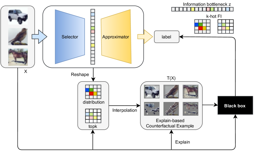
Figure 1: Overall flowchart of XCR. On the one hand, the selector and approximator structure extract $k$-hot feature importance explanations. On the other hand, XCR retains the black-box model by combining the feature importance interpretation of $k$-hot with the original input.

3.2 Black-Box Model Retrain

As shown in Fig. 1, We propose an explanation-based retraining pipeline. Specifically, as discussed in Sec. 3.1, existing L2X methods[7, 2] describe the behavior of black-box models by approximating them. However, this explanation process may have little to do with the black-box model’s internal structure but much to do with the structure and parameters of the L2X model. We strongly believe that this is similar to the situation described in [16] and is also a social misalignment in explanation. The human expectation is that feature importance explanations can reflect how models learn to use feature explanations as evidence for a particular decision. However, the presence of OOD affects FI explanations with model hyperparameters, random seeds of initialization, and data ordering[32, 11, 48]. In L2X, the approximator also uses the FI explanation data to approximate the black-box model, so naturally, there is a social misalignment. In addition, approximating black-box models can also introduce social misalignment. Specifically, the social expectation during the training process is to explain the black-box model. However, the L2X method does not pay attention to details of the black-box model but only to the input and output of the black-box model.
Therefore, we propose to use the original labels to generate feature importance explanations without approximating the black-box model, and then use the generated feature importance explanations as counterfactual input to join the black-box model for retraining.

4 Experiment and Results

We carry out experiments on popular vision datasets. We describe evaluation metrics of XAI, robustness, and OOD calibration in Sec. 4.1. We state the unnecessary use of imitating the behavior of the black-box model in L2X in Sec. 4.2. We explain the explanation-based counterfactual training process of the black-box model in detail and evaluate the XCR method in Sec. 4.3.

4.1 Objective Evaluation Metrics

We evaluate the XCR method in both the explanation and OOD calibration to compare it with existing methods.

4.1.1 XAI Evaluation Metrics

As far as we know, there is no generally accepted evaluation system for the XAI model. Therefore, in order to ensure the credibility of the results, we selected the evaluation indicators used in [16, 49, 5] for comparison. The explanation $e$ is described in [16] as a $k$-sparse binary vector in ${\{0,1\}}^{d}$, where $d$ is the dimensionality of the feature space. The explanation $e$ is similar to the $k$-hot vector encoding the information bottleneck in Sec. 3.2. However, in image classification tasks, $k$-hot vectors need to be reshaped and upsampled to fit the image size. For models $f$ and information bottleneck $z$ where the model output is the class classification probability, $\mathbf{Sufficiency}$ can be defined as:

$$\mathbf{Suff}(f,\mathbf{x},\mathbf{z},s)=f(x)_{\hat{y}}-f(\rm T_{s}(\mathbf{x},\mathbf{z}))_{\hat{y}}$$ (7)

where $\hat{y}=\arg\max_{y}f(x)_{y}$ is the predicted class, $T_{s}(\mathbf{x},\mathbf{z})$ is feature importance explanations extracted from information bottlenecks, $s$ is the proportion of information retained.

We also follow the Average Drop and Average Increase in [5]. The Average Drop is expressed as $\sum_{i=1}^{N}\frac{\max(0,Y_{i}^{c}-E_{i}^{c})}{Y_{i}^{c}}$. The Average Increase is expressed as $\sum_{i=1}^{N}\frac{Sign(Y_{i}^{c}<E_{i}^{c})}{N}$. Where $Y_{i}^{c}$ is the predicated probability for class $c$ on image $i$ and $E_{i}^{c}$ is the predicated probability for class $c$ with k-hot explanation map region image. $Sign$ will return $1$ if input is $True$. The Fidelity is the consistency of the FI-explained sample and the output of the original sample input into the model.

4.1.2 Model Performance and OOD Calibration Metrics

The performance of the original approximator can be used as a reference but is not decisive because the black-box model needs to be retrained later. The structure of the original selector and approximator may be simple, and the extracted vital feature information is only a tiny proportion. Thus, there will be performance loss like most XAI methods. We mainly use the image classification accuracy of the retrained model on the (corrupted-)vision dataset to evaluate model performance.
To evaluate the robustness and OOD calibration performance of the model after the XCR method is used, we use the benchmark proposed in [20]. Negative Log-Likelihood (NLL[17]), Expected Calibration Error (ECE[30]) and Brier[4] are also used to compare with the existing methods [45].

Table 1: Explanation metrics across methods, parameters, and datasets. We compare feature extraction with different retain ratios and different datasets (CIFAR10/100) when $patchsize=2$. Moreover, we report the evaluation metrics at each $\beta$ value. Accuracy and explanation metrics Average Drop and Average Increase are used to compare VIBI with our method.

Dataset	k	$\beta$	Accuracy $\uparrow$		Avg Drop $\downarrow$		Ave Inc $\uparrow$
			VIBI	XCR	VIBI	XCR	VIBI	XCR
CIFAR10	16	0.1	0.649	0.550	0.717	0.359	0.050	0.117
	16	0.01	0.675	0.618	0.825	0.362	0.039	0.092
	16	0.001	0.686	0.648	0.851	0.533	0.042	0.061
	32	0.1	0.737	0.765	0.192	0.119	0.166	0.219
	32	0.01	0.334	0.791	0.065	0.539	0.341	0.057
	32	0.001	0.758	0.751	0.670	0.143	0.045	0.182
	64	0.1	0.786	0.828	0.090	0.015	0.287	0.450
	64	0.01	0.785	0.856	0.232	0.249	0.166	0.154
	64	0.001	0.796	0.847	0.200	0.208	0.183	0.159
CIFAR100	32	0.01	0.418	0.449	0.455	0.193	0.086	0.191
	32	0.001	0.449	0.483	0.510	0.642	0.061	0.032
	64	0.01	0.496	0.567	0.099	0.104	0.261	0.265
	64	0.001	0.496	0.574	0.417	0.169	0.101	0.199

4.2 Learning to Explain without Imitation

Based on the VIBI method described in [2], we change the imitation behavior of the approximator to fitting the original labels, thereby ignoring the influence of the black-box model. We use ResNet28-10 trained according to [56] as the black-box model output for the L2X approximation. In the explained structure, ResNet18 is used as a selector, and ResNets[18] of various structures are used as approximators to adapt to different hyperparameter requirements. We use the CIFAR10/100 datasets and search for parameters $patchsize=\{2,4\}$, $k=\{8,16,32,64\}$ and $\beta=\{1,0.1,0.01,0.001\}$, part of the experimental results of CIFAR10/100 are shown in Table 1. More intuitively, we show the image’s explanation in Fig. 2. Please refer to Supplementary Materials S2 and S3 for more detailed results.
From the explanation results for different parameters and datasets, there is no significant difference between VIBI and our XCR method. With $k=16$ and a low feature retaining rate of $6.25\%$, VIBI’s approximator has slightly better accuracy than our XCR method, but VIBI’s XAI metric performs poorly. At regular feature retention rates of $12.5\%$ and $25\%$, our XCR method outperforms the original VIBI method on most metrics. Fig. 2 also visually shows that our XCR can generate meaningful results under the same parameter settings, and there is no significant difference from imitating the black-box model. Even the XCR explanations of some images make more sense than VIBI intuitively.

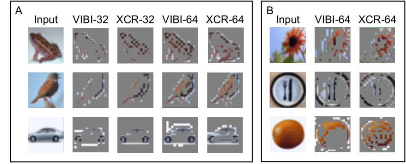
Figure 2: VIBI based on imitating the black-box model and our feature extraction without imitation. A. CIFAR10 dataset, we select the top-$32$ and top-$64$ explanation patches to show. B. CIFAR100 dataset, we select the top-$64$ explanation patches to show.

4.3 Counterfactual Retraining

As discussed in Sec. 4.2, the original label can be used directly without imitating the black-box model. We use the standard-trained ResNet28-10 as the black-box model without using additional data in [56], which is convenient to compare the results in [45]. In order to simplify the experiment, we use the same simple selectors and approximators as Sec. 4.2 with not too many parameters. We do not rule out the possibility of using more complex selectors and approximators to get better results. We use the CIFAR10/100 datasets and the benchmark proposed in [20], with the corruption image datasets CIFAR10-C, CIFAR100-C with 16 types of noises with 5 severity scales. The robustness and performance improvement of OOD calibration brought by the XCR method is verified.

4.3.1 Parameter Search in Retraining

When retraining, we set the learning rate to 0.1 according to the training process set in [56], the depth of the Wide-ResNet is set to $28$, the widen factor is set to $10$, and dropout is not used. The vanilla model was trained for 200 epochs as a comparison. Similar to Sec. 4.2, we do not modify the vanilla model and use a consistent model structure and the same training process, but only add counterfactual samples. Through pre-experiments, we find that XCR performs best when the patch size is 2. We perform a grid search on the XCR parameters, including $k={16,32,64}$ and $\beta={0.1,0.01,0.001}$. The results compared with existing methods are shown in Table 2, and the specific results of parameter grid search are shown in Supplementary Material S2. Our XCR method when $k=32$,$\beta=0.001$ beats all methods in accuracy on corrupted data, and also outperforms most existing methods such as single-pass method DUQ[47], SNGP[28] and even multi-pass method Deep Ensembles[26], MC Dropout[15], GSD[45] in NLL, ECE.

Table 2: Calibration metrics across methods and datasets. The experimental results are averaged with 10 random seeds. $\dagger$ represents the result in [45]. Our method when $k=32$, $\beta=0.001$ beats all methods in accuracy on corrupted data, and also outperforms most existing methods in NLL, ECE.

Dataset	Method	Accuracy $\uparrow$		ECE $\downarrow$		NLL $\downarrow$
		Clean	Corrupt	Clean	Corrupt	Clean	Corrupt
CIFAR10	Vanilla$\dagger$	96.0	72.9	0.023	0.153	0.158	1.059
	DUQ$\dagger$	94.7	71.6	0.034	0.183	0.239	1.348
	SNGP$\dagger$	95.9	74.6	0.018	0.090	0.138	0.935
	Deep Ensembles$\dagger$	96.6	77.9	0.010	0.087	0.114	0.815
	MC Dropout$\dagger$	96.0	70.0	0.021	0.116	0.173	1.152
	GSD$\dagger$	96.6	77.9	0.007	0.069	0.108	0.773
	Ours XCR	96.3	80.6	0.002	0.062	0.122	0.711
CIFAR100	Vanilla$\dagger$	79.8	50.5	0.085	0.239	0.872	2.756
	DUQ$\dagger$	78.5	50.4	0.119	0.281	0.980	2.841
	SNGP$\dagger$	79.9	49.0	0.025	0.117	0.847	2.626
	Deep Ensembles$\dagger$	80.2	54.1	0.021	0.138	0.666	2.281
	MC Dropout$\dagger$	79.6	42.6	0.050	0.202	0.825	2.881
	GSD$\dagger$	83.0	54.1	0.018	0.086	0.614	2.042
	Ours XCR	85.0	56.5	0.002	0.095	0.530	2.113

The training process when $k=32$, $\beta=0.001$ is shown in Fig. 3. We plot the metrics of the training set and the validation set explained by $\mathbf{Topk}$ and $\mathbf{Softmax}$ during the training process and compare them with vanilla results. It can be seen from the training process of 200 rounds that when we use the distribution explanation mode, that is, when $\mathbf{Softmax}$ is selected as the map function of processing the information bottleneck, the convergence of the model is better than $\mathbf{Topk}$. Our XCR method improves the robustness of the black-box model without significantly different from vanilla convergence speed. The validation loss of the XCR method on a dataset with a small number of categories is slightly higher than that of the vanilla method. However, the effect is not apparent, and the validation loss on a dataset with many categories is lower than that of the vanilla method.

4.3.2 Model Performance without Temperature Calibration

In the existing calibration methods, the temperature parameters of the DNNs head need to be calibrated on the validation set, such as [45]. Access to the validation set is limited to many problems, so we hope to achieve satisfactory calibration results without using the validation set calibration. We perform Our experiments on GSD[45] and XCR methods without validation set calibration, then the OOD calibration metrics and model accuracy are compared. The results are shown in Table 3. We reproduce the experimental results using the same parameter settings of the GSD[45] open source code and add experiments without calibration on the validation set. We find that the uncalibrated GSD method performs worse than our XCR method. Our XCR method, even without validation set calibration, exhibits satisfactory image classification accuracy on the corrupted dataset. When evaluating without validation set temperature calibration, ECE, NLL and Brier metrics are not significantly different between GSD and our XCR method.

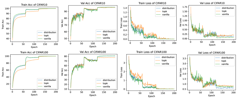
Figure 3: Convergence curves and accuracy curves when $k=32$, $\beta=0.001$.

Table 3: Calibration metrics when validation set is not used. The experimental results are averaged with 10 random seeds. Our method when $k=32$, $\beta=0.001$ exhibits satisfactory image classification accuracy on the corrupted dataset. ECE, NLL and Brier metrics are not significantly different between GSD and our XCR method.

		CIFAR10				CIFAR100
		Acc $\uparrow$	ECE $\downarrow$	NLL $\downarrow$	Brier$\downarrow$	Acc $\uparrow$	ECE $\downarrow$	NLL $\downarrow$	Brier$\downarrow$
Clean	GSD	96.28	0.013	0.147	0.006	79.74	0.018	0.815	0.003
	XCR	96.61	0.015	0.153	0.006	80.98	0.034	0.773	0.003
Corrupted	GSD	69.33	0.091	0.838	0.035	48.75	0.118	2.315	0.007
	XCR	80.25	0.104	0.841	0.031	58.20	0.120	2.148	0.006

4.3.3 Explanation Performance after Retraining

Before retraining, as shown by the evaluation metrics in Table 1, the explanation performance of the model is not good. After applying our XCR method, the model’s explanation fidelity, Average Drop, Average Increase, and Sufficiency are all significantly improved to a satisfactory level. The results can be found in Table 4. For more details, please refer to Supplementary Material S2.

Table 4: Explanation metrics when XCR is used. To illustrate that XCR can maintain high explainability while calibrating the model, we evaluate the retrained model using Fidelity, Average Drop, Average Increase, and Sufficiency and find that it is significantly better than that in Sec. 4.2 result.

Dataset	k	Fidelity $\uparrow$	Avg Drop $\downarrow$	Avg Inc $\uparrow$	Suff $\downarrow$
CIFAR10	16	0.984	0.016	0.497	0.008
	32	0.972	0.029	0.491	0.018
	64	0.985	0.015	0.438	0.008
CIFAR100	32	0.880	0.108	0.549	0.020
	64	0.887	0.100	0.534	0.021

4.3.4 Compare with Random Result

[21] shows that many methods are inferior to random mask results, so we generate random $k$-hot importance vectors to add to retraining and compare with XCR results. The results are shown in Supplementary Material S2, indicating that the FI-based XCR method outperforms the random mask method both on $\mathbf{Topk}$ and $\mathbf{Softmax}$ method.

5 Conclusion

In this paper, we argue that the imitation of the black-box model can be omitted in existing post-hoc L2X exploration methods that only care about the input and output of the model. We then propose an eXplanation-based Counterfactual Retraining (XCR) method to calibrate the OOD problem in XAI. XCR can be used to improve the model’s robustness and OOD calibration ability. Because the validation set is inaccessible in most cases, we also show that XCR outperforms existing methods without using the validation set for calibration. After retraining, the XAI evaluation metrics of the black-box model will enhance significantly.

References

- [1] Anders, C.J., Neumann, D., Samek, W., Müller, K.R., Lapuschkin, S.: Software for dataset-wide xai: From local explanations to global insights with zennit, corelay, and virelay. arXiv preprint arXiv:2106.13200 (2021)
- [2] Bang, S., Xie, P., Lee, H., Wu, W., Xing, E.: Explaining a black-box by using a deep variational information bottleneck approach. In: Proc. of AAAI (2021)
- [3] Bau, D., Zhu, J.Y., Strobelt, H., Zhou, B., Tenenbaum, J.B., Freeman, W.T., Torralba, A.: Gan dissection: Visualizing and understanding generative adversarial networks. In: Proc. of ICLR (2018)
- [4] Brier, G.W., et al.: Verification of forecasts expressed in terms of probability. Monthly weather review (1950)
- [5] Chattopadhay, A., Sarkar, A., Howlader, P., Balasubramanian, V.N.: Grad-cam++: Generalized gradient-based visual explanations for deep convolutional networks. In: Proc. of WACV (2018)
- [6] Chefer, H., Gur, S., Wolf, L.: Transformer interpretability beyond attention visualization. In: Proc. of CVPR (2021)
- [7] Chen, J., Song, L., Wainwright, M., Jordan, M.: Learning to explain: An information-theoretic perspective on model interpretation. In: Proc. of ICML (2018)
- [8] Cui, X., Wang, D., Wang, Z.J.: Chip: Channel-wise disentangled interpretation of deep convolutional neural networks. IEEE Transactions on Neural Networks and Learning Systems (2019)
- [9] Dai, Z., Liu, H., Le, Q., Tan, M.: Coatnet: Marrying convolution and attention for all data sizes. Proc. of NeurIPS (2021)
- [10] Deng, H., Ren, Q., Chen, X., Zhang, H., Ren, J., Zhang, Q.: Discovering and explaining the representation bottleneck of dnns. arXiv preprint arXiv:2111.06236 (2021)
- [11] Dodge, J., Ilharco, G., Schwartz, R., Farhadi, A., Hajishirzi, H., Smith, N.: Fine-tuning pretrained language models: Weight initializations, data orders, and early stopping. arXiv preprint arXiv:2002.06305 (2020)
- [12] Dosovitskiy, A., Beyer, L., Kolesnikov, A., Weissenborn, D., Zhai, X., Unterthiner, T., Dehghani, M., Minderer, M., Heigold, G., Gelly, S., et al.: An image is worth 16x16 words: Transformers for image recognition at scale. arXiv preprint arXiv:2010.11929 (2020)
- [13] Fong, R., Patrick, M., Vedaldi, A.: Understanding deep networks via extremal perturbations and smooth masks. In: Proc. of ICCV (2019)
- [14] Foret, P., Kleiner, A., Mobahi, H., Neyshabur, B.: Sharpness-aware minimization for efficiently improving generalization. arXiv preprint arXiv:2010.01412 (2020)
- [15] Gal, Y., Ghahramani, Z.: Dropout as a bayesian approximation: Representing model uncertainty in deep learning. In: Proc. of ICML (2016)
- [16] Hase, P., Xie, H., Bansal, M.: The out-of-distribution problem in explainability and search methods for feature importance explanations. Proc. of NeurIPS (2021)
- [17] Hastie, T., Tibshirani, R., Friedman, J.H., Friedman, J.H.: The elements of statistical learning: data mining, inference, and prediction. Springer (2009)
- [18] He, K., Zhang, X., Ren, S., Sun, J.: Identity mappings in deep residual networks. In: Proc. of ECCV (2016)
- [19] Hedström, A., Weber, L., Bareeva, D., Motzkus, F., Samek, W., Lapuschkin, S., Höhne, M.M.C.: Quantus: An explainable ai toolkit for responsible evaluation of neural network explanations. arXiv preprint arXiv:2202.06861 (2022)
- [20] Hendrycks, D., Dietterich, T.: Benchmarking neural network robustness to common corruptions and perturbations. In: Proc. of ICLR (2018)
- [21] Hooker, S., Erhan, D., Kindermans, P.J., Kim, B.: A benchmark for interpretability methods in deep neural networks. Proc. of NeurIPS (2019)
- [22] Jacovi, A., Goldberg, Y.: Aligning faithful interpretations with their social attribution. Transactions of the Association for Computational Linguistics (2021)
- [23] Jain, S., Wallace, B.C.: Attention is not explanation. In: Proc. of AACL (2019)
- [24] Jang, E., Gu, S., Poole, B.: Categorical reparameterization with gumbel-softmax. arXiv preprint arXiv:1611.01144 (2016)
- [25] Kolesnikov, A., Beyer, L., Zhai, X., Puigcerver, J., Yung, J., Gelly, S., Houlsby, N.: Big transfer (bit): General visual representation learning. In: Proc. of ECCV (2020)
- [26] Lakshminarayanan, B., Pritzel, A., Blundell, C.: Simple and scalable predictive uncertainty estimation using deep ensembles. Proc. of NeurIPS (2017)
- [27] Li, X.H., Cao, C.C., Shi, Y., Bai, W., Gao, H., Qiu, L., Wang, C., Gao, Y., Zhang, S., Xue, X., et al.: A survey of data-driven and knowledge-aware explainable ai. IEEE Transactions on Knowledge and Data Engineering (2020)
- [28] Liu, J., Lin, Z., Padhy, S., Tran, D., Bedrax Weiss, T., Lakshminarayanan, B.: Simple and principled uncertainty estimation with deterministic deep learning via distance awareness. Proc. of NeurIPS (2020)
- [29] Lundberg, S.M., Lee, S.I.: A unified approach to interpreting model predictions. Proc. of NeurIPS (2017)
- [30] Naeini, M.P., Cooper, G., Hauskrecht, M.: Obtaining well calibrated probabilities using bayesian binning. In: Proc. of AAAI (2015)
- [31] Petsiuk, V., Das, A., Saenko, K.: Rise: Randomized input sampling for explanation of black-box models. arXiv preprint arXiv:1806.07421 (2018)
- [32] Probst, P., Boulesteix, A.L., Bischl, B.: Tunability: importance of hyperparameters of machine learning algorithms. The Journal of Machine Learning Research (2019)
- [33] Qiu, L., Yang, Y., Cao, C.C., Liu, J., Zheng, Y., Ngai, H.H.T., Hsiao, J., Chen, L.: Resisting out-of-distribution data problem in perturbation of xai. arXiv preprint arXiv:2107.14000 (2021)
- [34] Ren, J., Li, M., Liu, Z., Zhang, Q.: Interpreting and disentangling feature components of various complexity from dnns. In: Proc. of ICML (2021)
- [35] Ren, J., Zhang, D., Wang, Y., Chen, L., Zhou, Z., Chen, Y., Cheng, X., Wang, X., Zhou, M., Shi, J., et al.: A unified game-theoretic interpretation of adversarial robustness. arXiv preprint arXiv:2111.03536 (2021)
- [36] Ribeiro, M.T., Singh, S., Guestrin, C.: "why should i trust you?" explaining the predictions of any classifier. In: Proc. of KDD (2016)
- [37] Selvaraju, R.R., Cogswell, M., Das, A., Vedantam, R., Parikh, D., Batra, D.: Grad-cam: Visual explanations from deep networks via gradient-based localization. In: Proc. of ICCV (2017)
- [38] Shen, W., Ren, Q., Liu, D., Zhang, Q.: Interpreting representation quality of dnns for 3d point cloud processing. Proc. of NeurIPS (2021)
- [39] Shen, Y., Yang, C., Tang, X., Zhou, B.: Interfacegan: Interpreting the disentangled face representation learned by gans. IEEE transactions on pattern analysis and machine intelligence (2020)
- [40] Shrikumar, A., Greenside, P., Kundaje, A.: Learning important features through propagating activation differences. In: Proc. of ICML (2017)
- [41] Shwartz-Ziv, R., Tishby, N.: Opening the black box of deep neural networks via information. arXiv preprint arXiv:1703.00810 (2017)
- [42] Simonyan, K., Vedaldi, A., Zisserman, A.: Deep inside convolutional networks: Visualising image classification models and saliency maps. In: Proc. of ICLR (2014)
- [43] Smilkov, D., Thorat, N., Kim, B., Viégas, F., Wattenberg, M.: Smoothgrad: removing noise by adding noise. arXiv preprint arXiv:1706.03825 (2017)
- [44] Sundararajan, M., Taly, A., Yan, Q.: Axiomatic attribution for deep networks. In: Proc. of ICML (2017)
- [45] Tian, J., Yung, D., Hsu, Y.C., Kira, Z.: A geometric perspective towards neural calibration via sensitivity decomposition. Proc. of NeurIPS (2021)
- [46] Tishby, N., Pereira, F.C., Bialek, W.: The information bottleneck method. arXiv preprint physics/0004057 (2000)
- [47] Van Amersfoort, J., Smith, L., Teh, Y.W., Gal, Y.: Uncertainty estimation using a single deep deterministic neural network. In: Proc. of ICML (2020)
- [48] Van Rijn, J.N., Hutter, F.: An empirical study of hyperparameter importance across datasets. In: Proc. of KDD (2017)
- [49] Wang, H., Wang, Z., Du, M., Yang, F., Zhang, Z., Ding, S., Mardziel, P., Hu, X.: Score-cam: Score-weighted visual explanations for convolutional neural networks. In: Proc. of CVPR (2020)
- [50] Wiegreffe, S., Pinter, Y.: Attention is not not explanation. In: Proc. of EMNLP (2019)
- [51] Wortsman, M., Ilharco, G., Gadre, S.Y., Roelofs, R., Gontijo-Lopes, R., Morcos, A.S., Namkoong, H., Farhadi, A., Carmon, Y., Kornblith, S., et al.: Model soups: averaging weights of multiple fine-tuned models improves accuracy without increasing inference time. arXiv preprint arXiv:2203.05482 (2022)
- [52] Xie, C., Tan, M., Gong, B., Wang, J., Yuille, A.L., Le, Q.V.: Adversarial examples improve image recognition. In: Proc. of CVPR (2020)
- [53] Xu, A., Raginsky, M.: Information-theoretic analysis of generalization capability of learning algorithms. Proc. of NeurIPS (2017)
- [54] Xu, Z.J.: Understanding training and generalization in deep learning by fourier analysis. arXiv preprint arXiv:1808.04295 (2018)
- [55] Yang, Z., Liu, Y., Bao, C., Shi, Z.: Interpolation between residual and non-residual networks. In: Proc. of ICML (2020)
- [56] Zagoruyko, S., Komodakis, N.: Wide residual networks. In: Proc. of BMVC (2016)
- [57] Zeiler, M.D., Fergus, R.: Visualizing and understanding convolutional networks. In: Proc. of ECCV (2014)