Model-Free Feedback Constrained Optimization Via Projected Primal-Dual Zeroth-Order Dynamics

Abstract

In this paper, we propose a model-free feedback solution method to solve generic constrained optimization problems, without knowing the specific formulations of the objective and constraint functions. This solution method is termed projected primal-dual zeroth-order dynamics (P-PDZD) and is developed based on projected primal-dual gradient dynamics and extremum seeking control. In particular, the P-PDZD method can be interpreted as a model-free controller that autonomously drives an unknown system to the solution of the optimization problem using only output feedback. The P-PDZD can properly handle both the hard and asymptotic constraints, and we develop the decentralized version of P-PDZD when applied to multi-agent systems. Moreover, we prove that the P-PDZD achieves semi-global practical asymptotic stability and structural robustness. We then apply the decentralized P-PDZD to the optimal voltage control problem in power distribution systems with square probing signals, and the simulation results verified the optimality, robustness, and adaptivity of the P-PDZD method.

I Introduction

This paper studies the real-time feedback control design that aims at autonomously steering a physical system to the solution of a constrained optimization problem. It relates to the emerging paradigm called feedback optimization [1, 2] that interconnects optimization iterations in closed-loop with the optimal control of physical plants. This type of control design has recently attracted considerable attention and can be applied in a wide range of fields [3], such as electric power grids [4, 5, 6], communication networks [7, 8], transportation systems [9], etc. However, designing such controllers for real physical systems is particularly challenging because of two major obstacles. One is the lack of accurate system models, as many real systems, such as power grids, are too complex to model and are subject to unknown time-varying disturbances. The other obstacle is the need to properly handle various constraints, including physical laws, control saturation, artificial performance requirements, etc., which significantly complicate the problem. This paper aims to develop model-free feedback solution methods for solving general constrained optimization, so that the solution methods can be interpreted as the desired feedback controllers that overcome these two obstacles.

To address the lack of system models or tackle intrinsically hard-to-model problems, model-free control and optimization schemes have been widely studied. Instead of pre-establishing a static model from first principles or historical data, model-free approaches probe the unknown system and online learn its characteristics from real-time measurements or other feedback. Reinforcement learning (RL) [10, 11] is a prominent type of model-free technique that is concerned with how agents take sequential actions in an uncertain interactive environment and learn from the feedback to maximize the cumulative reward. Despite its huge success in games, applying RL to the control of physical plants is still under development and entails many limitations [12], such as safety and scalability issues, limited theoretical guarantee, etc. Moreover, RL focuses on the cumulative performance over Markov decision processes [13], which is beyond our scope of feedback control design that steers a system to an optimal steady state.

An alternative type of model-free technique is extremum seeking (ES) control [14, 15], which is a classic adaptive control method and has regained research momentum due to its theoretical advances [16, 17]. The basic idea of ES is to perturb the system with a probing signal and estimate the gradient of the objective function solely based on the output feedback, and then it drives the system to an extremum state via a gradient descent flow-like structure. In this way, ES exhibits a close connection with zeroth-order optimization (ZO) approaches [18], which optimize using only function evaluations, and ES can be regarded as the continuous-time version of single-point ZO [19]. Due to its model-free feedback nature, ES has been applied to the control of various black-box or hard-to-model systems, such as voltage control in power systems [4], combustion control of thermal engines [20], photovoltaic maximum power point tracking [21], etc. Hence, ES is particularly suitable for the model-free feedback control problem that this paper studies.

Despite the theoretical advances and practical applications, one of the major limitation of existing ES schemes is that the constraints are not well enforced. For real-world physical systems, their constraints are of different natures and can be categorized into two types: hard constraints and asymptotic constraints [2]. Hard constraints refer to the physical control saturation or actuator capacity limits that should be satisfied all the time, such as the generation capacity of a power plant. Asymptotic constraints refer to soft physical limits or artificial performance requirements that can be violated temporarily during transient processes but should be met in the long-term steady state, e.g., the thermal limits of power lines and voltage limits imposed by industrial standards [22], the comfortable temperature ranges required in building climate control, etc. Properly handling these two types of constraints is essential to ensure the stability and optimality of the closed-loop system. However, most existing ES methods are confined to unconstrained problems, or use barrier or penalty functions to incorporate constraints into the objective [23, 24, 25, 26], which may not guarantee precise constraints enforcement. Besides, saddle point dynamics [27, 28, 29], projection [30, 31], and submanifolds [32] have been adopted to account for the constraints in ES. But these schemes generally do not distinguish between hard and asymptotic constraints, or only consider one type of constraints in their problems.

In this paper, we propose a new real-time zeroth-order feedback solution method, named projected primal-dual zeroth-order dynamics (P-PDZD), for solving generic constrained optimization problems with both hard and asymptotic constraints. In particular, the proposed P-PDZD method can be interpreted as a model-free feedback controller that steers a physical system to the solution of the constrained optimization problem, without the need to know the specific formulations of the objective and constraint functions. By exploiting real-time system feedback, the P-PDZD method is inherently robust and adaptive to time-varying unknown disturbances. The P-PDZD method is developed based on projected primal-dual gradient dynamics (P-PDGD) and ES control (continuous-time ZO). The contributions and merits of the proposed P-PDZD method are summarized below.

• (Model-Free). The P-PDZD only needs the zeroth-order information, i.e., function evaluations, of the objective and constraint functions, while their mathematical formulations and gradient information are not required.

• (Constraints and Optimality). By using projection, the P-PDZD guarantees that the hard constraints are always satisfied. By convergence, the asymptotic constraints are respected and optimality is achieved when the P-PDZD reaches the steady states.

• (Multi-Agent). The P-PDZD naturally extends to the cooperative multi-agent problems, and can be implemented in a decentralized fashion, where each agent performs computations only in the space of its individual decision variable and can preserve its own private information.

• (Performance Guarantee). By using averaging theory and singular perturbation theory, we prove that the P-PDZD achieves semi-global practical asymptotic stability and structure robustness. Moreover, we demonstrate the optimality, robustness, and adaptivity of the P-PDZD via extensive numerical experiments.

This paper generalizes our previous work [4] that is dedicated to the optimal voltage control problem in power systems. Compared to [4], this paper considers a generic constrained optimization problem, adopts general probing signals rather than only sinusoidal waves, and provides the complete theoretical proof techniques and insights, etc.

The remainder of this paper is organized as follows: Section II introduces the problem formulation and application examples. Section III develops the P-PDZD method and presents its multi-agent version. Section IV analyzes the theoretical performance of P-PDZD. Numerical experiments are conducted in Section V, and conclusions are drawn in Section VI.

Notations. We use unbolded lower-case letters for scalars, and bolded lower-case letters for column vectors. $\mathbb{R}_{+}:=[0,+\infty)$ denotes the set of non-negative real values. $\mathbb{B}$ denotes a closed unit ball of appropriate dimension. $||\cdot||$ denotes the L2-norm of a vector. $[\bm{x};\bm{y}]:=[\bm{x}^{\top},\bm{y}^{\top}]^{\top}$ denotes the column merge of vectors $\bm{x},\bm{y}$. Define the index set $[n]:=\{1,\cdots,n\}$ for a positive integer $n$. Denote the distance between a point $\bm{x}\in\mathbb{R}^{n}$ and a nonempty closed set $\mathcal{X}\subseteq\mathbb{R}^{n}$ as $||\bm{x}||_{\mathcal{X}}:=\underset{\bm{\bm{y}}\in\mathcal{X}}{\inf}\,||\bm{y}-\bm{x}||.$ Define the (point) projection that projects a point $\bm{x}\in\mathbb{R}^{n}$ onto the set $\mathcal{X}$ as $\mathrm{Proj}_{\mathcal{X}}(\bm{x}):=\underset{\bm{y}\in\mathcal{X}}{\mathrm{arg\,inf}}\,||\bm{y}-\bm{x}||.$

II Problem Formulation and Application Examples

In this section, we first introduce the problem formulation and the settings of available information. Then, we present several application examples to justify the problem settings.

II-A Problem Formulation

Consider solving the constrained optimization problem:

Obj. $$\min_{\bm{x}}\,f(\bm{x})$$ (1a)

s.t. $$\ \bm{x}\in\mathcal{X}$$ (1b)

$$\ g_{j}(\bm{x})\leq 0,\qquad j\in[m],$$ (1c)

where $\bm{x}\in\mathbb{R}^{n}$ is the decision variable and $f:\mathbb{R}^{n}\to\mathbb{R}$ is the objective function. $\mathcal{X}\subseteq\mathbb{R}^{n}$ denotes the feasible set of $\bm{x}$. The function vector $\bm{g}:=[g_{1};g_{2};\cdots;g_{m}]:\mathbb{R}^{n}\to\mathbb{R}^{m}$ describes the inequality constraints. In particular, we consider that only zero-order information is available for functions $f$ and $\bm{g}$, which is formally stated in the following assumption.

Assumption 1.

(Available Information). The mathematical formulations of functions $f$ and $g_{1},\cdots,g_{m}$ as well as their derivatives of any order are unavailable, while one can only access the function evaluations of functions $f$ and $g_{1},\cdots,g_{m}$. Besides, the feasible set $\mathcal{X}$ is known.

Remark 1.

The motivation and rationale of the above problem setting are explained below.

• The above problem is motivated by the feedback control design that aims at steering an unknown plant in real time to an optimal solution of problem (1). We simplify the plant dynamics model by the static input-to-output mapping functions $f(\bm{x})$ and $\bm{g}(\bm{x})$, as we consider fast stable plant dynamics that converge immediately given any input $\bm{x}\in\mathcal{X}$ and we aim to optimize the steady-state performance. It is referred to as the timescale separation property with fast plant dynamics and slow control, which is commonly assumed in ES control [17, 14].

• For many complex systems, their system models, captured by the static maps $f(\bm{x})$ and $\bm{g}(\bm{x})$, may be unavailable or too costly to estimate in practice. Fortunately, the widespread deployment of smart meters and sensors provides real-time measurements of the system outputs. These measurements can be interpreted as the function evaluations of $f$ and $\bm{g}$ and used as system feedback to circumvent the unknown model information.

• In the problem (1), we distinguish hard constraints and asymptotic constraints by the feasible set $\mathcal{X}$ (1b) and the inequalities (1c), respectively. Thus, the feasible set $\mathcal{X}$ (1b) should always be satisfied, while the inequalities (1c) can be violated temporarily during transient processes but need to be satisfied in the steady states.

II-B Application Examples

Below we present three application examples to illustrate the problem setting, including optimal voltage control, building thermal control, and TCP flow control.

II-B1 Optimal Voltage Control

Consider an electric distribution grid with the monitored node set $\mathcal{M}$ and the controllable device set $\mathcal{C}$. Each node $j\in\mathcal{M}$ has real-time measurement on the nodal voltage magnitude $v_{j}$, and the power injection $\bm{x}_{i}$ of each device $i\in\mathcal{C}$ can be controlled to maintain the voltage profiles $(v_{j})_{j\in\mathcal{M}}$ within an acceptable interval $[\underline{v}_{j},\bar{v}_{j}]$. Then, the optimal voltage control [33, 34] is to achieve the optimal power injection $\bm{x}\coloneqq(\bm{x}_{i})_{i\in\mathcal{C}}$ that solves the problem (2):

Obj. $$\min_{\bm{x}}\,\sum_{i\in\mathcal{C}}c_{i}(\bm{x}_{i})$$ (2a)

s.t. $$\ \bm{x}_{i}\in\mathcal{X}_{i}, i\,\in\,\mathcal{C}$$ (2b)

$$\ \underline{v}_{j}\leq v_{j}(\bm{x})\leq\bar{v}_{j}, j\in\mathcal{M}.$$ (2c)

Here, $c_{i}(\cdot)$ is the cost function and $\mathcal{X}_{i}$ is the power capacity feasible set. A key challenge is that the voltage function $v_{j}(\bm{x})$ is generally unknown and hard to estimate, because it actually captures the entire power grid information, including network topology, power line parameters, power flow equations, uncontrollable power disturbances, etc. To address this issue, the real-time voltage measurement $v_{j}$ can be leveraged as system feedback to circumvent the unknown models [33, 34].

II-B2 Building Thermal Control

Consider a building that is divided into $n$ thermal zones [35]. For each zone $i\in[n]$, there is an air conditioner (AC) unit operating at the power of $p_{i}$ with the rated power capacity $\bar{p_{i}}$. Let $T_{i}$ be the temperature of $i$-th zone and $[\underline{T},\bar{T}]$ be the comfortable temperature interval. Then, the building thermal control [36, 37, 38] is to optimize the AC power profile to solve the optimization problem (3):

Obj. $$\min_{(p_{i})_{i\in[n]}}\ \,\sum_{i=1}^{n}p_{i}$$ (3a)

s.t. $$\,p_{i}\in[\,0,\,\bar{p}_{i}\,], \qquad i\in[n]$$ (3b)

$$\underline{T}\leq T_{i}\big{(}(p_{j})_{j\in\mathcal{S}_{i}}\big{)}\leq\bar{T},\quad \qquad i\in[n].$$ (3c)

Here, $\mathcal{S}_{i}\subseteq[n]$ denotes the set of zones whose AC operations affect the temperature of $i$-th zone via heat transfer. The function $T_{i}(\cdot)$ describes the input-to-output map from AC power to the temperature of $i$-th zone, which is complex and usually unknown in practice, as it is affected by many factors, such as the heat capacity, ambient temperature, human flow, solar irradiance, etc. Nevertheless, smart thermometers can be deployed to measure the zone temperature $T_{i}$ in real time.

II-B3 TCP Flow Control

Consider a communication network with the link set $\mathcal{L}$ and the data source set $\mathcal{S}$. Denote $r_{s}$ as the transmission rate of source $s\in\mathcal{S}$ with the lower limit $\underline{r}_{s}$ and upper limit $\bar{r}_{s}$. The data from a source $s$ flows through a prescribed path consisting of links $\mathcal{L}_{s}\subseteq\mathcal{L}$ to its destination. The TCP flow control problem [8, 39] aims to achieve the optimal transmission rates that solve the problem (4):

Obj. $$\max_{(r_{s})_{s\in\mathcal{S}}}\ \,\sum_{s\in\mathcal{S}}U_{s}(r_{s})$$ (4a)

s.t. $$\,r_{s}\in[\underline{r}_{s},\bar{r}_{s}], \quad s\in\mathcal{S}$$ (4b)

$$g_{l}\big{(}(r_{s})_{s\in\mathcal{S}_{l}}\big{)}\geq 0,\qquad \quad\,l\in\mathcal{L},$$ (4c)

where $U_{s}:\mathbb{R}\to\mathbb{R}$ is the utility function for source $s\in\mathcal{S}$, and $\mathcal{S}_{l}\coloneqq\{s\,|l\in\mathcal{L}_{s}\}$ denotes the set of sources that contain the link $l\in\mathcal{L}$ in their paths. Equation (4c) describes the transmission capacity constraint of each link $l\in\mathcal{L}$, and function $g_{l}(\cdot)$ denotes the map from the transmission rates $(r_{s})_{s\in\mathcal{S}_{l}}$ to the spare capacity of link $l$. In practice, an accurate formulation of function $g_{l}(\cdot)$ may be unavailable due to exogenous disturbances, noises and fatigue, especially for wireless communication. The utility function $U_{s}(\cdot)$ may also be too complex to model. Instead, one can observe the realization of the utility $U_{s}$ and monitor the spare transmission capacity $g_{l}$ of each link in real time.

We note that the presented application problems (3)-(2) are simplified models for illustrative purposes; see the cited references therein for more details. Other applications, such as resource allocation [40], optimal network flow [41], etc., can also fit into the problem setting described in Section II-A.

III Model-Free Feedback Algorithm Design and Application to Multi-Agent Systems

In this section, we first solve problem (1) with the projected primal-dual gradient dynamics (P-PDGD) method. Then, we integrate ES control into P-PDGD and develop the projected primal-dual zeroth-order dynamics (P-PDZD) method, which is the model-free feedback solution algorithm for solving (1). Lastly, we propose the decentralized application of P-PDZD for cooperative multi-agent systems.

We make the following two standard assumptions on problem (1) to render it a convex optimization with strong duality.

Assumption 2.

The feasible set $\mathcal{X}$ is nonempty, closed, and convex. The functions $f$ and $g_{1},\cdots,g_{m}$ are convex and have locally Lipschitz gradients on $\mathcal{X}$.

Assumption 3.

The problem (1) has a finite optimum, and the Slater’s conditions hold for (1).

These assumptions above are mainly for theoretical analysis, and the proposed methods are practically applicable to a wider range of problems that may not satisfy these assumptions. This will be validated by the numerical experiments in Section V.

III-A Projected Primal-Dual Gradient Dynamics

To solve the problem (1), we introduce the dual variable $\bm{\lambda}:=(\lambda_{j})_{j\in[m]}\in\mathbb{R}_{+}^{m}$ for the inequality constraints (1c) and formulate the saddle point problem (5):

$$\max_{\bm{\lambda}\in\mathbb{R}_{+}^{m}}\,\min_{\bm{x}\in\mathcal{X}}\,L(\bm{x},\bm{\lambda}):=f(\bm{x})+\sum_{j=1}^{m}\lambda_{j}g_{j}(\bm{x}),$$ (5)

where $L(\bm{x},\bm{\lambda})$ is the Lagrangian function. By strong duality (Assumption 2 and 3), the $\bm{x}$-component of any saddle point of (5) is an optimal solution to problem (1). Denote $\bm{z}:=[\bm{x};\bm{\lambda}]$ and define $\mathcal{Z}:=\mathcal{X}\times\mathbb{R}_{+}^{m}$ as the feasible set of $\bm{z}$ in (5).

To ensure the satisfaction of the hard feasible set, we adopt the P-PDGD (6) to solve the saddle point problem (5):

$$\dot{\bm{x}} =k_{x}\Big{[}\mathrm{Proj}_{\mathcal{X}}\Big{(}\bm{x}-\alpha_{x}\big{(}\nabla f(\bm{x})+\!\sum_{j=1}^{m}\lambda_{j}\nabla g_{j}(\bm{x})\big{)}\Big{)}\!-\bm{x}\Big{]}$$ (6a)

$$\dot{\lambda}_{j} =k_{\lambda}\Big{[}\mathrm{Proj}_{\mathbb{R}_{+}}\Big{(}\lambda_{j}+\alpha_{\lambda}\,g_{j}(\bm{x})\Big{)}-\lambda_{j}\Big{]},\quad j\in[m],$$ (6b)

where $k_{x},k_{\lambda},\alpha_{x},\alpha_{\lambda}$ are positive parameters.

The P-PDGD (6) is referred to as a globally projected (or continuous projected) dynamical system [42, 43]. As the projection operator $\mathrm{Proj}_{\mathcal{Z}}(\cdot)$ is globally Lipschitz with the Lipschitz constant $L=1$ [44, Proposition 2.4.1], one can show that the vector field of (6) is locally Lipschitz on $\mathcal{Z}$ under Assumption 2. This is different from the widely-used discontinuous projected dynamics [45, 46, 47] that project the gradient flow onto the tangent cone of the feasible set, and thus they need sophisticated analysis tools for discontinuous dynamical systems. The use of continuous projection facilitates the performance analysis of the P-PDGD (6) and the subsequent P-PDZD method (12). Nevertheless, the discontinuous version of P-PDGD, i.e., (18), can also be used to develop model-free feedback solution algorithms; see Appendix A for details.

By [42, Lemma 3], the solution $\bm{z}(t)$ of the P-PDGD (6) will stay within $\mathcal{Z}$ for all time $t\geq t_{0}$ when the initial condition $\bm{z}(t_{0})\in\mathcal{Z}$. Hence, the hard feasible set (1b) can be always satisfied during the solution process. Moreover, the following proposition states the equivalence between the optimal solutions of the saddle point problem (5) and the equilibrium points of P-PDGD (6). And Theorem 1 states the global asymptotic convergence of P-PDGD (6).

Proposition 1.

Under Assumption 2 and 3, any equilibrium point of the P-PDGD (6) is an optimal solution of the saddle point problem (5), vice versa.

Theorem 1.

(Global Asymptotic Stability of P-PDGD). Under Assumption 2 and 3, the P-PDGD (6) with initial condition $\bm{z}(t_{0})\in\mathcal{Z}$ has a unique continuously differentiable solution $\bm{z}(t):[t_{0},+\infty)\to\mathcal{Z}$, and the solution $\bm{z}(t)$ globally asymptotically converges to an optimal solution $\bm{z}^{*}$ of the saddle point problem (5).

The proof of Proposition 1 is provided in Appendix B-A. The proof of Theorem 1 mainly follows the asymptotic stability of globally projected dynamical systems [42] [48, Lemma 2.4]; see Appendix B-B for a detailed proof.

However, the P-PDGD (6) method is not implementable under the information setting in Section II-A, because it needs the gradient information of functions $f$ and $\bm{g}$ in (6a). This issue is addressed in the next subsection using ES control.

III-B Projected Primal-Dual Zeroth-Order Dynamics

To address the issue of unknown gradients, we integrate ES control into the P-PDGD (6) and develop the projected primal-dual zeroth-order dynamics (P-PDZD) to solve problem (1) using only zeroth-order feedback. Specifically, we add a small periodic probing signal $\epsilon_{a}d(\omega_{i}t)$ to each element $x_{i}$ of the decision variable $\bm{x}$, leading to

$$\hat{x}_{i}(t)=x_{i}(t)+\epsilon_{a}d(\omega_{i}t),\quad i\in[n],$$ (7)

where positive parameters $\epsilon_{a}$ and $\omega_{i}$ denote the amplitude and frequency, respectively. We make the following standard assumption on the probing signal $d(t)$ [49].

Assumption 4.

The probing signal $d(t)$ is a periodic function with the period $T=2\pi$ that satisfies

$$\int_{0}^{T}\!\!d(t)dt=0;\ \frac{1}{T}\int_{0}^{T}\!\!d^{2}(t)dt=\eta_{d}\!>0;\ \max_{t\in[0,T]}\!d(t)=1.$$ (8)

Common choices of the probing signals $d(t)$ include sinusoidal wave $d_{\sin}(t)\coloneqq\sin(t)$, square wave $d_{\mathrm{sq}}(t)$ defined as (9), triangular wave, etc. [49]

$$d_{\mathrm{sq}}(t)\coloneqq\begin{cases}1,&t\in[2k\pi,(2k\!+\!1)\pi]\\ -1,&t\in[(2k\!+\!1)\pi,2(k\!+\!1)\pi]\end{cases},\ k\in\mathbb{Z}.$$ (9)

In addition, the frequency parameters $\bm{\omega}:=(\omega_{i})_{i\in[n]}\in\mathbb{R}^{n}$ are defined as

$$\qquad\omega_{i}=\frac{2\pi}{\epsilon_{\omega}}\kappa_{i},\quad i\in[n],$$ (10)

where $\epsilon_{\omega}$ is a small positive parameter and $\kappa_{i}\neq\kappa_{j}$ for all $i\neq j$ are positive rational numbers. Thus each decision variable $x_{i}$ is assigned with a different frequency $\omega_{i}$ to be distinguished for all $i\in[n]$. Moreover, the frequency parameters should satisfy the orthogonality condition (11):

$$\int_{0}^{T_{ij}}\!\!d(\omega_{i}t)d(\omega_{j}t)\,dt=0,\quad\forall i\neq j,$$ (11)

where $T_{ij}$ is the period of $d(\omega_{i}t)d(\omega_{j}t)$. The sinusoidal signal $d_{\mathrm{sin}}(t)$ naturally satisfies the condition (11). When the square signal $d_{\mathrm{sq}}(t)$ is used, we also require $\kappa_{i}\neq(2k+1)\kappa_{j}$ for all $k\in\mathbb{Z}$ and $i\neq j$ to meet the condition (11).

Denote $\bm{d}(\bm{\omega}t)\coloneqq(d(\omega_{i}t))_{i\in[n]}$ as the column vector that collects all probing signals. Then based on the P-PDGD (6), we develop the P-PDZD (12) to solve the saddle point point (5), which only needs the zeroth-order information (i.e., function evaluations) of $f,\bm{g}$.

$$\dot{\bm{x}} =k_{x}\Big{[}\mathrm{Proj}_{\hat{\mathcal{X}}\ }\big{(}\bm{x}-\alpha_{x}\,\bm{\xi}\big{)}-\bm{x}\Big{]}$$ (12a)

$$\dot{\bm{\lambda}} =k_{\lambda}\Big{[}\mathrm{Proj}_{\mathbb{R}_{+}^{m}\!}\big{(}\bm{\lambda}+\alpha_{\lambda}\bm{\mu}\big{)}-\bm{\lambda}\Big{]}$$ (12b)

$$\begin{split}\dot{\bm{\xi}}&=\!\frac{1}{\epsilon_{g}}\Big{[}\!-\bm{\xi}\!+\!\frac{1}{\epsilon_{a}\eta_{d}}\Big{(}f(\hat{\bm{x}}(t))\!+\!\bm{\lambda}^{\top}\bm{g}(\hat{\bm{x}}(t))\Big{)}\bm{d}(\bm{\omega}t)\Big{]}\end{split}$$ (12c)

$$\dot{\bm{\mu}} =\!\frac{1}{\epsilon_{g}}\Big{[}\!-\bm{\mu}+\bm{g}(\hat{\bm{x}}(t))\Big{]}.$$ (12d)

In (12c), $\eta_{d}$ is a constant defined in (8), which depends on the type of the probing signal. For example, $\eta_{d}=\frac{1}{2}$ when the sinusoidal signal $d_{\mathrm{sin}}$ is used, and $\eta_{d}=1$ for the square signal $d_{\mathrm{sq}}$. $\epsilon_{g}$ is a small positive parameter. $\hat{\bm{x}}(t):=(\hat{x}_{i}(t))_{i\in[n]}=\bm{x}(t)+\epsilon_{a}\bm{d}(\bm{\omega}t)$ denotes the perturbed decision values at time $t$. In (12a), $\hat{\mathcal{X}}\subseteq\mathcal{X}$ is the largest closed convex shrunken feasible set such that $\bm{x}+\epsilon_{a}\mathbb{B}\subseteq\mathcal{X}$ for any $\bm{x}\in\hat{\mathcal{X}}$, and $\hat{\mathcal{X}}\to\mathcal{X}$ as $\epsilon_{a}\to 0$. Note that $\hat{\bm{x}}(t)$ is the actual implemented action or input to the system for evaluation, while $\bm{x}(t)$ is an intermediate computational variable. Thus we replace $\mathcal{X}$ by $\hat{\mathcal{X}}$ in (12a) to ensure $\hat{\bm{x}}(t)\in\mathcal{X}$ all the time.

The major difference between the P-PDGD (6) and the P-PDZD (12) is the introduction of new variables $\bm{\xi}:=(\xi_{i})_{i\in[n]}\in\mathbb{R}^{n}$ and $\bm{\mu}:=(\mu_{j})_{j\in[m]}\in\mathbb{R}^{m}$ together with their fast dynamics (12c) (12d). The rationale and benefit of this design are explained in Remark 2.

Remark 2.

Intuitively, the introduced variables $\bm{\xi}$ and $\bm{\mu}$ can be regarded as the real-time approximation of $\nabla_{\bm{x}}L$ and $\bm{g}$, respectively. With a sufficiently small $\epsilon_{g}$, the P-PDZD (12) exhibit a time-scale separation between the slow dynamics (12a) (12b) and the fast dynamics (12c) (12d). As a result, $\xi_{i}$ and $\mu_{j}$ quickly converge to the second terms in the right-hand sides of (12c) and (12d), and the second terms are indeed the approximation of $\nabla_{\bm{x}}L(\bm{x},\bm{\lambda})$ and $\bm{g}(\bm{x})$, respectively. The advantages by introducing these fast dynamics are twofold:

• It facilitates theoretical analysis of the projected dynamics via averaging theory, as the high-frequency time-varying terms associated with $\bm{d}(\bm{\omega}t)$ are moved out of the projection operator. Besides, the fast dynamics are linear and thus can be easily handled by singular perturbation theory.

• The fast dynamics (12c) (12d) can be interpreted as low-pass filters for the estimation values, which can diminish the oscillations and improve the transient performance of the closed-loop system.

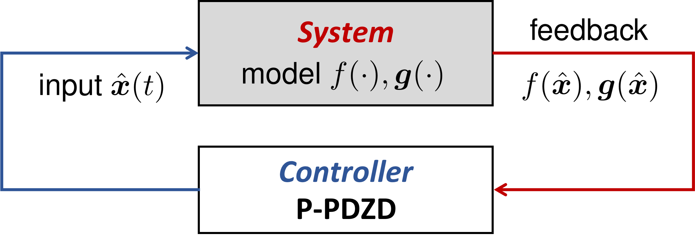
Figure 1: Implementation of the proposed P-PDZD method (12).

The P-PDZD (12) is the proposed optimal model-free feedback control scheme to steer the state of a black-box system to an optimal solution of problem (1). The implementation of the P-PDZD algorithm (12) is illustrated as Figure 1. At each time $t$, the controller feeds the input $\hat{\bm{x}}(t)$ to the black-box system and receives the corresponding zeroth-order feedback $f(\hat{\bm{x}}(t))$ and $\bm{g}(\hat{\bm{x}}(t))$, which are then used to update the input $\hat{\bm{x}}(t)$ according to the P-PDZD (12). Depending on the actual problem, the feedback can be the real-time measurements from a physical system, the simulation outputs from a complex simulator, or the observations from experiments.

Although developed based on the static optimization problem (1), the P-PDZD (12) can adapt to the dynamical system changes due to the use of real-time system feedback. The adaptivity and dynamic tracking performance of P-PDZD are demonstrated by the numerical simulations in Section V-D. Moreover, the P-PDZD (12) directly extends to the cooperative multi-agent problems and has a decentralized version, with each agent computing and executing its own actions. This will be elaborated in the next subsection. The theoretical analysis of the P-PDZD (12) is provided in Section IV. Besides, the same design idea can be applied to the discontinuous version of P-PDGD, which is presented in Appendix A.

III-C Decentralized P-PDZD for Multi-Agent Systems

Consider a multi-agent system with $N$ agents. Each agent $i\in[N]$ is associated with a local action $\bm{x}_{i}\in\mathbb{R}^{n_{i}}$, which is subject to the feasible set $\mathcal{X}_{i}\subseteq\mathbb{R}^{n_{i}}$, and $\sum_{i=1}^{N}n_{i}=n$. Let $\bm{x}\coloneqq(\bm{x}_{i})_{i\in[N]}\in\mathbb{R}^{n}$ be the joint action profile of all agents. The goal of the agents is to cooperatively find an optimal action profile $\bm{x}^{*}$ that solves the problem (13):

Obj. $$\min_{\bm{x}}\,\sum_{i=1}^{N}f_{i}(\bm{x}_{i})$$ (13a)

s.t. $$\,\bm{x}_{i}\in\mathcal{X}_{i}, \qquad i\in[N]$$ (13b)

$$\,g_{j}\big{(}(\bm{x}_{i})_{i\in\mathcal{S}_{j}}\big{)}\leq 0, \qquad j\in[m],$$ (13c)

where $\mathcal{S}_{j}\subseteq[N]$ denotes the set of agents that are involved in the $j$-th constraint described with function $g_{j}(\cdot)$. Define $\mathcal{J}_{i}\coloneqq\{j\,|i\in\mathcal{S}_{j}\}\subseteq[m]$ as the index set of constraints that involve the action $\bm{x}_{i}$ for each agent $i\in[N]$. The problem (13) is a multi-agent special case of the general form (1) and is motivated by the application examples presented in Section II-B. Similarly, we make the following assumption on the available information for the multi-agent system.

Assumption 5.

(Available Information for Multi-Agent System). The mathematical formulations of functions $f$ and $g_{1},\cdots,g_{m}$ as well as their derivatives of any order are unavailable. Each agent $i\in[N]$ can only access the function evaluations of $f_{i}$ and $(g_{j})_{j\in\mathcal{J}_{i}}$, and its own feasible set $\mathcal{X}_{i}$.

When the P-PDZD (12) is applied to solve problem (13), it directly becomes the decentralized P-PDZD (14). As illustrated in Figure 2, each agent $i\in[N]$ takes its own action $\hat{\bm{x}}_{i}(t)\coloneqq\bm{x}_{i}(t)+\epsilon_{a}\bm{d}(\bm{\omega}_{i}t)$ and receives the zeroth-order feedback $f_{i}(t)\coloneqq f_{i}(\hat{\bm{x}}_{i}(t))$ and $g_{j}(t)\coloneqq g_{j}\big{(}(\hat{\bm{x}}_{i}(t))_{i\in\mathcal{S}_{j}}\big{)}$ of all $j\in\mathcal{J}_{i}$. Then each agent $i$ updates its own action $\hat{\bm{x}}_{i}(t)$ according to (14):

$$\dot{\bm{x}}_{i} =k_{x}\Big{[}\mathrm{Proj}_{\hat{\mathcal{X}}_{i}}\big{(}\bm{x}_{i}-\alpha_{x}\bm{\xi}_{i}\big{)}-\bm{x}_{i}\Big{]}$$ (14a)

$$\dot{\lambda}_{j} =k_{\lambda}\Big{[}\mathrm{Proj}_{\mathbb{R}_{+}}\big{(}\lambda_{j}+\alpha_{\lambda}\,\mu_{j}\big{)}-\lambda_{j}\Big{]}, j\in\mathcal{J}_{i}$$ (14b)

$$\dot{\bm{\xi}}_{i} =\!\frac{1}{\epsilon_{g}}\Big{[}\!-\!\bm{\xi}_{i}+\!\frac{1}{\epsilon_{a}\eta_{d}}\big{(}f_{i}(t)\!+\!\sum_{j\in\mathcal{J}_{i}}\!\lambda_{j}g_{j}(t)\big{)}\bm{d}(\bm{\omega}_{i}t)\Big{]}$$ (14c)

$$\dot{\mu}_{j} =\frac{1}{\epsilon_{g}}\Big{[}-\!\mu_{j}+g_{j}(t)\Big{]}, j\in\mathcal{J}_{i}.$$ (14d)

In this way, the P-PDZD algorithm (14) is implemented in a decentralized manner, where each agent performs computations only in the space of its own decision variable and thus can preserve its private information. Moreover, the dynamics of $\lambda_{j}$ and $\mu_{j}$, i.e., (14b) and (14d), are indeed the same for all agents $i\in\mathcal{S}_{j}$. Hence, (14b) and (14d) only need to be executed once and then $\lambda_{j}$ is broadcast to the agents $i\in\mathcal{S}_{j}$ to update $\bm{x}_{i}$ and $\bm{\xi}_{i}$, which can avoid repeated computations.

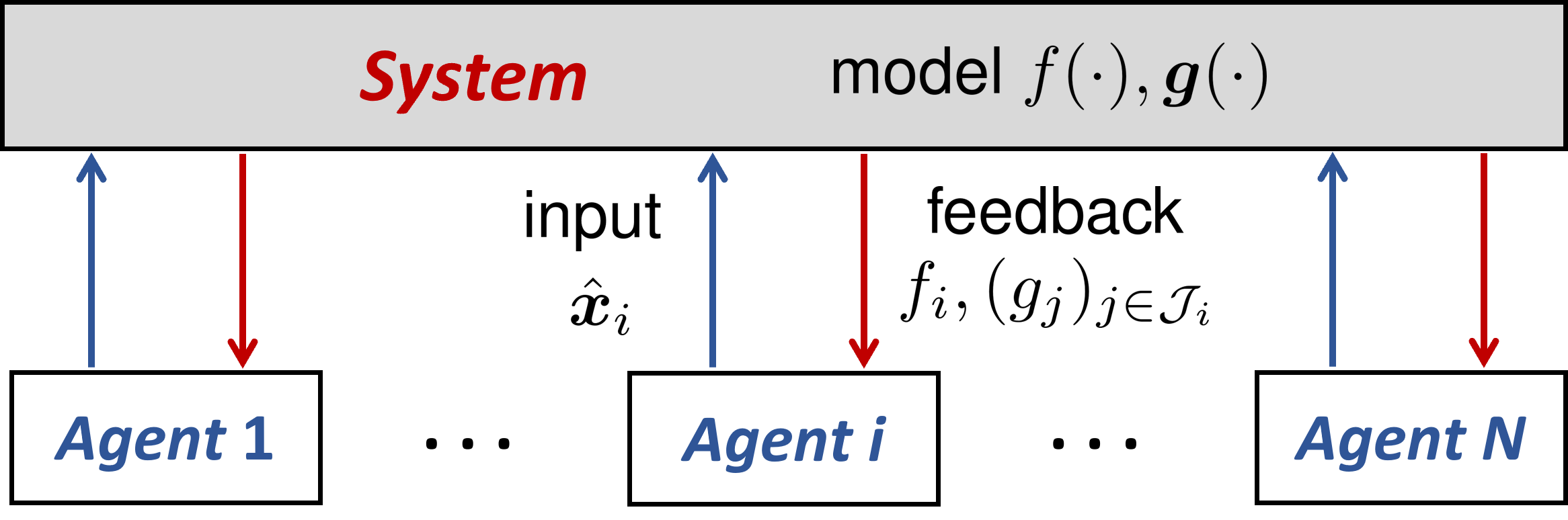
Figure 2: Implementation of decentralized P-PDZD (14) for multi-agent systems.

IV Performance Analysis of P-PDZD

In this section, we analyze the theoretical performance of the proposed P-PDZD method, including stability analysis and structural robustness to noises.

IV-A Stability Analysis

Denote $\bm{z}:=[\bm{x};\bm{\lambda}]$, $\bm{\psi}:=[\bm{\xi};\bm{\mu}]$, and $\hat{\mathcal{Z}}:=\hat{\mathcal{X}}\times\mathbb{R}^{m}_{+}$. Let $\hat{\mathcal{A}}$ be the saddle point set for the saddle point problem (5) with $\hat{\mathcal{X}}$. The stability properties of the P-PDZD (12) are stated as Theorem 2, which is proved based on averaging theory and singular perturbation theory. The detailed proof of Theorem 2 is provided in Appendix B-C.

Theorem 2.

(Semi-Global Practical Asymptotic Stability). Suppose that the saddle point set $\hat{\mathcal{A}}$ is compact. Under Assumptions 2, 3 and 4, there exists a class-$\mathcal{KL}$ function $\beta$ such that for any compact set $\mathcal{D}\subset\hat{Z}\times\mathbb{R}^{n+m}$ of initial condition $[\bm{z}(t_{0});\bm{\psi}(t_{0})]$, and any desired precision $\nu>0$, there exists $\epsilon_{g}^{*}>0$ such that for any $\epsilon_{g}\in(0,\epsilon_{g}^{*})$, there exists $\epsilon_{a}^{*}>0$ such that for any $\epsilon_{a}\in(0,\epsilon_{a}^{*})$, there exists $\epsilon_{\omega}^{*}>0$ such that for any $\epsilon_{\omega}\in(0,\epsilon_{\omega}^{*})$, the solution $\bm{z}(t)$ of the P-PDZD (12) satisfies

$$||\bm{z}(t)||_{\hat{\mathcal{A}}}\leq\beta(\,||\bm{z}(t_{0})||_{\hat{\mathcal{A}}},\,t-t_{0})+\nu,\ \ \forall t\geq t_{0}.$$ (15)

Theorem 2 indicates that, due to the small probing signal $\epsilon_{a}\bm{d}(\bm{\omega}t)$, the solution $\bm{z}(t)$ of the P-PDZD (12) will not converge to a fixed point anymore but rather to a small $\nu$-neighborhood of $\hat{\mathcal{A}}$. Nevertheless, by setting the parameters $(\epsilon_{g},\epsilon_{a},\epsilon_{\omega})$ sufficiently small, one can make this precision $\nu$ as small as desired.

The assumption of a compact saddle point set $\hat{\mathcal{A}}$ in Theorem 2 is standard for the use of averaging theory and singular perturbation theory. For many practical applications, the feasible set $\hat{\mathcal{X}}$ describes the physical capacity limits or control saturation and thus is naturally compact. In addition, we can replace the feasible region $\mathbb{R}_{+}^{m}$ of the dual variable $\bm{\lambda}$ by the feasible box set $[0,M_{\lambda}]^{m}$ with a sufficiently large $M_{\lambda}$. Thus the saddle point set $\hat{\mathcal{A}}\subseteq\hat{\mathcal{X}}\times[0,M_{\lambda}]^{m}$ is compact.

IV-B Structural Robustness

The P-PDZD method (12) heavily relies on function evaluations (or system feedback) to steer the decision to an optimal solution of problem (1). Then robustness is desirable to handle small disturbances and noises that are inevitable in practice. The following corollary of Theorem 2 [50] indicates that the P-PDZD (12) is structurally robust to small additive state noise.

Corollary 1.

(Structural Robustness). For any tuple of $(\epsilon_{g},\epsilon_{a},\epsilon_{\omega})$ that induces the bound (15), under the same conditions in Theorem 2, there exists $\bar{e}>0$ such that for any additive state noise $\bm{e}(t):[t_{0},+\infty)\!\to\!\mathbb{R}^{n}$ with $\sup_{t\geq t_{0}}||\bm{e}(t)||\leq\bar{e}$, the trajectory $\bm{z}(t)$ of the P-PDZD (12) with the additive state noise $\bm{e}(t)$ satisfies

$$||\bm{z}(t)||_{\hat{\mathcal{A}}}\leq\beta(||\bm{z}(t_{0})||_{\hat{\mathcal{A}}},\,t-t_{0})+2\nu,\ \ \forall t\geq t_{0}.$$ (16)

Comparing with (15), the P-PDZD (12) with small additive state noise $\bm{e}$ maintains similar convergence results, and the noise $\bm{e}$ leads to an additional precision $\nu$ term in (16).

V Numerical Experiments

In this section, we apply the proposed P-PDZD method to solve the optimal voltage control (OVC) problem described in Section II-B. We demonstrate the optimality, robustness, and adaptivity of the P-PDZD method via numerical experiments.

V-A Experiment Setup

We use the modified PG&E 69-node electric distribution network [51], shown as Figure 3, as the test system. Three photovoltaic (PV) power plants locate at nodes 35, 54 and 69, whose time-varying generations are treated as unknown system disturbances that jeopardize the voltage security. There are 7 static VAR compensators (SVCs) located at nodes 9, 20, 32, 43, 51, 57, 67, which are the controllable devices (depicted by the set $\mathcal{C}$) for voltage control under disturbances. The reactive power output of each SVC $i\in\mathcal{C}$ is the decision variable $x_{i}\in\mathcal{X}_{i}:=[-2,2.5]$ in the unit of MVar. We consider a known quadratic cost function $c_{i}(x_{i})=0.1x_{i}^{2}$ for all $i\in\mathcal{C}$. The monitored node set $\mathcal{M}$ includes nodes 3, 27, 35, 46, 54 and 69, which have real-time voltage measurements. The voltage of node 0 (slack node) is set as 1 p.u., and the lower and upper limits of voltage magnitude are set as $\underline{v}_{j}=0.95$ p.u. and $\bar{v}_{j}=1.05$ p.u. for all monitored nodes $j\in\mathcal{M}$. The unknown voltage function $\bm{v}(\bm{x}):=(v_{j}(\bm{x}))_{j\in\mathcal{M}}$ is simulated based on the full nonconvex Distflow model [52]. As a result, the OVC problem (2) does not satisfy Assumption 2 and is nonconvex. The power line impedances, nodal loads, and other parameters of the test system are provided in [53].

The OVC problem (2) fits into the multi-agent model (13), and thus the decentralized P-PDZD (14) can be applied to steer the SVC decisions $\bm{x}:=(x_{i})_{i\in\mathcal{C}}$ to an optimal solution of the OVC problem (2). See our previous work [4] for the detailed implementation of the decentralized P-PDZD. Unlike the sinusoidal probing signal used in [4], we use the square wave $d_{\mathrm{sq}}(t)$ (9) as the probing signal, because square waves are easier to implement in practice. For the P-PDZD algorithm, we set $\epsilon_{a}=\epsilon_{\omega}=\epsilon_{g}=0.025$, $\kappa_{i}=1.2+1.5i$ for $i=1,\cdots,7$, $\alpha_{x}=\alpha_{\lambda}=0.001$, and $k_{x}=50,k_{\lambda}=10$.

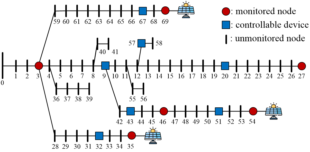
Figure 3: The modified PG&E 69-node electric distribution grid.

V-B Solving Static OVC Problem

Consider the test scenario when the three PV plants are suddenly shut down at time $t=0$ with zero power output, and voltage profiles tend to violate the lower limit due to the reduction of generation. With PV generations and loads being fixed, the OVC problem (2) is a static optimization. We then implement the decentralized P-PDZD (14) for real-time voltage regulation from the initial time $t=0$. The simulation results are shown as Figures 4, 5, and 6.

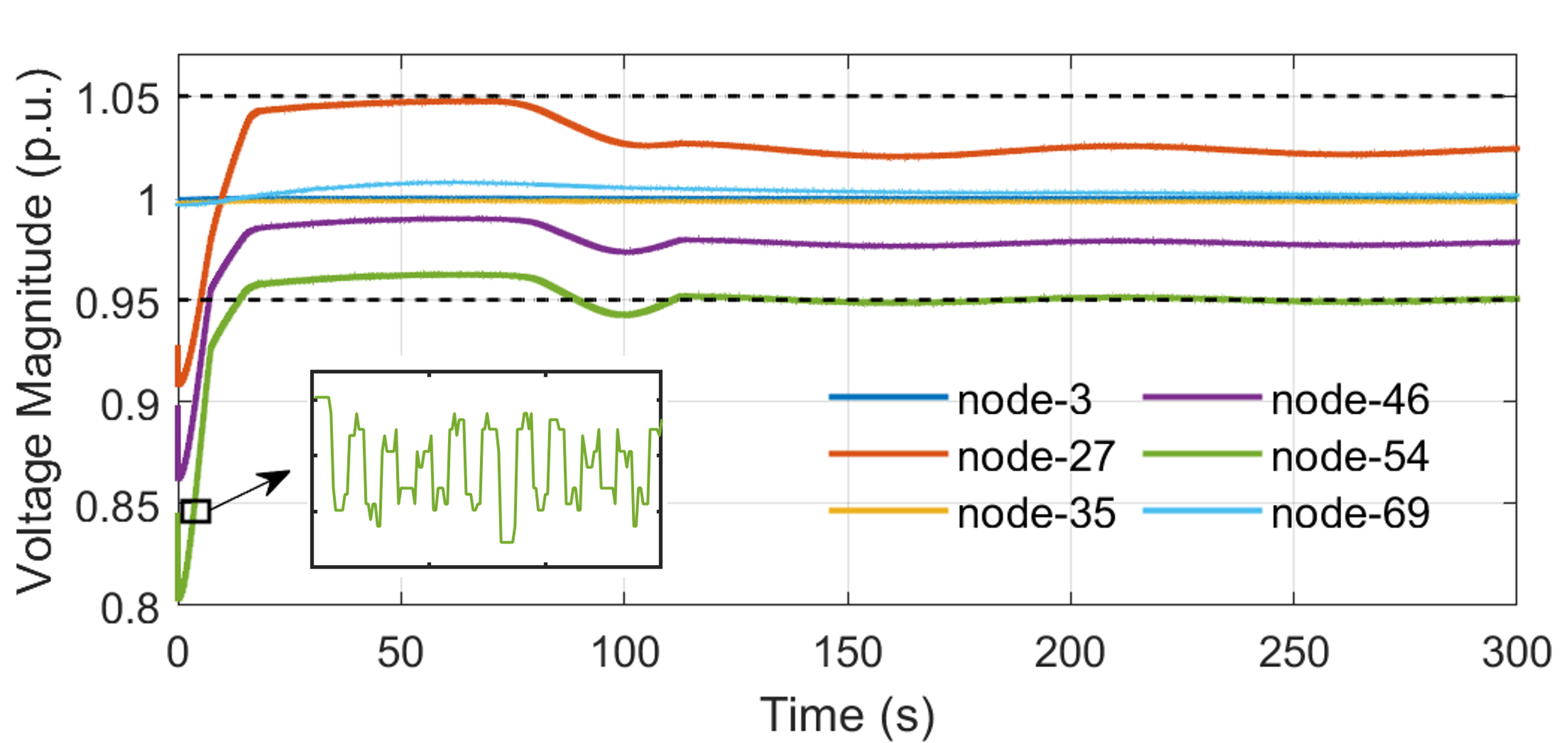
Figure 4: Voltage dynamics of the monitored nodes under static OVC problem (black dashed lines are the upper and lower voltage limits; the curve in the small box is the zoom-in view of voltage dynamics of node-54).

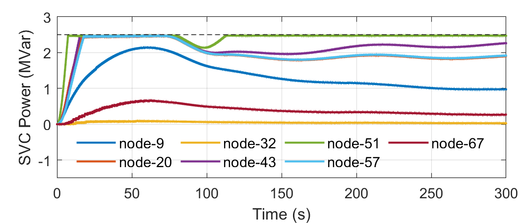
Figure 5: The implemented reactive power outputs $\hat{\bm{x}}(t)=\bm{x}(t)+\epsilon_{a}\bm{d}_{\mathrm{sq}}(\bm{\omega}t)$ of SVCs (the black dashed line denotes the upper power capacity limit).

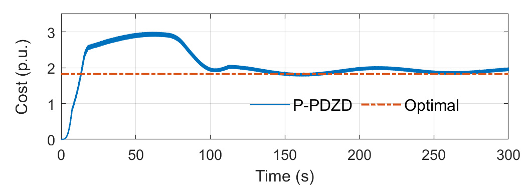
Figure 6: The dynamics of the total control cost, i.e., the objective (2a).

Figure 4 illustrates the voltage dynamics of all the monitored nodes. It is observed that the P-PDZD effectively brings the voltage profiles back to the acceptable interval $[0.95,1.05]$ (p.u.). When zooming in on the voltage dynamics, we can see the small-amplitude high-frequency oscillations, which are caused by the square probing signals. Figure 5 shows the dynamics of SVC reactive power outputs (i.e., decision variables). It is seen that the SVC powers quickly converge and always stay within the hard capacity limits due to the projection. The associated control cost is shown as Figure 6, where the cost of P-PDZD converges to the optimal value. It indicates that the P-PDZD method can steer the SVC decision to an optimal solution of the static OVC problem (2) solely based on real-time voltage measurement.

V-C Robustness to Measurement Noise

Measurement noises are inevitable in practice. This subsection considers the noisy voltage measurement $\tilde{v}^{\mathrm{mea}}_{j}(t)$, whose deviation from the base voltage value (1 p.u.) follows (17):

$$\tilde{v}^{\mathrm{mea}}_{j}(t)-1=(v_{j}(\bm{x}(t))-1)\times(1+\delta_{j}(t)),$$ (17)

where $v_{j}(\bm{x}(t))$ denotes the true voltage magnitude, and $\delta_{j}$ is the perturbation ratio. Assume that $\delta_{j}$ is a Gaussian random variable with $\delta_{j}\sim\mathcal{N}(0,\sigma^{2})$, which is independent across time $t$ and monitored nodes. We tune the standard deviation $\sigma$ from 0 to 0.5 to simulate different levels of noises and test the performance of the P-PDZD algorithm. Other settings are the same as those in Section V-B. The simulation results are shown as Figure 7, while the noiseless case with $\sigma=0$ is shown in Figure 4. From Figure 7, it is seen that the P-PDZD algorithm is robust to measurement noises and restores the voltage profiles to the acceptable interval in all the cases. Besides, higher levels of noises lead to larger oscillations in the voltage dynamics.

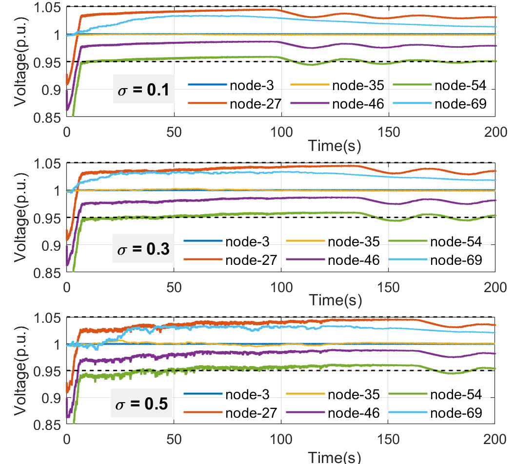
Figure 7: Voltage dynamics of the monitored nodes under different levels of measurement noises.

V-D Dynamic Tracking for Time-Varying OVC Problem

In practice, the power grid is a dynamic system with fluctuating loads and renewable generations. Hence, the unknown voltage function should be formulated as $\bm{v}(\bm{x};\bm{y}_{t})$, where $\bm{y}_{t}$ captures the time-varying components, and thus the OVC problem (2) is not static but is changing over time. In this experiment, we apply the time-varying PV generation, shown as Figure 8, to simulate the system changes, and continuously run the P-PDZD algorithm for real-time voltage control. The dynamics of the voltage profiles and control cost are shown as Figures 9 and 10, respectively. It is observed that the P-PDZD algorithm generally maintains the voltage profiles within the acceptable interval, although the voltage limits are violated very temporarily during the transient process. Moreover, the P-PDZD keeps tracking the optimal solution of the time-varying OVC problem. This verifies that by exploiting the real-time voltage measurement as system feedback, the P-PDZD can adapt to the dynamic system with time-varying disturbances and achieve self-optimizing performance.

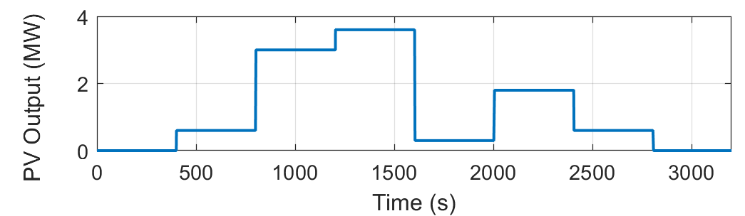
Figure 8: The time-varying total PV generation.

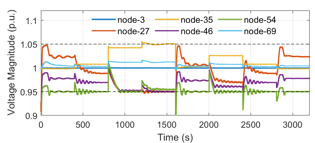
Figure 9: Voltage dynamics of the monitored buses under time-varying disturbances (black dashed lines are the upper and lower voltage limits).

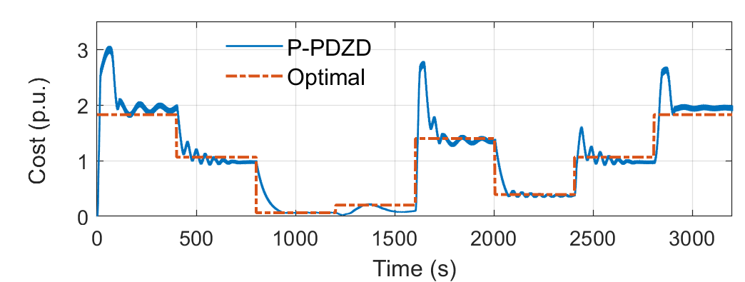
Figure 10: The control cost of P-PDZD and the optimal cost values over time.

VI Conclusion

In this paper, we propose the P-PDZD method to solve the generic constrained optimization problems with hard and asymptotic constraints in a model-free feedback manner. Using only zeroth-order feedback or output measurements, the proposed method can be interpreted as the model-free feedback controller that autonomously drive a black-box system to the solution of the optimization problem. We prove the semi-global practical asymptotic stability and robustness of the P-PDZD and present the decentralized version of P-PDZD when applied to multi-agent problems. The numerical experiments on the optimal voltage control problem with square probing signals demonstrate the optimality, robustness, and dynamic tracking capability of the P-PDZD method. For future work, we will incorporate the plant dynamics and study the discrete-time implementation of the P-PDZD.

Appendix A Model-Free Feedback Algorithm Design Using Discontinuous Projected Dynamics

The discontinuous projected primal-dual gradient dynamics (DP-PDGD) [45, 46, 47] to solve problem (5) is given by

$$\dot{\bm{x}} =k_{x}\cdot\mathrm{Proj}_{T_{\mathcal{X}}(\bm{x})}\big{(}-\!\nabla f(\bm{x})-\sum_{j=1}^{m}\lambda_{j}\nabla g_{j}(\bm{x})\big{)}$$ (18a)

$$\dot{\lambda}_{j} =k_{\lambda}\cdot\mathrm{Proj}_{T_{\mathbb{R}_{+}}(\lambda_{j})}\big{(}g_{j}(\bm{x})\big{)},\qquad j\in[m],$$ (18b)

where $k_{x},k_{\lambda}$ are positive parameters, and $T_{\mathcal{X}}(\bm{x})$ denotes the tangent cone to the set $\mathcal{X}$ at a point $\bm{x}\in\mathcal{X}$.

Denote $\bm{z}:=[\bm{x};\bm{\lambda}]$ and $\mathcal{Z}:=\mathcal{X}\times\mathbb{R}_{+}^{m}$. The DP-PDGD (18) projects the gradient flow of the Lagrangian function onto the tangent cone of the feasible set at the current point. When $\bm{z}(t)$ reaches the boundary of $\mathcal{Z}$, the projection operator restricts the gradient flow such that the solution $\bm{z}(t)$ of (18) remains in $\mathcal{Z}$. Hence, the DP-PDGD (18) is generally a discontinuous dynamical system [47]. It is also equivalent to reformulate the DP-PDGD (18) in the form of the vector projection (19) [55, Proposition 1]:

$$\dot{\bm{z}}=k_{z}\cdot\Pi_{\mathcal{Z}}(\bm{z},-\bm{h}(\bm{z})),\ \bm{h}(\bm{z}):=\begin{bmatrix}\nabla_{\bm{x}}L(\bm{x},\bm{\lambda})\\ -\nabla_{\bm{\lambda}}L(\bm{x},\bm{\lambda})\end{bmatrix},$$ (19)

where the vector projection of a direction vector $\bm{v}$ at a point $\bm{z}\in\mathcal{Z}$ with respect to $\mathcal{Z}$ is defined as

$$\Pi_{\mathcal{Z}}(\bm{z},\bm{v}):=\lim_{\delta\to 0^{+}}\frac{\mathrm{Proj}_{\mathcal{Z}}(\bm{z}+\delta\bm{v})-\bm{z}}{\delta}.$$ (20)

Since the vector field of (18) is discontinuous in general, the solution of the DP-PDGD (18) exists in the sense of an Caratheodory solution [56]. Under Assumption 2 and 3, one can show that the DP-PDGD (18) with initial condition $\bm{z}(t_{0})\in\mathcal{Z}$ globally asymptotically converges to an optimal solution $\bm{z}^{*}$ of the saddle point problem (5) [3, 47].

Then we apply the same design idea proposed in Section III-B to the DP-PDGD (18) and develop the discontinuous P-PDZD (DP-PDZD) (21) for solving (5).

$$\dot{\bm{x}} =k_{x}\cdot\mathrm{Proj}_{T_{\hat{\mathcal{X}}}(\bm{x})}\big{(}-\!\bm{\xi}\big{)}$$ (21a)

$$\dot{\bm{\lambda}} =k_{\lambda}\cdot\mathrm{Proj}_{T_{\mathbb{R}_{+}^{m}\!}(\bm{\lambda})}\big{(}\bm{\mu}\big{)}$$ (21b)

$$\text{Equations \eqref{eq:c:pdzd:psi} \eqref{eq:c:pdzd:mu}}.$$ (21c)

The DP-PDZD (21) is the same as the P-PDZD (12), except that the discontinuous projection approach is used in (21a) and (21b). It indicates that the DP-PDZD (21) has the same properties and merits as described in the introduction section. Besides, one can also prove the semi-global practical asymptotic stability of the DP-PDZD (21) by using our proof method in Appendix B-C, but it is more challenging because of the discontinuous dynamics, and the tools of differential inclusion and the notion of Krasovskii solutions [3, 56] can be used to complete the proof.

Appendix B Lemmas and Proofs

B-A Proof of Proposition 1

Proof. According to [57, Theorem 3.25], the KKT conditions of the saddle point problem (5) are given by

$$0\in\nabla f(\bm{x}^{*})+\sum_{j=1}^{m}\lambda_{j}^{*}\nabla g_{j}(\bm{x}^{*})+N_{\mathcal{X}}(\bm{x})$$ (22a)

$$\bm{x}^{*}\in\mathcal{X},\ g_{j}(\bm{x}^{*})\leq 0,\qquad\ \,\forall j\in[m]$$ (22b)

$$\lambda_{j}^{*}\geq 0,\,\lambda_{j}^{*}g_{j}(\bm{x}^{*})=0,\qquad\forall j\in[m].$$ (22c)

By definition, any equilibrium point $\bm{z}^{*}:=[\bm{x}^{*};\bm{\lambda}^{*}]$ of the P-PDGD (6) is equivalent to satisfy (23):

$$\bm{x}^{*} =\mathrm{Proj}_{\mathcal{X}}\Big{(}\bm{x}^{*}\!-\!\alpha_{x}\big{(}\nabla f(\bm{x}^{*})\!+\!\sum_{j=1}^{m}\lambda_{j}^{*}\nabla g_{j}(\bm{x}^{*})\big{)}\Big{)}$$ (23a)

$$\lambda_{j}^{*} =\mathrm{Proj}_{\mathbb{R}_{+}}\Big{(}\lambda_{j}^{*}+\alpha_{\lambda}\,g_{j}(\bm{x}^{*})\Big{)},\qquad\forall j\in[m],$$ (23b)

which is equivalent to (24):

$$-\!\nabla f(\bm{x}^{*})\!-\!\sum_{j=1}^{m}\lambda_{j}^{*}\nabla g_{j}(\bm{x}^{*})\in N_{\mathcal{X}}(\bm{x}),\ \bm{x}^{*}\in\mathcal{X}$$ (24a)

$$\lambda_{j}^{*}\geq 0,\ g_{j}(\bm{x}^{*})\leq 0,\ \lambda_{j}^{*}g_{j}(\bm{x}^{*})=0,\quad\forall j\in[m].$$ (24b)

By comparison, equations (22) and (24) are exactly the same. Thus Proposition 1 is proved.

B-B Proof of Theorem 1

We rewrite the P-PDGD (6) in a compact form as

$$\dot{\bm{z}}=\mathrm{Proj}_{\mathcal{Z}}(\bm{z}-\alpha\bm{h}(\bm{z}))-\bm{z}:=\bm{f}(\bm{z}),$$ (25)

where $\bm{h}(\bm{z})$ is defined in (19). Since $\mathrm{Proj}_{\mathcal{Z}}(\cdot)$ is a singleton and globally Lipschitz with constant $L=1$ [44, Proposition 2.4.1], the dynamics $\bm{f}(\bm{z})$ in (25) is locally Lipschitz on $\mathcal{Z}$ by Assumption 2, and thus there exists a unique continuously differentiable solution $\bm{z}(t)$ of (25) [56, Corollary 1]. Moreover, by [42, Lemma 3], we have that $\bm{z}(t)\in\mathcal{Z}$ for all time $t\geq t_{0}$ whenever $\bm{z}(t_{0})\in\mathcal{Z}$.

Denote $\bm{z}^{*}:=[\bm{x}^{*};\bm{\lambda}^{*}]$ as an optimal solution of (5). Then, consider the following Lyapunov function $V$:

$$V(\bm{z}) :=\frac{1}{2}||\bm{z}-\bm{z}^{*}||^{2}+L(\bm{x},\bm{\lambda}^{*})-L(\bm{x}^{*},\bm{\lambda})$$ (26)

$$\ =\frac{1}{2}||\bm{z}-\bm{z}^{*}||^{2}+L(\bm{x},\bm{\lambda}^{*})-L(\bm{x}^{*},\bm{\lambda}^{*})$$

$$\quad+L(\bm{x}^{*},\bm{\lambda}^{*})-L(\bm{x}^{*},\bm{\lambda})\geq\frac{1}{2}||\bm{z}-\bm{z}^{*}||^{2}.$$

The Lie derivative of $V$ along the P-PDGD (6) is

$$\mathcal{L}_{\bm{f}}V(\bm{z})=\nabla_{\bm{z}}V(\bm{z})^{\top}\bm{f}(\bm{z})=(\bm{z}-\bm{z}^{*}+\bm{h}(\bm{z}))^{\top}\bm{f}(\bm{z}).$$ (27)

One useful property is stated as Lemma 1.

Lemma 1.

For any $\alpha>0$, we have

$$(\bm{z}\!-\!\bm{z}^{*}+\alpha\bm{h}(\bm{z}))^{\top}\bm{f}(\bm{z})\leq\!-||\bm{f}(\bm{z})||^{2}\!-\alpha(\bm{z}\!-\!\bm{z}^{*})^{\top}\bm{h}(\bm{z}).$$

The proof of Lemma 1 follows [48, Lemma 2.4]. For completeness, we provide the proof as the three steps below:

1) We use the fact [45] that the projection operator satisfies

$$(\mathrm{Proj}_{\mathcal{Z}}(\bm{\gamma})-\bm{\beta})^{\top}(\bm{\gamma}-\mathrm{Proj}_{\mathcal{Z}}(\bm{\gamma}))\geq 0,$$ (28)

for all $\bm{\gamma}\in\mathbb{R}^{|\mathcal{Z}|},\bm{\beta}\in\mathcal{Z}$.

2) Let $\bm{\gamma}=\bm{z}-\alpha\bm{h}(\bm{z})$ and $\bm{\beta}=\bm{z}^{*}$, then (28) becomes

$$(\bm{f}({\bm{z}})+\bm{z}-\bm{z}^{*})^{\top}(\alpha\bm{h}(\bm{z})+\bm{f}({\bm{z}}))\leq 0.$$ (29)

3) Thus we obtain Lemma 1 by

$$\,(\bm{z}-\bm{z}^{*}+\alpha\bm{h}(\bm{z}))^{\top}\bm{f}({\bm{z}})$$

$$= \,(-\bm{f}({\bm{z}})+\bm{f}({\bm{z}})+\bm{z}-\bm{z}^{*}+\alpha\bm{h}(\bm{z}))^{\top}\bm{f}({\bm{z}})$$

$$= \,-\!||\bm{f}({\bm{z}})||^{2}+(\bm{f}({\bm{z}})+\bm{z}-\bm{z}^{*})^{\top}\bm{f}({\bm{z}})+\alpha\bm{h}(\bm{z})^{\top}\bm{f}({\bm{z}})$$

$$\leq \,-\!||\bm{f}({\bm{z}})||^{2}-\alpha(\bm{f}({\bm{z}})+\bm{z}-\bm{z}^{*})^{\top}\bm{h}(\bm{z})+\alpha\bm{h}(\bm{z})^{\top}\bm{f}({\bm{z}})$$

$$= \,-\!||\bm{f}({\bm{z}})||^{2}-\alpha(\bm{z}-{\bm{z}}^{*})^{\top}\bm{h}(\bm{z}),$$

where the inequality above is because of (29).

Using the result of Lemma 1 with $\alpha=1$, we obtain

$$\mathcal{L}_{\bm{f}}V(\bm{z})\leq-||\bm{f}({\bm{z}})||^{2}-(\bm{z}-\bm{z}^{*})^{\top}\bm{h}(\bm{z})$$

$$= \!-\!||\bm{f}({\bm{z}})||^{2}\!-\!(\bm{x}\!-\!\bm{x}^{*})^{\top}\nabla_{\bm{x}}L(\bm{x},\!\bm{\lambda})\!+\!(\bm{\lambda}\!-\!\bm{\lambda}^{*})^{\top}\nabla_{\bm{\lambda}}L(\bm{x},\!\bm{\lambda})$$

$$\leq \!-\!||\bm{f}({\bm{z}})||^{2}+\!L(\bm{x}^{*},\bm{\lambda})\!-\!L(\bm{x},\bm{\lambda})\!+\!L(\bm{x},\bm{\lambda})\!-\!L(\bm{x},\bm{\lambda}^{*})$$

$$= \!-\!||\bm{f}({\bm{z}})||^{2}+\!L(\bm{x}^{*}\!,\bm{\lambda})\!-\!L(\bm{x}^{*}\!,\bm{\lambda}^{*})\!+\!L(\bm{x}^{*}\!,\bm{\lambda}^{*})\!-\!L(\bm{x},\bm{\lambda}^{*})$$

$$\leq \!-\!||\bm{f}({\bm{z}})||^{2}\leq 0,$$ (30)

where the second inequality follows that $L(\bm{x},\bm{\lambda})$ is convex in $\bm{x}$ and concave in $\bm{\lambda}$.

Since $V(\bm{z})$ is radially unbounded and by (B-B), the trajectory $\bm{z}(t)$ of (25) remains bounded for all $t\geq t_{0}$. By LaSalle’s Theorem [58, Theorem 4.4], we have that $\bm{z}(t)$ converges to the largest invariant compact subset $\mathcal{M}$ contained in $\mathcal{S}$:

$$\mathcal{S}:=\big{\{}{\bm{z}}\in\mathcal{Z}:~{}\mathcal{L}_{\bm{f}}V(\bm{z})=0,\,V({\bm{z}})\leq V(\bm{z}(t_{0}))\big{\}}.$$ (31)

When $\mathcal{L}_{\bm{f}}V(\bm{z})=0$, we must have $L(\bm{x}^{*},\bm{\lambda})=L(\bm{x}^{*},\bm{\lambda}^{*})$ and $L(\bm{x},\bm{\lambda}^{*})=L(\bm{x}^{*},\bm{\lambda}^{*})$ by (B-B). Thus any point $\bm{z}\in\mathcal{M}$ is an optimal solution of the saddle point problem (5). Lastly, following the proof of [59, Theorem 15], one can show that $\bm{z}(t)$ eventually converges to a fixed optimal solution $\bm{z}^{*}$. Thus Theorem 1 is proved.

B-C Proof of Theorem 2

Denote $\bm{z}:=[\bm{x};\bm{\lambda}]$, $\bm{\psi}:=[\bm{\xi};\bm{\mu}]$, and $\bm{s}:=[\bm{z};\bm{\psi}]$. The P-PDZD (12) is reformulated in compact form as

$$\dot{\bm{s}}=\begin{bmatrix}\dot{\bm{z}}\\ \dot{\bm{\psi}}\end{bmatrix}=\begin{bmatrix}\bm{q}_{1}(\bm{z},\bm{\psi})\\ \frac{1}{\epsilon_{g}}(-\bm{\psi}+\bm{q}_{2}(t,\bm{z}))\end{bmatrix}:=\bm{q}(t,\bm{s}),$$ (32)

where function $\bm{q}_{1}(\bm{z},\bm{\psi})$ captures the dynamics (12a) (12b), and function $\bm{q}_{2}(t,\bm{z})$ is given by

$$\bm{q}_{2}:=\begin{bmatrix}\frac{1}{\epsilon_{a}\eta_{d}}\big{(}f(\hat{\bm{x}}(t))+\sum_{j=1}^{m}\lambda_{j}g_{j}(\hat{\bm{x}}(t))\big{)}\bm{d}(\bm{\omega}t)\\ \bm{g}(\hat{\bm{x}}(t))\end{bmatrix},$$ (33)

where the first part and the second part are associated with the dynamics (12c) of $\bm{\xi}$ and (12d) of $\bm{\mu}$, respectively.

We analyze the stability properties of system (32) using averaging theory and singular perturbation theory, which is divided into the following three steps.

Step 1) Construct a compact set to study the behavior of system (32) restricted to it.

To apply averaging theory and singular perturbation theory, it generally requires that the considered trajectories stay within predefined compact sets. Without loss of generality, we consider the compact set $[(\hat{\mathcal{A}}+\Delta\mathbb{B})\cap\hat{\mathcal{Z}}]\times\Delta\mathbb{B}$ for the initial condition $\bm{s}(t_{0})$ and any desired $\Delta>0$. Here, $\hat{\mathcal{A}}+\Delta\mathbb{B}$ denotes the union of all sets obtained by taking a closed ball of radius $\Delta$ around each point in the saddle point set $\hat{\mathcal{A}}$.

According to Theorem 1, there exists a class-$\mathcal{KL}$ function $\beta$ such that for any initial condition $\bm{z}(t_{0})\in\hat{\mathcal{Z}}$, the trajectory $\bm{z}(t)$ of the P-PDGD (6) with the feasible set $\hat{\mathcal{X}}$ satisfies

$$||\bm{z}(t)||_{\hat{\mathcal{A}}}\leq\beta(||\bm{z}(t_{0})||_{\hat{\mathcal{A}}},\,t-t_{0}),\quad\forall t\geq t_{0}.$$ (34)

Without loss of generality, we assume the desired precision $\nu\in(0,1)$. Using the $\beta$ function in (34), we construct the set

$$\mathcal{F}\!:=\!\Big{\{}\bm{z}\!\in\!\hat{\mathcal{Z}}:||\bm{z}||_{\hat{\mathcal{A}}}\leq\beta\big{(}\max_{\bm{v}\in\hat{\mathcal{A}}+\Delta\mathbb{B}}||\bm{v}||_{\hat{\mathcal{A}}},\,0\big{)}+1\Big{\}}.$$ (35)

Note that the set $\mathcal{F}$ is compact under the assumption that $\hat{\mathcal{A}}$ is compact. Due to the boundedness of $\mathcal{F}$, there exists a positive constant $M_{1}$ such that $\mathcal{F}\subset M_{1}\mathbb{B}$. Since $\bm{\ell}(\bm{z})$ (defined in Lemma 2) is continuous by Assumption 2, there exists a positive constant $M_{2}>\max\{\Delta,1\}$ such that $||\bm{\ell}(\bm{z})||+1\leq M_{2}$ whenever $||\bm{z}||\leq M_{1}$. Denote $M_{3}=M_{2}+1$. We then study the behavior of system (32) restricted to evolve in the compact set $\mathcal{F}\times M_{3}\mathbb{B}$.

Step 2) Study the stability properties of the average system of the original system (32).

By definition (10), the probing signals in system (32) are given by $d(\frac{2\pi}{\epsilon_{\omega}}\kappa_{i}t)$ for $i\in[n]$. For sufficiently small $\epsilon_{\omega}$, system (32), evolving in $\mathcal{F}\times M_{3}\mathbb{B}$, is in standard form for the application of averaging theory [60]. The following Lemma 2 characterizes the average map for the function $\bm{q}_{2}(t,\bm{z})$, which is proved in Appendix B-D.

Lemma 2.

The average of function $\bm{q}_{2}(t,\bm{z})$ is given by

$$\bar{\bm{q}}_{2}(\bm{z}):= \frac{1}{T}\!\int_{0}^{T}\!\bm{q}_{2}(t,\bm{z})\,dt=\bm{\ell}(\bm{z})+\mathcal{O}(\epsilon_{a}),$$ (36)

where $\bm{\ell}(\bm{z})\!:=\!\begin{bmatrix}\nabla f(\bm{x})+\sum_{j=1}^{m}\lambda_{j}\nabla g_{j}(\bm{x})\\ \bm{g}(\bm{x})\end{bmatrix}$ and $T$ is the common period of $\bm{q}_{2}(t,\bm{z})$ with fixed $\bm{z}$.

By Lemma 2, we derive the autonomous average system of system (32) as dynamics (37) (restricted to $\mathcal{F}\times M_{3}\mathbb{B}$):

$$\dot{\bar{\bm{s}}}=\!\begin{bmatrix}\dot{\bar{\bm{z}}}\\ \dot{\bar{\bm{\psi}}}\end{bmatrix}\!=\frac{1}{T}\!\int_{0}^{T}\!\!\bm{q}(t,\bar{\bm{s}})dt\!=\!\begin{bmatrix}\bm{q}_{1}(\bar{\bm{z}},\bar{\bm{\psi}})\\ \frac{1}{\epsilon_{g}}(-\bar{\bm{\psi}}\!+\!\bm{\ell}(\bar{\bm{z}})\!+\!\mathcal{O}(\epsilon_{a}))\end{bmatrix}$$ (37)

where $\bar{\bm{s}}:=[\bar{\bm{z}};\bar{\bm{\psi}}]$ takes the same form as $\bm{s}:=[\bm{z};\bm{\psi}]$.

To analyze the average system (37), we can first ignore the small $\mathcal{O}(\epsilon_{a})$-perturbation by letting $\epsilon_{a}=0$. Thus the resultant system is in the standard form for the application of singular perturbation theory [61, 50] with the slow dynamics of $\bar{\bm{z}}$ and fast dynamics of $\bar{\bm{\psi}}$. As $\epsilon_{g}\to 0^{+}$, we freeze the slow state $\bar{\bm{z}}$, and the boundary layer system of the average system (37) with $\epsilon_{a}=0$ in the time scale $\tau=t/\epsilon_{k}$ is

$$\frac{d\bar{\bm{\psi}}}{d\tau}=-\,\bar{\bm{\psi}}+\bm{\ell}(\bar{\bm{z}}),$$ (38)

which is a linear time-invariant system with the unique equilibrium point $\bar{\bm{\psi}}^{*}=\bm{\ell}(\bar{\bm{z}})$. As a result, the associated reduced system is derived as

$$\dot{\bar{\bm{z}}}=\bm{q}_{1}(\bar{\bm{z}},\,\bm{\ell}(\bar{\bm{z}})),$$ (39)

which is exactly the P-PDGD (6). By Theorem 1 and [61, Theorem 2], it follows that as $\epsilon_{g}\to 0^{+}$, the set $\hat{\mathcal{A}}\times{M}_{3}\mathbb{B}$ is semi-globally practically asymptotically stable (SGPAS) for the average system (37) with $\epsilon_{a}=0$. Then by the structural robustness results for ordinary differential equations with continuous right-hand sides [50, Proposition A.1], the set $\hat{\mathcal{A}}\times{M}_{3}\mathbb{B}$ is also SGPAS for the average system (37) as $(\epsilon_{g},\epsilon_{a})\to 0^{+}$, which is stated as Lemma 3.

Lemma 3.

Given the precision $\nu$, there exists $\epsilon_{g}^{*}>0$ such that for any $\epsilon_{g}\in(0,\epsilon_{g}^{*})$, there exists $\epsilon_{a}^{*}>0$ such that for any $\epsilon_{a}\in(0,\epsilon_{a}^{*})$, every solution $\bar{\bm{s}}(t)$ of the average system (37) (restricted in $\mathcal{F}\times M_{3}\mathbb{B}$) with initial condition $\bar{\bm{s}}(t_{0})\in[(\hat{\mathcal{A}}\!+\!\Delta\mathbb{B})\cap\hat{\mathcal{Z}}]\!\times\!\Delta\mathbb{B}$ satisfies

$$||\bar{\bm{z}}(t)||_{\hat{\mathcal{A}}}\leq\beta(||\bar{\bm{z}}(t_{0})||_{\hat{\mathcal{A}}},\,t-t_{0})+\frac{\nu}{4},\quad\forall t\in\mathrm{dom}(\bar{\bm{s}}).$$ (40)

Since the average system (37) is restricted in $\mathcal{F}\times M_{3}\mathbb{B}$, we have $||\bar{\bm{\psi}}(t)||_{M_{3}\mathbb{B}}=0$ for all $t\in\mathrm{dom}(\bar{\bm{s}})$, which implies that $||\bar{\bm{s}}(t)||_{\hat{\mathcal{A}}\times M_{3}\mathbb{B}}=||\bar{\bm{z}}(t)||_{\hat{\mathcal{A}}}$ for all $t\in\mathrm{dom}(\bar{\bm{s}})$. Hence, it follows that for all $t\in\mathrm{dom}(\bar{\bm{s}})$,

$$||\bar{\bm{s}}(t)||_{\hat{\mathcal{A}}\times M_{3}\mathbb{B}}\leq\beta(||\bar{\bm{s}}(t_{0})||_{\hat{\mathcal{A}}\times M_{3}\mathbb{B}},\,t-t_{0})+\frac{\nu}{4}.$$

Next we show the completeness of solutions of the average system (37) by leveraging Lemma 4, which follows a special case of [62, Lemma 5].

Lemma 4.

Let $M_{2}>0$ be given and $\bm{u}:\mathbb{R}_{+}\to M_{2}\mathbb{B}$. Then, for any $k>0$, the set $M_{2}\mathbb{B}$ is forward invariant under the dynamics $\dot{\bm{\psi}}=k(-\bm{\psi}+\bm{u}(t))$.

Specifically, under the initial condition $\bar{\bm{s}}(t_{0})\in[(\hat{\mathcal{A}}\!+\!\Delta\mathbb{B})\cap\hat{\mathcal{Z}}]\!\times\!\Delta\mathbb{B}$, by (40), the trajectory $\bar{\bm{z}}(t)$ of (37) satisfies $\bar{\bm{z}}(t)\in\mathrm{int}(\mathcal{F})$ for all $t\in\mathrm{dom}(\bar{\bm{s}})$. It implies that $||\bm{z}(t)||\leq M_{1}$ and thus $||\bm{\ell}(\bar{\bm{z}}(t))\!+\!\mathcal{O}(\epsilon_{a}))||<M_{2}$ for all $t\in\mathrm{dom}(\bar{\bm{s}})$, where we take $||\mathcal{O}(\epsilon_{a})||<1$ for all $\epsilon_{a}\in(0,\epsilon_{a}^{*})$ without loss of generality. According to Lemma 4, $\bar{\bm{\psi}}(t)\in M_{2}\mathbb{B}\subset\mathrm{int}(M_{3}\mathbb{B})$ for all $t\geq t_{0}$. Hence, every trajectory $\bar{\bm{s}}(t)$ of (37) satisfies

$$\bar{\bm{s}}(t)\in\mathrm{int}(\mathcal{F}\times M_{3}\mathbb{B}),\quad\forall t\geq t_{0},$$ (41)

and thus it has an unbounded time domain, i.e., $\mathrm{dom}(\bar{\bm{s}})=[t_{0},+\infty)$.

Step 3) Link the stability property of the average system (37) to the stability property of the original system (32).

Since the set $\hat{\mathcal{A}}\times M_{3}\mathbb{B}$ is SGPAS for the average system (37) (restricted in $\mathcal{F}\times M_{3}\mathbb{B}$) as $(\epsilon_{g},\epsilon_{a})\to 0^{+}$, by averaging theory for perturbed systems [50, Theorem 7], it directly obtains that for each pair of $(\epsilon_{g},\epsilon_{a})$ inducing the bound (40), there exists $\epsilon_{\omega}^{*}>0$ such that for any $\epsilon_{\omega}\in(0,\epsilon_{\omega}^{*})$, the solution $\bm{s}(t)$ of the original system (32) (restricted to $\mathcal{F}\times M_{3}\mathbb{B}$) satisfies

$$||\bm{s}(t)||_{\hat{\mathcal{A}}\times M_{3}\mathbb{B}}\leq\beta(||\bm{s}(t_{0})||_{\hat{\mathcal{A}}\times M_{3}\mathbb{B}},\,t-t_{0})+\nu,$$ (42)

for all $t\in\mathrm{dom}(\bm{s})$. Since $||\bm{z}(t)||_{\hat{\mathcal{A}}}=||\bm{s}(t)||_{\hat{\mathcal{A}}\times M_{3}\mathbb{B}}$ for all $t\in\mathrm{dom}(\bm{s})$, we obtain the bound (15). The only task left is to show the completeness of solutions of the original system (32), i.e., proving $\mathrm{dom}(\bm{s})=[t_{0},+\infty)$. This can be done by the following two lemmas. See Appendix B-E for the proof of Lemma 5, and Lemma 6 follows [61, Theorem 1].

Lemma 5.

There exists $\epsilon_{g}^{*}>0$ such that for any $\epsilon_{g}\in(0,\epsilon_{g}^{*})$, there exists $\epsilon_{a}^{*}>0$ such that for any $\epsilon_{a}\in(0,\epsilon_{a}^{*})$, there exists a compact Omega-limit set $\Omega(\mathcal{F}\times M_{3}\mathbb{B})$ that is uniformly globally asymptotically stable for the average system (37) restricted to $\mathcal{F}\times M_{3}\mathbb{B}$.

Lemma 6.

Let $(\epsilon_{g},\epsilon_{a})>0$ take sufficiently small values such that Lemmas 3 and 5 hold. Then, for each $\tilde{T},\delta>0$, there exists $\epsilon_{\omega}^{*}>0$ such that for all $\epsilon_{\omega}\in(0,\epsilon_{\omega}^{*})$ and all solutions $\bm{s}$ of the original system (32) (restricted to $\mathcal{F}\times M_{3}\mathbb{B}$), there exists a solution $\bar{\bm{s}}$ of the average system (37) (restricted to $\mathcal{F}\times M_{3}\mathbb{B}$) such that for all $t\in\mathrm{dom}(\bm{s})\cap\mathrm{dom}(\bar{\bm{s}})$,

$$\sup_{t\in[0,\tilde{T}]}||\bm{z}(t)-\bar{\bm{z}}(t)||\leq\delta,~{}\sup_{t\in[0,\tilde{T}]}||\bm{\psi}(t)-\bar{\bm{\psi}}(t)||\leq\delta.$$ (43)

By Lemma 5, there exists a $\mathcal{KL}$-class function $\tilde{\beta}$ such that every solution of the average system (37) satisfies

$$||\bar{\bm{s}}(t)||_{\Omega(\mathcal{F}\times M_{3}\mathbb{B})}\leq\tilde{\beta}(||\bar{\bm{s}}(t_{0})||_{\Omega(\mathcal{F}\times M_{3}\mathbb{B})},t-t_{0}),$$ (44)

for all $t\in\mathrm{dom}(\bar{\bm{s}})=[t_{0},+\infty)$. According to [61, Theorem 2], there exists $\epsilon_{\omega}^{*}$ such that for all $\epsilon_{\omega}\in(0,\epsilon_{\omega}^{*})$, every solution of the original system (32) (restricted to $\mathcal{F}\times M_{3}\mathbb{B}$) satisfies

$$||{\bm{s}}(t)||_{\Omega(\mathcal{F}\times M_{3}\mathbb{B})}\leq\tilde{\beta}(||{\bm{s}}(t_{0})||_{\Omega(\mathcal{F}\times M_{3}\mathbb{B})},t-t_{0})+\frac{\nu}{3},$$ (45)

for all $t\in\mathrm{dom}({\bm{s}})$. Thus, there exists time $T_{3}>0$ such that

$$||{\bm{s}}(t)||_{\Omega(\mathcal{F}\times M_{3}\mathbb{B})}\leq\frac{\nu}{2},\ \forall t\in[T_{3},+\infty)\cap\mathrm{dom}({\bm{s}}).$$ (46)

Lemma 6 indicates that all solutions of the original system (32) remains $\delta$-close to some solution of the average system (37) on a compact time domain. Moreover, (41) indicates that every solution of (37) stays within $\mathrm{int}(\mathcal{F}\times M_{3}\mathbb{B})$ for all $t\geq t_{0}$. Thus, by applying Lemma 6 with $\tilde{T}=T_{3}+1$, there exists $\epsilon_{\omega}^{*}>0$ such that for all $\epsilon_{\omega}\in(0,\epsilon_{\omega}^{*})$ we have

$$\bm{s}(t)\in\mathrm{int}(\mathcal{F}\times M_{3}\mathbb{B}),\quad\forall t\in[t_{0},T_{3}+1].$$ (47)

In addition, by (46), we also have $\bm{s}(t)\in\mathrm{int}(\mathcal{F}\times M_{3}\mathbb{B})$ for all $t\geq T_{3}$. Therefore, every solution $\bm{s}(t)$ of the original system has an unbounded time domain, i.e., $\mathrm{dom}(\bm{s})=[t_{0},+\infty)$. Thus Theorem 2 is proved.

B-D Proof of Lemma 2

We first consider the integration on the first part of $\bm{q}_{2}(t,\bm{z})$. By the Taylor expansion of $f(\cdot)$, we have $(\forall i\in[n])$

$$\frac{1}{T}\int_{0}^{T}\frac{1}{\epsilon_{a}\eta_{d}}f(\bm{x}+\epsilon_{a}d(\bm{\omega}t))d(\omega_{i}t)\,dt$$

$$= \frac{1}{T}\int_{0}^{T}\!\frac{1}{\epsilon_{a}\eta_{d}}\big{[}f(\bm{x})\!+\!\epsilon_{a}\nabla f(\bm{x})^{\top}d(\bm{\omega}t)\!+\!\mathcal{O}(\epsilon_{a}^{2})\big{]}d(\omega_{i}t)dt$$

$$= \frac{1}{T}\int_{0}^{T}\frac{1}{\eta_{d}}\sum_{j=1}^{n}\big{[}\frac{\partial f(\bm{x})}{\partial x_{j}}d(\omega_{j}t)d(\omega_{i}t)\big{]}\,dt+\mathcal{O}(\epsilon_{a})$$

$$= \frac{\partial f(\bm{x})}{\partial x_{i}}\frac{1}{\eta_{d}T}\int_{0}^{T}\!d(\omega_{i}t)^{2}\,dt+\mathcal{O}(\epsilon_{a})=\frac{\partial f(\bm{x})}{\partial x_{i}}+\mathcal{O}(\epsilon_{a}).$$

The third equality above is due to (11). Similarly, we have $(\forall j\in[m],i\in[n])$

$$\frac{1}{T}\!\!\int_{0}^{T}\!\!\frac{1}{\epsilon_{a}\eta_{d}}\lambda_{j}g_{j}(\bm{x}\!+\!\epsilon_{a}\bm{d}(\bm{\omega}t))d(\omega_{i}t)dt\!=\!\lambda_{j}\frac{\partial g_{j}(\bm{x})}{\partial x_{i}}\!+\!\mathcal{O}(\epsilon_{a}).$$

As for the integration on the second part of $\bm{q}_{2}(t,\bm{z})$, i.e., $\bm{g}(\hat{\bm{x}}(t))$, each component of this integration is ($\forall j\in[m]$)

$$\,\frac{1}{T}\int_{0}^{T}\!g_{j}(\bm{x}+\epsilon_{a}\bm{d}(\bm{\omega}t))\,dt$$

$$= \,\frac{1}{T}\int_{0}^{T}\!g_{j}(\bm{x})+\epsilon_{a}\nabla g_{j}(\bm{x})^{\top}\bm{d}(\bm{\omega}t)+\mathcal{O}(\epsilon_{a}^{2})\,dt$$

$$= \,g_{j}(\bm{x})+\mathcal{O}(\epsilon_{a}^{2}).$$

Combining these two parts, Lemma 2 is proved.

B-E Proof of Lemma 5

Take $\epsilon_{a}$ sufficiently small such that $\mathcal{O}(\epsilon_{a})<1$. For any precision $\nu\in(0,1)$, there exists a time $T_{1}>t_{0}$ such that for any $t\geq T_{1}$, $\beta(\Delta,t-t_{0})\leq\frac{\nu}{4}$. Such $T_{1}$ always exists because $\beta$ is a class-$\mathcal{KL}$ function, and thus $||\bar{\bm{z}}(t)||_{\hat{\mathcal{A}}}\leq\frac{\nu}{2}$ for $t\geq T_{1}$ by (40). In addition, by the exponential input-to-output stability of the fast dynamics in (37), there exists a time $T_{2}>t_{0}$ such that for any $t\geq T_{2}$, every solution of (37) with $\bar{\bm{s}}(t_{0})\in[(\hat{\mathcal{A}}\!+\!\Delta\mathbb{B})\cap\hat{\mathcal{Z}}]\!\times\!\Delta\mathbb{B}$ satisfies

$$||\bar{\psi}(t)||\leq\frac{\nu}{2}+\sup_{\tau\geq t_{0}}||\bm{\ell}(\bar{\bm{z}}(\tau))+\mathcal{O}(\epsilon_{a})||\leq\frac{\nu}{2}+M_{2}.$$ (48)

Thus, for all $t\geq\max\{T_{1},T_{2}\}$, the trajectory $\bar{\bm{s}}(t)$ converges to a $\frac{\nu}{2}$-neighborhood of $\hat{\mathcal{A}}\times M_{2}\mathbb{B}$. Since the Omega-limit set from $\mathcal{F}\times M_{3}\mathbb{B}$ is nonempty and $\Omega(\mathcal{F}\times M_{3}\mathbb{B})\subset(\hat{\mathcal{A}}\times M_{2}\mathbb{B})+\frac{\nu}{2}\mathbb{B}\subset\mathrm{int}(\mathcal{F}\times M_{3}\mathbb{B})$. By [63, Corollary 7.7], the set $\Omega(\mathcal{F}\times M_{3}\mathbb{B})$ is uniformly globally asymptotically stable for the average system (37) restricted to $\mathcal{F}\times M_{3}\mathbb{B}$.

References

- [1] Z. He, S. Bolognani, J. He, F. Dörfler, and X. Guan, “Model-free nonlinear feedback optimization,” arXiv preprint arXiv:2201.02395, 2022.
- [2] A. Hauswirth, S. Bolognani, G. Hug, and F. Dörfler, “Optimization algorithms as robust feedback controllers,” arXiv preprint arXiv:2103.11329, 2021.
- [3] A. Hauswirth, S. Bolognani, and F. Dörfler, “Projected dynamical systems on irregular, non-euclidean domains for nonlinear optimization,” SIAM Journal on Control and Optimization, vol. 59, no. 1, pp. 635–668, 2021.
- [4] X. Chen, J. I. Poveda, and N. Li, “Safe model-free optimal voltage control via continuous-time zeroth-order methods,” in 2021 60th IEEE Conference on Decision and Control (CDC). IEEE, 2021, pp. 4064–4070.
- [5] E. Dall’Anese and A. Simonetto, “Optimal power flow pursuit,” IEEE Transactions on Smart Grid, vol. 9, no. 2, pp. 942–952, 2016.
- [6] Y. Tang, K. Dvijotham, and S. Low, “Real-time optimal power flow,” IEEE Transactions on Smart Grid, vol. 8, no. 6, pp. 2963–2973, 2017.
- [7] J. Chen and V. K. Lau, “Convergence analysis of saddle point problems in time varying wireless systems—control theoretical approach,” IEEE Transactions on Signal Processing, vol. 60, no. 1, pp. 443–452, 2011.
- [8] S. H. Low and D. E. Lapsley, “Optimization flow control. i. basic algorithm and convergence,” IEEE/ACM Trans. Netwo., vol. 7, no. 6, pp. 861–874, 1999.
- [9] G. Como and R. Maggistro, “Distributed dynamic pricing of multiscale transportation networks,” IEEE Transactions on Automatic Control, 2021.
- [10] R. S. Sutton and A. G. Barto, Reinforcement learning: An introduction. MIT press, 2018.
- [11] Y. Li, “Deep reinforcement learning: An overview,” arXiv preprint arXiv:1701.07274, 2017.
- [12] X. Chen, G. Qu, Y. Tang, S. Low, and N. Li, “Reinforcement learning for selective key applications in power systems: Recent advances and future challenges,” IEEE Transactions on Smart Grid, 2022.
- [13] D. Bertsekas, Dynamic programming and optimal control: Volume I. Athena scientific, 2012, vol. 1.
- [14] K. B. Ariyur and M. Krstić, Real Time Optimization by Extremum Seeking Control. Wiley Online Library, 2003.
- [15] J. I. Poveda and A. R. Teel, “A framework for a class of hybrid extremum seeking controllers with dynamic inclusions,” Automatica, no. 76, pp. 113–126, 2017.
- [16] Y. Tan, D. Nešić, and I. Mareels, “On non-local stability properties of extremum seeking control,” Automatica, vol. 42, no. 6, pp. 889–903, 2006.
- [17] Y. Tan, W. H. Moase, C. Manzie, D. Nešić, and I. M. Mareels, “Extremum seeking from 1922 to 2010,” in Proceedings of the 29th Chinese control conference. IEEE, 2010, pp. 14–26.
- [18] Y. Nesterov and V. Spokoiny, “Random gradient-free minimization of convex functions,” Foundations of Computational Mathematics, vol. 17, no. 2, pp. 527–566, 2017.
- [19] X. Chen, Y. Tang, and N. Li, “Improve single-point zeroth-order optimization using high-pass and low-pass filters,” arXiv e-prints, pp. arXiv–2111, 2021.
- [20] N. J. Killingsworth, S. M. Aceves, D. L. Flowers, F. Espinosa-Loza, and M. Krstic, “Hcci engine combustion-timing control: Optimizing gains and fuel consumption via extremum seeking,” IEEE Transactions on Control Systems Technology, vol. 17, no. 6, pp. 1350–1361, 2009.
- [21] X. Li, Y. Li, and J. E. Seem, “Maximum power point tracking for photovoltaic system using adaptive extremum seeking control,” IEEE Trans. Control Syst. Technol., vol. 21, no. 6, pp. 2315–2322, 2013.
- [22] ANSI C84.1-2020, “American National Standard for Electric Power Systems and Equipment—Voltage Ratings (60 Hertz),” National Electrical Manufacturers Association, Standard, 2020.
- [23] D. DeHaan and M. Guay, “Extremum-seeking control of state-constrained nonlinear systems,” Automatica, vol. 41, no. 9, pp. 1567–1574, 2005.
- [24] M. Guay, E. Moshksar, and D. Dochain, “A constrained extremum-seeking control approach,” International Journal of Robust and Nonlinear Control, vol. 25, no. 16, pp. 3132–3153, 2015.
- [25] Y. Tan, Y. Li, and I. M. Mareels, “Extremum seeking for constrained inputs,” IEEE Transactions on Automatic Control, vol. 58, no. 9, pp. 2405–2410, 2013.
- [26] L. Hazeleger, D. Nešić, and N. van de Wouw, “Sampled-data extremum-seeking framework for constrained optimization of nonlinear dynamical systems,” Automatica, vol. 142, p. 110415, 2022.
- [27] M. Ye and G. Hu, “Distributed extremum seeking for constrained networked optimization and its application to energy consumption control in smart grid,” IEEE Transactions on Control Systems Technology, vol. 24, no. 6, pp. 2048–2058, 2016.
- [28] H.-B. Dürr, C. Zeng, and C. Ebenbauer, “Saddle point seeking for convex optimization problems,” IFAC Proceedings Volumes, vol. 46, no. 23, pp. 540–545, 2013.
- [29] D. Wang, M. Chen, and W. Wang, “Distributed extremum seeking for optimal resource allocation and its application to economic dispatch in smart grids,” IEEE Transactions on Neural Networks and Learning Systems, vol. 30, no. 10, pp. 3161–3171, 2019.
- [30] G. Mills and M. Krstic, “Constrained extremum seeking in 1 dimension,” in 53rd IEEE Conference on Decision and Control. IEEE, 2014, pp. 2654–2659.
- [31] M. Guay, I. Vandermeulen, S. Dougherty, and P. J. McLellan, “Distributed extremum-seeking control over networks of dynamically coupled unstable dynamic agents,” Automatica, vol. 93, pp. 498–509, 2018.
- [32] H.-B. Dürr, M. S. Stanković, K. H. Johansson, and C. Ebenbauer, “Extremum seeking on submanifolds in the euclidian space,” Automatica, vol. 50, no. 10, pp. 2591–2596, 2014.
- [33] X. Chen, J. I. Poveda, and N. Li, “Model-free optimal voltage control via continuous-time zeroth-order methods,” arXiv preprint arXiv:2103.14703, 2021.
- [34] G. Qu and N. Li, “Optimal distributed feedback voltage control under limited reactive power,” IEEE Transactions on Power Systems, vol. 35, no. 1, pp. 315–331, 2019.
- [35] L. Yu, Y. Sun, Z. Xu, C. Shen, D. Yue, T. Jiang, and X. Guan, “Multi-agent deep reinforcement learning for hvac control in commercial buildings,” IEEE Transactions on Smart Grid, vol. 12, no. 1, pp. 407–419, Jan. 2021.
- [36] X. Chen, Y. Li, J. Shimada, and N. Li, “Online learning and distributed control for residential demand response,” IEEE Trans. Smart Grid, vol. 12, no. 6, pp. 4843–4853, Nov. 2021.
- [37] X. Chen, Q. Wang, and J. Srebric, “Model predictive control for indoor thermal comfort and energy optimization using occupant feedback,” Energy and Buildings, vol. 102, pp. 357–369, Sep. 2015.
- [38] N. Li, L. Chen, and S. H. Low, “Optimal demand response based on utility maximization in power networks,” in Proc. IEEE Power Energy Soc. Gen. Meet., Jul. 2011, pp. 1–8.
- [39] S. Magnússon, C. Enyioha, N. Li, C. Fischione, and V. Tarokh, “Convergence of limited communication gradient methods,” IEEE Trans. Automat. Contr., vol. 63, no. 5, pp. 1356–1371, 2017.
- [40] M. Patriksson, “A survey on the continuous nonlinear resource allocation problem,” European Journal of Operational Research, vol. 185, no. 1, pp. 1–46, 2008.
- [41] M. Zargham, A. Ribeiro, A. Ozdaglar, and A. Jadbabaie, “Accelerated dual descent for network flow optimization,” IEEE Trans. Automatic Control, vol. 59, no. 4, pp. 905–920, Apr. 2014.
- [42] X.-B. Gao, “Exponential stability of globally projected dynamic systems,” IEEE Trans. Neural Netw., vol. 14, no. 2, pp. 426–431, 2003.
- [43] Y. Xia and J. Wang, “On the stability of globally projected dynamical systems,” Journal of Optimization Theory and Applications, vol. 106, no. 1, pp. 129–150, 2000.
- [44] F. H. Clarke, Optimization and Nonsmooth Analysis. Wiley: Society Series of Monographs and Advanced Texts, SIAM, 1990.
- [45] A. Nagurney and D. Zhang, Projected Dynamical Systems and Variational Inequalities with Applications. Springer Science & Business Media, 2012, vol. 2.
- [46] Y. Zhu, W. Yu, G. Wen, and G. Chen, “Projected primal–dual dynamics for distributed constrained nonsmooth convex optimization,” IEEE Trans. Cybern., vol. 50, no. 4, pp. 1776–1782, 2020.
- [47] A. Cherukuri, E. Mallada, and J. Cortés, “Asymptotic convergence of constrained primal–dual dynamics,” Systems & Control Letters, vol. 87, pp. 10–15, 2016.
- [48] P. Bansode, V. Chinde, S. Wagh, R. Pasumarthy, and N. Singh, “On the exponential stability of projected primal-dual dynamics on a riemannian manifold,” arXiv preprint arXiv:1905.04521, 2019.
- [49] Y. Tan, D. Nešić, and I. Mareels, “On the choice of dither in extremum seeking systems: A case study,” Automatica, vol. 44, no. 5, pp. 1446–1450, 2008.
- [50] J. I. Poveda and N. Li, “Robust hybrid zero-order optimization algorithms with acceleration via averaging in time,” Automatica, vol. 123, p. 109361, 2021.
- [51] X. Chen, W. Wu, and B. Zhang, “Robust restoration method for active distribution networks,” IEEE Transactions on Power Systems, vol. 31, no. 5, pp. 4005–4015, 2015.
- [52] M. Baran and F. F. Wu, “Optimal sizing of capacitors placed on a radial distribution system,” IEEE Transactions on power Delivery, vol. 4, no. 1, pp. 735–743, 1989.
- [53] M. E. Baran and F. F. Wu, “Optimal capacitor placement on radial distribution systems,” IEEE Transactions on power Delivery, vol. 4, no. 1, pp. 725–734, 1989.
- [54] M. Grant and S. Boyd, “CVX: Matlab software for disciplined convex programming, version 2.1,” http://cvxr.com/cvx, Mar. 2014.
- [55] B. Brogliato, A. Daniilidis, C. Lemarechal, and V. Acary, “On the equivalence between complementarity systems, projected systems and differential inclusions,” Systems & Control Letters, vol. 55, no. 1, pp. 45–51, 2006.
- [56] J. Cortes, “Discontinuous dynamical systems,” IEEE Control systems magazine, vol. 28, no. 3, pp. 36–73, 2008.
- [57] A. Ruszczynski, Nonlinear Optimization. Princeton university press, 2011.
- [58] H. K. Khalil and J. W. Grizzle, Nonlinear Systems, 3rd ed. Prentice hall Upper Saddle River, NJ, 2002.
- [59] N. Li, C. Zhao, and L. Chen, “Connecting automatic generation control and economic dispatch from an optimization view,” IEEE Trans. Control Netw. Syst., vol. 3, no. 3, pp. 254–264, 2015.
- [60] A. R. Teel, L. Moreau, and D. Nesic, “A unified framework for input-to-state stability in systems with two time scales,” IEEE Trans. Automat. Contr., vol. 48, no. 9, pp. 1526–1544, 2003.
- [61] W. Wang, A. Teel, and D. Nes̆ić, “Analysis for a class of singularly perturbed hybrid systems via averaging,” Automatica, vol. 48, no. 6, pp. 1057–1068, 2012.
- [62] S. Park, N. Martins, and J. Shamma, “Payoff dynamics model and evolutionary dynamics model: Feedback and convergence to equilibria,” arXiv:1903.02018v4, 2020.
- [63] R. Goebel, R. G. Sanfelice, and A. R. Teel, Hybrid Dynamical Systems. Princeton, NJ, USA: Princeton University Press, 2012.