M/G/1-FIFO Queue with Uniform Service Times

Abstract

An exact formula for the equilibrium M/U/1 waiting time density is now effectively known. What began as a numeric exploration became a symbolic banquet.  Inverse Laplace transforms provided breadcrumbs in the trail; delay differential equations subsequently gave clear-cut precision.  We also remark on tail probability asymptotics and on queue lengths.

Consider a first-in-first-out M/G/1 queue alongside unlimited waiting space, where the input process is Poisson with rate $\lambda$ and the service times are independent Uniform[$a,b$] random variables with mean $1/\mu=(a+b)/2$.  Let $W_{\text{que}}$ denote the waiting time in the queue (prior to service).  Under equilibrium (steady-state) conditions and traffic intensity (load) $\rho=\lambda/\mu<1$, the probability density function $f(x)$ of $W_{\text{que}}$ has Laplace transform [1, 2]

$$F(s)=\lim_{\varepsilon\rightarrow 0^{+}}{\displaystyle\int\limits_{-\varepsilon}^{\infty}}\exp(-s\,x)f(x)dx=\frac{(1-\rho)s}{s-\lambda+\lambda\,\Theta(s)}=F_{\text{alt}}(s)+1-\rho$$

where

$$\begin{array}[c]{ccc}\theta(x)=\left\{\begin{array}[c]{lll}1/(b-a)&&a\leq x\leq b\\ 0&&\text{otherwise}\end{array}\right.,&&\Theta(s)=\dfrac{\exp(-a\,s)-\exp(-b\,s)}{(b-a)s}.\end{array}$$

From

$$(1-\rho)s=s\,F(s)-\lambda\,F(s)\left[1-\Theta(s)\right]$$

we have

$$\begin{array}[c]{ccccc}(1-\rho)s+\lambda\,F(s)\left[1-\Theta(s)\right]=s\,F(s),&&\text{i.e.,}&&F(s)=1-\rho+\lambda\,F(s)\left[\dfrac{1}{s}-\dfrac{\Theta(s)}{s}\right]\end{array}$$

hence

$$f(x)=(1-\rho)\delta(x)+\kappa+\lambda{\displaystyle\int\limits_{0}^{x}}f(t)\left[1-{\displaystyle\int\limits_{0}^{x-t}}\theta(u)du\right]dt$$

where $\delta(x)$ is the Dirac delta and $\kappa=\rho(\mu-\lambda)$.  Differentiating, we obtain

$$f^{\prime}(x) =\lambda f(x)\left[1-0\right]+\lambda{\displaystyle\int\limits_{0}^{x}}f(t)\left[0-\theta(x-t)\right]dt$$

$$=\lambda f(x)-\lambda{\displaystyle\int\limits_{\max\{x-b,0\}}^{x-a}}f(t)\frac{1}{b-a}dt.$$

There are three cases, to be examined separately.  For simplicity, we set $\lambda=2$, $\mu=3$ and choose $a$, $b$ appropriately.  However, it can be shown (in general) that

$$\begin{array}[c]{ccc}f^{\prime}(x)=\lambda f(x),&&\lim\limits_{\varepsilon\rightarrow 0^{+}}f(\varepsilon)=\kappa\end{array}$$

is valid for $0<x<a\leq b$, i.e., $f(x)$ is equal to $\kappa\exp(\lambda\,x)$; and

$$\begin{array}[c]{ccccc}f^{\prime\prime}(x)=\lambda f^{\prime}(x)-\dfrac{\lambda\,\mu}{2}f(x),&&f(0^{+})=\kappa,&&f^{\prime}(0^{+})=\kappa\left(\lambda-\dfrac{\mu}{2}\right)\end{array}$$

is valid for $0=a<x<b$ (since $b/2=1/\mu$), i.e., $f(x)$ is equal to

$$\kappa\exp\left(\frac{\lambda\,x}{2}\right)\left[\cos\left(\frac{1}{2}\sqrt{\lambda(2\mu-\lambda)}x\right)-\frac{\mu-\lambda}{\sqrt{\lambda(2\mu-\lambda)}}\sin\left(\frac{1}{2}\sqrt{\lambda(2\mu-\lambda)}x\right)\right].$$

The indicated conditions are true due to formulas

$$\begin{array}[c]{ccc}f(0^{+})=\lim\limits_{s\rightarrow 1\cdot\infty}s\,F_{\text{alt}}(s),&&f^{\prime}(0^{+})=\lim\limits_{s\rightarrow 1\cdot\infty}\left[s^{2}F_{\text{alt}}(s)-s\,f(0^{-})\right]\end{array}$$

that proceed from the initial value theorem [3, 4, 5].

1 Case One ($0<a<b$)

Set $a=\frac{1}{12}$, $b=\frac{7}{12}$ and

$$\begin{array}[c]{ccc}c_{n}=\left\{\begin{array}[c]{ccc}-\infty&&\text{if }n=0\\ \frac{n}{12}&&\text{if }n\geq 1\end{array}\right.,&&f_{0}(x)=\frac{2}{3}\exp(2\,x),\end{array}$$

$$\begin{array}[c]{ccccc}i_{n}(x)=4{\displaystyle\int\limits_{c_{n}}^{x-\frac{1}{12}}}f_{n}(t)dt,&&j_{n}=4{\displaystyle\int\limits_{c_{n}}^{c_{n+1}}}f_{n}(t)dt,&&k_{n}(x)=4{\displaystyle\int\limits_{x-\frac{7}{12}}^{c_{n+1}}}f_{n}(t)dt.\end{array}$$

A sequence of functions is defined iteratively as follows:

$$\begin{array}[c]{ccc}f_{n}^{\prime}(x)=2f_{n}(x)-i_{n-1}(x)-{\displaystyle\sum\limits_{p=\max\{0,n-6\}}^{n-2}}j_{p}+k_{n-7}(x),&&f_{n}\left(\tfrac{n}{12}\right)=f_{n-1}\left(\tfrac{n}{12}\right)\end{array}$$

where the empty sum convention holds for $n=1$ and it is understood that $k_{q}=0$ for $q<0$.  Since $f_{n}(x)$ is a degree $n$ polynomial in $x$ with coefficients of the form $R\exp(r+2x)$, where $R$, $r$ are rational numbers, the integrals $i_{n}$, $j_{n}$, $k_{n}$ all possess closed-form expressions.  Therefore the differential equation for $f_{n+1}(x)$ can be solved exactly.  Stitching the fragments together gives rise to the density function

$$f(x)=f_{\left\lfloor 12x\right\rfloor}(x)$$

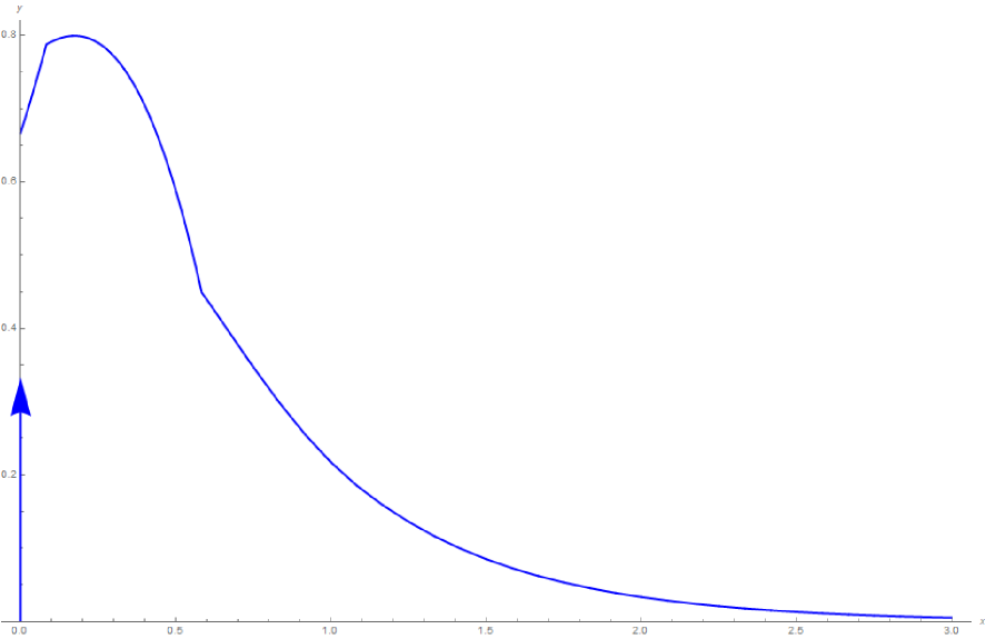
Figure 1: Waiting time density plot $y=f(x)$ for Uniform[$\frac{1}{12},\frac{7}{12}$] service.

pictured in Figure 1, where $\left\lfloor y\right\rfloor$ denotes the greatest integer $\leq y$.

Let us illustrate in greater detail:

$$i_{0}(x)=4{\displaystyle\int\limits_{-\infty}^{x-\frac{1}{12}}}\tfrac{2}{3}\exp(2\,t)dt=\tfrac{4}{3}\exp\left(-\tfrac{1}{6}+2x\right)$$

thus

$$\begin{array}[c]{ccc}f_{1}^{\prime}(x)=2f_{1}(x)-i_{0}(x),&&f_{1}\left(\tfrac{1}{12}\right)=f_{0}\left(\tfrac{1}{12}\right)=\tfrac{2}{3}\exp(\tfrac{1}{6})\end{array}$$

implying

$$f_{1}(x)=\tfrac{2}{3}\exp\left(2x\right)+\tfrac{1}{9}\exp\left(-\tfrac{1}{6}+2x\right)-\tfrac{4}{3}\exp\left(-\tfrac{1}{6}+2x\right)x.$$

Continuing:

$$i_{1}(x) =4{\displaystyle\int\limits_{\frac{1}{12}}^{x-\frac{1}{12}}}\left[\tfrac{2}{3}\exp\left(2t\right)+\tfrac{1}{9}\exp\left(-\tfrac{1}{6}+2t\right)-\tfrac{4}{3}\exp\left(-\tfrac{1}{6}+2t\right)t\right]dt$$

$$=-\tfrac{4}{3}-\tfrac{4}{3}\exp(\tfrac{1}{6})+\tfrac{16}{9}\exp\left(-\tfrac{1}{3}+2x\right)+\tfrac{4}{3}\exp\left(-\tfrac{1}{6}+2x\right)-\tfrac{8}{3}\exp\left(-\tfrac{1}{3}+2x\right)x,$$

$$j_{0}=4{\displaystyle\int\limits_{-\infty}^{\frac{1}{12}}}\tfrac{2}{3}\exp(2\,t)dt=\tfrac{4}{3}\exp(\tfrac{1}{6})$$

thus

$$\begin{array}[c]{ccc}f_{2}^{\prime}(x)=2f_{2}(x)-i_{1}(x)-j_{0},&&f_{2}\left(\tfrac{1}{6}\right)=f_{1}\left(\tfrac{1}{6}\right)=-\tfrac{1}{9}\exp(\tfrac{1}{6})+\tfrac{2}{3}\exp(\tfrac{1}{3})\end{array}$$

implying

$$f_{2}(x) =-\tfrac{2}{3}+\tfrac{2}{3}\exp(2x)+\tfrac{25}{27}\exp\left(-\tfrac{1}{3}+2x\right)+\tfrac{1}{9}\exp\left(-\tfrac{1}{6}+2x\right)$$

$$-\tfrac{16}{9}\exp\left(-\tfrac{1}{3}+2x\right)x-\tfrac{4}{3}\exp\left(-\tfrac{1}{6}+2x\right)x+\tfrac{4}{3}\exp\left(-\tfrac{1}{3}+2x\right)x^{2}.$$

The pattern is maintained:

$$f_{3}^{\prime}(x)=2f_{3}(x)-i_{2}(x)-j_{1}-j_{0},$$

$$f_{4}^{\prime}(x)=2f_{4}(x)-i_{3}(x)-j_{2}-j_{1}-j_{0},$$

$$f_{5}^{\prime}(x)=2f_{5}(x)-i_{4}(x)-j_{3}-j_{2}-j_{1}-j_{0},$$

$$f_{6}^{\prime}(x)=2f_{6}(x)-i_{5}(x)-j_{4}-j_{3}-j_{2}-j_{1}-j_{0}$$

until $x>\frac{7}{12}$ (the equation length becomes fixed and $k$ replaces the rightmost $j$):

$$f_{7}^{\prime}(x)=2f_{7}(x)-i_{6}(x)-j_{5}-j_{4}-j_{3}-j_{2}-j_{1}-k_{0}(x),$$

$$f_{8}^{\prime}(x)=2f_{8}(x)-i_{7}(x)-j_{6}-j_{5}-j_{4}-j_{3}-j_{2}-k_{1}(x),$$

$$f_{9}^{\prime}(x)=2f_{9}(x)-i_{8}(x)-j_{7}-j_{6}-j_{5}-j_{4}-j_{3}-k_{2}(x),$$

$$f_{10}^{\prime}(x)=2f_{10}(x)-i_{9}(x)-j_{8}-j_{7}-j_{6}-j_{5}-j_{4}-k_{3}(x).$$

We count $n(n+5)/2$ terms in each $f_{n}(x)$ upon expansion, at least for $1\leq n\leq 35$.

When numerically evaluating large symbolic expressions, it is important to ensure that the working precision of floating point quantities is suitably high. To evaluate $f(2)$ may require several hundred decimal digits because, for instance, the first two of the 348 numerator terms comprising $f_{24}(x)$ are

$$-31343712612206064875238458599056650210472221756256360\,\exp(4)$$

$$+1235688973308606091819588575256480179309880006812893184\,\exp(2x)$$

$$\approx(-1.7113\times 10^{54})+(6.7466\times 10^{55})$$

upon setting $x=2$.  The subtraction of nearly equal numbers, such as these, will lead to a horrific loss of precision unless appropriate care is taken.

2 Case Two ($0=a<b$)

Set $a=0$, $b=\frac{2}{3}$ and

$$g_{0}(x)=\tfrac{1}{6}\exp(x)\left[4\cos\left(\sqrt{2}x\right)-\sqrt{2}\sin\left(\sqrt{2}x\right)\right].$$

A sequence of functions is defined iteratively as follows:

$$g_{n}^{\prime\prime}(x)=2g_{n}^{\prime}(x)-3g_{n}(x)+3g_{n-1}\left(x-\tfrac{2}{3}\right),$$

$$\begin{array}[c]{ccc}g_{n}\left(\tfrac{2n}{3}\right)=g_{n-1}\left(\tfrac{2n}{3}\right),&&g_{n}^{\prime}\left(\tfrac{2n}{3}\right)=\delta_{n-1}+g_{n-1}^{\prime}\left(\tfrac{2n}{3}\right)\end{array}$$

where $\delta_{m}$ is the Kronecker delta.  Stitching the fragments together gives rise to

$$g(x)=g_{\left\lfloor\frac{3x}{2}\right\rfloor}(x)$$

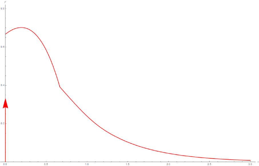
Figure 2: Waiting time density plot $y=g(x)$ for Uniform[$0,\frac{2}{3}$] service.

pictured in Figure 2.

Let us illustrate in greater detail:

$$g_{0}^{\prime}(x)=\tfrac{1}{6}\exp(x)\left[2\cos\left(\sqrt{2}x\right)-5\sqrt{2}\sin\left(\sqrt{2}x\right)\right]$$

thus

$$g_{1}^{\prime\prime}(x)=2g_{1}^{\prime}(x)-3g_{1}(x)+3g_{0}\left(x-\tfrac{2}{3}\right),$$

$$\begin{array}[c]{ccc}g_{1}\left(\tfrac{2}{3}\right)=g_{0}\left(\tfrac{2}{3}\right),&&g_{1}^{\prime}\left(\tfrac{2}{3}\right)=1+g_{0}^{\prime}\left(\tfrac{2}{3}\right)\end{array}$$

implying

$$g_{1}(x) =\tfrac{1}{6}\exp(x)\left[4\cos\left(\sqrt{2}x\right)-\sqrt{2}\sin\left(\sqrt{2}x\right)\right]$$

$$-\tfrac{1}{24}\exp\left(-\tfrac{2}{3}+x\right)\left[4\cos\left(\sqrt{2}\left(-\tfrac{2}{3}+x\right)\right)-\sqrt{2}\sin\left(\sqrt{2}\left(-\tfrac{2}{3}+x\right)\right)\right]$$

$$+\tfrac{1}{4}\exp\left(-\tfrac{2}{3}+x\right)\left[\cos\left(\sqrt{2}\left(-\tfrac{2}{3}+x\right)\right)+2\sqrt{2}\sin\left(\sqrt{2}\left(-\tfrac{2}{3}+x\right)\right)\right]x.$$

Beyond this point, the derivatives at $x=\frac{2n}{3}$ match:

$$g_{1}^{\prime}(x) =\tfrac{1}{6}\exp(x)\left[2\cos\left(\sqrt{2}x\right)-5\sqrt{2}\sin\left(\sqrt{2}x\right)\right]$$

$$+\tfrac{1}{24}\exp\left(-\tfrac{2}{3}+x\right)\left[4\cos\left(\sqrt{2}\left(-\tfrac{2}{3}+x\right)\right)+17\sqrt{2}\sin\left(\sqrt{2}\left(-\tfrac{2}{3}+x\right)\right)\right]$$

$$+\tfrac{1}{4}\exp\left(-\tfrac{2}{3}+x\right)\left[5\cos\left(\sqrt{2}\left(-\tfrac{2}{3}+x\right)\right)+\sqrt{2}\sin\left(\sqrt{2}\left(-\tfrac{2}{3}+x\right)\right)\right]x$$

thus

$$g_{2}^{\prime\prime}(x)=2g_{2}^{\prime}(x)-3g_{2}(x)+3g_{1}\left(x-\tfrac{2}{3}\right),$$

$$\begin{array}[c]{ccc}g_{2}\left(\tfrac{4}{3}\right)=g_{1}\left(\tfrac{4}{3}\right),&&g_{2}^{\prime}\left(\tfrac{4}{3}\right)=g_{1}^{\prime}\left(\tfrac{4}{3}\right)\end{array}$$

implying

$$g_{2}(x) =\tfrac{1}{6}\exp(x)\left[4\cos\left(\sqrt{2}x\right)-\sqrt{2}\sin\left(\sqrt{2}x\right)\right]$$

$$-\tfrac{1}{24}\exp\left(-\tfrac{2}{3}+x\right)\left[4\cos\left(\sqrt{2}\left(-\tfrac{2}{3}+x\right)\right)-\sqrt{2}\sin\left(\sqrt{2}\left(-\tfrac{2}{3}+x\right)\right)\right]$$

$$+\tfrac{1}{4}\exp\left(-\tfrac{2}{3}+x\right)\left[\cos\left(\sqrt{2}\left(-\tfrac{2}{3}+x\right)\right)+2\sqrt{2}\sin\left(\sqrt{2}\left(-\tfrac{2}{3}+x\right)\right)\right]x$$

$$-\tfrac{1}{192}\exp\left(-\tfrac{4}{3}+x\right)\left[8\cos\left(\sqrt{2}\left(-\tfrac{4}{3}+x\right)\right)-29\sqrt{2}\sin\left(\sqrt{2}\left(-\tfrac{4}{3}+x\right)\right)\right]$$

$$+\tfrac{1}{32}\exp\left(-\tfrac{4}{3}+x\right)\left[17\cos\left(\sqrt{2}\left(-\tfrac{4}{3}+x\right)\right)-2\sqrt{2}\sin\left(\sqrt{2}\left(-\tfrac{4}{3}+x\right)\right)\right]x$$

$$-\tfrac{3}{32}\exp\left(-\tfrac{4}{3}+x\right)\left[4\cos\left(\sqrt{2}\left(-\tfrac{4}{3}+x\right)\right)-\sqrt{2}\sin\left(\sqrt{2}\left(-\tfrac{4}{3}+x\right)\right)\right]x^{2}.$$

3 Case Three ($0<a=b$)

Set $a=b=\frac{1}{3}$ and

$$h_{0}(x)=\tfrac{2}{3}\exp(2\,x).$$

A sequence of functions is defined iteratively as follows:

$$h_{n}^{\prime}(x)=2h_{n}(x)-2h_{n-1}\left(x-\tfrac{1}{3}\right),$$

$$h_{n}\left(\tfrac{n}{3}\right)=-\tfrac{2}{3}\delta_{n-1}+h_{n-1}\left(\tfrac{n}{3}\right).$$

The role of $\delta_{m}$ here is more pronounced than in Section 2: a jump discontinuity occurs in the density at $x=\frac{1}{3}$ (as opposed to merely a sharp corner) .  Stitching the fragments together gives rise to

$$h(x)=h_{\left\lfloor 3x\right\rfloor}(x)$$

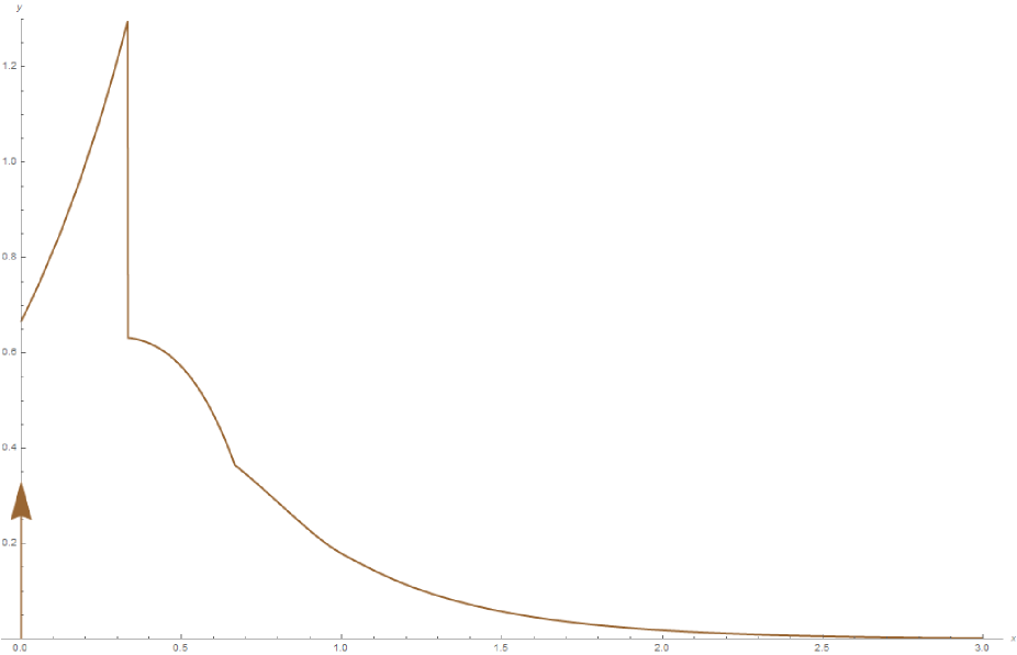
Figure 3: Waiting time density plot $y=h(x)$ for Deterministic[$\frac{1}{3}$] service.

pictured in Figure 3.

We could do as before, indicating steps leading to $h_{1}(x)$ and $h_{2}(x)$. A classical result due to Erlang [6, 7, 8, 9]:

$$h_{n}(x)=\left(1-\rho\right)\frac{d}{dx}\left\{{\displaystyle\sum\limits_{m=0}^{n}}(-1)^{m}\frac{\lambda^{m}\left(x-a\,m\right)^{m}}{m!}\exp\left[\lambda(x-a\,m)\right]\right\}$$

renders this listing unnecessary (with $1-\rho=\frac{1}{3}$, $\lambda=2$, $a=\frac{1}{3}$).  We wonder if such a formula (for the M/D/1 queue) possesses an analog for the M/U/1 queue.

4 Personal Notes

I taught a semester-long class in statistical programming at Harvard University (as a preceptor) for nearly ten years.  A favorite set of problems began with an M/M/1 example [10] involving a hospital emergency room (ER).

Patients (clients) arrive according to a Poisson process with rate $\lambda$.  One doctor (server) is available to treat them.  The doctor, when busy, treats patients with rate $\mu$.  More precisely: interarrival times are exponentially distributed with mean $1/\lambda$ and treatment lengths are exponentially distributed with mean $1/\mu$.  The ER is open 24 hours a day, 7 days a week.  Patients must wait until the doctor is free and are treated in the order via which they arrive.  Simulate the performance of the ER over many weeks.  What can be said about waiting time in queue per patient (excluding service time)?  Determine the mean, variance, mode and median of $W_{\text{que}}$ to as high accuracy as possible.  Assume for this purpose that the expected number of arriving patients per hour is $\lambda=2$ and that the expected number of treatment completions per hour (for a continuously busy ER) is $\mu=3$.

Putting aside experiment in favor of pristine theory, the Laplace transform of service density $\mu\exp(-\mu\,x)$ is $\mu/(\mu+s)$.  Formulas for the mean and variance of $W_{\text{que}}$ follow immediately from

$$F(s)=\frac{(1-\rho)s}{s-\lambda+\lambda\frac{\mu}{\mu+s}};$$

consequently

$$\begin{array}[c]{ccc}\text{mean}=-F^{\prime}(0)=\dfrac{\lambda}{\mu(\mu-\lambda)},&&\text{variance}=F^{\prime\prime}(0)-F^{\prime}(0)^{2}=\dfrac{\lambda(2\mu-\lambda)}{\mu^{2}(\mu-\lambda)^{2}}\end{array}$$

giving $\frac{2}{3}$ and $\frac{8}{9}$ respectively.  An expression for the density of $W_{\text{que}}$:

$$f(x)=(1-\rho)\delta(x)+\rho(\mu-\lambda)\exp(-(\mu-\lambda)x)$$

shows that the mode is $0$; integrating and solving the equation

$$1-\rho-\rho\left[\exp(-(\mu-\lambda)x)-1\right]=\dfrac{1}{2}$$

implies

$$\begin{array}[c]{ccccc}\dfrac{1}{2}=\rho\exp(-(\mu-\lambda)x),&&\text{i.e.,}&&x=\dfrac{1}{\mu-\lambda}\ln\left(\dfrac{2\lambda}{\mu}\right)\end{array}$$

giving the median to be $\ln(4/3)=0.28768207...$.

The aforementioned problem set continued with an M/G/1 example, involving the same ER parameters, but with Uniform[$a,b$] treatment lengths.  Since $1/3=(a+b)/2$ was required, I arbitrarily chose $a=1/12$ and $b=7/12$.

Perform exactly the same simulation as before, except assume treatment lengths (in minutes) are uniformly distributed on the interval $[5,35]$.  Less is known about this scenario than the preceding (with exponential service times).

The thought of choosing $(a,b)=(0,2/3)$ or $(1/3,1/3)$ did not occur to me until later.  I had imagined that numerical inversion of Laplace transforms was the only avenue available to reliably estimate the mode and median.

Just as $(a+b)/2$ is the first moment of treatment lengths,

$$\begin{array}[c]{ccc}\xi=\dfrac{a^{2}+a\,b+b^{2}}{3},&&\eta=\dfrac{(a+b)\left(a^{2}+b^{2}\right)}{4}\end{array}$$

are the corresponding second and third moments.  Again, favoring pristine theory over experiment,

$$F(s)=\frac{(1-\rho)s}{s-\lambda+\lambda\tfrac{\exp(-a\,s)-\exp(-b\,s)}{(b-a)s}};$$

consequently [11, 12]

$$\begin{array}[c]{ccc}\text{mean}=-F^{\prime}(0)=\dfrac{\lambda\,\xi}{2(1-\rho)},&&\text{variance}=F^{\prime\prime}(0)-F^{\prime}(0)^{2}=\dfrac{\lambda\,\eta}{3(1-\rho)}+\dfrac{\lambda^{2}\xi^{2}}{4(1-\rho)^{2}}\end{array}$$

giving $\frac{19}{48}$ and $\frac{1883}{6912}$ respectively.  The mode (location of the density maximum, excluding $0$) occurs when

$$f_{2}^{\prime}(x_{0})=0$$

i.e.,

$$x_{0}=\tfrac{1}{6}\left(1+3e^{1/6}-\sqrt{3e^{1/6}\left(7-3e^{1/6}\right)}\right)=0.17405980...;$$

solving the equation

$${\displaystyle\int\limits_{c_{0}}^{c_{1}}}f_{0}(t)dt+{\displaystyle\int\limits_{c_{1}}^{c_{2}}}f_{1}(t)dt+{\displaystyle\int\limits_{c_{2}}^{x}}f_{2}(t)dt=\tfrac{1}{2}$$

gives the median to be $0.21673428...$.

My classroom example deviates from the direction of research [13], which emphasizes heavy-tailed service time distributions.  Ramsay [14] discovered a remarkably compact formula – a single integral of a non-oscillating function over the real line – in connection with Pareto service times.  My formulas for uniform service times are sprawling by comparison.

The recursive solution of delay-differential equations is certainly not new [15] but application of such to queueing theory does not seem to be widespread.  Counterexamples include [16, 17]; surely there are more that I’ve missed.  Symbolics are mentioned in [13].

The waiting time probability for M/D/1 seems to decay exponentially (as do the other two cases).  The Cramér-Lundberg approximation [18] is applicable; alternatively, we have asymptotics [11, 19]

$$\begin{array}[c]{ccc}\operatorname*{P}\left\{W_{\text{que}}>x\right\}\sim\dfrac{1-\rho}{\tau\,\rho-1}\exp\left[-\lambda(\tau-1)x\right]&&\text{as }x\rightarrow\infty\text{ }\end{array}$$

where $\tau>1$ is the unique root of $\tau\exp\left[-\rho(\tau-1)\right]=1$.

Returning finally to M/U/1, let $L_{\text{sys}}$ denote the number of patients in the system (both queue and service).  Define

$$\begin{array}[c]{ccc}\tilde{F}(z)=\dfrac{(1-\rho)(1-z)\Theta(\lambda(1-z))}{\Theta(\lambda(1-z))-z},&&\sigma^{2}=\xi-\dfrac{1}{\mu^{2}}.\end{array}$$

Under equilibrium, with $\lambda=2$, $\mu=3$ and $a=\frac{1}{12}$, $b=\frac{7}{12}$, we have

$$\tilde{f}(\ell)=\mathbb{P}\left\{L_{\text{sys}}=\ell\right\}=\frac{1}{\ell!}\left.\frac{d^{\ell}\tilde{F}}{dz^{\ell}}\right|_{z=0}=\left\{\begin{array}[c]{lll}\frac{1}{3}=0.333333...&&\text{if }\ell=0\\ \frac{1-e+e^{7/6}}{-3+3e}=0.289628...&&\text{if }\ell=1\\ 0.177042...&&\text{if }\ell=2\\ 0.096164...&&\text{if }\ell=3\\ 0.050209...&&\text{if }\ell=4\\ 0.025950...&&\text{if }\ell=5\end{array}\right.;$$

consequently [20, 21]

$$\text{mean}=\tilde{F}^{\prime}(1)=\rho+\dfrac{\rho^{2}+\lambda^{2}\sigma^{2}}{2(1-\rho)},$$

variance $$=\tilde{F}^{\prime\prime}(1)+\tilde{F}^{\prime}(1)-\tilde{F}^{\prime}(1)^{2}$$

$$=\rho(1-\rho)+\dfrac{(3-2\rho)(\rho^{2}+\lambda^{2}\sigma^{2})}{2(1-\rho)}+\dfrac{(\rho^{2}+\lambda^{2}\sigma^{2})^{2}}{4(1-\rho)}+\frac{\lambda^{3}\eta}{3(1-\rho)}+\frac{\lambda^{4}\rho\,\xi^{2}}{4(1-\rho)^{2}}$$

giving $\frac{35}{24}$ and $\frac{4547}{1728}$ respectively.  The final term for the variance is missing in [21].  The probability generating function $\tilde{f}(\ell)$ seems to decay geometrically, but details surrounding the exact limit of successive ratios have not been verified [20].

I am grateful to innumerable software developers, as my “effective” formulas are too lengthy to be studied in any traditional sense.  Mathematica routines NDSolve for DDEs and InverseLaplaceTransform (for Mma version $\geq 12.2$) plus ILTCME [22] assisted in numerically confirming many results.  R steadfastly remains my favorite statistical programming language.  A student asked in 2006 for my help in writing a relevant R simulation, leading to the computational exercises described here and to my abiding interest in queues [23, 24].

5 Addendum

For completeness, another M/D/1 result is provided. Under equilibrium, with $\lambda=2$, $\mu=3$ and $a=\frac{1}{3}=b$, we have

$$\tilde{h}(\ell)=\mathbb{P}\left\{L_{\text{sys}}=\ell\right\}=\left\{\begin{array}[c]{lll}\frac{1}{3}=0.333333...&&\text{if }\ell=0\\ \frac{-1+e^{2/3}}{3}=0.315911...&&\text{if }\ell=1\\ \frac{-5e^{2/3}+3e^{4/3}}{9}=0.182481...&&\text{if }\ell=2\\ \frac{8e^{2/3}-21e^{4/3}+9e^{2}}{27}=0.089494...&&\text{if }\ell=3\\ \frac{-22e^{2/3}+180e^{4/3}-243e^{2}+81e^{8/3}}{243}=0.042035...&&\text{if }\ell=4\\ \frac{14e^{2/3}-312e^{4/3}+972e^{2}-891e^{8/3}+243e^{10/3}}{729}=0.019607...&&\text{if }\ell=5\end{array}\right.;$$

giving $\frac{4}{3}$ and $\frac{56}{27}$ for the mean and variance, yet unverified limit of successive ratios.

References

[1]J. F. Shortle, J. M. Thompson, D. Gross and C. M. Harris,
Fundamentals of Queueing Theory, 5 ed., Wiley, 2018,
pp. 261–268, 271–275, 443–444; MR3791493.
[2]M. F. Neuts, Generalizations of the Pollaczek-Khinchin
integral equation in the theory of queues, Adv. in Appl. Probab. 18
(1986) 952–990; MR0867095.
[3]K. H. Lundberg, H. R. Miller and D. L. Trumper, Initial
conditions, generalized functions, and the Laplace transform troubles at the
origin, IEEE Control Systems Magazine 27 (2007) 22–35.
[4]J. L. Schiff, The Laplace Transform: Theory and
Applications, Springer-Verlag, 1999, pp. 88–89; MR1716143.
[5]A. Henderson, Extension of the initial value theorem,
Internat. J. Electrical Engineering & Education 15 (1978) 237–241.
[6]A. K. Erlang, The theory of probabilities and telephone
conversations (in Danish), Nyt Tidsskrift for Matematik 20B (1909)
33–39; Engl. transl. in E. Brockmeyer, H. L. Halstrøm and A. Jensen, eds.,
The Life and Works of A. K. Erlang, Trans. Danish Acad. Tech. Sci.,
1948, pp. 131-137; MR0027976.
[7]V. B. Iversen and L. Staalhagen, Waiting time distribution
in M/D/1 queueing systems, Electronics Letters 35 (1999) 2184–2185.
[8]N. U. Prabhu, Stochastic Storage Processes. Queues,
Insurance Risk, Dams, and Data Communication, 2 ed.,
Springer-Verlag, 1998, pp. 36–37, 75–78; MR1492990.
[9]H. Tijms, New and old results for the M/D/c queue,
AEU - Internat. J. Electronics and Communications 60 (2006) 125–130.
[10]F. S. Hillier and G. J. Lieberman, Introduction to
Operations Research, 3 ed., Holden-Day, 1980, pp. 400–457
(chapter entitled “Queueing Theory”); MR0569591.
[11]H. C. Tijms, A First Course in Stochastic Models,
Wiley, 2003, pp. 327–331, 348–353, 381–384; MR2190630.
[12]X. Zhao, J. Hou and K. Gilbert, Measuring the variance of
customer waiting time in service operations, Management Decision 52
(2014) 296–312.
[13]J. F. Shortle, P. H. Brill, M. J. Fischer, D. Gross and D.
M. B. Masi, An algorithm to compute the waiting time distribution for the
M/G/1 queue, INFORMS J. Comput. 16 (2004) 152–161; MR2065995.
[14]C. M. Ramsay, Exact waiting time and queue size
distributions for equilibrium M/G/1 queues with Pareto service,
Queueing Systems 57 (2007) 147–155; MR2369214.
[15]S. R. Finch, Components and cycles of random mappings, arXiv:2205.05579.
[16]M. Vlasiou, Lindley-Type Recursions, Ph.D. thesis,
Eindhoven University of Technology, 2006, http://research.tue.nl/en/publications/lindley-type-recursions.
[17]O. J. Boxma and M. Vlasiou, On queues with service and
interarrival times depending on waiting times, Queueing Systems 56
(2007) 121–132; arXiv:1404.5549; MR2336100.
[19]H. Tijms and K. Staats, Negative probabilities at work in
the M/D/1 queue, Probab. Engrg. Inform. Sci. 21 (2007) 67–76; MR2289220.
[20]M. L. Chaudhry, U. C. Gupta and M. Agarwal, Exact and
approximate numerical solutions to steady-state single-server queues: M/G/1 –
a unified approach, Queueing Systems 10 (1992) 351–379; MR1150007.
[21]J. D. Griffiths, The coefficient of variation of queue size
for heavy traffic, J. Operational Research Society 47 (1996) 1071-1076.
[22]G. Horváth, I. Horváth, M. Telek, S. Al-Deen Almousa
and Z. Talyigás, Inverse Laplace Transform with Concentrated
Matrix-Exponential Functions, http://inverselaplace.org.
[23]S. Finch, M/D/1 queues with LIFO and SIRO policies, arXiv:2208.09980.
[24]S. Finch, D/M/1 queue: Policies and control, arXiv:2210.08545.