OpenXAI: Towards a Transparent Evaluation of
Post hoc Model Explanations

Abstract

While several types of post hoc explanation methods have been proposed in recent literature, there is very little work on systematically benchmarking these methods. Here, we introduce OpenXAI, a comprehensive and extensible open-source framework for evaluating and benchmarking post hoc explanation methods. OpenXAI comprises of the following key components: (i) a flexible synthetic data generator and a collection of diverse real-world datasets, pre-trained models, and state-of-the-art feature attribution methods, (ii) open-source implementations of twenty-two quantitative metrics for evaluating faithfulness, stability (robustness), and fairness of explanation methods, and (iii) the first ever public XAI leaderboards to readily compare several explanation methods across a wide variety of metrics, models, and datasets. OpenXAI is easily extensible, as users can readily evaluate custom explanation methods and incorporate them into our leaderboards.

Overall, OpenXAI provides an automated end-to-end pipeline that not only simplifies and standardizes the evaluation of post hoc explanation methods, but also promotes transparency and reproducibility in benchmarking these methods. While the first release of OpenXAI supports only tabular datasets, the explanation methods and metrics that we consider are general enough to be applicable to other data modalities. OpenXAI datasets and data loaders, implementations of state-of-the-art explanation methods and evaluation metrics, as well as leaderboards are publicly available at https://open-xai.github.io/. OpenXAI will be regularly updated to incorporate text and image datasets, other new metrics and explanation methods, and welcomes inputs from the community.

1 Introduction

As predictive models are increasingly deployed in critical domains (e.g., healthcare, law, and finance), there has been a growing emphasis on explaining the predictions of these models to decision makers (e.g. doctors, judges) so that they can understand the rationale behind model predictions, and determine if and when to rely on these predictions. To this end, various techniques have been proposed in recent literature to generate post hoc explanations of individual predictions made by complex ML models. Several of such local explanation methods output the influence of each of the features on the model’s prediction, and are therefore referred to as local feature attribution methods. Due to their generality, feature attribution methods are increasingly being utilized to explain complex models in medicine, finance, law, and science [23, 34, 78]. Thus, it is critical to ensure that the explanations generated by these methods are reliable so that relevant stakeholders and decision makers are provided with credible information about the underlying models [6].

Prior works have studied several notions of explanation reliability such as faithfulness (or fidelity) [81, 51, 33], stability (or robustness) [7, 4], and fairness [18, 9], and proposed metrics for quantifying these notions. Many of these works also demonstrated through small-scale experiments or qualitative analysis that certain explanation methods are not effective w.r.t. specific notions of reliability. For instance, Alvarez-Melis and Jaakkola [7] visualized the explanations generated by some of the popular gradient based explanation methods  [67, 66, 70, 72] for MNIST images, and showed that they are not robust to small input perturbations. However, it is unclear if such findings generalize beyond the settings studied. More broadly, one of the biggest open questions which has far-reaching implications for the progress of explainable AI (XAI) research is: which explanation methods are effective w.r.t. what notions of reliability and under what conditions?  [43]. A first step towards answering this question involves systematically benchmarking explanation methods in a reproducible and transparent manner. However, the increasing diversity of explanation methods, and the plethora of evaluation settings and metrics outlined in existing research without standardized open-source implementations make it rather challenging to carry out such benchmarking efforts.

In this work, we address the aforementioned challenges by introducing OpenXAI, a comprehensive and extensible open-source framework for systematically and efficiently benchmarking explanation methods in a transparent and reproducible fashion. More specifically, our work makes the following key contributions:

1. We introduce the OpenXAI framework, an open-source ecosystem designed to support systematic, reproducible, and efficient evaluations of post hoc explanation methods. OpenXAI unifies the existing scattered repositories of datasets, models, and evaluation metrics, and provides a simple and easy-to-use API that enables researchers and practitioners to benchmark explanation methods using just a few lines of code (Section 2).

2. Our OpenXAI framework currently provides open-source implementations and ready-to-use API interfaces for seven state-of-the-art feature attribution methods (LIME, SHAP, Vanilla Gradients, Gradient x Input, SmoothGrad, and Integrated Gradients), and twenty-two quantitative metrics to evaluate the faithfulness, stability, and fairness of feature attribution methods. In addition, it includes a comprehensive collection of seven real-world datasets spanning diverse real-world domains, and sixteen different pre-trained models. OpenXAI also introduces a novel and flexible synthetic data generator to synthesize datasets of varying sizes, complexity, and dimensionality which facilitate the construction of reliable ground truth explanations (Section 2).

3. As part of our OpenXAI framework, we also develop the first-ever public XAI leaderboards (shown in Figure 1) to promote transparency, and to allow users to easily compare the performance of multiple explanation methods across a wide variety of synthetic and real-world datasets, evaluation metrics, and predictive models.

4. OpenXAI framework is easily extensible i.e., researchers and practitioners can readily incorporate custom explanation methods, datasets, predictive models, and evaluation metrics into our framework and leaderboards (Section 2).

5. Lastly, using our proposed OpenXAI framework, we perform rigorous empirical benchmarking of the aforementioned state-of-the-art feature attribution methods to determine which methods are effective w.r.t. what notions of reliability across a wide variety of datasets and predictive models (Section 3).

Overall, our OpenXAI framework provides an end-to-end pipeline that unifies, simplifies, and standardizes several existing workflows to evaluate explanation methods. By enabling systematic and efficient evaluation and benchmarking of existing and new explanation methods, our OpenXAI framework can inform and accelerate new research in the emerging field of XAI. OpenXAI will be regularly updated and welcomes input from the community.

Related Work. Our work builds on the vast literature in explainable AI. Here, we discuss closely related works and their connections to our benchmark. A more detailed discussion of the related work is included in the Appendix.

Evaluation Metrics for Post hoc Explanations: Prior research has studied several notions of explanation reliability, namely, faithfulness (or fidelity), stability (or robustness), and fairness [51, 81, 7, 18]. While the faithfulness notion captures how faithfully a given explanation captures the true behavior of the underlying model [81, 51, 33], stability ensures that explanations do not change drastically with small perturbations to the input [29, 7]. The fairness notion, on the other hand, ensures that there are no group-based disparities in the faithfulness or stability of explanations [18]. To this end, prior works [51, 69, 81, 7, 18, 33] proposed various evaluation metrics to quantify the aforementioned notions. For instance, Petsiuk et al. [59] measured the change in the probability of the predicted class when important features (as identified by an explanation) are deleted from or introduced into the data instance. A sharp change in the probability implies a high degree of explanation faithfulness. Alvarez-Melis and Jaakkola [7] loosely quantified stability as the maximum change in the resulting explanations when small perturbations are made to a given instance. Dai et al. [18] quantified unfairness of explanations as the difference between the faithfulness (or stability) metric values averaged over instances in the majority and the minority subgroups.

XAI Libraries and Benchmarks: Prior works have introduced a few XAI libraries and benchmarks, the most popular among them being Captum [42], Quantus [32], XAI-Bench [51], and SHAP Benchmark. Below, we provide a brief description of each of these, and detail how our work differs from them.

While Captum library [42] is an open-source library which provides implementations and APIs for various state-of-the-art explanation methods, its focus is not on evaluating and/or benchmarking these methods which is the main goal of our work. Quantus library [32], on the other hand, provides implementations of certain evaluation metrics to measure the faithfulness and stability/robustness of explanation methods. However, it does not focus on benchmarking explanation methods or providing public dashboards to compare the performance of these methods. Furthermore, the stability/robustness measures [7] supported by Quantus are somewhat outdated and have been superseded by recently proposed metrics [4]. In addition, Quantus does not support any fairness metrics to evaluate disparities in the quality of explanations which is very important in real-world settings such as healthcare, criminal justice, and policy. In contrast, OpenXAI not only subsumes popular faithfulness and stability/robustness metrics supported by Quantus but also supports 19 new metrics to measure the faithfulness, stability/robustness, as well as the fairness of explanation methods [4, 18, 43]. In addition, OpenXAI focuses on systematically benchmarking state-of-the-art explanation methods and providing public dashboards to readily compare these methods.

SHAP benchmark [2] only focuses on evaluating and comparing different variants of SHAP [54] via certain faithfulness metrics which are similar to the Prediction Gap on Important (PGI) and Unimportant (PGU) feature perturbation metrics outlined in our work. Note that the SHAP benchmark does not include any stability/robustness or fairness metrics. In contrast, OpenXAI not only includes 20 new metrics to evaluate the stability/robustness and fairness of explanation methods but also benchmarks various other methods (e.g., LIME, Gradient-based methods).

XAI-Bench [51] constructed synthetic datasets with ground truth explanations to evaluate the faithfulness of a few explanation methods (e.g., LIME, SHAP, MAPLE). However, recent research argued that their evaluation is unreliable, and predictive models learned using their synthetic datasets may not adhere to the ground truth explanations [24]. In addition, the aforementioned evaluation is rather limited in scope as synthetic datasets may not even be representative of real-world data [24]. In contrast, our work not only proposes a novel synthetic data generator that addresses the shortcomings of the synthetic datasets constructed in XAI-Bench but also facilitates the evaluation and benchmarking of the faithfulness, stability, as well as the fairness of 7 state-of-the-art explanation methods on 7 real-world datasets with no ground truth explanations.

In summary, our work is significantly different from existing libraries and benchmarks, and makes the following key contributions:

• We provide implementations and easy-to-use API interfaces for 22 metrics to evaluate the faithfulness, stability, and fairness of explanation methods. 18 out of the 22 state-of-the-art metrics included in OpenXAI have not been implemented in any prior libraries or benchmarks – e.g., faithfulness metrics such as Feature Agreement (FA), Rank Agreement (RA), Sign Agreement (SA), Signed Rank Agreement (SRA), Pairwise Rank Agreement (PRA), stability metrics such as Relative Representation Stability (RRS), Relative Output Stability (ROS), and all fairness metrics.

• We also introduce a novel and flexible synthetic data generator to synthesize datasets of varying sizes, complexity, and dimensionality to facilitate the construction of reliable ground truth explanations in order to evaluate state-of-the-art explanation methods. Our synthetic data generator addresses the shortcomings of the prior synthetic benchmark (XAI-Bench) by generating synthetic datasets which encapsulate certain key properties, namely, unambiguously defined local neighborhoods, a clear description of feature importances in each local neighborhood, and feature independence. These properties, in turn, allow us to theoretically guarantee that any accurate model trained on our synthetic datasets will adhere to the ground truth explanations of the underlying data.

• We perform rigorous empirical benchmarking of 7 state-of-the-art feature attribution methods using our OpenXAI framework to determine which methods are effective w.r.t. each of the 22 evaluation metrics across 8 real-world and synthetic datasets, and 16 different predictive models. Note that none of the previously proposed libraries or benchmarks carry out such exhaustive benchmarking efforts across such a wide variety of metrics, models, and datasets. We also introduce the first ever public XAI leaderboards with such a wide variety of explanation methods, metrics, models, and datasets, to promote transparency and showcase the results of our benchmarking efforts.

2 Overview of OpenXAI Framework

OpenXAI provides a comprehensive programmatic environment with synthetic and real-world datasets, data processing functions, explainers, and evaluation metrics to rigorously and efficiently benchmark explanation methods. Below, we discuss each of these components in detail.

1) Datasets and Predictive Models. The current release of our OpenXAI framework includes a collection of eight different synthetic and real-world datasets. While synthetic datasets allow us to construct ground truth explanations which can then be used to evaluate explanations output by state-of-the-art methods, real-world datasets (where it is typically hard to construct ground truth explanations) help us benchmark these methods in a more realistic manner suitable for practical applications [51]. We would like to note that OpenXAI includes datasets that are widely employed in XAI research to evaluate the efficacy of newly proposed methods and study the behavior of existing methods [9, 18, 19, 20, 38, 69, 73].

Synthetic Datasets: While prior research [51, 41] proposed methods to generate synthetic datasets and corresponding ground truth explanations, they all suffer from a significant drawback as demonstrated by Faber et al. [24] – there is no guarantee that the models trained on these datasets will adhere to the ground truth explanations of the underlying data. This, in turn, implies that evaluating post hoc explanations using the above ground truth explanations would be incorrect since post hoc explanations are supposed to reliably explain the behavior of the underlying model, and not that of the underlying data. To illustrate, let us consider the case where we use aforementioned methods to construct a synthetic dataset with features $A,B,$ $C$, and $D$ such that the ground truth labels only depend on features $A$ and $B$ i.e., the ground truth explanation of the underlying data indicates that features $A$ and $B$ are most important. If we train a model on this data and if features $A$ and $B$ are correlated with $C$ and $D$ respectively, then the resulting model may base its predictions on $C$ and $D$ (and not $A$ and $B$) and still be very accurate. If a post hoc explanation of this model then (correctly) indicates that the most important features of the model are $C$ and $D$, this explanation may be deemed incorrect if we compare it against the ground truth explanation of the underlying data. This problem further exacerbates as we increase the complexity of the ground truth labeling function [24].

To address the aforementioned challenges, we develop a novel synthetic data generation mechanism, SynthGauss, which encapsulates three key properties, namely, feature independence, unambiguously-defined local neighborhoods, and a clear description of feature influence in each local neighborhood. Intuitively, this approach generates $K$ well-separated clusters where points in each cluster $k\in\{1,2,\cdots,K\}$ are sampled from a Gaussian distribution $\mathcal{N}(\mu_{k},\Sigma_{k})$ where $u_{k}\in R^{d}$ is the mean and $\Sigma_{k}\in R^{d\times d}$ is the covariance matrix. While this parameterization is general enough to support the construction of synthetic datasets of $K$ clusters with varying means and covariances, we set the means of all the clusters such that the intracluster distances are significantly smaller than the intercluster distances, and we set the covariance matrices of all the clusters to identity. This ensures that all the features are independent, and local neighborhoods (clusters) are unambiguously defined.

We then generate ground truth labels for instances by first randomly sampling feature mask vectors $m_{k}\in\{0,1\}^{d}$ (vectors comprising of 0s and 1s) for each cluster $k$. The vector $m_{k}$ determines which features influence the ground truth labeling process for instances in cluster $k$ (a value of 1 indicates that the corresponding feature is influential). We then randomly sample feature weight vectors $w_{k}\in R^{d}$ which capture the relative importance of each of the features in the labeling process of instances in each cluster $k$. The ground truth labels of instances in each cluster $k$ are then computed as a function (e.g., sigmoid) of the feature values of individual instances, and the dot product of the corresponding cluster’s feature mask vector and weight vector i.e., $m_{k}\odot w_{k}$. Complete pseudocode and other details of this generation process are included in the Appendix. Note that $m_{k}$ corresponds to the ground truth explanation for all instances in cluster $k$. Since our generation process is designed to encapsulate feature independence, unambiguous definitions of local neighborhoods, and clear descriptions of feature influences, any accurate model trained on the resulting dataset will adhere to the ground truth explanations of the underlying data (See Theorem 1 in Appendix).

Real-world Datasets: In the current release of OpenXAI, we include seven real-world datasets that are highly diverse in terms of several key properties. They comprise of data spanning multiple real-world domains (e.g., finance, lending, healthcare, and criminal justice), varying dataset sizes (e.g., small vs. large-scale), dimensionalities (e.g., low vs. high dimensional), class imbalance ratios, and feature types (e.g., continuous vs. discrete). We focus on tabular data in this release as such data is commonly encountered in real-world applications where explainability is critical [75], and has also been widely studied in XAI literature [51]. Table 1 provides a summary of the real-world datasets currently included in OpenXAI. See Section E.1 in the Appendix for detailed descriptions of individual datasets. While these real-world datasets are primarily drawn from prior research and existing repositories, OpenXAI provides comprehensive data loading and pre-processing capabilities to make these datasets XAI-ready (more details below). We also plan to expand our collection of real-world datasets in the next iteration. Adding a new dataset into our collection is as simple as uploading a .csv file or a .zip folder. Users can also submit requests to incorporate new datasets into the OpenXAI framework by filling a simple form and providing links to the datasets (See Appendix).

Table 1: Summary of currently available datasets in OpenXAI. Here, “feature types” denotes whether features in the dataset are discrete or continuous, “feature information” describes what kind of information is captured in the dataset, and “balanced” denotes whether the dataset is balanced w.r.t. the predictive label.

Dataset	Size	# features	Feature types	Feature information	Balanced
Synthetic Data	5,000	20	continuous	synthetic	✓
German Credit [22]	1,000	20	discrete, continuous	demographic, personal, financial	✗
HELOC [25]	9,871	23	continuous	demographic, financial	✓
COMPAS [36]	18,876	7	discrete, continuous	demographic, personal, criminal	✗
Adult Income [79]	48,842	13	discrete, continuous	demographic, personal, education/employment, financial	✗
Give Me Some Credit [27]	102,209	10	discrete, continuous	demographic, personal, financial	✗
Pima-Indians Diabetes [71]	768	9	discrete, continuous	demographic, healthcare	✗
Framingham heart study [1]	4,240	16	continuous	demographic, healthcare	✗

Data loaders and pre-trained models: OpenXAI provides a Dataloader class that can be used to load the aforementioned collection of synthetic and real-world datasets as well as any other custom datasets, and ensures that they are XAI-ready. More specifically, this class takes as input the name of an existing OpenXAI dataset or a new dataset (name of the .csv file), and outputs a train set which can then be used to train a predictive model, a test set which can be used to generate local explanations of the trained model, as well as any ground-truth explanations (if and when available). If the dataset already comes with pre-determined train and test splits, this class loads train and test sets from those pre-determined splits. Otherwise, it divides the entire dataset randomly into train (70%) and test (30%) sets. Users can also customize the percentages of train-test splits. The code snippet below shows how to import the Dataloader class and load an existing OpenXAI dataset. from OpenXAI import Dataloader
loader_train, loader_test = Dataloader.return_loaders(data_name=‘german’, download=True)
inputs, labels = iter(loader_test).next() We also pre-trained two classes of predictive models (e.g., deep neural networks of varying degrees of complexity, logistic regression models etc.) and incorporated them into the OpenXAI framework so that they can be readily used for benchmarking explanation methods. The code snippet below shows how to load OpenXAI’s pre-trained models using our LoadModel class. from OpenXAI import LoadModel
model = LoadModel(data_name=‘german’, ml_model=‘ann’) Adding additional pre-trained models into the OpenXAI framework is as simple as uploading a file with details about model architecture and parameters in a specific template. Users can also submit requests to incorporate custom pre-trained models into the OpenXAI framework by filling a simple form and providing details about model architecture and parameters (See Appendix).

2) Explainers. OpenXAI provides ready-to-use implementations of six state-of-the-art feature attribution methods, namely, LIME, SHAP, Vanilla Gradients, Gradient x Input, SmoothGrad, and Integrated Gradients. An implementation of a random baseline which randomly assigns importance values to each of the features, and returns these random assignments as explanations is also included. Our implementations of these methods build on other open-source libraries (e.g., Captum [42]) as well as their original implementations. While methods such as LIME and SHAP leverage perturbations of data instances and their corresponding model predictions to learn a local explanation model, they do not require access to the internals of the models or their gradients. On the other hand, Vanilla Gradients, Gradient x Input, SmoothGrad, and Integrated Gradients require access to the gradients of the underlying models but do not need to repeatedly query the models for their predictions (see Table E.2 in Appendix for a brief summary of these methods). These differences influence the efficiency with which explanations can be generated by these methods. OpenXAI provides an abstract Explainer class which enables us to load existing explanation methods as well as integrate new explanation methods. from OpenXAI import Explainer
exp_method = Explainer(method=‘LIME’)
explanations = exp_method.get_explanations(model, X=inputs, y=labels) All the explanation methods included in OpenXAI are readily accessible through the Explainer class, and users just have to specify the method name in order to invoke the appropriate method and generate explanations as shown in the above code snippet. Users can easily incorporate their own custom explanation methods into the OpenXAI framework by extending the Explainer class and including the code for their methods in the get_explanations function (see template below) of this class. They can then submit a request to incorporate their custom methods into OpenXAI library by filling a form and providing the GitHub link to their code as well as a summary of their explanation method (See Appendix).

3) Evaluation Metrics. OpenXAI provides implementations and ready-to-use APIs for a set of twenty-two quantitative metrics proposed by prior research to evaluate the faithfulness, stability, and fairness of explanation methods. OpenXAI is the first XAI benchmark to consider all the three aforementioned aspects of explanation reliability. More specifically, we include eight different metrics to measure explanation faithfulness (both with and without ground truth explanations) [43, 59], three different metrics to measure stability [4], and eleven different metrics to measure group-based disparities (unfairness) [18] in the values of the aforementioned faithfulness and stability metrics. The metrics that we choose are drawn from the latest works in explainable AI literature. Below, we briefly describe these metrics. Detailed descriptions of all the metrics along with notation and equations are included in the Appendix.

a) Ground-truth Faithfulness:  Krishna et al. [43] recently proposed six evaluation metrics to capture the similarity between the top-K or a select set of features of any two feature attribution-based explanations. We leverage these metrics to capture the similarity between the explanations output by state-of-the-art methods and the ground-truth explanations constructed using our synthetic data generation process. These metrics and their definitions are given as follows: i) Feature Agreement (FA) which computes the fraction of top-K features that are common between a given post hoc explanation and the corresponding ground truth explanation, ii) Rank Agreement (RA) metric which measures the fraction of top-K features that are not only common between a given post hoc explanation and the corresponding ground truth explanation, but also have the same position in the respective rank orders, iii) Sign Agreement (SA) metric which computes the fraction of top-K features that are not only common between a given post hoc explanation and the corresponding ground truth explanation, but also share the same sign (direction of contribution) in both the explanations, iv) Signed Rank Agreement (SRA) metric which computes the fraction of top-K features that are not only common between a given post hoc explanation and the corresponding ground truth explanation, but also share the same feature attribution sign (direction of contribution) and position (rank) in both the explanations, v) Rank Correlation (RC) metric which computes Spearman’s rank correlation coefficient to measure the agreement between feature rankings provided by a given post hoc explanation and the corresponding ground truth explanation, and vi) Pairwise Rank Agreement (PRA) metric which captures if the relative ordering of every pair of features is the same for a given post hoc explanation as well as the corresponding ground-truth explanation.

b) Predictive Faithfulness: We leverage the metrics outlined by [59, 18] to measure the faithfulness of an explanation when no ground truth is available. This metric, referred to as Prediction Gap on Important feature perturbation (PGI), computes the difference in prediction probability that results from perturbing the features deemed as influential by a given post hoc explanation. Higher values on this metric imply greater explanation faithfulness. We also consider the converse of this metric, Prediction Gap on Unimportant feature perturbation (PGU), which perturbs the unimportant features and measures the change in prediction probability.

c) Stability: We consider the metrics introduced by Alvarez-Melis and Jaakkola [7], Agarwal et al. [4] to measure how robust a given explanation is to small input perturbations. More specifically, we leverage the metrics Relative Input Stability (RIS), Relative Representation Stability (RRS), and Relative Output Stability (ROS) which measure the maximum change in explanation relative to changes in the inputs, model parameters, and output prediction probabilities respectively.

d) Fairness: Following the work by Dai et al. [18], we measure the fairness of post hoc explanations by averaging all the aforementioned metric values across instances in the majority and minority subgroups, and comparing the two estimates. If there is a huge difference in the two estimates, then we consider this to be evidence for unfairness.

Invoking the aforementioned metrics to benchmark an explanation methods is quite simple and the code snippet below describes how to invoke the RIS metric. Users can easily incorporate their own custom evaluation metrics into OpenXAI by filling a form and providing the GitHub link to their code as well as a summary of their metric (See Appendix).

from OpenXAI import Evaluatormetric_evaluator = Evaluator(inputs, labels, model, explanations)score = metric_evaluator.eval(metric=‘RIS’)

Benchmarking: As can be seen from the code snippets in this section, OpenXAI allows end users to easily benchmark explanation methods using just a few lines of code. To summarize the benchmarking process, let us consider a scenario where we would like to benchmark a new explanation method using OpenXAI’s pre-trained neural network model and the German Credit dataset. First, we use OpenXAI’s Dataloader class to load the German Credit dataset. Second, we load the neural network model (’ann’) using our LoadModel class. Third, we extend the Explainer class and incorporate the code for the new explanation method in the get_explanation function of this class. Finally, we evaluate the new explanation method using various metrics from the Evaluator class.

4) Leaderboards. OpenXAI introduces the first ever public XAI leaderboards to promote transparency, and enable users to easily compare the performance of multiple explanation methods across a variety of evaluation metrics, predictive models, and datasets. In the current release, we have six different leaderboards each corresponding to a particular dataset. A snapshot of one of our leaderboard pages is shown in Figure 1. Users can submit requests for their custom explanation methods to be featured on one of our leaderboards. To this end, they first need to following the aforementioned benchmarking process to develop and evaluate their explanation method.

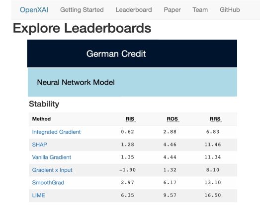
Figure 1: A snapshot of the leaderboard page from OpenXAI public website. We also provide interactive ranking functionality (arrow mark in the figure) which allows users to rank explanation methods based on metrics of their choice. Please visit the website to see leaderboards for other datasets.

3 Benchmarking Analysis

Next, we describe how we benchmark state-of-the-art explanation methods using our OpenXAI framework, and also discuss key findings of this benchmarking analysis. Code to reproduce all the results is available at https://github.com/AI4LIFE-GROUP/OpenXAI.

Experimental Setup. We benchmark all the six state-of-the-art feature attribution methods currently available in our OpenXAI framework along with the random baseline, using the openxai.Evaluator module (See Section 2). We use default hyperparameter settings for all these methods following the guidelines outlined in the original implementations. Details about the hyperparameters used in our experiments are discussed in Section  E.3 in the Appendix. Our OpenXAI framework currently has two pre-trained models, a logistic regression model and a deep neural network model, for each dataset. The neural network models have two fully connected hidden layers with 100 nodes in each layer, and they use ReLU activation functions and an output softmax layer. See Appendix E.4 for more details on model architectures, model training, and model performance.

Table 2: Ground-truth and predicted faithfulness results on the Heloc dataset for all explanation methods with LR model. Shown are average and standard error metric values computed across all instances in the test set. $\uparrow$ indicates that higher values are better, and $\downarrow$ indicates that lower values are better. Values corresponding to best performance are bolded.

Method	PRA ($\uparrow$)	RC ($\uparrow$)	FA ($\uparrow$)	RA ($\uparrow$)	SA ($\uparrow$)	SRA ($\uparrow$)	PGU ($\downarrow$)	PGI ($\uparrow$)
Random VanillaGrad IntegratedGrad Gradient x Input SmoothGrad SHAP LIME	0.500$\pm$0.00 1.0$\pm$0.00 1.0$\pm$0.00 0.641$\pm$0.00 1.0$\pm$0.00 0.645$\pm$0.00 0.982$\pm$0.00	0.005$\pm$0.01 1.0$\pm$0.00 1.0$\pm$0.00 0.390$\pm$0.01 1.0$\pm$0.00 0.384$\pm$0.01 0.994$\pm$0.00	0.498$\pm$0.00 0.957$\pm$0.00 0.957$\pm$0.00 0.582$\pm$0.00 0.957$\pm$0.00 0.586$\pm$0.00 0.932$\pm$0.00	0.043$\pm$0.00 0.957$\pm$0.00 0.957$\pm$0.00 0.049$\pm$0.00 0.957$\pm$0.00 0.054$\pm$0.00 0.671$\pm$0.00	0.251$\pm$0.00 0.469$\pm$0.01 0.469$\pm$0.01 0.255$\pm$0.01 0.274$\pm$0.00 0.269$\pm$0.01 0.929$\pm$0.00	0.022$\pm$0.00 0.469$\pm$0.01 0.469$\pm$0.01 0.022$\pm$0.00 0.274$\pm$0.00 0.024$\pm$0.00 0.670$\pm$0.00	0.033$\pm$0.00 0.034$\pm$0.00 0.034$\pm$0.00 0.033$\pm$0.00 0.015$\pm$0.00 0.033$\pm$0.00 0.042$\pm$0.00	0.035$\pm$0.00 0.036$\pm$0.00 0.036$\pm$0.00 0.036$\pm$0.00 0.047$\pm$0.00 0.036$\pm$0.00 0.029$\pm$0.001

Table 3: Ground-truth and predicted faithfulness results on the Adult Income dataset for all explanation methods with LR model. Shown are average and standard error metric values computed across all instances in the test set. $\uparrow$ indicates that higher values are better, and $\downarrow$ indicates that lower values are better. Values corresponding to best performance are bolded.

Method	PRA ($\uparrow$)	RC ($\uparrow$)	FA ($\uparrow$)	RA ($\uparrow$)	SA ($\uparrow$)	SRA ($\uparrow$)	PGU ($\downarrow$)	PGI ($\uparrow$)
Random VanillaGrad IntegratedGrad Gradient x Input SmoothGrad SHAP LIME	0.499$\pm$0.00 1.$\pm$0.00 1.$\pm$0.00 0.580$\pm$0.00 1.$\pm$0.00 0.655$\pm$0.00 0.913$\pm$0.00	0.0$\pm$0.00 1.$\pm$0.00 1.$\pm$0.00 0.281$\pm$0.00 1.$\pm$0.00 0.379$\pm$0.00 0.921$\pm$0.00	0.496$\pm$0.00 0.923$\pm$0.00 0.923$\pm$0.00 0.567$\pm$0.00 0.923$\pm$0.00 0.601$\pm$0.00 0.869$\pm$0.00	0.068$\pm$0.00 0.921$\pm$0.00 0.923$\pm$0.00 0.075$\pm$0.00 0.923$\pm$0.00 0.105$\pm$0.00 0.697$\pm$0.00	0.250$\pm$0.00 0.138$\pm$0.00 0.138$\pm$0.00 0.070$\pm$0.00 0.741$\pm$0.00 0.133$\pm$0.00 0.858$\pm$0.00	0.037$\pm$0.00 0.136$\pm$0.00 0.138$\pm$0.00 0.003$\pm$0.00 0.741$\pm$0.00 0.009$\pm$0.00 0.689$\pm$0.00	0.053$\pm$0.00 0.07$\pm$0.001 0.07$\pm$0.001 0.043$\pm$0.00 0.008$\pm$0.00 0.047$\pm$0.00 0.014$\pm$0.00	0.06$\pm$0.00 0.039$\pm$0.001 0.039$\pm$0.001 0.073$\pm$0.00 0.099$\pm$0.001 0.068$\pm$0.00 0.094$\pm$0.001

Faithfulness. We evaluate the ground-truth and predictive faithfulness of explanations generated by state-of-the-art methods using both synthetic and real-world datasets.

Ground-truth faithfulness: We evaluate ground-truth faithfulness by calculating the similarity between the generated explanations and the ground-truth explanations using the metrics discussed in Section 2. Results for various ground-truth faithfulness metrics are shown in Tables 2, 3, 16, 17. Vanilla Gradients, SmoothGrad, and Integrated Gradients produce explanations that achieve perfect scores on four ground-truth faithfulness metrics, viz. pairwise rank agreement (PRA), feature agreement (FA), rank agreement (RA), and rank correlation (RC) metrics, for all datasets. However, on average, across all datasets, LIME outperforms other methods on the signed agreement (SA) [+61.6%] and signed-rank agreement (SRA) [+65.3%] metrics, whereas gradient-based explainers achieve relatively lower values. While illustrative in nature, these findings show how OpenXAI can help identify the limitations of existing explanation methods, which in turn can inform the design of new methods.

Predictive faithfulness: Tables 2, 3, 16, 17 show results for the PGI and PGU metrics implemented in OpenXAI (see Section 2 and Appendix A). Overall, we find that SmoothGrad explanations are most faithful to the underlying model and, on average, across multiple datasets outperform other feature-attribution methods on PGU metric (+43.03%). However, results from the German credit dataset for the ANN model show that Gradient x Input produces considerably more faithful (+6.74%) explanations than other methods. Finally, this analysis confirms the finding by Krishna et al. [43] that explanations output by state-of-the-art methods do not necessarily align with each other. This finding further highlights the need for rigorous empirical and theoretical benchmarking of explanation methods.

Stability. Next, we examine the stability of explanation methods when the underlying models are LR models in Tables  3 and 3, and neural network models in Tables E.6 and E.6 in the Appendix. Due to space constraints, we focus on RIS and RRS metrics in the main paper and leave the other results to the Appendix. Overall, the relative stability varies considerably across different datasets, implying that no single explanation method is consistently the most stable. First, for the synthetic dataset in Table 3, we find that Gradient x Input, on average, outperforms feature-attribution methods in relative input stability (+93.5%, RIS) and relative representation stability (+59.2%, RRS). However, stability of Gradient x Input significantly degrades on real-world datasets (Table 3, E.6, E.6). Second, as shown in Tables 3, E.6, and E.6, there is no single explanation method that has the highest input and representation stability across all the real-world datasets. On average, across all real-world datasets, SmoothGrad achieves 63.2% higher RRS values compared to other methods, whereas no method performs consistently well when it comes to the RIS metric.

Table 4: Stability of explanation methods on the Synthetic dataset with LR model. Shown are average and standard error values across all test set instances. Values closer to zero are desirable, and the best performance is bolded.

Method	RIS	RRS
Random Vanilla Gradients Integrated Gradients Gradient x Input SmoothGrad SHAP LIME	6.868$\pm$0.013 6.133$\pm$0.011 5.957$\pm$0.013 0.405$\pm$0.015 5.249$\pm$0.008 5.673$\pm$0.012 9.355$\pm$0.008	6.687$\pm$0.015 6.144$\pm$0.006 9.022$\pm$0.043 3.422$\pm$0.037 9.419$\pm$0.037 8.751$\pm$0.035 13.564$\pm$0.036

Table 5: Stability of explanation methods on the German Credit dataset with LR model. Shown are average and standard error values across all test set instances. Values closer to zero are desirable, and the best performance is bolded.

Method	RIS	RRS
Random Vanilla Gradients Integrated Gradients Gradient x Input SmoothGrad SHAP LIME	6.274$\pm$0.104 -1.384$\pm$0.112 -2.004$\pm$0.119 -0.906$\pm$0.104 -4.780$\pm$0.117 -0.230$\pm$0.109 -0.698$\pm$0.109	16.448$\pm$0.124 5.241$\pm$0.024 4.560$\pm$0.029 9.437$\pm$0.124 4.931$\pm$0.122 10.056$\pm$0.115 9.397$\pm$0.119

Fairness. To measure fairness of explanation methods, we compute the average metric values (for each of the aforementioned faithfulness and stability metrics) for different subgroups (e.g., male and female) in the dataset and compare them. Larger gaps between the metric values for different subgroups indicates higher disparities (unfairness). Without loss of generality, we present results using the PGU (see Section 2 and Appendix A) metric. Results for LR models in Figures  2 and 3 provide two key findings. First, the fairness analysis in Figures  2 and 3 shows that there are disparities in the faithfulness of explanations (see Section 2) output by several methods (Vanilla Gradients, Integrated Gradients, and SmoothGrad). Second, Gradient x Input results in the least amount of disparity across both the datasets. These results also suggest a trade-off between various evaluation metrics. For instance, Gradient x Input method underperforms on faithfulness and stability metrics, but outperforms other methods (+8.9%) when it comes to fairness metrics. Given such trade-offs, practitioners can leverage the OpenXAI leaderboards (Figure 1) to select an explanation method that best meets application-specific needs. Results with NN models and other fairness metrics are included in the Appendix E.7.

Figure 2: Fairness analysis of PGU metric on the German Credit dataset with LR model. Shown are average and standard error values for majority (male) and minority (female) subgroups. Larger gaps between the values of majority and minority subgroups (i.e, red and blue bars respectively) indicate higher disparities which are undesirable.

Figure 3: Fairness analysis of PGU metric on the Adult Income dataset with LR model. Shown are average and standard error values for majority (male) and minority (female) subgroups. Larger gaps between the values of majority and minority subgroups (i.e, red and blue bars respectively) indicate higher disparities which are undesirable.

4 Conclusions

As post hoc explanations are increasingly being employed to aid decision makers and relevant stakeholders in various high-stakes applications, it becomes important to ensure that these explanations are reliable. To this end, we introduce OpenXAI, an open-source ecosystem comprising of XAI-ready datasets, implementations of state-of-the-art explanation methods, evaluation metrics, leaderboards and documentation to promote transparency and collaboration around evaluations of post hoc explanations. OpenXAI can readily be used to benchmark new explanation methods as well as incorporate them into our framework and leaderboards. By enabling systematic and efficient evaluation and benchmarking of existing and new explanation methods, OpenXAI can inform and accelerate new research in the emerging field of XAI. OpenXAI will be regularly updated with new datasets, explanation methods, and evaluation metrics, and welcomes input from the community.

Appendix A Evaluation Metrics

Here, we describe different evaluation metrics that we included in the first iteration of OpenXAI. More specifically, we discuss various metrics (and their implementations) for evaluating the faithfulness, stability, and fairness of explanations generated using a given feature attribution method.

1) Faithfulness. To measure how faithfully a given explanation mimics the underlying model, prior work has either leveraged synthetic datasets to obtain ground truth explanations or measured the differences in predictions when feature values are perturbed [59]. Here, we discuss the two broad categories of faithfulness metrics included in OpenXAI, namely ground-truth and predictive faithfulness.

a) Ground-truth Faithfulness. OpenXAI leverages the following metrics outlined by Krishna et al. [43] to calculate the agreement between ground-truth explanations (i.e., coefficients of logistic regression models) and explanations generated by state-of-the-art methods.

• Feature Agreement (FA) metric computes the fraction of top-$K$ features that are common between a given post hoc explanation and the corresponding ground truth explanation.

• Rank Agreement (RA) metric measures the fraction of top-$K$ features that are not only common between a given post hoc explanation and the corresponding ground truth explanation, but also have the same position in the respective rank orders.

• Sign Agreement (SA) metric computes the fraction of top-$K$ features that are not only common between a given post hoc explanation and the corresponding ground truth explanation, but also share the same sign (direction of contribution) in both the explanations.

• Signed Rank Agreement (SRA) metric computes the fraction of top-$K$ features that are not only common between a given post hoc explanation and the corresponding ground truth explanation, but also share the same feature attribution sign (direction of contribution) and position (rank) in both the explanations.

• Rank Correlation (RC) metric computes the Spearman’s rank correlation coefficient to measure the agreement between feature rankings provided by a given post hoc explanation and the corresponding ground truth explanation.

• Pairwise Rank Agreement (PRA) metric captures if the relative ordering of every pair of features is the same for a given post hoc explanation as well as the corresponding ground truth explanation i.e., if feature A is more important than B according to one explanation, then the same should be true for the other explanation. More specifically, this metric computes the fraction of feature pairs for which the relative ordering is the same between the two explanations.

Reported metric values. While the aforementioned metrics quantify the ground-truth faithfulness of individual explanations, we report a single value corresponding to each explanation method and dataset to facilitate easy comparison of state-of-the-art methods. To this end, we adopt a similar strategy as that of Krishna et al. [43] and compute the aforementioned metrics for each instance in the test data and then average these values. To arrive at the reported values of FA, RA, SA, and SRA metrics, instead of setting a specific value for $K$, we do the above computation for all possible values of $K$ and then plot the different values of $K$ (on the x-axis) and the corresponding averaged metric values (on the y-axis), and calculate the area under the resulting curve (AUC). On the other hand, in case of RC and PRA metrics, we set $K$ to the total number of features and compute the averaged metric values (across all test instances) as discussed above.

b) Predictive Faithfulness. Following Petsiuk et al. [59], OpenXAI includes two complementary predictive faithfulness metrics: i) Prediction Gap on Important feature perturbation (PGI) which measures the difference in prediction probability that results from perturbing the features deemed as influential by a given post hoc explanation, and ii) Prediction Gap on Unimportant feature perturbation (PGU) which measures the difference in prediction probability that results from perturbing the features deemed as unimportant by a given post hoc explanation.

For a given instance $\mathbf{x}$, we first obtain the prediction probability $\hat{y}$ output by the underlying model $f$, i.e., $\hat{y}=f(\mathbf{x})$. Let $e_{\mathbf{x}}$ be an explanation for the model prediction of $\mathbf{x}$. In case of PGU, we then generate a perturbed instance $\mathbf{x}^{\prime}$ in the local neighborhood of $\mathbf{x}$ by holding the top-$k$ features constant, and slightly perturbing the values of all the other features by adding a small amount of Gaussian noise. In case of PGI, we generate a perturbed instance $\mathbf{x}^{\prime}$ in the local neighborhood of $\mathbf{x}$ by slightly perturbing the values of the top-$k$ features by adding a small amount of Gaussian noise, and holding all the other features constant. Finally, we compute the expected value of the prediction difference between the original and perturbed instances as:

$$\textup{PGI}(\mathbf{x},f,e_{\mathbf{x}},k)=\mathbb{E}_{\mathbf{x}^{\prime}\sim\textnormal{perturb($\mathbf{x}$, $e_{\mathbf{x}}$, top-$K$)}}[|\hat{y}-f(\mathbf{x}^{\prime})|],$$ (1)

$$\textup{PGU}(\mathbf{x},f,e_{\mathbf{x}},k)=\mathbb{E}_{\mathbf{x}^{\prime}\sim\textnormal{perturb($\mathbf{x}$, $e_{\mathbf{x}}$, non top-$K$)}}[|\hat{y}-f(\mathbf{x}^{\prime})|],$$ (2)

where perturb($\cdot$) returns the noisy versions of $\mathbf{x}$ as described above.

Reported metric values. Similar to the ground-truth faithfulness metrics, we report PGI and PGU by calculating the AUC over all values of $K$.

2) Stability. We leverage the metrics Relative Input Stability (RIS), Relative Representation Stability (RRS), and Relative Output Stability (ROS) [4] which measure the maximum change in explanation relative to changes in the inputs, internal representations learned by the model, and output prediction probabilities respectively. These metrics can be written formally as:

$$\textup{RIS}(\mathbf{x},\mathbf{x}^{\prime},\mathbf{e}_{\mathbf{x}},\mathbf{e}_{\mathbf{x}^{\prime}})=\max_{\mathbf{x}^{\prime}}\frac{||\frac{(\mathbf{e}_{\mathbf{x}}-\mathbf{e}_{\mathbf{x}^{\prime}})}{\mathbf{e}_{\mathbf{x}}}||_{p}}{\max(||\frac{(\mathbf{x}-\mathbf{x}^{\prime})}{\mathbf{x}}||_{p},\epsilon_{min})},\leavevmode\nobreak\ \forall\mathbf{x}^{\prime}\leavevmode\nobreak\ \textup{s.t.}\leavevmode\nobreak\ \mathbf{x}^{\prime}\in\mathcal{N}_{\mathbf{x}};\leavevmode\nobreak\ \hat{y}_{\mathbf{x}}=\hat{y}_{\mathbf{x}^{\prime}}$$ (3)

where $\mathcal{N}_{\mathbf{x}}$ is a neighborhood of instances $\mathbf{x}^{\prime}$ around $\mathbf{x}$, and $\mathbf{e}_{\mathbf{x}}$ and $\mathbf{e}_{\mathbf{x^{\prime}}}$ denote the explanations corresponding to instances $\mathbf{x}$ and $\mathbf{x}^{\prime}$, respectively. The numerator of the metric measures the $l_{p}$ norm of the percent change of explanation $\mathbf{e}_{\mathbf{x}^{\prime}}$ on the perturbed instance $\mathbf{x}^{\prime}$ with respect to the explanation $\mathbf{e}_{\mathbf{x}}$ on the original point $\mathbf{x}$. The denominator measures the $l_{p}$ norm between the (normalized) inputs $\mathbf{x}$ and $\mathbf{x}^{\prime}$, and the max term in the denominator prevents division by zero.

$$\textup{RRS}(\mathbf{x},\mathbf{x}^{\prime},\mathbf{e}_{\mathbf{x}},\mathbf{e}_{\mathbf{x}^{\prime}})=\max_{\mathbf{x}^{\prime}}\frac{||\frac{(\mathbf{e}_{\mathbf{x}}-\mathbf{e}_{\mathbf{x}^{\prime}})}{\mathbf{e}_{\mathbf{x}}}||_{p}}{\max(||\frac{(\mathcal{L}_{\mathbf{x}}{-}\mathcal{L}_{\mathbf{x}^{\prime}})}{\mathcal{L}_{\mathbf{x}}}||_{p},\epsilon_{min})},\leavevmode\nobreak\ \forall\mathbf{x}^{\prime}\leavevmode\nobreak\ \leavevmode\nobreak\ \textup{s.t.}\leavevmode\nobreak\ \leavevmode\nobreak\ \mathbf{x}^{\prime}\in\mathcal{N}_{\mathbf{x}};\leavevmode\nobreak\ \leavevmode\nobreak\ \hat{y}_{\mathbf{x}}{=}\hat{y}_{\mathbf{x}^{\prime}}$$ (4)

where $\mathcal{L}(\cdot)$ denotes the internal representations learned by the model. Without loss of generality, we use a two layer neural network model in our experiments and use the output of the first layer for computing RRS. Similarly, we can also define ROS as:

$$\textup{ROS}(\mathbf{x},\mathbf{x}^{\prime},\mathbf{e}_{\mathbf{x}},\mathbf{e}_{\mathbf{x}^{\prime}})=\max_{\mathbf{x}^{\prime}}\frac{||\frac{(\mathbf{e}_{\mathbf{x}}-\mathbf{e}_{\mathbf{x}^{\prime}})}{\mathbf{e}_{\mathbf{x}}}||_{p}}{\max(||\frac{(f({\mathbf{x}}){-}f({\mathbf{x}^{\prime}})}{f({\mathbf{x}})}||_{p},\epsilon_{min})},\leavevmode\nobreak\ \forall\mathbf{x}^{\prime}\leavevmode\nobreak\ \leavevmode\nobreak\ \textup{s.t.}\leavevmode\nobreak\ \leavevmode\nobreak\ \mathbf{x}^{\prime}\in\mathcal{N}_{\mathbf{x}};\leavevmode\nobreak\ \leavevmode\nobreak\ \hat{y}_{\mathbf{x}}{=}\hat{y}_{\mathbf{x}^{\prime}},$$ (5)

where $f(\mathbf{x})$ and $f(\mathbf{x}^{\prime})$ are the output prediction probabilities for $\mathbf{x}$ and $\mathbf{x}^{\prime}$, respectively. To the best of our knowledge, OpenXAI is the first benchmark to incorporate all the above stability metrics.

Reported metric values.. We compute the aforementioned metrics for each instance in the test set, and then average these values.

3) Fairness. It is important to ensure that there are no significant disparities between the reliability of post hoc explanations corresponding to instances in the majority and the minority subgroups. To this end, we average all the aforementioned metric values across instances in the majority and minority subgroups, and then compare the two estimates (See Figures 3, 2, 5 etc.) to check if there are significant disparities [18].

Appendix B Additional Related Work

Our work builds on the vast literature on model interpretability and explainability. Below is an overview of additional works that were not included in Section 1 due to space constraints.

Inherently Interpretable Models and Post hoc Explanations. Many approaches learn inherently interpretable models such as rule lists [80, 77], decision trees and decision lists [48], and others [46, 13, 53, 15]. However, complex models such as deep neural networks often achieve higher accuracy than simpler models [62]. Thus, there has been significant interest in constructing post hoc explanations to understand their behavior. To this end, several techniques have been proposed in recent literature to construct post hoc explanations of complex decision models. For instance, LIME, SHAP, Anchors, BayesLIME, and BayesSHAP [62, 55, 63, 69] are considered perturbation-based local explanation methods because they leverage perturbations of individual instances to construct interpretable local approximations (e.g., linear models). On the other hand, methods such as Vanilla Gradients, Gradient x Input, SmoothGrad, Integrated Gradients, and GradCAM [67, 72, 65, 70] are referred to as gradient-based local explanation methods since they leverage gradients computed with respect to input features of individual instances to explain individual model predictions.

There has also been recent work on constructing counterfactual explanations which capture what changes need to be made to a given instance in order to flip its prediction [76, 74, 37, 61, 52, 11, 38, 57, 39, 58]. Such explanations can be leveraged to provide recourse to individuals negatively impacted by algorithmic decisions. An alternate class of methods referred to as global explanation methods attempt to summarize the behavior of black-box models as a whole rather than in relation to individual data points [47, 12]. A more detailed treatment of this topic is provided in other comprehensive survey articles [8, 30, 56, 49, 17].

In this work, we focus primarily on local feature attribution-based post hoc explanation methods i.e., explanation methods which attempt to explain individual model predictions by outputting a vector of feature importances. More specifically, the goal of this work is to enable systematic benchmarking of these methods in an efficient and transparent manner.

Evaluating Post hoc Explanations. In addition to the quantitative metrics designed to evaluate the reliability of post hoc explanation methods [51, 81, 7, 18] (See Section 1), prior works have also introduced human-grounded approaches to evaluate the interpretability of explanations generated by these methods [21]. For example, Lakkaraju and Bastani [45] carry out a user study to understand if misleading explanations can fool domain experts into deploying racially biased models, while Kaur et al. [40] find that explanations are often over-trusted and misused. Similarly, Poursabzi-Sangdeh et al. [60] find that supposedly-interpretable models can lead to a decreased ability to detect and correct model mistakes, possibly due to information overload. Jesus et al. [35] introduce a method to compare explanation methods based on how subject matter experts perform on specific tasks with the help of explanations. Lage et al. [44] use insights from rigorous human-subject experiments to inform regularizers used in explanation algorithms. In contrast to the aforementioned research, our work leverages twenty-two different state-of-the-art quantitative metrics to systematically benchmark the reliability (and not interpretability) of post hoc explanation methods.

Limitations and Vulnerabilities of Post hoc Explanations. Various quantitative metrics proposed in literature (See Section 1) were also leveraged to analyze the behavior of post hoc explanation methods and their vulnerabilities—e.g., Ghorbani et al. [29] and Slack et al. [68] demonstrated that methods such as LIME and SHAP may result in explanations that are not only inconsistent and unstable, but also prone to adversarial attacks. Furthermore Lakkaraju and Bastani [45] and Slack et al. [68] showed that explanations which do not accurately represent the importance of sensitive attributes (e.g., race, gender) could potentially mislead end users into believing that the underlying models are fair when they are not [45, 68, 6]. This, in turn, could lead to the deployment of unfair models in critical real world applications. There is also some discussion about whether models which are not inherently interpretable ought to be used in high-stakes decisions at all. Rudin [64] argues that post hoc explanations tend to be unfaithful to the model to the extent that their usefulness is severely compromised. While this line of work demonstrates different ways in which explanations could potentially induce inaccuracies and biases in real world applications, they do not focus on systematic benchmarking of post hoc explanation methods which is the main goal of our work.

Appendix C Synthetic Dataset

Our proposed data generation process described in Algorithm 1 is designed to encapsulate arbitrary feature dependencies, unambiguous definitions of local neighborhoods, and clear descriptions of feature influences. In our algorithm 1, the local neighborhood of a sample is controlled by its cluster membership $k$, while the degree of feature dependency can be easily controlled by the user setting $\Sigma_{k}$ to desired values. The default value of $\Sigma_{k}=\mathbf{I}$, where $\mathbf{I}$ is the identity matrix, indicating that all features are independent of one another. The elements of the true underlying weight vector $w_{k}$ are sampled from a uniform distribution: $w_{k}\sim\mathcal{U}(l,u)$. We set $l=-1$ and $u=1$. The masking vectors $m_{k}$ with elements $m_{k,j}$ are generated by a Bernoulli distribution: $m_{k,j}\sim\mathcal{B}(p)$, where the parameter $p$ controls the ground-truth explanation sparsity. We set $p=0.25$. Further, the cluster centers are chosen as follows: when the number of features $d$ is smaller than or equal to the number of clusters $K$, then we set the first cluster center to $[1,0,\dots,0]$, the second one to $[0,1,\dots,0]$, etc. We also introduce a multiplier $\kappa$ to control the distance between the cluster centers so that the cluster centers are located at $\mu_{1}=\kappa\cdot[1,0,\dots,0]$, $\mu_{2}=\kappa\cdot[0,1,\dots,0]$, etc. We set $\kappa=6$. In general, we have observed that lower values of $\kappa$ result in more complex classification problems. When the number of features $d$ is greater than the number of clusters $K$, we adjust the above described approach slightly: we first compute $\ell=\lfloor K/d\rfloor$, and then we compute the cluster centers for the first $d$ clusters as described above, for the next $d$ clusters we use $\mu_{d+1}=2\kappa\cdot[1,0,\dots,0]$, $\mu_{d+2}=2\kappa\cdot[0,1,\dots,0]$, etc. If $\ell=1$, we stop this procedure here, else we continue, and repeat filling up the clusters $\mu_{2d+1}=3\kappa\cdot[1,0,\dots,0]$, $\mu_{2d+2}=3\kappa\cdot[0,1,\dots,0]$, etc.

input :  number of clusters: $K$, cluster centers: $[\mu_{1},\mu_{2},\dots,\mu_{K}]$, cluster variances: $[\Sigma_{1},\dots,\Sigma_{K}]$, Weight vectors: $[w_{1},\dots,w_{K}]$, masking vectors: $[m_{1},\dots,m_{K}]$

output :  features: $\mathbf{X}$, labels: $\mathbf{y}$

$\mathbf{X}=\mathbf{0}_{n\times d}$ ;

$\Pi=\mathbf{0}_{n\times 1}$ ;

for $i=1$:$n$ do

       $k\leftarrow$ Cat($K$)    # Randomly picks a cluster index ;

       $x_{i}\sim\mathcal{N}(\mu_{k},\Sigma_{k})$    # Samples Gaussian instance ;

       $\mathbf{X}[i,:]=x_{i}$ ;

       $\pi_{1}=\mathbb{P}(y_{i}=1|\mathbf{x}_{i})=\frac{\exp\big{(}(w_{k}\odot m_{k})^{\top}x_{i}\big{)}}{1+\exp\big{(}(w_{k}\odot m_{k})^{\top}x_{i}\big{)}}$    # Get class probability ;

       $\Pi[i]=\pi_{1}$ ;

      

$\tilde{\pi}=\texttt{get\_median}(\Pi)$ ;

for $i=1$:$n$ do

       $y_{i}=\mathbb{I}(\Pi[i]>\tilde{\pi})$     # Make sure classes are balanced ;

      

Return: $\mathbf{X},\mathbf{y}$ ;

Algorithm 1 SynthGauss

Theorem 1

If a given dataset encapsulates the properties of feature independence, unambiguous and well-separated local neighborhoods, and a unique ground truth explanation for each local neighborhood, the most accurate model trained on such a dataset will adhere to the unique ground truth explanation of each local neighborhood.

Proof: Before we describe the proof, we begin by first formalizing the properties of feature independence, unambiguous and well-separated local neighborhoods, and a unique ground truth explanation for each local neighborhood using some notation. Let $A=[a_{1},a_{2},\cdots a_{d}]$ denote the vector of input features in a given dataset $D$, and let the instances in the dataset $D$ be separated into $K$ clusters (local neighborhoods) based on their proximity.

Feature independence: The dataset $D$ satisfies feature independence if $P(a_{i}|a_{j})=P(a_{i})$ $\forall i,j\in\{1,2,\cdots d\}$ and $i\neq j$.

Unambiguous and well-separated local neighborhoods: The dataset $D$ is said to constitute unambiguous and well-separated local neighborhoods if $dist(x_{i,j},x_{p,q})\gg dist(x_{i,j},x_{i,l})$ $\forall i,p\in\{1,2\cdots K\}$ where $x_{i,j}$ and $x_{i,l}$ are the $j^{th}$ and $l^{th}$ instances of some cluster $i$, $x_{p,q}$ is the $q^{th}$ instance of cluster $p$ and $p\neq i$. The above implies that the distances between points in different clusters should be significantly higher than the distances between points in the same cluster.

Unique ground truth explanation for each local neighborhood: The dataset $D$ is said to comprise of unique ground truth explanations for each local neighborhood if the ground truth labels of instances in each cluster $k\in\{1,2\cdots K\}$ are generated as a function of a subset of features $A_{k}\subseteq A$ where there is a clear relative ordering among features in $A_{k}$ which is captured by the weight vector $w_{k}$, and features in $A$ are completely independent of each other. [Note that the influential feature set $A_{k}$ corresponding to the cluster $k$ is also captured using the mask vector $m_{k}$ (See Section 2) where $m_{k,i}=1$ if the $i^{th}$ feature is in set $A_{k}$]. This would imply that there is a clear description of the top-$T$ features (and their relative ordering) where $T\leq|A_{k}|$ influence the ground truth labeling process.

With the above information in place, let us now consider a model $\mathcal{M}$ which is trained on the dataset $D$ and achieves highest possible accuracy on it. To show that this model indeed adheres to the unique ground truth explanations of each of the local neighborhoods (clusters), we adopt the strategy of proof by contradiction. To this end, we begin with the assumption that the model $\mathcal{M}$ does not adhere to the unique ground truth explanation of some local neighborhood $k\in\{1,2,\cdots K\}$ i.e., the top-$T$ features leveraged by model $\mathcal{M}$ for instances in cluster $k$ (denoted by $\mathcal{M}^{k}_{T}$) do not exactly match the top-$T$ features leveraged by the ground truth labeling process where $T\leq|A_{k}|$. This happens either when there is a mismatch in the relative ordering among the top-$T$ features used by the model $\mathcal{M}$ and the ground truth labeling process (or) when there is at least one feature $a$ that appears among the top-$T$ features used by the model but not the ground truth labeling process. In either case, we can construct another model $\mathcal{M}^{\prime}$ such that the top-$T$ features used by $\mathcal{M}^{\prime}$ match the top-$T$ features of the ground truth labeling process exactly, and the accuracy of $\mathcal{M}^{\prime}$ will be higher than that of $\mathcal{M}$. This contradicts the assumption that the model $\mathcal{M}$ has the highest possible accuracy, thus demonstrating that the model with highest possible accuracy would adhere to the unique ground truth explanation of each local neighborhood.

Appendix D Extending OpenXAI

Figure 4: A snapshot of the OpenXAI leaderboard submission form. Users can use this single form to incorporate new datasets, pre-trained models, explanation methods, and evaluation metrics into OpenXAI framework.

In this section, we walk through how users can extend and contribute to OpenXAI by adding custom datasets, pre-trained models, explanation methods, or evaluation metrics. In Figure 4, we show a snapshot of our FORM that can be used by users to submit requests for new datasets, pre-trained models, explanation methods, or evaluation metrics.

Custom Datasets. Adding new datasets into OpenXAI ’s pipeline is as simple as uploading a .csv file or a .zip folder. Users can submit requests to incorporate new datasets into OpenXAI by providing either the complete dataset (with or without data splits) or individual training and testing files for the respective dataset.

Custom Predictive Models. Users can also submit requests to include new pre-trained models into the OpenXAI framework. Here, users have to provide i) model architecture and implementation details, ii) model hyperparameters and training details, and iii) trained weights for reproducing model performance.

Custom Evaluation Metrics. Users can include new evaluation metrics into OpenXAI by filling out the submit request form and providing the GitHub link to their code and a summary of their metrics. Once approved, the metric should be implemented as a function in the Evaluator class. The input data, ground-truth labels, model predictions, explanations, and the underlying black-box model are all provided in the Evaluator class. The evaluation metric should return a scalar score as a part of their respective implementation.

Custom Explanation Methods. Users can include new explanation methods into OpenXAI ’s list of explainers by following the openxai.Explainer template. The abstract method defined ensures that the output of new/existing explanation methods returns explanations as a tensor. Note that all custom explanation methods should extend the Explainer class. Finally, users must provide the GitHub link to their code and a summary of their explanation method.

We invite submissions to any one or multiple benchmarks in OpenXAI. To be included in the leaderboard, please fill out this FORM, include results of your explanation method and provide the full implementation of your algorithm with proper documentations and GitHub link.

Appendix E Benchmarking Analysis

E.1 Real-World Datasets

In addition to synthetic dataset, OpenXAI library includes five real-world benchmark datasets from high-stakes domains. Table 1 provides a summary of the real-world datasets currently included in OpenXAI. Our library implements multiple data split strategies and allows users to customize the percentages of train-test splits. To this end, if a given dataset comes with a pre-determined train and test splits, OpenXAI loads the training and testing dataloaders from those pre-determined splits. Otherwise, OpenXAI’s dataloader divides the entire dataset randomly into train (70%) and test (30%). Next, we detail the covariates $\mathbf{x}$ and labels $\mathbf{y}$ for each dataset.

German Credit. The dataset comprises of demographic (age, gender), personal (marital status), and financial (income, credit duration) features from 1,000 credit applicants, where they are categorized into good vs. bad customer depending on their credit risk [22].

COMPAS. The dataset has criminal records and demographics features for 18,876 defendants who got released on bail at the U.S state courts during 1990-2009. The task is to classify defendants into bail (i.e., unlikely to commit a violent crime if released) vs. no bail (i.e., likely to commit a violent crime) [36].

Adult Income. The dataset contains demographic (e.g., age, race, and gender), education (degree), employment (occupation, hours-per week), personal (marital status, relationship), and financial (capital gain/loss) features for 48,842 individuals. The task is to predict whether an individual’s income exceeds $50K per year vs. not [79].

Give Me Some Credit. The dataset incorporates demographic (age), personal (number of dependents), and financial (e.g., monthly income, debt ratio, etc.) features for 250,000 individuals. The task is to predict the probability that a customer will experience financial distress vs. not in the next two years. The aim of the dataset is to build models that customers can use to the best financial decisions [27].

Home Equity Line of Credit (HELOC). The dataset comprises of financial (e.g., total number of trades, average credit months in file) attributes from anonymized applications submitted by 9,871 real homeowners. A HELOC is a line of credit typically offered by a bank as a percentage of home equity. The fundamental task is to use the information about the applicant in their credit report to predict whether they will repay their HELOC account within 2 years [25].

E.2 Explanation Methods

OpenXAI provides implementations for six explanation methods: Vanilla Gradients [67], Integrated Gradients [72], SmoothGrad [70], Gradient x Input [66], LIME [62], and SHAP [55]. Table E.2 summarizes how these methods differ along two axes: whether each method requires “White-box Access” to model gradients and whether each method learns a local approximation model to generate explanations.

Table 6: Summary of currently available feature attribution methods in OpenXAI. “Learning?” denotes whether learning/training procedures are required to generate explanations and "White-box Access?" denotes if the access to the internals of the model (e.g., gradients) are needed.

Method	Learning?	White-box Access?
Random VanillaGrad IntegratedGrad Gradient x Input SmoothGrad SHAP LIME	✗ ✗ ✗ ✗ ✗ ✓ ✓	✗ ✓ ✓ ✓ ✓ ✗ ✗

Implementations. We used existing public implementations of all explanation methods in our experiments. We used the following captum software package classes: i) captum.attr.Saliency for Vanilla Gradients; ii) captum.attr.IntegratedGradients for Integrated Gradients; iii) captum.attr.NoiseTunnel and captum.attr.Saliency for SmoothGrad; iv) captum.attr.InputXGradient for Gradient x Input; and v) captum.attr.KernelShap for SHAP. Finally, we use the authors’ LIME python package for LIME.

E.3 Hyperparameter details

OpenXAI uses default hyperparameter settings for all explanation methods following the authors’ guidelines. Every explanation method has a corresponding parameter dictionary that stores all the default parameter values. Below, we detail the hyperparameters of individual explanation methods used in our experiments.

a) params_lime = {‘lime_mode’: ‘tabular’, ‘lime_sample_around_instance’: True, ‘lime_kernel_ width’: 0.75, ‘lime_n_samples’: 1000, ‘lime_discretize_continuous’: False, ‘lime_standard_ deviation’: float(np.sqrt(0.05))}

Description. The option ‘tabular’ indicates that we wish to compute explanations on a tabular data set. The option ‘lime_sample_around_instance’ makes sure that the sampling is conducted in a local neighborhood around the point that we wish to explain. The ‘lime_discretize_continuous’ option ensures that continuous variables are kept continuous, and are not discretized. This parameter sets the ‘lime_standard_ deviation’ of the Gaussian random variable that is used to sample around the instance that we wish to explain. We set this to a small value, ensuring that we in fact sample from a local neighborhood.

b) params_shap = {‘shap_subset_size’: 50, ‘perturbations_per_eval’: 1, ‘feature_mask’: None, ‘baselines’: None}

Description. The parameter ‘shap_subset_size’ controls the number of samples of the original model used to train the surrogate SHAP model, ‘perturbations_per_eval’ allows the processing of multiple samples simultaneously, ‘feature_mask’ defines a mask on the input instance that group features corresponding to the same interpretable feature, and ‘baselines’ defines the reference value which replaces each feature when the corresponding interpretable feature is set to 0.

c) params_grads = {‘grad_absolute_value’: False}

Description. The parameter ‘grad_absolute_value’ controls whether the absolute value of each element in the explanation vector should be taken or not.

d) params_sg = {‘sg_n_samples’: 500, ‘sg_standard_deviation’: float(np.sqrt(0.05))}

Description. The parameter ‘sg_n_samples’ sets the number of samples used in the Gaussian random variable to smooth the gradient, while ‘sg_standard_deviation’ determines the size of the local neighboorhood the gaussian random variables are sampled from. We use a small value, ensuring that we in fact sample from a local neighborhood.

e) params_ig = {‘ig_method’: ‘gausslegendre’, ‘ig_multiply_by_inputs’: False, ‘ig_baseline’: ‘mean’}

Further, we parameterized our data generating process as follows.

f) params_gauss = {‘n_samples’: 1000, ‘dim’:20, ‘n_clusters’: 10, ‘distance_to_center’: 6, ‘test_size’: 0.25, ‘upper_weight’: 1, ‘lower_weight’: -1, ‘seed’: 564, ‘sigma’: None, ‘sparsity’: 0.25}

Description. The above parameters can be matched with the parameters from the data generating process described in Appendix C: in particular, ‘sparsity’$=p$, ‘upper_weight’ $=u$, ‘lower_weight’ $=l$, ‘dim’$=d$, ‘n_clusters’ $=K$, ‘distance_to_center’ $=\kappa$ and ‘sigma’=None implies that the identity matrix is used, i.e., $\Sigma_{k}=\mathbf{I}$.

In addition, for a given instance $\mathbf{x}$, some evaluation metrics leverage a perturbation class to generate perturbed samples $\mathbf{x}^{\prime}$. We have a parameterized version of this perturbation class in OpenXAI with the following default parameters:

g) params_perturb = {‘perturbation_mean’ : 0.0, ‘perturbation_std’ : 0.05, ‘perturbation_ flip_percentage’ : 0.03}

Finally, we denote the top-$k$ value using {‘percentage_most_important’: 0.25}, i.e., we consistently use 25% of the top features for calculating our metric scores.

E.4 Model details

Our current release of OpenXAI has two pre-trained models: i) a logistic regression model and ii) a deep neural network model for all datasets. To support systematic, reproducible, and efficient benchmarking of post hoc explanation methods, we provide the model weights for both models trained on all six datasets in our pipeline. For neural network models, we use two fully connected hidden layers with 100 nodes in each layer, with ReLU activation functions and an output softmax layer for all datasets. We train both models for 50 epochs using an Adam optimizer with a learning rate of $\eta{=}0.001$. Next, we show the model performance of both models on all six datasets.

Table 7: Results of the machine learning models trained on six datasets. Shown are the accuracy of LR and ANN models trained the datasets. The best performance is bolded.

Dataset	LR	ANN
Synthetic Data German Credit HELOC COMPAS Adult Income Give Me Some Credit Framingham Heart Study Pima-Indians Diabetes	83.0% 72.0% 72.0% 85.4% 84.0% 94.1% 85.0% 66.0%	92.0% 75.0% 74.0% 85.0% 85.0% 95.0% 85.0% 77.0%

E.5 Additional results

The datasets included in our OpenXAI framework are diverse i.e., these datasets span a wide variety of sizes (ranging from 1000 instances to 102,209 instances in the dataset), feature dimensions (ranging from 7 to 23 dimensions), class imbalance ratios, and feature types (comprising a mix of continuous and discrete features). In addition, the datasets that we chose span two different real-world domains namely criminal justice, and lending. In addition, the datasets included in our OpenXAI framework are very popular and are widely employed in XAI and fairness research. For instance, several recent works in XAI have employed these datasets to both evaluate the efficacy of newly proposed methods as well as to study the behavior of existing methods. Furthermore, several of the datasets that we chose also include sensitive attributes which help us evaluate the (un)fairness (disparities) in explanation quality across majority and minority subgroups.

In response to the reviewer’s comment about the lack of diversity in the domains we consider, we included two new datasets from the healthcare domain and benchmarked state-of-the-art explanation methods on these datasets as well. More specifically, we included the Pima-Indians Diabetes [71] and Framingham heart study [1] datasets both of which have been utilized in recent XAI research. New results with these datasets are included in Section E.5 in the Appendix. We observe similar insights with these new datasets as well. We find that explanations constructed by SmoothGrad are on average more faithful (see Tables  8-11 in Appendix) and outperform other feature-attribution methods on the Prediction Gap on Unimportant feature perturbation (PGU) metric. The stability results of various explanation methods for logistic regression and neural network models are shown in Tables 8-9 and Tables 10,11 respectively in the Appendix. For logistic regression models, we do not find consistent trends across both the new datasets. On the other hand, in the case of neural network models, we observe that SmoothGrad, on average, outperforms other feature attribution methods on relative representation stability (RRS) and output stability (ROS) metrics.

Table 8: Ground-truth and predicted faithfulness results on the Pima Indians Diabetes dataset for all explanation methods with LR model. Shown are average and standard error metric values computed across all instances in the test set. $\uparrow$ indicates that higher values are better, and $\downarrow$ indicates that lower values are better. Values corresponding to best performance are bolded.

Method	PRA ($\uparrow$)	RC ($\uparrow$)	FA ($\uparrow$)	RA ($\uparrow$)	SA ($\uparrow$)	SRA ($\uparrow$)	PGU ($\downarrow$)	PGI ($\uparrow$)
Random VanillaGrad IntegratedGrad Gradient x Input SmoothGrad SHAP LIME	0.497$\pm$0.01 1.0$\pm$0.00 1.0$\pm$0.00 0.527$\pm$0.01 1.0$\pm$0.00 0.518$\pm$0.01 1.0$\pm$0.00	-0.047$\pm$0.03 1.0$\pm$0.00 1.0$\pm$0.00 0.043$\pm$0.02 1.0$\pm$0.00 0.048$\pm$0.02 1.0$\pm$0.00	0.486$\pm$0.00 0.875$\pm$0.00 0.875$\pm$0.00 0.477$\pm$0.01 0.875$\pm$0.00 0.479$\pm$0.01 0.874$\pm$0.01	0.111$\pm$0.00 0.875$\pm$0.00 0.875$\pm$0.00 0.066$\pm$0.01 0.875$\pm$0.00 0.064$\pm$0.01 0.874$\pm$0.00	0.239$\pm$0.00 0.131$\pm$0.02 0.131$\pm$0.02 0.082$\pm$0.02 0.731$\pm$0.00 0.090$\pm$0.02 0.875$\pm$0.00	0.054$\pm$0.00 0.131$\pm$0.03 0.131$\pm$0.03 0.017$\pm$0.00 0.731$\pm$0.00 0.016$\pm$0.00 0.873$\pm$0.00	0.011$\pm$0.00 0.013$\pm$0.00 0.013$\pm$0.00 0.011$\pm$0.00 0.008$\pm$0.00 0.011$\pm$0.00 0.01$\pm$0.00	0.013$\pm$0.00 0.012$\pm$0.00 0.012$\pm$0.00 0.014$\pm$0.00 0.016$\pm$0.00 0.014$\pm$0.00 0.015$\pm$0.001

Table 9: Ground-truth and predicted faithfulness results on the Framingham heart study dataset for all explanation methods with LR model. Shown are average and standard error metric values computed across all instances in the test set. $\uparrow$ indicates that higher values are better, and $\downarrow$ indicates that lower values are better. Values corresponding to best performance are bolded.

Method	PRA ($\uparrow$)	RC ($\uparrow$)	FA ($\uparrow$)	RA ($\uparrow$)	SA ($\uparrow$)	SRA ($\uparrow$)	PGU ($\downarrow$)	PGI ($\uparrow$)
Random VanillaGrad IntegratedGrad Gradient x Input SmoothGrad SHAP LIME	0.503$\pm$0.00 1.0$\pm$0.00 1.0$\pm$0.00 0.665$\pm$0.00 1.0$\pm$0.00 0.636$\pm$0.00 0.990$\pm$0.00	-0.001$\pm$0.01 1.0$\pm$0.00 1.0$\pm$0.00 0.463$\pm$0.00 1.0$\pm$0.00 0.384$\pm$0.00 0.995$\pm$0.00	0.498$\pm$0.00 0.933$\pm$0.00 0.933$\pm$0.00 0.651$\pm$0.00 0.933$\pm$0.00 0.657$\pm$0.00 0.925$\pm$0.00	0.062$\pm$0.00 0.933$\pm$0.00 0.933$\pm$0.00 0.243$\pm$0.01 0.933$\pm$0.00 0.241$\pm$0.00 0.866$\pm$0.00	0.250$\pm$0.00 0.022$\pm$0.00 0.022$\pm$0.00 0.015$\pm$0.00 0.724$\pm$0.00 0.052$\pm$0.00 0.925$\pm$0.00	0.032$\pm$0.00 0.022$\pm$0.00 0.022$\pm$0.00 0.007$\pm$0.00 0.724$\pm$0.00 0.011$\pm$0.00 0.866$\pm$0.00	0.013$\pm$0.00 0.017$\pm$0.00 0.017$\pm$0.00 0.016$\pm$0.00 0.009$\pm$0.00 0.016$\pm$0.00 0.01$\pm$0.00	0.015$\pm$0.00 0.012$\pm$0.00 0.012$\pm$0.00 0.013$\pm$0.00 0.019$\pm$0.00 0.013$\pm$0.00 0.019$\pm$0.00

Table 10: Predicted faithfulness results on the Framingham heart study dataset for all explanation methods with ANN model. Shown are average and standard error metric values computed across all instances in the test set. $\uparrow$ indicates that higher values are better, and $\downarrow$ indicates that lower values are better. Values corresponding to best performance are bolded.

Method	PGU ($\downarrow$)	PGI ($\uparrow$)
Random	0.044$\pm$0.001	0.049$\pm$0.001
VanillaGrad	0.050$\pm$0.001	0.045$\pm$0.001
IntegratedGrad	0.050$\pm$0.001	0.046$\pm$0.001
Gradient x Input	0.047$\pm$0.001	0.049$\pm$0.001
SmoothGrad	0.032$\pm$0.001	0.059$\pm$0.002
SHAP	0.046$\pm$0.001	0.049$\pm$0.001
LIME	0.036$\pm$0.001	0.059$\pm$0.002

Table 11: Predicted faithfulness results on the Pima Indians Diabetes dataset for all explanation methods with ANN model. Shown are average and standard error metric values computed across all instances in the test set. $\uparrow$ indicates that higher values are better, and $\downarrow$ indicates that lower values are better. Values corresponding to best performance are bolded.

Method	PGU ($\downarrow$)	PGI ($\uparrow$)
Random	0.027$\pm$0.002	0.032$\pm$0.002
VanillaGrad	0.029$\pm$0.002	0.030$\pm$0.002
IntegratedGrad	0.028$\pm$0.002	0.031$\pm$0.002
Gradient x Input	0.027$\pm$0.002	0.032$\pm$0.002
SmoothGrad	0.015$\pm$0.001	0.041$\pm$0.002
SHAP	0.027$\pm$0.002	0.032$\pm$0.002
LIME	0.019$\pm$0.001	0.040$\pm$0.002

Table 12: Stability of explanation methods on the Framingham heart study dataset with LR model. Shown are average and standard error values across all test set instances. Values closer to zero are desirable, and the best performance is bolded.

Method	RIS	RRS	ROS
Random VanillaGrad IntegratedGrad Gradient x Input SmoothGrad SHAP LIME	4.56$\pm$0.01 0.03$\pm$0.02 -0.56$\pm$0.01 -0.37$\pm$0.02 -4.52$\pm$0.02 -0.76$\pm$0.02 -0.84$\pm$0.01	8.08$\pm$0.04 1.72$\pm$0.04 1.14$\pm$0.04 2.53$\pm$0.05 -2.35$\pm$0.04 2.42$\pm$0.05 1.69$\pm$0.04	8.08$\pm$0.04 1.72$\pm$0.04 1.14$\pm$0.04 2.53$\pm$0.05 -2.35$\pm$0.04 2.42$\pm$0.05 1.69$\pm$0.04

Table 13: Stability of explanation methods on the Pima Indians Diabetes dataset with LR model. Shown are average and standard error values across all test set instances. Values closer to zero are desirable, and the best performance is bolded.

Method	RIS	RRS	ROS
Random VanillaGrad IntegratedGrad Gradient x Input SmoothGrad SHAP LIME	7.68$\pm$0.14 2.30$\pm$0.13 1.52$\pm$0.12 2.61$\pm$0.13 -2.78$\pm$0.14 2.45$\pm$0.13 1.46$\pm$0.14	7.32$\pm$0.10 0.35$\pm$0.15 -0.43$\pm$0.15 2.43$\pm$0.10 -3.98$\pm$0.12 2.31$\pm$0.10 -0.04$\pm$0.12	7.32$\pm$0.10 0.35$\pm$0.15 -0.43$\pm$0.15 2.43$\pm$0.10 -3.98$\pm$0.12 2.31$\pm$0.10 -0.04$\pm$0.12

Table 14: Stability of explanation methods on the Framingham heart study dataset with ANN model. Shown are average and standard error values across all test set instances. Values closer to zero are desirable, and the best performance is bolded.

Method	RIS	RRS	ROS
Random VanillaGrad IntegratedGrad Gradient x Input SmoothGrad SHAP LIME	4.58$\pm$0.01 2.95$\pm$0.03 1.94$\pm$0.03 1.89$\pm$0.04 -4.15$\pm$0.02 0.74$\pm$0.02 1.03$\pm$0.01	7.35$\pm$0.02 5.18$\pm$0.04 4.32$\pm$0.03 4.09$\pm$0.04 -1.49$\pm$0.02 3.38$\pm$0.03 3.64$\pm$0.02	13.34$\pm$0.05 10.80$\pm$0.07 10.12$\pm$0.05 9.77$\pm$0.07 4.43$\pm$0.05 9.31$\pm$0.05 9.63$\pm$0.05

Table 15: Stability of explanation methods on the Pima Indians Diabetes dataset with ANN model. Shown are average and standard error values across all test set instances. Values closer to zero are desirable, and the best performance is bolded.

Method	RIS	RRS	ROS
Random VanillaGrad IntegratedGrad Gradient x Input SmoothGrad SHAP LIME	7.60$\pm$0.14 5.24$\pm$0.18 5.19$\pm$0.15 4.33$\pm$0.19 -1.18$\pm$0.14 3.32$\pm$0.18 3.82$\pm$0.14	7.00$\pm$0.05 4.24$\pm$0.12 4.25$\pm$0.06 3.31$\pm$0.12 -1.90$\pm$0.05 2.58$\pm$0.10 3.09$\pm$0.06	12.75$\pm$0.12 9.76$\pm$0.17 9.92$\pm$0.12 8.88$\pm$0.17 3.85$\pm$0.11 8.17$\pm$0.15 8.90$\pm$0.12

E.6 Additional Results on LR models

Table 16: Ground-truth and predicted faithfulness results on the SynthGauss dataset for all explanation methods with LR model. Shown are average and standard error metric values computed across all instances in the test set. $\uparrow$ indicates that higher values are better, and $\downarrow$ indicates that lower values are better. Values corresponding to best performance are bolded.

Method	PRA ($\uparrow$)	RC ($\uparrow$)	FA ($\uparrow$)	RA ($\uparrow$)	SA ($\uparrow$)	SRA ($\uparrow$)	PGU ($\downarrow$)	PGI ($\uparrow$)
Random VanillaGrad IntegratedGrad Gradient x Input SmoothGrad SHAP LIME	0.498$\pm$0.00 1.$\pm$0.00 1.$\pm$0.00 0.875$\pm$0.00 1.$\pm$0.00 0.860$\pm$0.00 0.986$\pm$0.00	-0.005$\pm$0.01 1.$\pm$0.00 1.$\pm$0.00 0.890$\pm$0.00 1.$\pm$0.00 0.873$\pm$0.00 0.995$\pm$0.00	0.500$\pm$0.00 0.950$\pm$0.00 0.950$\pm$0.00 0.785$\pm$0.00 0.950$\pm$0.00 0.775$\pm$0.00 0.930$\pm$0.00	0.047$\pm$0.00 0.950$\pm$0.00 0.950$\pm$0.00 0.161$\pm$0.00 0.950$\pm$0.00 0.145$\pm$0.00 0.763$\pm$0.00	0.249$\pm$0.00 0.464$\pm$0.01 0.464$\pm$0.01 0.382$\pm$0.01 0.456$\pm$0.0 0.377$\pm$0.01 0.928$\pm$0.00	0.024$\pm$0.00 0.464$\pm$0.01 0.464$\pm$0.01 0.071$\pm$0.00 0.456$\pm$0.00 0.068$\pm$0.00 0.762$\pm$0.00	0.041$\pm$0.001 0.044$\pm$0.001 0.044$\pm$0.001 0.043$\pm$0.001 0.018$\pm$0.00 0.043$\pm$0.001 0.048$\pm$0.001	0.044$\pm$0.001 0.046$\pm$0.001 0.046$\pm$0.001 0.046$\pm$0.001 0.059$\pm$0.001 0.046$\pm$0.001 0.042$\pm$0.001

Table 17: Ground-truth and predicted faithfulness results on the German credit dataset for all explanation methods with LR model. Shown are average and standard error metric values computed across all instances in the test set. $\uparrow$ indicates that higher values are better, and $\downarrow$ indicates that lower values are better. Values corresponding to best performance are bolded.

Method	PRA ($\uparrow$)	RC ($\uparrow$)	FA ($\uparrow$)	RA ($\uparrow$)	SA ($\uparrow$)	SRA ($\uparrow$)	PGU ($\downarrow$)	PGI ($\uparrow$)
Random VanillaGrad IntegratedGrad Gradient x Input SmoothGrad SHAP LIME	0.500$\pm$0.00 1.$\pm$0.00 1.$\pm$0.00 0.462$\pm$0.00 1.$\pm$0.00 0.488$\pm$0.00 0.989$\pm$0.00	-0.01$\pm$0.01 1.$\pm$0.00 1.$\pm$0.00 0.063$\pm$0.01 1.$\pm$0.00 -0.053$\pm$0.01 0.998$\pm$0.00	0.167$\pm$0.00 0.950$\pm$0.00 0.950$\pm$0.00 0.126$\pm$0.00 0.950$\pm$0.00 0.130$\pm$0.00 0.938$\pm$0.00	0.016$\pm$0.00 0.950$\pm$0.00 0.950$\pm$0.00 0.006$\pm$0.00 0.950$\pm$0.00 0.007$\pm$0.00 0.810$\pm$0.00	0.082$\pm$0.00 0.846$\pm$0.02 0.846$\pm$0.02 0.108$\pm$0.01 0.606$\pm$0.00 0.112$\pm$0.01 0.938$\pm$0.00	0.007$\pm$0.00 0.846$\pm$0.02 0.846$\pm$0.02 0.006$\pm$0.00 0.606$\pm$0.00 0.006$\pm$0.00 0.814$\pm$0.00	0.022$\pm$0.00 0.018$\pm$0.00 0.018$\pm$0.00 0.021$\pm$0.00 0.016$\pm$0.00 0.021$\pm$0.00 0.018$\pm$0.00	0.007$\pm$0.00 0.01$\pm$0.00 0.01$\pm$0.00 0.01$\pm$0.00 0.013$\pm$0.00 0.011$\pm$0.00 0.01$\pm$0.00

Table 18: Ground-truth and predicted faithfulness results on the COMPAS dataset for all explanation methods with LR model. Shown are average and standard error metric values computed across all instances in the test set. $\uparrow$ indicates that higher values are better, and $\downarrow$ indicates that lower values are better. Values corresponding to best performance are bolded.

Method	PRA ($\uparrow$)	RC ($\uparrow$)	FA ($\uparrow$)	RA ($\uparrow$)	SA ($\uparrow$)	SRA ($\uparrow$)	PGU ($\downarrow$)	PGI ($\uparrow$)
Random VanillaGrad IntegratedGrad Gradient x Input SmoothGrad SHAP LIME	0.500$\pm$0.00 1.$\pm$0.00 1.$\pm$0.00 0.690$\pm$0.00 1.$\pm$0.00 0.692$\pm$0.00 0.983$\pm$0.00	0.002$\pm$0.01 1.$\pm$0.00 1.$\pm$0.00 0.535$\pm$0.01 1.$\pm$0.00 0.469$\pm$0.01 0.986$\pm$0.00	0.485$\pm$0.00 0.857$\pm$0.00 0.857$\pm$0.00 0.639$\pm$0.00 0.857$\pm$0.00 0.619$\pm$0.00 0.838$\pm$0.00	0.120$\pm$0. 0.857$\pm$0.00 0.857$\pm$0.00 0.286$\pm$0.00 0.857$\pm$0.00 0.281$\pm$0.00 0.738$\pm$0.00	0.245$\pm$0.00 0.790$\pm$0.01 0.790$\pm$0.01 0.507$\pm$0.01 0.299$\pm$0.00 0.527$\pm$0.01 0.836$\pm$0.00	0.059$\pm$0.001 0.791$\pm$0.01 0.791$\pm$0.01 0.264$\pm$0.01 0.299$\pm$0.00 0.267$\pm$0.01 0.735$\pm$0.00	0.021$\pm$0.00 0.025$\pm$0.00 0.025$\pm$0.00 0.020$\pm$0.00 0.007$\pm$0.00 0.020$\pm$0.00 0.026$\pm$0.00	0.026$\pm$0.00 0.027$\pm$0.00 0.027$\pm$0.00 0.030$\pm$0.00 0.035$\pm$0.00 0.03$\pm$0.00 0.026$\pm$0.00

Table 19: Stability of explanation methods on the Heloc dataset with LR model. Shown are average and standard error values across all test set instances. Values closer to zero are desirable, and the best performance is bolded.

Method	RIS	RRS
Random VanillaGrad IntegratedGrad Gradient x Input SmoothGrad SHAP LIME	5.387$\pm$0.020 2.124$\pm$0.019 1.403$\pm$0.019 1.036$\pm$0.022 -3.724$\pm$0.023 1.458$\pm$0.021 4.534$\pm$0.019	13.794$\pm$0.029 6.336$\pm$0.015 5.776$\pm$0.008 8.964$\pm$0.036 3.507$\pm$0.029 9.331$\pm$0.030 8.833$\pm$0.029

Table 20: Stability of explanation methods on the Adult Income dataset with LR model. Shown are average and standard error values across all test set instances. Values closer to zero are desirable, and the best performance is bolded.

Method	RIS	RRS
Random VanillaGrad IntegratedGrad Gradient x Input SmoothGrad SHAP LIME	6.345$\pm$0.009 4.092$\pm$0.018 3.492$\pm$0.013 2.307$\pm$0.016 -3.007$\pm$0.009 1.857$\pm$0.010 1.715$\pm$0.009	12.577$\pm$0.018 6.928$\pm$0.012 6.843$\pm$0.014 7.543$\pm$0.019 2.941$\pm$0.019 7.883$\pm$0.019 7.899$\pm$0.016

Table 21: Stability of explanation methods on the COMPAS dataset with LR model. Shown are average and standard error values across all test set instances. Values closer to zero are desirable, and the best performance is bolded.

Method	RIS	RRS	ROS
Random VanillaGrad IntegratedGrad Gradient x Input SmoothGrad SHAP LIME	7.88$\pm$0.04 4.77$\pm$0.05 4.33$\pm$0.04 2.98$\pm$0.06 -1.10$\pm$0.03 3.12$\pm$0.05 4.24$\pm$0.04	6.74$\pm$0.05 1.82$\pm$0.05 1.41$\pm$0.04 1.78$\pm$0.06 -2.93$\pm$0.04 2.35$\pm$0.05 2.28$\pm$0.04	6.74$\pm$0.05 1.82$\pm$0.05 1.41$\pm$0.04 1.78$\pm$0.06 -2.93$\pm$0.04 2.35$\pm$0.05 2.28$\pm$0.04

Table 22: Stability of explanation methods on the GMSC Credit dataset with LR model. Shown are average and standard error values across all test set instances. Values closer to zero are desirable, and the best performance is bolded.

Method	RIS	RRS	ROS
Random VanillaGrad IntegratedGrad Gradient x Input SmoothGrad SHAP LIME	5.52$\pm$0.007 3.96$\pm$0.008 3.12$\pm$0.008 2.06$\pm$0.009 -3.20$\pm$0.005 1.44$\pm$0.008 2.56$\pm$0.006	5.97$\pm$0.009 1.38$\pm$0.007 0.59$\pm$0.007 0.15$\pm$0.009 -3.56$\pm$0.008 0.09$\pm$0.009 1.81$\pm$0.008	5.97$\pm$0.009 1.38$\pm$0.007 0.59$\pm$0.007 0.15$\pm$0.009 -3.56$\pm$0.008 0.09$\pm$0.009 1.81$\pm$0.008

E.7 Results on ANN models

Table 23: Predicted faithfulness results on the SynthGauss dataset for all explanation methods with ANN model. Shown are average and standard error metric values computed across all instances in the test set. $\uparrow$ indicates that higher values are better, and $\downarrow$ indicates that lower values are better. Values corresponding to best performance are bolded.

Method	PGU ($\downarrow$)	PGI ($\uparrow$)
Random	0.054$\pm$0.002	0.06$\pm$0.002
VanillaGrad	0.059$\pm$0.002	0.061$\pm$0.002
IntegratedGrad	0.059$\pm$0.002	0.061$\pm$0.002
Gradient x Input	0.059$\pm$0.002	0.061$\pm$0.002
SmoothGrad	0.028$\pm$0.001	0.08$\pm$0.003
SHAP	0.057$\pm$0.002	0.062$\pm$0.002
LIME	0.069$\pm$0.003	0.051$\pm$0.002

Table 24: Predicted faithfulness results on the German dataset for all explanation methods with ANN model. Shown are average and standard error metric values computed across all instances in the test set. $\uparrow$ indicates that higher values are better, and $\downarrow$ indicates that lower values are better. Values corresponding to best performance are bolded.

Method	PGU ($\downarrow$)	PGI ($\uparrow$)
Random	0.067$\pm$0.004	0.02$\pm$0.002
VanillaGrad	0.064$\pm$0.004	0.022$\pm$0.002
IntegratedGrad	0.064$\pm$0.004	0.022$\pm$0.002
Gradient x Input	0.059$\pm$0.005	0.03$\pm$0.002
SmoothGrad	0.062$\pm$0.004	0.023$\pm$0.002
SHAP	0.06$\pm$0.004	0.027$\pm$0.002
LIME	0.063$\pm$0.004	0.023$\pm$0.002

Table 25: Predicted faithfulness results on the Heloc dataset for all explanation methods with ANN model. Shown are average and standard error metric values computed across all instances in the test set. $\uparrow$ indicates that higher values are better, and $\downarrow$ indicates that lower values are better. Values corresponding to best performance are bolded.

Method	PGU ($\downarrow$)	PGI ($\uparrow$)
Random	0.056$\pm$0.001	0.059$\pm$0.001
VanillaGrad	0.061$\pm$0.001	0.059$\pm$0.001
IntegratedGrad	0.061$\pm$0.001	0.059$\pm$0.001
Gradient x Input	0.056$\pm$0.001	0.06$\pm$0.001
SmoothGrad	0.032$\pm$0.001	0.078$\pm$0.001
SHAP	0.055$\pm$0.001	0.061$\pm$0.001
LIME	0.057$\pm$0.001	0.062$\pm$0.001

Table 26: Predicted faithfulness results on the Adult Income dataset for all explanation methods with ANN model. Shown are average and standard error metric values computed across all instances in the test set. $\uparrow$ indicates that higher values are better, and $\downarrow$ indicates that lower values are better. Values corresponding to best performance are bolded.

Method	PGU ($\downarrow$)	PGI ($\uparrow$)
Random	0.055$\pm$0.001	0.063$\pm$0.001
VanillaGrad	0.064$\pm$0.001	0.053$\pm$0.001
IntegratedGrad	0.066$\pm$0.001	0.051$\pm$0.001
Gradient x Input	0.055$\pm$0.001	0.062$\pm$0.001
SmoothGrad	0.014$\pm$0.001	0.100$\pm$0.001
SHAP	0.049$\pm$0.001	0.070$\pm$0.001
LIME	0.019$\pm$0.001	0.098$\pm$0.001

Table 27: Stability of explanation methods on the SynthGauss dataset with ANN model. Shown are average and standard error values across all test set instances. Values closer to zero are desirable, and the best performance is bolded.

Method	RIS	RRS	ROS
Random VanillaGrad IntegratedGrad Gradient x Input SmoothGrad SHAP LIME	9.35$\pm$0.01 7.58$\pm$0.09 8.14$\pm$0.03 6.80$\pm$0.09 1.11$\pm$0.01 5.96$\pm$0.01 5.53$\pm$0.01	7.37$\pm$0.02 4.24$\pm$0.10 5.53$\pm$0.03 3.46$\pm$0.10 -1.07$\pm$0.02 3.95$\pm$0.02 3.40$\pm$0.02	13.81$\pm$0.10 8.02$\pm$0.07 11.60$\pm$0.08 7.22$\pm$0.07 5.31$\pm$0.10 10.39$\pm$0.09 9.86$\pm$0.09

Table 28: Stability of explanation methods on the German Credit dataset with ANN model. Shown are average and standard error values across all test set instances. Values closer to zero are desirable, and the best performance is bolded.

Method	RIS	RRS	ROS
Random VanillaGrad IntegratedGrad Gradient x Input SmoothGrad SHAP LIME	1.61$\pm$0.24 1.35$\pm$0.10 0.62$\pm$0.23 -1.90$\pm$0.08 2.97$\pm$0.07 1.28$\pm$0.08 6.35$\pm$0.07	3.89$\pm$0.28 4.44$\pm$0.10 2.88$\pm$0.28 1.32$\pm$0.06 6.17$\pm$0.05 4.46$\pm$0.07 9.57$\pm$0.04	7.65$\pm$0.17 11.35$\pm$0.36 6.83$\pm$0.17 8.10$\pm$0.36 13.10$\pm$0.33 11.46$\pm$0.30 16.50$\pm$0.34

Table 29: Stability of explanation methods on the Heloc dataset with ANN model. Shown are average and standard error values across all test set instances. Values closer to zero are desirable, and the best performance is bolded.

Method	RIS	RRS	ROS
Random VanillaGrad IntegratedGrad Gradient x Input SmoothGrad SHAP LIME	5.39$\pm$0.02 4.06$\pm$0.04 3.16$\pm$0.02 2.46$\pm$0.04 -3.11$\pm$0.02 1.57$\pm$0.02 1.19$\pm$0.02	7.63$\pm$0.03 5.86$\pm$0.03 5.17$\pm$0.01 4.28$\pm$0.03 -0.95$\pm$0.01 3.80$\pm$0.01 3.33$\pm$0.01	10.99$\pm$0.04 10.80$\pm$0.04 9.53$\pm$0.04 9.56$\pm$0.04 4.60$\pm$0.04 9.40$\pm$0.04 13.25$\pm$0.04

Table 30: Stability of explanation methods on the Adult Income dataset with ANN model. Shown are average and standard error values across all test set instances. Values closer to zero are desirable, and the best performance is bolded.

Method	RIS	RRS	ROS
Random VanillaGrad IntegratedGrad Gradient x Input SmoothGrad SHAP LIME	6.34$\pm$0.01 5.01$\pm$0.04 4.32$\pm$0.01 3.25$\pm$0.04 -1.70$\pm$0.01 1.98$\pm$0.01 1.79$\pm$0.01	7.27$\pm$0.009 4.58$\pm$0.042 4.33$\pm$0.011 3.08$\pm$0.041 -0.95$\pm$0.010 2.68$\pm$0.013 2.45$\pm$0.008	14.38$\pm$0.05 9.857$\pm$0.02 11.74$\pm$0.05 8.248$\pm$0.02 6.222$\pm$0.06 9.780$\pm$0.05 9.773$\pm$0.05

Table 31: Stability of explanation methods on the COMPAS dataset with ANN model. Shown are average and standard error values across all test set instances. Values closer to zero are desirable, and the best performance is bolded.

Method	RIS	RRS	ROS
Random VanillaGrad IntegratedGrad Gradient x Input SmoothGrad SHAP LIME	7.78$\pm$0.20 6.29$\pm$0.24 5.91$\pm$0.17 3.81$\pm$0.29 -0.59$\pm$0.17 4.24$\pm$0.18 4.49$\pm$0.19	7.21$\pm$0.17 5.54$\pm$0.14 5.29$\pm$0.10 3.19$\pm$0.16 -1.39$\pm$0.13 3.72$\pm$0.10 3.54$\pm$0.09	11.51$\pm$0.18 9.02$\pm$0.31 9.27$\pm$0.19 7.16$\pm$0.32 3.15$\pm$0.14 8.27$\pm$0.17 8.36$\pm$0.17

Table 32: Stability of explanation methods on the GMSC Credit dataset with ANN model. Shown are average and standard error values across all test set instances. Values closer to zero are desirable, and the best performance is bolded.

Method	RIS	RRS	ROS
Random VanillaGrad IntegratedGrad Gradient x Input SmoothGrad SHAP LIME	5.52$\pm$0.006 3.91$\pm$0.008 3.07$\pm$0.007 1.89$\pm$0.008 -3.03$\pm$0.006 1.27$\pm$0.007 1.25$\pm$0.006	7.78$\pm$0.004 5.63$\pm$0.006 4.76$\pm$0.004 3.54$\pm$0.007 -1.02$\pm$0.004 3.06$\pm$0.004 3.31$\pm$0.004	12.07$\pm$0.009 8.46$\pm$0.014 7.82$\pm$0.0115 6.67$\pm$0.0139 3.20$\pm$0.009 6.93$\pm$0.010 7.82$\pm$0.009

Figure 5: Fairness analysis of PGU metric on the German Credit dataset with ANN model. Shown are average and standard error values for majority (male) and minority (female) subgroups. Larger gaps between the values of majority and minority subgroups (i.e, red and blue bars respectively) indicate higher disparities which are undesirable.

Figure 6: Fairness analysis of PGU metric on the Adult Income dataset with ANN model. Shown are average and standard error values for majority (male) and minority (female) subgroups. Larger gaps between the values of majority and minority subgroups (i.e, red and blue bars respectively) indicate higher disparities which are undesirable.

Appendix F Choice of XAI methods, datasets, and models

While feature attribution-based explanation methods such as LIME, SHAP, and Gradient-based methods have been proposed a few years back, they continue to be the most popular and widely used post hoc explanation methods both in research [16, 43, 7, 33, 31] and in practice [23, 78, 34, 28]. In fact, several recent works published in 2022 have analyzed these methods both theoretically and empirically, and have called for further study of these methods given their widespread adoption [19, 16, 9, 31, 43, 26]. Furthermore, recent research has also argued that there is little to no understanding of the behavior and effectiveness of even basic post hoc explanation methods such as LIME, SHAP, and gradient-based methods [43, 50, 64, 40, 10, 3], and developing such an understanding would be a critical first step towards the progress of the XAI field. To this end, we focus on these methods for the first release of our OpenXAI framework. In the next release, we plan to evaluate and benchmark other recently proposed methods (e.g., TCAV and its extensions, influence functions, etc.) as well.

Note that the evaluation metrics and the explanation methods that we include in our framework are generic enough to be applicable to other modalities of data including text and images. The reason why we focused on tabular data for the first release of OpenXAI is two-fold: i) The need for model understanding and explainability is often motivated by high-stakes decision-making settings and applications e.g., loan approvals, disease diagnosis and treatment recommendations, recidivism prediction etc. [14, 57, 58]. Data encountered in these settings is predominantly tabular. ii) Recent research has argued that there is no clear understanding as to which explanation methods perform well on what kinds of metrics even on simple, low-dimensional tabular datasets [50, 19, 43, 31], and that this is a big open question which has far reaching implications for the progress of the field. To this end, we focused on tabular data for the first release of OpenXAI so that we could find some answers to the aforementioned question in the context of simple, low-dimensional tabular datasets before proceeding to high-dimensional image and text datasets. In the next release of OpenXAI, we plan to include and support image and text datasets, and also add metrics and explanation methods that are specific to these new data modalities.

The datasets that we utilize in this work are very popular and are widely employed in XAI and fairness research till date. For instance, several recent works in XAI published at ICML, NeurIPS, and FAccT conferences in 2021-22 have employed these datasets both to evaluate the efficacy of newly proposed methods, as well as to study the behavior of existing methods [9, 18, 19, 20, 38, 69, 73, 5]. Given this, we follow suit and employ these datasets in our benchmarking efforts. Similarly, the aforementioned works also employ logistic regression models and deep neural network architectures similar to the ones considered in our research.