Discrete mixture representations of parametric distribution families: geometry and statistics

Abstract

We investigate existence and properties of discrete mixture representations $P_{\theta}=\sum_{i\in E}w_{\theta}(i)\,Q_{i}$ for a given family $P_{\theta}$, $\theta\in\Theta$, of probability measures. The noncentral chi-squared distributions provide a classical example. We obtain existence results and results about geometric and statistical aspects of the problem, the latter including loss of Fisher information, Rao-Blackwellization, asymptotic efficiency and nonparametric maximum likelihood estimation of the mixing probabilities.

and

1 Introduction

We say that a family $\{P_{\theta}:\,\theta\in\Theta\}$ of probability measures on some measurable space $(S,\mathcal{S})$ has a mixture representation in terms of a finite or countably infinite family $\{Q_{i}:\,i\in E\}$ of probability measures on $(S,\mathcal{S})$, the mixing distributions, and a family of $\{w_{\theta}:\,\theta\in\Theta\}$ of probability mass functions on $E$, the mixing coefficients if, for all $\theta\in\Theta$,

$$P_{\theta}(A)=\sum_{i\in E}w_{\theta}(i)\,Q_{i}(A)\quad\text{for all }A\in\mathcal{S}.$$ (1)

We will generally have a continuous (uncountable) base family $\{P_{\theta}:\,\theta\in\Theta\}$ and a parameter set $\Theta$ that is a subset of $\mathbb{R}^{d}$ for some $d\geq 1$. Note that we assume that $E$ is discrete; we will therefore refer to (1) as a discrete mixture representation.

A particularly interesting example, with connections to the power of statistical tests and also to the Dynkin isomorphism in the theory of stochastic processes, arises if we start with a standard normal random variable $X$ and let $P_{\theta}$ be the distribution of $(X+\theta)^{2}$. For such noncentral chi-squared distribution with one degree of freedom and noncentrality parameter $\theta^{2}$, the representation (1) holds with $E=\mathbb{N}_{0}$, $Q_{i}$ the central chi-squared distribution with $2i+1$ degrees of freedom and $w_{\theta}$ the probability mass function of the Poisson distribution with mean $\theta^{2}/2$; see also equation (12) below.

Replacing the standard normal distribution by some other distribution $\mu$ on the real line we obtain the noncentral distributions associated with $\mu$. In [2] we obtained representations similar to the classical case for such noncentral families if $\mu$ is the logistic distribution or the hyperbolic secant distribution, but our methods there did not lead to similar results for other standard symmetric distributions, such as the double exponential and the Cauchy distribution. Initially, our aim was to develop an alternative approach that can be used in these cases and for other parametric families. It turned out that the problems of existence and properties of discrete mixture representations for a given family of probability measures have some interesting general aspects, of a geometric and statistical nature; these, together with their interaction, are now the major themes of the present paper.

We briefly recall the general situation: With an arbitrary set of mixing distributions we need to replace the sum in (1) by an integral and thus require a measurable structure, i.e. a $\sigma$-field $\mathcal{E}$, on $E$ together with $\mathcal{E}$-measurability of all functions $y\mapsto Q(y,A)$, $A\in\mathcal{S}$, so that $Q$ is a Markov kernel (transition probability) from $(E,\mathcal{E})$ to $(S,\mathcal{S})$. For a probability measure $\tau$ on $(E,\mathcal{E})$ we then obtain $P_{\tau}$, the mixed distribution with mixing kernel $Q$ and mixing measure $\tau$, by

$$P_{\tau}(A):=\int Q(y,A)\,\tau(dy)\quad\text{for all }A\in\mathcal{S}.$$ (2)

With $S=\{y_{k}:\,k\in\mathbb{N}_{0}\}$ countable and $\mathcal{S}$ the set of all subsets of $S$ a discrete mixture representation always exists for any family $\{P_{\theta}:\,\theta\in\Theta\}$: With $E=\mathbb{N}_{0}$ we take $Q_{k}$ to be the probability measure $\delta_{y_{k}}$ concentrated on $\{y_{k}\}$ and define the mixing coefficients by $w_{\theta}(k)=P_{\theta}(\{y_{k}\})$. In the general situation we may still use such a construction with $Q(y,\cdot)=\delta_{y}$ the one-point measure in $y$ and $P$ itself as the mixing measure (here $E=S$, $\mathcal{E}=\mathcal{S}$, and we assume that $\{y\}\in\mathcal{S}$ for all $y\in S$). In particular there is a mixture representation for every family $\{P_{\theta}:\,\theta\in\Theta\}$ of probability measures on a given measurable space $(S,\mathcal{S})$. A discrete mixture representation, however, might not exist: For example, (1) implies that the family $\{P_{\theta}:\,\theta\in\Theta\}$ is dominated by some $\sigma$-finite measure $\nu$ (this is not true in general, for example if $E$ is uncountable and $E=S$, and if the family consists of all one-point measures). In fact, for a dominated family (1) may be rewritten in terms of functions as

$$f_{\theta}(x)=\sum_{i\in E}w_{\theta}(i)\,g_{i}(x)\quad\text{for $\nu$-almost all }x\in S,$$ (3)

where $g_{i},f_{\theta}$ are $\nu$-densities of $Q_{i},P_{\theta}$. This way, we may regard $\{P_{\theta}:\,\theta\in\Theta\}$ as a curve in the space $L_{1}=L_{1}(S,\mathcal{S},\nu)$ of $\nu$-integrable functions on $S$.

Mixed distributions are a canonical theme in probability and statistics, and many authors have considered related problems. A standard reference for mixtures, especially from a statistical point of view, is Lindsay’s research monograph [18]. The set of mixtures of binomial distributions has been considered in detail in [25] and [26], from a geometric and statistical angle respectively. In [17] penalized maximum-likelihood estimators are proposed for mixed distributions. A classical mixture result for a nonparametric distribution family appears in connection with Grenander’s influential paper [11] about estimation of distributions on $\mathbb{R}_{+}$ that have decreasing densities and, more generally, in connection with the structure of unimodal distributions [7, p.158]. The special case of noncentral chi-squared is considered in many papers, see e.g. [10, 22, 13]. Finally, a strong case for the use of mixture representations is made in [12], where these are related to the removal of constraints in the optimization problems that typically turn up once the estimates have to be calculated.

In Section 2 we provide existence results that can be used to obtain discrete mixture representations in many cases, including the noncentral families associated with the double exponential and the Cauchy distribution mentioned above; see Theorems 1 and 4. The proof of the first theorem is based on a representation of the $\sigma$-field $\mathcal{S}$ by a filtration that consists of $\sigma$-fields generated by finite or countably infinite partitions of $S$, such as the dyadic partitions if $\mathcal{S}$ is the $\sigma$-field of Borel subsets of the unit interval $S$. The result, however, is less explicit than in the classical case of noncentral chi-squared distributions or the other cases considered in [2].

In Section 3 we develop the curve view in (3) and relate the existence of discrete mixture representations to continuity properties of the curve for spaces other than $L_{1}$.

Section 4 deals with geometric aspects. The set of all mixtures of a given family of mixing distributions is obviously convex, but even in a stronger sense which makes it well-suited to Dynkin’s approach [5] that is based on the notion of barycentric map. In particular, and in contrast to the strategy used by many papers in this area where Choquet’s representation theorem is an important tool, we do not require topological notions for infinite-dimensional linear spaces. Naturally, the (geometric) question arises whether a representation such as (1) is minimal in the sense that the right hand side is the barycentric convex hull of the parametric family on the left; see Theorem 10 for results in the chi-squared case. The set of extreme points of the mixture family in the representation of uniforms from Section 2 turns out to be empty; see part (a) of Theorem 11.

In Section 5, which contains several subsections, we consider statistical aspects. In particular, from this point of view mixtures such as (1) may be thought of as representing a two-stage experiment: To obtain a random variable $X$ with distribution $P_{\theta}$, we first choose an $E$-valued random variable $T$ with probability mass function $w_{\theta}$ and then, given $T=i$, choose $X$ with distribution $Q_{i}$. In particular, finding a discrete mixture representation is essentially the same as finding a discrete sufficient statistic, on a possibly enlarged base space.

In Section 5.1 we relate our general existence result from Section 2 to the construction of an important class of prior distribution families in nonparametric Bayesian inference.

For Sections 5.2 and 5.3 the starting point is the observation that a representation such as (1) relates the parametric families $\{W_{\theta}:\,\theta\in\Theta\}$ of probability distributions on $(E,\mathcal{E})$, where $W_{\theta}$ is given by $W_{\theta}(\{i\})=w_{\theta}(i)$ for all $i\in E$, and the family $\{P_{\theta}:\,\theta\in\Theta\}$. On general grounds the passage from the first to the second family entails an information loss. This can be formalized by the respective Fisher information. We obtain an integral expression for the classical case with Poisson distributions and noncentral chi-squared distributions with one degree of freedom, see Proposition 12. It turns out that at least half of the information is lost, and that this bound is asymptotically tight as $\theta\to\infty$. Moreover, it follows that the method of moments estimator for the noncentrality parameter in the chi-squared case (which, together with some of its variants, has been considered in several papers) is not efficient. Further, in the general setup, the existence of a sufficient statistic $T$, on a possibly enlarged base space, also leads to a comparison of experiments by conditioning on $T$. This is carried out in Proposition 13 for the representation obtained in Section 2 for a family of uniform distributions and the method of moments estimator.

In Section 5.4 we note that a discrete mixture representation leads to an embedding of the parametric family into a nonparametric one, meaning that the original parameter $\theta$ is replaced by the probability simplex on $(E,\mathcal{E})$. In our final result, Theorem 14, we show, again in the classical situation, that the method of moments estimator for the mean functional is then asymptotically efficient at a large class of distributions, including the noncentral chi-squared with one degree of freedom. General aspects of and comments on nonparametric maximum likelihood estimation for such classes, including the use of the EM algorithm, are collected in Section 5.5.

Section 6 concludes our work and also mentions some directions for future research. Finally, an appendix contains the proofs of our results.

2 Existence of discrete mixture representations

We construct a discrete mixture representation for a specific distribution family and then use this result to obtain such representations for other families. We begin the first step by outlining a general approach; see also Section 5.1 for a similar treatment of a problem in nonparametric Bayesian inference.

Suppose that the basic space $(S,\mathcal{S})$ is the increasing limit of a sequence of finite spaces in the sense that $\mathcal{S}$ is generated by the union of $\mathcal{F}_{n}$, $n\in\mathbb{N}$, where $(\mathcal{F}_{n})_{n\in\mathbb{N}}$ is a filtration consisting of finite $\sigma$-fields. Then each $\mathcal{F}_{n}$ is generated by a finite measurable partition $F_{n,1},\ldots,F_{n,k_{n}}$ of $S$, and these are nested. For a prospective dominating probability measure $\nu$ we then put

$$E(\nu)\,:=\,\{(n,k):\,n\in\mathbb{N},\,k=1,\ldots,k_{n},\,\nu(F_{n,k})>0\},$$

and for $i=(n,k)\in E(\nu)$ we let $Q_{i}$ be the distribution with $\nu$-density $g_{n,k}\,:=\,\nu(F_{n,k})^{-1}\,1_{F_{n,k}}$. (Here and below $1_{A}$ denotes the indicator function of the set $A$.) For an arbitrary probability measure $\mu$ on $(S,\mathcal{S})$ with $\nu$-density $f$ we then obtain an increasing sequence of subprobabilities via their densities $f_{n}=\sum_{k=1}^{k_{n}}a_{n,k}g_{n,k}$, with $a_{n,k}:=\sup\{t\geq 0:\,\nu(tg_{n,k}\leq f)=1\}$ for all $(n,k)\in E(\nu)$. The desired discrete mixture representation then appears through the corresponding differences if $\lim_{n\to\infty}\int(f-f_{n})\,d\nu=0$.

It should be clear that this approach can also be used for two-sided filtrations $(\mathcal{F}_{n})_{n\in\mathbb{Z}}$ and countably infinite partitions. We now carry this out for a specific parametric family, using the decomposition of the real line into dyadic intervals. Let

$$\mathbb{Q}_{\text{\rm bin}}=\{k2^{m}:\,k\in\mathbb{Z}\text{ odd},\,m\in\mathbb{Z}\}$$

be the set of binary rational numbers. By convention, the notation $(a,b)$ may refer to a pair of real numbers or to an open interval, but the meaning should always be clear from the context.

Let $\text{\rm unif}(a,b)$, $-\infty<a<b<\infty$, be the uniform distribution on the interval $(a,b)$ and let

$$\Theta:=\{(a,b)\in\mathbb{R}^{2}:\,-\infty<a<b<\infty\}.$$

We define a countable set $E\subset\mathbb{R}^{2}$ by

$$E\,:=\,\bigl{\{}\bigl{(}k2^{m},(k+1)2^{m}\bigr{)}:\,k,m\in\mathbb{Z}\bigr{\}}.$$ (4)

Our first result now shows that the parametric family of uniform distributions on bounded intervals of real numbers has a discrete mixture representation. We give a constructive proof (see the appendix), which will prove instructive later on when we use the representation provided by Theorem 1. The proof is based on a decomposition of finite real intervals into those with binary rational endpoints and length an integer power of $2$. The condition in the theorem ensures that the decomposition is unique, but see also Theorem 11 (a).

Theorem 1.

For $(a,b)\in\Theta$ let $C(a,b)$ be the set of pairs $(p,q)=(k2^{m},(k+1)2^{m})\in E$ with $(p,q)\subset(a,b)$ and the property that $(k+2)2^{m}>b$ if $k$ is even or $(k-1)2^{m}<a$ if $k$ is odd. Then, for each $(a,b)\in\Theta$,

$$\text{\rm unif}(a,b)\,=\,\sum_{(p,q)\in E}w_{(a,b)}(p,q)\,\text{\rm unif}(p,q),$$ (5)

where the mixing coefficients are given by

$$w_{(a,b)}(p,q)=\begin{cases}\displaystyle\frac{2^{m}}{b-a},&\text{ if }(p,q)=\bigl{(}k2^{m},(k+1)2^{m}\bigr{)}\in C(a,b),\\ \quad 0,&\text{ otherwise.}\end{cases}$$ (6)

Remark 2.

A version of the theorem for the subfamily $\{\text{\rm unif}(0,\theta):\,0<\theta<1\}$ is of separate interest; it is also easier to state: Each $\theta$ has a unique binary expansion $\theta=\sum_{k=1}^{K(\theta)}2^{-j_{k}(\theta)}$, with $K(\theta)<\infty$ if $\theta\in\mathbb{Q}_{\text{\rm bin}}$, and then, ignoring the dependence on $\theta$ in the notation,

$$\text{\rm unif}(0,\theta)\;=\;\sum_{k=1}^{K}2^{j_{k}}\,\text{\rm unif}\bigl{(}a_{k-1},a_{k}\bigr{)},$$ (7)

with $a_{0}:=0$ and $a_{k}:=\sum_{l=1}^{k}2^{-j_{l}}$ for $k>0$. This will be taken up in Section 5.3.

Let $(\Omega,\mathcal{A})$ and $(\Omega^{\prime},\mathcal{A}^{\prime})$ be measurable spaces and suppose that $T:\Omega\to\Omega^{\prime}$ is $(\mathcal{A},\mathcal{A}^{\prime})$-measurable. We recall that the push-forward $P^{T}$ of a probability measure $P$ on $(\Omega,\mathcal{A})$ under $T$ is the probability measure on $(\Omega^{\prime},\mathcal{A}^{\prime})$ given by $P^{T}(A)=P(T^{-1}(A))$, $A\in\mathcal{A}^{\prime}$. This is also known as the image of $P$ under $T$.

Remark 3.

The following structural property of the above discrete mixture representation is worth noting; it also plays a role in the last part of the proof: A set $\{P_{\theta}:\,\theta\in\Theta\}$ of distributions on the Borel subsets of the real line is a location-scale family if the push-forward of any element under an affine-linear transformation $x\mapsto cx+d$, $c\not=0$, is again an element of the family. Clearly, this holds for the family in Theorem 1. The (countable) subset of mixing distributions that we obtain if the interval bounds are restricted to binary rationals still enjoys this invariance property, provided that we restrict the shift $d$ to $\mathbb{Q}_{\text{\rm bin}}$ and $|c|$ to an integer power of $2$.

It should be clear that a family of distributions has a discrete mixture representation if it can written as the union of a finite or countably infinite family of families with this property, or as a subset. Below we repeatedly use two further properties: For the first of these, suppose that (1) holds and that $\tau$ is a probability measure on $(\Theta,\mathcal{B}(\Theta))$. Then the $\tau$-mixture $R_{\tau}$ with base family $\{P_{\theta}:\,\theta\in E\}$ can be written as

$$R_{\tau}(A):=\int P_{\theta}(A)\,\tau(d\theta)\;=\;\sum_{i\in E}\tilde{w}_{\tau}(i)\,Q_{i}(A)\quad\text{for all }A\in\mathcal{S},$$ (8)

with $\tilde{w}_{\tau}(i):=\int w_{\theta}(i)\,\tau(d\theta)$ (here we implicitly assume that the functions $\theta\mapsto w_{\theta}(i)$, $i\in E$, are measurable). Hence a family of mixtures of the original family again has a discrete mixture representation, even with the same family of mixing distributions. For the second property let $(S^{\prime},\mathcal{S}^{\prime})$ be another measurable space, let $T:\Omega\to\Omega^{\prime}$ be measurable, and assume that $\{P_{\theta}:\,\theta\in\Theta\}$ has a mixture representation $P_{\theta}=\int Q(y,\cdot)\,\mu_{\theta}(dy)$ as in (2). Then the following representation of the push-forwards holds,

$$P^{T}_{\theta}=\int Q^{T}(y,\cdot)\;\mu_{\theta}(dy)\quad\text{for all }\theta\in\Theta,$$ (9)

where $Q^{T}(y,\cdot)$ denotes the push-forward of $Q(y,\cdot)$ under $T$. Clearly, the first of these properties can be extended to non-discrete base families, and the second can easily be specialized to the case of discrete $E$.

As mentioned in Section 1, noncentral distributions are of particular interest. For these, we start with a distribution $\mu$ on the real line and write $P_{\theta}$ for the distribution of $(X+\theta)^{2}$ or $|X+\theta|$, where the random variable $X$ is supposed to have distribution $\mu$. From (9) it is clear that for the existence of a discrete mixture representation it is irrelevant which of these possibilities we choose. Also, if $\mu$ is symmetric then we may assume that $\theta\geq 0$. Below, unless otherwise specified, densities refer to densities with respect to the Lebesgue measure.

Theorem 4.

Suppose that $\mu$ is symmetric and has a density $f$ that is weakly decreasing on $\mathbb{R}_{+}$. Then the associated noncentral family has a discrete mixture representation.

The proof uses a representation of $\mu$ as a mixture of uniform distributions on the intervals $(-y,y)$, $y>0$.

Both the Cauchy distribution and the double exponential distribution satisfy the assumptions in Theorem 4 which means that, answering a question raised in Section 1, both noncentral families have a discrete mixture representation. In the following example we give some details for the double exponential case.

Example 5.

The (standard) double exponential distribution $\text{\rm DExp}(1)$ is given by its density $x\mapsto e^{-|x|}/2$, $x\in\mathbb{R}$. It is easily checked that the corresponding representing measure $\mu$ in the proof of Theorem 4 is equal to the gamma distribution $\Gamma(2,1)$ with parameters $2$ and $1$, which has density function $x\mapsto xe^{-x}$, $x\geq 0$, so that

$$\text{\rm DExp}(1)\,=\,\int\text{\rm unif}(-y,y)\,\Gamma(2,1)(dy).$$ (10)

Now let $P_{\theta}$ be the distribution of $|X+\theta|$, where $X\sim\text{\rm DExp}(1)$ and $\theta\geq 0$. Then (10) implies

$$P_{\theta}\,=\,\int\text{\rm unif}(-y,y)^{T_{\theta}}\,\Gamma(2,1)(dy),$$ (11)

with $T_{\theta}(x)=|x+\theta|$. It is easy to check that the push-forwards in (11) can all be written as a uniform distribution or as a mixture of two uniform distributions. In both cases Theorem 1 is applicable.

In Theorem 11 below we consider the mixture family associated with the mixing distributions that appear in (5) in more detail.

3 Representations with continuity properties

We recall that noncentral chi-squared distributions $\chi^{2}_{n}(\theta^{2})$ with $n$ degrees of freedom may be written as

$$\chi_{n}^{2}(\theta^{2})\,=\,\sum_{k=0}^{\infty}\text{\rm Po}(\theta^{2}/2)(\{k\})\,\chi^{2}_{2k+n},\quad\theta\in\mathbb{R},$$ (12)

where $\text{\rm Po}(\lambda)$ abbreviates the Poisson distribution with parameter $\lambda$ and $\chi^{2}_{m}$ is the (central) chi-squared distribution with $m$ degrees of freedom, i.e. the distribution of $X_{1}^{2}+\cdots+X_{m}^{2}$ if $X_{1},\ldots,X_{m}$ are independent standard normal random variables. This provides a discrete mixture representation for the noncentral chi-squared distributions $\chi_{n}^{2}(\theta^{2})$ with arbitrary $(n,\theta^{2})\in\mathbb{N}\times(0,\infty)$, and taking $n=1$ leads to such a representation for the subfamily addressed in the introduction. In both cases we may take $E$ to be the set of integers $i>0$ and $\{\chi^{2}_{i}:\,i\in E\}$ as the family of mixture distributions.

In contrast to these and the similarly explicit representations obtained in [2] our results in Section 2 with uniforms as mixing distributions seem to be less ‘usable’. In particular, they differ with respect to smoothness properties. For example, we may view $\theta\mapsto(i\mapsto w_{\theta}(i))$ as a function on $\Theta$ with values in the Banach space $(\ell_{1},\|\cdot\|_{1})$,

$$\ell_{1}=\ell_{1}(E):=\Bigl{\{}(a_{i})_{i\in E}\in\mathbb{R}^{E}:\,\|a\|_{1}:=\sum_{i\in E}|a_{i}|<\infty\Bigr{\}}.$$ (13)

It is easy to see that the functions given by the mixing coefficients in (12) are continuous. Notice though that in Theorem 1 and the results built on it we do not require the mixing coefficients to be continuous.

What happens if we impose continuity assumptions on the discrete mixture representation? We suggest to formalize these by regarding (1) as taking place in a certain Banach space $(\mathbb{B},\|\cdot\|)$; indeed, we have already done so when passing from (1) to (3). In the classical case (12) with $n>1$ we may for example use $\mathbb{B}=C_{b}(\mathbb{R}_{+})$, the space of bounded continuous functions $f:\mathbb{R}_{+}\to\mathbb{R}$, with the supremum norm $\|f\|_{\infty}=\sup_{x\geq 0}|f(x)|$. The continuous densities of $\chi^{2}_{n}$, $n>1$, are all bounded and it is easy to see that the respective norms tend to $0$ as $n\to\infty$, which implies boundedness of the whole family in $(\mathbb{B},\|\cdot\|)$. For the subfamily with $n=1$ we may similarly use $C_{b}([\epsilon,\infty])$ with an arbitrary $\epsilon>0$ (the continuous density of $\chi^{2}_{1}$ is not bounded).

The following simple result can be used to show that for a given family $\{P_{\theta}:\,\theta\in\Theta\}$ a representation of the type (1) is only possible if the corresponding smoothness assumptions are not too strong. In it, we regard $\theta\mapsto w_{\theta}$ as a function on $\Theta$ with values in the Banach space $(\ell_{1},\|\cdot\|_{1})$.

Proposition 6.

Suppose that the representation (1) holds in some Banach space $(\mathbb{B},\|\cdot\|)$, and that

$$\theta\mapsto w_{\theta}\ \text{is continuous,}$$ (C)

$$\{Q_{i}:\,i\in E\}\ \text{is bounded in $(\mathbb{B},\|\cdot\|)$}.$$ (B)

Then, the function $\theta\mapsto P_{\theta}$ on $\Theta$ with values in $\mathbb{B}$ is continuous.

Remark 7.

(a) Variations of this result are easily obtained. If (C) is amplified to Lipschitz continuity, for example, then $\theta\mapsto P_{\theta}$ is Lipschitz continuous too. Further, if $E=\mathbb{N}$ then exponential coefficients can be introduced and (B) can be relaxed or amplified to the boundedness of $\rho^{k}Q_{k}$, $k\in\mathbb{N}$, with some $\rho>0$ if a corresponding bound is assumed to hold for the mixing coefficients.

(b) Continuity of course also depends on the topology chosen on $\Theta$. In fact, from a probabilistic point of view, especially in connection with the standard model for an infinitely repeated toss of a fair coin, one might argue for $\Theta=\{0,1\}^{\infty}$ instead of $\Theta=(0,1)$ in the context of the family $\{\text{\rm unif}(0,\theta):\,0<\theta<1\}$. With the discrete topology on $\{0,1\}$ and the product topology on the new $\Theta$ the function $\theta\mapsto(i\mapsto w_{\theta}(i))$ then turns out to be continuous; see also Proposition 13 (b).

We revisit two noncentral families under this continuity perspective. Below we write $\mathfrak{l}$ for the Lebesgue measure on the Borel subsets $\mathcal{B}$ of $\mathbb{R}$ and $\mathfrak{l}_{+}$ for its restriction to the Borel subsets $\mathcal{B}_{+}$ of $\mathbb{R}_{+}$ or $\mathbb{R}_{+}\setminus\{0\}$. Continuity of a mixture representation refers to a notion of convergence for probability measures. In (1) convergence of the series is the convergence of real numbers. As the mixing coefficients are nonnegative and summable, this automatically amplifies to convergence in total variation norm of the partial sums if we regard these as measures. For a dominated sequence this in turn is equivalent to $L_{1}$-convergence of the respective densities. In the special case $(S,\mathcal{S})=(\mathbb{R},\mathcal{B})$ and with dominating measure $\mathfrak{l}$ the distance of probability measures then refers to the distance of densities, that is, of functions $f:\mathbb{R}\to\mathbb{R}_{+}$. For these, other notions, stronger than $L^{1}$-convergence, can used, for example the distance based on the essential supremum, or distances that use smoothness properties of the functions.

Example 8.

We consider the uniform distributions $\text{\rm unif}(\theta,\theta+1)$, $\theta\in\mathbb{R}$. Clearly, all $P_{\theta}$ can be interpreted, via their densities, as elements of

$$\mathbb{B}\,:=\,L_{\infty}(\mathbb{R},\mathcal{B},\mathfrak{l})\,=\,\bigl{\{}f:\mathbb{R}\to\mathbb{R}:\,\|f\|_{\text{ess sup}}:=\inf\{a:\,\mathfrak{l}(\lvert f\rvert>a)=0\}<\infty\bigr{\}}.$$

Further, $\theta\mapsto P_{\theta}$ is $\|\cdot\|_{\text{ess sup}}$-bounded. For a bounded set of mixing distributions and with continuity of the mixing coefficients, a representation of the form (1) would imply that $\theta\mapsto P_{\theta}$ is continuous, which is obviously not the case: For example, $\|P_{\theta+1/n}-P_{\theta}\|_{\text{ess sup}}\geq 1$ for all $\theta\in\mathbb{R}$, $n\in\mathbb{N}$.

Example 9.

Let $\mu=\text{\rm DExp}(1)$ as in Example 5. We consider the corresponding noncentral distributions $P_{\theta}$, $\theta\geq 0$, where $P_{\theta}$ is the distribution of $|X+\theta|$ and $X$ has distribution $\mu$. Then a continuous density of $P_{\theta}$ is given by

$$f_{\theta}(y)\ =\ \frac{1}{2}\bigl{(}e^{-|y-\theta|}+e^{-y-\theta}\bigr{)}$$

$$=\ \begin{cases}e^{-\theta}(e^{y}+e^{-y})/2,&0<y\leq\theta,\\ e^{-y}(e^{\theta}+e^{-\theta})/2,&\theta<y<\infty.\end{cases}$$

This implies that $f_{\theta}(y)=f_{\theta}(0)+\int_{0}^{y}g_{\theta}(z)\,dz$ for all $y\geq 0$, with

$$g_{\theta}(z)\ =\ \begin{cases}e^{-\theta}(e^{z}-e^{-z})/2,&0<z\leq\theta,\\ -e^{-z}(e^{\theta}+e^{-\theta})/2,&\theta<z<\infty.\end{cases}$$

In particular, $f_{\theta}$ is differentiable in $y\not=\theta$, and the derivative has a jump of size 1 at $y=\theta$. We can interpret all $P_{\theta},$ via the $g_{\theta},$ as elements of the Banach space $\mathbb{B}\,=\,L_{\infty}(\mathbb{R}_{+},\mathcal{B}_{+},\mathfrak{l}_{+})$. Repeating the step from (1) to (3) we may regard a representation as taking place in $\mathbb{B}$. In this space, $\theta\to P_{\theta}$ is not continuous, so a discrete mixture representation for the noncentral family associated with $\text{\rm DExp}(1)$ satisfying the assumptions (C) and (B) does not exist.

4 Geometric aspects

We briefly sketch Dynkin’s approach [5] to convex measurable structures in the context of the present situation. Let $\mathbb{M}_{1}=\mathbb{M}_{1}(S,\mathcal{S})$ be the set of all probability measures on $(S,\mathcal{S})$ and let $\mathcal{B}(\mathbb{M}_{1})$ be the $\sigma$-field on $\mathbb{M}_{1}$ generated by the projections $P\mapsto P(A)$, $A\in\mathcal{S}$. Then each probability measure $\Xi$ on $(\mathbb{M}_{1},\mathcal{B}(\mathbb{M}_{1}))$ defines a probability measure $P=\Psi(\Xi)$ on $(S,\mathcal{S})$, the barycenter of $\Xi$, via

$$P(A)=\int R(A)\;\Xi(dR)\quad\text{for all }A\in\mathcal{S}.$$ (14)

Note that we integrate with respect to a measure $\Xi$ on a set of probability measures, which means that the integration variable $R$ is a probability measure; also, $R(A)$ is short-hand for the function $R\mapsto R(A)$ with $A$ fixed. We say that a subset $M$ of $\mathbb{M}_{1}$ is barycenter convex if $\Psi(\Xi)\in M$ for all probability measures $\Xi$ on $(M,\mathcal{B}(M))$, where $\mathcal{B}(M)$ denotes the trace of $\mathcal{B}(\mathbb{M}_{1})$ on $M$. The classical notion appears if we restrict this to measures $\Xi$ that are concentrated on a finite number of points in $M$. The set of all probability measures on $(\mathbb{N},\mathcal{P}(\mathbb{N}))$ with finite support provides an example of a family that is classically convex but not barycenter convex; here and below $\mathcal{P}(A)$ denotes the power set associated with a set $A$, i.e. the set of all subsets of $A$.

Now let $(E,\mathcal{E})$ be another measurable space and let $Q$ be a transition probability from $(E,\mathcal{E})$ to $(S,\mathcal{S})$. We write $\text{\rm Mix}\{Q(y,\cdot):\,y\in E\}$ for the set of probability measures on $(S,\mathcal{S})$ that arise as $Q$-mixtures, see (2). It is easy to see that $\Phi:E\to\mathbb{M}_{1}$, $y\mapsto Q(y,\cdot)$, is $(\mathcal{E},\mathcal{B}(\mathbb{M}_{1}))$-measurable, and that the mixed distribution $P_{\tau}$ is the barycenter of the push-forward $\Xi=\tau^{\Phi}$ of $\tau$ under $\Phi$. Further, from the behavior of mixtures under push-forwards, see (9), it follows that such mixture families are barycenter convex; indeed, $\text{\rm Mix}\{Q(y,\cdot):\,y\in E\}$ may be seen as the barycentric convex hull of the family $\{Q(y,\cdot):\,y\in E\}$.

The basic equation (1) then says that $\{P_{\theta}:\,\theta\in\Theta\}$ is a subset of $\text{\rm Mix}\{Q_{i}:\,i\in E\}$, where we have written $Q_{i}$ instead of $Q(i,\cdot)$. By the mixture-of-mixtures formula (8) this implies

$$\text{\rm Mix}\{P_{\theta}:\,\theta\in\Theta\}\subset\text{\rm Mix}\{Q_{i}:\,i\in E\},$$ (15)

and it seems natural to call a discrete mixture representation (1) minimal, if

$$\text{\rm Mix}\{P_{\theta}:\,\theta\in\Theta\}=\text{\rm Mix}\{Q_{i}:\,i\in E\}.$$

In this context, a description of the respective extreme points is of interest. Suppose that $\mu=\sum_{i\in E}p_{i}Q_{i}\in\text{\rm Mix}\{Q_{i}:\,i\in E\}$ is a ‘true’ mixture in the sense that $0<p_{j}<1$ for some $j\in E$. Then $\mu$ can written as

$$\mu=(1-p_{j})\mu_{1}+p_{j}\mu_{2}\ \text{with }\mu_{1}:=\sum_{i\not=j}\frac{p_{i}}{1-p_{j}}Q_{i},\ \mu_{2}:=Q_{j},$$

hence the set of extreme elements of $\text{\rm Mix}\{Q_{i}:\,i\in E\}$ is a subset of $\{Q_{i}:\,i\in E\}$. Notice that this argument uses barycenter convexity; indeed, for sets that are convex in this stronger sense the classical notion of extreme points (not a non-trivial finite affine combination of other points of the set) and the barycentric version (not representable in the sense of (14) by some $\Xi$ that is not concentrated at one point) are the same.

For noncentral chi-squared distributions we have the following result.

Theorem 10.

(a) The representation (12) for the subfamily $\{\chi_{1}^{2}(\theta):\,\theta\geq 0\}$ is not minimal, i.e.

$$\text{\rm Mix}\{\chi_{1}^{2}(\theta):\,\theta\geq 0\}\subsetneqq\text{\rm Mix}\{\chi_{1+2k}^{2}:\,k\in\mathbb{N}_{0}\}.$$

Further, each $\chi_{1}^{2}(\eta)$, $\eta\geq 0$, is extremal in $\text{\rm Mix}\{\chi_{1}^{2}(\theta):\,\theta\geq 0\}$, and a minimal discrete mixture representation of $\{\chi_{1}^{2}(\theta):\,\theta\geq 0\}$ does not exist.

(b) The representation (12) of the family $\{\chi_{k}^{2}(\theta):\,\theta\geq 0,\,k\in\mathbb{N}\}$ is minimal, i.e.

$$\text{\rm Mix}\{\chi_{k}^{2}(\theta):\,\theta\geq 0,\,k\in\mathbb{N}\}=\text{\rm Mix}\{\chi_{k}^{2}:\,k\in\mathbb{N}\}.$$

(c) If $k,l\in\mathbb{N}$ have different parities, i.e. if $|k-l|$ is odd, then

$$\text{\rm Mix}\{\chi_{k}^{2}(\theta):\,\theta\geq 0\}\cap\text{\rm Mix}\{\chi_{l}^{2}(\theta):\,\theta\geq 0\}=\emptyset.$$

The proof of the first part implies that the family $\text{\rm Mix}\{\chi_{1}^{2}(\theta):\,\theta\geq 0\}$ is a simplex, where again the notion refers to general barycenters.

We next consider the situation in Theorem 1, with $E=\{(k2^{m},(k+1)2^{m}):\,k,m\in\mathbb{Z}\}$ and

$$Q_{(p,q)}=\text{\rm unif}(p,q)\ \text{ for all }(p,q)=(k2^{m},(k+1)2^{m})\in E.$$

Again, absolutely continuity refers to the Lebesgue measure $\mathfrak{l}$.

Theorem 11.

(a) The set $\text{\rm Mix}\{Q_{(p,q)}:\,(p,q)\in E\}$ has no extreme elements.

(b) Let $\mu$ be a probability measure on $(\mathbb{R},\mathcal{B})$. If $\mu$ is absolutely continuous with a density that is Riemann integrable on all compact intervals, then $\mu$ is an element of $\text{\rm Mix}\{Q_{(p,q)}:\,(p,q)\in E\}$.

(c) There exists a probability measure on $(\mathbb{R},\mathcal{B})$ that is absolutely continuous and that is not an element of $\text{\rm Mix}\{Q_{(p,q)}:\,(p,q)\in E\}$.

The above approach can be used to obtain similar results for other families of distributions. For example, in $\text{\rm Mix}\{\text{\rm unif}(0,\theta):\,\theta>0\}$ the mixing distributions are extreme, and the family contains the family $\mathcal{F}$ of all distributions on $(0,\infty)$ with a weakly decreasing density. Obviously, $\text{\rm unif}(0,\theta)\in\mathcal{F}$. Taken together this shows that $\mathcal{F}$, which has a discrete mixture representation by Theorem 4, does not have a minimal discrete mixture representation.

With respect to the general approach in this section we point out that, in contrast to the classical functional-analytic results on convexity and associated representations, see e.g. [20], we have not used any topological concepts (other than those for the real line that are inherent in the Lebesgue integral). Nevertheless, it is interesting to compare mixture families to the closed convex hull of the mixing distributions. This set of course depends on the topology in use. For example, with $\text{\rm Mix}\{\text{\rm unif}(0,\theta):\,\theta>0,\,\theta\in\mathbb{Q}\}$ and total variation norm (or, equivalently, the $L_{1}$-norm for the respective densities), the closed convex hull is strictly larger than the mixture family itself. Part (a) of Theorem 11 may also be of interest in this connection; see also the corresponding remarks in the introduction.

Finally, we briefly consider what happens if we drop the assumption that the mixing coefficients are nonnegative. For example, what is the closure of the linear span of the shifted Cauchy distributions in the space $L_{1}$? A famous result from functional analysis, see e.g. Theorem 9.5 in [21], states that this set is the whole of $L_{1}$ if the characteristic function (Fourier transform of the density) has no zeroes. In the Cauchy case, this is the function $x\mapsto e^{-|x|}$, so that the condition is satisfied. Clearly, the corresponding mixture family is much smaller.

5 Statistical aspects

The structural decomposition given by a mixture representation is closely related to the statistical concept of sufficiency. As in (2) let $(E,\mathcal{E})$ and $(S,\mathcal{S})$ be measurable spaces and let $Q$ be a Markov kernel from $(E,\mathcal{E})$ to $(S,\mathcal{S})$. For any probability measure $\tau$ on $(E,\mathcal{E})$ we may define the probability measure $\tau\otimes Q$ on the product space $(E\times S,\mathcal{E}\otimes\mathcal{S})$ by

$$\tau\otimes Q(A\times B)=\int_{A}Q(y,B)\,\tau(dy)\quad\text{ for all }A\in\mathcal{E},\,B\in\mathcal{S}.$$ (16)

Let $T$ and $X$ be the projections $(y,x)\mapsto y$ and $(y,x)\mapsto x$ and suppose that $D$ is a non-empty subset of the set $\mathbb{M}_{1}(E,\mathcal{E})$ of probability measures on $(E,\mathcal{E})$. By construction, $T$ is then sufficient for the set $\{\tau\otimes Q:\,\tau\in D\}$, and $\{P_{\tau}:\,\tau\in D\}$ with $P_{\tau}=(\tau\otimes Q)^{X}$ is the corresponding set of distributions for the second component $X$, with $P_{\tau}$ as in (2). This shows that, given a mixture representation, it is possible to enlarge the sample space such that a sufficient statistic appears. Of course, this is also quite evident from the two-stage interpretation of mixture experiments. Also, we noted in the remarks following (2) that a mixture representation always exists if we take $Q(y,\cdot)=\delta_{y}$. Here this corresponds to the statement that $X$ itself is a sufficient statistic.

Conversely, suppose that we have a set of probability measures $\{P_{\tau}:\tau\in D\}$ on $(S,\mathcal{S})$, indexed by $\tau\in D\subset\mathbb{M}_{1}(E,\mathcal{E})\}$, with the property that on an enlarged space $(E\times S,\mathcal{E}\otimes\mathcal{S})$ there is a family $\{R_{\tau}:\,\tau\in D\}$ of probability measures such that for each $\tau\in D$ the push-forward $R_{\tau}^{X}$ of the projection $X$ on the second coordinate is $P_{\tau}$, the push-forward $R_{\tau}^{T}$ of the projection $T$ on the first coordinate is $\tau$, and $T$ is sufficient for $\{R_{\tau}:\tau\in D\}$. Then if $(S,\mathcal{S})$ is a Borel space, there exists a Markov kernel $Q$ from $(E,\mathcal{E})$ to $(S,\mathcal{S})$ such that (2) holds for all $\tau\in D;$ for more details see [15].

In applications, $D$ is often a suitably parametrized set of distributions, say $D=\{\tau_{\theta}:\theta\in\Theta\}$. Then putting $P_{\theta}=P_{\tau_{\theta}}$ the mixture representation of the parametric family $\{P_{\theta}:\theta\in\Theta\}$ is obtained in the usual parametric form

$$P_{\theta}(\cdot)=\int Q(y,\cdot)\,\tau_{\theta}(dy),\quad\theta\in\Theta.$$

From this point of view we may rephrase our quest for a discrete mixture representation as the search for a discrete sufficient statistic on a possibly enlarged base space. Such an enlargement may indeed be necessary: If $T:S\to E$ is sufficient for a family $\{P_{\theta}:\,\theta\in\Theta\}$ of distributions on $(S,\mathcal{S})$ dominated by some $\sigma$-finite measure $\nu$, and if $E$ is countable, then the Neyman criterion implies that for $\theta_{1},\theta_{2}\in\Theta$ with $\theta_{1}\not=\theta_{2}$ the ratio $x\mapsto p_{\theta_{1}}(x)/p_{\theta_{2}}(x)$ of the associated $\nu$-densities has only countably many values. In the classical case, with $P_{\theta}=\chi_{1}^{2}(2\theta)$ for $\theta>0$, this ratio is a continuous function, and we would obtain a contradiction to the intermediate value theorem.

A discrete mixture representation such as (1) connects the statistical experiments $\mathfrak{E}=(E,\mathcal{E},\{W_{\theta}:\,\theta\in\Theta\})$, with $W_{\theta}$ again given by $W_{\theta}(\{i\})=w_{\theta}(i)$ for all $i\in E$, and $\mathfrak{F}=(S,\mathcal{S},\{P_{\theta}:\,\theta\in\Theta\})$ and also leads to an embedding of the parametric experiment $\mathfrak{F}$ into the nonparametric experiment

$$\mathfrak{M}=\Bigl{(}S,\mathcal{S},\Bigl{\{}\sum_{i\in E}p_{i}Q_{i}:\,p_{i}\geq 0\text{ for all }i\in E,\,\sum_{i\in E}p_{i}=1\Bigr{\}}\Bigr{)}.$$

Further, with the notation introduced above, we obtain the experiment

$$\mathfrak{R}=\bigl{(}E\times S,\mathcal{E}\otimes\mathcal{S},\{W_{\theta}\otimes Q:\,\theta\in\Theta\}\bigr{)}.$$

After a short subsection on the connection to nonparametric Bayesian inference we investigate various statistical aspects that relate the experiments $\mathfrak{E}$, $\mathfrak{F}$, $\mathfrak{M}$ and $\mathfrak{R}$. In the context of comparing experiments the connection between geometry and statistics can be seen as an underlying thread, a connection that currently receives much attention under the heading ‘information geometry’. The classical case is the use of the Hilbert space Pythagorean theorem in the proof of the Cramér-Rao lower bound, which plays a role in Subsection 5.3. Also, concepts from differential geometry are increasingly used in statistics, with [1] and [6] being two early influential contributions. A specific aspect of this influence is the interpretation of Fisher information as curvature. In the situation considered here this leads to an interpretation of the results in Subsection 5.2 as a reduction of curvature (‘flattening’) in the transition from $\mathfrak{E}$ to $\mathfrak{F}$. Finally, convexity considerations in the context of sufficiency are basic themes in [14] and [5].

5.1 Priors on sets of probability measures

We refer the reader to the recent textbook [9] for a general introduction to nonparametric Bayesian inference.

As in Section 4 let $M$ be a subset of the set $\mathbb{M}_{1}(S,\mathcal{S})$ of all probability measures on $(S,\mathcal{S})$ and let $\mathcal{M}$ be the $\sigma$-field on $M$ generated by the maps $P\mapsto P(A)$, $A\in\mathcal{S}$. The data $x\in S$ are regarded as a realization of a random variable $X$, and $M$ is the set of potential distributions for $X$. Our prior knowledge is formalized by a probability $\Xi$ on $(M,\mathcal{M})$, the prior distribution. An important problem of nonparametric Bayesian inference is the construction of a set of such measures $\Xi$ that is flexible in the sense that the transition to posterior distributions is manageable and does not leave the set, and that the Bernstein-von Mises theorem applies. In his seminal paper, Ferguson [8] puts special emphasis on Dirichlet processes for the case that $M$ is the set of all probability measures on $(S,\mathcal{S})$. These priors satisfy the above requirements, but they are concentrated on the set of discrete distributions.

Hoff [12] points out the relevance of mixture representations for the construction of prior probabilities on convex sets of probability measures. There, a necessary first step is the construction of a suitable mixture representation; see [12, Section 4] for an interesting variety of worked examples. Here we start with a mixture representation. For example, in the statistical experiment $\mathfrak{M}$ we have

$$M\;=\;\Bigl{\{}\sum_{i\in E}p_{i}Q_{i}:\,p_{i}\geq 0\text{ for all }i\in E,\,\sum_{i\in E}p_{i}=1\Bigr{\}},$$

and the construction of probability measures on $M$ is essentially equivalent to the construction of probability measures on $\mathbb{M}_{1}(E,\mathcal{P}(E))$. In the classical situation and in many other cases of interest, $E=\mathbb{N}_{0}$, and the latter problem can be approached via a stick-breaking procedure. The detour via a discrete mixture representation means that the posterior distribution obtained from the prior and the data would still be absolutely continuous with respect to any measure dominating $M$ (in fact, even smoothness properties of the densities would be retained).

An important alternative to Dirichlet processes are tree-based priors. To see the connection to discrete mixture representations we assume, as at the beginning of Section 2, that $\mathcal{S}$ is generated by the union of $\sigma$-fields $\mathcal{F}_{n}$, $n\in\mathbb{N}$, where $(\mathcal{F}_{n})_{n\in\mathbb{N}}$ is a filtration and each $\mathcal{F}_{n}$, $n\in\mathbb{N}$, is generated by a finite partition $\{F_{n,1},\ldots,F_{n,k_{n}}\}$. This structure leads to a tree with node set $(n,k)$, $n\in\mathbb{N}$, $k=1,\ldots,k_{n}$, and edges between $(n,k)$ and $(n+1,j)$ whenever $F_{n,k}\supset F_{n+1,j}$. A suitable assignment of probabilities $p_{(n,k),(n+1,j)}$ to these edges then defines a probability $P$ on $(S,\mathcal{S})$, with $P\bigl{(}E_{n+1,j}\big{|}E_{n,k}\bigr{)}\,=\,p_{(n,k),(n+1,j)}$ for all edges $\{(n,k),(n+1,j)\}$. Choosing random assignments leads to tree-based priors $\Xi$, such as tail-free processes and Pólya trees.

Conversely, choosing the weights via the conditional probabilities provides a tree-based representation for a given distribution $P$. The approximation $P_{n}$ that results if the conditional probabilities of the nodes are multiplied up to depth $n$ is simply the restriction of $P$ to the $\sigma$-field $\mathcal{F}_{n}$. For discrete mixture representation, however, we need a sequence of approximations that is increasing. Such a sequence of subprobability measures can be obtained via a dominating measure, as explained at the beginning of Section 2.

5.2 Fisher information

We first consider the experiments $\mathfrak{E}$ and $\mathfrak{F}$ defined above, where the parameter set $\Theta$ is assumed to be an open subset of $\mathbb{R}^{d}.$ In what follows we confine ourselves to giving the definition of the Fisher information matrix for the experiment $\mathfrak{F}.$ Let $f(\cdot,\theta)$ be the density of the distribution $P_{\theta}$ with respect to some $\sigma$-finite measure on $(S,\mathcal{S}).$ We denote by $\theta_{1},\ldots,\theta_{d}$ the components of the column vector $\theta\in\Theta$. Under suitable standard regularity conditions, see, e.g. [16], the integrals

$$i_{\mathfrak{F};jk}(\theta)=\int\frac{\partial}{\partial\theta_{j}}\log f(x,\theta)\ \frac{\partial}{\partial\theta_{k}}\log f(x,\theta)\,P_{\theta}(dx),\quad 1\leq j,k\leq d,$$ (17)

exist and it is $i_{\mathfrak{F}}(\theta)=\left(i_{\mathfrak{F};jk}(\theta)\right)_{1\leq j,k\leq d}$ a symmetric positive definite $d\times d$ matrix which is called the Fisher information matrix associated with the experiment $\mathfrak{F}.$ Assuming that the corresponding standard conditions hold for the experiment $\mathfrak{E}$, there is a Fisher information matrix $i_{\mathfrak{E}}(\theta)$ associated with $\mathfrak{E}$ as well. The experiments $\mathfrak{E}$ and $\mathfrak{F}$ are related in the sense that there is Markov kernel $Q$ from $(E,\mathcal{E})$ to $(S,\mathcal{S})$ such that (1) holds. Following Le Cam [15], the experiment $\mathfrak{F}$ is then said to be reproducible from the experiment $\mathfrak{E}$ (or, equivalently, $\mathfrak{E}$ is said to be better than $\mathfrak{F}$). Notice that the standard terminology that $\mathfrak{E}$ is sufficient for $\mathfrak{F}$ is not adopted by Le Cam. Under certain regularity conditions it then follows that

$$i_{\mathfrak{E}}(\theta)-i_{\mathfrak{F}}(\theta)~{}~{}\text{is positive semidefinite for each}~{}\theta\in\Theta;$$ (18)

see [10] or [23]. The latter author deals with the one-dimensional case $d=1.$ Then (18) reduces to

$$i_{\mathfrak{E}}(\theta)\geq i_{\mathfrak{F}}(\theta)\quad\text{for each}~{}\theta\in\Theta.$$

It is of interest to quantify $i_{\mathfrak{E}}(\theta)-i_{\mathfrak{F}}(\theta),$ which can be viewed as the loss of information when switching from $\mathfrak{E}$ to $\mathfrak{F}$. We tackle this problem in the special case arising with the mixture representation

$$\chi^{2}_{1}(2\theta)\,=\,\sum_{k=0}^{\infty}\text{\rm Po}(\theta)(\{k\})\,\chi^{2}_{2k+1},\quad\theta\in(0,\infty).$$ (19)

The above conditions for (17) are then satisfied for the experiments $\mathfrak{E}$ and $\mathfrak{F}$ that are specified in the following result.

Proposition 12.

In the special case of the experiments

$$\mathfrak{E}=\bigl{(}\mathbb{N}_{0},\mathcal{P}(\mathbb{N}_{0}),\{\text{\rm Po}(\theta):\theta\in(0,\infty)\}\bigr{)}$$

and

$$\mathfrak{F}=\bigl{(}\mathbb{R}_{>0},\mathcal{B}_{>0},\{\chi_{1}^{2}(2\theta):\theta\in(0,\infty)\}\bigr{)}$$

it holds that

$$i_{\mathfrak{F}}(\theta)=\frac{1}{2\theta}\int_{0}^{\infty}x\,\tanh^{2}\bigl{(}(2\theta x)^{1/2}\bigr{)}\,g_{1,\theta}(x)\,dx\;-\;1.$$ (20)

In particular, with $r(\theta):=\theta i_{\mathfrak{F}}(\theta)$ for all $\theta>0$,

$$\lim_{\theta\to 0}r(\theta)=0,\quad\lim_{\theta\to\infty}r(\theta)=\frac{1}{2},$$ (21)

and $r$ is strictly increasing. Finally,

$$i_{\mathfrak{F}}(\theta)\;\leq\;\frac{1}{2}i_{\mathfrak{E}}(\theta)\ \text{ for all }\theta>0.$$ (22)

It follows from (22) that the transition from $\mathfrak{E}$ to $\mathfrak{F}$ causes a loss of information of more than fifty percent, and (21) implies that this bound is asymptotically tight as $\theta\to\infty$.

For a general discussion of estimation procedures for estimating the unknown parameter $\theta$ based on observations of $X$ we refer to [13].

5.3 MSE reduction

A quantitative comparison of $\mathfrak{F}$ and $\mathfrak{R}$, the original and the enlarged experiment, can be obtained through the reduction of the mean squared error (MSE) of estimators by conditioning on the sufficient statistic, a procedure sometimes called ‘Rao-Blackwellization’. In the classical case (19), with $\Theta=(0,\infty)$ and $P_{\theta}=\chi_{1}^{2}(2\theta)$, the enlargement leads to the product space $(\mathbb{N}_{0}\times\mathbb{R}_{>0},\mathcal{P}(\mathbb{N}_{0})\otimes\mathcal{B}_{>0})$, with the distributions $R_{\theta}$ specified by $R_{\theta}(\{k\}\times A)=\text{\rm Po}(\theta)(\{k\})\cdot\chi_{2k+1}^{2}(A)$ for all $k\in\mathbb{N}_{0}$, $A\in\mathcal{B}_{>0}$. Again, $T$ and $X$ are the canonical projections on $\mathbb{N}_{0}$ and $\mathbb{R}_{>0}$ respectively, and $T$ is sufficient for $\{R_{\theta}:\,\theta\in\Theta\}$. In this situation, $\hat{\theta}:=(X-1)/2$ is an unbiased estimator for the unknown parameter $\theta$, and conditioning on the sufficient statistic leads to the estimator $\tilde{\theta}=E_{\theta}[\hat{\theta}|T]=T$. The MSE reduction may be given explicitly in this situation:

$$\text{\rm MSE}_{\theta}(\tilde{\theta})\,=\,\theta\ <\ \frac{1}{2}+2\theta\,=\,\text{\rm MSE}_{\theta}(\hat{\theta}).$$

We note that, in view of the Cramér-Rao lower bound for the variance of an unbiased estimator, the formula for $\text{\rm MSE}_{\theta}(\hat{\theta})$ can also be used to obtain a lower bound for the Fisher information $i_{\mathfrak{F}}$ considered in the previous subsection. In fact, inspecting the geometric argument in the proof of the bound it is not difficult to show that the inequality is strict, so that the result of the previous subsection may be augmented as follows,

$$\frac{1}{2+1/(2\theta)}\,<\,\theta i_{\mathfrak{F}}(\theta)\,<\,\frac{1}{2}\quad\text{for all }\theta>0,$$ (23)

see also Figure 1 where the integral in (20) has been computed numerically. Note that (23) leads to an alternative proof of the second limit relation stated in (21). Further, standard arguments show that $\text{\rm var}(\hat{\theta})>i_{\mathfrak{F}}(\theta)^{-1}$ implies that the estimator $\hat{\theta}$ is not asymptotically efficient and thus inferior to the maximum likelihood estimator; see also Subsection 5.4.

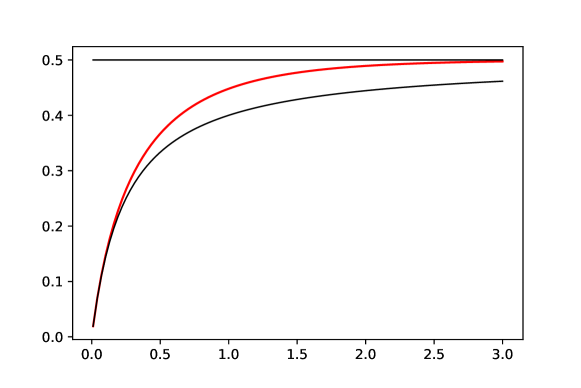
Figure 1: The function $\theta\mapsto\theta i_{\mathfrak{F}}(\theta)$ (red) and its bounds, see (23).

As another, somewhat less straightforward example we consider the family of uniform distributions $P_{\theta}=\text{\rm unif}(0,\theta)$, $\theta\in\Theta:=(0,1)$, on $(S,\mathcal{S})=((0,1),\mathcal{B}_{(0,1)})$ together with the mixture representation in Remark 2. In order to carry out Rao-Blackwellization for the moment estimator $\hat{\theta}=2X$, $X\sim P_{\theta}$, we use the binary representation: For a given $\theta\in\Theta$, let $K(\theta)$, $j_{k}(\theta)$ and $a_{k}(\theta)$ be as in (7). Let $E:=\Theta\cap\mathbb{Q}_{\text{\rm bin}}$, and for $t\in E$ let $d(t):=2^{-K(t)}$ where $K(t)$ is obtained from the binary representation of $t$. Given $\theta\in\Theta$ we assign the weight $w_{\theta}(a_{m}(\theta))=d(a_{m}(\theta))/\theta$ to each $a_{m}(\theta)$, $m=1,\ldots,K(\theta)$, and put $w_{\theta}(t)=0$ otherwise. Further, with each $t\in E$ we associate the mixing distribution $Q(t,\cdot)=\text{\rm unif}(t-d(t),t)$. Then the discrete mixture representation (7) may be written as

$$P_{\theta}=\text{\rm unif}(0,\theta)=\sum_{t\in E}w_{\theta}(t)\,\text{\rm unif}\left(t-d(t),t\right).$$

For example, if $\theta=3/4$ then $K(\theta)=2$, $a_{1}(\theta)=1/2$, $a_{2}(\theta)=3/4$, $d(a_{1}(\theta))=1/2$, $d(a_{2}(\theta))=1/4$, $w_{\theta}(1/2)=2/3$, $w_{\theta}(3/4)=1/3$, and we arrive at

$$\text{\rm unif}\Bigl{(}0,\frac{3}{4}\Bigr{)}\;=\;\frac{2}{3}\,\text{\rm unif}\Bigl{(}0,\frac{1}{2}\Bigr{)}\ +\ \frac{1}{3}\,\text{\rm unif}\Bigl{(}\frac{1}{2},\frac{3}{4}\Bigr{)}.$$

On the product space $(E\times(0,1),\mathcal{P}(E)\otimes\mathcal{B}_{(0,1)})$ we obtain the probability measures $R_{\theta}$ specified by

$$R_{\theta}(\{t\}\times A)=w_{\theta}(t)\,\text{\rm unif}\left(t-d(t),t\right)(A),\ t\in E,\,A\in\mathcal{B}_{(0,1)}.$$

With $T$ and $X$ the canonical projections on $E$ and $(0,1)$ respectively, $T$ is sufficient for $\{R_{\theta}:\theta\in\Theta\}$. For the moment estimator $\hat{\theta}=2X$ conditioning on the sufficient statistic now leads to the estimator $\tilde{\theta}:=E_{\theta}[\hat{\theta}|T]=2T-d(T)$. As in Proposition 12 we first give a general formula and then derive some properties of the function of interest.

Proposition 13.

(a) With the notation as introduced above, the mean squared error of the conditioned moment estimator $\tilde{\theta}=2T-d(T)$ is given by

$$\text{\rm MSE}_{\theta}(\tilde{\theta})=\text{\rm var}_{\theta}(\tilde{\theta})\,=\,\frac{1}{\theta}\sum_{m=1}^{K(\theta)}a_{m}(\theta)a_{m-1}(\theta)\bigl{(}a_{m}(\theta)-a_{m-1}(\theta)\bigr{)}.$$ (24)

(b) The function $\theta\mapsto\phi(\theta):=\text{\rm var}_{\theta}(\tilde{\theta})$ is continuous on $\Theta\setminus E$, and on $E$ it is right continuous and has left hand limits. Moreover,

$$\phi(\theta)-\phi(\theta-)\;=\;-\frac{1}{7q}\,2^{-2L+1}$$ (25)

if $\theta$ is a binary rational of the form $\theta=q2^{-L}$, with $L,q\in\mathbb{N}$ and $q$ odd.

The property ‘right continuous, with left hand limits’ is often abbreviated to ‘càdlàg’.

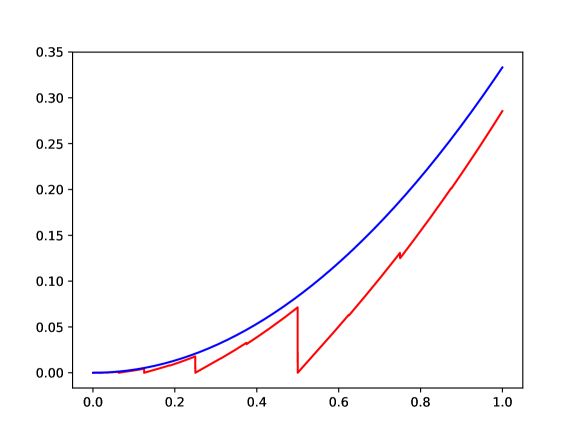
Figure 2: Mean squared errors associated with $\hat{\theta}$ (blue) and $\tilde{\theta}$ (red)

For the unconditioned estimator $\hat{\theta}$ we have $\text{\rm var}_{\theta}(\hat{\theta})=\theta^{2}/3$. Both estimators are unbiased. Figure 2 shows the variances (mean squared errors) of $\hat{\theta}$ and $\tilde{\theta}$ for $\theta$ an integer multiple of $2^{-12}$, with the interpolation justified by Proposition 13 (b). The figure suggests a self-similarity property: Indeed, as $X\sim P_{\theta/2}$ and $2X\sim P_{\theta}$ are equivalent, it follows that both variance functions have the scaling property $\phi(\theta/2)=\phi(\theta)/4$. Further, if $\theta=2^{-m}$ for some $m\in\mathbb{N}$ then the variance is zero, as the distribution of $T$ is degenerate for such values of the parameter.

5.4 An asymptotically efficient estimator for the mean functional

We consider the classical case (19). In the corresponding mixture model we then have

$$\Theta=\Bigl{\{}p=(p_{k})_{k\in\mathbb{N}_{0}}:\,p_{k}\geq 0\text{ for all }k\in\mathbb{N}_{0},\,\sum_{k=0}^{\infty}p_{k}=1\Bigr{\}},$$

and the statistical experiment $\mathfrak{M}$ is based on the family

$$\mathcal{P}\,=\,\Bigl{\{}P_{p}:\,P_{p}=\sum_{k=0}^{\infty}p_{k}\chi_{2k+1}^{2},\,p\in\Theta\Bigr{\}}$$

of mixture distributions parametrized by $p\in\Theta$. The family $\left\{\chi_{1}^{2}(2\theta):\,\theta>0\right\}$ underlying $\mathfrak{F}$ is a subfamily of $\mathcal{P}$.

Our aim is to show that the moment estimator for the mean functional, which we know from the previous subsections to not be efficient in the context of $\mathfrak{F}$, is asymptotically efficient at each $P_{p}\in\mathcal{P}$ that has non-vanishing mixing coefficients with finite variance. We refer the reader to [24, Sections 1.2, 2.1 and 3.1] for an exposition of the general theory needed here. In comparison with the situation in Proposition 12 there are three main differences: First, instead of a parametric family with a parameter $\theta$ specifying the distribution, we now have a one-dimensional parameter function $\kappa:\mathcal{P}\to\mathbb{R}$, where $\kappa(P)$ does not fully characterize $P$. Secondly, instead of the variance of an estimator $\hat{\theta}$ for $\theta$ we now consider the variance of the limiting normal distribution in an associated central limit theorem for a sequence of estimators for $\kappa(P)$. The third point requires some machinery. The basic idea is to consider dominated one-dimensional submodels $\{P_{t}:\,0\leq t<\epsilon\}\subset\mathcal{P}$ with $P_{0}=P$ and then use the derivative at $t=0$, in analogy to (17). This leads to a tangent set, where the geometry is that of a Hilbert space of square integrable functions. Again speaking somewhat informally, a lower bound can then be obtained from the supremum of the associated second moments. Finally, an estimator sequence is said to be asymptotically efficient at $P$ for the parameter function $\kappa$ if asymptotic variance and lower bound are the same for this $P$.

Let $\mathcal{P}_{0}$ be the subset of distributions $P_{p}\in\mathcal{P}$ with $p=(p_{k})_{k\in\mathbb{N}_{0}}$ satisfying the moment condition $\sum_{k=0}^{\infty}k^{2}p_{k}<\infty$ and also the condition that $p_{k}>0$ for each $k\in\mathbb{N}_{0}.$ Consider the mean functional $\kappa:\mathcal{P}_{0}\rightarrow\mathbb{R}$ defined by

$$\kappa(P_{p})=\sum_{k=0}^{\infty}kp_{k},\,P_{p}\in\mathcal{P}_{0}.$$

Let $X_{1},\dots,X_{n},\dots$ be a sequence of independent and identically distributed random variables with distribution $P_{p}\in\mathcal{P}_{0}$ which is assumed to be unknown. Then, generalizing the moment estimator that already appeared in Subsection 5.3,

$$T_{n}:=\frac{1}{2}\bigl{(}\overline{X}_{n}-1\bigr{)}\,=\,\frac{1}{2}\Bigl{(}\frac{1}{n}\sum_{i=1}^{n}X_{i}-1\Bigr{)}$$

leads to a sequence $(T_{n})_{n\in\mathbb{N}}$ of unbiased estimators for $\kappa(P_{p})$, and the central limit theorem shows that, as $n\to\infty$,

$$\sqrt{n}\left(T_{n}-\kappa(P_{p})\right)\xrightarrow{\mathcal{D}}N\Bigl{(}0,v(P_{p})+\kappa(P_{p})+\frac{1}{2}\Bigr{)},$$ (26)

where $v(P_{p})=\sum_{k=0}^{\infty}\left(k-\kappa(P_{p})\right)^{2}p_{k}$.

Theorem 14.

For estimating $\kappa(P_{p}),$ the estimator sequence $(T_{n})_{n=1}^{\infty}$ is asymptotically efficient at each $P_{p}\in\mathcal{P}_{0}$.

If $P_{p}=\chi_{1}^{2}(2\theta)$ then $v(P_{p})=\kappa(P_{p})=\theta$ so that the variance of the limit distribution of $\sqrt{n}\left(T_{n}-\kappa(P_{p})\right)$ is equal to $2\theta+\frac{1}{2}$, in accordance with the value found in Subsection 5.3.

5.5 NPMLE and EM

As we pointed out in the introduction a distribution $P_{\theta}$ with the mixture representation $P_{\theta}=\sum_{i\in E}w_{\theta}(i)\,Q_{i}$ may be seen as the distribution of the outcome $X$ in a two-stage experiment: First, choose $Y$ in $E$ with distribution (mass function) $w_{\theta}$, then, if $Y=i$, choose $X$ according to $Q_{i}$. In a sample $x_{1},\ldots,x_{n}$ of size $n$ from $P_{\theta}$ we may then think of the corresponding $y_{1},\ldots,y_{n}$ as hidden (or latent) variables, or as missing covariates, see [18, Sect. 1.3.5 and 1.3.6]. A non-parametric generalization leads to the problem of estimating the mixing probabilities $p_{i}$, $i\in E$, in a representation $P=\sum_{i\in E}p_{i}\,Q_{i}$ of the unknown distribution $P$, with the $Q_{i}$ known, from the data $x_{1},\ldots,x_{n}$. We may of course regard the sequence $p=(p_{i})_{i\in E}$ as a parameter, where the parameter space is now the probability simplex on $E$, as in the previous subsection.

The EM algorithm, see [4] and [18, Sect. 3.4] can be used to obtain a sequence $p(l)$, $l=1,2,\ldots\,$ of approximations to the corresponding non-parametric maximum likelihood estimator (NPMLE). We give the details for the classical case, where $E=\mathbb{N}_{0}$ and $Q_{k}$ is the central chi-squared distribution with $2k+1$ degrees of freedom, with continuous density $g_{k}$. The log-likelihood function $L_{X}$ is then given by

$$L_{X}(p)\,=\,\sum_{i=1}^{n}\log\Bigl{(}\sum_{k=0}^{\infty}p_{k}\,g_{k}(x_{i})\Bigr{)}.$$ (27)

With the corresponding $y$-values known, the log-likelihood function would be

$$L_{X,Y}(p)\,=\,\sum_{i=1}^{n}\log\bigl{(}p_{y_{i}}\,g_{y_{i}}(x_{i})\bigr{)}\,=\,\sum_{i=1}^{n}\log p_{y_{i}}\,+\,r(x_{1},\ldots,x_{n};y_{1},\ldots,y_{n}),$$ (28)

where the function $r$ does not depend on $p$. In the EM algorithm, we obtain the next approximation $p(l+1)$ for the NPMLE from the current value $p(l)$ as the argmax (M-step) of the conditional expectation (E-step) of $L_{X,Y}(p)$ given $x_{1},\ldots,x_{n}$.

The E-step boils down to the calculation of $E_{p(l)}\bigl{[}\log p_{Y_{i}}|X_{i}=x_{i}\bigr{]}$. Under $P_{p(l)}$ the joint distribution of $X_{i}$ and $Y_{i}$ has density $(x,k)\mapsto p_{k}(l)g_{k}(x)$ with respect to the product of Lebesgue measure on $\mathbb{R}_{+}$ and counting measure on $\mathbb{N}_{0}$, so that the conditional probability of $Y_{i}=k$ given $X_{i}=x$ becomes

$$h_{x}(k)\,=\,\frac{p_{k}(l)\,g_{k}(x)}{\sum_{j=0}^{\infty}p_{j}(l)\,g_{j}(x)},\quad x>0,\,k\in\mathbb{N}_{0}.$$

The M-step then requires maximization of the function

$$p\,\mapsto\,\sum_{k=0}^{\infty}q_{n}(k)\,\log p_{k},\ \text{ with }q_{n}(k):=\frac{1}{n}\sum_{i=1}^{n}h_{x_{i}}(k).$$

As $q_{n}$ is a probability mass function, Gibbs’ inequality can be used to show that the desired argmax is given by $p(l+1)=q_{n}$. Using this in (28) we arrive at

$$p_{k}(l+1)\,=\,\frac{1}{n}\sum_{i=1}^{n}\frac{p_{k}(l)\,g_{k}(x_{i})}{\sum_{j=1}^{\infty}p_{j}(l)\,g_{j}(x_{i})}\quad\text{for all }k\in\mathbb{N}_{0}.$$ (29)

For chi-squared mixing distributions the factors $e^{-x/2}$ cancel in (29) and, more importantly, the infinite sums can be truncated to the range from 0 to

$$K:=K(x_{1},\ldots,x_{n})\,:=\,\bigl{\lceil}(1+\max\{x_{1},\ldots,x_{n}\})/2\bigr{\rceil}.$$

To see this we note that

$$\frac{g_{k-1}(x)}{g_{k}(x)}\;=\;\frac{2\;\Gamma(k+1/2)}{x\;\Gamma(k-1/2)}\;=\,\frac{2k-1}{x}\quad\text{for all }x>0,\,k\in\mathbb{N},$$

Hence, if some $k>K$ appears in (27), then the corresponding mass $p_{k}$ can be shifted to the left without decreasing the value of $L_{X}$ .

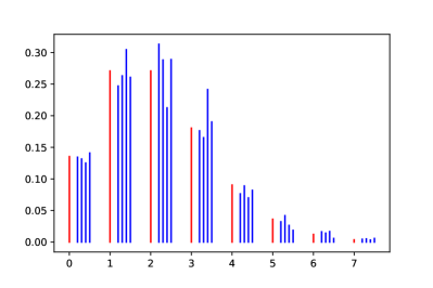
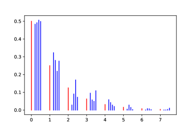
Figure 3: Simulation results (see text)

The left part of Figure 3 shows the results of four simulation experiments, each with $n=10000$ observations, where the base distribution is a noncentral chi-squared with one degree of freedom and noncentrality parameter $\theta=2$. The vertical red lines represent the probability mass $p_{k}$ of the true mixing distribution, which is Poisson with parameter 2, at the positions $k=0,1,\ldots,7$. The four estimates of these masses are computed numerically by using the EM algorithm and are shown in blue slightly to the right.

For noncentral distribution families the nonparametric version incorporates a variant of the deconvolution problem [18, Sect. 1.3.19]: In the chi-squared case, we regard the data as realizations of random variables $X=(Y+Z)^{2}$ with $Y,Z$ independent, $Y$ standard normal, and an unknown distribution $\mu$ for $Z$. The procedure outlined above can be applied and leads to an estimator for the mixed Poisson distribution associated with $\mu$. This in turn can then be used to obtain an estimator for $\mu$, by combining NPMLE and EM again, for example.

The right hand part of Figure 3 shows the results of four simulation experiments where $Z=2\sqrt{W}$ with $W$ exponentially distributed with parameter 1. The corresponding mixed Poisson distribution is the geometric distribution on $\mathbb{N}_{0}$ with parameter $1/2$. Again, the vertical red lines represents the true mixing distribution, the four estimates are slightly to the right and in blue, and each simulation is based on $n=10000$ observations. We should point out that a rather large number $n$ of observations is required in order to obtain estimators with small mean squared error.

Given a sequence $X_{1},\dots,X_{n},\dots$ of independent and identically distributed random variables with distribution $P_{p}=\sum_{k=0}^{\infty}p_{k}\chi_{1+2k}^{2},$ where the parameter $p=(p_{k})_{k\in\mathbb{N}_{0}}$ in the probability simplex on $\mathbb{N}_{0}$ is unknown, the non-parametric maximum likelihood estimator $p_{\rm NPMLE,n}$ of $p$ based on $X_{1},\dots,X_{n}$ exists. Using the general consistency statement given in [19, Theorem 5.3] we deduce that the sequence $(p_{\rm NPMLE,n})_{n\in\mathbb{N}}$ is strongly consistent for $p$.

6 Summary and outlook

We have investigated geometrical and statistical aspects, and their interaction, in the context of discrete mixture representations. It turned out that there are connections to a variety of theoretical and applied topics, including

• tree-based constructions of probability measures, with connections to nonparamnetric Bayesian inference (Theorem 1, Section 5.1),

• the view of mixture representations as curves in an infinite-dimensional space (Section 3),

• Dynkin’s barycentric approach to convexity (Section 4),

• the effect of mixing on Fisher information (Section 5.2) and mean squared error (Section 5.3), and

• algorithmic aspects, notably the use of the EM algorithm (Section 5.5).

We have almost exclusively considered the one-dimensional case, i.e. families of probability distributions on the real line, leaving multivariate situations to a future paper. Another aspect that seems to be worth a separate investigation is the structure of the family $\{Q_{i}:\,i\in E\}$ of mixing distributions in a representation such as (1). In the classical case (12), with noncentral chi-squared distributions, these are the convolution powers of one specific probability measure, and we noted in Remark 3 that the mixing distributions in Theorem 1 constitute a location-scale family of a specific type. Taken together, the multivariate case and the structure of the mixing family are also of interest for applications in the general area of stochastic processes, with relations to the Dynkin isomorphism (see [2, Section 4.2]). In an applied context it would certainly be interesting to remove the assumption in Section 5.5 that the mixing family is known. This would lead to a statistical inverse problem, and structural assumptions could be used, if applicable, to reduce its complexity.

Acknowledgment. We thank the associate editor and the two referees for their detailed and constructive comments, which have led to a considerable improvement of the paper.

Appendix: Proofs

Proof of Theorem 1.  Consider the infinite rooted binary tree where each node has one left and one right descendant. Any $x\in(0,1)$ that is not a binary rational defines a unique infinite path through this tree, starting at the root node, and moving to the left or right descendant if the next digit in its binary expansion is 0 or 1 respectively. With $x=1/3$, for example, we would move to the left and to the right in odd and even steps alternatingly. Our first aim is to obtain a decomposition of $(a,b)\subset(0,1)$ into intervals with binary rational endpoints. For this we label the nodes of tree by appropriately chosen intervals, using (4), and then collect these along the paths given by $a$ and $b$.

In order to carry this out formally, let $a,b\in\mathbb{R}\setminus\mathbb{Q}_{\text{\rm bin}}$, $0<a<b<1$, be given, with binary expansions $a=\sum_{k=1}^{\infty}a_{k}2^{-k}$, $b=\sum_{k=1}^{\infty}b_{k}2^{-k}$ where $a_{k},b_{k}\in\{0,1\}$ for all $k\in\mathbb{N}$. Let $j_{1}<j_{2}<\cdots$ be the positions of the digit 1 in the expansion of $b$. The corresponding partial sums $b(l):=\sum_{k=1}^{j_{l}}b_{k}2^{-k}$, $l\in\mathbb{N}$, then provide a strictly increasing sequence of binary rational numbers with limit $b$. By construction, $2^{j_{l+1}}\bigl{(}b(l+1)-b(l)\bigr{)}=1$, $2^{j_{l+1}}b(l+1)-1$ is even, and $\left(2^{j_{l+1}}b(l+1)-1+2\right)2^{-j_{l+1}}=b(l+1)+2^{-j_{l+1}}>b$.

Similarly, and now writing $j_{1}<j_{2}<\cdots$ for the positions of the digit 0 in the expansion of $a$, and with $a(l):=2^{-j_{l}}+\sum_{k=1}^{j_{l}}a_{k}2^{-k}$, $l\in\mathbb{N}$, we obtain a strictly decreasing sequence $(a(l))_{l\in\mathbb{N}}\subset\mathbb{Q}_{\text{\rm bin}}$ with limit $a$ and the property that $2^{j_{l+1}}a(l+1)$ is odd, and $\left(2^{j_{l+1}}a(l+1)-1\right)2^{-j_{l+1}}=a(l+1)-2^{-j_{l+1}}<a$ for all $l\in\mathbb{N}$.

Let $K:=\min\{k\in\mathbb{N}:\,a_{k}=0,\,b_{k}=1\}$. Clearly, $K<\infty$ as $a<b$. With $a(K):=\sum_{k=1}^{K}a_{k}2^{-k}$, $b(K):=\sum_{k=1}^{K}b_{k}2^{-k}$, we have $(a(K),b(K))\in C(a,b)$, $\bigl{(}a(l+1),a(l)\bigr{)}\in C(a,b)$ for all $l$ with $j_{l}(a)\geq K$, $\bigl{(}b(l),b(l+1)\bigr{)}\in C(a,b)$ for all $l$ with $j_{l}(b)\geq K$, and we finally arrive at the interval decomposition

$$(a,b)=\bigl{(}a(K),b(K)\bigr{)}\;\sqcup\!\!\bigsqcup_{\{l:\,j_{l}(b)\geq K\}}\!\!\bigl{(}b(l),b(l+1)\bigr{)}\;\sqcup\!\!\bigsqcup_{\{l:\,j_{l}(a)\geq K\}}\!\!\bigl{(}a(l+1),a(l)\bigr{)}\;\sqcup\,N,$$

with $N$ countable. This implies

$$(b-a)\,\text{\rm unif}(a,b)\ =\ (b(K)-a(K))\,\text{\rm unif}(a(K),b(K))$$

$$\qquad\qquad+\ \sum_{\{l:\,j_{l}(b)\geq K\}}(b(l+1)-b(l))\,\text{\rm unif}(b(l),b(l+1))$$

$$\qquad\qquad+\ \sum_{\{l:\,j_{l}(a)\geq K\}}(a(l)-a(l+1))\,\text{\rm unif}(a(l+1),a(l)).$$

It remains to remove the restrictions on $a$ and $b$. For elements of $\mathbb{Q}_{\text{\rm bin}}$ the binary representation is not unique, but if we agree to choose the representation with a finite number of digits $1$ in the case of $b$ and a finite number of digits $0$ in the case of $a$ then the only change in the above argument is that the respective sequence of $j$-values would be finite.

In order to remove the assumption $0<a,b<1$ we first describe the way in which the representation interacts with affine transformations $T:\mathbb{R}\to\mathbb{R}$ of the form $T(x)=2^{k}x+r$, with $k\in\mathbb{Z}$ and $r\in\mathbb{Q}_{\text{\rm bin}}$. Such functions are bijections, and their inverse is of the same type. Further, they leave $E$ invariant, if applied to the components of the pair, and it is easy to check that

$$\bigl{(}T(p),T(q)\bigr{)}\in C\bigl{(}T(a),T(b)\bigr{)}\quad\Longleftrightarrow\quad(p,q)\in C(a,b)$$

for all $(a,b)\in\Theta$, $(p,q)\in E$. Hence (5) would imply that

$$\text{\rm unif}\bigl{(}T(a),T(b)\bigr{)}\,=\,\sum_{(p,q)\in E}w_{(T(a),T(b))}(p,q)\,\text{\rm unif}(p,q),$$ (30)

which means that the representation then also holds for $\bigl{(}T(a),T(b)\bigr{)}$. Any pair $(a,b)\in\Theta$ can be transformed by such $T$’s into the unit interval, so the desired representation holds for all $(a,b)\in\Theta$.

Proof of Theorem 4.  It is well-known and follows easily from Shepp’s theorem [7, p.158] that a probability measure $P$ on the positive half-line with weakly decreasing density $f$ (which we may take to be left continuous) may be written as a mixture of uniform distributions on the intervals $[0,y]$, $y>0$. For completeness we give a simple and direct argument: First, a $\sigma$-finite measure $\rho$ on $(\mathbb{R}_{+},\mathcal{B}_{+})$ can be defined via $\rho([y,\infty))=f(y)$ for all $y>0$. Then let $\nu$ be the measure with density $y\mapsto y$ with respect to $\rho$. Is it easy to check that $\nu$ has total mass 1. Also, for all $x>0$,

$$f(x)=\int_{[x,\infty)}\frac{1}{y}\,\nu(dy)=\int_{(0,\infty)}\frac{1}{y}1_{[x,\infty)}(y)\,\nu(dy)=\int_{(0,\infty)}\frac{1}{y}1_{[0,y]}(x)\,\nu(dy),$$

and the integrand in the last expression is a density for $\text{\rm unif}(0,y)$.

With $\mu$ and $f$ as in the statement of the theorem we may write $\mu=\frac{1}{2}(\mu_{0}+\mu_{0}^{T})$ with $T(x)=-x$, and with $\mu_{0}$ a distribution that is concentrated on the positive half-line and has a weakly decreasing density there. Using the first part, we get

$$\mu=\int_{(0,\infty)}\text{\rm unif}(-y,y)\,\nu(dy),$$ (31)

where $\nu$ is the mixing measure for $\mu_{0}$.

We now apply the general principles represented by (8) (repeated mixtures) and (9) (behaviour under push-forwards): First, if $X$ has distribution $\mu$ and $Q_{\theta}$ is the distribution of $X+\theta$, representation (31) implies that

$$Q_{\theta}=\int_{(0,\infty)}\text{\rm unif}(\theta-y,\theta+y)\,\nu(dy).$$ (32)

Thus, the family $\{Q_{\theta}:\,\theta\in\mathbb{R}\}$ has a discrete mixture representation in terms of the countable set of uniform distributions on intervals with binary rational endpoints introduced in connection with Theorem 1. The transfer argument for push-forwards, with $T(x)=|x|$ or $T(x)=x^{2}$, now completes the proof.

Proof of Proposition 6.  Assume without loss of generality that $E=\mathbb{N}$. Let $C:=\sup_{k\in\mathbb{N}}\|Q_{k}\|$. Then, for all $\eta,\theta\in\Theta$,

$$\|P_{\theta}-P_{\eta}\|\ =\ \lim_{K\to\infty}\Bigl{\|}\sum_{k=0}^{K}w_{\theta}(k)Q_{k}-\sum_{k=0}^{K}w_{\eta}(k)Q_{k}\Bigr{\|}$$

$$\leq\ C\,\lim_{K\to\infty}\sum_{k=0}^{K}\bigl{|}w_{\theta}(k)-w_{\eta}(k)\bigr{|}$$

$$\leq\ C\;\|w_{\theta}-w_{\eta}\|_{1}.$$

Proof of Theorem 10.  (a) Suppose that $\mu\in\text{\rm Mix}\{\chi_{1+2k}^{2}:\,k\in\mathbb{N}_{0}\}$ has two mixture representations,

$$\mu\,=\,\sum_{k=0}^{\infty}p_{k}\chi_{1+2k}^{2}\text{ and }\mu\,=\,\sum_{k=0}^{\infty}q_{k}\chi_{1+2k}^{2},$$

with $p_{k},q_{k}\geq 0$ and $\sum p_{k}=\sum q_{k}=1$. Then the respective densities must be equal almost everywhere, so that the continuous versions agree on $(0,\infty)$. This gives

$$\sum_{k=0}^{\infty}\frac{p_{k}}{\Gamma\bigl{(}k+\frac{1}{2}\bigr{)}\,2^{k+\frac{1}{2}}}\,x^{k-\frac{1}{2}}e^{-x/2}\;=\;\sum_{k=0}^{\infty}\frac{q_{k}}{\Gamma\bigl{(}k+\frac{1}{2}\bigr{)}\,2^{k+\frac{1}{2}}}\,x^{k-\frac{1}{2}}e^{-x/2}\text{ for all }x>0.$$

Multiplying both sides by $x^{\frac{1}{2}}e^{x/2}$ and using the uniqueness of the coefficients in a power series representation we get $p_{k}=q_{k}$ for all $k\in\mathbb{N}_{0}$. Hence the mixture representation of elements of $\text{\rm Mix}\{\chi_{1+2k}^{2}:\,k\in\mathbb{N}_{0}\}$ is unique.

Now suppose that $\mu$ is a mixture of noncentral chi-squared distributions with one degree of freedom and mixing measure $\nu$ on the parameter space $\Theta=[0,\infty)$. The classical representation (12) with $n=1$ then gives

$$\mu=\sum_{k=0}^{\infty}p_{k}\chi^{2}_{1+2k}\ \text{ with }p_{k}=\int e^{-\lambda}\frac{\lambda^{k}}{k!}\,\nu(d\lambda)\ \text{ for all }k\in\mathbb{N}_{0},$$

so that the mixing coefficients are the probabilities of a mixed Poisson distribution. In order to prove the strict subset relation it is therefore enough to name a distribution on $\mathbb{N}_{0}$ that is not a mixed Poisson distribution—such as $\delta_{1}$. In particular,

$$\chi_{3}^{2}\;\in\;\text{\rm Mix}\{\chi_{1+2k}^{2}:\,k\in\mathbb{N}_{0}\}\setminus\text{\rm Mix}\{\chi_{1}^{2}(\theta):\,\theta\geq 0\}.$$

To finish the proof of part (a) we use the uniqueness of the representation to show that each $\chi^{2}_{1}(\eta)$, $\eta>0$, is an extreme element of the convex set $\text{\rm Mix}\{\chi_{1}^{2}(\theta):\,\theta\geq 0\}$. Indeed, suppose that $\chi_{1}^{2}(\eta)=\alpha\mu_{1}+(1-\alpha)\mu_{2}$, and that $\nu_{1},\nu_{2}$ are the parameter distributions for $\mu_{1},\mu_{2}$. But then $\chi_{1}^{2}(\eta)$ would itself be a mixture of the distributions $\chi_{1}^{2}(\theta)$, $\theta\geq 0$, with mixing measure $\nu:=\alpha\nu_{1}+(1-\alpha)\nu_{2}$. The uniqueness now implies that $\nu$ is concentrated at $\eta$, so that $\mu_{1}$ and $\mu_{2}$ are equal.

This shows that the set of extreme elements of $\text{\rm Mix}\{\chi_{1}^{2}(\theta):\,\theta\geq 0\}$ is uncountable, in contrast to the set of extreme elements of $\text{\rm Mix}\{\chi_{1+2k}^{2}:\,k\in\mathbb{N}_{0}\}$.

(b) We know from (12) that each $\chi_{k}^{2}(\theta)$, $\theta\geq 0$ and $k\in\mathbb{N}$, has a representation in terms of central chi-squared distributions, so that, by the mixture-of mixtures property (8), the left set is contained in the set on the right side of the assertion. However, $\chi^{2}_{k}=\chi^{2}_{k}(0)$, which means that the mixing distributions are elements of the left set, hence so are their mixtures.

(c) Any element $\mu$ of both sets $\text{\rm Mix}\{\chi_{k+2n}^{2}:\,n\in\mathbb{N}_{0}\}$ and $\text{\rm Mix}\{\chi_{l+2n}^{2}:\,n\in\mathbb{N}_{0}\}$ must have two representations of the form

$$\mu\,=\,\sum_{n=0}^{\infty}p_{n}\chi_{k+2n}^{2}\,\text{ and }\mu\,=\,\sum_{n=0}^{\infty}q_{n}\chi_{l+2n}^{2}.$$

As in the proof of (a) above, this would lead to

$$\sum_{n=0}^{\infty}\frac{p_{n}}{\Gamma\bigl{(}n+\frac{k}{2}\bigr{)}\,2^{n+\frac{k}{2}}}\,x^{n+\frac{k}{2}-1}e^{-x/2}\;=\;\sum_{n=0}^{\infty}\frac{q_{n}}{\Gamma\bigl{(}n+\frac{l}{2}\bigr{)}\,2^{n+\frac{l}{2}}}\,x^{n+\frac{l}{2}-1}e^{-x/2}$$

for all $x>0$. Multiplication by $x^{\frac{1}{2}}e^{x/2}$ and substituting $x=y^{2}$ then gives

$$\sum_{n=0}^{\infty}\frac{p_{n}}{\Gamma\bigl{(}n+\frac{k}{2}\bigr{)}\,2^{n+\frac{k}{2}}}\,y^{2n+k-1}\;=\;\sum_{n=0}^{\infty}\frac{q_{n}}{\Gamma\bigl{(}n+\frac{l}{2}\bigr{)}\,2^{n+\frac{l}{2}}}\,y^{2n+l-1}\text{ for all }y>0.$$

If $k$ and $l$ have different parities then the coefficients of $y$ vanish for all odd powers on one side of the equation, and for all even powers on the other.

Proof of Theorem 11.  (a) On general grounds, the set of extreme elements of $\text{\rm Mix}\{Q_{(p,q)}:\,(p,q)\in E\}$ is a subset of $\{Q_{(p,q)}:\,(p,q)\in E\}$. For an arbitrary $(p,q)=(k2^{m},(k+1)2^{m})\in E$ we have

$$\bigl{(}k2^{m},(k+1)2^{m}\bigr{)}=\bigsqcup_{r=1}^{\infty}\bigl{(}(2^{r+1}k+1)2^{m-r-1},(2^{r+1}k+2)2^{m-r-1}\bigr{)}\;\sqcup\;N$$

with $N$ countable, so that $Q_{(p,q)}$ may be written as

$$Q_{(p,q)}\;=\;\sum_{r=1}^{\infty}2^{-r}\text{\rm unif}\bigl{(}(2^{r+1}k+1)2^{m-r-1},(2^{r+1}k+2)2^{m-r-1}\bigr{)}\ =\ \frac{1}{2}\,\mu_{1}+\frac{1}{2}\,\mu_{2},$$

where $\mu_{1}:=\text{\rm unif}\bigl{(}(4k+1)2^{m-2},(4k+2)2^{m-2}\big{)}$ and

$$\mu_{2}\,:=\,\sum_{r=2}^{\infty}2^{-(r-1)}\text{\rm unif}\bigl{(}(2^{r+1}k+1)2^{m-r-1},(2^{r+1}k+2)2^{m-r-1}\bigr{)}$$

are two different elements of $\text{\rm Mix}\{Q_{(p,q)}:\,(p,q)\in E\}$.

(b) Let $f$ be a density of $\mu$ that is Riemann integrable on all compact intervals. For a fixed $M\in\mathbb{Z}$ consider the partition of the compact interval $I_{M}=[M,M+1]$ into intervals $I_{M,m,k}$, $k=1,\ldots,2^{m}$, of length $2^{-m}$. As these partitions are nested, the step functions $g_{M,m}$, $m\in\mathbb{N}$, given by

$$g_{M,m}:=\sum_{k=1}^{2^{m}}a_{M,m,k}1_{I_{M,k}}\quad\text{ with }a_{M,m,k}:=\inf\bigl{\{}f(x):\,x\in I_{M,m,k}\bigr{\}}$$

are increasing; let $g_{M,\infty}$ be their supremum. Then $0\leq g_{M,\infty}\leq f$, and

$$\int_{I_{M}}g_{M,\infty}\,d\mathfrak{l}=\int_{M}^{M+1}f(x)\,dx=\int_{I_{M}}f\,d\mathfrak{l}$$

as $f$ is Riemann integrable on $I_{M}$. For each of the intervals $D=I_{M,m,k}$ the function $\mathfrak{l}(D)^{-1}1_{D}$ is a density of $\text{\rm unif}(D)$, which is an element of $\text{\rm Mix}\{Q_{(p,q)}:\,(p,q)\in E\}$ by Theorem 1. Further, the differences $g_{M,m+1}-g_{M,m}$ are linear combinations with nonnegative coefficients of the indicators of $I_{M,m+1,k}$, $k=1,\ldots,2^{m+1}$. Taken together this shows that $g_{M,\infty}/\mu(I_{M})$ is the density of an element of $\text{\rm Mix}\{Q_{(p,q)}:\,(p,q)\in E\}$ whenever $\mu(I_{M})>0$. As $\mu$ itself is a mixture of these, an appeal to the repeated mixture property (8) completes the proof of (b).

(c) We start with a familiar construction from measure theory, see e.g.  [3, Problem 2.5 b), p.65]. Let $q_{k}$, $k\in\mathbb{N}$, be an enumeration of the rational numbers in the interval $(0,1)$. Choose for each $k\in\mathbb{N}$ some $n_{k}\in\mathbb{N},\,n_{k}>k+1,$ such that

$$I_{k}:=\left(q_{k}-2^{-n_{k}},q_{k}+2^{-n_{k}}\right)\subset(0,1).$$

Then the union $A:=\bigcup_{k=1}^{\infty}I_{k}$ is a non-empty open subset of $[0,1]$, the Lebesgue measure $\alpha:=\mathfrak{l}(A)$ of which is

$$0<\alpha\leq\sum_{k=1}^{\infty}\mathfrak{l}(I_{k})\leq 2\sum_{k=1}^{\infty}2^{-n_{k}}<\sum_{k=1}^{\infty}2^{-k}=1.$$

The set $A$ is dense in $[0,1]$. Let $\mu$ be the uniform distribution on the complement $[0,1]\setminus A$ of $A$, with density $f:=(1-\alpha)^{-1}(1-1_{A})$. The support of $\mu$ does not contain any interval of positive length, in contrast to the support of the elements of $\text{\rm Mix}\{Q_{i}:\,i\in E\}$.

Proof of Proposition 12.  Denote by $g_{n,\theta}$ the continuous density of the $\chi_{n}^{2}(2\theta)$ distribution, i.e.,

$$g_{n,\theta}(x)=\sum_{k=0}^{\infty}e^{-\theta}\frac{\theta^{k}}{k!}f_{2k+n}(x),~{}x>0.$$

Then

$$\frac{\rm d}{{\rm d}\theta}\log g_{1,\theta}(x)=\frac{g_{3,\theta}(x)-g_{1,\theta}(x)}{g_{1,\theta}(x)},$$

and therefore

$$i_{\mathfrak{F}}(\theta)\,=\,\int_{0}^{\infty}\left(\frac{\rm d}{{\rm d}\theta}\log g_{1,\theta}(x)\right)^{2}g_{1,\theta}(x)\,dx \,=\,\int_{0}^{\infty}\left(\frac{g_{3,\theta}(x)}{g_{1,\theta}(x)}-1\right)^{2}\,g_{1,\theta}(x)\,dx$$

$$\,=\,\int_{0}^{\infty}\left(\frac{g_{3,\theta}(x)}{g_{1,\theta}(x)}\right)^{2}\,g_{1,\theta}(x)\,dx-1.$$

For $\nu\in(-1,\infty)$ let

$$I_{\nu}(x)=(x/2)^{\nu}\sum_{k=0}^{\infty}\frac{(x/2)^{2k}}{k!\Gamma(\nu+k+1)},\ x>0,$$

be the modified Bessel function of the first kind of order $\nu$. Using

$$g_{1,\theta}(x)\; =\;\frac{1}{2}\exp(-\theta-x/2)(x/2\theta)^{-1/4}I_{-1/2}\left((2\theta x)^{1/2}\right),$$

$$g_{3,\theta}(x)\; =\;\frac{1}{2}\exp(-\theta-x/2)(x/2\theta)^{1/4}I_{1/2}\left((2\theta x)^{1/2}\right),$$

see, e.g., [22], we get

$$i_{\mathfrak{F}}(\theta)\,=\,\int_{0}^{\infty}\frac{x}{2\theta}\left(\frac{I_{1/2}\left((2\theta x)^{1/2}\right)}{I_{-1/2}\left((2\theta x)^{1/2}\right)}\right)^{2}g_{1,\theta}(x)\,dx-1.$$

Finally, from $I_{-1/2}(x)=\left(2/(\pi x)\right)^{1/2}\cosh x$ and $I_{1/2}(x)=\left(2/(\pi x)\right)^{1/2}\sinh x$, $x>0$, we deduce that

$$i_{\mathfrak{F}}(\theta) \ =\ \frac{1}{2\theta}\int_{0}^{\infty}x\,\tanh^{2}\left((2\theta x)^{1/2}\right)\,g_{1,\theta}(x)\,dx-1$$

$$\ <\ \frac{1}{2\theta}\int_{0}^{\infty}x\hskip 1.42262ptg_{1,\theta}(x)\,dx-1\quad=\ \frac{1}{2\theta}.$$

The Fisher information in $\mathfrak{E}$ is known to be $i_{\mathfrak{E}}(\theta)=1/\theta$ for $\theta>0$.

To prove the properties of the function $r$ we write

$$r(\theta) \ =\ \frac{1}{2}\int_{0}^{\infty}x\tanh^{2}\bigl{(}(2\theta x)^{1/2}\bigr{)}\,g_{1,\theta}(x)\,dx-\theta$$

$$\ =\ \frac{1}{2}\left(1-s(\theta)\right),$$

with

$$s(\theta)=\int_{0}^{\infty}x\left(1-\tanh^{2}\bigl{(}(2\theta x)^{1/2}\bigr{)}\right)\,g_{1,\theta}(x)\,dx.$$

Noticing that

$$1-\tanh^{2}\bigl{(}(2\theta x)^{1/2}\bigr{)}\ =\ 4\frac{\exp\left(-2(2\theta x)^{1/2}\right)}{\left(1+\exp\left(-2(2\theta x)^{1/2}\right)\right)^{2}}\ \leq\ 4\exp\left(-2(2\theta x)^{1/2}\right)$$

and

$$g_{1,\theta}(x)\ =\ (2\pi x)^{-1/2}e^{-\theta}e^{-x/2}\cosh\left((2\theta x)^{1/2}\right)$$

$$\leq\ (2\pi x)^{-1/2}e^{-\theta}e^{-x/2}\exp\left((2\theta x)^{1/2}\right)$$

we deduce that

$$0\ \leq\ x\left(1-\tanh^{2}\bigl{(}(2\theta x)^{1/2}\bigr{)}\right)\,g_{1,\theta}(x)\ \leq 4(2\pi)^{-1/2}e^{-\theta}x^{1/2}e^{-x/2}.$$

Therefore,

$$0\ \leq\ s(\theta)\leq\ 4(2\pi)^{-1/2}e^{-\theta}\int_{0}^{\infty}x^{1/2}e^{-x/2}\,dx\ =\ 4e^{-\theta},$$

so that $\lim_{\theta\to\infty}s(\theta)=0$. Additionally, due to

$$\lim_{\theta\to 0}x\left(1-\tanh^{2}\bigl{(}(2\theta x)^{1/2}\bigr{)}\right)\,g_{1,\theta}(x)\ =\ xf_{1}(x)\ \text{ for each }x>0,$$

by dominated convergence, we have that $\lim_{\theta\to 0}s(\theta)=\int_{0}^{\infty}xf_{1}(x)\,dx=1$.

Finally, let $0<\theta_{1}<\theta_{2}<\infty$. To show that $s(\theta_{1})>s(\theta_{2})$ we write

$$s(\theta_{1})\ =\ \int_{0}^{\infty}\frac{1-\tanh^{2}\bigl{(}(2\theta_{1}x)^{1/2}\bigr{)}}{1-\tanh^{2}\bigl{(}(2\theta_{2}x)^{1/2}\bigr{)}}\ \frac{g_{1,\theta_{1}}(x)}{g_{1,\theta_{2}}(x)}\ x\left(1-\tanh^{2}\bigl{(}(2\theta_{2}x)^{1/2}\bigr{)}\right)\,g_{1,\theta_{2}}(x)\,dx.$$ (33)

Due to

$$\frac{1-\tanh^{2}\bigl{(}(2\theta_{1}x)^{1/2}\bigr{)}}{1-\tanh^{2}\bigl{(}(2\theta_{2}x)^{1/2}\bigr{)}}\ =\ \frac{\exp\left(-2(2\theta_{1}x)^{1/2}\right)\left(1+\exp\left(-2(2\theta_{2}x)^{1/2}\right)\right)^{2}}{\left(1+\exp\left(-2(2\theta_{1}x)^{1/2}\right)\right)^{2}\exp\left(-2(2\theta_{2}x)^{1/2}\right)}$$

and

$$\frac{g_{1,\theta_{1}}(x)}{g_{1,\theta_{2}}(x)}\ =\ \exp(\theta_{2}-\theta_{1})\frac{\cosh\left((2\theta_{1}x)^{1/2}\right)}{\cosh\left((2\theta_{2}x)^{1/2}\right)}$$

it holds that

$$\frac{1-\tanh^{2}\bigl{(}(2\theta_{1}x)^{1/2}\bigr{)}}{1-\tanh^{2}\bigl{(}(2\theta_{2}x)^{1/2}\bigr{)}}\ \frac{g_{1,\theta_{1}}(x)}{g_{1,\theta_{2}}(x)}\ =\ \exp(\theta_{2}-\theta_{1})\frac{\cosh\left((2\theta_{2}x)^{1/2}\right)}{\cosh\left((2\theta_{1}x)^{1/2}\right)}\ >\ 1$$

for each $x>0$. Thus, by (33), $s(\theta_{1})>s(\theta_{2})$.

Proof of Proposition 13.  (a) Let $\theta\in\Theta$ be given. We first assume that $K(\theta)=\infty$ and suppress the dependence on $\theta$ where convenient. In terms of the sequences $(j_{k})_{k\in\mathbb{N}}$ and $(a_{m})_{m\in\mathbb{N}_{0}}$ we have

$$R_{\theta}(T=a_{m})\,=\,\frac{a_{m}-a_{m-1}}{\theta}\,=\,\frac{1}{\theta 2^{j_{m}}}\quad\text{for all }m\in\mathbb{N}$$

and $R_{\theta}(T=t)=0$ for all other elements $t$ of $E$. Conditionally on $T=a_{m}$, $X$ is uniformly distributed on the interval $(a_{m-1},a_{m}]$. With these definitions we obtain

$$E_{\theta}\tilde{\theta}\ \ =\ \sum_{m=1}^{\infty}R_{\theta}(T=a_{m})E[2X|T=a_{m}]\ =\ \frac{1}{\theta}\sum_{m=1}^{\infty}(a_{m}-a_{m-1})(a_{m}+a_{m-1})$$

$$=\ \frac{1}{\theta}\lim_{M\to\infty}a_{M}^{2}\ =\ \theta,$$

which, of course, is also immediate from the tower property of conditional expectations. Similarly,

$$\theta\,E_{\theta}\tilde{\theta}^{2}\ =\ \sum_{m=1}^{\infty}(a_{m}-a_{m-1})(a_{m}+a_{m-1})^{2}$$

$$=\ \sum_{m=1}^{\infty}(a_{m}^{3}-a_{m-1}^{3})\ +\ \sum_{m=1}^{\infty}a_{m}a_{m-1}(a_{m}-a_{m-1}).$$

From the above expression for $E_{\theta}\tilde{\theta}$ we get $\lim_{m\to\infty}a_{m}^{3}=\theta^{3}$, which completes the proof of (24) in the case that $K(\theta)=\infty$. For binary rational parameter values the same arguments apply, only that the sums are now finite and no limits are needed.

(b) We first consider the function $\Psi(\theta)=w_{\theta}$ that maps $\Theta$ to the set of probability measures on $\mathbb{N}$ together with the total variation distance or, equivalently via probability mass functions, to the space $(\ell_{1}(\mathbb{N}),\|\cdot\|_{1})$. Clearly, $\Psi=\Phi_{1}\circ\Phi_{2}$ where $\Phi_{2}$ maps $\theta=\sum_{k=1}^{\infty}b_{k}2^{-k}$ to the sequence $b(\theta)=(b_{k})_{k\in\mathbb{N}}\in\{0,1\}^{\mathbb{N}}$ of digits in the binary expansion that has infinitely many 0’s, and $\Phi_{1}(b)(\{k\})=b_{k}2^{-k}/\theta$, $k\in\mathbb{N}$. On the intermediate space of 0-1 sequences we consider the product topology, where a sequence of sequences converges if the respective components converge, which here means that the components do not change from some sequence index onwards (which may depend on the index of the component; informally, all components eventually ’freeze’).

The outer function $\Phi_{1}$ is continuous in view of Scheffé’s lemma. For any $\theta\in\Theta\setminus E$ there are infinitely many 0’s (and 1’s) in $b(\theta)$. If $b_{k}(\theta)=0$ and $b_{k+1}(\theta)=1$ then $\theta$ is strictly inside a binary rational interval of length $2^{-k}$. Hence, if $\theta_{n}\to\theta$ then $\theta_{n}$ is also contained in this interval from some $n_{0}$ onwards, which in turn implies that the first $k$ digits remain constant. This shows that the inner function $\Phi_{2}$ is continuous on $\Theta\setminus E$. In a similar fashion we obtain that $\Phi_{2}$ is right continuous on $E$, and that in $E$ its left hand limits exist.

The conditioned estimator $\tilde{\theta}=2T-d(T)$ is bounded. Hence Lebesgue’s dominated convergence theorem can be applied, so that we finally obtain that $\theta\mapsto\text{\rm var}_{\theta}(\tilde{\theta})$ is càdlàg and fully continuous in those parameter values that are not binary rationals.

It remains to prove the formula for the jumps of $\phi$ in binary rationals. Using the notation from the first part of the proof it is clear that $\theta\phi(\theta)$ is the finite sum $\sum_{m=1}^{K}a_{m}a_{m-1}2^{-j_{m}}$, where $j_{1},\dots,j_{K}=L$ are the successive positions of the digit 1 in the (finite) binary expansion of $\theta=q2^{-L}$. Similarly, $\theta\phi(\theta-)$ is the infinite sum $\sum_{m=1}^{\infty}a_{m}^{\prime}a_{m-1}^{\prime}2^{-j_{m}^{\prime}}$ based on the sequence $(j_{m}^{\prime})_{m\in\mathbb{N}}$ with $j_{m}^{\prime}=j_{m}$ for $m<K$, and $j^{\prime}_{K-1+m}=L+m$ for all $m\in\mathbb{N}$. In particular, $a^{\prime}_{m}=a_{m}$ for $m<K$, and we get

$$a^{\prime}_{K-1+m}\,=\,a^{\prime}_{K-1}+2^{-L-1}+\cdots+2^{-L-m}\,=\,a_{K-1}+2^{-L}(1-2^{-m})\ \text{ for all }m\in\mathbb{N}_{0},$$

which leads to

$$\sum_{k=K}^{\infty} a^{\prime}_{k}a^{\prime}_{k-1}(a^{\prime}_{k}-a^{\prime}_{k-1})\ \ =\ \sum_{m=0}^{\infty}a^{\prime}_{K+m}\,a^{\prime}_{K+m-1}\,2^{-j^{\prime}_{K+m}}$$

$$=\ \sum_{m=0}^{\infty}\bigl{(}a_{K-1}+2^{-L}(1-2^{-m-1})\bigr{)}\bigl{(}a_{K-1}+2^{-L}(1-2^{-m})\bigr{)}\,2^{-L-m-1}$$

$$=\ a_{K-1}^{2}\,\sum_{m=0}^{\infty}2^{-L-m-1}$$

$$\hskip 28.45274pt+\ a_{K-1}\,\sum_{m=0}^{\infty}\bigl{(}2^{-L}(1-2^{-m-1})+\;2^{-L}(1-2^{-m})\bigr{)}\,2^{-L-m-1}$$

$$\hskip 28.45274pt+\ \sum_{m=0}^{\infty}2^{-L}(1-2^{-m-1})\,2^{-L}(1-2^{-m})\,2^{-L-m-1}$$

$$=\ a_{K-1}^{2}\,2^{-L}\,+\;a_{K-1}\,2^{-2L}\;+\;\frac{2}{7}\,2^{-3L},$$

hence

$$\theta\,\phi(\theta-)=\,\sum_{k=1}^{K-1}a_{k}a_{k-1}(a_{k}-a_{k-1})\;+\;a_{K-1}^{2}\,2^{-L}\,+\;a_{K-1}\,2^{-2L}\;+\;\frac{2}{7}\,2^{-3L}.$$

From (24) we know that

$$\theta\,\phi(\theta)=\,\sum_{k=1}^{K-1}a_{k}a_{k-1}(a_{k}-a_{k-1})\;+\;a_{K}a_{K-1}(a_{K}-a_{K-1}).$$

Using $a_{K}=\theta$ and $a_{K}-a_{K-1}=2^{-L}$ we now obtain (25) after a short calculation.

Proof of Theorem 14.  Fix $P_{p}\in\mathcal{P}_{0}$. Denote by $\Theta_{d}$ the subset of elements $q=(q_{k})_{k\in\mathbb{N}_{0}}$ in $\Theta$ with finitely many non-zero mixing coefficients $q_{k}.$ For $q=(q_{k})_{k\in\mathbb{N}_{0}}$ in $\Theta_{d}$, $0\leq a<\infty$ and $0\leq t<\min(1,1/a)$ let

$$P_{p,q;a,t}=P_{p}+at(P_{q}-P_{p}).$$

We consider the submodel

$$\mathcal{P}_{p,q;a}=\bigl{\{}P_{p,q;a,t}:\,0\leq t<\min(1,1/a)\bigr{\}}\;\subset\;\mathcal{P}_{0}.$$

Then $v_{p}=\sum_{k=0}^{\infty}p_{k}f_{2k+1}$ is a density of $P_{p}$, and

$$v_{p,q;a,t}=v_{p}+at\sum_{k=0}^{\infty}(q_{k}-p_{k})f_{2k+1}$$

is a density of $P_{p,q;a,t}$, both with respect to the Lebesgue measure $\mathfrak{l}_{+}$ on the Borel subsets of the positive half-line. The partial derivative

$$\dot{v}_{p,q;a,t}=\frac{\partial}{\partial t}v_{p,q;a,t}=a\sum_{k=0}^{\infty}(q_{k}-p_{k})f_{2k+1}$$

does not depend on $t$, hence $t\rightarrow v_{p,\lambda;a,t}^{1/2}$ is continuously differentiable on the interval $[0,\min(1,1/a))$. Note that

$$c_{p,q}:=\max\left(1,\frac{q_{k}}{p_{k}},k\in\mathbb{N}_{0}\right)<\infty,$$

because only finitely many of the $q_{k}$ are non-zero. Due to

$$\frac{\dot{v}_{p,q;a,t}^{2}}{v_{p,q;a,t}}\ =\ a^{2}\frac{\left(\sum_{k=0}^{\infty}q_{k}f_{2k+1}-\sum_{k=0}^{\infty}p_{k}f_{2k+1}\right)^{2}}{(1-at)\sum_{k=0}^{\infty}p_{k}f_{2k+1}+at\sum_{k=0}^{\infty}q_{k}f_{2k+1}}$$

$$\leq\ a^{2}\frac{\left(\sum_{k=0}^{\infty}\frac{q_{k}}{p_{k}}p_{k}f_{2k+1}+\sum_{k=0}^{\infty}p_{k}f_{2k+1}\right)^{2}}{(1-at)\sum_{k=0}^{\infty}p_{k}f_{2k+1}+at\sum_{k=0}^{\infty}q_{k}f_{2k+1}}$$

$$\leq\ a^{2}\frac{(1+c_{p,q})^{2}}{1-at}\sum_{k=0}^{\infty}p_{k}f_{2k+1}(x),$$

dominated convergence can be applied and it follows that the function $t\rightarrow\int\frac{\dot{v}_{p,q;a,t}^{2}}{v_{p,q;t}}\,d\mathfrak{l}_{+}$ is continuous. Thus, $t\rightarrow P_{p,q;a,t}$ is a differentiable path with score function

$$g_{p,q;a}=\frac{\partial}{\partial t}\log v_{p,q;a,t}\Big{|}_{t=0}\;=\;a\left[\frac{\sum_{k=0}^{\infty}q_{k}f_{2k+1}}{\sum_{k=0}^{\infty}p_{k}f_{2k+1}}-1\right],$$

meaning that

$$\bigintss\left[\frac{v_{\theta,q;a,t}^{1/2}-v_{p}^{1/2}}{t}-\frac{1}{2}g_{p,q;a}\hskip 1.42262ptv_{p}^{1/2}\right]^{2}d\mathfrak{l}_{+}\rightarrow 0\ \text{ as }t\to 0,$$

see [24, Lemma 1.8]. The tangent set

$$\dot{\mathcal{P}}_{P_{p}}=\left\{g_{p,q;a}:\,q\in\Theta_{d},\,a\geq 0\right\}$$

of the model $\mathcal{P}_{0}$ at $P_{p}$ is a convex cone. Regarding this cone as a subset of $L_{2}(P_{p})$, we claim that $\tilde{\kappa}_{P_{p}}$ defined by

$$\tilde{\kappa}_{P_{p}}(x)=\frac{1}{2}(x-1)-\kappa(P_{p}),\quad x>0,$$

is an element of the closed linear span $\overline{\rm lin}\dot{\mathcal{P}}_{P_{p}}$ of $\dot{\mathcal{P}}_{P_{p}}$. To see this, we first note that with

$$(2k-1)!!=\begin{cases}1&~{}\text{if}~{}k=0,\\ (2k-1)\cdot(2k-3)\cdots 3\cdot 1&~{}\text{if}~{}k\in\mathbb{N},\end{cases}$$

it holds that

$$f_{2k+1}(x)=\frac{1}{(2k-1)!!}x^{k}f_{1}(x),\hskip 5.69054ptk\in\mathbb{N}_{0}.$$

Thus, for each $r\in\mathbb{N}_{0},$ and $\delta_{r}=(\delta_{rk})_{k\in\mathbb{N}_{0}}$ with $\delta_{rr}=1$ and $\delta_{rk}=0$ otherwise,

$$g_{p,\delta_{r};1}(x)\;=\;\frac{\frac{1}{(2r-1)!!}x^{r}}{\sum_{k=0}^{\infty}\frac{1}{(2k-1)!!}p_{k}x^{k}}\,-\,1,~{}x>0.$$

Putting

$$a_{0} =-\left(\kappa(P_{p})+\frac{1}{2}\right)p_{0},$$

$$a_{k} =\frac{1}{2}(2k-1)p_{k-1}-\left(\kappa(P_{p})+\frac{1}{2}\right)p_{k},~{}k\in\mathbb{N},$$

it follows that

$$\tilde{\kappa}_{P_{p}}(x)=\sum_{k=0}^{\infty}a_{k}g_{p,\delta_{k};1}(x),~{}x>0,$$

where the series converges pointwise and in $L_{2}(P_{p}).$ Therefore, as asserted, $\tilde{\kappa}_{P_{p}}\in\overline{\rm lin}\dot{\mathcal{P}}_{P_{p}}$. Due to

$$\kappa(P_{p,q;a,t})-\kappa(P_{p})=t\int\tilde{\kappa}_{P_{p}}\,g_{p,q;a}\,dP_{p}$$

for each $q\in\Theta_{d}$, each $a\geq 0$ and each $0\leq t<\min(1,1/a)$, the functional $\kappa$ is differentiable at $P_{p}$ relative to the tangent cone $\dot{\mathcal{P}}_{P_{p}}$. Hence $\tilde{\kappa}_{P_{p}}$ is the efficient influence function for estimating the functional $\kappa$ at $P_{p}$. By (26) and Lemma 2.9 in [24], the sequence of estimators $(T_{n})_{n=1}^{\infty}$ for estimating $\kappa$ is thus asymptotically efficient at $P_{p}$.

References

• [1] Amari, Shun-Ichi (1982). Differential geometry of curved exponential families—curvature and information loss. Ann. Stat. 10, 357-385.
• [2] Baringhaus, L. and Grübel, R. (2020). Mixture representations of noncentral distributions. Published online in Comm. Statist. Theory Methods. DOI: 10.1080/03610926.2020.1738487.
• [3] Benedetto, J.J. (1976). Real variable and integration. Teubner, Stuttgart.
• [4] Dempster, A. P., Laird, N. M. and Rubin, D. B. (1977). Maximum likelihood from incomplete data via the EM algorithm. J. Roy. Statist. Soc. Ser. B 39, 1–38.
• [5] Dynkin, E. B. (1978). Sufficient statistics and extreme points. Ann. Prob. 6, 705–730.
• [6] Efron, B. (1975). Defining the curvature of a statistical problem (with applications to second order efficiency). Ann. Stat. 3, 1189–1242.
• [7] Feller, W. (1971). An Introduction to Probability Theory and Its Applications, Vol. II, 2nd ed. Wiley, New York.
• [8] Ferguson, T.S. (1974). Prior distributions on spaces of probability measures. Ann. Statist. 2, 615–629.
• [9] Ghosal, S. and van der Vaart, A. (2017). Fundamentals of Nonparametric Bayesian Inference. Cambridge University Press, Cambridge.
• [10] Goel, P.K. and DeGroot, M.H. (1979). Comparison of experiments and information measures. Ann. Statist. 7, 1066–1077.
• [11] Grenander, Ulf (1956). On the theory of mortality measurement II. Skand. Aktuarietidskr. 39, 125–153.
• [12] Hoff, Peter D. (2003). Nonparametric estimation of convex models via mixtures, Ann. Statist. 31, 174–200.
• [13] Kubokawa, T., Marchand, É. and Strawderman, W. E. (2017). A unified approach to estimation of noncentrality parameters, the multiple correlation coefficient, and mixture models. Math. Methods Statist. 26, 134–148.
• [14] Lauritzen, S. (1988). Extremal families and systems of sufficient statistics. Lecture Notes in Statistics 49. Springer, Heidelberg.
• [15] Le Cam, L. (1996). Comparison of experiments - a short review. Statistics, probability and game theory, 127–138. IMS Lecture Notes Monogr. Ser., 30. Inst. Math. Statist. Hayward, CA.
• [16] Lehmann, E. L. and Casella, G. (1998). Theory of Point Estimation, second edition. Springer-Verlag, New York.
• [17] Leroux, Brian G. (1992). Consistent estimation of a mixing distribution, Ann. Statist. 20, 1350–1360.
• [18] Lindsay, B. G. (1995). Mixture Models: Theory, Geometry and Applications. NSF-CBMS Regional Conference Series in Probability and Statistics, Volume 5. IMS, Hayward.
• [19] Pfanzagl, J. (1988). Consistency of maximum likelihood estimators for certain nonparametric families, in particular: mixtures. J. Statist. Plann. Inference 19, 137–158.
• [20] Phelps, Robert R. (2001). Lectures on Choquet’s theorem, second edition. Lecture Notes in Mathematics 1757, Springer-Verlag, Berlin.
• [21] Rudin, W. (1991). Functional Analysis. McGraw-Hill, New York.
• [22] Saxena, K. M. L. and Alam, K. (1982). Estimation of the noncentrality parameter of a chi squared distribution. Ann. Statist. 10, 1012–1016.
• [23] Stone, M. (1961). Non-equivalent comparisons of experiments and their use for experiments involving location parameters. Ann. Math. Statist. 32, 326–332.
• [24] van der Vaart, A. (2002). Semiparametric statistics. In: Bolthausen, E., Perkins, E. and van der Vaart, A. Lectures on Probability Theory and Statistics. Lecture Notes in Mathematics 1781, Springer, Berlin.
• [25] Wood, G. R. (1992). Binomial mixtures and finite exchangeability, Ann. Probab. 20, 1167–1173.
• [26] Wood, G. R. (1999). Binomial mixtures: geometric estimation of the mixing distribution, Ann. Statist. 27, 1706–1721.