Optically enhanced discharge excitation and trapping of ³⁹Ar

Abstract

We report on a two-fold increase of the ³⁹Ar loading rate in an atom trap by enhancing the generation of metastable atoms in a discharge source. Additional atoms in the metastable $1s_{5}$ level (Paschen notation) are obtained via optically pumping both the $1s_{4}-2p_{6}$ transition at $801\text{\,}\mathrm{n}\mathrm{m}$ and the $1s_{2}-2p_{6}$ transition at $923\text{\,}\mathrm{n}\mathrm{m}$. By solving the master equation for the corresponding six-level system, we identify these two transitions to be the most suitable ones and encounter a transfer process between $1s_{2}$ and $1s_{4}$ when pumping both transitions simultaneously. We calculate the previously unknown frequency shifts of the two transitions in ³⁹Ar and confirm the results with trap loading measurements. The demonstrated increase in the loading rate enables a corresponding decrease in the required sample size, uncertainty and measurement time for ³⁹Ar dating, a significant improvement for applications such as dating of ocean water and alpine ice cores.

I Introduction

The noble gas radioisotope ³⁹Ar with a half-life of $268\pm 8\text{\,}\mathrm{y}\mathrm{e}\mathrm{a}\mathrm{r}\mathrm{s}$ [1, 2] has long been identified as an ideal dating isotope for water and ice in the age range 50-$1800\text{\,}\mathrm{y}\mathrm{e}\mathrm{a}\mathrm{r}\mathrm{s}$ due to its chemical inertness and uniform distribution in the atmosphere [3, 4]. However, its extremely low isotopic abundances of $10^{-17}-10^{-15}$ in the environment have posed a major challenge in the analysis of ³⁹Ar. In the past, it could only be measured by Low-Level Counting, which requires several tons of water or ice [5].
In recent years, the sample size for ³⁹Ar dating has been drastically reduced by the emerging method Atom Trap Trace Analysis (ATTA), which detects individual atoms via their fluorescence in a magneto-optical trap (MOT). This laser-based technique was originally developed for ⁸¹Kr and ⁸⁵Kr [6, 7, 8, 9] and has later been adapted to ³⁹Ar, realizing dating of groundwater, ocean water and glacier ice [10, 11, 12, 13]. The latest state-of-the-art system reaches an ³⁹Ar loading rate of $\sim$$10\text{\,}\mathrm{a}\mathrm{t}\mathrm{o}\mathrm{m}\mathrm{s}\mathrm{/}\mathrm{h}$ for modern samples and an ³⁹Ar background of $\sim$$0.1\text{\,}\mathrm{a}\mathrm{t}\mathrm{o}\mathrm{m}\mathrm{s}\mathrm{/}\mathrm{h}$ [14, 15]. Still, its use in applications like ocean circulation studies and dating of alpine glaciers is hampered by the low count rate, which determines the measurement time, precision and sample size.
Laser cooling and trapping of argon atoms in the ground level is not feasible due to the lack of suitable lasers at the required vacuum ultra violet (VUV) wavelength. As it is the case for all noble gas elements, argon atoms need to be excited to the metastable level $1s_{5}$ where the $1s_{5}-2p_{9}$ cycling transition at $811\text{\,}\mathrm{n}\mathrm{m}$ can be employed for laser cooling and trapping (Paschen notation [16] is used here, the corresponding levels in Racah notation [17] can be found in Fig. 7 in Appendix A). The $1s_{5}$ level is $\sim$$10\text{\,}\mathrm{e}\mathrm{V}$ above the ground level and, in operational ATTA instruments, is populated by electron-impact excitation in a RF-driven discharge with an efficiency of only $10^{-4}-10^{-3}$. Increasing this efficiency would raise the loading rate of ³⁹Ar accordingly.
Since the discharge excites atoms into not only the metastable $1s_{5}$ but also many other excited levels, the metastable $1s_{5}$ population can be enhanced by transferring atoms from these other excited levels to the metastable $1s_{5}$ via optical pumping (Fig. 1). This mechanism has been demonstrated in a spectroscopy cell for argon with an increase of 81% [18, 19] and for xenon with an increase by a factor of 11 [20, 21]. It has also been observed in an argon beam with an increase of 21% [18]. While these experiments were done on stable and abundant isotopes, a $60\text{\,}\%$ increase in loading rate has recently been observed for the rare isotopes ⁸¹Kr and ⁸⁵Kr [22].
In this work, we theoretically and experimentally examine the enhancement of metastable production by optical pumping for the rare ³⁹Ar as well as the abundant argon isotopes. We identify the $1s_{4}-2p_{6}$ transition at $801\text{\,}\mathrm{n}\mathrm{m}$ and the $1s_{2}-2p_{6}$ transition at $923\text{\,}\mathrm{n}\mathrm{m}$ as the most suitable candidates. Implementing the enhancement scheme for ³⁹Ar on these transitions requires knowing the respective frequency shifts, which we calculate and experimentally confirm. Moreover, loading rate measurements support the theoretically predicted transfer process between $1s_{2}$ and $1s_{4}$ levels when driving the 923-nm and 801-nm transitions simultaneously.

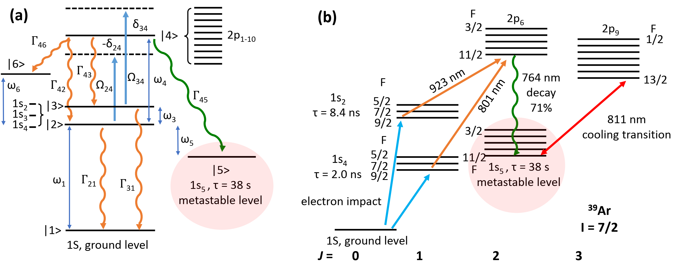
Figure 1: (a) Scheme for enhancing the population in the metastable level $1s_{5}$ by driving the $1s-2p$ levels with Rabi frequencies $\Omega_{24}$, $\Omega_{34}$ and detunings $\delta_{24}$, $\delta_{34}$. $\Gamma_{ij}$ denotes the spontaneous emission rate from level $i$ to $j$. (b) The optical pumping scheme chosen in this work on the $1s_{4}-2p_{6}$ transition at $801\text{\,}\mathrm{n}\mathrm{m}$ and $1s_{2}-2p_{6}$ transition at $923\text{\,}\mathrm{n}\mathrm{m}$, shown for ³⁹Ar which has a nuclear spin $I=7/2$.

I.1 Transfer efficiency

We solve the Lindblad master equation (see details in Appendix B) for the 6-level system shown in Fig. 1(a) which corresponds to the even argon isotopes without hyperfine structure. The resulting steady-state solution $\widetilde{\rho}_{55}(t\to+\infty)$ for the final population in the metastable level can be obtained analytically as a function of the initial populations in ${\left|2\right\rangle}$ and ${\left|3\right\rangle}$, using the initial condition

$$\widetilde{\rho}_{ij}(t=0)=0\text{\ \ for \ }(i,j)\not=(2,2)\ \text{and}\ (i,j)\not=(3,3).$$ (1)

If only one transition is driven, e.g. $\Omega_{34}=0$, then $\widetilde{\rho}_{55}(t\to+\infty)$ simplifies to the expressions given in [22]. We use these expressions to calculate the transfer efficiency $\widetilde{\rho}_{55}(t\to+\infty)$ for the different $1s-2p$ transitions in even argon isotopes as a function of laser power. The transitions with the highest transfer efficiencies are shown in Table 1 (see Table 3 in Appendix C for all transitions).

Table 1: Argon transitions with the highest transfer efficiencies from each $1s$ level, calculated for a laser beam of 9-mm diameter and different powers $P$. For driving both transitions simultaneously (bottom row) an equal population in $1s_{2}$ and $1s_{4}$ and equal power $P$ for each laser beam is assumed.

Lower level	Upper level	$\lambda$\text{\,}\mathrm{(}\mathrm{n}\mathrm{m}\mathrm{)}$$	$\widetilde{\rho}_{55}(t\to+\infty)$
			$P=$0.5\text{\,}\mathrm{W}$$	$P\rightarrow+\infty$\text{\,}\mathrm{W}$$
$1s_{4}$	$2p_{6}$	801	0.03	0.05
$1s_{3}$	$2p_{10}$	1047	0.77	0.77
$1s_{2}$	$2p_{6}$	923	0.15	0.17
$1s_{2}+1s_{4}$	$2p_{6}$	801+923	0.12	0.08

From the metastable level $1s_{3}$ (see Fig. 7 in Appendix C), the $1s_{3}-2p_{10}$ transition at $1047\text{\,}\mathrm{n}\mathrm{m}$ has the highest transfer efficiency of $77\text{\,}\%$. Since $1s_{3}$ is also metastable, only a few mW of laser power are needed to saturate the transition. However, experimentally we only achieve an increase in the metastable $1s_{5}$ population of $\sim$$10\text{\,}\%$ by pumping this transition. Since the increase in the population of the metastable $1s_{5}$ is the product of the transfer efficiency (=0.77, Table 1) and the initial population in the $1s_{3}$, it follows that the latter is only $10\%/0.77=13\%$ of that in the metastable $1s_{5}$. Given this limitation, optical pumping on $1s_{3}$ is not investigated further in this work.
The transfer efficiency from $1s_{2}$ is the highest for the 923-nm transition to $2p_{6}$, reaching a high-power limit of $17\text{\,}\%$. From $1s_{4}$ the transfer efficiency is the highest for the 801-nm transition to $2p_{6}$, reaching a high-power limit of $5\text{\,}\%$. Since the populations of these levels in the argon discharge are not known, the actual increase in the metastable population needs to be determined experimentally. In the following we focus on these two transitions as illustrated in Fig. 1(b) for the odd isotope ³⁹Ar.

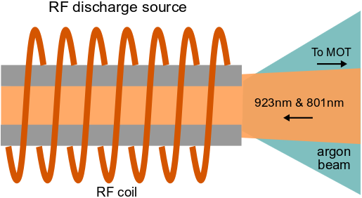
Figure 2: RF-driven discharge source of metastable argon atoms in the ATTA setup. The optical pumping laser beams are sent into the source counter-propagating to the atomic beam.

((a))

((b))

Figure 3: Gain in the MOT loading rate for the abundant argon isotopes vs frequency of the (a) 801-nm and (b) 923-nm optical pumping light, measured in the enriched sample. For each transition, $f_{40}$ denotes the resonance frequency of ⁴⁰Ar at rest as monitored in a spectroscopy cell.

Interestingly, when these two transitions are driven simultaneously (i.e. $\Omega_{24}\neq 0,\Omega_{34}\neq 0$) the final population in the metastable level $\rho_{55}$ is smaller than the sum of the individually driven transitions (see bottom row of table 1). This effect is the consequence of stimulated emission from $2p_{6}$ to $1s_{4}$ by the 801-nm light, together with the 923-nm light effectively transferring atoms from $1s_{2}$ to $1s_{4}$. In the same way atoms are also transferred from $1s_{4}$ to $1s_{2}$. However, since the decay rate to the ground level from $1s_{4}$ is three times higher than from $1s_{2}$ (see Fig. 7 in Appendix A), the total increase in the metastable level is lower than the sum of the individually driven transitions. As the laser power increases also the stimulated emission increases, leading to a further decrease in the combined transfer efficiency to the metastable level.

I.2 Isotope shifts and hyperfine splittings for ³⁹Ar

The total frequency shifts of ³⁹Ar for the 801-nm and 923-nm transitions consist of the isotope shifts and the hyperfine splittings. The hyperfine coefficients of ³⁹Ar for $1s_{2}$ and $1s_{4}$ were measured in [23], whereas for $2p_{6}$ they can be calculated from the corresponding hyperfine coefficients measured for ³⁷Ar [24], using the measured nuclear magnetic dipole moments and electric quadrupole moments of ³⁹Ar and ³⁷Ar [25, 22, 26, 24]. The resulting hyperfine coefficients are shown in Table 5 in Appendix D. Isotope shifts of neither the 801-nm transition nor the 923-nm transition for any argon isotope have been found in the literature. The isotope shifts for ³⁶Ar and ³⁸Ar have therefore been measured in this work (see below), allowing us to calculate the isotope shifts for ³⁹Ar [27, 28, 22]. The resulting isotope shifts and hyperfine splittings for ³⁹Ar relative to ⁴⁰Ar are given in Table 6 in Appendix D.

II Experimental Setup

For measuring the metastable population increase by optical pumping in ³⁹Ar as well as the stable argon isotopes, we use an ATTA system as described in [14]. Metastable argon atoms are generated in a RF-driven discharge by electron impact (Fig. 2) and are subsequently laser cooled and detected in a magneto-optical trap. Single ³⁹Ar atoms are detected via their 811-nm fluorescence in the MOT using an electron-multiplying charged coupled device (EMCCD) camera. During a measurement of ³⁹Ar (³⁹Ar/Ar=$8\times 10^{-16}$ in modern air), the stable and abundant ³⁸Ar (³⁸Ar/Ar=$0.06\text{\,}\%$ in air) is measured as well to account for drifts in the trap loading efficiency. The loading rate of ³⁸Ar for this normalization purpose is measured by depopulating the MOT with a quenching transition and detecting the emitted fluorescence [7, 14]. For testing optical pumping on ³⁸Ar and the other stable argon isotopes the loading rate is measured by first clearing the MOT with a quenching transition and then the initial linear part of the rising slope of the MOT fluorescence is measured [29].
For optical pumping, we shine in the $923\text{\,}\mathrm{n}\mathrm{m}$ and $801\text{\,}\mathrm{n}\mathrm{m}$ laser beams counter-propagating to the atomic beam (Fig. 2). The laser beams are weakly focused and slightly larger than the inner diameter of the source tube (⌀$10\text{\,}\mathrm{m}\mathrm{m}$).

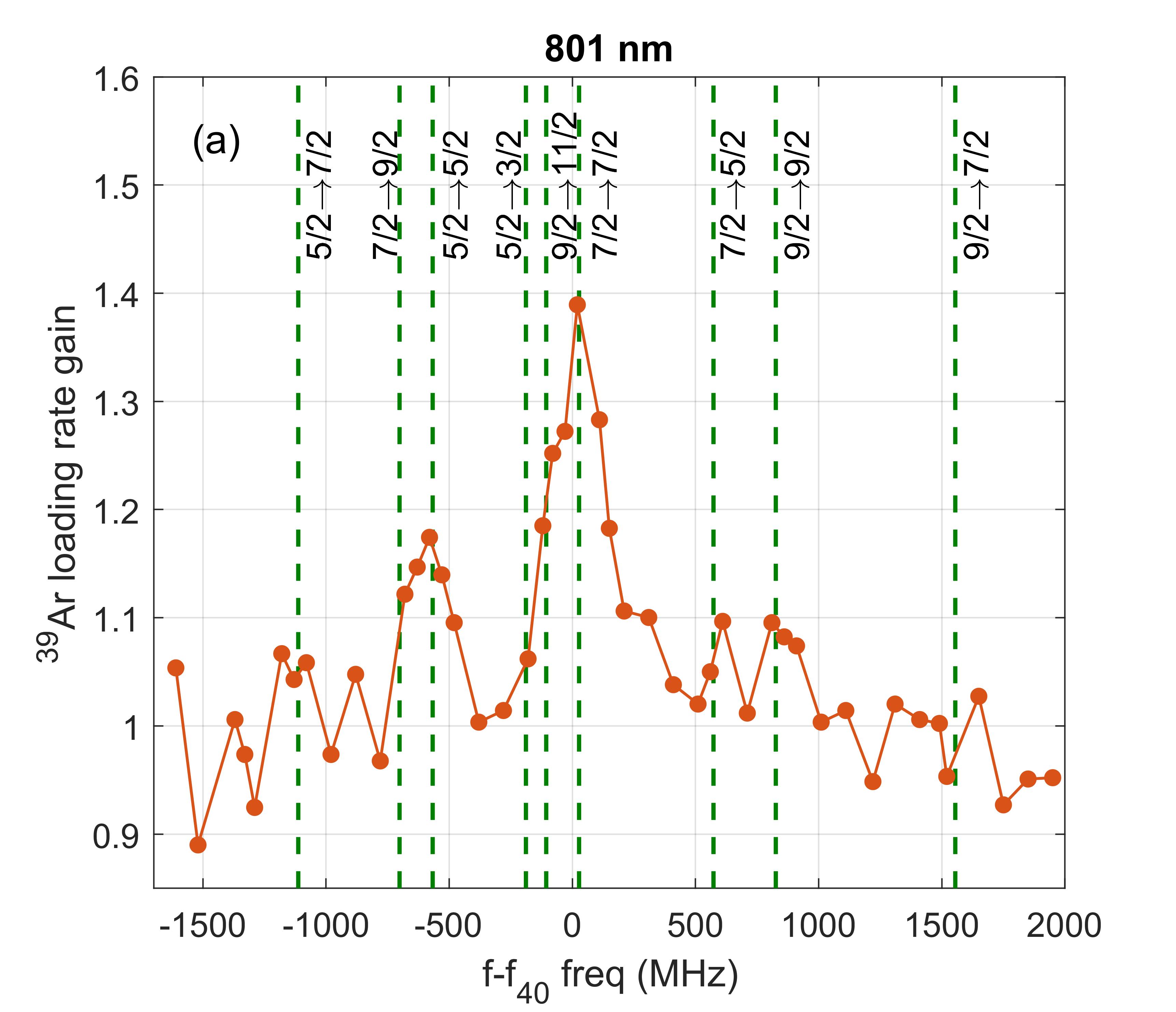
((a))

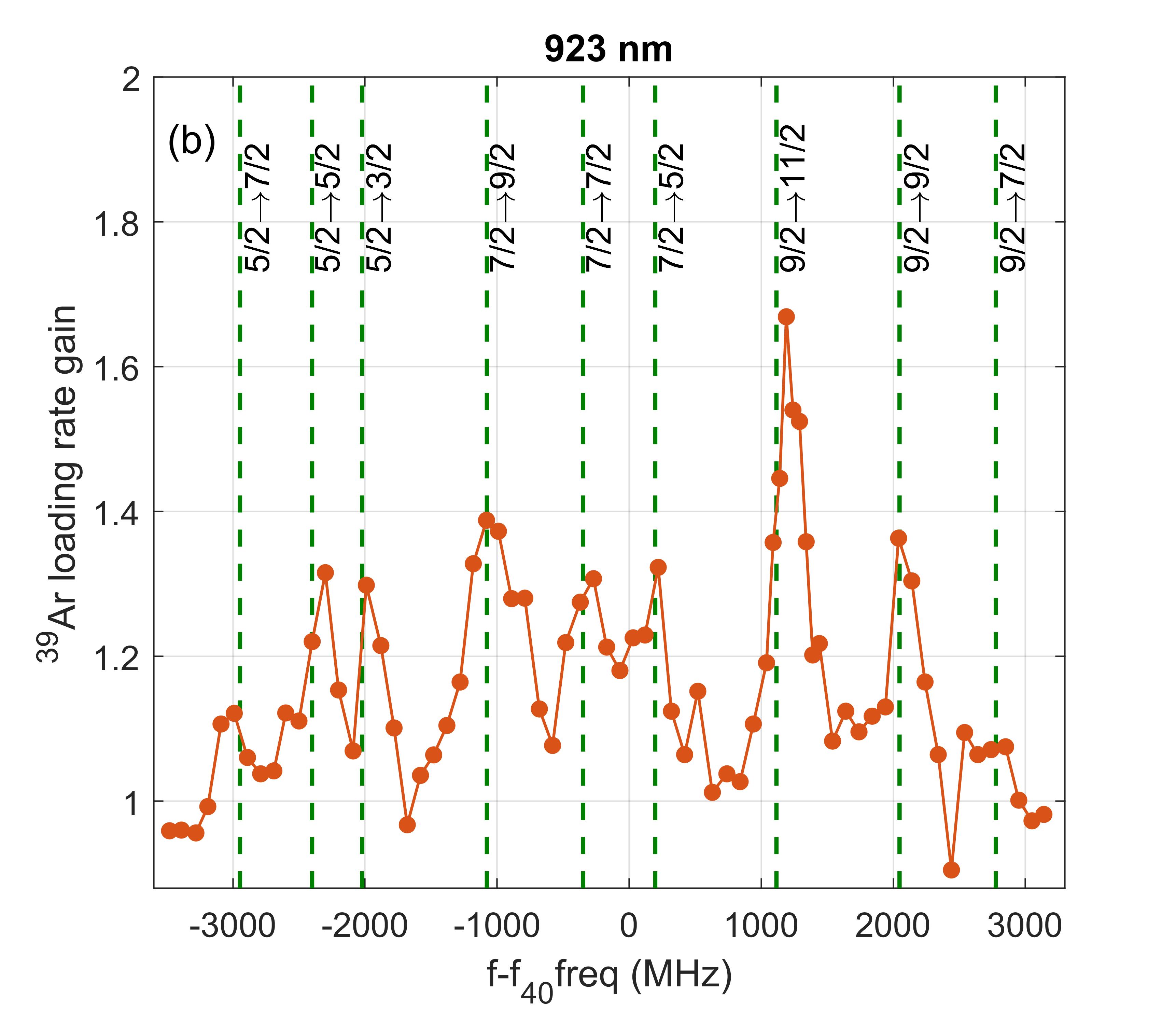
((b))

Figure 4: ³⁹Ar loading rate gain versus frequency of the (a) 801-nm and (b) 923-nm light, measured in the enriched sample. $f_{40}$ denotes the resonance frequency of ⁴⁰Ar at rest as monitored in a spectroscopy cell. The Doppler-shift obtained for ⁴⁰Ar has been subtracted from the frequency to obtain the ³⁹Ar frequency spectrum at rest. The error of each ³⁹Ar data point is $\sim$$5\text{\,}\%$. The dashed green lines indicate the calculated frequencies of the hyperfine transitions.

The optical pumping light is generated by tapered amplifiers seeded with diode lasers, providing up to $1.0\text{\,}\mathrm{W}$ of usable laser power at $801\text{\,}\mathrm{n}\mathrm{m}$ and $1.6\text{\,}\mathrm{W}$ at $923\text{\,}\mathrm{n}\mathrm{m}$. For measuring the different argon isotopes, the laser frequency needs to be tuned and stablilized over several GHz. For this purpose, the two lasers are locked by a scanning transfer cavity lock [30, 31], using a diode laser locked to the 811-nm cooling transition of metastable ⁴⁰Ar as the master. In order to increase counting statistics for ³⁹Ar, we use an enriched sample prepared by an electromagnetic mass separation system [32]. In the enriched sample, ⁴⁰Ar is largely and ³⁶Ar partially removed so that ³⁹Ar and ³⁸Ar are enriched by a factor $\sim 200$. The ratio of ³⁹Ar and ³⁸Ar is not changed in the enrichment process [33], which is important for the normalization described above. The ⁴⁰Ar, ³⁶Ar and ³⁸Ar abundances in the enriched sample are $60\text{\,}\%$, $30\text{\,}\%$ and $10\text{\,}\%$, respectively.

III Results and Discussion

The loading rate of the stable argon isotopes is measured versus the frequencies of the 801-nm and 923-nm light (Fig. 3). A clear increase in the loading rate is observed for all isotopes. For ⁴⁰Ar we obtain most probable Doppler shifts around $-230\text{\,}\mathrm{M}\mathrm{H}\mathrm{z}$ in agreement with the expected temperature of the liquid-nitrogen-cooled atomic beam. The small ⁴⁰Ar feature mirrored on the positive detuning side is likely caused by the optical pumping light reflected at the window behind the source. The window is partially coated by metal which has been sputtered by argon ions that are produced in the discharge. From the observed resonances for ³⁶Ar and ³⁸Ar we obtain the isotope shifts with respect to ⁴⁰Ar for the 801-nm as well as the 923-nm transition shown in Table 4. Based on these measured isotope shifts, we calculate the isotope shifts for ³⁹Ar (Table 4) using King plots [27]. Interestingly, the loading rate of ³⁶Ar shows a pronounced increase also at the ⁴⁰Ar resonance for both, the 801-nm and the 923-nm transition. Looking closely, an increase in loading rate is visible for each isotope at the resonances of the other two isotopes. This additional increase is likely caused by metastable exchange collisions, e.g. transferring an increase in the metastable population of ⁴⁰Ar to that of ³⁶Ar. The maximum loading rate gain is lower for ⁴⁰Ar than for the less abundant ³⁶Ar and ³⁸Ar. This difference is discussed in more detail below.

((a))

((b))

Figure 5: (a) Loading rate gain of the argon isotopes vs laser power of the (a) 801-nm light and (b) 923-nm light, measured with the enriched argon sample. The lines are saturation fits according to the expressions given in [22].

Fig. 4 shows the ³⁹Ar loading rate gain vs frequency of the 801-nm and 923-nm light. For both transitions, a clear increase in the loading rate is observed. For $923\text{\,}\mathrm{n}\mathrm{m}$, the $F=9/2\rightarrow 11/2$ transition is the strongest as expected from the multiplicity and transition strength [34]. Moreover, the measurements confirm the other calculated hyperfine transitions. For $801\text{\,}\mathrm{n}\mathrm{m}$, the overlap of the $F=9/2\rightarrow 11/2$ and $F=7/2\rightarrow 7/2$ transition is the strongest. The loading rate increase is lower compared to that achieved with the 923-nm light. Accordingly, the different hyperfine transitions are resolved less clearly. Nevertheless, the measurements are in good agreement with the calculated hyperfine transitions. In order to address not only one but two hyperfine levels of ³⁹Ar, we add sidebands to the 801-nm and 923-nm light. At $801\text{\,}\mathrm{n}\mathrm{m}$ no increase is detectable by adding a sideband resonant with the overlap of the $F=7/2\rightarrow 9/2$ and $F=5/2\rightarrow 5/2$ transitions. At $923\text{\,}\mathrm{n}\mathrm{m}$ we observe a maximum increase of only $\sim$$10\text{\,}\%$, although according to Fig. 4(b) an increase of $40\text{\,}\%$ appears possible. Likely, the increase by adding a sideband is compensated by the decrease due to the lower laser power on the carrier frequency.
The loading rate gain as a function of laser power is shown in Fig. 5. As already observed in Fig. 3(a), the maximum loading rate gain is lower for ⁴⁰Ar than for the less abundant ³⁶Ar and ³⁸Ar. This may be caused by the higher density of ⁴⁰Ar leading to a stronger trapping of the $764\text{\,}\mathrm{n}\mathrm{m}$ fluorescence (see Fig. 1), which can quench other metastable atoms. Moreover, the saturation intensity is significantly lower for ⁴⁰Ar than for ³⁶Ar and ³⁸Ar. This may also be caused by the higher density of ⁴⁰Ar, leading to trapping of the re-emitted 801-nm and 923-nm light. The saturation intensity for ³⁹Ar is difficult to assess due to the large measurement uncertainties and the contribution from neighbouring hyperfine levels.
Table 2 lists the maximum loading rate gains of the different argon isotopes for the 801-nm and the 923-nm transitions, as well as for both transitions driven together. As predicted by the calculation in section I.1 and Appendix B, driving

Table 2: Loading rate gains obtained for different argon isotopes and different transitions, measured in the enriched argon sample.

Isotope	$801\text{\,}\mathrm{n}\mathrm{m}$	$923\text{\,}\mathrm{n}\mathrm{m}$	$801\text{\,}\mathrm{n}\mathrm{m}$ + $923\text{\,}\mathrm{n}\mathrm{m}$
40Ar	1.4	1.7	1.8
38Ar	1.6	2.5	2.8
36Ar	1.6	2.2	2.6
39Ar	1.4	1.8	2.0

both transitions simultaneously results in a lower gain than the addition of the individual gains. This result confirms the transfer due to stimulated emission between $1s_{2}$ and $1s_{4}$ via the intermediate $2p_{6}$, driven by the 923-nm and 801-nm light. For ³⁹Ar a two-fold gain in the loading rate is obtained by optical pumping when simultaneously using 801-nm and 923-nm light and addressing the $F=9/2$ level. According to the loading rate gain obtained for the other hyperfine levels (Fig. 4), if sidebands are introduced with additional laser power a near three-fold gain in the loading rate should be possible.
As mentioned above and observed in Fig. 5, the loading rate gain varies for different isotopes. Moreover, we observe that the loading rate gain depends on density and sample composition. In order to examine the dependence, we measure the ³⁶Ar and ⁴⁰Ar loading rate gains vs. argon pressure in the chamber at the outlet of the source tube (Fig. 6). In this measurement, atmospheric argon (abundances of ⁴⁰Ar, ³⁶Ar and ³⁸Ar are $99.6\text{\,}\%$, $0.33\text{\,}\%$ and $0.06\text{\,}\%$, respectively) is used instead of the enriched sample.

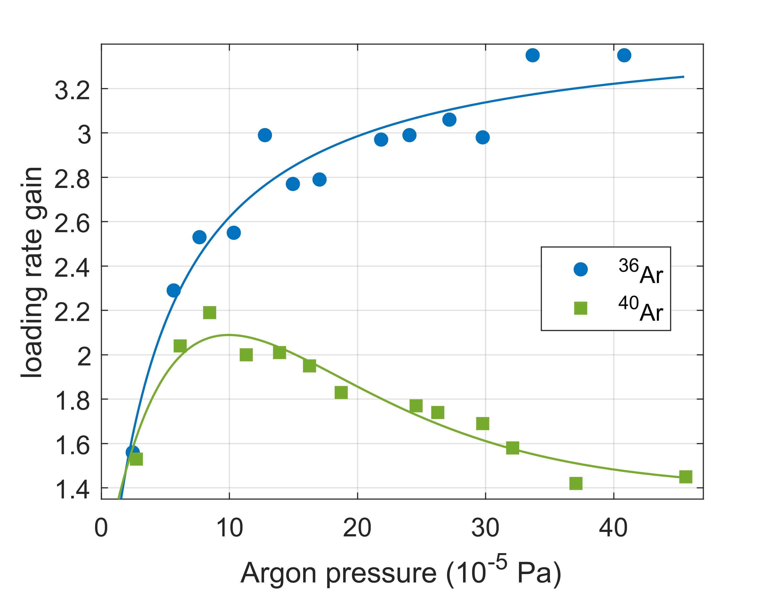
Figure 6: Loading rate gain vs argon pressure in the chamber at the outlet of the source tube (Fig. 2) for the 923-nm transition, measured with atmospheric argon. The pressure inside the source tube is considerably higher than at the outlet of the source tube. The lines are guides-to-the-eye.

The loading rate gains of the two isotopes differ significantly. For ³⁶Ar the loading rate gain increases with the argon pressure whereas for ⁴⁰Ar the loading rate gain decreases beyond a maximum. Moreover, the loading rate gain for ³⁶Ar in this measurement with atmospheric argon reaches the value 3.3 whereas it is only 2.2 when measured with the enriched sample (³⁶Ar abundance=$30\text{\,}\%$) as in Fig. 5. These findings indicate that the populations of the $1s$-levels in the discharge depend on pressure and composition. These dependences might be caused by various mechanisms such as trapping of light from the VUV ground level transitions, which together with the optical pumping light can produce metastable argon atoms.

IV Conclusion and Outlook

We have realized a two-fold increase of the ³⁹Ar loading rate in an atom trap system via optical pumping in the discharge source. A three-fold increase is expected by adding sidebands with additional laser power that cover all the hyperfine levels of ³⁹Ar. Similarly, we obtain an increase of the MOT loading rate by a factor 2-3 for the stable argon isotopes ³⁶Ar, ³⁸Ar and ⁴⁰Ar. We observe that the loading rate gain varies for different isotopes and that it depends on the argon pressure in the discharge as well as the abundance of the respective isotope. We assign these dependences to the complex population dynamics of the $1s$-levels in the discharge via mechanisms such as radiation trapping and metastable exchange collisions. Consequently, using the method presented here for practical ³⁹Ar analysis requires a stable control of the pressure so that the loading rate gain due to optical pumping for both ³⁹Ar and ³⁸Ar stays constant during measurements.
The hitherto unknown isotope shifts in ³⁶Ar and ³⁸Ar as well as the ³⁹Ar spectra for the 801-nm and 923-nm transitions have been measured in this work. They constitute an important contribution to the efforts on optically generating metastable argon via resonant two-photon excitation [35, 36]. For a more precise measurement of the hyperfine coefficients and the isotope shifts, spectroscopy on samples highly enriched in ³⁹Ar will be necessary [37, 38].
The presented method for enhanced production of metastable argon can be directly implemented in existing ATTA setups to increase the ³⁹Ar loading rate by a factor 2-3. For state-of-the-art ATTA systems, the ³⁹Ar loading rate is $\sim$$10\text{\,}\mathrm{a}\mathrm{t}\mathrm{o}\mathrm{m}\mathrm{s}\mathrm{/}\mathrm{h}$. For ³⁹Ar analysis at a precision level of $5\text{\,}\%$, this loading rate leads to a measuring time of $\sim$$50\text{\,}\mathrm{h}$ during which the ³⁹Ar background in the ATTA system increases linearly with time. Therefore, the two-fold increase in ³⁹Ar loading rate realized in this work constitutes a significant advance for measuring time, precision and sample size of ³⁹Ar analysis in environmental applications such as dating of alpine ice cores and large scale ocean surveys.

Appendix A Argon $1s-2p$ transitions

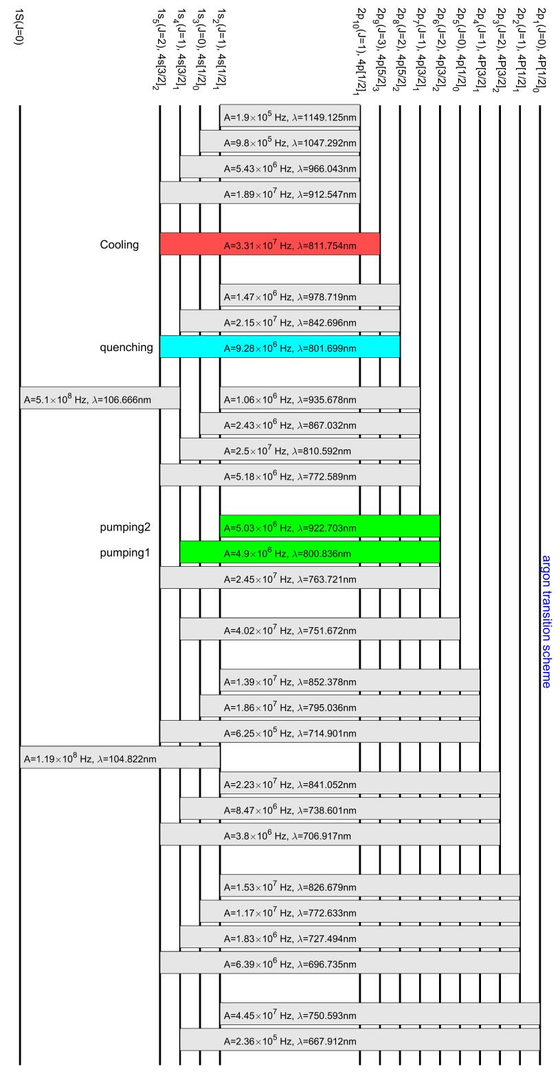
Figure 7: Argon transition scheme calculated based on [39] and adopted from [40, 41]. Levels with capital letter in the Racah notation refer to $j_{\text{core}}=1/2$ while levels with small letters refer to $j_{\text{core}}=3/2$.

Appendix B Master equation

The 6-level system for optical pumping of the even argon isotopes without hyperfine structures is illustrated in Fig. 1. As described in section I.1, $|1\rangle$ is the ground level and $|5\rangle$ the metastable level for laser cooling and trapping. Atoms in levels $|2\rangle$ and $|3\rangle$ can be transferred to $|5\rangle$ by driving the transition to $|4\rangle$ followed by spontaneous decay. $|6\rangle$ represents other levels that atoms can decay to from $|4\rangle$. Choosing the energy of level $|2\rangle$ as zero, $-\hbar\omega_{1},\hbar\omega_{3},\hbar\omega_{4},-\hbar\omega_{5}$ and $\hbar\omega_{6}$ are the energies of the corresponding levels relative to $|2\rangle$. In the interaction picture, the Hamiltonian of this atomic system interacting with the laser field is

$$\hat{H}=\hat{H}_{A}+\hat{H}_{AF},$$ (2)

where

$$\begin{split}\hat{H}_{A}&=\hbar\omega_{4}|4\rangle\langle 4|-\hbar\omega_{1}|1\rangle\langle 1|+\hbar\omega_{3}|3\rangle\langle 3|\\ &-\hbar\omega_{5}|5\rangle\langle 5|+\hbar\omega_{6}|6\rangle\langle 6|\end{split}$$ (3)

is the atomic Hamiltonian and

$$\begin{split}\hat{H}_{AF}&=&\frac{\hbar}{2}(\Omega_{24}^{*}\sigma_{24}e^{i\omega_{24}t}+\Omega_{24}\sigma_{42}e^{-i\omega_{24}t})\\ &&+\frac{\hbar}{2}(\Omega_{34}^{*}\sigma_{34}e^{i\omega_{34}t}+\Omega_{34}\sigma_{43}e^{-i\omega_{34}t})\end{split}$$ (4)

is the Hamiltonian that describes the interaction of the atoms with the light field. Here, $\omega_{24}$ and $\omega_{34}$ are the laser frequencies of the incident light, $\Omega_{24}$ and $\Omega_{34}$ are the corresponding Rabi frequencies and $\sigma_{ij}=|i\rangle\langle j|$ are the spin operators. With the unitary transformation $U=\mathrm{exp}(i\omega_{24}t|4\rangle\langle 4|+i(\omega_{24}-\omega_{34})t|3\rangle\langle 3|)$, the quantum level $|\psi\rangle$ changes to

$$\widetilde{|\psi\rangle}=U|\psi\rangle.$$ (5)

In this Schrödinger picture, the Hamiltonian becomes

$$\begin{split}\widetilde{H}&=UHU^{\dagger}+i\hbar(\partial_{t}U)U^{\dagger}\\ &=-\hbar\delta_{24}\sigma_{44}-\hbar\omega_{1}\sigma_{11}-\hbar\omega_{5}\sigma_{55}+\hbar\omega_{6}\sigma_{66}\\ &+\hbar(\delta_{34}-\delta_{24})\sigma_{33}+\frac{\hbar}{2}(\Omega_{24}\sigma_{42}+\Omega_{34}\sigma_{43}+h.c.)\\ \end{split}$$ (6)

where $\delta_{24}=\omega_{24}-\omega_{4}$ and $\delta_{34}=\omega_{34}-(\omega_{4}-\omega_{3})$ are the detunings of the light with respect to the transition frequencies.

The Lindblad master equation for the system including the spontaneous emission can be written as

$$\begin{split}\frac{d\widetilde{\rho}}{dt}&=\frac{1}{i\hbar}[\widetilde{H},\widetilde{\rho}]\\ &\quad+\Gamma_{42}(\sigma_{24}\widetilde{\rho}\sigma_{42}-\frac{1}{2}\widetilde{\rho}\sigma_{44}-\frac{1}{2}\sigma_{44}\widetilde{\rho})\\ &\quad+\Gamma_{21}(\sigma_{12}\widetilde{\rho}\sigma_{21}-\frac{1}{2}\widetilde{\rho}\sigma_{22}-\frac{1}{2}\sigma_{22}\widetilde{\rho})\\ &\quad+\Gamma_{45}(\sigma_{54}\widetilde{\rho}\sigma_{45}-\frac{1}{2}\widetilde{\rho}\sigma_{44}-\frac{1}{2}\sigma_{44}\widetilde{\rho})\\ &\quad+\Gamma_{46}(\sigma_{64}\widetilde{\rho}\sigma_{46}-\frac{1}{2}\widetilde{\rho}\sigma_{44}-\frac{1}{2}\sigma_{44}\widetilde{\rho})\\ &\quad+\Gamma_{43}(\sigma_{34}\widetilde{\rho}\sigma_{43}-\frac{1}{2}\widetilde{\rho}\sigma_{44}-\frac{1}{2}\sigma_{44}\widetilde{\rho})\\ &\quad+\Gamma_{31}(\sigma_{13}\widetilde{\rho}\sigma_{31}-\frac{1}{2}\widetilde{\rho}\sigma_{33}-\frac{1}{2}\sigma_{33}\widetilde{\rho})\\ \end{split}$$ (7)

where $\Gamma_{ij}$ is the spontaneous emission rate from $|i\rangle$ to $|j\rangle$. These equations describe the time evolution of $\widetilde{\rho}_{ij}=\langle i|\widetilde{\rho}|j\rangle$ and can be simplified to

$$\frac{d\widetilde{\rho}_{11}}{dt} =\Gamma_{21}\widetilde{\rho}_{22}+\Gamma_{31}\widetilde{\rho}_{33}$$

$$\frac{d\widetilde{\rho}_{22}}{dt} =\Gamma_{42}\widetilde{\rho}_{44}-\Gamma_{21}\widetilde{\rho}_{22}+\frac{i}{2}(\Omega_{24}\widetilde{\rho}_{24}-\Omega^{*}_{24}\widetilde{\rho}_{42})$$

$$\frac{d\widetilde{\rho}_{44}}{dt} =-(\Gamma_{42}+\Gamma_{45}+\Gamma_{46}+\Gamma_{43})\widetilde{\rho}_{44}$$

$$+\frac{i}{2}(\Omega^{*}_{24}\widetilde{\rho}_{42}-\Omega_{24}\widetilde{\rho}_{24})+\frac{i}{2}(\Omega^{*}_{34}\widetilde{\rho}_{43}-\Omega_{34}\widetilde{\rho}_{34})$$

$$\frac{d\widetilde{\rho}_{55}}{dt} =\Gamma_{45}\widetilde{\rho}_{44}$$

$$\frac{d\widetilde{\rho}_{66}}{dt} =\Gamma_{46}\widetilde{\rho}_{44}$$ (8)

$$\frac{d\widetilde{\rho}_{33}}{dt} =\Gamma_{43}\widetilde{\rho}_{44}-\Gamma_{31}\widetilde{\rho}_{33}+\frac{i}{2}(\Omega_{34}\widetilde{\rho}_{34}-\Omega^{*}_{34}\widetilde{\rho}_{43})$$

$$\frac{d\widetilde{\rho}_{42}}{dt} =-\frac{1}{2}(\Gamma_{42}+\Gamma_{21}+\Gamma_{45}+\Gamma_{46}+\Gamma_{43}-2i\delta_{24})\widetilde{\rho}_{42}$$

$$+\frac{i\Omega_{24}}{2}(\widetilde{\rho}_{44}-\widetilde{\rho}_{22})-\frac{i\Omega_{34}}{2}\widetilde{\rho}_{32}$$

$$\frac{d\widetilde{\rho}_{43}}{dt} =-\frac{1}{2}(\Gamma_{42}+\Gamma_{31}+\Gamma_{45}+\Gamma_{46}+\Gamma_{43}-2i\delta_{34})\widetilde{\rho}_{43}$$

$$+\frac{i\Omega_{34}}{2}(\widetilde{\rho}_{44}-\widetilde{\rho}_{33})-\frac{i\Omega_{24}}{2}\widetilde{\rho}_{23}$$

$$\frac{d\widetilde{\rho}_{32}}{dt} =-\frac{1}{2}(\Gamma_{21}+\Gamma_{31}+2i(\delta_{34}-\delta_{24}))\widetilde{\rho}_{32}$$

$$-\frac{i\Omega^{*}_{34}}{2}\widetilde{\rho}_{42}+\frac{i\Omega_{24}}{2}\widetilde{\rho}_{34}$$

Using that the population is initially in $|2\rangle$ and $|3\rangle$, i.e.

$$\begin{split}\widetilde{\rho}_{22}(t=0)&\neq 0\ ,\ \widetilde{\rho}_{33}(t=0)\neq 0\\ \widetilde{\rho}_{ij}(t=0)&=0,\text{ }(i,j)\not=(2,2),(i,j)\not=(3,3),\end{split}$$ (9)

then for the steady-state

$$\frac{d\widetilde{\rho}}{dt}(t\rightarrow+\infty)=0$$ (10)

Eq. B can be solved analytically using a computer algebra system, yielding the transfer efficiency $\widetilde{\rho}_{55}(t\to+\infty)$.

Appendix C TRANSFER EFFICIENCIES FOR $1s–2p$ TRANSITIONS IN ⁴⁰Ar

To determine the most suitable transitions for optical pumping to the metastable level $1s_{5}$, we have theoretically investigated all the $1s-2p$ transitions in argon. The transfer efficiency for each transition has been calculated according to the derivation in Sec. I.1 and the results are compiled in Table 3. For each $1s$ level we can thereby identify the transition with the highest transfer efficiency. Among these, we experimentally find the $1s_{2}-2p_{6}$ transition at $923\text{\,}\mathrm{n}\mathrm{m}$ and the $1s_{4}-2p_{6}$ transition at $801\text{\,}\mathrm{n}\mathrm{m}$ to be the strongest ones for optical pumping and therefore have chosen them for this work. A scheme of all $1s-2p$ transitions in argon is illustrated in Fig. 7 with the levels in Racah as well as in Paschen notation.

Table 3: Transfer efficiencies $\widetilde{\rho}_{55}(t\to+\infty)$ for $1s-2p$ transitions in ⁴⁰Ar calculated for a laser beam with 9-mm diameter and different powers $P$. The transitions highlighted in bold are the ones with the highest transfer efficiency. The levels are provided in Paschen as well as in Racah notation.

Lower level	Upper level	$\lambda\ $\text{\,}\mathrm{(}\mathrm{n}\mathrm{m}\mathrm{)}$$	Transfer efficiency $\widetilde{\rho}_{55}(t\to+\infty)$
			$P=$0.5\text{\,}\mathrm{W}$$	$P\rightarrow+\infty$\text{\,}\mathrm{W}$$
$1s_{4}$, $4s[3/2]_{1}$	$2p_{10}$, $4p[1/2]_{1}$	966.04	0.03	0.04
	$2p_{8}$, $4p[5/2]_{2}$	842.70	0.02	0.02
	$2p_{7}$, $4p[3/2]_{1}$	810.60	0.01	0.01
	$2p_{6}$, $4p[3/2]_{2}$	800.84	0.03	0.05
	$2p_{4}$, $4P[3/2]_{1}$	747.12	0.00	0.00
	$2p_{3}$, $4P[3/2]_{2}$	738.60	0.00	0.01
	$2p_{2}$, $4P[1/2]_{1}$	727.50	0.00	0.01
$1s_{3}$, $4s[1/2]_{0}$	$2p_{10}$, $4p[1/2]_{1}$	1047.30	0.77	0.77
	$2p_{7}$, $4p[3/2]_{1}$	867.03	0.17	0.17
	$2p_{4}$, $4P[3/2]_{1}$	795.04	0.04	0.04
	$2p_{3}$, $4P[1/2]_{1}$	772.63	0.27	0.27
$1s_{2}$, $4s[1/2]_{1}$	$2p_{10}$, $4p[1/2]_{1}$	1149.13	0.05	0.13
	$2p_{8}$, $4p[5/2]_{2}$	978.72	0.05	0.06
	$2p_{7}$, $4p[3/2]_{1}$	935.68	0.02	0.03
	$2p_{6}$, $4p[3/2]_{2}$	922.70	0.15	0.17
	$2p_{4}$, $4P[3/2]_{1}$	852.38	0.00	0.00
	$2p_{3}$, $4P[3/2]_{2}$	841.05	0.03	0.03
	$2p_{2}$, $4P[1/2]_{1}$	826.68	0.04	0.05

Appendix D ISOTOPE, HYPERFINE, AND TOTAL FREQUENCY SHIFTS FOR THE 801-nm AND 923-nm TRANSITION IN ³⁹Ar

Realizing optical pumping for the odd argon isotopes requires knowledge of the frequency shifts for the employed 801-nm and 923-nm transition. The total frequency shift is the sum of the isotope shift and the hyperfine shift. The isotope shifts for ³⁹Ar have not been measured and were calculated based on the measured isotope shifts for the stable isotopes (see Sec. I.2). The resulting isotope shifts for ³⁶Ar, ³⁸Ar and ³⁹Ar are shown in Table 4. The hyperfine constants of the involved levels have been measured for ³⁹Ar or can be calculated from measurements for ³⁷Ar (see Sec. I.2). The resulting hyperfine shifts for the different hyperfine levels are compiled in Table 6 together with the isotope shifts and the total frequency shifts.

Table 4: Isotope shifts relative to ⁴⁰Ar for the 801-nm and 923-nm transitions.

Transition nm	Isotope	Isotope shift MHz
801	36Ar	$-640(10)^{\text{a}}$
	38Ar	$-290(10)^{\text{a}}$
	39Ar	$-128(16)^{\text{b}}$
923	36Ar	$-960(10)^{\text{a}}$
	38Ar	$-445(10)^{\text{a}}$
	39Ar	$-202(16)^{\text{b}}$

• Measured in this work.

• Calculated in this work.

Table 5: Hyperfine coefficients $A$ and $B$ for ³⁹Ar and different levels.

Wavelength nm	level	$A$ MHz	B MHz
801	$1s_{4}$	$-334(2)^{\text{a}}$	$-24(3)^{\text{a}}$
	$2p_{6}$	$-163(31)^{\text{b}}$	$-63(11)^{\text{b}}$
923	$1s_{2}$	$-712(1)^{\text{a}}$	$84(6)^{\text{a}}$
	$2p_{6}$	$-163(31)^{\text{b}}$	$-63(11)^{\text{b}}$

• Reference [23].

• Reference [24].

Table 6: Isotope, hyperfine and total frequency shifts for the 801-nm and 923-nm transitions in ³⁹Ar. The hyperfine shift is relative to the center of gravity of the fine-structure term and the isotope shift is relative to ⁴⁰Ar.

Transition nm	Isotope shift MHz	Lower level $1s_{4}$/$1s_{2}$	Upper level $2p_{6}$	HFS shift MHz	Total shift MHz
801	$-128(16)$	$F=5/2$	$F=3/2$	-61(275)	-189(275)
			$F=5/2$	-440(198)	$-567(199)$
			$F=7/2$	$-985(92)$	$-1113(93)$
		$F=7/2$	$F=5/2$	701(198)	573 (199)
			$F=7/2$	155(92)	$27(93)$
			$F=9/2$	$-574(46)$	$-702(49)$
		$F=9/2$	$F=7/2$	1682(92)	1555(93)
			$F=9/2$	953(46)	826(49)
			$F=11/2$	$21(214)$	$-106(214)$
923	$-202(16)$	$F=5/2$	$F=3/2$	-1820(275)	-2022(275)
			$F=5/2$	$-2198(198)$	$-2401(199)$
			$F=7/2$	$-2744(92)$	$-2946(93)$
		$F=7/2$	$F=5/2$	400(198)	197(199)
			$F=7/2$	-146(92)	-348(93)
			$F=9/2$	$-875(46)$	$-1077(49)$
		$F=9/2$	$F=7/2$	2978(92)	2776(93)
			$F=9/2$	2249(46)	2047(49)
			$F=11/2$	$1317(214)$	$1115(214)$

References

- Stoenner et al. [1965] R. W. Stoenner, O. A. Schaeffer, and S. Katcoff, Science 148, 1325 (1965).
- Chen [2018] J. Chen, Nuclear Data Sheets 149, 1 (2018).
- Lal [1963] D. Lal, Earth Science and Meteorites 7, 115 (1963).
- Loosli and Oeschger [1968] H. H. Loosli and H. Oeschger, Earth and Planetary Science Letters 5, 191 (1968).
- Loosli [1983] H. Loosli, Earth and Planetary Science Letters 63, 51 (1983).
- Chen et al. [1999] C. Y. Chen, Y. M. Li, K. Bailey, T. P. O’Connor, L. Young, and Z.-T. Lu, Science 286, 1139 (1999).
- Jiang et al. [2012] W. Jiang, K. Bailey, Z.-T. Lu, P. Mueller, T. O’Connor, C.-F. Cheng, S.-M. Hu, R. Purtschert, N. Sturchio, Y. Sun, W. Williams, and G.-M. Yang, Geochimica et Cosmochimica Acta 91, 1 (2012).
- Lu et al. [2014] Z.-T. Lu, P. Schlosser, W. M. Smethie, N. C. Sturchio, T. P. Fischer, B. M. Kennedy, R. Purtschert, J. P. Severinghaus, D. K. Solomon, T. Tanhua, and R. Yokochi, Earth-Science Reviews 138, 196 (2014).
- Tian et al. [2019] L. Tian, F. Ritterbusch, J.-Q. Gu, S.-M. Hu, W. Jiang, Z.-T. Lu, D. Wang, and G.-M. Yang, Geophysical Research Letters 46, 6636 (2019).
- Jiang et al. [2011] W. Jiang, W. Williams, K. Bailey, A. M. Davis, S.-M. Hu, Z.-T. Lu, T. P. O’Connor, R. Purtschert, N. C. Sturchio, Y. R. Sun, and P. Mueller, Phys. Rev. Lett. 106, 103001 (2011).
- Ritterbusch et al. [2014] F. Ritterbusch, S. Ebser, J. Welte, T. Reichel, A. Kersting, R. Purtschert, W. Aeschbach-Hertig, and M. K. Oberthaler, Geophysical Research Letters 41, 6758 (2014).
- Ebser et al. [2018] S. Ebser, A. Kersting, T. Stöven, Z. Feng, L. Ringena, M. Schmidt, T. Tanhua, W. Aeschbach, and M. Oberthaler, Nature Communications 9 (2018).
- Feng et al. [2019] Z. Feng, P. Bohleber, S. Ebser, L. Ringena, M. Schmidt, A. Kersting, P. Hopkins, H. Hoffmann, A. Fischer, W. Aeschbach, and M. K. Oberthaler, Proceedings of the National Academy of Sciences 116, 8781 (2019).
- Tong et al. [2021] A. L. Tong, J.-Q. Gu, G.-M. Yang, S.-M. Hu, W. Jiang, Z.-T. Lu, and F. Ritterbusch, Review of Scientific Instruments 92, 063204 (2021).
- Gu et al. [2021] J.-Q. Gu, A. L. Tong, G.-M. Yang, S.-M. Hu, W. Jiang, Z.-T. Lu, R. Purtschert, and F. Ritterbusch, Chemical Geology 583, 120480 (2021).
- Paschen [1919] F. Paschen, Annalen der Physik 365, 405 (1919).
- Racah [1942] G. Racah, Physical Review 61, 537 (1942).
- Hans [2014] M. Hans, Bachelor thesis, Heidelberg University (2014).
- Frölian [2015] A. Frölian, Bachelor thesis, Heidelberg University (2015).
- Hickman et al. [2016] G. T. Hickman, J. D. Franson, and T. B. Pittman, Optics Letters 41, 4372 (2016).
- Lamsal et al. [2020] H. P. Lamsal, J. D. Franson, and T. B. Pittman, Optics Express 28, 24079 (2020).
- Zhang et al. [2020] Z.-Y. Zhang, F. Ritterbusch, W.-K. Hu, X.-Z. Dong, C. Y. Gao, W. Jiang, S.-Y. Liu, Z.-T. Lu, J. S. Wang, and G.-M. Yang, Phys. Rev. A 101, 053429 (2020).
- Traub et al. [1967] W. Traub, F. L. Roesler, M. M. Robertson, and V. W. Cohen, J. Opt. Soc. Am. 57, 1452 (1967).
- Klein et al. [1996] A. Klein, B. Brown, U. Georg, M. Keim, P. Lievens, R. Neugart, M. Neuroth, R. Silverans, L. Vermeeren, and ISOLDE Collaboration, Nuclear Physics A 607, 1 (1996).
- Armstrong [1971] L. Armstrong, Theory of the Hyperfine Structure of Free Atoms (Wiley-Interscience, New York, 1971) oCLC: 639161041.
- Stone [2015] N. J. Stone, Journal of Physical and Chemical Reference Data 44, 031215 (2015).
- King [1963] W. H. King, J. Opt. Soc. Am. 53, 638 (1963).
- Heilig and Steudel [1974] K. Heilig and A. Steudel, Atomic Data and Nuclear Data Tables Nuclear Charge and Moment Distributions, 14, 613 (1974).
- Cheng et al. [2013] C. F. Cheng, G. M. Yang, W. Jiang, Y. R. Sun, L. Y. Tu, and S. M. Hu, Optics Letters 38, 31 (2013).
- Zhao et al. [1998] W. Z. Zhao, J. E. Simsarian, L. A. Orozco, and G. D. Sprouse, Review of Scientific Instruments 69, 3737 (1998).
- Subhankar et al. [2019] S. Subhankar, A. Restelli, Y. Wang, S. L. Rolston, and J. V. Porto, Review of Scientific Instruments 90, 043115 (2019).
- Jia et al. [2020] Z. Jia, A. Tong, L. Sun, Y. Liu, J. Liu, Q. Wu, X. Fang, W. Yang, Y. Guo, F. Ritterbusch, Z.-T. Lu, W. Jiang, G. Yang, and Q. Chen, Review of Scientific Instruments 91, 033309 (2020).
- Tong et al. [2022] A. L. Tong, J.-Q. Gu, Z.-H. Jia, G.-M. Yang, S.-M. Hu, W. Jiang, Z.-T. Lu, F. Ritterbusch, and L.-T. Sun, Review of Scientific Instruments 93, 023203 (2022).
- Axner et al. [2004] O. Axner, J. Gustafsson, N. Omenetto, and J. D. Winefordner, Spectrochimica Acta Part B: Atomic Spectroscopy 59, 1 (2004).
- Wang et al. [2021] J. S. Wang, F. Ritterbusch, X.-Z. Dong, C. Gao, H. Li, W. Jiang, S.-Y. Liu, Z.-T. Lu, W.-H. Wang, G.-M. Yang, Y.-S. Zhang, and Z.-Y. Zhang, Phys. Rev. Lett. 127, 023201 (2021).
- Dong et al. [2022] X.-Z. Dong, F. Ritterbusch, D.-F. Yuan, J.-W. Yan, W.-T. Chen, W. Jiang, Z.-T. Lu, J. S. Wang, X.-A. Wang, and G.-M. Yang, Phys. Rev. A 105, L031101 (2022).
- Welte et al. [2009] J. Welte, I. Steinke, M. Henrich, F. Ritterbusch, M. K. Oberthaler, W. Aeschbach-Hertig, W. H. Schwarz, and M. Trieloff, Review of Scientific Instruments 80, 113109 (2009).
- Williams et al. [2011] W. Williams, Z.-T. Lu, K. Rudinger, C.-Y. Xu, R. Yokochi, and P. Mueller, Phys. Rev. A 83, 012512 (2011).
- Kramida et al. [2019] A. Kramida, Yu. Ralchenko, J. Reader, and NIST ASD Team, NIST Atomic Spectra Database (version 5.7.1), [Online]. Available: https://physics.nist.gov/asd [Apr 14 2020]. National Institute of Standards and Technology, Gaithersburg, MD. DOI: https://doi.org/10.18434/T4W30F (2019).
- Ritterbusch [2009] F. Ritterbusch, diploma thesis, Heidelberg University (2009).
- Welte [2011] J. Welte, PhD thesis, Heidelberg University (2011).