Universal trade-off structure between symmetry, irreversibility, and quantum coherence in quantum processes

Symmetry, irreversibility, and quantum coherence are foundational concepts in physics. Here, we present a universal trade-off relation that builds a bridge between these three concepts. This trade-off particularly reveals that (1) under a global symmetry, any attempt to induce local dynamics that change the conserved quantity will cause inevitable irreversibility, and (2) such irreversibility could be mitigated by quantum coherence. Our fundamental relation also admits broad applications in physics and quantum information processing. In the context of thermodynamics, we derive a trade-off relation between entropy production and quantum coherence in arbitrary isothermal processes. We also apply our relation to black hole physics and obtain a universal lower bound on how many bits of classical information thrown into a black hole become unreadable under the Hayden-Preskill model with the energy conservation law. This particularly shows that when the black hole is large enough, under suitable encoding, at least about $m/4$ bits of the thrown $m$ bits will be irrecoverable until 99 percent of the black hole evaporates. As an application to quantum information processing, we provide a lower bound on the coherence cost to implement an arbitrary quantum channel. We employ this bound to obtain a quantitative Wigner-Araki-Yanase theorem that comes with a clear operational meaning, as well as an error-coherence trade-off for unitary gate implementation and an error lower bound for approximate error correction with covariant encoding. Our main relation is based on quantum uncertainty relation, showcasing intimate connections between fundamental physical principles and ultimate operational capability.

I Introduction

Symmetry, irreversibility, and quantum superposition are foundational concepts in physics. In every field of physics, at least one of these three concepts plays a central role. First, symmetry is the dominant concept in modern physics. This concept describes the properties of a physical system that are invariant to specific operations. For example, a sphere has rotational symmetry because it remains unchanged by rotation. Symmetry can be formulated mathematically using the group theory and helps simplify many problems Georgi ; Hayashi . Furthermore, as Noether’s theorem predicts, imposing conservation laws, including the energy conservation law, is equivalent to requiring the corresponding symmetry Noether (1918). For this reason, any general physical theory that describes nature has some symmetry, allowing symmetry to be an effective guide to construct physical theories in modern physics Einstein (1916).

Irreversibility is another very successful concept. This concept appears in any situation where many-body effects involving a large number of particles are manifested. It plays a central role in thermodynamics Carnot (1824) and non-equilibrium physics Shiraishi et al. (2016) and limits the performance of various devices. As the second law of thermodynamics predicts, many thermodynamic processes are irreversible, which critically limits the performance of generators and engines Carnot (1824). Furthermore, quantum data and quantum resources, including entanglement, are not entirely recovered when damaged by thermal noise. Protecting quantum states from such irreversible changes is a central issue in the design of quantum devices Devitt et al. (2013).

Quantum superposition is a unique property of quantum mechanics describing that two different states can exist “superposed” simultaneously. It plays an essential role everywhere in quantum physics Sakurai and Napolitano (2011). Even in the technological sense, superposition has critical importance. In quantum information technology, it is a crucial resource for improving the performance of various devices. The use of quantum superposition to enhance the performance of devices such as computation Shor (1994); Grover (1996), communication Bennett and Wiesner (1992); Bennett and Brassard (2014), sensing Giovannetti et al. (2004, 2006), and engines Tajima and Funo (2021) has been studied actively in the last 30 years.

In this paper, we show that these three concepts are bonded together by quantum mechanical uncertainty relation Kennard (1927); Robertson (1929); Luo (2005a); Fröwis et al. (2015); Tajima and Nagaoka (2019). We establish a fundamental trade-off structure between the concepts. In this paper, we show that these three concepts are bonded together by a universal trade-off relation. The trade-off has two messages. First, under a global symmetry, if one tries to induce local dynamics that change the conserved quantity corresponding to the symmetry, the dynamics will be irreversible unless the change in the conserved quantity is simply a shift of the origin. Second, we can mitigate the irreversibility in proportional to the amount of coherence between the basis of the conserved quantity. Our trade-off holds for various irreversibility measures used in fields from stochastic thermodynamics to quantum information theory.

Since our trade-off theorem links the three fundamental concepts in physics, it has a wide range of applications (see Figure 2 for details). First, our theorem gives a lower bound on the required coherence to realize an arbitrary quantum process in a thermodynamic setup. This lower bound is provided as a function of the entropy production Funo et al. (2018), a standard measure of thermodynamic irreversibility. Since our result is derived from the quantum uncertainty relation, this result is an example of a direct restriction from the quantum uncertainty relation to thermodynamics. Our result is derived from the quantum uncertainty relation Kennard (1927); Robertson (1929); Luo (2005a); Fröwis et al. (2015); Tajima and Nagaoka (2019) and thus provides an example in which the uncertainty relation imposes a direct operational constraint in thermodynamical settings. This result can be further generalized to give the coherence cost of implementing any quantum channel in the standard-setting in the resource theory of asymmetry Marvian (2012); Zhang et al. (2017); Takagi (2019); Marvian (2020); Yamaguchi and Tajima (2022); Kudo and Tajima (2022); Ahmadi et al. (2013); Marvian and Spekkens (2012); Tajima and Nagaoka (2019); Tajima et al. (2018, 2020); Tajima and Saito (2021); Zhou et al. (2021); Yang et al. (2020); Liu and Zhou (2021a, b), which deals with symmetry.

Our theorem also provides a unified understanding of the relations between quantum information processing and symmetries. There are various known limitations that conservation laws and symmetries bring to quantum information processing. First, the Wigner-Araki-Yanase (WAY) theorem Wigner (1952); Araki and Yanase (1960) and its extensions Ozawa (2002a); Ahmadi et al. (2013); Marvian and Spekkens (2012); Tajima and Nagaoka (2019) state that under a conservation law, we cannot perform any error-free measurement of physical quantities that do not commute with a conserved quantity. It is also known that a similar theorem holds for general unitary dynamics Ozawa (2002b); Tajima et al. (2018, 2020); Tajima and Saito (2021). Also, for quantum error correction, the Eastin-Knill theorem Eastin and Knill (2009) and its extensions Faist et al. (2020); Kubica and Demkowicz-Dobrzański (2021); Zhou et al. (2021); Yang et al. (2020); Liu and Zhou (2021a, b); Tajima and Saito (2021) have shown that there can be no codes that implement all unitary gates from a continuous group with a transversal encoding. These theorems have been actively studied in recent years with various extensions. Our results can give all of these three theorems (WAY theorem, the unitary WAY theorem, and the Eastin-Knill theorem) and their quantitative extensions as corollaries. That is, the three theorems can be understood as particular aspects of the present trade-off theorem. Furthermore, our result provides new insights into this field. In particular, we extend the WAY theorem to give a trade-off between the fidelity error of measurement outputs and the coherence cost of the measurement. Although several quantitative versions of the WAY theorem have been given Ozawa (2002a); Ahmadi et al. (2013); Marvian and Spekkens (2012); Tajima and Nagaoka (2019); Korezekwa (2013), no bounds with a clear operational meaning, such as the fidelity error of the measurement output, have been obtained. Our extension of the WAY theorem corresponds to the solution to this open problem.

Our results further provide insights into black hole physics. There has been active research on how much Hawking radiation from a black hole must be collected to fully recover the information thrown into a black hole in the past decades. When there are no conservation laws in the black hole, the recovery can be made quickly Hayden and Preskill (2007). To recover a $k$-qubit system thrown into the black hole, we only have to collect $k$ and a few more qubits. In other words, Bob can read Alice’s diary, which was thrown into the black hole, via Hawking radiation. On the other hand, several studies have predicted a delay in this information recovery when the black hole observes the conservation of energy law Yoshida (2019); Liu (2020); Nakata et al. (2020); Tajima and Saito (2021). In particular, in Tajima and Saito (2021), a rigorous lower bound for the entanglement-fidelity-based recovery error was given, showing that the recovery error remains quite large until the large part of the black hole evaporates. These results suggest Bob will not read Alice’s diary under the energy conservation law to some extent. However, the question of how Alice’s diary becomes unreadable for Bob has still been unclear. The biggest problem is that the previous studies mainly evaluated the fidelity-based errors. The fidelity between two states becomes 0 even when only the states of a single qubit are orthogonal. Thus it is still unknown how many bits of Alice’s diary are unreadable to Bob. Our theorem allows us to overcome this problem. To be concrete, we can derive a lower bound on how many characters in Alice’s diary described in classical bits will be lost. As a rigorous theorem, we show that with a suitable coding, a bit-flip error occurs in at least about 1/4 of the $m$ bits of classical information thrown into the black hole. This error goes down as the black hole evaporates, but when the black hole is large enough, the bit-flip error remains close to $m/4$ bits until at least 99 percent of the black hole has evaporated.

Our results also apply to Petz map recoveries Hayden et al. (2004); Wilde (2015); Junge et al. (2018). Notably, all of the above applications, including thermodynamics, black holes, measurements, error-correcting codes, etc., are derived as direct corollaries from a single unification trade-off theorem.

II Framework

This paper aims to clarify how the irreversibility of quantum processes is affected by symmetry and coherence. To achieve this goal, we first introduce a framework for treating various types of the irreversibility of quantum processes simultaneously. As discussed later, our formulation is directly applicable to various topics, including quantum thermodynamics, quantum error correction, and black hole physics.

We consider two quantum systems, $A$ and $B$, represented in Figure 1. The system $A$ is the system of interest, and its initial state is not fixed. The system $B$ is another quantum system that works as an environment whose initial state is fixed to a quantum state $\rho_{B}$. We perform a unitary operation $U$ on $AB$ and divide $AB$ into two systems, $A^{\prime}$ and $B^{\prime}$. Then, the quantum process from $A$ to $A^{\prime}$ is described as a completely positive trace preserving (CPTP) map ${\cal E}(...):=\mathrm{Tr}_{B^{\prime}}[U...\otimes\rho_{B}U^{\dagger}]$. When $U$ has a global symmetry described by a Lie group, the symmetry provides conserved quantities via Noether’s theorem. For simplicity, we focus on a single conserved quantity $X$ under the unitary operation. Namely, we assume that

$$U^{\dagger}(X_{A^{\prime}}+X_{B^{\prime}})U=X_{A}+X_{B},$$ (1)

where $X_{\alpha}$ is the local operator of the conserved quantity on the system $\alpha$ ($\alpha=A,B,A^{\prime},B^{\prime}$).

Now, let us define the irreversibility of the quantum process ${\cal E}$. We prepare test states $\{\rho_{k}\}$ on $A$ with a probability $\{p_{k}\}$. We refer to the set $\{\rho_{k},p_{k}\}$ as test ensemble. The quantum process ${\cal E}$ changes the test states. After the process, we apply a CPTP map ${\cal R}$ on $A^{\prime}$, independent of $k$, and try to recover the test states of $A$ as accurately as possible. We then define the irreversibility of ${\cal E}$ for the test ensemble $\{\rho_{k},p_{k}\}$ as the average of the recovery error of the best recovery map as follows:

$$\delta :=\min_{{\cal R}:A^{\prime}\rightarrow A}\sqrt{\sum_{k}p_{k}\delta^{2}_{k}}$$ (2)

$$\delta_{k} :=D_{F}(\rho_{k},{\cal R}\circ{\cal E}(\rho_{k})).$$ (3)

Here $D_{F}$ is the purified distance defined as $D_{F}(\rho,\sigma):=\sqrt{1-F(\rho,\sigma)^{2}}$. The error $\delta$ includes various types of measures of irreversibility of ${\cal E}$ as special cases. For example, $\delta$ gives a lower bound for the entropy production, the standard measure of irreversibility in stochastic thermodynamics Funo et al. (2018). The irreversibility $\delta$ also includes the recovery error of the Petz recovery map Hayden et al. (2004); Wilde (2015); Junge et al. (2018) as a special case and gives a lower bound for the entanglement fidelity error Watrous (2018), a standard measure of irreversibility in quantum error correction and quantum information scrambling. For details, see the Methods section.

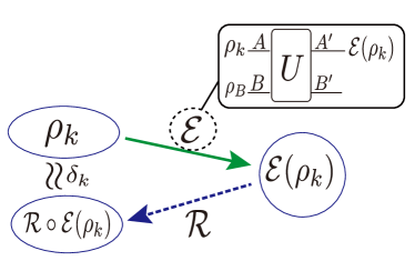
Figure 1: Schematic diagram of the framework. We prepare the test states $\{\rho_{k}\}$ with probability $\{p_{k}\}$ and perform a CPTP map ${\cal E}$ caused by a unitary interaction $U$. We try to recover the test states with a recovery CPTP map ${\cal R}$ independent of $k$, and define the irreversibility of ${\cal E}$ for the test ensemble $\{p_{k},\rho_{k}\}$ as the average of recovery error for the optimal recovery map: $\delta:=\sqrt{\sum_{k}p_{k}\delta^{2}_{k}}$. We investigate the restriction on the irreversibility under the assumption that $U$ satisfies the conservation law (1).

Next, we introduce a key quantity to describe the fundamental limitation of irreversibility. We first introduce a Hermitian operator corresponding to the change of the local conserved quantity caused by the quantum process ${\cal E}$:

$$Y:=X_{A}-{\cal E}^{\dagger}(X_{A^{\prime}}).$$ (4)

Here ${\cal E}^{\dagger}$ is the dual map of ${\cal E}$ that satisfies $\langle{\cal E}^{\dagger}(W)\rangle_{\rho}=\langle W\rangle_{{\cal E}(\rho)}$ for any $\rho$ and $W$. By definition, the expectation value of the change of the local conserved quantity caused by ${\cal E}$ is equal to the expectation value of $Y$. The key quantity is introduced as a kind of the summation of the non-diagonal elements of $Y$:

$${\cal C}:=\sqrt{\sum_{k\neq k^{\prime}}p_{k}p_{k^{\prime}}\mathrm{Tr}[(\rho_{k}-\rho_{k^{\prime}})_{+}Y(\rho_{k}-\rho_{k^{\prime}})_{-}Y]}.$$ (5)

Here $(\rho_{k}-\rho_{k^{\prime}})_{\pm}$ is the positive/negative part of $\rho_{k}-\rho_{k^{\prime}}$.

When the set of the test states are pure states $\{|\psi_{k}\rangle\}$ orthogonal to each other, ${\cal C}$ becomes the summation of the absolute values of the non-diagonal elements of $Y$: ${\cal C}=\sqrt{\sum_{k\neq k^{\prime}}p_{k}p_{k^{\prime}}|\langle\psi_{k}|Y|\psi_{k^{\prime}}\rangle|^{2}}$. The quantity ${\cal C}$ has a similar meaning even in the general case. The term $\mathrm{Tr}[(\rho_{k}-\rho_{k^{\prime}})_{+}Y(\rho_{k}-\rho_{k^{\prime}})_{-}Y]$ is non-negative, and it is non-zero if and only if $[Y,\Pi_{\pm}]\neq 0$, where $\Pi_{\pm}$ is the projection to the support of $(\rho_{k}-\rho_{k^{\prime}})_{\pm}$. Since the measurement $\{\Pi_{+},\Pi_{-}\}$ is the optimal measurement to distinguish $\rho_{k}$ and $\rho_{k^{\prime}}$, we can interpret $\mathrm{Tr}[(\rho_{k}-\rho_{k^{\prime}})_{+}Y(\rho_{k}-\rho_{k^{\prime}})_{-}Y]$ as the sum of the non-diagonal elements on the optimal basis to distinguish $\rho_{k}$ and $\rho_{k^{\prime}}$. In fact, $\mathrm{Tr}[(\rho_{k}-\rho_{k^{\prime}})_{+}Y(\rho_{k}-\rho_{k^{\prime}})_{-}Y]=\sum_{l,l^{\prime}}q_{l|+}q_{l^{\prime}|-}|\langle\phi_{l|+}|Y|\phi_{l^{\prime}|-}\rangle|^{2}$ holds where $\{q_{l|\pm}\}$ and $\{|\phi_{l|\pm}\rangle\}$ are the eigenvalues and eigenbasis of $(\rho_{k}-\rho_{k^{\prime}})_{\pm}$. Therefore, $\mathrm{Tr}[(\rho_{k}-\rho_{k^{\prime}})_{+}Y(\rho_{k}-\rho_{k^{\prime}})_{-}Y]$ is positive if and only if $Y$ has at least one non-diagonal element between an eigenvector of $(\rho_{k}-\rho_{k^{\prime}})_{+}$ and another eigenvector of $(\rho_{k}-\rho_{k^{\prime}})_{-}$.

As shown in the next section, the irreversibility $\delta$ is affected by quantum coherence about the conserved quantity. To analyze the coherence effect quantitatively, we introduce the SLD-quantum Fisher information Helstrom (1969); Holevo (2011) for the state family $\{e^{-iXt}\rho e^{iXt}\}_{t\in\mathbb{R}}$, which is a well-known measure of quantum coherence in the resource theory of asymmetry:

$${\cal F}_{\rho}(X):=4\lim_{\epsilon\rightarrow 0}\frac{D_{F}(e^{-iX\epsilon}\rho e^{iX\epsilon},\rho)}{\epsilon^{2}}$$ (6)

The quantum Fisher information is a good measure of quantum coherence on the eigenbasis of the conserved quantity $X$ Zhang et al. (2017); Marvian (2020); Takagi (2019); Yamaguchi and Tajima (2022); Kudo and Tajima (2022). It also quantifies the amount of the quantum fluctuation of $X$ Tóth and Petz (2013); Yu (2013); Luo (2005b); Hansen ; Marvian (2020); Kudo and Tajima (2022) (see the Methods section).

III Main Results

By using the quantities introduced in the previous section, we establish a general structure between symmetry, irreversibility, and coherence. To capture the essence, we first treat the case where the test states are orthogonal to each other, i.e., $F(\rho_{k},\rho_{k^{\prime}})=0$ for $k\neq k^{\prime}$. In this case, the following inequality holds:

$$\frac{{\cal C}}{\sqrt{{\cal F}}+\Delta}\leq\delta,$$ (7)

where ${\cal F}:={\cal F}_{\rho_{B}}(X_{B})$ is the quantum coherence in the initial state of $B$. When the test ensemble is in the form of $\{1/2,\rho_{k}\}_{k=1,2}$, we can make (7) tighter by substituting $\sqrt{2}{\cal C}$ for ${\cal C}$. And $\Delta$ is a positive quantity defined as

$$\Delta:=\max_{\rho\in\cup_{k}\mathrm{supp}(\rho_{k})}\sqrt{{\cal F}_{\rho\otimes\rho_{B}}(X_{A}\otimes 1_{B}-U^{\dagger}X_{A^{\prime}}\otimes 1_{B^{\prime}}U)}.$$ (8)

where the maximum runs over the subspace spanned by the supports of the test states $\{\rho_{k}\}$. We remark that $\Delta$ has several upper bounds, e.g., $\Delta\leq\Delta_{1}:=\Delta_{X_{A}}+\Delta_{X_{A^{\prime}}}$, where $\Delta_{W}$ is the difference between the maximum and minimum eigenvalues of $W$. Therefore, we can substitute these upper bounds for $\Delta$ in (7). For the details, see the Methods section.

The inequality (7) shows a close relationship between the global symmetry of dynamics $U$, the irreversibility of the process ${\cal E}$, and the quantum coherence in $B$. The message can be summarized in two points. First, it shows that when ${\cal C}$ is finite, the CPTP map ${\cal E}$ cannot be reversible. Note that unless $Y$ is proportional to the identity, i.e., unless the change of the local conserved quantity caused by ${\cal E}$ is just a shift of its origin, ${\cal C}>0$ holds at least one test ensemble. When $Y\not\propto I_{A}$, there are two eigenstates $|\psi_{0}\rangle$ and $|\psi_{1}\rangle$ of $Y$ with different eigenvalues, and we can easily see that ${\cal C}$ for the test states $\{|\psi_{\pm}\rangle:=(|\psi_{0}\rangle\pm|\psi_{1}\rangle)/\sqrt{2}\}$ is strictly greater than 0. Therefore, when local dynamics change the conserved quantity, the local dynamics will be irreversible unless the change of the local conserved quantity is just a shift of its origin.

Second, the irreversibility of ${\cal E}$ is mitigated by the quantum coherence in $B$. For example, when there is no quantum coherence in $B$, the irreversibility $\delta$ must be larger than ${\cal C}/\Delta$. On the other hand, when quantum coherence is present in the system $B$, the lower bound can be smaller than ${\cal C}/\Delta$. Thus, the equality (7) implies the suppression of irreversibility by coherence. These facts show that symmetry and coherence have opposite effects on irreversibility. While the global symmetry causes irreversibility, quantum coherence can mitigate the irreversibility.

The above trade-off structure also holds for the general case where the test states $\{\rho_{k}\}$ have no restriction. In the general case, the following inequality holds:

$$\frac{{\cal C}}{\sqrt{{\cal F}}+\Delta}\leq\sqrt{\delta}.$$ (9)

This inequality is quite similar to (7). The only difference is in the right hand side: $\delta$ in (7) changes to $\sqrt{\delta}$ in (9). Again, when the test ensemble is in the form of $\{1/2,\rho_{k}\}_{k=1,2}$, we can make (9) tighter by substituting $\sqrt{2}{\cal C}$ for ${\cal C}$. Clearly, (9) shows that the same structure as shown by (7) holds even if the test states have no restriction. When ${\cal C}$ is finite, the quantum process cannot be reversible. And the irreversibility can be alleviated by quantum coherence. The big difference between (7) and (9) is in their scopes of application. Unlike (7), inequality (9) does not impose any assumption on the test states. Therefore, (9) is applicable to various measures of irreversibility. Later, in Section IV and the Methods section, we will see that (9) provides general bounds for the entropy production of thermal operations and the recovery error of the Petz recovery map as examples.

We remark that the above results can be extended to the case where the conservation law (1) is violated. For this case, we define a Hermitian operator $Z$ that describes the degree of violation of the conservation as $Z:=U^{\dagger}(X_{A^{\prime}}+X_{B^{\prime}})U-(X_{A}+X_{B})$. Then, we can easily extend the inequalites (7) and (9) to this case by the following change:

$${\cal C}\rightarrow{\cal C}-\frac{\Delta_{Z}}{2}\enskip\mbox{and}\enskip\Delta\rightarrow\Delta+\Delta_{Z}.$$ (10)

The correction by (10) shows that when global symmetry is violated, our trade-off becomes weaker with the magnitude of the violation. In an extreme case where the global dynamics have no symmetry, $\Delta_{Z}$ becomes so large that ${\cal C}-\Delta_{Z}/2$ becomes negative, and our inequality becomes meaningless.

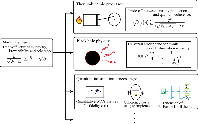
Figure 2: Schematic diagram of the logical relationship between the main results and applications. The arrow indicates that the tip is a corollary of the root. As shown in the figure, our results are applicable to black hole physics, quantum error-correcting codes, quantum measurements, gates implementations, and quantum thermodynamics. We remark that there are still more applications besides those depicted in this diagram. For example, we give a restriction on Petz map recovery, and coherence cost for arbitrary channels under thermodynamic setups.

Our results create a nexus between three fundamental concepts of physics: symmetry, irreversibility, and quantum superposition. As a result, our results apply to various topics in physics, including thermodynamic processes, black hole physics, measurements, gate implementations, quantum error-correcting codes, and Petz map recovery. (Figure 2). In the following three sections, we show the applications of our results in these fields. We remark that all of these applications are direct corollaries of the main results that are obtained by substituting proper ones for ${\cal E}$, $X$ and the test ensemble $\{p_{k},\rho_{k}\}$.

IV Application to thermodynamic processes

Our result (9) is directly applicable to thermodynamic processes. In thermodynamic settings, one often wants to interact heat reservoirs and batteries with a system to produce the desired dynamics ${\cal N}$ in the system. In such cases, the time evolution of the whole system is unitary and conserves energy. Therefore, our results can be used directly in this setup. For example, consider a three-body system containing a heat reservoir $R$, a target system $S$, and some battery $C$. The battery can be a work battery, a catalyst, or a combination of the two. At this point, by considering $X$ as Hamiltonian, $S$ as $A$, and $RC$ as $B$, we can apply (9) to this setup. Then, the quantum Fisher information of $X$ describes the amount of energetic coherence. Since the heat reservoir $R$ is in Gibbs state and has no energetic coherence, ${\cal F}^{\mathrm{cost}}_{{\cal N}}$ is the amount of coherence that $C$ should have. The restrictions given by (9) are general ones that hold no matter if $C$ is a catalyst, a work battery, or anything else. We remark that the discussion here is valid even for the case of multiple heat reservoirs, since each bath is in Gibbs state, which has no energetic coherence.

Based on the above discussion, we can derive two restrictions on thermodynamic processes from (9). First, we can link the amount of coherence in $C$ to the thermodynamic irreversibility of the realized channel ${\cal N}$, i.e., entropy production. When a CPTP map ${\cal N}$ does not change the Gibbs state at a specific inverse temperature $\beta$, then ${\cal N}$ is called a Gibbs preserving map. Here it is noteworthy that Gibbs preserving maps include all isothermal processes. The entropy production is defined as the following quantity for the Gibbs preserving map:

$$\Sigma_{\beta}(\rho):=\Delta S(\rho)-\beta Q(\rho)$$ (11)

Here, $\Delta S(\rho):=S({\cal N}(\rho))-S(\rho)$ and $Q(\rho):=\langle{\cal N}^{\dagger}(H)-H\rangle_{\rho}$ are the increases of the von-Neumann entropy and the energy of the target system. The entropy production corresponds to the total entropy increase in the target system and the bath after the total system is thermalized. As we see in the Methods section, the entropy production $\Sigma_{\beta}(\rho)$ is bounded from below by $\delta^{2}$ as $\Sigma_{\beta}(\rho)\geq 2\delta^{2}$, where $\delta$ is defined for the test ensemble $\{1/2,\rho_{k}\}_{k=1,2}$ where $\rho_{1}:=\rho$ and $\rho_{2}:=\rho_{\beta|H}$, here $\rho_{\beta|H}$ is the Gibbs state for the Hamiltonian $H$ and the inverse temperature $\beta$. In this case, since the test ensemble is in the form of $\{1/2,\rho_{k}\}_{k=1,2}$, we can use a tighter version of (9), whose ${\cal C}$ is substituted by $\sqrt{2}{\cal C}$. Therefore, from (9), we obtain the following trade-off relation between the entropy production and the coherence in $C$:

$$\sqrt{\Sigma_{\beta}(\rho)}\geq\frac{4{\cal C}^{2}}{(\sqrt{{\cal F}_{\rho_{C}}(X_{C})}+\Delta)^{2}}$$ (12)

The above trade-off is valid whenever the entropy production is well-defined, i.e., the process ${\cal N}$ is Gibbs preserving. Furthermore, we can obtain another restriction that is valid for an arbitrary process. When the process ${\cal N}$ is an arbitrary CPTP map, the entropy production is not well-defined in general, but we can define the generalized entropy production, another standard measure of irreversibility: $\Sigma_{{\cal N},\rho,\sigma}:=D(\rho\|\sigma)-D({\cal N}(\rho)\|{\cal N}(\sigma))$. When ${\cal N}$ is Gibbs preserving and $\sigma$ is the Gibbs state, $\Sigma_{{\cal N},\rho,\sigma}$ becomes $\Sigma_{\beta}(\rho)$. And as we see in the Methods section, the generalized entropy production is also bounded from below by $\delta^{2}$ as $\Sigma_{{\cal N},\rho,\sigma}\geq 2\delta^{2}$, where $\delta$ is defined for the test ensemble $\{1/2,\rho_{k}\}_{k=1,2}$ where $\rho_{1}:=\rho$ and $\rho_{2}:=\sigma$. Therefore, we can substitute $\Sigma_{{\cal N},\rho,\sigma}$ for $\Sigma_{\beta}(\rho)$ in (12). We remark that, in that case, (12) gives a universal lower bound for the coherence amount $C$ that is necessary to realize the given arbitrary channel ${\cal N}$:

$${\cal F}_{\rho_{C}}(X_{C})\geq\frac{4{\cal C}^{2}}{\sqrt{\Sigma_{{\cal N},\rho,\sigma}}}-\Delta^{2}.$$ (13)

V Application to Black hole physics

Our results also provide helpful insights into how the symmetry of black hole dynamics affects the recovery of information from black holes. To be concrete, we present a rigorous lower bound on how many of the $m$ bits of classical information string cannot be recovered in an information recovery protocol from a black hole with the energy conservation law.

We first review the background. In black hole physics, black holes and Hawking radiation from the black holes are often regarded as quantum many-body systems, and it has been analyzed how much information thrown into a black hole can be recovered from Hawking radiation. One of the pioneering studies is the Hayden-Preskill thought experiment Hayden and Preskill (2007). In the thought experiment, one considers the situation in which Alice throws a quantum system $A$ (her “diary” in the original paper) into a quantum black hole $B$ (Figure 3). And another person, Bob, tries to recover the diary’s contents from the Hawking radiation from the black hole. Then, we assume the following three basic assumptions. First, the black hole is old enough, and thus there is a quantum system $R_{B}$ corresponding to the early Hawking radiation that is maximally entangled with the black hole. To decode Alice’s diary contents, Bob can use not only the Hawking radiation $A^{\prime}$ after Alice throw her diary but also the early radiation $R_{B}$. Second, each system is described as qubits. We refer to the numbers of qubits of $A$, $A^{\prime}$, and $B$ as $k$, $l$, and $N$, respectively. Third, the dynamics of the black hole is the Haar random unitary $U$. These assumptions, especially the second and third, are pretty strong but widely accepted today.

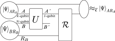
Figure 3: Schematic diagram of the Hayden-Preskill black hole model.

Under the above settings, Hayden and Preskill considered how long Bob should wait to see the contents of Alice’s diary. For the analysis, they considered a entanglement-fidelity based recovery error $\overline{\epsilon}$ defined as $\overline{\epsilon}:=\min_{{\cal R}_{A^{\prime}\rightarrow A}}D_{F}({\cal R}_{A^{\prime}\rightarrow A}\circ{\cal E}\otimes\mathrm{id}_{R}(\Psi),\Psi)$, where $\Psi$ is the maximally entangled state between $A$ and an external reference system $R_{A}$. And for the decoding error $\overline{\epsilon}$, they derived the following inequality:

$$\overline{\epsilon}\leq 2^{-(l-k)}.$$ (14)

The implication of this inequality was surprising: Bob hardly has to wait and can get the almost complete contents when the number of qubits in Hawking radiation $A^{\prime}$ was just a little more than the number of qubits in $A$.

The above result is derived via a rigorous argument once the setup is accepted. However, the above setup does not take conservation laws into account. Since the conservation law of energy for the whole system should be satisfied even for a black hole, it is necessary to consider the energy conservation law for a more accurate analysis. In recent years, analyses based on this idea have progressed, and it has been shown that taking energy conservation into account delays the escape of information from a black hole Yoshida (2019); Liu (2020); Nakata et al. (2020); Tajima and Saito (2021). These developments suggest that when the unitary $U$ is a Haar random unitary satisfying the energy conservation law, Bob may not read Alice’s diary to some extent under the energy conservation law. However, the question of how many classical bits in Alice’s diary become unreadable for Bob has not been analyzed due to two problems for the entanglement-fidelity-based errors that the previous studies evaluate. The first problem is in the fact that the fidelity between two states becomes 0 even when only the states of a single qubit are orthogonal. Thus the previous research does not allow us to determine how many bits of Alice’s diary are readable for Bob. The second problem is that the entanglement-fidelity-based analysis cannot assess the errors in the classical information encoded into specific quantum states.

Our result (7) allows us to overcome both of the above two problems. To be concrete, we can derive a lower bound on how many classical bits in Alice’s diary will be lost as a corollary of (7). For this purpose, let us introduce the error using the Hamming distance. We first introduce a classical $m$-bit string $\vec{a}:=(a_{1},...,a_{m})$. Here each $a_{j}$ takes values 0 or 1. To encode the classical string $\vec{a}$, we prepare the diary $A$ as a composite system of $m$ subsystems $A=A_{1}...A_{m}$, where each $A_{j}$ consists of $n$ qubits. Namely, $k=mn$ holds. We also prepare two pure states $|\psi^{(A_{j})}_{a_{j}}\rangle$ ($a_{j}=0,1$) on each subsystem $A_{j}$ which are orthogonal to each other. Using the pure states, we encode the string $\vec{a}$ into a pure state $|\psi_{\vec{a}}\rangle:=\otimes^{m}_{j=1}|\psi^{(A_{j})}_{a_{j}}\rangle$ on $A$. After the preparation, we throw the pure state $|\psi_{\vec{a}}\rangle$ into the black hole $B$. In other words, we perform the energy-preserving Haar random unitary $U$ on $AB$. After the unitary dynamics $U$, we try to recover the classical information $\vec{a}$. We perform a general measurement ${\cal M}$ on $A^{\prime}R_{B}$, and obtain a classical $m$-bit string $\vec{a}^{\prime}$ with probability $p^{\prime}_{\vec{a}}(\vec{a}^{\prime})$. We define the recovery error $\delta_{H}$ by averaging the Hamming distance between $\vec{a}$ and $\vec{a}^{\prime}$ for all possible input $\vec{a}$ as follows:

$$\delta_{H}:=\sum_{\vec{a},\vec{a}^{\prime}}\frac{p^{\prime}_{\vec{a}}(\vec{a}^{\prime})}{2^{m}}h(\vec{a},\vec{a}^{\prime}).$$ (15)

Here $h(\vec{a},\vec{a}^{\prime})$ is the Hamming distance, which represents the number of different bits between $\vec{a}$ and $\vec{a}^{\prime}$.

Let us show that by using proper states $\{|\psi^{A_{j}}_{a_{j}}\rangle\}$, we can make $\delta_{H}$ proportional to $m$. We assume that each qubit in $A$ has the same Hamiltonian $H:=|1\rangle\langle 1|$. Then, the energy eigenvalues of the Hamiltonian $H^{(A_{j})}$ on $A_{j}$ become integer from $0$ to $n$. We refer to the eigenvectors of $H^{A_{j}}$ with the eigenvalues $0$ and $n$ as $|0\rangle_{A_{j}}$ and $|n\rangle_{A_{j}}$, respectively, and define $|\psi^{A_{j}}_{0}\rangle:=(|0\rangle_{A_{j}}+|n\rangle_{A_{j}})/\sqrt{2}$ and $|\psi^{A_{j}}_{1}\rangle:=(|0\rangle_{A_{j}}-|n\rangle_{A_{j}})/\sqrt{2}$, respectively. Let us take $n:=a\sqrt{N}$, where $a$ is some positive constant satisfying $a\geq 2$. When $N\geq 10^{3}$ and $k\leq N$ holds, we obtain the following inequality from (7)

$$\delta_{H}\geq\frac{m}{4}\times\frac{1}{\left(1+\frac{3}{a\gamma}\right)^{2}},$$ (16)

where $\gamma:=1-\frac{l}{N+k}$ is the ratio between the number of qubits in the remained black hole $B^{\prime}$ and the total number of qubits $A^{\prime}B^{\prime}$.

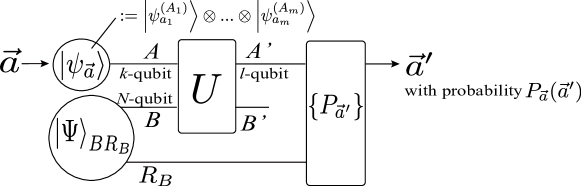
Figure 4: Schematic diagram of the classical information recovery in the Hayden-Preskill black hole model. We remark that $U$ satisfies $U^{\dagger}(X_{A^{\prime}}+X_{B^{\prime}})U=X_{A}+X_{B}$ and that $\vec{a}:=(a_{1},...,a_{m})$ and $k=m\times n$.

The inequality (16) is a lower bound on how many characters in Alice’s diary will be lost. We remark that this inequality holds for an arbitrary decoding method ${\cal M}$. Since the Hamming distance represents the number of bit-flip errors between the classical strings $\vec{a}$ and $\vec{a}^{\prime}$, the above inequality shows a lower bound of the average number of bit-flip errors in $m$-bit string given by $\gamma$. In other words, a non-negligible part of the classical bits cannot be read by Bob until most of the black hole has evaporated. We also stress that this inequality holds even when $k\ll N$ holds. Since $N$ corresponds to the Bekenstein-Hawking entropy of the black hole, $N$ is often a very large number. Then, $a\sqrt{N}$ can be much smaller than $N$, even if $a$ and $m$ are much larger than $1$. For example, the Bekenstein-Hawking entropy of Sagittarius A (the BH at the center of the Milky Way) is approximately equal to $10^{85}$ Almheiri et al. (2021). Therefore, if we set Sagittarius A as $B$, then $N=10^{85}$ holds. Let us set $a=10^{5}$ and $m=10^{7}$ ($m=10^{7}$ corresponds to the case that Alice hides 1 megabyte classical information in her dirary). Then, $k=ma\sqrt{N}=10^{54.5}$ and the inequality $k\ll N$ still holds. And in this case, the average bit-flip error in the classical data is approximately $m/4$ until 99 percent of the black hole evaporates.

VI Application to quantum information processing

As mentioned in Section 2, the quantum Fisher information is a widely used coherence measure. Our results, therefore, give universal lower bounds for the coherence cost to implement an arbitrary channel in a standard-setting in the resource theory of asymmetry Marvian (2012); Zhang et al. (2017); Takagi (2019); Marvian (2020); Yamaguchi and Tajima (2022); Kudo and Tajima (2022); Ahmadi et al. (2013); Marvian and Spekkens (2012); Tajima and Nagaoka (2019); Tajima et al. (2018, 2020); Tajima and Saito (2021); Zhou et al. (2021); Yang et al. (2020); Liu and Zhou (2021a, b). Let us define the implementation cost of an arbitrary CPTP map ${\cal N}$ from $A$ to $A^{\prime}$ as follows:

$${\cal F}^{\mathrm{cost}}_{{\cal N}}:=\min\{{\cal F}_{\rho_{B}}(X_{B})\enskip|\enskip(\rho_{B},X_{B},X_{B^{\prime}},U)\mbox{ realizes }{\cal N},\mbox{and satisfies \eqref{X-con}}\}.$$ (17)

Here, $(\rho_{B},X_{B},X_{B^{\prime}},U)$ is an implementation of ${\cal N}$ which satisfies ${\cal N}(...)=\mathrm{Tr}_{B^{\prime}}[U(...\otimes\rho_{B})U^{\dagger}]$ and $X_{A}+X_{B}=U^{\dagger}X_{A^{\prime}}+X_{B^{\prime}}U$. By definition, we can substitute ${\cal F}^{\mathrm{cost}}_{{\cal N}}$ for ${\cal F}$ in (7). Then, by setting the test ensemble arbitrary, these bounds give lower bounds for the cost ${\cal F}^{\mathrm{cost}}_{{\cal N}}$. For example, (7) gives the following bound for an arbitrary test ensemble satisfying $F(\rho_{k},\rho_{k^{\prime}})=0$ for $k\neq k^{\prime}$:

$$\sqrt{{\cal F}^{\mathrm{cost}}_{{\cal N}}}\geq\frac{{\cal C}}{\delta}-\Delta.$$ (18)

The obtained lower bound is applicable to arbitrary quantum channels, and thus they are very useful. In fact, it works as a unification theorem for various Wigner-Araki-Yanase type theorems for measurements, gate implementations, and error-correcting codes. Below, we will see several examples of the corollaries of (18) that shed new insights into each field.

Quantum measurement: a quantitative Wigner-Araki-Yanase theorem based on fidelity error— The relationship between quantum measurements and conservation laws has been actively studied for a long time Wigner (1952); Araki and Yanase (1960); Ozawa (2002a); Ahmadi et al. (2013); Marvian and Spekkens (2012); Tajima and Nagaoka (2019). In this field, one of the most important theorems is the Wigner-Araki-Yanase theorem, which states that under the existence of an (additive) conservation law, it is impossible to implement a projective measurement for a physical quantity that does not commute with the conserved quantity Wigner (1952); Araki and Yanase (1960).

The Wigner-Araki-Yanase theorem is a qualitative no-go theorem, and thus it is natural to consider quantitative variants of it Ozawa (2002a); Tajima and Nagaoka (2019). In these results, several trade-off relations between implementation error and cost of measurements have been given. Still, they measure the output error by the variance of a specific physical quantity called the noise operator, and the operational meaning of the error is not clear. The inequality (18) solves this problem and gives a quantitative Wigner-Araki-Yanase theorem for the fidelity error of the measurement outputs. Let ${\cal Q}$ and ${\cal P}$ be measurement channels from $A$ to $A^{\prime}$ defined as ${\cal Q}(...):=\sum_{k\in{\cal K}}\mathrm{Tr}[Q_{k}...]|k\rangle\langle k|$ and ${\cal P}(...):=\sum_{k\in{\cal K}}\mathrm{Tr}[P_{k}...]|k\rangle\langle k|$, where $\{Q_{k}\}$ and $\{P_{k}\}$ are PVM (projection valued measure) and POVM (positive operator valued measure) operators on $A$, respectively. We assume that $A^{\prime}$ is a classical memory system, and thus the conserved quantity $X_{A^{\prime}}$ on $A^{\prime}$ satisfies $[X_{A^{\prime}},|k\rangle\langle k|]=0$ (the Yanase condition Yanase (1961)). We assume that the projective measurement channel ${\cal Q}$ is approximated by ${\cal P}$, and define the fidelity-based approximation error as $\epsilon_{\mathrm{meas}}:=\max_{\rho}D_{F}({\cal P}(\rho),{\cal Q}(\rho))$. Then, (18) provides a lower bound for the implementation cost of ${\cal P}$ under conservation law of $X$ as follows:

$$\sqrt{{\cal F}^{\mathrm{cost}}_{{\cal P}}}\geq\max_{k}\frac{\sqrt{2}\|[X_{A},Q_{k}]\|_{\infty}}{\epsilon}-\Delta^{\prime}.$$ (19)

Here $\Delta^{\prime}:=\Delta_{X_{A}}+2\Delta_{X_{A^{\prime}}}$. We remark that when $X_{A^{\prime}}\propto I_{A^{\prime}}$ holds, $\Delta^{\prime}=\Delta_{X_{A}}$ also holds.

Gate implementations: trade-offs between coherence cost and implementation error– A similar theorem to the Wigner-Araki-Yanase theorem is known to hold for unitary gates Ozawa (2002b); Tajima et al. (2018, 2020); Tajima and Saito (2021). Under a conservation law, any attempt to implement an arbitrary unitary dynamics that does not commute with the conserved quantity will always result in a finite error Ozawa (2002b); Tajima et al. (2018, 2020); Tajima and Saito (2021); Tajima and Nagaoka (2019). And the amount of coherence that needs to be provided for implementation is inversely proportional to the implementation error Tajima et al. (2018, 2020); Tajima and Saito (2021). As we show in the supplementary materials, (18) reproduces these results as corollaries.

The inequality (18) also restricts the implementations of non-unitary gates. In fact, we can give the following no-go theorem: Let $U$ be a unitary and ${\cal N}$ be a channel. If there exist two orthogonal eigenstates $|x_{1,2}\rangle$ of $X$ such that $\langle{x_{1}|U^{\dagger}XU|x_{2}}\rangle\neq 0$ and ${\cal N}(|x_{1,2}\rangle\langle x_{1,2}|)=|x_{1,2}\rangle\langle x_{1,2}|$, then ${\cal E}={\cal N}\circ{\cal U}$ cannot be exactly implemented by a finite coherence resource state.

The above corollary is NOT a direct consequence of the no-go theorem for the implementation of coherent unitary. This is because the implementation of ${\cal E}={\cal N}\circ{\cal U}$ is not unique, and thus there are many other ways of realizing ${\cal E}$ other than sequentially implementing ${\cal U}$ and ${\cal N}$. The above result prohibits any such implementation of ${\cal E}$—the no-go theorem for the implementation of coherent unitary is rather a special case of the above corollary. Thus, this result extends the class of operations that do not allow for “resource state + free operation” implementation to that of non-unitary channels. For instance, a non-unitary example can be constructed by taking a coherent unitary $U$ and a dephasing channel ${\cal N}(\cdot)=\sum_{i}\Pi_{i}\cdot\Pi_{i}$, where $\Pi_{i}$ is the projection onto the subspace of charge $i$. The corresponding channel $\mathcal{E}=\mathcal{N}\circ\mathcal{U}$ is then a dephasing with respect to a rotated basis, and the above result ensures that such a dephasing cannot be implemented by any means with a finite coherent resource.

Quantum error corrections: An extension of Eastin-Knill theorem to classical information– There is a theorem similar to the WAY theorem in the field of quantum error correction. The Eastin-Knill theorem Eastin and Knill (2009) predicts that codes with the transversality for unitary operations which belong to a representation of a continuous group cannot make the decoding error zero. Recently, this theorem has been extended to quantitative theorems, which show that for covariant codes, the recovery error is inversely proportional to the number of the coding qubits Faist et al. (2020); Kubica and Demkowicz-Dobrzański (2021); Zhou et al. (2021); Yang et al. (2020); Liu and Zhou (2021a, b); Tajima and Saito (2021). As we show in the supplementary materials, the extended Eastin-Knill theorems can be derived from our result (18). Furthermore, we can extend the Eastin-Knill theorem to a restriction on the recovery of specific states. Let us consider a code channel ${\cal E}_{\mathrm{code}}$ from the “logical system” $L$ to the “physical system” $P$. We assume that the code ${\cal E}_{\mathrm{code}}$ is an isometry and covariant with respect to $\{U^{L}_{\theta}\}_{\theta\in\mathbb{R}}$ and $\{U^{P}_{\theta}\}_{\theta\in\mathbb{R}}$, where $U^{L}_{\theta}:=e^{i\theta X_{L}}$ and $U^{P}_{\theta}:=e^{i\theta X_{P}}$. The physical system $P$ is assumed to be a composite system of $N$ subsystems $\{P_{i}\}^{N}_{i=1}$, and the operator $X_{P}$ in $U^{P}_{\theta}$ is assumed to be written as $X_{P}=\sum_{i}X_{P_{i}}$. The noise ${\cal N}$ that occurs after the code channel ${\cal E}_{\mathrm{code}}$ is assumed to be the erasure noise, and the location of the noise is assumed to be known. Under this setup, we define the error of the channel ${\cal E}_{\mathrm{code}}$ for the noise ${\cal N}$ for a test ensemble $\{p_{k},\rho_{k}\}$ as follows:

$$\epsilon({\cal E}_{\mathrm{code}},{\cal N},\{p_{k},\rho_{k}\}):=\delta\mbox{ for the channel ${\cal R}\circ{\cal N}\circ{\cal E}_{\mathrm{code}}$ and the test ensemble $\{p_{k},\rho_{k}\}$}.$$ (20)

We remark that $\epsilon({\cal E}_{\mathrm{code}},{\cal N},\{p_{k},\rho_{k}\})$ is not the worst-case entanglement fidelity. It is defined as the fidelity error and it can describe the recovery error for arbitrary given ensemble $\{p_{k},\rho_{k}\}$ on $L$. Then, from (18), we can derive a universal lower bound for $\epsilon({\cal E}_{\mathrm{code}},{\cal N},\{p_{k},\rho_{k}\})$:

$$\epsilon({\cal E}_{\mathrm{code}},{\cal N},\{p_{k},\rho_{k}\})\geq\frac{{\cal C}}{\Delta}$$ (21)

From this bound, we can see to what extent the classical information encoded by the given ensemble is hurt. For example, we show that the following inequality holds for a specific $\{p_{k},\psi_{k}\}$:

$$\frac{\Delta_{X_{L}}}{\Delta_{X_{L}}+4\sqrt{2}N\max_{i}\Delta_{X_{P_{i}}}}\leq\epsilon({\cal E}_{\mathrm{code}},{\cal N},\{p_{k},\psi_{k}\}).$$ (22)

VII Summary

In this paper, we have given a universal trade-off structure between symmetry, irreversibility, and quantum coherence. This trade-off structure is quite general, applicable to measurements, gate implementations, error-correcting codes, thermodynamic processes, black holes, and Petz map recovery. These applications are obtained simply by substituting an appropriate test ensemble $\{p_{k},\rho_{k}\}$ and CPTP map ${\cal E}$ into the main theorem, yet they are very rich in content. First, as an application to thermodynamic processes, we derive a general trade-off between entropy production and coherence. As a further corollary, this gives a lower bound on the coherence cost of realizing an arbitrary channel in a thermodynamic setup.

Our theorem also provides new insight into black hole physics. We have shown that when a black hole satisfies the energy conservation, and when we throw $m$ bits of classical information encoded in an appropriate quantum state into the black hole, $m/4$ of the $m$ bits are damaged on average, no matter what recovery we perform. This damage decreases as the black hole evaporates, but if the black hole is large enough, we can ensure that the damage hardly reduces until 99 percent of the black hole has evaporated. It is important to emphasize that our results are valid even if the object thrown into the black hole is much smaller than the black hole.

Our theorem also provides a unified understanding and new contributions to the relationship between quantum information processings and symmetry. This field had several general restrictions, such as the Wigner-Araki-Yanase theorem and the Eastin-Knill theorem, each known as a separate theorem. Our theorem gives all of these as corollaries. In other words, we find that these restrictions are different aspects of a single unification theorem. We emphasize that our theorem reproduces not only previous results but also provides new limits. For example, a quantitative WAY theorem based on fidelity error has not been given before but can be given as a corollary from our theorem. Other restrictions on the degree to which classical information can be reconstructed with covariant codes can also be provided.

Our results and methods are expected to apply to various topics other than those presented here. We leave them as future work.

VIII Methods

VIII.1 Resource theory of asymmetry

For the readers’ convenience, we introduce the minimal tips for the resource theory of asymmetry and the quantum Fisher information briefly. The resource theory of asymmetry is a variant of resource theory Marvian (2012); Zhang et al. (2017); Takagi (2019); Marvian (2020); Yamaguchi and Tajima (2022); Kudo and Tajima (2022); Ahmadi et al. (2013); Marvian and Spekkens (2012); Tajima and Nagaoka (2019); Tajima et al. (2018, 2020); Tajima and Saito (2021); Zhou et al. (2021); Yang et al. (2020); Liu and Zhou (2021a, b) that handles symmetries and conservation laws. In the main text, we consider the case where the symmetry is described by the real number $\mathbb{R}$ or the unitary group $U(1)$. It is the simplest case where the dynamics have a single conserved quantity.

Like other resource theories, the resource theory of asymmetry has free states and free operations, called symmetric states and covariant operations. First, we define symmetric states. Let $\rho$ and $X_{S}$ be a state and a Hermitian operator of the conserved quantity on $S$. When $\rho$ satisfies the following relation, we call $\rho$ a symmetric state with respect to $\{e^{iX_{S}t}\}$.

$$e^{iX_{S}t}\rho e^{-iX_{S}t}=\rho,\enskip\forall t.$$ (23)

By definition, $\rho$ is symmetric with respect to $\{e^{iX_{S}t}\}$ if and only if $[\rho,X_{S}]=0$. In other words, a symmetric state is a quantum state with no coherence with respect to the eigenbasis of the conserved quantity.

Next, we define covariant operations. Let ${\cal E}_{S\rightarrow S^{\prime}}$ be a CPTP map from $S$ to $S^{\prime}$ and $X_{S}$ and $X_{S^{\prime}}$ be Hermitian operators on $S$ and $S^{\prime}$, respectively. When ${\cal E}_{S\rightarrow S^{\prime}}$ satisfies the following relation, we call ${\cal E}_{S\rightarrow S^{\prime}}$ a covariant operation with respect to $\{e^{iX_{S}t}\}$ and $\{e^{iX_{S^{\prime}}t}\}$:

$${\cal E}_{S\rightarrow S^{\prime}}(e^{iX_{S}t}...e^{-iX_{S}t})=e^{iX_{S^{\prime}}t}{\cal E}_{S\rightarrow S^{\prime}}(...)e^{-iX_{S^{\prime}}t},\enskip\forall t.$$ (24)

An important property of covariant operations is that we can realize an arbitrary covariant operation by using a proper unitary operation satisfying a conservation law and a quantum state which commutes with the conserved quantity. To be concrete, let ${\cal E}_{S\rightarrow S^{\prime}}$ be a covariant operation with respect to $\{e^{iX_{S}t}\}$ and $\{e^{iX_{S^{\prime}}t}\}$. Then, we can take quantum systems $E$ and $E^{\prime}$ satisfying $SE=S^{\prime}E^{\prime}$, Hermite operators $X_{E}$ and $X_{E^{\prime}}$ on $E$ and $E^{\prime}$, a unitary operation $U$ on $SE$ satisfying $U(X_{S}+X_{E})U^{\dagger}=X_{S^{\prime}}+X_{E^{\prime}}$, and a symmetric state $\mu_{E}$ on $E$ satisfying $[\mu_{E},X_{E}]=0$, and realize ${\cal E}_{S\rightarrow S^{\prime}}$ as follows Marvian (2020):

$${\cal E}_{S\rightarrow S^{\prime}}(...)=\mathrm{Tr}_{E^{\prime}}[U(...\otimes\mu_{E})U^{\dagger}].$$ (25)

The $SLD$-Fisher information for the family $\{e^{-iXt}\rho e^{iXt}\}_{t\in\mathbb{R}}$, described as ${\cal F}_{\rho_{S}}(X_{S})$, is known as a standard resource measure in the resource theory of asymmetry Takagi (2019); Marvian (2020); Yamaguchi and Tajima (2022). It is also a quantifier of quantum fluctuation, since it is related to the variance $V_{\rho_{S}}(X_{S}):=\langle X^{2}_{S}\rangle_{\rho_{S}}-\langle X_{S}\rangle^{2}_{\rho_{S}}$ as follows Tóth and Petz (2013); Yu (2013); Marvian (2020):

$${\cal F}_{\rho_{S}}(X_{S}) =4\min_{\{q_{i},\phi_{i}\}}\sum_{i}q_{i}V_{\phi_{i}}(X_{S}).$$ (26)

where $\{q_{i},\phi_{i}\}$ runs over the ensembles satisfying $\rho=\sum_{i}q_{i}\phi_{i}$ and each $\phi_{i}$ is pure. We remark that when $\rho$ is pure, ${\cal F}_{\rho}(X)=4V_{\rho}(X)$ holds. The equality (26) shows that ${\cal F}_{\rho}(X)$ is the minimum average of the fluctuation caused by quantum superposition. Therefore, we can interpret ${\cal F}_{\rho_{S}}(X_{S})$ as a quantum fluctuation of $X_{S}$.

VIII.2 Relation between $\delta$ and other irreversibility measures

In this subsection, we show that our irreversibility measure $\delta$ bounds other well-used irreversibility measures from below. This fact means that we can substitute the irreversibility measures for $\delta$ in our inequalities (7) and (9). Below we list the irreversibility measures bounded by $\delta$.

Irreversibility measures defined by entanglement fidelity: In quantum information theory, especially in the areas of quantum error corrections and gate implementations, entanglement fidelity-based recovery errors are often used. Three of the most commonly used recovery errors for a CPTP map ${\cal E}$ from $A$ to $A^{\prime}$ are as follows:

$$\epsilon_{\mathrm{worst}} :=\min_{{\cal R}_{A^{\prime}\rightarrow A}}\max_{\rho\mbox{ on }AR}D_{F}({\cal R}_{A^{\prime}\rightarrow A}\circ{\cal E}\otimes\mathrm{id}_{R}(\rho),\rho),$$ (27)

$$\overline{\epsilon} :=\min_{{\cal R}_{A^{\prime}\rightarrow A}}D_{F}({\cal R}_{A^{\prime}\rightarrow A}\circ{\cal E}\otimes\mathrm{id}_{R}(\Psi),\Psi),$$ (28)

$$\epsilon(\psi) :=\min_{{\cal R}_{A^{\prime}\rightarrow A}}D_{F}({\cal R}_{A^{\prime}\rightarrow A}\circ{\cal E}\otimes\mathrm{id}_{R}(\psi),\psi),$$ (29)

where $R$ is a reference system whose Hilbert space has the same dimension as that of $A$, $\Psi$ is the maximally entangled state on $AR$, and $\psi$ is an arbitrary pure state on $AR$. Clearly, $\overline{\epsilon}$ is a special case of $\epsilon(\psi)$. The irreversibility measure $\delta$ can provide lower bounds for these three errors.

First, for an arbitrary test ensemble $\{p_{k},\rho_{k}\}$, we obtain

$$\delta\leq\epsilon_{\mathrm{worst}}.$$ (30)

Second, for an arbitrary test ensemble $\{p_{k},\rho_{k}\}$ satisfying $\sum_{k}p_{k}\rho_{k}=I_{A}/d_{A}$ ($d_{A}$ is the dimension of $A$), we obtain

$$\delta\leq\overline{\epsilon}.$$ (31)

Third, for an arbitary pure state $\psi$ on $AR$ and for an arbitrary test ensemble $\{p_{k},\rho_{k}\}$ satisfying $\sum_{k}p_{k}\rho_{k}=\mathrm{Tr}_{R}[\psi]$, we obtain

$$\delta\leq\epsilon(\psi).$$ (32)

Petz map recovery: Our irreversibility measure $\delta$ also bounds the recovery error of the Petz recovery map. For an arbitrary quantum channel ${\cal N}$ and a “reference state” $\sigma$, the Petz recovery map is defined as follows Hayden et al. (2004):

$${\cal R}_{{\cal N},\sigma}(...):=\sqrt{\sigma}{\cal N}^{\dagger}(\sqrt{{\cal N}(\sigma)}^{-1}(...)\sqrt{{\cal N}(\sigma)}^{-1})\sqrt{\sigma}.$$ (33)

The Petz map introduced above has two important properties. First, the Petz map recovers the reference state perfectly, i.e., $\sigma={\cal R}_{{\cal N},\sigma}(\sigma)$. Second, the recovery error of the Petz map restricts the generalized entropy production $\Sigma_{{\cal N},\rho,\sigma}$. Let us define the recovery error of the Petz map as $\delta_{P}:=D_{F}(\rho,{\cal R}_{\sigma,{\cal N}}\circ{\cal N}(\rho))$. Then, the following inequality holds Wilde (2015); Junge et al. (2018):

$$\Sigma\geq-\log(1-\delta^{2}_{P})\geq\delta^{2}_{P}.$$ (34)

Due to these properties, the Petz map is widely used in various fields of quantum information science Barnum and Knill (2002) , statistical mechanics Alhambra and Woods (2017), and black hole physics Chen et al. (2020).

Now let us apply our theorem to the Petz recovery. Due to $\sigma={\cal R}_{{\cal N},\sigma}(\sigma)$, when we choose the channel ${\cal E}$ and the test ensemble $\{p_{k},\rho_{k}\}$ as ${\cal N}$ and $\{1/2,\rho_{k}\}_{k=1,2}$ where $\rho_{1}:=\rho$ and $\rho_{2}:=\sigma$, the irreversibility $\delta$ gives the following lower bound of the recovery error $\delta_{P}$ of the Petz map:

$$\delta\leq\min_{{\cal R}:\delta_{2}=0}\sqrt{\frac{\delta^{2}_{1}+\delta^{2}_{2}}{2}}\leq\frac{\delta_{P}}{\sqrt{2}}.$$ (35)

Therefore, (9) limits the error of Petz recovery $\delta_{P}$ directly.

Entropy production in thermodynamic processes, and its generalization: By combining (34) and (35), we obtain

$$2\delta^{2}\leq\Sigma.$$ (36)

And when a quantum channel ${\cal N}$ maps the Gibbs state with the temperature $\beta$ to the Gibbs state of the same temperature $\beta$, the generalized entropy production $\Sigma$ becomes the entropy production $\Sigma_{\beta}$ defined in (11). Therefore, when a quantum channel is Gibbs-preserving (i.e., when the entropy producition $\Sigma_{\beta}$ is well-defined), we obtain

$$2\delta^{2}\leq\Sigma_{\beta}.$$ (37)

VIII.3 Upper bounds $\Delta_{\alpha}$ of $\Delta$

The quantity $\Delta$ defined in (8) has several upper bounds:

$$\Delta \leq\Delta_{1}:=\Delta_{X_{A}}+\Delta_{X_{A^{\prime}}},$$ (38)

$$\Delta \leq\Delta_{2}:=\Delta_{Y}+2\sqrt{\|{\cal E}^{\dagger}(X^{2}_{A^{\prime}})-{\cal E}^{\dagger}(X_{A^{\prime}})^{2}\|_{\infty}}$$ (39)

$$\Delta \leq\Delta_{3}:=\max_{\rho\in\cup_{k}\mathrm{supp}(\rho_{k})}(\sqrt{{\cal F}_{\rho}(Y)}+\sqrt{{\cal F}_{\rho\otimes\rho_{B}}(U^{\dagger}X_{A^{\prime}}\otimes 1_{B^{\prime}}U-{\cal E}^{\dagger}(X_{A^{\prime}})\otimes 1_{B^{\prime}})}).$$ (40)

Due to the above three bounds, we can substitute $\Delta_{1}$, $\Delta_{2}$ and $\Delta_{3}$ for $\Delta$ in (7) and (9). When a statement, equation, etc., are valid using either $\Delta_{1}$, $\Delta_{2}$ or $\Delta_{3}$, we use the symbol $\Delta_{\alpha}$ to denote them collectively.

VIII.4 Shift invariance of ${\cal C}$, $\Delta$ and $\Delta_{\alpha}$

We also remark that ${\cal C}$, $\Delta$ and $\Delta_{\alpha}$ are invariant with respect to the shift of $X_{A}$ and $X_{A^{\prime}}$. To be concrete, when we define $\tilde{X}_{A}:=X_{A}+aI_{A}$, and $\tilde{X}_{A^{\prime}}:=X_{A^{\prime}}+bI_{A^{\prime}}$ where $a$ and $b$ are arbitrary real numbers, and when we also define $\tilde{{\cal C}}$, $\tilde{\Delta}$ and $\tilde{\Delta}_{\alpha}$ as ${\cal C}$, $\Delta$ and $\Delta_{\alpha}$ for $\tilde{X}_{A}$ and $\tilde{X}_{A^{\prime}}$, the following relations hold:

$$\tilde{{\cal C}}={\cal C},\enskip\tilde{\Delta}=\Delta,\enskip\tilde{\Delta}_{\alpha}=\Delta_{\alpha}.$$ (41)

VIII.5 Coherence cost of operator conversion

In this section, we introduce the method we use to derive the main results. The main results (7) and (9) are derived from a single lemma that rules the coherence cost of the operator conversion.

Lemma 1

Let us consider two quantum systems $S$ and $S^{\prime}$, and Hermitian operators $X_{S}$ and $X_{S^{\prime}}$ on them. We also take a projective operator $Q$ on $S$ and a non-negative operator $0\leq P\leq I$ on $S^{\prime}$. Let $\Lambda$ be a CPTP map from $S$ to $S^{\prime}$, and let its dual $\Lambda^{\dagger}$ approximately change $P$ to $Q$ as follows:

$$\langle\Lambda^{\dagger}(P)\rangle_{(1-Q)\rho_{S}(1-Q)}+\langle 1-\Lambda^{\dagger}(P)\rangle_{Q\rho_{S}Q}\leq\epsilon^{2}.$$ (42)

Here $\epsilon$ is a real positive number. We also introduce another quantum system $E$ and a tuple $(V,\rho_{E},X_{E},X_{E^{\prime}})$ of a unitary $V$ on $SE$, a state $\rho_{E}$ on $E$, an operator $X_{E}$ on $E$ and an operator $X_{E^{\prime}}$ on $E^{\prime}$, where $E^{\prime}$ is a quantum system satisfying $SE=S^{\prime}E^{\prime}$. We assume that $(V,\rho_{E},X_{E},X_{E^{\prime}})$ is an implementation of $\Lambda$ and satisfies the conservation law of $X$, i.e., $\Lambda(...)=\mathrm{Tr}_{E^{\prime}}[V(...\otimes\rho_{E})V^{\dagger}]$ and $X_{S}+X_{E}=V^{\dagger}(X_{S^{\prime}}+X_{E^{\prime}})V$. Then, the following relation holds:

$$\epsilon\geq\frac{|\langle[Q,Y_{S}]\rangle_{\rho_{S}}|}{\Delta_{S,S^{\prime},\rho_{S}}+\sqrt{{\cal F}_{\rho_{E}}(X_{E})}},$$ (43)

where $Y_{S}:=X_{S}-\Lambda^{\dagger}(X_{S^{\prime}})$ and $\Delta_{S,S^{\prime},\rho_{S}}$ is a symbol corresponding to $\Delta$, which is defined as

$$\Delta_{S,S^{\prime},\rho_{S}}:=\sqrt{{\cal F}_{\rho_{S}\otimes\rho_{E}}(X_{S}\otimes 1_{E}-V^{\dagger}X_{S^{\prime}}\otimes 1_{E^{\prime}}V)}.$$ (44)

The condition (42) means that if we perform measurements $\{Q,1-Q\}$ and $\{\Lambda^{\dagger}(P),1-\Lambda^{\dagger}(P)\}$ on $\rho_{S}$ in succession, the probability of a discrepancy between the results of the first and second measurements is less than $\epsilon$. In that sense, the number $\epsilon$ describes the error of the conversion from $P$ to $Q$ by $\Lambda^{\dagger}$ for the initial state $\rho_{S}$. And Lemma 1 says that to convert $P$ $\epsilon$-close to $Q$ in the sense of (43) holds, we need coherence ${\cal F}_{\rho_{E}}(X_{E})$ inversely proportional to $\epsilon^{2}$.

We can derive the main results (7) and (9) from Lemma 1 by choosing proper $P$, $Q$, and $\rho_{S}$ (for detail, see the supplementary materials). Furthermore, Lemma 1 is derived from the following improved version of the Kennard-Robertson uncertainty relation Fröwis et al. (2015); Tajima and Nagaoka (2019).

$$|\langle[O_{1},O_{2}]\rangle_{\rho}|\leq\sqrt{{\cal F}_{\rho}(O_{1})}\sqrt{V_{\rho}(O_{2})}.$$ (45)

In other words, all the main results and applications in this paper are derived from the quantum uncertainty relation.

I Derivation of Lemma 1

In this section, we derive Lemma 1 in the main text. For readers’ convenience, we repeat the lemma here:

Lemma 1

Let us consider two quantum systems $S$ and $S^{\prime}$, and Hermitian operators $X_{S}$ and $X_{S^{\prime}}$ on them. We also take a projective operator $Q$ on $S$ and a non-negative operator $P$ satisfying $0\leq P\leq I$ on $S^{\prime}$. Let $\Lambda$ be a CPTP map from $S$ to $S^{\prime}$, and let its dual $\Lambda^{\dagger}$ approximately change $P$ to $Q$ as follows:

$$\langle\Lambda^{\dagger}(P)\rangle_{(1-Q)\rho_{S}(1-Q)}+\langle 1-\Lambda^{\dagger}(P)\rangle_{Q\rho_{S}Q}\leq\epsilon^{2}.$$ (S.1)

Here $\epsilon$ is a real positive number, and $\Lambda^{\dagger}$ is the dual of $\Lambda$. We also introduce another quantum system $E$ and a tuple $(V,\rho_{E},X_{E},X_{E^{\prime}})$ of a unitary $V$ on $SE$, a state $\rho_{E}$ on $E$, an operator $X_{E}$ on $E$ and an operator $X_{E^{\prime}}$ on $E^{\prime}$, where $E^{\prime}$ is a quantum system satisfying $SE=S^{\prime}E^{\prime}$. We assume that $(V,\rho_{E},X_{E},X_{E^{\prime}})$ is an implementation of $\Lambda$ and satisfies the conservation law of $X$, i.e., $\Lambda(...)=\mathrm{Tr}_{E^{\prime}}[V(...\otimes\rho_{E})V^{\dagger}]$ and $X_{S}+X_{E}=V^{\dagger}(X_{S^{\prime}}+X_{E^{\prime}})V$. Then, the following relation holds:

$$\epsilon\geq\frac{|\langle[Q,Y_{S}]\rangle_{\rho_{S}}|}{\Delta_{S,S^{\prime},\rho_{S}}+\sqrt{{\cal F}_{\rho_{E}}(X_{E})}}.$$ (S.2)

where $Y_{S}:=X_{S}-\Lambda^{\dagger}(X_{S^{\prime}})$ and $\Delta_{S,S^{\prime},\rho_{S}}$ is a symbol corresponding to $\Delta$, which is defined as

$$\Delta_{S,S^{\prime},\rho_{S}}:=\sqrt{{\cal F}_{\rho_{S}\otimes\rho_{E}}(X_{S}\otimes 1_{E}-V^{\dagger}X_{S^{\prime}}\otimes 1_{E^{\prime}}V)}.$$ (S.3)

Proof: We first define the following operator:

$$N :=V^{\dagger}P\otimes 1_{E^{\prime}}V-Q\otimes 1_{E}.$$ (S.4)

Then, because of the improved Kennard-Robertson inequality (45), we obtain

$$|\langle[N,V^{\dagger}1_{S^{\prime}}\otimes X_{E^{\prime}}V]\rangle_{\rho_{S}\otimes\rho_{E}}|\leq\sqrt{{\cal F}_{\rho_{S}\otimes\rho_{E}}(V^{\dagger}1_{S^{\prime}}\otimes X_{E^{\prime}}V)}\sqrt{V_{\rho_{S}\otimes\rho_{E}}(N)}.$$ (S.5)

We evaluate $\sqrt{{\cal F}_{\rho_{S}\otimes\rho_{E}}(V^{\dagger}1_{S^{\prime}}\otimes X_{E^{\prime}}V)}$ as follows:

$$\sqrt{{\cal F}_{\rho_{S}\otimes\rho_{E}}(V^{\dagger}1_{S^{\prime}}\otimes X_{E^{\prime}}V)} \stackrel{{\scriptstyle(a)}}{{=}}\sqrt{{\cal F}_{\rho_{S}\otimes\rho_{E}}(-V^{\dagger}X_{S^{\prime}}\otimes 1_{E^{\prime}}V+X_{S}\otimes 1_{E}+1_{S}\otimes X_{E})}$$

$$\stackrel{{\scriptstyle(b)}}{{\leq}}\sqrt{{\cal F}_{\rho_{S}\otimes\rho_{E}}(X_{S}\otimes 1_{E}-V^{\dagger}X_{S^{\prime}}\otimes 1_{E^{\prime}}V)}+\sqrt{{\cal F}_{\rho_{S}\otimes\rho_{E}}(1_{S}\otimes X_{E})}$$

$$\stackrel{{\scriptstyle(c)}}{{=}}\sqrt{{\cal F}_{\rho_{S}\otimes\rho_{E}}(X_{S}\otimes 1_{E}-V^{\dagger}X_{S^{\prime}}\otimes 1_{E^{\prime}}V)}+\sqrt{{\cal F}_{\rho_{E}}(X_{E})}$$

$$=\Delta_{S,S^{\prime},\rho_{S}}+\sqrt{{\cal F}_{\rho_{E}}(X_{E})},$$ (S.6)

where we use the assumption $X_{S}+X_{E}=V^{\dagger}(X_{S^{\prime}}+X_{E^{\prime}})V$ by assumption in (a), the relation ${\cal F}_{\rho_{S}\otimes\rho_{E}}(X_{S}+X_{E})={\cal F}_{\rho_{S}}(X_{S})+{\cal F}_{\rho_{E}}(X_{E})$ Hansen in (c), and the inequality $\sqrt{{\cal F}_{\rho}(W+W^{\prime})}\leq\sqrt{{\cal F}_{\rho}(W)}+\sqrt{{\cal F}_{\rho}(W^{\prime})}$ which is shown as follows in (b):

$$\sqrt{{\cal F}_{\rho}(W+W^{\prime})} =\sqrt{\langle L_{W}+L_{W^{\prime}},L_{W}+L_{W^{\prime}}\rangle^{SLD}_{\rho}}$$

$$=\sqrt{\langle L_{W},L_{W}\rangle^{SLD}_{\rho}+\langle L_{W},L_{W^{\prime}}\rangle^{SLD}_{\rho}+\langle L_{W^{\prime}},L_{W}\rangle^{SLD}_{\rho}+\langle L_{W^{\prime}},L_{W^{\prime}}\rangle^{SLD}_{\rho}}$$

$$\leq\sqrt{\langle L_{W},L_{W}\rangle^{SLD}_{\rho}+2\sqrt{\langle L_{W},L_{W}\rangle^{SLD}_{\rho}\langle L_{W^{\prime}},L_{W^{\prime}}\rangle^{SLD}_{\rho}}+\langle L_{W^{\prime}},L_{W^{\prime}}\rangle^{SLD}_{\rho}}$$

$$=\sqrt{\langle L_{W},L_{W}\rangle^{SLD}_{\rho}}+\sqrt{\langle L_{W^{\prime}},L_{W^{\prime}}\rangle^{SLD}_{\rho}}$$

$$=\sqrt{{\cal F}_{\rho}(W)}+\sqrt{{\cal F}_{\rho}(W^{\prime})},$$ (S.7)

where $\langle O_{1},O_{2}\rangle^{SLD}_{\rho}:=\mathrm{Tr}[\rho(O_{1}O_{2}+O_{2}O_{1})/2]$ and $L_{O}$ is defined by $i[\rho,L_{O}]=(L_{O}\rho+\rho L_{O})/2$.

We also derive

$$V_{\rho_{S}\otimes\rho_{E}}(N) \leq\mathrm{Tr}[\rho_{S}\otimes\rho_{E}N^{2}]$$

$$=\mathrm{Tr}[\rho_{S}\otimes\rho_{E}(V^{\dagger}P^{2}\otimes 1_{E^{\prime}}V-V^{\dagger}P\otimes 1_{E^{\prime}}VQ\otimes 1_{E}-Q\otimes 1_{E}V^{\dagger}P\otimes 1_{E^{\prime}}V+Q\otimes 1_{E})]$$

$$\leq\mathrm{Tr}[\rho_{S}\otimes\rho_{E}(V^{\dagger}P\otimes 1_{E^{\prime}}V-V^{\dagger}P\otimes 1_{E^{\prime}}VQ\otimes 1_{E}-Q\otimes 1_{E}V^{\dagger}P\otimes 1_{E^{\prime}}V+Q\otimes 1_{E})]$$

$$=\mathrm{Tr}[\rho_{S}\otimes\rho_{E}((1_{S}-Q)\otimes 1_{E}V^{\dagger}P\otimes 1_{E^{\prime}}V(1_{S}-Q)\otimes 1_{E}+Q\otimes 1_{E}(1_{S}\otimes 1_{E}-V^{\dagger}P\otimes 1_{E^{\prime}}V)Q\otimes 1_{E})]$$

$$=\langle\Lambda^{\dagger}(P)\rangle_{(1-Q)\rho_{S}(1-Q)}+\langle\Lambda^{\dagger}(1-P)\rangle_{Q\rho_{S}Q}$$

$$\leq\delta^{2}$$ (S.8)

where in the second line we used that $Q^{2}=Q$ becasue $Q$ is a projective operator, in the third line we used $P^{2}\leq P$, and in the fifth line we used that for arbitrary positive semidefinite operators $A$ and $B$,

$$\langle\Lambda^{\dagger}(A)\rangle_{B\rho_{S}B} =\mathrm{Tr}[\Lambda^{\dagger}(A)B\rho_{S}B]$$ (S.9)

$$=\mathrm{Tr}[A\,\Lambda(B\rho_{S}B)]$$ (S.10)

$$=\mathrm{Tr}[A\,\mathrm{Tr}_{E}\left\{V(B\rho_{S}B\otimes\rho_{E})V^{\dagger}\right\}]$$ (S.11)

$$=\mathrm{Tr}[A\otimes 1_{E}V(B\rho_{S}B\otimes\rho_{E})V^{\dagger}]$$ (S.12)

$$=\mathrm{Tr}[\rho_{S}\otimes\rho_{E}B\otimes 1_{E}V^{\dagger}A\otimes 1_{E}VB\otimes 1_{E}].$$ (S.13)

We also transform the left-hand side of (S.5) as follows:

$$\langle[N,V^{\dagger}1_{S^{\prime}}\otimes X_{E^{\prime}}V]\rangle_{\rho_{S}\otimes\rho_{E}} =\langle[V^{\dagger}P\otimes 1_{E^{\prime}}V-Q\otimes 1_{E},V^{\dagger}(1_{S^{\prime}}\otimes X_{E^{\prime}})V]\rangle_{\rho_{S}\otimes\rho_{E}}$$

$$=-\langle[Q\otimes 1_{E},V^{\dagger}(1_{S^{\prime}}\otimes X_{E^{\prime}})V]\rangle_{\rho_{S}\otimes\rho_{E}}$$

$$=-\langle[Q\otimes 1_{E},X_{S}\otimes 1_{E}+1_{S}\otimes X_{E}-V^{\dagger}(X_{S^{\prime}}\otimes 1_{E^{\prime}})V]\rangle_{\rho_{S}\otimes\rho_{E}}$$

$$=-\langle[Q,Y_{S}]\rangle_{\rho_{S}}.$$ (S.14)

where in the third line we used the assumption $X_{S}+X_{E}=V^{\dagger}(X_{S^{\prime}}+X_{E^{\prime}})V$ and in the fourth line we used

$$\langle QY_{S}\rangle_{\rho_{S}} =\mathrm{Tr}[Q(X_{S}-\Lambda^{\dagger}(X_{S^{\prime}}))\rho_{S}]$$ (S.15)

$$=\mathrm{Tr}[Q\otimes 1_{E}(X_{S}\otimes 1_{E}-V^{\dagger}X_{S^{\prime}}\otimes 1_{E}V)\rho_{S}\otimes\rho_{E}]$$ (S.16)

and that $[Q\otimes 1_{E},1_{S}\otimes X_{E}]=0$. Hence, we obtain

$$|\langle[Q,Y_{S}]\rangle_{\rho_{S}}|\leq\delta\times(\Delta_{S,S^{\prime},\rho_{S}}+\sqrt{{\cal F}_{\rho_{E}}(X_{E})})$$ (S.17)

that we seek.

 

I.1 Extension to the case of violated conservation law

In Lemma 1, we assumed the conservation law $X_{S}+X_{E}=V^{\dagger}(X_{S^{\prime}}+X_{E^{\prime}})V$ holds. We can also treat the case where the conservation law is violated. Let us define a Hermitian operator $Z$ that describes the degree of violation of the conservation as $Z:=U^{\dagger}(X_{A^{\prime}}+X_{B^{\prime}})U-(X_{A}+X_{B})$. In this case, inequality (S.2) in Lemma 1 changes as follows:

$$\epsilon\geq\frac{|\langle[Q,Y_{S})]\rangle_{\rho_{S}}|-\frac{\Delta_{Z}}{2}}{\Delta_{S,S^{\prime},\rho_{S}}+\Delta_{Z}+\sqrt{{\cal F}_{\rho_{E}}(X_{E})}}.$$ (S.18)

where $\Delta_{Z}$ is the difference between the maximum and minimum eigenvalues of $Z$.

Proof: The proof is completely the same as the proof of (S.2) until (S.5):

$$|\langle[N,V^{\dagger}1_{S^{\prime}}\otimes X_{E^{\prime}}V]\rangle_{\rho_{S}\otimes\rho_{E}}|\leq\sqrt{{\cal F}_{\rho_{S}\otimes\rho_{E}}(V^{\dagger}1_{S^{\prime}}\otimes X_{E^{\prime}}V)}\sqrt{V_{\rho_{S}\otimes\rho_{E}}(N)}.$$ (S.19)

Since we do not use the conservation law in (S.8), we can use it again and obtain

$$|\langle[N,V^{\dagger}1_{S^{\prime}}\otimes X_{E^{\prime}}V]\rangle_{\rho_{S}\otimes\rho_{E}}|\leq\delta\sqrt{{\cal F}_{\rho_{S}\otimes\rho_{E}}(V^{\dagger}1_{S^{\prime}}\otimes X_{E^{\prime}}V)}.$$ (S.20)

We evaluate $\sqrt{{\cal F}_{\rho_{S}\otimes\rho_{E}}(V^{\dagger}1_{S^{\prime}}\otimes X_{E^{\prime}}V)}$ in the same manner as (S.6), but use $X_{S}+X_{E}+Z=V^{\dagger}(X_{S^{\prime}}+X_{E^{\prime}})V$ instead of $X_{S}+X_{E}=V^{\dagger}(X_{S^{\prime}}+X_{E^{\prime}})V$:

$$\sqrt{{\cal F}_{\rho_{S}\otimes\rho_{E}}(V^{\dagger}1_{S^{\prime}}\otimes X_{E^{\prime}}V)} =\sqrt{{\cal F}_{\rho_{S}\otimes\rho_{E}}(-V^{\dagger}X_{S^{\prime}}\otimes 1_{E^{\prime}}V+X_{S}\otimes 1_{E}+1_{S}\otimes X_{E}+Z)}$$

$$\leq\sqrt{{\cal F}_{\rho_{S}\otimes\rho_{E}}(X_{S}\otimes 1_{E}-V^{\dagger}X_{S^{\prime}}\otimes 1_{E^{\prime}}V)}+\sqrt{{\cal F}_{\rho_{S}\otimes\rho_{E}}(1_{S}\otimes X_{E})}+\sqrt{{\cal F}_{\rho_{S}\otimes\rho_{E}}(Z)}$$

$$=\sqrt{{\cal F}_{\rho_{S}\otimes\rho_{E}}(X_{S}\otimes 1_{E}-V^{\dagger}X_{S^{\prime}}\otimes 1_{E^{\prime}}V)}+\sqrt{{\cal F}_{\rho_{E}}(X_{E})}+\sqrt{{\cal F}_{\rho_{S}\otimes\rho_{E}}(Z)}$$ (S.21)

Therefore, we obtain

$$\sqrt{{\cal F}_{\rho_{S}\otimes\rho_{E}}(V^{\dagger}1_{S^{\prime}}\otimes X_{E^{\prime}}V)}\leq\sqrt{{\cal F}_{\rho_{E}}(X_{E})}+\Delta_{Z}+\Delta_{S,S^{\prime},\rho_{S}}.$$ (S.22)

Similarly, we evaluate $|\langle[N,V^{\dagger}1_{S^{\prime}}\otimes X_{E^{\prime}}V]\rangle_{\rho_{S}\otimes\rho_{E}}|$ in the same manner as (S.14) but use $X_{S}+X_{E}+Z=V^{\dagger}(X_{S^{\prime}}+X_{E^{\prime}})V$ instead of $X_{S}+X_{E}=V^{\dagger}(X_{S^{\prime}}+X_{E^{\prime}})V$:

$$\langle[N,V^{\dagger}1_{S^{\prime}}\otimes X_{E^{\prime}}V]\rangle_{\rho_{S}\otimes\rho_{E}} =-\langle[Q\otimes 1_{E},V^{\dagger}(1_{S^{\prime}}\otimes X_{E^{\prime}})V]\rangle_{\rho_{S}\otimes\rho_{E}}$$

$$=-\langle[Q\otimes 1_{E},X_{S}\otimes 1_{E}+1_{S}\otimes X_{E}-V^{\dagger}(X_{S^{\prime}}\otimes 1_{E^{\prime}})V+Z]\rangle_{\rho_{S}\otimes\rho_{E}}$$

$$=-\langle[Q,Y_{S}]\rangle_{\rho_{S}}-\langle[Q\otimes 1_{E},Z]\rangle_{\rho_{S}\otimes\rho_{E}}.$$ (S.23)

Therefore, we obtain

$$|\langle[N,V^{\dagger}1_{S^{\prime}}\otimes X_{E^{\prime}}V]\rangle_{\rho_{S}\otimes\rho_{E}}| \geq|\langle[Q,Y_{S}]\rangle_{\rho_{S}}|-|\langle[Q\otimes 1_{E},Z]\rangle_{\rho_{S}\otimes\rho_{E}}|$$

$$\geq\langle[Q,Y_{S}]\rangle_{\rho_{S}}|-\sqrt{{\cal F}_{\rho_{S}\otimes\rho_{E}}(Q\otimes 1_{E})}\sqrt{V_{\rho_{S}\otimes\rho_{E}}(Z)}$$

$$\stackrel{{\scriptstyle(a)}}{{\geq}}\langle[Q,Y_{S}]\rangle_{\rho_{S}}|-\frac{\Delta_{Z}}{2}.$$ (S.24)

Here we use ${\cal F}_{\rho_{S}\otimes\rho_{E}}(Q\otimes 1_{E})\leq 1$ due to $0\leq Q\leq 1$ and $V_{\rho_{S}\otimes\rho_{E}}(Z)\leq\frac{\Delta^{2}_{Z}}{4}$.

Combining the above, we obtain (S.18).   

II Derivation of (7) and (9)

In this section, we derive (7) and (9) in the main text from Lemma 1. To this end, we prove the following theorem that includes (7) and (9) as special cases:

Theorem 1

Let us consider two quantum systems $A$ and $A^{\prime}$, and Hermitian operators $X_{A}$ and $X_{A^{\prime}}$ on them. Let ${\cal E}$ be a CPTP map from $A$ to $A^{\prime}$ which is implemented by unitary interaction with another system $B$ that satisfies the conservation law of $X$. To be concrete, we introduce a tuple $(U,\rho_{B},X_{B},X_{B^{\prime}})$ of a unitary $U$ on $AB$, a state $\rho_{B}$ on $B$, an operator $X_{B}$ on $B$ and an operator $X_{B^{\prime}}$ on $B^{\prime}$, where $B^{\prime}$ is a quantum system satisfying $AB=A^{\prime}B^{\prime}$, and assume that

$${\cal E}(...)=\mathrm{Tr}_{B^{\prime}}[U(...\otimes\rho_{B})U^{\dagger}],\enskip X_{A}+X_{B}=U^{\dagger}(X_{A^{\prime}}+X_{B^{\prime}})U.$$ (S.25)

We also take a test ensemble $\{p_{k},\rho_{k}\}$ where $\{\rho_{k}\}$ is a set of quantum states and $\{p_{k}\}$ is a probability distribution. We define two measures of irreversibility of ${\cal E}$ for the test ensemble $\{p_{k},\rho_{k}\}$ as

$$\delta:=\sqrt{\sum_{k}p_{k}\delta^{2}_{k}},\enskip\delta_{T}:=\sum_{k}p_{k}\delta_{k,T},$$ (S.26)

where $\delta_{k}:=D_{F}(\rho_{k},{\cal R}\circ{\cal E}(\rho_{k}))$ and $\delta_{k,T}:=T(\rho_{k},{\cal R}\circ{\cal E}(\rho_{k}))$ where $T(\rho,\sigma):=\|\rho-\sigma\|_{1}/2$. Then, for arbitrary $\{\rho_{k},p_{k}\}$, the following relation holds:

$$\frac{{\cal C}}{\Delta+\sqrt{{\cal F}_{\rho_{E}}(X_{E})}}\leq\sqrt{\delta_{\mathrm{multi}}}$$ (S.27)

Here, we can substitute either the following $\delta_{\mathrm{multi1}}$ or $\delta_{\mathrm{multi2}}$ for $\delta_{\mathrm{multi}}$:

$$\delta_{\mathrm{multi1}} :=\delta\times\overline{T}$$ (S.28)

$$\delta_{\mathrm{multi2}} :=\delta_{T}\times\left(1-\min_{k}p_{k}\right),$$ (S.29)

where $\overline{T}:=\sqrt{\sum_{k,k^{\prime}}p_{k}p_{k^{\prime}}T(\rho_{k},\rho_{k^{\prime}})^{2}}\leq 1$ and

$${\cal C}:=\sqrt{\sum_{k\neq k^{\prime}}p_{k}p_{k^{\prime}}\mathrm{Tr}[(\rho_{k}-\rho_{k^{\prime}})_{+}Y(\rho_{k}-\rho_{k^{\prime}})_{-}Y]}.$$ (S.30)

where $(\rho_{k}-\rho_{k^{\prime}})_{\pm}$ is the positive/negative part of $\rho_{k}-\rho_{k^{\prime}}$, and $Y:=X_{A}-{\cal E}^{\dagger}(X_{A^{\prime}})$. And $\Delta$ is defined as

$$\Delta:=\max_{\rho\in\cup_{k}\mathrm{supp}(\rho_{k})}\sqrt{{\cal F}_{\rho\otimes\rho_{B}}(X_{A}\otimes 1_{B}-U^{\dagger}X_{A^{\prime}}\otimes 1_{B^{\prime}}U)},$$ (S.31)

where the minimum runs over the subspace which is the sum of the supports the test states $\{\rho_{k}\}$. Furthermore, when $\{\rho_{k}\}$ are orthogonal to each other, i.e., when $F(\rho_{k},\rho_{k^{\prime}})=0$ for any $k\neq k^{\prime}$,

$$\frac{{\cal C}}{\Delta+\sqrt{{\cal F}_{\rho_{E}}(X_{E})}}\leq\delta\times\sqrt{1-\min_{k}p_{k}}.$$ (S.32)

Clearly, (9) and (7) are direct corollaries of (S.27) and (S.32) due to $\overline{T}\leq 1$ and $1-\min_{k}p_{k}\leq 1$. We also remark that when the test ensemble $\{p_{k},\rho_{k}\}_{k\in{\cal K}}$ satisfies ${\cal K}=\{0,1\}$ and $p_{k}=1/2$, then $\sqrt{1-\min_{k}p_{k}}=\sqrt{1/2}$. Therefore, for an arbitrary test ensemble in the form of $\{1/2,\rho_{k}\}_{k=1,2}$, the bound (S.32) becomes stronger than (7) by $\sqrt{2}$.

We prove (S.27) and (S.32) separately. We first prove (S.32).

Proof of (S.32):   We show (S.32) under the assumption that $\{\rho_{k}\}$ are orthogonal to each other. Note that we can take a projective measurement $\{Q_{k}\}$ that completely distinguishes $\{\rho_{k}\}$ in this case, i.e., $\mathrm{Tr}[Q_{k}\rho_{k}]=1$. We define a CPTP map ${\cal Q}(...):=\mathrm{Tr}[Q_{k}...]|k\rangle\langle k|_{S}$. Then, by the monotonicity of $D_{F}$, we obtain

$$\delta_{k}\geq D_{F}({\cal Q}(\rho_{k}),{\cal Q}\circ{\cal R}\circ{\cal E}(\rho_{k})).$$ (S.33)

The above implies

$$\mathrm{Tr}[{\cal E}^{\dagger}\circ{\cal R}^{\dagger}(Q_{k})\rho_{k}] \geq 1-\delta^{2}_{k},$$ (S.34)

$$\mathrm{Tr}[{\cal E}^{\dagger}\circ{\cal R}^{\dagger}(Q_{k^{\prime}})\rho_{k}]\leq\mathrm{Tr}[(1-{\cal E}^{\dagger}\circ{\cal R}^{\dagger}(Q_{k}))\rho_{k}] \leq\delta^{2}_{k}\enskip(k\neq k^{\prime}).$$ (S.35)

Now, let us take a spectral decompotion of $\rho_{k}$ as $\rho_{k}=\sum_{l}q^{(k)}_{l}\psi^{(k)}_{l}$, and define

$$1-\delta^{2}_{(k),l}:=\mathrm{Tr}[{\cal E}^{\dagger}\circ{\cal R}^{\dagger}(Q_{k})\psi^{(k)}_{l}],$$ (S.36)

$$\delta^{2}_{(k),[k^{\prime}],l}:=\mathrm{Tr}[{\cal E}^{\dagger}\circ{\cal R}^{\dagger}(Q_{k^{\prime}})\psi^{(k)}_{l}].$$ (S.37)

Then, due to (S.34) and (S.35),

$$\sum_{l}q^{(k)}_{l}\delta^{2}_{(k),l} \leq\delta^{2}_{k},$$ (S.38)

$$\sum_{l}q^{(k)}_{l}\delta^{2}_{(k),[k^{\prime}],l} \leq\delta^{2}_{k},\enskip\forall k^{\prime}\mbox{ s.t. }k^{\prime}\neq k.$$ (S.39)

Let us define $\rho^{k,k^{\prime},l,l^{\prime},\theta}_{A}$ as

$$\rho^{k,k^{\prime},l,l^{\prime},\theta}_{A}:=\left(\frac{|\psi^{(k)}_{l}\rangle+e^{i\theta}|\psi^{(k^{\prime})}_{l^{\prime}}\rangle}{\sqrt{2}}\right)\left(\frac{\langle\psi^{(k)}_{l}|+e^{-i\theta}\langle\psi^{(k^{\prime})}_{l^{\prime}}|}{\sqrt{2}}\right),$$ (S.40)

for $\theta\in\mathbb{R}$. Note that $\rho^{k,k^{\prime},l,l^{\prime},\theta}_{A}$ for $k\neq k^{\prime}$ satisfies

$$Q_{k}\rho^{k,k^{\prime},l,l^{\prime},\theta}_{A}Q_{k} =\frac{\psi^{(k)}_{l}}{2},$$ (S.41)

$$(1-Q_{k})\rho^{k,k^{\prime},l,l^{\prime},\theta}_{A}(1-Q_{k}) =\frac{\psi^{(k^{\prime})}_{l^{\prime}}}{2}.$$ (S.42)

Therefore, $\rho^{k,k^{\prime},l,l^{\prime},\theta}_{A}$ and $P_{k}:={\cal R}^{\dagger}(Q_{k})$ satisfy

$$\mathrm{Tr}[(1-{\cal E}^{\dagger}(P_{k}))Q_{k}\rho^{k,k^{\prime},l,l^{\prime},\theta}_{A}Q_{k}]+\mathrm{Tr}[{\cal E}^{\dagger}(P_{k})(1-Q_{k})\rho^{k,k^{\prime},l,l^{\prime},\theta}_{A}(1-Q_{k})] =\frac{\mathrm{Tr}[(1-{\cal E}^{\dagger}\circ{\cal R}^{\dagger}(Q_{k}))\psi^{(k)}_{l}]+\mathrm{Tr}[{\cal E}^{\dagger}\circ{\cal R}^{\dagger}(Q_{k})\psi^{(k^{\prime})}_{l^{\prime}}]}{2}$$

$$=\frac{\delta^{2}_{(k),l}+\delta^{2}_{(k^{\prime}),[k],l^{\prime}}}{2}.$$ (S.43)

Combining Lemma 1 and (S.43), we obtain

$$\frac{\delta^{2}_{(k),l}+\delta^{2}_{(k^{\prime}),[k],l^{\prime}}}{2} \geq\frac{|\langle[Q_{k},Y_{A}]\rangle_{\rho^{k,k^{\prime},l,l^{\prime},\theta}_{A}}|^{2}}{(\sqrt{{\cal F}_{\rho^{k,k^{\prime},l,l^{\prime},\theta}_{A}\otimes\rho_{B}}(X_{A}\otimes 1_{B}-V^{\dagger}X_{A^{\prime}}\otimes 1_{B^{\prime}}V)}+\sqrt{{\cal F}_{\rho_{B}}(X_{B})})^{2}}$$

$$\stackrel{{\scriptstyle(a)}}{{\geq}}\frac{|\langle[Q_{k},Y_{A}]\rangle_{\rho^{k,k^{\prime},l,l^{\prime},\theta}_{A}}|^{2}}{(\max_{\rho\in\cup_{k}\mathrm{supp}(\rho_{k})}\sqrt{{\cal F}_{\rho\otimes\rho_{B}}(X_{A}\otimes 1_{B}-U^{\dagger}X_{A^{\prime}}\otimes 1_{B^{\prime}}U)}+\sqrt{{\cal F}_{\rho_{B}}(X_{B})})^{2}}$$

$$=\frac{|\langle[Q_{k},Y_{A}]\rangle_{\rho^{k,k^{\prime},l,l^{\prime},\theta}_{A}}|^{2}}{(\Delta+\sqrt{{\cal F}_{\rho_{B}}(X_{B})})^{2}}$$ (S.44)

Here, we use $\psi_{k,k^{\prime},l,l^{\prime},\theta}=\rho^{k,k^{\prime},l,l^{\prime},\theta}_{A}$ in (a), which is valid under the present condition, since $(\rho_{k}-\rho_{k^{\prime}})_{+}=\rho_{k}$ and $(\rho_{k}-\rho_{k^{\prime}})_{-}=\rho_{k^{\prime}}$ hold when $F(\rho_{k},\rho_{k^{\prime}})=0$. We evaluate $\langle[Q_{k},Y_{A}]\rangle_{\rho^{k,k^{\prime},l,l^{\prime},\theta}_{A}}$ as

$$\langle[Q_{k},Y_{A}]\rangle_{\rho^{k,k^{\prime},l,l^{\prime},\theta}_{A}}=\frac{e^{i\theta}\langle\psi^{(k)}_{l}|Y_{A}|\psi^{(k^{\prime})}_{l^{\prime}}\rangle-(c.c)}{2}.$$ (S.45)

Therefore, by defining $e^{i\eta}:=\frac{\langle\psi^{(k)}_{l}|Y_{A}|\psi^{(k^{\prime})}_{l^{\prime}}\rangle}{|\langle\psi^{(k)}_{l}|Y_{A}|\psi^{(k^{\prime})}_{l^{\prime}}\rangle|}$ and taking $\theta:=\frac{\pi}{2}-\eta$, we obtain

$$\langle[Q_{k},Y_{A}]\rangle_{\rho^{k,k^{\prime},l,l^{\prime},\theta}_{A}}=i|\langle\psi^{(k)}_{l}|Y_{A}|\psi^{(k^{\prime})}_{l^{\prime}}\rangle|.$$ (S.46)

Therefore,

$$\frac{\delta^{2}_{(k),l}+\delta^{2}_{(k^{\prime}),[k],l^{\prime}}}{2} \geq\frac{|\langle\psi^{(k)}_{l}|Y_{A}|\psi^{(k^{\prime})}_{l^{\prime}}\rangle|^{2}}{(\Delta+\sqrt{{\cal F}_{\rho_{B}}(X_{B})})^{2}}$$ (S.47)

Multiplying by $p_{k}p_{k^{\prime}}q^{(k)}_{l}q^{(k^{\prime})}_{l^{\prime}}$, summing for $l$ and $l^{\prime}$, and summing for $k$ and $k^{\prime}$ with $k\neq k^{\prime}$, we obtain (S.32) as follows:

$$\frac{{\cal C}^{2}}{(\Delta+\sqrt{{\cal F}_{\rho_{B}}(X_{B})})^{2}} =\sum_{k\neq k^{\prime}}\sum_{l,l^{\prime}}p_{k}p_{k^{\prime}}q^{(k)}_{l}q^{(k^{\prime})}_{l^{\prime}}\frac{|\langle\psi^{(k)}_{l}|Y_{A}|\psi^{(k^{\prime})}_{l^{\prime}}\rangle|^{2}}{(\Delta+\sqrt{{\cal F}_{\rho_{B}}(X_{B})})^{2}}$$

$$\leq\sum_{k\neq k^{\prime}}\sum_{l,l^{\prime}}p_{k}p_{k^{\prime}}q^{(k)}_{l}q^{(k^{\prime})}_{l^{\prime}}\frac{\delta^{2}_{(k),l}+\delta^{2}_{(k^{\prime}),[k],l^{\prime}}}{2}$$

$$\leq\sum_{k\neq k^{\prime}}\sum_{l^{\prime}}p_{k}p_{k^{\prime}}q^{(k^{\prime})}_{l^{\prime}}\frac{\delta^{2}_{k}}{2}+\sum_{k\neq k^{\prime}}\sum_{l}p_{k}p_{k^{\prime}}q^{(k)}_{l}\frac{\delta^{2}_{k^{\prime}}}{2}$$

$$=\sum_{k\neq k^{\prime}}p_{k}p_{k^{\prime}}\frac{\delta^{2}_{k}}{2}+\sum_{k\neq k^{\prime}}p_{k}p_{k^{\prime}}\frac{\delta^{2}_{k^{\prime}}}{2}$$

$$=\sum_{k}p_{k}(1-p_{k})\delta^{2}_{k}\leq\left(1-\min_{k}p_{k}\right)\times\delta^{2}.$$ (S.48)

 

To prove (S.27), we use the following lemma:

Lemma 2

Let us consider a quantum system $S$ and two states $\rho_{0}$ and $\rho_{1}$ on it. We suppose that a POVM $\{P,1-P\}$ and a real positive number $\delta$ satisfy

$$\frac{1}{2}\|p_{0}-p_{1}\|_{1}\approx_{\delta}\frac{1}{2}\|\rho_{0}-\rho_{1}\|_{1},$$ (S.49)

where $x\approx_{\delta}y\stackrel{{\scriptstyle\mathrm{def.}}}{{\Leftrightarrow}}|x-y|\leq\delta$, $p_{0}$ and $p_{1}$ are probability distributions that are defined as $p_{j}(+):=\mathrm{Tr}[\rho_{j}P]$ and $p_{j}(-):=\mathrm{Tr}[\rho_{j}(1-P)]$, and $\|p_{0}-p_{1}\|_{1}:=|p_{0}(+)-p_{1}(+)|+|p_{0}(-)-p_{1}(-)|$. Suppose that $P$ is taken so that $p_{0}(+)\geq p_{1}(+)$. Then, the following inequality holds:

$$\mathrm{Tr}[(1-P)(\rho_{0}-\rho_{1})_{+}]+\mathrm{Tr}[P(\rho_{0}-\rho_{1})_{-}]\leq\delta.$$ (S.50)

Proof of Lemma 2:   We first note the following:

$$|p_{0}(+)-p_{1}(+)| =\frac{1}{2}\|p_{0}-p_{1}\|_{1}$$

$$\approx_{\delta}\frac{1}{2}\|\rho_{0}-\rho_{1}\|_{1}$$

$$=\mathrm{Tr}[(\rho_{0}-\rho_{1})_{+}].$$ (S.51)

Therefore, because of the definition $\{p_{j}(+)\}_{j=0,1}$, we obtin

$$\mathrm{Tr}[(\rho_{0}-\rho_{1})_{+}]\approx_{\delta}|\mathrm{Tr}[P(\rho_{0}-\rho_{1})]|.$$ (S.52)

Then, we obtain

$$\mathrm{Tr}[(\rho_{0}-\rho_{1})_{+}]-\delta \leq|\mathrm{Tr}[P(\rho_{0}-\rho_{1})]|$$

$$=\mathrm{Tr}[P(\rho_{0}-\rho_{1})_{+}]-\mathrm{Tr}[P(\rho_{0}-\rho_{1})_{-}].$$ (S.53)

This is equivalent to the desired inequality (S.50).   

Now, let us prove (S.27).

Proof of (S.27):   Due to the definition of $\delta_{k}$ $\delta_{k,T}$, the triangle inequality and the monotonicity of the trace norm, we obtain

$$\frac{1}{2}\|\rho_{k}-\rho_{k^{\prime}}\|_{1} \leq\frac{1}{2}\|\rho_{k}-{\cal R}\circ{\cal E}(\rho_{k})\|_{1}+\|{\cal R}\circ{\cal E}(\rho_{k})-{\cal R}\circ{\cal E}(\rho_{k^{\prime}})\|_{1}+\frac{1}{2}\|\rho_{k^{\prime}}-{\cal R}\circ{\cal E}(\rho_{k^{\prime}})\|_{1}$$

$$\leq\delta_{k,T}+\delta_{k^{\prime},T}+\frac{1}{2}\|{\cal E}(\rho_{k})-{\cal E}(\rho_{k^{\prime}})\|_{1}.$$ (S.54)

Let us define $P_{k,k^{\prime}}$ as the projection to the support of $({\cal E}(\rho_{k})-{\cal E}(\rho_{k^{\prime}}))_{+}$. Then, $\{p_{k}(+)\}$ which are defined as $p_{k}(+):=\mathrm{Tr}[P_{k,k^{\prime}}{\cal E}(\rho_{k})]$ satisfy

$$p_{k}(+)-p_{k^{\prime}}(+)=\frac{1}{2}\|{\cal E}(\rho_{k})-{\cal E}(\rho_{k^{\prime}})\|_{1}\geq 0.$$ (S.55)

Here, we note that $p_{k}(+)=\mathrm{Tr}[{\cal E}^{\dagger}(P_{k,k^{\prime}})\rho_{k}]$. Therefore, by defining $p_{k}(-):=\mathrm{Tr}[{\cal E}^{\dagger}(1-P_{k,k^{\prime}})\rho_{k}]$, (S.54) implies

$$\frac{1}{2}\|p_{k}-p_{k^{\prime}}\|_{1}\approx_{\delta_{k,T}+\delta_{k^{\prime},T}}\frac{1}{2}\|\rho_{k}-\rho_{k^{\prime}}\|_{1},$$ (S.56)

where $\|p_{k}-p_{k^{\prime}}\|_{1}:=|p_{k}(+)-p_{k^{\prime}}(+)|+|p_{k}(-)-p_{k^{\prime}}(-)|$. (Note that $\frac{1}{2}\|p_{k}-p_{k^{\prime}}\|_{1}\leq\frac{1}{2}\|\rho_{k}-\rho_{k^{\prime}}\|_{1}$ holds by definition.)

By applying Lemma 2 to (S.56), we obtain

$$\mathrm{Tr}[(1-{\cal E}^{\dagger}(P_{k,k^{\prime}}))(\rho_{k}-\rho_{k^{\prime}})_{+}]+\mathrm{Tr}[{\cal E}^{\dagger}(P_{k,k^{\prime}})(\rho_{k}-\rho_{k^{\prime}})_{-}]\leq\delta_{k,T}+\delta_{k^{\prime},T}.$$ (S.57)

Now, let us take the spectral decomposition $(\rho_{k}-\rho_{k^{\prime}})_{\pm}=\sum_{j}\tilde{q}^{(\pm,k,k^{\prime})}_{j}\phi^{(\pm,k,k^{\prime})}_{j}$ and define

$$\delta^{(+,k,k^{\prime})}_{j} :=\mathrm{Tr}[(1-{\cal E}^{\dagger}(P_{k,k^{\prime}}))\phi^{(+,k,k^{\prime})}_{j}]$$ (S.58)

$$\delta^{(-,k,k^{\prime})}_{j} :=\mathrm{Tr}[{\cal E}^{\dagger}(P_{k,k^{\prime}})\phi^{(-,k,k^{\prime})}_{j}].$$ (S.59)

By substituting $(\rho_{k}-\rho_{k^{\prime}})_{\pm}=\sum_{j}\tilde{q}^{(\pm,k,k^{\prime})}_{j}\phi^{(\pm,k,k^{\prime})}_{j}$ into (S.57) and using $\sum_{j}\tilde{q}^{(+,k,k^{\prime})}_{j}=\sum_{j}\tilde{q}^{(-,k,k^{\prime})}_{j}=\frac{1}{2}\|\rho_{k}-\rho_{k^{\prime}}\|_{1}$, we obtain

$$\sum_{j,j^{\prime}}\tilde{q}^{(+,k,k^{\prime})}_{j}\tilde{q}^{(-,k,k^{\prime})}_{j^{\prime}}(\delta^{(+,k,k^{\prime})}_{j}+\delta^{(-,k,k^{\prime})}_{j^{\prime}})\leq(\delta_{k,T}+\delta_{k^{\prime},T})\times\frac{\|\rho_{k}-\rho_{k^{\prime}}\|_{1}}{2}.$$ (S.60)

Now, let us define $Q_{k,k^{\prime}}$ as the projection onto the support of $(\rho_{k}-\rho_{k}^{\prime})_{+}$ and $\rho^{j,j^{\prime},k,k^{\prime},\theta}_{S}$ as

$$\rho^{j,j^{\prime},k,k^{\prime},\theta}_{A}:=\left(\frac{|\phi^{(+,k,k^{\prime})}_{j}\rangle+e^{i\theta}|\phi^{(-,k,k^{\prime})}_{j^{\prime}}\rangle}{\sqrt{2}}\right)\left(\frac{\langle\phi^{(+,k,k^{\prime})}_{j}|+e^{-i\theta}\langle\phi^{(-,k,k^{\prime})}_{j^{\prime}}|}{\sqrt{2}}\right).$$ (S.61)

Then,

$$\mathrm{Tr}[(1-{\cal E}^{\dagger}(P))Q_{k,k^{\prime}}\rho^{j,j^{\prime},k,k^{\prime},\theta}_{A}Q_{k,k^{\prime}}]+\mathrm{Tr}[{\cal E}^{\dagger}(P)(1-Q_{k,k^{\prime}})\rho^{j,j^{\prime},k,k^{\prime},\theta}_{A}(1-Q_{k,k^{\prime}})]=\frac{\delta^{(+,k,k^{\prime})}_{j}+\delta^{(-,k,k^{\prime})}_{j^{\prime}}}{2}$$ (S.62)

Therefore, by using Lemma 1 and (S.62), we obtain

$$\frac{\delta^{(+,k,k^{\prime})}_{j}+\delta^{(-,k,k^{\prime})}_{j^{\prime}}}{2} \geq\frac{\left|\langle[Q_{k,k^{\prime}},Y_{A}]\rangle_{\rho^{j,j^{\prime},k,k^{\prime},\theta}_{A}}\right|^{2}}{(\sqrt{{\cal F}_{\rho^{j,j^{\prime}k,k^{\prime},\theta}_{A}\otimes\rho_{B}}(X_{A}\otimes 1_{B}-V^{\dagger}X_{A^{\prime}}\otimes 1_{B^{\prime}}V)}+\sqrt{{\cal F}_{\rho_{B}}(X_{B})})^{2}}$$

$$\geq\frac{|\langle[Q_{k},Y_{A}]\rangle_{\rho^{j,j^{\prime},k,k^{\prime},\theta}_{A}}|^{2}}{(\max_{\rho\in\cup_{k}\mathrm{supp}(\rho_{k})}(\sqrt{{\cal F}_{\rho^{j,j^{\prime}k,k^{\prime},\theta}_{A}\otimes\rho_{B}}(X_{A}\otimes 1_{B}-V^{\dagger}X_{A^{\prime}}\otimes 1_{B^{\prime}}V)})+\sqrt{{\cal F}_{\rho_{B}}(X_{B})})^{2}}$$

$$=\frac{|\langle[Q_{k},Y_{A}]\rangle_{\rho^{j,j^{\prime},k,k^{\prime},\theta}_{A}}|^{2}}{(\Delta+\sqrt{{\cal F}_{\rho_{B}}(X_{B})})^{2}}$$ (S.63)

Therefore, we obtain

$$\frac{\delta^{(+,k,k^{\prime})}_{j}+\delta^{(-,k,k^{\prime})}_{j^{\prime}}}{2}\geq\frac{\left|\langle[Q_{k,k^{\prime}},Y_{A}]\rangle_{\rho^{j,j^{\prime},k,k^{\prime},\theta}_{A}}\right|^{2}}{(\Delta+\sqrt{{\cal F}_{\rho_{B}}(X_{B})})^{2}}$$ (S.64)

We can easily evaluate the term $\langle[Q_{k,k^{\prime}},Y_{A}]\rangle_{\rho^{j,j^{\prime},k,k^{\prime},\theta}_{S}}$ as follows:

$$\langle[Q_{k,k^{\prime}},Y_{A}]\rangle_{\rho^{j,j^{\prime},k,k^{\prime},\theta}_{S}}=\frac{e^{i\theta}\langle\phi^{(+,k,k^{\prime})}_{j}|Y_{A}|\phi^{(-,k,k^{\prime})}_{j^{\prime}}\rangle-(c.c)}{2}.$$ (S.65)

Here, let us define $e^{i\eta}:=\frac{\langle\phi^{(+,k,k^{\prime})}_{j}|Y_{A}|\phi^{(-,k,k^{\prime})}_{j^{\prime}}\rangle}{|\langle\phi^{(+,k,k^{\prime})}_{j}|Y_{A}|\phi^{(-,k,k^{\prime})}_{j^{\prime}}\rangle|}$ and set $\theta:=\frac{\pi}{2}-\eta$. Then, we have

$$\left|\langle[Q,Y_{A}]\rangle_{\rho^{j,j^{\prime},k,k^{\prime},\theta}_{S}}\right|=\left|\langle\phi^{(+,k,k^{\prime})}_{j}|Y_{A}|\phi^{(-,k,k^{\prime})}_{j^{\prime}}\rangle\right|.$$ (S.66)

Substituting the above into (S.64), multiplying by $p_{k}p_{k^{\prime}}\tilde{q}^{(+,k,k^{\prime})}_{j}\tilde{q}^{(-,k,k^{\prime})}_{j^{\prime}}$, and summing for $j$, $j^{\prime}$, $k$ and $k^{\prime}$ with $k\neq k^{\prime}$, we obtain

$$\frac{{\cal C}^{2}}{(\Delta+\sqrt{{\cal F}_{\rho_{B}}(X_{B})})^{2}}=\sum_{k\neq k^{\prime}}\sum_{j,j^{\prime}}p_{k}p_{k^{\prime}}\tilde{q}^{(+,k,k^{\prime})}_{j}\tilde{q}^{(-,k,k^{\prime})}_{j^{\prime}}\frac{\delta^{(+,k,k^{\prime})}_{j}+\delta^{(-,k,k^{\prime})}_{j^{\prime}}}{2}$$ (S.67)

where $T(\rho_{k},\rho_{k^{\prime}}):=\|\rho_{k}-\rho_{k^{\prime}}\|_{1}/2$. To obtain (S.27), we evaluate the RHS of (S.67) in the following two ways:

$$(\mbox{RHS in \eqref{f1}}) \stackrel{{\scriptstyle(a)}}{{\leq}}\sum_{k\neq k^{\prime}}p_{k}p_{k^{\prime}}(\delta_{k,T}+\delta_{k^{\prime},T})\times\frac{T(\rho_{k},\rho_{k^{\prime}})}{2}$$

$$\stackrel{{\scriptstyle(b)}}{{\leq}}\sum_{k,k^{\prime}}p_{k}p_{k^{\prime}}(\delta_{k}+\delta_{k^{\prime}})\times\frac{T(\rho_{k},\rho_{k^{\prime}})}{2}$$

$$\leq\frac{1}{2}\left(\sum_{k^{\prime}}p_{k^{\prime}}\sqrt{\sum_{k}p_{k}\delta^{2}_{k}}\sqrt{\sum_{k}p_{k}T(\rho_{k},\rho_{k^{\prime}})^{2}}+\sum_{k}p_{k}\sqrt{\sum_{k^{\prime}}p_{k^{\prime}}\delta^{2}_{k^{\prime}}}\sqrt{\sum_{k^{\prime}}p_{k^{\prime}}T(\rho_{k},\rho_{k^{\prime}})^{2}}\right)$$

$$\leq\delta\sqrt{\sum_{k,k^{\prime}}p_{k}p_{k^{\prime}}T(\rho_{k},\rho_{k^{\prime}})^{2}}=\delta\times\overline{T}$$

$$=\delta_{\mathrm{multi1}},$$ (S.68)

$$(\mbox{RHS in \eqref{f1}}) \leq\sum_{k\neq k^{\prime}}p_{k}p_{k^{\prime}}(\delta_{k,T}+\delta_{k^{\prime},T})\times\frac{T(\rho_{k},\rho_{k^{\prime}})}{2}$$

$$\leq\frac{1}{2}\sum_{k\neq k^{\prime}}p_{k}p_{k^{\prime}}(\delta_{k,T}+\delta_{k^{\prime},T})$$

$$=\sum_{k}p_{k}(1-p_{k})\delta_{k,T}\leq\delta_{T}\times\left(1-\min_{k}p_{k}\right)$$

$$=\delta_{\mathrm{multi2}}.$$ (S.69)

Here we used (S.60) in $(a)$, and used $T(\rho,\sigma)\leq D_{F}(\rho,\sigma)$ and $T(\rho_{k},\rho_{k})=0$ in $(b)$. Therefore, we obtain

$$\sum_{k\neq k^{\prime}}\sum_{j,j^{\prime}}p_{k}p_{k^{\prime}}\tilde{q}^{(+,k,k^{\prime})}_{j}\tilde{q}^{(-,k,k^{\prime})}_{j^{\prime}}\frac{\delta^{(+,k,k^{\prime})}_{j}+\delta^{(-,k,k^{\prime})}_{j^{\prime}}}{2}\leq\delta_{\mathrm{multi}}.$$ (S.70)

By combining (S.67) and (S.70), we obtain (S.27).   

II.1 Extension to the case of violated conservation law

Similar to Lemma 1, we can extend Theorem 1 to the case of the violated conservation law. When $Z=U^{\dagger}(X_{A^{\prime}}+X_{B^{\prime}})U-(X_{A}+X_{B})$ holds, we obtain the following relation for an arbitrary ”orthogonal” test ensemble $\{p_{k},\rho_{k}\}$ that satisfies $F(\rho_{k},\rho_{k^{\prime}})=0$ for $k\neq k^{\prime}$:

$$\frac{{\cal C}-\frac{\Delta_{Z}}{2}}{\Delta+\Delta_{Z}+\sqrt{{\cal F}_{\rho_{E}}(X_{E})}}\leq\delta\times\sqrt{1-\min_{k}p_{k}}.$$ (S.71)

For an arbitrary test ensemble, we obtain

$$\frac{{\cal C}-\frac{\Delta_{Z}}{2}}{\Delta+\Delta_{Z}+\sqrt{{\cal F}_{\rho_{E}}(X_{E})}} \leq\sqrt{\delta}\times\sqrt{\overline{T}}$$

$$\leq\sqrt{\delta}.$$ (S.72)

Therefore, as we pointed out in the main text, we can extend our main results (7) and (9) to the case of the violated conservation law by substituting

$${\cal C}\rightarrow{\cal C}-\frac{\Delta_{Z}}{2},\enskip\Delta\rightarrow\Delta+\Delta_{Z}.$$ (S.73)

Proof of (S.71) and (S.72):   We first derive (S.71). The proof of (S.71) is almost the same as (S.32), except for we use (S.18) instead of (S.2). The proof is the same as that of (S.32) to the front of (S.44). In (S.44), we use (S.18), and obtain

$$\sqrt{\frac{\delta^{2}_{(k),l}+\delta^{2}_{(k^{\prime}),[k],l^{\prime}}}{2}}\geq\frac{|\langle[Q_{k},Y_{A}]\rangle_{\rho^{k,k^{\prime},l,l^{\prime},\theta}_{A}}|-\frac{\Delta_{Z}}{2}}{\Delta+\Delta_{Z}+\sqrt{{\cal F}_{\rho_{B}}(X_{B})}}.$$ (S.74)

By using (S.46), we obtain

$$\left(\frac{\Delta_{Z}}{2}+\left(\Delta+\Delta_{Z}+\sqrt{{\cal F}_{\rho_{B}}(X_{B})}\right)\sqrt{\frac{\delta^{2}_{(k),l}+\delta^{2}_{(k^{\prime}),[k],l^{\prime}}}{2}}\right)^{2}\geq|\langle\psi^{(k)}_{l}|Y_{A}|\psi^{(k^{\prime})}_{l^{\prime}}\rangle|^{2}.$$ (S.75)

Multiplying by $p_{k}p_{k^{\prime}}q^{(k)}_{l}q^{(k^{\prime})}_{l^{\prime}}$, summing for $l$ and $l^{\prime}$, and summing for $k$ and $k^{\prime}$ with $k\neq k^{\prime}$, we obtain (S.71) as follows:

$${\cal C}^{2} \leq\sum_{k\neq k^{\prime}}\sum_{l,l^{\prime}}p_{k}p_{k^{\prime}}q^{(k)}_{l}q^{(k^{\prime})}_{l^{\prime}}\left(\frac{\Delta^{2}_{Z}}{4}+\Delta_{Z}\Gamma\sqrt{\frac{\delta^{2}_{(k),l}+\delta^{2}_{(k^{\prime}),[k],l^{\prime}}}{2}}+\Gamma^{2}\left(\frac{\delta^{2}_{(k),l}+\delta^{2}_{(k^{\prime}),[k],l^{\prime}}}{2}\right)\right)$$

$$\stackrel{{\scriptstyle(a)}}{{\leq}}\frac{\Delta^{2}_{Z}}{4}+\Delta_{Z}\Gamma\sqrt{\sum_{k\neq k^{\prime}}\sum_{l,l^{\prime}}p_{k}p_{k^{\prime}}q^{(k)}_{l}q^{(k^{\prime})}_{l^{\prime}}}\sqrt{\sum_{k\neq k^{\prime}}\sum_{l,l^{\prime}}p_{k}p_{k^{\prime}}q^{(k)}_{l}q^{(k^{\prime})}_{l^{\prime}}\frac{\delta^{2}_{(k),l}+\delta^{2}_{(k^{\prime}),[k],l^{\prime}}}{2}}$$

$$+\sum_{k\neq k^{\prime}}\sum_{l,l^{\prime}}p_{k}p_{k^{\prime}}q^{(k)}_{l}q^{(k^{\prime})}_{l^{\prime}}\Gamma^{2}\left(\frac{\delta^{2}_{(k),l}+\delta^{2}_{(k^{\prime}),[k],l^{\prime}}}{2}\right)$$

$$\stackrel{{\scriptstyle(b)}}{{\leq}}\frac{\Delta^{2}_{Z}}{4}+\Delta_{Z}\Gamma\delta\sqrt{1-\min_{k}p_{k}}+\Gamma^{2}\delta^{2}(1-\min_{k}p_{k})$$

$$=\left(\frac{\Delta_{Z}}{2}+\left(\Delta+\Delta_{Z}+\sqrt{{\cal F}_{\rho_{B}}(X_{B})}\right)\sqrt{1-\min_{k}p_{k}}\delta\right)^{2},$$ (S.76)

where we use the abbreviation $\Gamma:=\left(\Delta+\Delta_{Z}+\sqrt{{\cal F}_{\rho_{B}}(X_{B})}\right)$. In (a), we use $\sum_{j}r_{j}a_{j}\leq\sqrt{\sum_{j}r_{j}}\sqrt{\sum_{j}r_{j}a^{2}_{j}}$ for arbitrary non-negative numbers $\{r_{j}\}$ and $\{a_{j}\}$. In (b) we also use $\sum_{k\neq k^{\prime}}\sum_{l,l^{\prime}}p_{k}p_{k^{\prime}}q^{(k)}_{l}q^{(k^{\prime})}_{l^{\prime}}\frac{\delta^{2}_{(k),l}+\delta^{2}_{(k^{\prime}),[k],l^{\prime}}}{2}\leq\left(1-\min_{k}p_{k}\right)\times\delta^{2}$ which is shown in (S.48).

Next, we derive (S.72). Again, the proof of (S.72) is completely the same as that of (9) in front of (S.63). And in (S.63), we use (S.18), and obtain

$$\sqrt{\frac{\delta^{(+,k,k^{\prime})}_{j}+\delta^{(-,k,k^{\prime})}_{j^{\prime}}}{2}}\geq\frac{\left|\langle[Q_{k,k^{\prime}},Y_{A}]\rangle_{\rho^{j,j^{\prime},k,k^{\prime},\theta}_{S}}\right|-\frac{\Delta_{Z}}{2}}{\Delta+\Delta_{Z}+\sqrt{{\cal F}_{\rho_{B}}(X_{B})}}.$$ (S.77)

By using (S.66), we obtain

$$\sqrt{\frac{\delta^{(+,k,k^{\prime})}_{j}+\delta^{(-,k,k^{\prime})}_{j^{\prime}}}{2}}\geq\frac{\left|\langle\phi^{(+,k,k^{\prime})}_{j}|Y_{A}|\phi^{(-,k,k^{\prime})}_{j^{\prime}}\rangle\right|-\frac{\Delta_{Z}}{2}}{\Delta+\Delta_{Z}+\sqrt{{\cal F}_{\rho_{B}}(X_{B})}}.$$ (S.78)

Therefore, we again use the abbreviation $\Gamma$ and obtain

$$\left(\frac{\Delta_{Z}}{2}+\Gamma\sqrt{\frac{\delta^{(+,k,k^{\prime})}_{j}+\delta^{(-,k,k^{\prime})}_{j^{\prime}}}{2}}\right)^{2}\geq\left|\langle\phi^{(+,k,k^{\prime})}_{j}|Y_{A}|\phi^{(-,k,k^{\prime})}_{j^{\prime}}\rangle\right|^{2}.$$ (S.79)

Multiplying $p_{k}p_{k^{\prime}}\tilde{q}^{(+,k,k^{\prime})}_{j}\tilde{q}^{(-,k,k^{\prime})}_{j^{\prime}}$, and summing up for $k,k^{\prime},j,j^{\prime}$, we obtain (S.72) as follows:

$${\cal C}^{2} \leq\sum_{k,k^{\prime},j,j^{\prime}}p_{k}p_{k^{\prime}}\tilde{q}^{(+,k,k^{\prime})}_{j}\tilde{q}^{(-,k,k^{\prime})}_{j^{\prime}}\left(\frac{\Delta_{Z}}{2}+\Gamma\sqrt{\frac{\delta^{(+,k,k^{\prime})}_{j}+\delta^{(-,k,k^{\prime})}_{j^{\prime}}}{2}}\right)^{2}$$

$$\leq\overline{T}^{2}\frac{\Delta_{Z}^{2}}{4}+\Delta_{Z}\Gamma(\sum_{k,k^{\prime},j,j^{\prime}}p_{k}p_{k^{\prime}}\tilde{q}^{(+,k,k^{\prime})}_{j}\tilde{q}^{(-,k,k^{\prime})}_{j^{\prime}}\sqrt{\frac{\delta^{(+,k,k^{\prime})}_{j}+\delta^{(-,k,k^{\prime})}_{j^{\prime}}}{2}})+\Gamma^{2}\sum_{k,k^{\prime},j,j^{\prime}}p_{k}p_{k^{\prime}}\tilde{q}^{(+,k,k^{\prime})}_{j}\tilde{q}^{(-,k,k^{\prime})}_{j^{\prime}}\frac{\delta^{(+,k,k^{\prime})}_{j}+\delta^{(-,k,k^{\prime})}_{j^{\prime}}}{2}$$

$$\leq\overline{T}^{2}\frac{\Delta_{Z}^{2}}{4}+\Delta_{Z}\Gamma\sqrt{\sum_{k,k^{\prime},j,j^{\prime}}p_{k}p_{k^{\prime}}\tilde{q}^{(+,k,k^{\prime})}_{j}\tilde{q}^{(-,k,k^{\prime})}_{j^{\prime}}}\sqrt{\sum_{k,k^{\prime},j,j^{\prime}}p_{k}p_{k^{\prime}}\tilde{q}^{(+,k,k^{\prime})}_{j}\tilde{q}^{(-,k,k^{\prime})}_{j^{\prime}}\frac{\delta^{(+,k,k^{\prime})}_{j}+\delta^{(-,k,k^{\prime})}_{j^{\prime}}}{2}}$$

$$+\Gamma^{2}\sum_{k,k^{\prime},j,j^{\prime}}p_{k}p_{k^{\prime}}\tilde{q}^{(+,k,k^{\prime})}_{j}\tilde{q}^{(-,k,k^{\prime})}_{j^{\prime}}\frac{\delta^{(+,k,k^{\prime})}_{j}+\delta^{(-,k,k^{\prime})}_{j^{\prime}}}{2}$$

$$\stackrel{{\scriptstyle(a)}}{{\leq}}\overline{T}^{2}\frac{\Delta_{Z}^{2}}{4}+\Delta_{Z}\Gamma\overline{T}\sqrt{\delta_{\mathrm{multi}}}+\Gamma^{2}\delta_{\mathrm{multi}}$$

$$\leq\left(\frac{\Delta_{Z}}{2}+\left(\Delta+\Delta_{Z}+\sqrt{{\cal F}_{\rho_{B}}(X_{B})}\right)\sqrt{\delta_{\mathrm{multi}}}\right)^{2}.$$ (S.80)

Here we use (S.70) in $(a)$.   

II.2 Derivations of upper bounds of $\Delta$

We derive the upper bounds of $\Delta$ corresponding to (38)–(40) in the main text. For reader’s convenience, we write down them again:

$$\Delta \leq\Delta_{1}:=\Delta_{X_{A}}+\Delta_{X_{A^{\prime}}},$$ (S.81)

$$\Delta \leq\Delta_{2}:=\Delta_{Y}+2\sqrt{\|{\cal E}^{\dagger}(X^{2}_{A^{\prime}})-{\cal E}^{\dagger}(X_{A^{\prime}})^{2}\|_{\infty}}$$ (S.82)

$$\Delta \leq\Delta_{3}:=\max_{\rho\in\cup_{k}\mathrm{supp}(\rho_{k})}(\sqrt{{\cal F}_{\rho}(Y)}+\sqrt{{\cal F}_{\rho\otimes\rho_{B}}(U^{\dagger}X_{A^{\prime}}\otimes 1_{B^{\prime}}U-{\cal E}^{\dagger}(X_{A^{\prime}})\otimes 1_{B^{\prime}})}).$$ (S.83)

Proof: To show (S.81), we evaluate $\sqrt{{\cal F}_{\rho_{A}\otimes\rho_{B}}(X_{A}\otimes 1_{B}-U^{\dagger}X_{A^{\prime}}\otimes 1_{B^{\prime}}U)}$ as follows:

$$\sqrt{{\cal F}_{\rho_{A}\otimes\rho_{B}}(X_{A}\otimes 1_{B}-U^{\dagger}X_{A^{\prime}}\otimes 1_{B^{\prime}}U)} \leq\sqrt{{\cal F}_{\rho_{A}\otimes\rho_{B}}(X_{A}\otimes 1_{B})}+\sqrt{{\cal F}_{\rho_{A}\otimes\rho_{B}}(U^{\dagger}X_{A^{\prime}}\otimes 1_{B^{\prime}}U)}$$

$$=\sqrt{{\cal F}_{\rho_{A}}(X_{A})}+\sqrt{{\cal F}_{U\rho_{A}\otimes\rho_{B}U^{\dagger}}(X_{A^{\prime}}\otimes 1_{B^{\prime}})}$$

$$\leq\Delta_{X_{A}}+2\sqrt{V_{{\cal E}(\rho_{A})}(X_{A^{\prime}})}$$

$$\leq\Delta_{X_{A}}+\Delta_{X_{A^{\prime}}}=\Delta_{1},$$ (S.84)

where we used (S.7) in the first inequality. From this inequality and the definition of $\Delta$, we obtain (38).

Similarly, to obtain (40), we evaluate $\sqrt{{\cal F}_{\rho_{A}\otimes\rho_{B}}(X_{A}\otimes 1_{B}-U^{\dagger}X_{A^{\prime}}\otimes 1_{B^{\prime}}U)}$ as follows:

$$\sqrt{{\cal F}_{\rho_{A}\otimes\rho_{B}}(X_{A}\otimes 1_{B}-U^{\dagger}X_{A^{\prime}}\otimes 1_{B^{\prime}}U)} =\sqrt{{\cal F}_{\rho_{A}\otimes\rho_{B}}(X_{A}\otimes 1_{B}-{\cal E}^{\dagger}(X_{A^{\prime}})\otimes 1_{B}+{\cal E}^{\dagger}(X_{A^{\prime}})\otimes 1_{B}-U^{\dagger}X_{A^{\prime}}\otimes 1_{B^{\prime}}U)}$$

$$\leq\sqrt{{\cal F}_{\rho_{A}\otimes\rho_{B}}(Y\otimes 1_{B})}+\sqrt{{\cal F}_{\rho_{A}\otimes\rho_{B}}({\cal E}^{\dagger}(X_{A^{\prime}})\otimes 1_{B}-U^{\dagger}X_{A^{\prime}}\otimes 1_{B^{\prime}}U)}$$

$$=\sqrt{{\cal F}_{\rho_{A}}(Y)}+\sqrt{{\cal F}_{\rho_{A}\otimes\rho_{B}}({\cal E}^{\dagger}(X_{A^{\prime}})\otimes 1_{B}-U^{\dagger}X_{A^{\prime}}\otimes 1_{B^{\prime}}U)},$$ (S.85)

where we used (S.7) in the first inequality. From this inequality and the definition of $\Delta$, we obtain (40).

Next, let us derive (39). To do so, we only have to show $\Delta_{3}\leq\Delta_{2}$. We show $\Delta_{3}\leq\Delta_{2}$ as follows:

$$\Delta_{3} \leq\Delta_{Y}+\max_{\rho\in\cup_{k}\mathrm{supp}(\rho_{k})}\sqrt{{\cal F}_{\rho\otimes\rho_{B}}({\cal E}^{\dagger}(X_{A^{\prime}})\otimes 1_{B}-U^{\dagger}X_{A^{\prime}}\otimes 1_{B^{\prime}}U)}$$

$$\leq\Delta_{Y}+\max_{\rho\in\cup_{k}\mathrm{supp}(\rho_{k})}2\sqrt{V_{\rho\otimes\rho_{B}}({\cal E}^{\dagger}(X_{A^{\prime}})\otimes 1_{B}-U^{\dagger}X_{A^{\prime}}\otimes 1_{B^{\prime}}U)}$$

$$=\Delta_{Y}+\max_{\rho\in\cup_{k}\mathrm{supp}(\rho_{k})}2(\langle({\cal E}^{\dagger}(X_{A^{\prime}})\otimes 1_{B}-U^{\dagger}X_{A^{\prime}}\otimes 1_{B^{\prime}}U)^{2}\rangle_{\rho\otimes\rho_{B}}-\langle{\cal E}^{\dagger}(X_{A^{\prime}})\otimes 1_{B}-U^{\dagger}X_{A^{\prime}}\otimes 1_{B^{\prime}}U\rangle^{2}_{\rho\otimes\rho_{B}})^{1/2}$$

$$=\Delta_{Y}+\max_{\rho\in\cup_{k}\mathrm{supp}(\rho_{k})}2\sqrt{\langle({\cal E}^{\dagger}(X^{2}_{A^{\prime}})-{\cal E}^{\dagger}(X_{A^{\prime}})^{2}\rangle_{\rho}}$$

$$\leq\Delta_{Y}+2\sqrt{\|{\cal E}^{\dagger}(X^{2}_{A^{\prime}})-{\cal E}^{\dagger}(X_{A^{\prime}})^{2}\|_{\infty}}$$

$$=\Delta_{2}$$ (S.86)

 

II.3 Invariance of ${\cal C}$, $\Delta$, and $\Delta_{\alpha}$ with respect to the shift of $X_{A}$ and $X_{A^{\prime}}$

We remark that ${\cal C}$, $\Delta$ and $\Delta_{\alpha}$ do not change by the shift of the conserved quantities $X_{A}$ and $X_{A^{\prime}}$. To see this concretely, we write the definitions of ${\cal C}$, $\Delta$, $\Delta_{1}$, $\Delta_{2}$, $\Delta_{3}$ and $Y$ again:

$${\cal C} =\sqrt{\sum_{k,k^{\prime}}p_{k}p_{k^{\prime}}\mathrm{Tr}[(\rho_{k}-\rho_{k^{\prime}})_{+}Y(\rho_{k}-\rho_{k^{\prime}})_{-}Y]},$$

$$\Delta =\max_{\rho\in\cup_{k}\mathrm{supp}(\rho_{k})}(\sqrt{{\cal F}_{\rho\otimes\rho_{B}}(X_{A}\otimes 1_{B}-U^{\dagger}X_{A^{\prime}}\otimes 1_{B^{\prime}}U)})$$

$$\Delta_{1} =\Delta_{X_{A}}+\Delta_{X_{A^{\prime}}},$$

$$\Delta_{2} =\Delta_{Y}+2\sqrt{\|{\cal E}^{\dagger}(X^{2}_{A^{\prime}})-{\cal E}^{\dagger}(X_{A^{\prime}})^{2}\|_{\infty}}$$

$$\Delta_{3} =\max_{\rho\in\cup_{k}\mathrm{supp}(\rho_{k})}(\sqrt{{\cal F}_{\rho}(Y)}+2\sqrt{{\cal F}_{\rho\otimes\rho_{B}}({\cal E}^{\dagger}(X_{A^{\prime}})\otimes 1_{B^{\prime}}-U^{\dagger}X_{A^{\prime}}\otimes 1_{B^{\prime}}U)}),$$

$$Y =X_{A}-{\cal E}^{\dagger}(X_{A^{\prime}}).$$ (S.87)

Now, let us define $\tilde{X}_{A}:=X_{A}+aI_{A}$ and $\tilde{X}_{A^{\prime}}:=X_{A^{\prime}}+bI_{A^{\prime}}$, where $a$ and $b$ are arbitrary real numbers. We also define $\tilde{{\cal C}}$, $\tilde{\Delta}$, $\tilde{\Delta}_{1}$, $\tilde{\Delta}_{2}$, $\tilde{\Delta}_{3}$ and $\tilde{Y}$ as ${\cal C}$, $\Delta$, $\Delta_{1}$, $\Delta_{2}$, $\Delta_{3}$ and $Y$ for $\tilde{X}_{A}$ and $\tilde{X}_{A^{\prime}}$. Then, the following relations hold:

$$\tilde{{\cal C}}={\cal C},\enskip\tilde{\Delta}=\Delta,\enskip\tilde{\Delta}_{\alpha}=\Delta_{\alpha}.$$ (S.88)

Let us show (S.88). At first, $\Delta_{1}=\tilde{\Delta}_{1}$ is easily obtained by their definitions. To show ${\cal C}=\tilde{{\cal C}}$, we note that $\tilde{Y}=Y+(a-b)I_{A}$, since ${\cal E}^{\dagger}$ is unital. Since the supports of $(\rho_{k}-\rho_{k^{\prime}})_{+}$ and $(\rho_{k}-\rho_{k^{\prime}})_{-}$ are orthogonal to each other, and since $[(\rho_{k}-\rho_{k^{\prime}})_{\pm},I_{A}]=0$, we obtain ${\cal C}=\tilde{{\cal C}}$. Next, we show that $\Delta=\tilde{\Delta}$. To show this, we note that

$$\tilde{X}_{A}\otimes 1_{B}-U^{\dagger}\tilde{X}_{A^{\prime}}\otimes 1_{B^{\prime}}U=X_{A}\otimes 1_{B}-U^{\dagger}X_{A^{\prime}}\otimes 1_{B^{\prime}}U+(a-b)1_{AB}.$$ (S.89)

Due to ${\cal F}_{\rho}(W+c1)={\cal F}_{\rho}(W)$ for an arbitrary state $\rho$, an Hermitian operator $W$, and a real number $c$, we obtain $\Delta=\tilde{\Delta}$.

Next, let us show $\Delta_{3}=\tilde{\Delta}_{3}$. Due to $\tilde{Y}=Y+(a-b)I_{A}$, we obtain ${\cal F}_{\rho}(Y)={\cal F}_{\rho}(\tilde{Y})$. We also have ${\cal F}_{\rho\otimes\rho_{B}}({\cal E}^{\dagger}(X_{A^{\prime}})\otimes 1_{B^{\prime}}-U^{\dagger}X_{A^{\prime}}\otimes 1_{B^{\prime}}U))={\cal F}_{\rho\otimes\rho_{B}}({\cal E}^{\dagger}(\tilde{X}_{A^{\prime}})\otimes 1_{B^{\prime}}-U^{\dagger}\tilde{X}_{A^{\prime}}\otimes 1_{B^{\prime}}U))$ since ${\cal E}^{\dagger}$ is unital. Therefore, we obtain $\Delta_{3}=\tilde{\Delta}_{3}$. Next, let us show $\Delta_{2}=\tilde{\Delta}_{2}$. Due to $\tilde{Y}=Y+(a-b)I_{A}$, $\Delta_{Y}=\Delta_{\tilde{Y}}$ holds. Therefore, we only have to show

$$\|{\cal E}^{\dagger}(X^{2}_{A^{\prime}})-{\cal E}^{\dagger}(X_{A^{\prime}})^{2}\|_{\infty}=\|{\cal E}^{\dagger}(\tilde{X}^{2}_{A^{\prime}})-{\cal E}^{\dagger}(\tilde{X}_{A^{\prime}})^{2}\|_{\infty}.$$ (S.90)

To derive (S.90), we show ${\cal E}^{\dagger}(X^{2}_{A^{\prime}})-{\cal E}^{\dagger}(X_{A^{\prime}})^{2}={\cal E}^{\dagger}(\tilde{X}^{2}_{A^{\prime}})-{\cal E}^{\dagger}(\tilde{X}_{A^{\prime}})^{2}$ as follows:

$${\cal E}^{\dagger}(\tilde{X}^{2}_{A^{\prime}})-{\cal E}^{\dagger}(\tilde{X}_{A^{\prime}})^{2} ={\cal E}^{\dagger}(X^{2}_{A^{\prime}}-2bX_{A^{\prime}}+b^{2}I_{A^{\prime}})-{\cal E}^{\dagger}(X_{A^{\prime}}-bI_{A^{\prime}})^{2}$$

$$={\cal E}^{\dagger}(X^{2}_{A^{\prime}})-2b{\cal E}^{\dagger}(X_{A^{\prime}})+b^{2}I_{A}-({\cal E}^{\dagger}(X_{A^{\prime}})-bI_{A})^{2}$$

$$={\cal E}^{\dagger}(X^{2}_{A^{\prime}})-{\cal E}^{\dagger}(X_{A^{\prime}})^{2}.$$ (S.91)

Therefore, we obtain (S.90), and thus we proved (S.88).

II.4 Relation between $\delta$ and the entanglement fidelity errors

In quantum information theory, especially in the areas of quantum error corrections and gate implementations, entanglement fidelity-based recovery errors are often used. Three of the most commonly used recovery errors for a CPTP map ${\cal E}$ from $A$ to $A^{\prime}$ are as follows:

$$\epsilon_{\mathrm{worst}} :=\min_{{\cal R}_{A^{\prime}\rightarrow A}}\max_{\rho\mbox{ on }AR}D_{F}({\cal R}_{A^{\prime}\rightarrow A}\circ{\cal E}\otimes\mathrm{id}_{R}(\rho),\rho),$$ (S.92)

$$\overline{\epsilon} :=\min_{{\cal R}_{A^{\prime}\rightarrow A}}D_{F}({\cal R}_{A^{\prime}\rightarrow A}\circ{\cal E}\otimes\mathrm{id}_{R}(\Psi),\Psi),$$ (S.93)

$$\epsilon(\psi) :=\min_{{\cal R}_{A^{\prime}\rightarrow A}}D_{F}({\cal R}_{A^{\prime}\rightarrow A}\circ{\cal E}\otimes\mathrm{id}_{R}(\psi),\psi),$$ (S.94)

where $R$ is a reference system whose Hilbert space has the same dimension as that of $A$, and $\Psi$ is the maximally entangled state on $AR$, and $\psi$ is an arbitrary pure state on $AR$. Clearly, $\overline{\epsilon}$ is a special case of $\epsilon(\psi)$. The irreversibility measure $\delta$ can provide lower bounds for these three errors.

First, for an arbitrary test ensemble $\{p_{k},\rho_{k}\}$, we obtain

$$\delta\leq\epsilon_{\mathrm{worst}}.$$ (S.95)

Second, for an arbitrary test ensemble $\{p_{k},\rho_{k}\}$ satisfying $\sum_{k}p_{k}\rho_{k}=I_{A}/d_{A}$ ($d_{A}$ is the dimension of $A$), we obtain

$$\delta\leq\overline{\epsilon}.$$ (S.96)

Third, for an arbitary pure state $\psi$ on $AR$ and for an arbitrary test ensemble $\{p_{k},\rho_{k}\}$ satisfying $\sum_{k}p_{k}\rho_{k}=\mathrm{Tr}_{R}[\psi]$, we obtain

$$\delta\leq\epsilon(\psi).$$ (S.97)

Let us prove (S.95)–(S.97). Since we can easily obtain (S.96) from (S.97), we only prove (S.95) and (S.97).

Proof of (S.95):   Due to the definition of $\epsilon_{\mathrm{worst}}$, the following relation holds:

$$D_{F}({\cal R}_{A^{\prime}\rightarrow A}\circ{\cal E}\otimes\mathrm{id}_{R}(\sum_{k}p_{k}\rho_{k}\otimes|k\rangle\langle k|),\sum_{k}p_{k}\rho_{k}\otimes|k\rangle\langle k|))\leq\max_{\rho\mbox{ on }AR}D_{F}({\cal R}_{A^{\prime}\rightarrow A}\circ{\cal E}\otimes\mathrm{id}_{R}(\rho),\rho).$$ (S.98)

Therefore, we obtain

$$\min_{{\cal R}_{A^{\prime}\rightarrow A}}D_{F}({\cal R}_{A^{\prime}\rightarrow A}\circ{\cal E}\otimes\mathrm{id}_{R}(\sum_{k}p_{k}\rho_{k}\otimes|k\rangle\langle k|),\sum_{k}p_{k}\rho_{k}\otimes|k\rangle\langle k|))\leq\epsilon_{\mathrm{worst}}.$$ (S.99)

Note that

$${\cal R}_{A^{\prime}\rightarrow A}\circ{\cal E}\otimes\mathrm{id}_{R}(\sum_{k}p_{k}\rho_{k}\otimes|k\rangle\langle k|)=\sum_{k}p_{k}\rho^{\prime}_{k}\otimes|k\rangle\langle k|,$$ (S.100)

where $\rho^{\prime}_{k}:={\cal R}_{A^{\prime}\rightarrow A}\circ{\cal E}(\rho_{k})$. Therefore, if the following inequality holds for arbitrary $\{q_{j}\}$, $\{\rho_{j}\}$ and $\{\sigma_{j}\}$, we obtain (S.95):

$$D_{F}(\sum_{j}q_{j}\rho_{j}\otimes|j\rangle\langle j|,\sum_{j}q_{j}\sigma_{j}\otimes|j\rangle\langle j|)^{2}\geq\sum_{j}q_{j}D_{F}(\rho_{j},\sigma_{j})^{2}.$$ (S.101)

Let us prove (S.101).

$$F(\sum_{j}q_{j}\rho_{j}\otimes|j\rangle\langle j|,\sum_{j}q_{j}\sigma_{j}\otimes|j\rangle\langle j|) =\mathrm{Tr}[\sqrt{\sqrt{\sum_{j^{\prime}}q_{j^{\prime}}\sigma_{j^{\prime}}\otimes|j^{\prime}\rangle\langle j^{\prime}|}\sum_{j}q_{j}\rho_{j}\otimes|j\rangle\langle j|\sqrt{\sum_{j^{\prime\prime}}q_{j^{\prime\prime}}\sigma_{j^{\prime\prime}}\otimes|j^{\prime\prime}\rangle\langle j^{\prime\prime}|}}]$$

$$=\mathrm{Tr}[\sqrt{\sum_{j^{\prime}}\sqrt{q_{j^{\prime}}}\sqrt{\sigma_{j^{\prime}}}\otimes|j^{\prime}\rangle\langle j^{\prime}|\sum_{j}q_{j}\rho_{j}\otimes|j\rangle\langle j|\sum_{j^{\prime\prime}}\sqrt{q_{j^{\prime\prime}}}\sqrt{\sigma_{j^{\prime\prime}}}\otimes|j^{\prime\prime}\rangle\langle j^{\prime\prime}|}]$$

$$=\mathrm{Tr}[\sqrt{\sum_{j}q^{2}_{j}\sqrt{\sigma_{j}}\rho_{j}\sqrt{\sigma_{j}}\otimes|j\rangle\langle j|}]$$

$$=\mathrm{Tr}[\sum_{j}q_{j}\sqrt{\sqrt{\sigma_{j}}\rho_{j}\sqrt{\sigma_{j}}}\otimes|j\rangle\langle j|]$$

$$=\sum_{j}q_{j}F(\rho_{j},\sigma_{j}).$$ (S.102)

Therefore, we obtain

$$D_{F}(\sum_{j}q_{j}\rho_{j}\otimes|j\rangle\langle j|,\sum_{j}q_{j}\sigma_{j}\otimes|j\rangle\langle j|)^{2} =1-F(\sum_{j}q_{j}\rho_{j}\otimes|j\rangle\langle j|,\sum_{j}q_{j}\sigma_{j}\otimes|j\rangle\langle j|)^{2}$$

$$=1-(\sum_{j}q_{j}F(\rho_{j},\sigma_{j}))^{2}$$

$$\geq 1-\sum_{j}q_{j}F(\rho_{j},\sigma_{j})^{2}$$

$$=\sum_{j}q_{j}D_{F}(\rho_{j},\sigma_{j})^{2}.$$ (S.103)

 

Proof of (S.97):   To obtain (S.97), we first note that due to the assumption $\mathrm{Tr}_{R}[\psi]=\sum_{k}p_{k}\rho_{k}$, we can take a partial isometry ${\cal W}$ Paulsen (2003) from $R$ to $R^{\prime}$ and a measurement $\mathcal{M}_{R^{\prime}}$ on $R^{\prime}$ such that

$$\mathrm{id}_{A}\otimes{\cal M}_{R^{\prime}}\circ{\cal W}(\psi)=\sum_{k}p_{k}\rho_{k}\otimes|k\rangle\langle k|_{R^{\prime}}.$$ (S.104)

Thus, due to the monotonicity of $D_{F}$, we obtain

$$D_{F}(\psi,{\cal R}\circ{\cal E}\otimes\mathrm{id}_{R}(\psi)) \geq D_{F}(\mathrm{id}_{A}\otimes{\cal M}_{R^{\prime}}\circ{\cal W}(\psi),{\cal R}\circ{\cal E}\otimes{\cal M}_{R^{\prime}}\circ{\cal W}(\psi))$$

$$=D_{F}(\sum_{k}p_{k}\rho_{k}\otimes|k\rangle\langle k|_{R^{\prime}},{\cal R}\circ{\cal E}\otimes\mathrm{id}_{R}(\sum_{k}p_{k}\rho_{k}\otimes|k\rangle\langle k|_{R^{\prime}}).$$ (S.105)

Let us take recovery maps ${\cal R}_{Q}$ and ${\cal R}_{C}$ satisfying

$$D_{F}(\psi,{\cal R}_{Q}\circ{\cal E}\otimes\mathrm{id}_{R}(\psi)) =\epsilon(\psi)$$ (S.106)

$$D_{F}(\sum_{k}p_{k}\rho_{k}\otimes|k\rangle\langle k|_{R^{\prime}},{\cal R}_{C}\circ{\cal E}\otimes\mathrm{id}_{R}(\sum_{k}p_{k}\rho_{k}\otimes|k\rangle\langle k|_{R^{\prime}})) =\min_{{\cal R}}D_{F}(\sum_{k}p_{k}\rho_{k}\otimes|k\rangle\langle k|_{R^{\prime}},{\cal R}\circ{\cal E}\otimes\mathrm{id}_{R}(\sum_{k}p_{k}\rho_{k}\otimes|k\rangle\langle k|_{R^{\prime}})).$$ (S.107)

Then, we obtain

$$\epsilon(\psi) =D_{F}(\psi,{\cal R}_{Q}\circ{\cal E}\otimes\mathrm{id}_{R}(\psi))$$

$$\geq D_{F}(\sum_{k}p_{k}\rho_{k}\otimes|k\rangle\langle k|_{R^{\prime}},{\cal R}_{Q}\circ{\cal E}\otimes\mathrm{id}_{R}(\sum_{k}p_{k}\rho_{k}\otimes|k\rangle\langle k|_{R^{\prime}}))$$

$$\geq D_{F}(\sum_{k}p_{k}\rho_{k}\otimes|k\rangle\langle k|_{R^{\prime}},{\cal R}_{C}\circ{\cal E}\otimes\mathrm{id}_{R}(\sum_{k}p_{k}\rho_{k}\otimes|k\rangle\langle k|_{R^{\prime}}))$$

$$\geq\delta.$$ (S.108)

Here, in the final line, we use (S.101).   

III Application to black hole physics and information scrambling

In this section, we apply our main results to the black hole physics and derive (16) in the main text. For readers’ convenience, we introduce our setup and result again (Fig. 5). Following the Hayden-Preskill model, we consider the situation that Alice throws a quantum system $A$ (her diary in the original paper Hayden and Preskill (2007)) into a quantum black hole $B$ (Figure 5). And another person, Bob, tries to recover the diary’s contents from the Hawking radiation from the black hole. Then, we assume the following three basic assumptions. First, the black hole is old enough, and thus there is a quantum system $R_{B}$ corresponding to the early Hawking radiation that is maximally entangled with the black hole. To decode Alice’s diary contents, Bob can use not only the Hawking radiation $A^{\prime}$ after Alice throws her diary but also the early radiation $R_{B}$. Second, each system is described as qubits. We refer to the numbers of qubits of $A$, $A^{\prime}$ and $B$ as $k$, $l$, and $N$, respectively. Third, the dynamics of the black hole $U$ satisfy the following three conditions. We stress that the second and third conditions are valid when $U$ is a typical Haar random unitary with the conservation law, as shown in Ref. Tajima and Saito (2021). Therefore, our results are valid for the Hayden-Preskill model with Haar random unitary dynamics with the energy conservation law.

• The dynamics $U$ satisfies $U^{\dagger}(X_{A^{\prime}}+X_{B^{\prime}})U=X_{A}+X_{B}$.

• Let $|i,a\rangle_{A}$ and $|j,b\rangle_{B}$ be energy eigenstates of $X_{A}$ and $X_{B}$ with the eigenvalues $x_{i,A}$ and $x_{j,B}$, respectively. Here $a$ and $b$ are the reference for degeneracies. Let $\rho^{\prime}_{A^{\prime}|i,a,j,b}$ and $\rho^{\prime}_{B^{\prime}|i,a,j,b}$ be the following states:

  $$\rho^{\prime}_{A^{\prime}|i,a,j,b,U}:=\mathrm{Tr}_{B^{\prime}}[U(|i,a\rangle\langle i,a|\otimes|j,b\rangle\langle j,b|)U^{\dagger}],$$ (S.109)

  $$\rho^{\prime}_{B^{\prime}|i,a,j,b,U}:=\mathrm{Tr}_{A^{\prime}}[U(|i,a\rangle\langle i,a|\otimes|j,b\rangle\langle j,b|)U^{\dagger}].$$ (S.110)

  Then, the following relation holds:

  $$V_{\rho^{\prime}_{\alpha^{\prime}|i,a,j,b,U}}(X_{\alpha^{\prime}})\leq\frac{1+\epsilon}{4}\min\{l,\gamma(N+k)\},$$ (S.111)

  where $\alpha^{\prime}$ is $A^{\prime}$ or $B^{\prime}$, $\gamma:=1-l/(N+k)$, and $\epsilon$ is a negligible small positive number that is smaller than $1/(N+k)^{2}$.

• The expectation values of the conserved quantity $X$ are approximately divided among $A^{\prime}$ and $B^{\prime}$ in proportional to the corresponding number of qubits. In other words, the final state on $A^{\prime}B^{\prime}$ is thermalized in the sense of the expectation value. To be concrete, when $N\geq 10^{3}$ and $\rho_{B}$ is the maximally entangled state, for any $\rho$ on $A$, the following two relation holds:

  $$\langle X_{A^{\prime}}\rangle_{\mathrm{Tr}_{B^{\prime}}[U\rho\otimes\rho_{B}U^{\dagger}]}\approx_{\epsilon}(\langle X_{A}\rangle_{\rho}+\langle X_{B}\rangle_{\rho_{B}})\times(1-\gamma).$$ (S.112)

  Here, $x\approx_{\epsilon}y\Leftrightarrow_{\mbox{def}}|x-y|\leq\epsilon$, and $\epsilon$ is a negligible small number which satisfies $1/(N+k)^{3}\leq\epsilon\leq 1/(N+k)^{2}$.

  Furthermore, when $N\geq 10^{3}$ and $15<i+j<N-15$, the following relation holds:

  $$\langle X_{A^{\prime}}\rangle_{\rho^{\prime}_{A^{\prime}|i,a,j,b,U}}\approx_{\epsilon}(\langle X_{A}\rangle_{|i,a\rangle\langle i,a|_{A}}+\langle X_{B}\rangle_{|j,b\rangle\langle j,b|_{B}})\times(1-\gamma).$$ (S.113)

Under the above assumptions, we define the error using the Hamming distance. We first introduce a classical $m$-bit string $\vec{a}:=(a_{1},...,a_{m})$. Here each $a_{j}$ takes values 0 or 1. To encode the classical string $\vec{a}$, we prepare the diary $A$ as a composite system of $m$ subsystems $A=A_{1}...A_{m}$, where each $A_{j}$ consists of $n$ qubits. Namely, $k=mn$ holds. We assume that each qubit in $A$ has the same conserved observable (e.g. energy) $X:=|1\rangle\langle 1|$. We also prepare two pure states $|\psi^{(A_{j})}_{a_{j}}\rangle$ ($a_{j}=0,1$) on each subsystem $A_{j}$ which are orthogonal to each other. Using the pure states, we encode the string $\vec{a}$ into a pure state $|\psi_{\vec{a}}\rangle:=\otimes^{m}_{j=1}|\psi^{(A_{j})}_{a_{j}}\rangle$ on $A$. After the preparation, we throw the pure state $|\psi_{\vec{a}}\rangle$ into the black hole $B$. In other words, we perform the energy-preserving Haar random unitary $U$ on $AB$. After the unitary dynamics $U$, we try to recover the classical information $\vec{a}$. We perform a general measurement ${\cal M}$ on $A^{\prime}R_{B}$, and obtain a classical $m$-bit string $\vec{a}^{\prime}$ with probability $p^{\prime}_{\vec{a}}(\vec{a}^{\prime})$. We define the recovery error $\delta_{H}$ by averaging the Hamming distance between $\vec{a}$ and $\vec{a}^{\prime}$ for all possible input $\vec{a}$ as follows:

$$\delta_{H}:=\sum_{\vec{a},\vec{a}^{\prime}}\frac{p^{\prime}_{\vec{a}}(\vec{a}^{\prime})}{2^{m}}h(\vec{a},\vec{a}^{\prime}).$$ (S.114)

Here $h(\vec{a},\vec{a}^{\prime})$ is the Hamming distance, which represents the number of different bits between $\vec{a}$ and $\vec{a}^{\prime}$.

Under the above setup, using proper states $\{|\psi^{(A_{j})}_{a_{j}}\rangle\}$, we can make $\delta_{H}$ proportional to $m$. Remark that the eigenvalues of the conserved quantity $X^{(A_{j})}$ on $A_{j}$ become integer from $0$ to $n$. We refer to the eigenvectors of $H^{(A_{j})}$ with the eigenvalues $0$ and $n$ as $|0\rangle_{A_{j}}$ and $|n\rangle_{A_{j}}$, respectively, and define $|\psi^{(A_{j})}_{0}\rangle:=(|0\rangle_{A_{j}}+|n\rangle_{A_{j}})/\sqrt{2}$ and $|\psi^{(A_{j})}_{1}\rangle:=(|0\rangle_{A_{j}}-|n\rangle_{A_{j}})/\sqrt{2}$, respectively. Let us take $n:=a\sqrt{N}$, where $a$ is some positive constant satisfying $a\geq 2$. When $N\geq 10^{3}$ and $k\leq N$ holds, we obtain the following inequality from (S.32)

$$\delta_{H}\geq m\times\frac{1}{4\left(1+\frac{3}{a\gamma}\right)^{2}},$$ (S.115)

where $\gamma:=1-\frac{l}{N+k}$ represents the ratio between the number of qubits in the remained black hole $B^{\prime}$ and the total number of qubits $A^{\prime}B^{\prime}$.

Figure 5: Schematic diagram of the classical information recovery in the Hayden-Preskill black hole model. We remark that $\vec{a}:=(a_{1},...,a_{m})$ and $k=m\times n$.

Proof of (S.115):   We first remark that we can construct a recovery map ${\cal R}_{\cal M}:A^{\prime}R_{B}\rightarrow A$ from a measurement ${\cal M}$. We define the POVM of ${\cal M}$ as $\{P_{\vec{a}^{\prime}}\}$, and define ${\cal R}_{\cal M}$ as

$${\cal R}_{\cal M}(...):=\sum_{\vec{a}^{\prime}}\mathrm{Tr}[...P_{\vec{a}^{\prime}}]\psi_{\vec{a}^{\prime}}.$$ (S.116)

Namely, when we obtain a classical bit string $\vec{a}^{\prime}$ from ${\cal M}$, ${\cal R}_{\cal M}$ gives $\psi_{\vec{a}^{\prime}}$.

We evaluate $\delta_{H}$ as follows:

$$\delta_{H} =\sum_{\vec{a},\vec{a}^{\prime}}\frac{p^{\prime}_{\vec{a}}(\vec{a}^{\prime})}{2^{m}}h(\vec{a},\vec{a}^{\prime})$$

$$=\sum_{\vec{a},\vec{a}^{\prime}}\frac{p^{\prime}_{\vec{a}}(\vec{a}^{\prime})}{2^{m+1}}\sum^{m}_{j=1}\|\psi^{(A_{j})}_{\vec{a}}-\psi^{(A_{j})}_{\vec{a}^{\prime}}\|_{1}$$

$$\geq\sum_{\vec{a}}\frac{1}{2^{m+1}}\sum^{m}_{j=1}\|\psi^{(A_{j})}_{\vec{a}}-\sum_{\vec{a}^{\prime}}p^{\prime}_{\vec{a}}(\vec{a}^{\prime})\psi^{(A_{j})}_{\vec{a}^{\prime}}\|_{1}$$

$$=\sum^{m}_{j=1}\sum_{\vec{a}}\frac{1}{2^{m+1}}\|\psi^{(A_{j})}_{a_{j}}-\rho^{\prime\prime(A_{j})}_{\vec{a}}\|_{1}$$

$$\geq\sum^{m}_{j=1}\sum_{a_{j}:0,1}\frac{1}{4}\|\psi^{(A_{j})}_{a_{j}}-\sum_{a_{1},...,a_{j-1},a_{j+1},...,a_{m}}\frac{1}{2^{m-1}}\rho^{\prime\prime(A_{j})}_{\vec{a}}\|_{1}$$

$$=\sum^{m}_{j=1}\sum_{a_{j}:0,1}\frac{1}{4}\|\psi^{(A_{j})}_{a_{j}}-\mathrm{Tr}_{\neg A_{j}}[{\cal R}_{\cal M}\circ{\cal E}_{A\rightarrow A^{\prime}R_{B}}(\sum_{a_{1},...,a_{j-1},a_{j+1},...,a_{m}}\frac{1}{2^{m-1}}\psi_{\vec{a}})]\|_{1}$$

$$=\sum^{m}_{j=1}\sum_{a_{j}:0,1}\frac{1}{4}\|\psi^{(A_{j})}_{a_{j}}-\mathrm{Tr}_{\neg A_{j}}[{\cal R}_{\cal M}\circ{\cal E}_{A\rightarrow A^{\prime}R_{B}}(\psi^{(A_{j})}_{a_{j}}\otimes_{i:i\neq j}\frac{\psi^{(A_{i})}_{0}+\psi^{(A_{i})}_{1}}{2})]\|_{1}$$

$$=\sum^{m}_{j=1}\sum_{a_{j}:0,1}\frac{1}{4}\|\psi^{(A_{j})}_{a_{j}}-{\cal R}_{j}\circ{\cal R}_{\cal M}\circ{\cal E}_{A\rightarrow A^{\prime}R_{B}}\circ{\cal E}_{j}(\psi^{(A_{j})}_{a_{j}})\|_{1}$$ (S.117)

where $p_{\vec{a}}(\vec{a}^{\prime}):=\mathrm{Tr}[P_{\vec{a}^{\prime}}\rho^{\prime A^{\prime}R_{B}}_{\vec{a}}]$, $\rho^{\prime A^{\prime}R_{B}}_{\vec{a}}:={\cal E}_{A\rightarrow A^{\prime}R_{B}}(\psi_{\vec{a}})$, ${\cal E}_{A\rightarrow A^{\prime}R_{B}}(...):=\mathrm{Tr}_{B^{\prime}}[U\otimes 1_{R_{B}}(...\otimes\Phi_{BR_{B}})U^{\dagger}\otimes 1_{R_{B}}]$, $\rho^{\prime\prime(A)}_{\vec{a}}:=\sum_{\vec{a}^{\prime}}p^{\prime}_{\vec{a}}(\vec{a}^{\prime})\psi_{\vec{a}^{\prime}}={\cal R}_{\cal M}\circ{\cal E}_{A\rightarrow A^{\prime}R_{B}}(\psi_{\vec{a}})$, $\psi^{(A_{j})}_{\vec{a}}:=\mathrm{Tr}_{\neg A_{j}}[\psi_{\vec{a}}]$, $\psi^{(A_{j})}_{\vec{a}^{\prime}}:=\mathrm{Tr}_{\neg A_{j}}[\psi_{\vec{a}^{\prime}}]$, $\rho^{\prime\prime(A_{j})}_{\vec{a}}:=\mathrm{Tr}_{\neg A_{j}}[\rho^{\prime\prime(A)}_{\vec{a}}]$, and ${\cal E}_{j}$ and ${\cal R}_{j}$ are CPTP maps from $A_{j}$ to $A$ and $A$ to $A_{j}$ such that ${\cal E}_{j}(...):=...\otimes_{i:i\neq j}\frac{\psi^{(A_{i})}_{0}+\psi^{(A_{i})}_{1}}{2}$ and ${\cal R}_{j}(...):=\mathrm{Tr}_{\neg A_{j}}[...]$, respectively.

Let us evaluate $\sum_{a_{j}:0,1}\frac{1}{4}\|\psi^{(A_{j})}_{a_{j}}-{\cal R}_{j}\circ{\cal R}_{\cal M}\circ{\cal E}_{A\rightarrow A^{\prime}R_{B}}\circ{\cal E}_{j}(\psi^{(A_{j})}_{a_{j}})\|_{1}$. We first remark that, using $2D_{F}^{2}(\psi,\sigma)\leq\|\psi-\sigma\|_{1}$ which holds for an arbitrary pure state $\psi$ and a mixed state $\sigma$ Nielsen and Chuang (2000), the following relation holds for all $1\leq j\leq m$ :

$$\sum_{a_{j}:0,1}\frac{1}{4}\|\psi^{(A_{j})}_{a_{j}}-{\cal R}_{j}\circ{\cal R}_{\cal M}\circ{\cal E}_{A\rightarrow A^{\prime}R_{B}}\circ{\cal E}_{j}(\psi^{(A_{j})}_{a_{j}})\|_{1}\geq\sum_{a_{j}:0,1}\frac{1}{2}D^{2}_{F}(\psi^{(A_{j})}_{a_{j}},{\cal R}_{j}\circ{\cal R}_{\cal M}\circ{\cal E}_{A\rightarrow A^{\prime}R_{B}}\circ{\cal E}_{j}(\psi^{(A_{j})}_{a_{j}})).$$ (S.118)

Therefore, when we substitute $\{1/2,\psi^{(A_{j})}_{a_{j}}\}_{a_{j}=0,1}$ and ${\cal E}_{A\rightarrow A^{\prime}R_{B}}\circ{\cal E}_{j}$ for the test ensemble $\{p_{k},\rho_{k}\}$ and ${\cal E}$ in the (7), respectively, we obtain

$$\sum_{a_{j}:0,1}\frac{1}{4}\|\psi^{(A_{j})}_{a_{j}}-{\cal R}_{j}\circ{\cal R}_{\cal M}\circ{\cal E}_{A\rightarrow A^{\prime}R_{B}}\circ{\cal E}_{j}(\psi^{(A_{j})}_{a_{j}})\|_{1} \geq\delta^{2}$$

$$\geq\frac{2{\cal C}^{2}}{(\Delta_{3}+\sqrt{{\cal F}_{\Phi_{BR_{B}}\otimes\rho_{\neg A_{j}}}(X_{B}\otimes 1_{R_{B}}\otimes 1_{\neg A_{j}}+X_{\neg A_{j}}\otimes 1_{R_{B}}\otimes 1_{B})})^{2}}.$$ (S.119)

Here $\delta$, ${\cal C}$ and $\Delta_{3}$ are defined for the test ensembles $\{1/2,\psi^{(A_{j})}_{a_{j}}\}_{a_{j}=0,1}$ and the channel ${\cal E}_{A\rightarrow A^{\prime}R_{B}}\circ{\cal E}_{j}$. We also defined $\rho_{\neg A_{j}}:=\otimes_{i:i\neq j}\frac{\psi^{(A_{i})}_{0}+\psi^{(A_{i})}_{1}}{2}$. Therefore, we only have to evaluate ${\cal C}$, $\Delta_{3}$ and $\sqrt{{\cal F}_{\Phi_{BR_{B}}\otimes\rho_{\neg A_{j}}}(X_{B}\otimes 1_{R_{B}}\otimes 1_{\neg A_{j}}+X_{\neg A_{j}}\otimes 1_{R_{B}}\otimes 1_{B})}$. To conclude first, these three quantities are bounded as follows:

$$2{\cal C}^{2} \geq\frac{\gamma^{2}(n-1)^{2}}{4}$$ (S.120)

$$\Delta_{3} \leq\gamma n+1.5\sqrt{N}$$ (S.121)

$$\sqrt{{\cal F}_{\Phi_{BR_{B}}\otimes\rho_{\neg A_{j}}}(X_{B}\otimes 1_{R_{B}}\otimes 1_{\neg A_{j}}+X_{\neg A_{j}}\otimes 1_{R_{B}}\otimes 1_{B})} =\sqrt{{\cal F}_{\Phi_{BR_{B}}}(X_{B}\otimes 1_{R_{B}})}$$

$$\leq\sqrt{N}$$ (S.122)

Combining these three bounds, (S.117) and (S.119), we obtain (S.115) as follows:

$$\delta_{H} \geq\sum^{m}_{j=1}\sum_{a_{j}:0,1}\frac{1}{4}\|\psi^{(A_{j})}_{a_{j}}-{\cal R}_{j}\circ{\cal R}_{\cal M}\circ{\cal E}_{A\rightarrow A^{\prime}R_{B}}\circ{\cal E}_{j}(\psi^{(A_{j})}_{a_{j}})\|_{1}$$

$$\geq m\times\frac{2{\cal C}^{2}}{(\Delta_{3}+\sqrt{{\cal F}_{\Phi_{BR_{B}}\otimes\rho_{\neg A_{j}}}(X_{B}\otimes 1_{R_{B}}\otimes 1_{\neg A_{j}}+X_{\neg A_{j}}\otimes 1_{R_{B}}\otimes 1_{B})})^{2}}$$

$$\geq\frac{m}{4}\frac{1}{\left(\frac{n}{n-1}+\frac{2.5\sqrt{N}}{\gamma(n-1)}\right)^{2}}$$

$$=\frac{m}{4}\frac{1}{\left(1+\frac{\gamma+2.5\sqrt{N}}{\gamma(n-1)}\right)^{2}}$$

$$=\frac{m}{4}\frac{1}{\left(1+\frac{1}{a\gamma}\frac{\frac{\gamma}{\sqrt{N}}+2.5}{1-\frac{1}{n}}\right)^{2}}$$

$$\geq m\times\frac{1}{4\left(1+\frac{3}{a\gamma}\right)^{2}}.$$ (S.123)

Here, in the final line we used $\gamma\leq 1$, $N\geq 1000$, $n=a\sqrt{N}$ and $a\geq 2$.

Finally, let us derive (S.120)–(S.122). We first show (S.122). Note that ${\cal F}_{\Phi_{BR_{B}}}(X_{B}\otimes 1_{R_{B}})=4V_{\rho_{B}}(X_{B})$. Since $\Phi_{BR_{B}}$ is a maximally entangled state, $V_{\rho_{B}}(X_{B})\leq N/4$. Therefore, (S.122) clearly holds. Next, we derive (S.120) and (S.121). We first note that

$${\cal E}^{\dagger}_{A\rightarrow A^{\prime}R_{B}}(X_{A^{\prime}}\otimes 1_{R_{B}}) =\mathrm{Tr}_{BR_{B}}[(U^{\dagger}X_{A^{\prime}}\otimes 1_{B^{\prime}}U\otimes 1_{R_{B}})1_{A}\otimes\Phi_{BR_{B}}]$$

$$=\mathrm{Tr}_{B}[(U^{\dagger}X_{A^{\prime}}\otimes 1_{B^{\prime}}U)1_{A}\otimes\rho_{B}]$$

$$={\cal E}^{\dagger}_{A\rightarrow A^{\prime}}(X_{A^{\prime}}),$$ (S.124)

where ${\cal E}_{A\rightarrow A^{\prime}}(...):=\mathrm{Tr}_{B^{\prime}R_{B}}[U\otimes 1_{R_{B}}(...\otimes\Phi_{BR_{B}})U^{\dagger}\otimes 1_{R_{B}}]$. In the same way, we obtain

$${\cal E}^{\dagger}_{A\rightarrow A^{\prime}R_{B}}(X^{2}_{A^{\prime}}\otimes 1_{R_{B}})={\cal E}^{\dagger}_{A\rightarrow A^{\prime}}(X^{2}_{A^{\prime}}).$$ (S.125)

We also remark that

$${\cal E}_{j}^{\dagger}(...)=\mathrm{Tr}_{\neg A_{j}}[(...)1_{A_{j}}\otimes_{i:i\neq j}\frac{\psi^{(A_{i})}_{0}+\psi^{(A_{i})}_{1}}{2}].$$ (S.126)

Now, let us evaluate $Y=X_{A_{j}}-{\cal E}_{j}^{\dagger}\circ{\cal E}^{\dagger}_{A\rightarrow A^{\prime}R_{B}}(X_{A^{\prime}}\otimes 1_{R_{B}})$ to derive (S.120). Although ${\cal E}^{\dagger}_{A\rightarrow A^{\prime}R_{B}}$ is not covariant, $Y$ can be written as $Y=X_{A_{j}}-{\cal E}_{j}^{\dagger}\circ{\cal E}^{\dagger}_{A\rightarrow A^{\prime}}(X_{A^{\prime}})$ due to (S.124). Since ${\cal E}_{A\rightarrow A^{\prime}}\circ{\cal E}_{j}$ is covariant, the operator ${\cal E}^{\dagger}_{A\rightarrow A^{\prime}}(X_{A^{\prime}})$ commutes with $X_{A_{j}}$. Therefore, we can describe $Y$ as follows:

$$Y =\sum_{i,a}z_{i,a|A_{j}}|i,a\rangle\langle i,a|_{A_{j}}.$$ (S.127)

where $|i,a\rangle_{A_{j}}$ is the eivenvector of $X_{A_{j}}$.

Let us evaluate $z_{i,a|A_{j}}$. First, we can evaluate the $z_{i,a}$ as follows:

$$z_{i,a|A_{j}} =\langle i,a|X_{A_{j}}-{\cal E}^{\dagger}_{j}\circ{\cal E}^{\dagger}_{A\rightarrow A^{\prime}}(X_{A^{\prime}})|i,a\rangle_{A_{j}}$$

$$=x_{A_{j}}(i)-\langle X_{A^{\prime}}\rangle_{{\cal E}_{A\rightarrow A^{\prime}}\circ{\cal E}_{j}(|i,a\rangle\langle i,a|_{A_{j}})}$$

$$\stackrel{{\scriptstyle(a)}}{{\approx_{\epsilon}}}x_{A_{j}}(i)-(1-\gamma)(x_{A_{j}}(i)+\langle X_{B}\rangle_{\rho_{B}}+\langle X_{\neg A_{j}}\rangle_{\rho_{\neg A_{j}}})$$

$$=\gamma x_{A_{j}}(i)-(1-\gamma)(\langle X_{B}\rangle_{\rho_{B}}+\langle X_{\neg A_{j}}\rangle_{\rho_{\neg A_{j}}}).$$ (S.128)

Here we used (S.113) in (a). Therefore,

$$Y=\gamma X_{A_{j}}+(1-\gamma)(\langle X_{B}\rangle_{\rho_{B}}+\langle X_{\neg A_{j}}\rangle_{\rho_{\neg A_{j}}})I_{A_{j}}+\hat{\epsilon}.$$ (S.129)

Here $\hat{\epsilon}$ is an Hermitian operator satisfying $\|\hat{\epsilon}\|_{\infty}\leq\epsilon$ and $[\hat{\epsilon},X_{A_{j}}]=0$. We derive (S.121) as follows:

$$2{\cal C}^{2} =\mathrm{Tr}\left[Y\psi^{(A_{j})}_{0}Y\psi^{(A_{j})}_{1}\right]$$

$$=|\langle\psi^{(A_{j})}_{0}|Y|\psi^{(A_{j})}_{1}\rangle|^{2}$$

$$=|\langle\psi^{(A_{j})}_{0}|(\gamma X_{A_{j}}+\hat{\epsilon})|\psi^{(A_{j})}_{1}\rangle|^{2}$$

$$\stackrel{{\scriptstyle(a)}}{{\geq}}\frac{\left(\gamma n-\epsilon\right)^{2}}{4}$$

$$\stackrel{{\scriptstyle(b)}}{{\geq}}\frac{\gamma^{2}(n-1)^{2}}{4},$$ (S.130)

where we use $\|\hat{\epsilon}\|_{\infty}\leq\epsilon$ and $[\hat{\epsilon},X_{A_{j}}]=0$ in $(a)$, and $\epsilon<1/(N+k)^{2}$ and $\gamma\geq 1/(N+k)$ in $(b)$.

Next, we evaluate $\Delta_{3}$. By definition, we can easily obtain

$$\Delta_{3}\leq\Delta_{Y}+\max_{\rho\in\mathrm{span}\{\psi^{(A_{j})}_{a_{j}}\}_{a_{j}=0,1}}\sqrt{{\cal F}_{\rho\otimes\rho_{\neg A_{j}}\otimes\Phi_{BR_{B}}}({\cal E}^{\dagger}_{A_{j}\rightarrow A^{\prime}R_{B}}(X_{A^{\prime}}\otimes 1_{B^{\prime}R_{B}})\otimes 1_{BR_{B}\neg A_{j}}-U^{\dagger}X_{A^{\prime}}\otimes 1_{B^{\prime}}U\otimes 1_{R_{B}})}$$

$$\leq\Delta_{Y}+\max_{|\psi_{A_{j}}\rangle\in\mathrm{span}\{|\psi^{(A_{j})}_{a_{j}}\rangle\}_{a_{j}=0,1}}\sqrt{{\cal F}_{\psi_{A_{j}}\otimes\rho_{\neg A_{j}}\otimes\Phi_{BR_{B}}}({\cal E}^{\dagger}_{A_{j}\rightarrow A^{\prime}R_{B}}(X_{A^{\prime}}\otimes 1_{B^{\prime}R_{B}})\otimes 1_{BR_{B}\neg A_{j}}-U^{\dagger}X_{A^{\prime}}\otimes 1_{B^{\prime}}U\otimes 1_{R_{B}})}$$ (S.131)

Here we use the abbreviation ${\cal E}_{A_{j}\rightarrow A^{\prime}R_{B}}:={\cal E}_{A\rightarrow A_{j}R_{B}}\circ{\cal E}_{j}$. Due to $\Delta_{Y}\leq\gamma n+\epsilon$ because of (S.129), we only have to evaluate the second term in the right-hand side. We can bound it as follows:

$$\sqrt{{\cal F}_{\psi_{A_{j}}\otimes\rho_{\neg A_{j}}\otimes\Phi_{BR_{B}}}({\cal E}^{\dagger}_{A_{j}\rightarrow A^{\prime}R_{B}}(X_{A^{\prime}}\otimes 1_{B^{\prime}R_{B}})\otimes 1_{\neg A_{j}}\otimes 1_{BR_{B}}-U^{\dagger}X_{A^{\prime}}\otimes 1_{B^{\prime}}U\otimes 1_{R_{B}})}$$

$$\leq\sqrt{{\cal F}_{\psi_{A_{j}}\otimes\rho_{\neg A_{j}}\otimes\Phi_{BR_{B}}}((1-\gamma)X_{A_{j}}\otimes 1_{\neg A_{j}}\otimes 1_{BR_{B}}-U^{\dagger}X_{A^{\prime}}\otimes 1_{B^{\prime}}U\otimes 1_{R_{B}})}$$

$$+\sqrt{{\cal F}_{\psi_{A_{j}}\otimes\rho_{\neg A_{j}}\otimes\Phi_{BR_{B}}}({\cal E}^{\dagger}_{A_{j}\rightarrow A^{\prime}R_{B}}(X_{A^{\prime}}\otimes 1_{B^{\prime}R_{B}})\otimes 1_{\neg A_{j}}\otimes 1_{BR_{B}}-(1-\gamma)X_{A_{j}}\otimes 1_{\neg A_{j}}\otimes 1_{BR_{B}})}$$

$$\stackrel{{\scriptstyle(a)}}{{=}}\sqrt{{\cal F}_{\psi_{A_{j}}\otimes\rho_{\neg A_{j}}\otimes\Phi_{BR_{B}}}((1-\gamma)X_{A_{j}}\otimes 1_{\neg A_{j}}\otimes 1_{BR_{B}}-U^{\dagger}X_{A^{\prime}}\otimes 1_{B^{\prime}}U\otimes 1_{R_{B}})}$$

$$+\sqrt{{\cal F}_{\psi_{A_{j}}}({\cal E}^{\dagger}_{A_{j}\rightarrow A^{\prime}R_{B}}(X_{A^{\prime}}\otimes 1_{B^{\prime}R_{B}})-(1-\gamma)X_{A_{j}})}$$

$$\stackrel{{\scriptstyle(b)}}{{=}}\sqrt{{\cal F}_{\psi_{A_{j}}\otimes\rho_{\neg A_{j}}\otimes\Phi_{BR_{B}}}((1-\gamma)X_{A_{j}}\otimes 1_{\neg A_{j}}\otimes 1_{BR_{B}}-U^{\dagger}X_{A^{\prime}}\otimes 1_{B^{\prime}}U\otimes 1_{R_{B}})}$$

$$+\sqrt{{\cal F}_{\psi_{A_{j}}}((1-\gamma)(\langle X_{B}\rangle_{\rho_{B}}+\langle X_{\neg A_{j}}\rangle_{\rho_{\neg A_{j}}})I_{A_{j}}+\hat{\epsilon})}$$

$$\stackrel{{\scriptstyle(c)}}{{=}}\sqrt{{\cal F}_{\psi_{A_{j}}\otimes\rho_{\neg A_{j}}\otimes\Phi_{BR_{B}}}((1-\gamma)X_{A_{j}}\otimes 1_{\neg A_{j}}\otimes 1_{BR_{B}}-U^{\dagger}X_{A^{\prime}}\otimes 1_{B^{\prime}}U\otimes 1_{R_{B}})}+2\sqrt{V_{\psi_{A_{j}}}(\hat{\epsilon})}$$

$$\leq\sqrt{{\cal F}_{\psi_{A_{j}}\otimes\rho_{\neg A_{j}}\otimes\Phi_{BR_{B}}}((1-\gamma)X_{A_{j}}\otimes 1_{\neg A_{j}}\otimes 1_{BR_{B}}-U^{\dagger}X_{A^{\prime}}\otimes 1_{B^{\prime}}U\otimes 1_{R_{B}})}+2\epsilon.$$ (S.132)

Here we use ${\cal F}_{\rho_{S}\otimes\rho_{E}}(X_{S}+X_{E})={\cal F}_{\rho_{S}}(X_{S})+{\cal F}_{\rho_{E}}(X_{E})$ Hansen in (a), (S.129) in (b), ${\cal F}_{\psi}(W)=4V_{\psi}(W)$ for an arbitrary pure state $\psi$ and an arbitrary Hermitian operator $W$ in (c).

Let us evaluate ${\cal F}_{\psi_{A_{j}}\otimes\rho_{\neg A_{j}}\otimes\Phi_{BR_{B}}}((1-\gamma)X_{A_{j}}\otimes 1_{\neg A_{j}}\otimes 1_{BR_{B}}-U^{\dagger}X_{A^{\prime}}\otimes 1_{B^{\prime}}U\otimes 1_{R_{B}})$. We take a decomposition $\rho_{\neg A_{j}}=\sum_{i}q_{i}|\phi_{i}\rangle\langle\phi_{i}|$ satisfying ${\cal F}_{\rho_{\neg A_{j}}}(X_{\neg A_{j}})=4\sum_{i}q_{i}V_{\phi_{i}}(X_{\neg A_{j}})$. Using the decomposition, we obtain

$${\cal F}_{\psi_{A_{j}}\otimes\rho_{\neg A_{j}}\otimes\Phi_{BR_{B}}}((1-\gamma)X_{A_{j}}\otimes 1_{\neg A_{j}}\otimes 1_{BR_{B}}-U^{\dagger}X_{A^{\prime}}\otimes 1_{B^{\prime}}U\otimes 1_{R_{B}})$$

$$\leq 4\sum_{i}q_{i}V_{\psi_{A_{j}}\otimes\phi_{i}\otimes\Phi_{BR_{B}}}(Z_{1}-Z_{2})$$

$$\leq 4\sum_{i}q_{i}(\langle\psi_{A_{j}}|\langle\phi_{i}|\langle\Phi_{BR_{B}}|(Z_{1}-Z_{2})^{2}|\psi_{A_{j}}\rangle|\phi_{i}\rangle|\Phi_{BR_{B}}\rangle-\langle\psi_{A_{j}}|\langle\phi_{i}|\langle\Phi_{BR_{B}}|(Z_{1}-Z_{2})|\psi_{A_{j}}\rangle|\phi_{i}\rangle|\Phi_{BR_{B}}\rangle^{2})$$

$$=4\sum_{i}q_{i}(\langle\psi_{A_{j}}|\langle\phi_{i}|{\cal E}^{\dagger}_{A\rightarrow A^{\prime}}(X^{2}_{A^{\prime}})-(1-\gamma)X_{A_{j}}{\cal E}^{\dagger}_{A\rightarrow A^{\prime}}(X_{A^{\prime}})-{\cal E}^{\dagger}_{A\rightarrow A^{\prime}}(X_{A^{\prime}})(1-\gamma)X_{A_{j}}+(1-\gamma)^{2}X^{2}_{A_{j}}|\psi_{A_{j}}\rangle|\phi_{i}\rangle$$

$$-\langle\psi_{A_{j}}|\langle\phi_{i}|({\cal E}^{\dagger}_{A\rightarrow A^{\prime}}(X_{A^{\prime}})-(1-\gamma)X_{A_{j}})|\psi_{A_{j}}\rangle|\phi_{i}\rangle^{2}$$

$$=4\sum_{i}q_{i}(\langle\psi_{A_{j}}|\langle\phi_{i}|{\cal E}^{\dagger}_{A\rightarrow A^{\prime}}(X^{2}_{A^{\prime}})-{\cal E}^{\dagger}_{A\rightarrow A^{\prime}}(X_{A^{\prime}})^{2}|\psi_{A_{j}}\rangle|\phi_{i}\rangle+V_{|\psi_{A_{j}}\rangle|\phi_{i}\rangle}({\cal E}^{\dagger}_{A\rightarrow A^{\prime}}(X_{A^{\prime}})-(1-\gamma)X_{A_{j}}))$$

$$=4\langle{\cal E}^{\dagger}_{A\rightarrow A^{\prime}}(X^{2}_{A^{\prime}})-{\cal E}^{\dagger}_{A\rightarrow A^{\prime}}(X_{A^{\prime}})^{2}\rangle_{\psi_{A_{j}}\otimes\rho_{\neg A_{j}}}+4\sum_{i}q_{i}V_{|\psi_{A_{j}}\rangle|\phi_{i}\rangle}({\cal E}^{\dagger}_{A\rightarrow A^{\prime}}(X_{A^{\prime}})-(1-\gamma)X_{A_{j}}),$$ (S.133)

where $Z_{1}:=(1-\gamma)X_{A_{j}}\otimes 1_{\neg A_{j}}\otimes 1_{BR_{B}}$ and $Z_{2}:=U^{\dagger}X_{A^{\prime}}\otimes 1_{B^{\prime}}U\otimes 1_{R_{B}}$.

To evaluate the second term in the RHS of (S.133), note that ${\cal E}^{\dagger}_{A\rightarrow A^{\prime}}(X_{A^{\prime}})$ commutes with $X_{A}$, since ${\cal E}_{A\rightarrow A^{\prime}}$ is covariant. Therefore, we can write ${\cal E}^{\dagger}_{A\rightarrow A^{\prime}}(X_{A^{\prime}})$ as

$$X_{A}-{\cal E}^{\dagger}_{A\rightarrow A^{\prime}}(X_{A^{\prime}})=\sum_{i,a}z^{\prime}_{i,a|A}|i,a\rangle\langle i,a|_{A},$$ (S.134)

where $|i,a\rangle_{A}$ is an eigenvector of $X_{A}$ whose eigenvalue is $x_{A}(i)$. We evaluate $z^{\prime}_{i,a}$ as follows:

$$z^{\prime}_{i,a|A} :=\langle i,a|_{A}X_{A}-{\cal E}^{\dagger}_{A\rightarrow A^{\prime}}(X_{A^{\prime}})|i,a\rangle_{A}$$

$$=x_{A}(i)-\langle X_{A^{\prime}}\rangle_{{\cal E}_{A\rightarrow A^{\prime}}(|i,a\rangle\langle i,a|_{A})}$$

$$\stackrel{{\scriptstyle(a)}}{{\approx_{\epsilon}}}x_{A}(i)-(1-\gamma)(x_{A}(i)+\langle X_{B}\rangle_{\rho_{B}})$$

$$=\gamma x_{A_{j}}(i)-(1-\gamma)\langle X_{B}\rangle_{\rho_{B}}.$$ (S.135)

Here we used (S.112) in (a). Therefore, we can write ${\cal E}^{\dagger}_{A\rightarrow A^{\prime}}(X_{A^{\prime}})$ as

$${\cal E}^{\dagger}_{A\rightarrow A^{\prime}}(X_{A^{\prime}})=(1-\gamma)X_{A}+(1-\gamma)\langle X_{B}\rangle_{\rho_{B}}I_{A}+\hat{\epsilon}^{\prime},$$ (S.136)

where $\epsilon^{\prime}$ is an Hermitian operator on $A$ satisfying $\|\epsilon^{\prime}\|\leq\epsilon$.

Now, let us evaluate the second term in the RHS of (S.133):

$$4\sum_{i}q_{i}V_{|\psi_{A_{j}}\rangle|\phi_{i}\rangle}({\cal E}^{\dagger}_{A\rightarrow A^{\prime}}(X_{A^{\prime}})-(1-\gamma)X_{A_{j}})$$

$$=4\sum_{i}q_{i}V_{|\psi_{A_{j}}\rangle|\phi_{i}\rangle}((1-\gamma)X_{A}+(1-\gamma)\langle X_{B}\rangle_{\rho_{B}}I_{A}+\hat{\epsilon}^{\prime}-(1-\gamma)X_{A_{j}})$$

$$=4\sum_{i}q_{i}V_{|\psi_{A_{j}}\rangle|\phi_{i}\rangle}((1-\gamma)X_{\neg A_{j}}+\hat{\epsilon}^{\prime})$$

$$\leq 4\sum_{i}q_{i}\left(\sqrt{V_{|\psi_{A_{j}}\rangle|\phi_{i}\rangle}((1-\gamma)X_{\neg A_{j}})}+\sqrt{V_{|\psi_{A_{j}}\rangle|\phi_{i}\rangle}(\hat{\epsilon}^{\prime})}\right)^{2}$$

$$\leq 4\sum_{i}q_{i}\left(\sqrt{V_{|\phi_{i}\rangle}((1-\gamma)X_{\neg A_{j}})}+\epsilon\right)^{2}$$

$$\leq 8\sum_{i}q_{i}\left(V_{|\phi_{i}\rangle}((1-\gamma)X_{\neg A_{j}})+\epsilon^{2}\right)$$

$$=2(1-\gamma)^{2}{\cal F}_{\rho_{\neg A_{j}}}(X_{\neg A_{j}})+8\epsilon^{2}.$$ (S.137)

Here in the last line we use ${\cal F}_{\rho_{\neg A_{j}}}(X_{\neg A_{j}})=4\sum_{i}q_{i}V_{\phi_{i}}(X_{\neg A_{j}})$. Therefore, we obtain

$${\cal F}_{\psi_{A_{j}}\otimes\rho_{\neg A_{j}}\otimes\Phi_{BR_{B}}}((1-\gamma)X_{A_{j}}\otimes 1_{\neg A_{j}}\otimes 1_{BR_{B}}-U^{\dagger}X_{A^{\prime}}\otimes 1_{B^{\prime}}U\otimes 1_{R_{B}})$$

$$\leq 4\langle{\cal E}^{\dagger}_{A\rightarrow A^{\prime}}(X^{2}_{A^{\prime}})-{\cal E}^{\dagger}_{A\rightarrow A^{\prime}}(X_{A^{\prime}})^{2}\rangle_{\psi_{A_{j}}\otimes\rho_{\neg A_{j}}}+2(1-\gamma)^{2}{\cal F}_{\rho_{\neg A_{j}}}(X_{\neg A_{j}})+8\epsilon^{2}.$$ (S.138)

We remark this inequality holds even if $[\rho_{\neg A_{j}},X_{\neg A_{j}}]\neq 0$. Since $\rho_{\neg A_{j}}=\otimes_{i:i\neq j}\frac{\psi^{(A_{i})}_{0}+\psi^{(A_{i})}_{1}}{2}$, ${\cal F}_{\rho_{\neg A_{j}}}(X_{\neg A_{j}})=0$ holds. Therefore, we obtain

$${\cal F}_{\psi_{A_{j}}\otimes\rho_{\neg A_{j}}\otimes\Phi_{BR_{B}}}((1-\gamma)X_{A_{j}}\otimes 1_{\neg A_{j}}\otimes 1_{BR_{B}}-U^{\dagger}X_{A^{\prime}}\otimes 1_{B^{\prime}}U\otimes 1_{R_{B}})$$

$$\leq 4\langle{\cal E}^{\dagger}_{A\rightarrow A^{\prime}}(X^{2}_{A^{\prime}})-{\cal E}^{\dagger}_{A\rightarrow A^{\prime}}(X_{A^{\prime}})^{2}\rangle_{\psi_{A_{j}}\otimes\rho_{\neg A_{j}}}+8\epsilon^{2}.$$ (S.139)

Let us give an upper bound of $\langle{\cal E}^{\dagger}_{A\rightarrow A^{\prime}}(X^{2}_{A^{\prime}})-{\cal E}^{\dagger}_{A\rightarrow A^{\prime}}(X_{A^{\prime}})^{2}\rangle_{\psi_{A_{j}}\otimes\rho_{\neg A_{j}}}$. We remark that ${\cal E}^{\dagger}_{A\rightarrow A^{\prime}}(X^{2}_{A^{\prime}})-{\cal E}^{\dagger}_{A\rightarrow A^{\prime}}(X_{A^{\prime}})^{2}$ commutes with $X_{A}$, since ${\cal E}_{A\rightarrow A^{\prime}}$ is a covariant operation. Therefore, we can write ${\cal E}^{\dagger}_{A\rightarrow A^{\prime}}(X^{2}_{A^{\prime}})-{\cal E}^{\dagger}_{A\rightarrow A^{\prime}}(X_{A^{\prime}})^{2}$ as

$${\cal E}^{\dagger}_{A\rightarrow A^{\prime}}(X^{2}_{A^{\prime}})-{\cal E}^{\dagger}_{A\rightarrow A^{\prime}}(X_{A^{\prime}})^{2}=\sum_{i,a}z^{\prime\prime}_{i,a}|i,a\rangle\langle i,a|_{A}.$$ (S.140)

We evaluate $z^{\prime\prime}_{i,a}$ as follows:

$$\sqrt{z^{\prime\prime}_{i,a}} =\sqrt{\langle i,a|{\cal E}^{\dagger}_{A\rightarrow A^{\prime}}(X^{2}_{A^{\prime}})-{\cal E}^{\dagger}_{A\rightarrow A^{\prime}}(X_{A^{\prime}})^{2}|i,a\rangle}$$

$$\stackrel{{\scriptstyle(a)}}{{\leq}}\sqrt{\langle X^{2}_{A^{\prime}}\rangle_{{\cal E}_{A\rightarrow A^{\prime}}(|i,a\rangle\langle i,a|)}-\langle X_{A^{\prime}}\rangle_{{\cal E}_{A\rightarrow A^{\prime}}(|i,a\rangle\langle i,a|)}^{2}}$$

$$=\sqrt{V_{{\cal E}_{A\rightarrow A^{\prime}}(|i,a\rangle\langle i,a|)}(X_{A^{\prime}})}$$

$$\stackrel{{\scriptstyle(b)}}{{=}}\sqrt{V_{\sum_{j,b}r_{j,b}\rho^{\prime}_{A^{\prime}|i,a,j,b,U}}(X_{A^{\prime}})}$$

$$\stackrel{{\scriptstyle(c)}}{{=}}\sqrt{\sum_{j,b}r_{j,b}V_{\rho^{\prime}_{A^{\prime}|i,a,j,b,U}}(X_{A^{\prime}})+V_{\{r_{j,b}\}}(\langle X_{A^{\prime}}\rangle_{\rho^{\prime}_{A^{\prime}|i,a,j,b,U}})}$$

$$=\sqrt{\sum_{j,b}r_{j,b}V_{\rho^{\prime}_{A^{\prime}|i,a,j,b,U}}(X_{A^{\prime}})+V_{\{r_{j,b}\}}((1-\gamma)(x_{A}(i)+x_{B}(j))+\epsilon_{i,a,j,b,U})}$$

$$\leq\sqrt{\sum_{j,b}r_{j,b}V_{\rho^{\prime}_{A^{\prime}|i,a,j,b,U}}(X_{A^{\prime}})}+\sqrt{V_{\{r_{j,b}\}}((1-\gamma)(x_{A}(i)+x_{B}(j)))}+\sqrt{V_{\{r_{j,b}\}}(\epsilon_{i,a,j,b,U})}$$

$$\stackrel{{\scriptstyle(d)}}{{\leq}}\frac{1}{2}\sqrt{(1+\epsilon)\gamma(N+k)}+\frac{(1-\gamma)}{2}\sqrt{N}+\sqrt{V_{\{r_{j,b}\}}(\epsilon_{i,a,j,b,U})}$$ (S.141)

where in (a), we used $\mathrm{Tr}[\rho X]^{2}\leq\mathrm{Tr}[\rho X^{2}]$ for an arbitrary state $\rho$ and an observable $X$ obtained by applying Cauchy-Schwartz inequality to $\sqrt{\rho}$ and $\sqrt{\rho}X$ with the Hilbert-Schmidt inner product. In (b), we defined $r_{j,b}$ as $\rho_{B}=\sum_{j,b}r_{j,b}|j,b\rangle\langle j,b|$ and $\rho^{\prime}_{A^{\prime}|i,a,j,b,U}$ is defined in (S.109). We also used $\epsilon_{i,a,j,b,U}:=\langle X_{A^{\prime}}\rangle_{\rho^{\prime}_{A^{\prime}|i,a,j,b,U}}-(1-\gamma)(x_{A}(i)+x_{B}(j))$, and $x_{A}(i):=\langle i,a|X_{A}|i,a\rangle_{A}$ and $x_{B}(j):=\langle j,b|X_{B}|j,b\rangle_{B}$. In (c), we defined $V_{\{r_{j,b}\}}(\langle X_{A^{\prime}}\rangle_{\rho^{\prime}_{A^{\prime}|i,a,j,b,U}})$ as the variance of the values $\{\langle X_{A^{\prime}}\rangle_{\rho^{\prime}_{A^{\prime}|i,a,j,b,U}}\}$ with the probability $\{r_{j,b}\}$. In (d), we used (S.111).

Let us evaluate the RHS of (S.141). Note that $0\leq\epsilon_{i,a,j,b,U}\leq\epsilon\leq 1/(N+k)^{2}$ for $15\leq i+j\leq N+k-15$, and that since $\rho_{B}$ is the maximally mixed state, the probability distribution $\{r_{j,b}\}$ satisfies the large deviation property and thus $\sum_{(j,b):j\leq 15,j\geq N-15}r_{j,b}=O(e^{-\alpha_{B}N})$ holds for some positive constant $\alpha_{B}>0$. More specifically, due to $N\geq 10^{3}$ and $N\geq k$, the following inequality holds.

$$(N+k)^{8}\sum_{(j,b):j\leq 15,j\geq N-15}r_{j,b} =(N+k)^{8}\sum_{(j,b):j\leq 15,j\geq N-15}\frac{\binom{N}{j}}{2^{N}}$$

$$\leq(2N)^{8}\sum_{(j,b):j\leq 15,j\geq N-15}\frac{\binom{N}{j}}{2^{N}}$$

$$\leq\left.(2N)^{8}\sum_{(j,b):j\leq 15,j\geq N-15}\frac{\binom{N}{j}}{2^{N}}\right|_{N=1000}$$

$$=3.33889\times 10^{-242}$$

$$\leq 1.$$ (S.142)

Therefore, we obtain

$$\sum_{(j,b):j\leq 15,j\geq N-15}r_{j,b}\leq\frac{1}{(N+k)^{8}}\leq\frac{\epsilon^{2}}{(N+k)^{2}}.$$ (S.143)

Combining the above and $\epsilon_{i,a,j,b,U}\leq\|X_{A}+X_{B}\|_{\infty}\leq(N+k)$ for all $i,a,j,b,U$, we obtain

$$\sqrt{V_{\{r_{j,b}\}}(\epsilon_{i,a,j,b,U})}\leq 2\epsilon.$$ (S.144)

Using this relation, we obtain

$$\frac{1}{2}\sqrt{(1+\epsilon)\gamma(N+k)}+\frac{(1-\gamma)}{2}\sqrt{N}+\sqrt{V_{\{r_{j,b}\}}(\epsilon_{i,a,j,b,U})} \leq\frac{1}{2}\sqrt{(1+\epsilon)\gamma(N+k)}+\frac{(1-\gamma)}{2}\sqrt{N}+2\epsilon$$

$$\leq 1.45\sqrt{N}.$$ (S.145)

Here we used $k\leq N$ and $\sqrt{N}\leq N/30$ (note that now we are showing that (S.115) holds when $N\geq 10^{3}$ and $k\leq N$).

Therefore, we obtain

$${\cal F}_{\psi_{A_{j}}\otimes\rho_{\neg A_{j}}\otimes\Phi_{BR_{B}}}((1-\gamma)X_{A_{j}}\otimes 1_{\neg A_{j}}\otimes 1_{BR_{B}}-U^{\dagger}X_{A^{\prime}}\otimes 1_{B^{\prime}}U\otimes 1_{R_{B}})$$

$$\leq 4\langle{\cal E}^{\dagger}_{A\rightarrow A^{\prime}}(X^{2}_{A^{\prime}})-{\cal E}^{\dagger}_{A\rightarrow A^{\prime}}(X_{A^{\prime}})^{2}\rangle_{\psi_{A_{j}}\otimes\rho_{\neg A_{j}}}+8\epsilon^{2}$$

$$\leq 1.5\sqrt{N}.$$ (S.146)

Therefore, we obtain (S.121).   

IV Applications to quantum information processing

In this section, we apply the result (18) in the main text to quantum information processing. For readers’ convenience, we write (18) here again:

$$\sqrt{{\cal F}^{\mathrm{cost}}_{{\cal N}}}\geq\frac{{\cal C}}{\delta}-\Delta.$$ (S.147)

This inequality holds whenever the test states $\{p_{k},\rho_{k}\}$ satisfies $F(\rho_{k},\rho_{k^{\prime}})=0$ for $k\neq k^{\prime}$. Here

$${\cal F}^{\mathrm{cost}}_{{\cal N}}:=\min\{{\cal F}_{\rho_{B}}(X_{B})\enskip|\enskip(\rho_{B},X_{B},X_{B^{\prime}},U)\mbox{ realizes }{\cal N},\mbox{and satisfies }U^{\dagger}(X_{A^{\prime}}+X_{B^{\prime}})U=X_{A}+X_{B}.\}$$ (S.148)

IV.1 Measurement: a quantitative Wigner-Araki-Yanase theorem for fidelity error

We first apply (S.147) to measurements. We can derive the following theorem from (S.147):

Theorem 2

Let ${\cal Q}$ and ${\cal P}$ be measurement channels from $A$ to $A^{\prime}$ defined as

$${\cal Q}(...):=\sum_{k\in{\cal K}}\mathrm{Tr}[Q_{k}...]|k\rangle\langle k|,$$ (S.149)

$${\cal P}(...):=\sum_{k\in{\cal K}}\mathrm{Tr}[P_{k}...]|k\rangle\langle k|,$$ (S.150)

where $\{Q_{k}\}$ and $\{P_{k}\}$ are PVM (projection valued measure) and POVM (positive operator valued measure) operators on $A$, respectively. We assume that each $|k\rangle\langle k|$ commutes with the conserved quantity $X_{A^{\prime}}$ on $A^{\prime}$. We remark that in natural settings (e.g. $A^{\prime}$ is a memory system for classical data), we can assume that $X_{A^{\prime}}\propto I_{A^{\prime}}$, and then the assumption $[X_{A^{\prime}},|k\rangle\langle k|]=0$ holds automatically. We also assume that the measurement channel ${\cal Q}$ is approximated by ${\cal P}$, i.e., the following inequality holds for a real positive number $\epsilon$:

$$D_{F}({\cal P}(\rho),{\cal Q}(\rho))\leq\epsilon,\enskip\forall\rho\mbox{ on }A.$$ (S.151)

Then, the implementation cost of ${\cal P}$ under conservation law of $X$ as follows:

$$\sqrt{{\cal F}^{\mathrm{cost}}_{{\cal P}}}\geq\max_{k}\frac{\sqrt{2}\|[X_{A},Q_{k}]\|_{\infty}}{\epsilon}-\Delta^{\prime}.$$ (S.152)

Here $\Delta^{\prime}:=\Delta_{X_{A}}+2\Delta_{X_{A^{\prime}}}$. We remark that when $X_{A^{\prime}}\propto I_{A^{\prime}}$ holds, $\Delta^{\prime}=\Delta_{X_{A}}$ also holds.

Proof: We first take a value $k$ in ${\cal K}$, and define the following CPTP map from $A^{\prime}$ to $A^{\prime}$:

$${\cal D}_{k}(..):=\langle k|...|k\rangle|0\rangle\langle 0|+\sum_{k^{\prime}:k\neq k^{\prime}}\langle k^{\prime}|...|k^{\prime}\rangle|1\rangle\langle 1|,$$ (S.153)

where $|0\rangle$ and $|1\rangle$ are eigenstates of $X_{A^{\prime}}$. Using ${\cal D}_{k}$, we define

$${\cal Q}^{\prime}_{k}(...) :={\cal D}_{k}\circ{\cal Q}(...),$$ (S.154)

$${\cal P}^{\prime}_{k}(...) :={\cal D}_{k}\circ{\cal P}(...).$$ (S.155)

Clearly, the channel ${\cal D}_{k}$ is covariant with respect to $X_{A^{\prime}}$. Therefore, ${\cal F}^{\mathrm{cost}}_{{\cal P}^{\prime}_{k}}\leq{\cal F}^{\mathrm{cost}}_{{\cal P}}$, and thus the following inequality holds:

$$\max_{k}{\cal F}^{\mathrm{cost}}_{{\cal P}^{\prime}_{k}}\leq{\cal F}^{\mathrm{cost}}_{{\cal P}}.$$ (S.156)

Therefore, we first give a lower bound for ${\cal F}^{\mathrm{cost}}_{{\cal P}^{\prime}_{k}}$. Note that

$${\cal Q}^{\prime}_{k}(...) :=\mathrm{Tr}[Q_{k}...]|0\rangle\langle 0|+\mathrm{Tr}[(1-Q_{k})...]|1\rangle\langle 1|,$$ (S.157)

$${\cal P}^{\prime}_{k}(...) :=\mathrm{Tr}[P_{k}...]|0\rangle\langle 0|+\mathrm{Tr}[(1-P_{k})...]|1\rangle\langle 1|.$$ (S.158)

Let us take arbitrary pure states $|\psi_{k}\rangle$ and $|\psi^{\perp}_{k}\rangle$ satisfying

$$\langle\psi_{k}|Q_{k}|\psi_{k}\rangle =1,$$ (S.159)

$$\langle\psi^{\perp}_{k}|Q_{k}|\psi^{\perp}_{k}\rangle =0.$$ (S.160)

Then, the following relation holds

$${\cal Q}^{\prime}_{k}(\psi_{k}) =|0\rangle\langle 0|,$$ (S.161)

$${\cal Q}^{\prime}_{k}(\psi^{\perp}_{k}) =|1\rangle\langle 1|.$$ (S.162)

Therefore, due to the definition of the fidelity, we obtain

$$F({\cal Q}^{\prime}_{k}(\psi_{k}),{\cal P}^{\prime}_{k}(\psi_{k})) =\sqrt{\mathrm{Tr}[Q_{k}\psi_{k}]\mathrm{Tr}[P_{k}\psi_{k}]}$$

$$=\sqrt{\langle\psi_{k}|P_{k}|\psi_{k}\rangle},$$ (S.163)

$$F({\cal Q}^{\prime}_{k}(\psi^{\perp}_{k}),{\cal P}^{\prime}_{k}(\psi^{\perp}_{k})) =\sqrt{\mathrm{Tr}[Q_{k}\psi^{\perp}_{k}]\mathrm{Tr}[P_{k}\psi^{\perp}_{k}]}$$

$$=\sqrt{\langle\psi^{\perp}_{k}|(1-P_{k})|\psi^{\perp}_{k}\rangle}.$$ (S.164)

Due to (S.151), $D_{F}=\sqrt{1-F^{2}}$ and the monotonicity of $D_{F}$, we obtain

$$\langle\psi_{k}|P_{k}|\psi_{k}\rangle\geq 1-\epsilon^{2},$$ (S.165)

$$\langle\psi^{\perp}_{k}|(1-P_{k})|\psi^{\perp}_{k}\rangle\geq 1-\epsilon^{2}.$$ (S.166)

Let us define a recovery CPTP map ${\cal R}_{k}$ as

$${\cal R}_{k}(...):=\langle 0|...|0\rangle\psi_{k}+\langle 1|...|1\rangle\psi^{\perp}_{k}.$$ (S.167)

Then, we obtain

$$D_{F}({\cal R}_{k}\circ{\cal P}^{\prime}_{k}(\psi_{k}),\psi_{k}) =\sqrt{1-\langle\psi_{k}|{\cal R}_{k}\circ{\cal P}^{\prime}_{k}(\psi_{k})|\psi_{k}\rangle}$$

$$=\sqrt{1-\langle\psi_{k}|P_{k}|\psi_{k}\rangle}$$

$$\leq\epsilon.$$ (S.168)

In the same way, we obtain

$$D_{F}({\cal R}_{k}\circ{\cal P}^{\prime}_{k}(\psi^{\perp}_{k}),\psi^{\perp}_{k})\leq\epsilon.$$ (S.169)

Therefore, when we take a test ensemble $\{(1/2,\psi_{k}),(1/2,\psi^{\perp}_{k})\}$, the irreversibility $\delta$ for them satisfies

$$\delta\leq\epsilon.$$ (S.170)

Therefore, for arbitrary $\psi_{k}$ and $\psi^{\perp}_{k}$ satisfying (S.159) and (S.160),

$$\sqrt{{\cal F}^{\mathrm{cost}}_{{\cal P}^{\prime}_{k}}}\geq\frac{{\cal C}_{k}}{\epsilon}-\Delta,$$ (S.171)

where ${\cal C}_{k}=\frac{|\langle\psi_{k}|(X_{A}-{\cal P}^{\prime\dagger}_{k}(X_{A^{\prime}}))|\psi^{\perp}_{k}\rangle|}{\sqrt{2}}$.

Since (S.171) holds for arbitrary $\psi_{k}$ and $\psi^{\perp}_{k}$ satisfying (S.159) and (S.160), we obtain

$$\sqrt{{\cal F}^{\mathrm{cost}}_{{\cal P}}}\geq\max_{k}\frac{\max\{{\cal C}_{k}|\mbox{$\psi_{k}$ and $\psi^{\perp}_{k}$ satisfying \eqref{maru1A} and \eqref{maru1B}}\}}{\epsilon}-\Delta$$ (S.172)

To evaluate the RHS, we first give a lower bound for ${\cal C}_{k}$. Since $|\alpha-\beta|\geq|\alpha|-|\beta|$ holds for arbitrary complex numbers $\alpha$ and $\beta$, we obtain

$${\cal C}_{k}\geq\frac{|\langle\psi_{k}|X_{A}|\psi^{\perp}_{k}\rangle|-|\langle\psi_{k}|{\cal P}^{\prime\dagger}_{k}(X_{A^{\prime}})|\psi^{\perp}_{k}\rangle|}{\sqrt{2}}.$$ (S.173)

Let us evaluate $|\langle\psi_{k}|{\cal P}^{\prime\dagger}_{k}(X_{A^{\prime}})|\psi^{\perp}_{k}\rangle|$ in the above. Due to the definition of ${\cal P}^{\prime}_{k}$,

$${\cal P}^{\prime\dagger}_{k}(...)=\langle 0|...|0\rangle P_{k}+\langle 1|...|1\rangle(1-P_{k}).$$ (S.174)

Clearly, ${\cal P}^{\prime\dagger}_{k}(I_{A^{\prime}})=I_{A^{\prime}}$ holds. Therefore, due to $\langle\psi_{k}|I_{A}|\psi^{\perp}_{k}\rangle=0$, for an arbitrary real number $x$,

$$|\langle\psi_{k}|{\cal P}^{\prime\dagger}(X_{A^{\prime}})|\psi^{\perp}_{k}\rangle|=|\langle\psi_{k}|{\cal P}^{\prime\dagger}(X_{A^{\prime}}-xI_{A^{\prime}})|\psi^{\perp}_{k}\rangle|$$ (S.175)

Now, let us take $x_{*}$ such as $\|X_{A^{\prime}}-x_{*}I_{A^{\prime}}\|_{\infty}=\frac{\Delta_{X_{A^{\prime}}}}{2}$. Then, we can evaluate $|\langle\psi_{k}|{\cal P}^{\prime\dagger}_{k}(X_{A^{\prime}})|\psi^{\perp}_{k}\rangle|$ as follows:

$$|\langle\psi_{k}|{\cal P}^{\prime\dagger}_{k}(X_{A^{\prime}})|\psi^{\perp}_{k}\rangle| =|\langle\psi_{k}|{\cal P}^{\prime\dagger}(X_{A^{\prime}}-x_{*}I_{A^{\prime}})|\psi^{\perp}_{k}\rangle|$$

$$\leq|\langle 0|(X_{A^{\prime}}-x_{*}I_{A^{\prime}})|0\rangle\langle\psi_{k}|P_{k}|\psi^{\perp}_{k}\rangle|+|\langle 1|(X_{A^{\prime}}-x_{*}I_{A^{\prime}})|1\rangle\langle\psi_{k}|(1-P_{k})|\psi^{\perp}_{k}\rangle|$$

$$\leq\leq|\langle 0|(X_{A^{\prime}}-x_{*}I_{A^{\prime}})|0\rangle||\langle\psi_{k}|P_{k}|\psi^{\perp}_{k}\rangle|+|\langle 1|(X_{A^{\prime}}-x_{*}I_{A^{\prime}})|1\rangle||\langle\psi_{k}|(1-P_{k})|\psi^{\perp}_{k}\rangle|$$

$$\leq\frac{\Delta_{X_{A^{\prime}}}}{2}(|\langle\psi_{k}|P_{k}|\psi^{\perp}_{k}\rangle|+|\langle\psi_{k}|(1-P_{k})|\psi^{\perp}_{k}\rangle|)$$

$$\stackrel{{\scriptstyle(a)}}{{\leq}}\frac{\Delta_{X_{A^{\prime}}}}{2}(\sqrt{|\langle\psi_{k}|P_{k}|\psi_{k}\rangle||\langle\psi^{\perp}_{k}|P_{k}|\psi^{\perp}_{k}\rangle|}+\sqrt{|\langle\psi_{k}|(1-P_{k})|\psi_{k}\rangle||\langle\psi^{\perp}_{k}|(1-P_{k})|\psi^{\perp}_{k}\rangle|})$$

$$\stackrel{{\scriptstyle(b)}}{{\leq}}\frac{\Delta_{X_{A^{\prime}}}}{2}\times 2\epsilon$$

$$\leq\Delta_{X_{A^{\prime}}}\epsilon.$$ (S.176)

Here we use the Cauchy-Schwartz inequality in (a) and (S.165) and (S.166) in (b). Therefore, we obtain

$${\cal C}_{k}\geq\frac{|\langle\psi_{k}|X_{A}|\psi^{\perp}_{k}\rangle|-\epsilon\Delta_{X_{A^{\prime}}}}{\sqrt{2}}.$$ (S.177)

Now, let us take an arbitrary pure state $|\psi\rangle$ on $A$, then, there exist $|\psi_{k}\rangle$ and $|\psi^{\perp}_{k}\rangle$ satisfying (S.159) and (S.160) and a phase $\theta$ such that

$$|\psi\rangle=\sqrt{r}|\psi_{k}\rangle+\sqrt{1-r}e^{i\theta}|\psi^{\perp}_{k}\rangle.$$ (S.178)

Then,

$$|\langle[X_{A},Q_{k}]\rangle_{\psi}| =\sqrt{r(1-r)}|\mathrm{Im}(\langle\psi_{k}|X_{A}|\psi^{\perp}_{k}\rangle)|$$

$$\leq\frac{|\langle\psi_{k}|X_{A}|\psi^{\perp}_{k}\rangle|}{2}.$$ (S.179)

Therefore,

$$\max\{{\cal C}_{k}|\mbox{$\psi_{k}$ and $\psi^{\perp}_{k}$ satisfying \eqref{maru1A} and \eqref{maru1B}}\} \geq\frac{\max_{\psi}2|\langle[X_{A},Q_{k}]\rangle_{\psi}|}{\sqrt{2}}-\frac{\epsilon\Delta_{X_{A^{\prime}}}}{\sqrt{2}}$$

$$=\sqrt{2}\|[X_{A},Q_{k}]\|_{\infty}-\frac{\epsilon\Delta_{X_{A^{\prime}}}}{\sqrt{2}}.$$ (S.180)

By combining the above, we obtain

$$\sqrt{{\cal F}^{\mathrm{cost}}_{{\cal P}}}\geq\max_{k}\frac{\sqrt{2}\|[X_{A},Q_{k}]\|_{\infty}}{\epsilon}-(\Delta_{X_{A}}+(1+\frac{1}{\sqrt{2}})\Delta_{X_{A^{\prime}}}).$$ (S.181)

 

IV.2 Unitary gates: a quantitative Wigner-Araki-Yanase type theorem for fidelity error

Next, we apply (S.147) to unitary gates. We can derive the following theorem from (S.147):

Theorem 3

Let ${\cal E}$ be a CPTP map from $A$ to $A$. We assume that ${\cal E}$ approximates a unitary gate $U_{A}$ on $A$, i.e. for a positive number $\epsilon$,

$$D_{F}({\cal E}(\rho),{\cal U}_{A}(\rho))\leq\epsilon,\enskip\forall\rho\mbox{ on }A.$$ (S.182)

Then, the implementation cost of ${\cal E}$ under conservation law of $X$ is bounded as follows:

$$\sqrt{{\cal F}^{\mathrm{cost}}_{{\cal E}}}\geq\frac{{\cal A}_{U_{A}}}{\sqrt{2}\epsilon}-3\Delta_{X_{A}}$$ (S.183)

Here ${\cal A}_{U_{A}}:=\frac{\max_{\rho}\langle X_{A}-U^{\dagger}_{A}X_{A}U_{A}\rangle_{\rho}-\min_{\rho}\langle X_{A}-U^{\dagger}_{A}X_{A}U_{A}\rangle_{\rho}}{2}$.

Remark: Due to $2\|[U_{A},X_{A}]\|_{\infty}\geq{\cal A}_{U_{A}}\geq\|[U_{A},X_{A}]\|_{\infty}$, we can also obtain the following inequality:

$$\sqrt{{\cal F}^{\mathrm{cost}}_{{\cal E}}}\geq\frac{\|[X_{A},U_{A}]\|_{\infty}}{\sqrt{2}\epsilon}-3\Delta_{X_{A}}$$ (S.184)

Proof: We take a recovery map ${\cal R}_{U_{A}}$ as ${\cal R}_{U_{A}}(...):=U^{\dagger}_{A}(...)U_{A}$. Then, clearly,

$$D_{F}({\cal R}_{U_{A}}\circ{\cal E}(\rho),\rho)\leq\epsilon,\enskip\forall\rho\mbox{ on }A.$$ (S.185)

Therefore, for an arbitrary test ensemble $\{p_{k},\rho_{k}\}$ satisfying $F(\rho_{k},\rho_{k^{\prime}})=0$, $\delta\leq\epsilon$ holds, and thus

$$\sqrt{{\cal F}^{\mathrm{cost}}_{{\cal E}}}\geq\frac{{\cal C}}{\epsilon}-2\Delta_{X_{A}}.$$ (S.186)

Therefore, we only have to show ${\cal C}\geq\frac{{\cal A}_{U_{A}}}{\sqrt{2}}-\epsilon\Delta_{X_{A}}$ for a proper test ensemble.

Now, let us define two states $|\psi_{\max}\rangle$ and $|\psi_{\min}\rangle$ as the eigenvectors of $X_{A}-U^{\dagger}X_{A}U_{A}$ with the maximum and minimum eigenvalues, respectively. We also define

$$|\psi_{+}\rangle:=\frac{|\psi_{\max}\rangle+|\psi_{\min}\rangle}{\sqrt{2}},$$ (S.187)

$$|\psi_{-}\rangle:=\frac{|\psi_{\max}\rangle-|\psi_{\min}\rangle}{\sqrt{2}}.$$ (S.188)

Let us take a test ensemble $\{(1/2,\psi_{+}),(1/2,\psi_{-})\}$. Then, the corresponding ${\cal C}$ satisfies

$${\cal C} =\frac{|\langle\psi_{+}|(X_{A}-{\cal E}^{\dagger}(X_{A}))|\psi_{-}\rangle|}{\sqrt{2}}$$

$$=\frac{|\langle\psi_{+}|(X_{A}-U^{\dagger}_{A}X_{A}U_{A}-({\cal E}^{\dagger}(X_{A})-U^{\dagger}_{A}X_{A}U_{A}))|\psi_{-}\rangle|}{\sqrt{2}}$$

$$\geq\frac{|\langle\psi_{+}|(X_{A}-U^{\dagger}_{A}X_{A}U_{A})|\psi_{-}\rangle|-|\langle\psi_{+}|({\cal E}^{\dagger}(X_{A})-U^{\dagger}_{A}X_{A}U_{A}))|\psi_{-}\rangle|}{\sqrt{2}}$$ (S.189)

We can evaluate $|\langle\psi_{+}|(X_{A}-U^{\dagger}_{A}X_{A}U_{A})|\psi_{-}\rangle|$ as follows:

$$|\langle\psi_{+}|(X_{A}-U^{\dagger}_{A}X_{A}U_{A})|\psi_{-}\rangle| =\frac{|\langle X_{A}-U^{\dagger}_{A}X_{A}U_{A}\rangle_{\psi_{\max}}-\langle X_{A}-U^{\dagger}_{A}X_{A}U_{A}\rangle_{\psi_{\min}}|}{2}$$

$$={\cal A}_{U_{A}}$$ (S.190)

To evaluate $|\langle\psi_{+}|({\cal E}^{\dagger}(X_{A})-U^{\dagger}_{A}X_{A}U_{A}))|\psi_{-}\rangle|$, note that the following relation holds for arbitrary real number $x$

$$\max_{\rho}|\langle{\cal E}^{\dagger}(X_{A})-U^{\dagger}_{A}X_{A}U_{A}\rangle_{\rho}| =\max_{\rho}|\mathrm{Tr}[(X_{A})({\cal E}(\rho)-U\rho U^{\dagger})]|$$

$$=\min_{x\in\mathbb{R}}\max_{\rho}|\mathrm{Tr}[(X_{A}-xI_{A})({\cal E}(\rho)-U\rho U^{\dagger})]|$$

$$\leq\frac{\Delta_{X_{A}}}{2}\times\epsilon.$$ (S.191)

Therefore, we obtain

$${\cal C}\geq\frac{{\cal A}_{U_{A}}}{\sqrt{2}}-\frac{\epsilon\Delta_{X_{A}}}{2\sqrt{2}}.$$ (S.192)

By combining the above, we obtain

$$\sqrt{{\cal F}^{\mathrm{cost}}_{{\cal E}}}\geq\frac{{\cal A}_{U_{A}}}{\sqrt{2}\epsilon}-3\Delta_{X_{A}}.$$ (S.193)

 

IV.3 No-go theorems for the channel implementation

Corollary 1

Let $U$ be a unitary and ${\cal N}$ be a channel. If there exist two orthogonal eigenstates $|x_{1,2}\rangle$ of $X$ such that $\langle{x_{1}|U^{\dagger}XU|x_{2}}\rangle\neq 0$ and ${\cal N}(|x_{1,2}\rangle\langle x_{1,2}|)=|x_{1,2}\rangle\langle x_{1,2}|$, then ${\cal E}={\cal N}\circ{\cal U}$ cannot be exactly implemented by a finite coherence resource state.

Proof: Let $|\psi_{1,2}\rangle:=U^{\dagger}|x_{1,2}\rangle$. Since ${\cal E}(\psi_{1,2})={\cal N}(|x_{1,2}\rangle\langle x_{1,2}|)=|x_{1,2}\rangle\langle x_{1,2}|$, the two states ${\cal E}(\psi_{1,2})$ can be brought back to $\psi_{1,2}$ by applying $U^{\dagger}$ exactly, leading to $\delta=0$.

On the other hand, by choosing a test-state ensemble as $\{\{1/2,\psi_{1}\},\{1/2,\psi_{2}\}\}$ we have

$${\cal C} =\frac{1}{\sqrt{2}}|\langle{\psi_{1}|Y|\psi_{2}}\rangle|^{2}$$ (S.194)

$$=\frac{1}{\sqrt{2}}|\langle{\psi_{1}|X|\psi_{2}}\rangle-\langle{\psi_{1}|{\cal E}^{\dagger}(X)|\psi_{2}}\rangle|^{2}$$ (S.195)

$$=\frac{1}{\sqrt{2}}|\langle{\psi_{1}|X|\psi_{2}}\rangle-\langle{x_{1}|{\cal N}^{\dagger}(X)|x_{2}}\rangle|^{2}$$ (S.196)

Let $\{K_{\mu}\}_{\mu}$ be a set of Kraus operators for ${\cal N}$. For $i=0,1$, ${\cal N}(|x_{i}\rangle\langle x_{i}|)=|x_{i}\rangle\langle x_{i}|$ implies $\sum_{\mu}K_{\mu}|x_{i}\rangle\langle x_{i}|K_{\mu}^{\dagger}=|x_{i}\rangle\langle x_{i}|$ and thus $K_{\mu}|x_{i}\rangle=c_{\mu,i}|x_{i}\rangle$ for some $c_{\mu,i}\in\mathbb{C}$. This gives

$$\langle{x_{1}|{\cal N}^{\dagger}(X)|x_{2}}\rangle =\sum_{\mu}\langle{x_{1}|K_{\mu}^{\dagger}XK_{\mu}|x_{2}}\rangle$$

$$=\sum_{\mu}c_{\mu,1}^{*}c_{\mu,2}\langle{x_{1}|X|x_{2}}\rangle$$

$$=0,$$ (S.197)

where in the last equality, we used the assumption that $|x_{1}\rangle$ and $|x_{2}\rangle$ are orthogonal eigenstates of $X$. Therefore,

$${\cal C}=\frac{1}{\sqrt{2}}|\langle{\psi_{1}|X|\psi_{2}}\rangle|^{2}=\frac{1}{\sqrt{2}}|\langle{x_{1}|U^{\dagger}XU|x_{2}}\rangle|^{2}>0$$ (S.198)

where the last inequality is due to the assumption that $\langle{x_{1}|U^{\dagger}XU|x_{2}}\rangle\neq 0$.

Therefore, if ${\cal E}$ was exactly implementable by a finite ${\cal F}_{\cal E}^{\rm cost}$, it would contradict with (18).

 

Remark Corollary 1 is NOT a direct consequence of the no-go theorem for the implementation of coherent unitary. This is because the implementation of ${\cal E}={\cal N}\circ{\cal U}$ is not unique, and thus there are many other ways of realizing ${\cal E}$ other than sequentially implementing ${\cal U}$ and ${\cal N}$. The above result prohibits any such implementation of ${\cal E}$—the no-go theorem for the implementation of coherent unitary is rather a special case of Corollary 1. Thus, this result extends the class of operations that do not allow for “resource state + free operation” implementation to that of non-unitary channels.

For instance, a non-unitary example can be constructed by taking a coherent unitary $U$ and a dephasing channel ${\cal N}(\cdot)=\sum_{i}\Pi_{i}\cdot\Pi_{i}$, where $\Pi_{i}$ is the projection onto the subspace of charge $i$. The corresponding channel $\mathcal{E}=\mathcal{N}\circ\mathcal{U}$ is then a dephasing with respect to a rotated basis, and the above result ensures that such a dephasing cannot be implemented by any means with a finite coherent resource.

This observation can be extended to obtain the following corollary.

Corollary 2

Let ${\cal N}$ be a channel with a decoherence-free subspace ${\cal H}_{\rm DFS}$ with a dimension greater than or equal to 2. If two orthogonal states $|x_{1}\rangle,|x_{2}\rangle\in{\cal H}_{\rm DFS}$ satisfy $\langle{x_{1}|U^{\dagger}XU|x_{2}}\rangle\neq 0$ for some unitary $U$, then ${\cal E}={\cal N}\circ{\cal U}$ cannot be implemented exactly with a finite coherent resource.

IV.4 Quantum error correction

Next, we apply (S.147) ((18) in the main text) to quantum error correction. To be concrete, we derive an extended version of the approximate Eastin-Knill theorem in Ref. Faist et al. (2020) from (S.147). We follow the setup for Theorem 1 in Ref. Faist et al. (2020), and assume the following three conditions:

• We consider a code channel ${\cal E}_{\mathrm{code}}$ from the “logical system” $L$ to the “physical system” $P$. We assume that the code ${\cal E}_{\mathrm{code}}$ is isometry and covariant with respect to $\{U^{L}_{\theta}\}_{\theta\in\mathbb{R}}$ and $\{U^{P}_{\theta}\}_{\theta\in\mathbb{R}}$, where $U^{L}_{\theta}:=e^{i\theta X_{L}}$ and $U^{P}_{\theta}:=e^{i\theta X_{P}}$.

• The physical system $P$ is assumed to be a composite system of $N$ subsystems $\{P_{i}\}^{N}_{i=1}$, and the operator $X_{P}$ in $U^{P}_{\theta}$ is assumed to be written as $X_{P}=\sum_{i}X_{P_{i}}$.

• The noise ${\cal N}$ that occurs after the code channel ${\cal E}_{\mathrm{code}}$ is assumed to be the erasure noise, and the location of the noise is assumed to be known. Concretely, the noise ${\cal N}$ is defined as a CPTP map from $P$ to $P^{\prime}:=PM$ written as follows:

  $${\cal N}(...):=\sum_{i}\frac{1}{N}|i_{M}\rangle\langle i_{M}|\otimes|\tau_{i}\rangle\langle\tau_{i}|_{P_{i}}\otimes\mathrm{Tr}_{P_{i}}[...],$$ (S.199)

  where the subsystem $M$ is a memory that remembers the location of the error, and $\{|i_{M}\rangle\}$ is an orthonormal basis of $M$. Each state $|\tau_{i}\rangle_{P_{i}}$ is a given fixed state in $P_{i}$.

After the noise, we perform a recovery CPTP map ${\cal R}$ and try to recover the initial state. Now, let us take an arbitrary test ensemble $\{p_{k},\rho_{k}\}$ and consider $\delta$ for the test ensemble and the channel ${\cal R}\circ{\cal N}\circ{\cal E}_{\mathrm{code}}$. Then, we can interpret $\delta$ as the recovery error of the code ${\cal E}_{\mathrm{code}}$. We define the error of the channel ${\cal E}_{\mathrm{code}}$ for the noise ${\cal N}$ for the initial states $\{p_{k},\rho_{k}\}$ as follows:

$$\epsilon({\cal C},{\cal N},\{p_{k},\rho_{k}\}):=\delta\mbox{ for the channel ${\cal R}\circ{\cal N}\circ{\cal C}$ and the test ensemble $\{p_{k},\rho_{k}\}$}.$$ (S.200)

We remark that $\epsilon({\cal E}_{\mathrm{code}},{\cal N},\{p_{k},\rho_{k}\})$ is not the worst-case entanglement fidelity. It is defined as the fidelity error and it can describe the recovery error for specific initial states $\{p_{k},\rho_{k}\}$ on $L$. Our inequalities (18) ((S.147) in the supplementary) and (9) show that even for $\delta$, an approximate Eastin-Knill type bound holds. We stress that our Eastin-Knill type bound gives the approximate Eastin-Knill theorem itself since $\delta$ is lower than the worst-case entanglement fidelity error.

Let us derive an Eastin-Knill type bound from (S.147). To begin with, we define the following channel $\tilde{{\cal N}}$:

$$\tilde{{\cal N}}(...):=\sum_{i}\frac{1}{N}|i_{M}\rangle\langle i_{M}|\otimes|0_{i}\rangle\langle 0_{i}|_{P_{i}}\otimes\mathrm{Tr}_{P_{i}}[...]$$ (S.201)

where $|0_{i}\rangle$ is the ground eigenvector of $X_{P_{i}}$. Then, the channel $\tilde{{\cal N}}$ is covariant and satisfies the following equality:

$$\epsilon({\cal E}_{\mathrm{code}},{\cal N},\{p_{k},\rho_{k}\})=\epsilon({\cal E}_{\mathrm{code}},\tilde{{\cal N}},\{p_{k},\rho_{k}\})$$ (S.202)

To show that the above equality holds, we only have to note that we can transform the final state of $\tilde{{\cal N}}\circ{\cal E}_{\mathrm{code}}$ to that of ${\cal N}\circ{\cal E}_{\mathrm{code}}$ by the following unitary:

$$W:=\sum_{i}|i_{M}\rangle\langle i_{M}|\otimes U_{P_{i}}\otimes_{j:j\neq i}I_{P_{j}},$$ (S.203)

where $U_{P_{i}}$ is a unitary on $P_{i}$ converting $|0_{i}\rangle$ to $|\tau_{i}\rangle$.

Due to (S.202), we can use (S.147) to derive a general lower bound for $\epsilon({\cal E}_{\mathrm{code}},{\cal N},\{p_{k},\rho_{k}\})$. And, since ${\cal E}_{\mathrm{code}}$ and $\tilde{{\cal N}}$ are covariant, ${\cal F}^{\mathrm{cost}}_{\tilde{{\cal N}}\circ{\cal E}_{\mathrm{code}}}=0$. Concretely, the following relation is directly derived from (S.147) and (S.202) for arbitrary $\{p_{k},\rho_{k}\}$ satisfying $F(\rho_{k},\rho_{k^{\prime}})=0$:

$$\epsilon({\cal E}_{\mathrm{code}},{\cal N},\{p_{k},\rho_{k}\})\geq\frac{{\cal C}}{\sqrt{{\cal F}^{\mathrm{cost}}_{\tilde{{\cal N}}\circ{\cal E}_{\mathrm{code}}}}+\Delta}$$ (S.204)

Here ${\cal C}$ and $\Delta$ defined for $\{p_{k},\rho_{k}\}$ and $Y:=X_{L}-{\cal E}_{\mathrm{code}}^{\dagger}\circ\tilde{{\cal N}}^{\dagger}(X_{P}\otimes I_{C})$. And, since ${\cal E}_{\mathrm{code}}$ and $\tilde{{\cal N}}$ are covariant, ${\cal F}^{\mathrm{cost}}_{\tilde{{\cal N}}\circ{\cal E}_{\mathrm{code}}}=0$. Therefore, we obtain

$$\epsilon({\cal E}_{\mathrm{code}},{\cal N},\{p_{k},\rho_{k}\})\geq\frac{{\cal C}}{\Delta}$$ (S.205)

Similarly, from (9), we can derive the following relation for arbitrary $\{p_{k},\rho_{k}\}$:

$$\epsilon({\cal E}_{\mathrm{code}},{\cal N},\{p_{k},\rho_{k}\})\geq\frac{{\cal C}^{2}}{\Delta^{2}}.$$ (S.206)

We remark that (S.205) and (S.206) hold for not only the erasure noise but other arbitrary covariant noise.

Finally, we show that we can derive the approximate Eastin-Knill theorem (Theorem 1 in Ref. Faist et al. (2020)) from (S.205). To be concrete, we show that the following inequality holds for a specific $\{p_{k},\psi_{k}\}$:

$$\frac{\Delta_{X_{L}}}{\Delta_{X_{L}}+4\sqrt{2}N\max_{i}\Delta_{X_{P_{i}}}}\leq\epsilon({\cal E}_{\mathrm{code}},{\cal N},\{p_{k},\psi_{k}\}).$$ (S.207)

This inequality holds whenever $\Delta_{X_{L}}>0$. This inequality gives a corollary $\frac{\Delta_{X_{L}}}{\Delta_{X_{L}}+4\sqrt{2}N\max_{i}\Delta_{X_{P_{i}}}}\leq\epsilon_{\mathrm{worst}}$ where $\epsilon_{\mathrm{worst}}$ is the worst-case entanglement purified distance defined in (S.92). The corollary is almost the same as the inequality in Theorem 1 of Faist et al. (2020). (In Theorem 1 of Faist et al. (2020), $\frac{\Delta_{X_{L}}}{2N\max_{i}\Delta_{X_{P_{i}}}}\leq\epsilon_{\mathrm{worst}}$ is given.) We stress that (S.207) and (S.205) are qualitatively different from Theorem 1 of Faist et al. (2020), since (S.207) and (S.205) are universal bounds for the fidelity error for ensembles only on the logical system $L$ without the reference system $R$.

Proof of (S.207):   To derive (S.207), we only have to find proper $\{p_{k},\psi_{k}\}$ and calculate ${\cal C}$ and $\Delta_{2}$ for it. Le us take the spectral decomposition $X_{L}=\sum_{j}x_{j}|j\rangle\langle j|$, and refer to the maximum and minimum eigenvalues as $x_{j_{*}}$ and $x_{j^{\prime}_{*}}$, respectively. We take the test ensemble that we seek as follows:

$$|\psi_{\pm}\rangle:=\frac{|j_{*}\rangle\pm|j^{\prime}_{*}\rangle}{\sqrt{2}},\enskip p_{k}:=\frac{1}{2}.$$ (S.208)

Let us calculate ${\cal C}$ and $\Delta_{2}$. Before the calculation, we remark that due to (S.88), ${\cal C}$ and $\Delta_{2}$ do not change if we shift $X_{L}$ to $X_{L}-aI_{L}$ and $X_{P}\otimes I_{C}$ to $X_{P}\otimes I_{C}-bI_{PC}$ where $a$ and $b$ are arbitrary real numbers. Therefore, without loss of generality, we can assume that the eigenvalue of $|0_{i}\rangle$ is zero and that $\Delta_{X_{L}}=\|X_{L}\|$. Let us calculate ${\cal E}_{\mathrm{code}}^{\dagger}\circ\tilde{{\cal N}}^{\dagger}(X_{P}\otimes I_{C})$ first. We remark that since ${\cal E}_{\mathrm{code}}$ is an isometry channel, there exists an isometry $V$ satisfying ${\cal E}_{\mathrm{code}}(...)=V...V^{\dagger}$ and $V^{\dagger}V=I$. (Note that $VV^{\dagger}$ is just a projection). And since ${\cal E}_{\mathrm{code}}$ is covariant with respect to $\{e^{i\theta X_{L}}\}$ and $\{e^{i\theta X_{P}}\}$, $VX_{L}=X_{P}V$ holds. By definition of $\tilde{{\cal N}}$, we can see that

$$\tilde{{\cal N}}^{\dagger}(X_{P}\otimes I_{C}) =\frac{1}{N}\sum^{N}_{i=1}\left(\langle 0_{i}|X_{P_{i}}|0_{i}\rangle I_{P_{i}}+\sum_{i^{\prime}:i\neq i^{\prime}}X_{P_{i^{\prime}}}\right)$$

$$=\frac{N-1}{N}X_{P}$$ (S.209)

$$\tilde{{\cal N}}^{\dagger}(X^{2}_{P}\otimes I_{C}) =\tilde{{\cal N}}^{\dagger}\left(\sum_{i^{\prime},i^{\prime\prime}}X_{P_{i^{\prime}}}X_{P_{i^{\prime\prime}}}\otimes I_{C}\right)$$

$$=\frac{1}{N}\sum^{N}_{i=1}\left(\sum_{i^{\prime}:i\neq i^{\prime}}\sum_{i^{\prime\prime}:i\neq i^{\prime\prime}}X_{P_{i^{\prime}}}X_{P_{i^{\prime\prime}}}\right)$$

$$=\frac{1}{N}\sum^{N}_{i=1}\left(X_{P}-X_{P_{i}}\right)^{2}$$

$$=\left(1-\frac{2}{N}\right)X^{2}_{P}+\frac{1}{N}\sum^{N}_{i=1}X^{2}_{P_{i}}$$ (S.210)

Here, the terms proportional to $I$ are omitted because they won’t contribute to $\Delta_{Y}$ or $\mathcal{C}$. Therefore, we obtain

$${\cal E}_{\mathrm{code}}^{\dagger}\circ\tilde{{\cal N}}^{\dagger}(X_{P}\otimes I_{C}) =V^{\dagger}\left(\frac{N-1}{N}X_{P}\right)V$$

$$=\frac{N-1}{N}X_{L}$$ (S.211)

$${\cal E}_{\mathrm{code}}^{\dagger}\circ\tilde{{\cal N}}^{\dagger}(X^{2}_{P}\otimes I_{C}) =V^{\dagger}\left(\left(1-\frac{2}{N}\right)X^{2}_{P}+\frac{1}{N}\sum^{N}_{i=1}X^{2}_{P_{i}}\right)V$$

$$=\frac{N-2}{N}X^{2}_{L}+V^{\dagger}\left(\frac{1}{N}\sum^{N}_{i=1}X^{2}_{P_{i}}\right)V$$ (S.212)

Hence, we obtain

$$Y=\frac{1}{N}X_{L}$$ (S.213)

Therefore, we obtain

$$\Delta_{Y} =\frac{1}{N}\Delta_{X_{L}}$$ (S.214)

$${\cal C} =\sqrt{\frac{|\langle\psi_{+}|Y|\psi_{-}\rangle|^{2}}{2}}$$

$$=\sqrt{\frac{|(\langle j_{*}|+\langle j^{\prime}_{*}|)X_{L}(|j_{*}\rangle-|j^{\prime}_{*}\rangle)|^{2}}{8N^{2}}}$$

$$=\frac{\Delta_{X_{L}}}{2\sqrt{2}N}.$$ (S.215)

and

$$2\sqrt{\|{\cal E}_{\mathrm{code}}^{\dagger}\circ\tilde{{\cal N}}^{\dagger}(X^{2}_{P}\otimes I_{C})-{\cal E}_{\mathrm{code}}^{\dagger}\circ\tilde{{\cal N}}^{\dagger}(X_{P}\otimes I_{C})^{2}\|_{\infty}} =2\sqrt{\|V^{\dagger}\left(\frac{1}{N}\sum^{N}_{i=1}X^{2}_{P_{i}}\right)V-\frac{1}{N^{2}}X^{2}_{L}\|_{\infty}}$$

$$\stackrel{{\scriptstyle(a)}}{{\leq}}2\sqrt{\|V^{\dagger}\left(\frac{1}{N}\sum^{N}_{i=1}X^{2}_{P_{i}}\right)V\|_{\infty}}$$

$$=\max_{|\psi\rangle\mbox{ on }L}2\sqrt{\langle\psi|V^{\dagger}\left(\frac{1}{N}\sum^{N}_{i=1}X^{2}_{P_{i}}\right)V|\psi\rangle}$$

$$\leq\max_{|\phi\rangle\mbox{ on }P}2\sqrt{\langle\phi|\left(\frac{1}{N}\sum^{N}_{i=1}X^{2}_{P_{i}}\right)|\phi\rangle}$$

$$\leq 2\max_{i}\Delta_{X_{P_{i}}}$$ (S.216)

Here, we use $0\leq A\leq B\Rightarrow\|A\|_{\infty}\leq\|B\|_{\infty}$ and ${\cal E}_{\mathrm{code}}^{\dagger}\circ\tilde{{\cal N}}^{\dagger}(X^{2}_{P}\otimes I_{C})-{\cal E}_{\mathrm{code}}^{\dagger}\circ\tilde{{\cal N}}^{\dagger}(X_{P}\otimes I_{C})^{2}\geq 0$ in $(a)$. Combining the above, we obtain (S.207).

References

• (1) H. Georgi, Lie Algebras in Particle Physics: From Isospin to Unified Theories (1st ed.). (CRC Press.).
• (2) M. Hayashi, A Group Theoretic Approach to Quantum Information (English Edition). (Springer.).
• Noether (1918) E. Noether, Invariante VariationsproblemeNachrichten von der Gesellschaft der Wissenschaften zu Göttingen, Mathematisch-Physikalische Klasse 1918, 235–257 (1918).
• Einstein (1916) A. Einstein, Die Grundlage der allgemeinen RelativitätstheorieAnnalen der Physik 354, 769–822 (1916).
• Carnot (1824) S. Carnot, Reflections on the motive power of fire, and on machines fitted to develop that power, Paris: Bachelier 108, 1824 (1824).
• Shiraishi et al. (2016) N. Shiraishi, K. Saito, and H. Tasaki, Universal Trade-Off Relation between Power and Efficiency for Heat EnginesPhys. Rev. Lett. 117, 190601 (2016).
• Devitt et al. (2013) S. J. Devitt, W. J. Munro, and K. Nemoto, Quantum error correction for beginnersRep. Prog. Phys. 76, 076001 (2013).
• Sakurai and Napolitano (2011) J. Sakurai and J. Napolitano, Modern Quantum mechanics, 2nd edition, Person New International edition  (2011).
• Shor (1994) P. W. Shor, in Proceedings 35th annual symposium on foundations of computer science (Ieee, 1994) pp. 124–134.
• Grover (1996) L. K. Grover, in Proceedings of the 28th annual ACM symposium on Theory of computing (1996) pp. 212–219.
• Bennett and Wiesner (1992) C. H. Bennett and S. J. Wiesner, Communication via one- and two-particle operators on Einstein-Podolsky-Rosen statesPhys. Rev. Lett. 69, 2881–2884 (1992).
• Bennett and Brassard (2014) C. H. Bennett and G. Brassard, Quantum cryptography: Public key distribution and coin tossingTheor. Comput. Sci. 560, 7–11 (2014), Theoretical Aspects of Quantum Cryptography – celebrating 30 years of BB84.
• Giovannetti et al. (2004) V. Giovannetti, S. Lloyd, and L. Maccone, Quantum-Enhanced Measurements: Beating the Standard Quantum LimitScience 306, 1330–1336 (2004).
• Giovannetti et al. (2006) V. Giovannetti, S. Lloyd, and L. Maccone, Quantum MetrologyPhys. Rev. Lett. 96, 010401 (2006).
• Tajima and Funo (2021) H. Tajima and K. Funo, Superconducting-like Heat Current: Effective Cancellation of Current-Dissipation Trade-Off by Quantum CoherencePhys. Rev. Lett. 127, 190604 (2021).
• Kennard (1927) E. H. Kennard, Zur Quantenmechanik einfacher BewegungstypenZeitschrift fur Physik 44, 326–352 (1927).
• Robertson (1929) H. P. Robertson, The Uncertainty PrinciplePhys. Rev. 34, 163–164 (1929).
• Luo (2005a) S. Luo, Heisenberg uncertainty relation for mixed statesPhys. Rev. A 72, 042110 (2005a).
• Fröwis et al. (2015) F. Fröwis, R. Schmied, and N. Gisin, Tighter quantum uncertainty relations following from a general probabilistic boundPhys. Rev. A 92, 012102 (2015).
• Tajima and Nagaoka (2019) H. Tajima and H. Nagaoka, Coherence-variance uncertainty relation and coherence cost for quantum measurement under conservation laws,   (2019), arXiv:1909.02904 .
• Funo et al. (2018) K. Funo, M. Ueda, and T. Sagawa, in Thermodynamics in the Quantum Regime (Springer, 2018) pp. 249–273.
• Marvian (2012) I. Marvian, Symmetry, Asymmetry and Quantum Information, Ph.D. thesis, the University of Waterloo (2012).
• Zhang et al. (2017) C. Zhang, B. Yadin, Z.-B. Hou, H. Cao, B.-H. Liu, Y.-F. Huang, R. Maity, V. Vedral, C.-F. Li, G.-C. Guo, and D. Girolami, Detecting metrologically useful asymmetry and entanglement by a few local measurementsPhys. Rev. A 96, 042327 (2017).
• Takagi (2019) R. Takagi, Skew informations from an operational view via resource theory of asymmetrySci. Rep. 9, 14562 (2019).
• Marvian (2020) I. Marvian, Coherence distillation machines are impossible in quantum thermodynamicsNat. Commun. 11, 25 (2020).
• Yamaguchi and Tajima (2022) K. Yamaguchi and H. Tajima, Beyond i.i.d. in the Resource Theory of Asymmetry: An Information-Spectrum Approach for Quantum Fisher Information,   (2022), arXiv:2204.08439 .
• Kudo and Tajima (2022) D. Kudo and H. Tajima, Fisher information matrix as a resource measure in resource theory of asymmetry with general connected Lie group symmetry,   (2022), arXiv:2205.03245 .
• Ahmadi et al. (2013) M. Ahmadi, D. Jennings, and T. Rudolph, The WAY theorem and the quantum resource theory of asymmetryNew J. Phys 15, 013057 (2013).
• Marvian and Spekkens (2012) I. Marvian and R. W. Spekkens, An information-theoretic account of the Wigner-Araki-Yanase theorem,   (2012), arXiv:1212.3378 .
• Tajima et al. (2018) H. Tajima, N. Shiraishi, and K. Saito, Uncertainty Relations in Implementation of Unitary OperationsPhys. Rev. Lett. 121, 110403 (2018).
• Tajima et al. (2020) H. Tajima, N. Shiraishi, and K. Saito, Coherence cost for violating conservation lawsPhys. Rev. Research 2, 043374 (2020).
• Tajima and Saito (2021) H. Tajima and K. Saito, Universal limitation of quantum information recovery: symmetry versus coherence,  (2021), arXiv:2103.01876 .
• Zhou et al. (2021) S. Zhou, Z.-W. Liu, and L. Jiang, New perspectives on covariant quantum error correctionQuantum 5, 521 (2021).
• Yang et al. (2020) Y. Yang, Y. Mo, J. M. Renes, G. Chiribella, and M. P. Woods, Optimal Universal Quantum Error Correction via Bounded Reference Frames,   (2020), arXiv:2007.09154 .
• Liu and Zhou (2021a) Z.-W. Liu and S. Zhou, Quantum error correction meets continuous symmetries: fundamental trade-offs and case studies,  (2021a), arXiv:2111.06360 .
• Liu and Zhou (2021b) Z.-W. Liu and S. Zhou, Approximate symmetries and quantum error correction,   (2021b), arXiv:2111.06355 .
• Wigner (1952) E. P. Wigner, Die Messung quantenmechanischer OperatorenZeitschrift fur Physik 133, 101–108 (1952).
• Araki and Yanase (1960) H. Araki and M. M. Yanase, Measurement of Quantum Mechanical OperatorsPhys. Rev. 120, 622–626 (1960).
• Ozawa (2002a) M. Ozawa, Conservation Laws, Uncertainty Relations, and Quantum Limits of MeasurementsPhys. Rev. Lett. 88, 050402 (2002a).
• Ozawa (2002b) M. Ozawa, Conservative Quantum ComputingPhys. Rev. Lett. 89, 057902 (2002b).
• Eastin and Knill (2009) B. Eastin and E. Knill, Restrictions on Transversal Encoded Quantum Gate SetsPhys. Rev. Lett. 102, 110502 (2009).
• Faist et al. (2020) P. Faist, S. Nezami, V. V. Albert, G. Salton, F. Pastawski, P. Hayden, and J. Preskill, Continuous Symmetries and Approximate Quantum Error CorrectionPhys. Rev. X 10, 041018 (2020).
• Kubica and Demkowicz-Dobrzański (2021) A. Kubica and R. Demkowicz-Dobrzański, Using Quantum Metrological Bounds in Quantum Error Correction: A Simple Proof of the Approximate Eastin-Knill TheoremPhys. Rev. Lett. 126, 150503 (2021).
• Korezekwa (2013) K. Korezekwa, Resource theory of asymmetry, Ph.D. thesis, Imperial College London (2013).
• Hayden and Preskill (2007) P. Hayden and J. Preskill, Black holes as mirrors: quantum information in random subsystemsJ. High Energy Phys. 2007, 120 (2007).
• Yoshida (2019) B. Yoshida, Soft mode and interior operator in the Hayden-Preskill thought experimentPhys. Rev. D 100, 086001 (2019).
• Liu (2020) J. Liu, Scrambling and decoding the charged quantum informationPhys. Rev. Research 2, 043164 (2020).
• Nakata et al. (2020) Y. Nakata, E. Wakakuwa, and M. Koashi, Black holes as clouded mirrors: the Hayden-Preskill protocol with symmetry,   (2020), arXiv:2007.00895 .
• Hayden et al. (2004) P. Hayden, R. Jozsa, D. Petz, and A. Winter, Structure of states which satisfy strong subadditivity of quantum entropy with equalityCommun. Math. Phys. 246, 359–374 (2004).
• Wilde (2015) M. M. Wilde, Recoverability in quantum information theoryProc. R. Soc. A: Math. Phys. Eng. Sci. 471, 20150338 (2015).
• Junge et al. (2018) M. Junge, R. Renner, D. Sutter, M. M. Wilde, and A. Winter, Universal recovery maps and approximate sufficiency of quantum relative entropyAnn. Henri Poincaré 19, 2955 (2018).
• Watrous (2018) J. Watrous, The theory of quantum information (Cambridge university press, 2018).
• Helstrom (1969) C. W. Helstrom, Quantum detection and estimation theoryJ. Stat. Phys. 1, 231–252 (1969).
• Holevo (2011) A. S. Holevo, Probabilistic and statistical aspects of quantum theory, Vol. 1 (Springer Science & Business Media, 2011).
• Tóth and Petz (2013) G. Tóth and D. Petz, Extremal properties of the variance and the quantum Fisher informationPhys. Rev. A 87, 032324 (2013).
• Yu (2013) S. Yu, Quantum Fisher Information as the Convex Roof of Variance,   (2013), arXiv:1302.5311 .
• Luo (2005b) S. Luo, Quantum versus classical uncertaintyTheor. Math. Phys. 143, 681 (2005b).
• (58) F. Hansen, Metric adjusted skew informationProc. Natl. Acad. Sci. U.S.A 105, 9909–9916.
• Almheiri et al. (2021) A. Almheiri, T. Hartman, J. Maldacena, E. Shaghoulian, and A. Tajdini, The entropy of Hawking radiationRev. Mod. Phys. 93, 035002 (2021).
• Yanase (1961) M. M. Yanase, Optimal Measuring ApparatusPhys. Rev. 123, 666–668 (1961).
• Barnum and Knill (2002) H. Barnum and E. Knill, Reversing quantum dynamics with near-optimal quantum and classical fidelityJ. Math. Phys. 43, 2097–2106 (2002).
• Alhambra and Woods (2017) A. M. Alhambra and M. P. Woods, Dynamical maps, quantum detailed balance, and the Petz recovery mapPhys. Rev. A 96, 022118 (2017).
• Chen et al. (2020) C.-F. Chen, G. Penington, and G. Salton, Entanglement wedge reconstruction using the Petz mapJ. High Energy Phys. 2020, 168 (2020).
• Paulsen (2003) V. Paulsen, Completely Bounded Maps and Operator Algebras (Cambridge University Press, 2003).
• Nielsen and Chuang (2000) M. A. Nielsen and I. Chuang, Quantum computation and quantum information (Cambridge University Press, 2000).
Supplemental Material for