Vertical evolution of exocometary gas: I. How vertical diffusion shortens the CO lifetime

Abstract

Bright debris discs can contain large amounts of CO gas. This gas was thought to be a protoplanetary remnant until it was recently shown that it could be released in collisions of volatile-rich solids. As CO is released, interstellar UV radiation photodissociates CO producing CI, which can shield CO allowing a large CO mass to accumulate. However, this picture was challenged because CI is inefficient at shielding if CO and CI are vertically mixed. Here, we study for the first time the vertical evolution of gas to determine how vertical mixing affects the efficiency of shielding by CI. We present a 1D model that accounts for gas release, photodissociation, ionisation, viscous evolution, and vertical mixing due to turbulent diffusion. We find that if the gas surface density is high and the vertical diffusion weak ($\alpha_{\rm v}/\alpha<[H/r]^{2}$) CO photodissociates high above the midplane, forming an optically thick CI layer that shields the CO underneath. Conversely, if diffusion is strong ($\alpha_{\rm v}/\alpha>[H/r]^{2}$) CI and CO become well mixed, shortening the CO lifetime. Moreover, diffusion could also limit the amount of dust settling. High-resolution ALMA observations could resolve the vertical distribution of CO and CI, and thus constrain vertical mixing and the efficiency of CI shielding. We also find that the CO and CI scale heights may not be good probes of the mean molecular weight, and thus composition, of the gas. Finally, we show that if mixing is strong the CO lifetime might not be long enough for CO to spread interior to the planetesimal belt where gas is produced.

1 Introduction

Over the last decade it has become increasingly clear that circumstellar gas is present beyond the short ($\lesssim 10$ Myr) protoplanetary disc phase in exoplanetary systems. This gas was first found decades ago (Slettebak, 1975; Zuckerman et al., 1995), but its ubiquity in systems with bright debris discs was only recently revealed (e.g. Iglesias et al., 2018; Rebollido et al., 2020; Moór et al., 2017). These dusty discs were known to be the result of collisions of large (at least km-sized) planetesimals (Wyatt, 2008; Hughes et al., 2018; Marino, 2022), but for a long time were considered gas-free. Today, gas has been discovered in tens of systems mainly through CO emission lines around AFGM-type stars tracing cold gas (e.g. Dent et al., 2014; Marino et al., 2016; Kral et al., 2020b; Matrà et al., 2019), and UV and optical absorption lines tracing hot gas mainly around BA-type stars (Montgomery & Welsh, 2012; Iglesias et al., 2018; Rebollido et al., 2018). The presence of gas for hundreds or thousands of Myr could have strong implications for the atmospheres of exoplanets as these could accrete this gas delivering volatiles to their atmospheres (Kral et al., 2020a). Moreover, gas could also shape the dust spatial distribution (Takeuchi & Artymowicz, 2001; Thébault & Augereau, 2005; Krivov et al., 2009; Lyra & Kuchner, 2013; Pearce et al., 2020; Olofsson et al., 2022), and thus understanding its evolution is important to correctly interpret the dynamics of these systems. In addition, in a few systems gas absorption lines have been shown to be variable and Doppler shifted, indicating that the hot gas originates from sublimating exocomets on highly eccentric orbits (e.g. Kennedy, 2018). In this paper, we focus on the study of cold gas found at tens of au.

Where this cold gas originates from and how it evolves are one of the key current questions in debris disc studies. Two main scenarios have been proposed to explain it. First, the gas could be a leftover from the protoplanetary disc phase and dominated by hydrogen. In this scenario, some debris discs could be hybrid containing primordial gas that has not dispersed yet and secondary dust created by collisions (Kóspál et al., 2013). The hybrid scenario is motivated by the fact that a considerable fraction of debris discs around young A-type stars are gas-rich, containing vast amounts of CO gas that are comparable to protoplanetary discs around Herbig AeBe stars (Moór et al., 2017). Recent simulations have shown that primordial gas could survive for longer than expected in optically thin discs around A-type stars due to a weaker photoevaporation compared to later-type stars (Nakatani et al., 2021). This could potentially explain why gas-rich discs are found around A-type stars preferentially. This model, however, has not yet been tested against the measured CO gas masses and constraints on its composition. As a way to determine the gas origin, recent surveys have searched for multiple molecules (apart from CO) that are normally detected in protoplanetary discs (Klusmeyer et al., 2021; Smirnov-Pinchukov et al., 2021). Those studies, however, have only led to non-detections implying abundances relative to CO orders of magnitude lower than those in protoplanetary discs. These results do not rule-out that the gas is primordial since, as shown by Smirnov-Pinchukov et al. (2021), the optically thin nature of debris discs means most molecules will be short-lived and scarce.

On the other hand, the gas could be of secondary origin, i.e. released from volatile-rich solids as they fragment and grind down in the collisional cascade (Zuckerman & Song, 2012; Dent et al., 2014). In this scenario, hydrogen-poor gas is continuously released and could viscously evolve spreading beyond the planetesimal belt (Kral et al., 2016), or could be blown out via stellar winds or radiation pressure if densities are low or the star has a high luminosity (Kral et al., 2021; Youngblood et al., 2021). This exocometary origin scenario has successfully explained the low levels of CO gas found in a few systems (e.g. Dent et al., 2014; Marino et al., 2016; Matrà et al., 2017). Once the CO gas is released, it should only survive for ${\sim}130$ yr due to interstellar UV photodissociating radiation (Visser et al., 2009; Heays et al., 2017), and thus the observed amount has been used to infer the rate at which CO gas was released. Since the gas release requires collisions between solids to free trapped gas or expose ices from their interiors, the gas release rate is a fraction of the rate at which mass is lost in the cascade. This fraction is approximately the mass fraction of volatiles in the planetesimals feeding the cascade, and was found to be consistent with Solar System comets (Marino et al., 2016; Matrà et al., 2017). If these planetesimals are similar in composition to Solar System comets, we would expect other molecules to be released as well. However, their short lifetime and low abundance in comets relative to CO makes their detection very challenging (Matrà et al., 2018).

The main problem with the secondary origin scenario has been to explain the several A-type stars with vast amounts of CO gas (e.g. Moór et al., 2017), which suggest CO lifetimes are much longer or gas release much higher than expected. Kral et al. (2019) found a solution by proposing that it is the carbon atoms, from previously photodissociated CO, that act as a shield. Carbon in neutral form (CI) has an ionisation cross section that covers all the CO photodissociation bands, and thus could become an effective shield prolonging the CO lifetime (Rollins & Rawlings, 2012). In fact, CI has been found in some of these gas-rich/shielded discs adding supporting evidence to this scenario (Kral et al., 2019; Moór et al., 2019; Higuchi et al., 2019). This model is also successful at explaining the amounts of gas in the population of A-type and FGK-type stars with debris discs (Marino et al., 2020).

This solution and success of the secondary origin scenario to explain even the CO-rich systems has been recently challenged. Cataldi et al. (2020) pointed out that carbon is only an effective shield if it is vertically distributed in a geometrically thin, but optically thick surface layer completely far above and below the CO-rich midplane. Instead, if carbon and CO are vertically mixed, carbon shielding is weak and the observed vertical column densities may not be enough to explain the amount of CO gas in these discs. This finding emphasises the importance of the vertical processes, in addition to the radial ones, in the evolution of the gas. Previous theoretical studies on exocometary gas have only looked at the radial evolution (e.g. Kral et al., 2016; Marino et al., 2020). This is why in this paper we focus for the first time in trying to understand the vertical evolution of the gas and how vertical diffusion affects carbon shielding. In §2 we present and describe a new model that takes into account photodissociation, vertical diffusion, ionisation, and viscous evolution of gas continuously released in a planetesimal belt. §3 presents the main findings and evolution of the gas for different model parameters. We discuss these results in §4 in terms of its implications for the known gas-rich debris discs, its uncertainties, how observations could shed light on the vertical mixing of carbon and CO, and some of the limitations of our model. Finally, in §5 we summarise the main conclusions of this paper.

2 Model description

In this work, we focus on the vertical evolution of the exocometary gas taking into account the release of CO gas, its photodissociation, ionisation of CI, viscous evolution, and vertical mixing through turbulent diffusion. This evolution is simulated with exogas, a python package that we have developed and made available at https://github.com/SebaMarino/exogas. exogas consists of two main modules, one to model the radial evolution of gas based on the simulations developed in Marino et al. (2020), and a new one that focuses on the vertical evolution that is presented below.

The vertical model consists of a one-dimensional distribution of gas as a function of height $z$ in the middle of a planetesimal belt of radius $r$, where gas is being released. We assume that the released gas is pure CO and thus the C/O ratio of the gas is equal to one throughout our simulations. Note that the C/O ratio could be different in reality if other gas species that are abundant in comets were released as well (e.g. CO₂, H₂O). The presence of these additional species is, however, very uncertain due to the lack of observational constraints and the uncertain mechanism through which gas is released in the cold outer regions. Therefore, the gas in our model is composed of CO, its photodissociation products CI and OI, and ionised species CII and electrons. Note that since the C/O ratio is equal to one and we do not expect oxygen to be ionised (Kral et al., 2016), the number density of oxygen is simply equal to the carbon (CI+CII) number density and the number density of electrons is equal to the number density of CII. Therefore, of these five species only CO, CI, and CII need to be explicitly modelled and the total gas density ($\rho$) is equal to $\rho_{\rm CO}+\frac{28}{12}(\rho_{\rm CI}+\rho_{\rm CII})$.

The evolution of these three species is summarised in Equations 1, 2 and 3. The CO gas evolution is ruled by the release of new CO gas ($\dot{\rho}^{+}$), the photodissociation of CO ($\dot{\rho}_{\rm ph}$), viscous evolution in the radial direction ($\dot{\rho}_{\rm vis,CO}$), and vertical diffusion ($\dot{\rho}_{\mathrm{CO,}D}$). The CI gas evolution is ruled by the CO photodissociation, viscous evolution, diffusion, and ionisation/recombination ($\dot{\rho}_{\rm ion}$). Finally, the evolution of CII is ruled by viscous evolution, diffusion, and ionisation/recombination.

$$\frac{\partial\rho_{\rm CO}}{\partial t}=\dot{\rho}^{+}-\dot{\rho}_{\rm ph}-\dot{\rho}_{\rm vis,CO}+\dot{\rho}_{\mathrm{CO,}D},$$ (1)

$$\frac{\partial\rho_{\rm CI}}{\partial t}=\frac{12}{28}\dot{\rho}_{\rm ph}-\dot{\rho}_{\rm vis,CI}-\dot{\rho}_{\rm ion}+\dot{\rho}_{\mathrm{CI,}D},$$ (2)

$$\frac{\partial\rho_{\rm CII}}{\partial t}=\dot{\rho}_{\rm ion}-\dot{\rho}_{\rm vis,CII}+\dot{\rho}_{\mathrm{CII,}D}.$$ (3)

These equations are solved numerically using finite differences and each individual processes (CO gas release, photodissociation, ionisation, viscous evolution and diffusion) is described below. Table 1 summarises the definition and units of the most important parameters and variables.

2.1 Gas release

We assume the gas is released with a Gaussian vertical distribution with a scale height equal to $H$, i.e. with the same vertical distribution as in hydrostatic equilibrium. This assumption together with our viscous evolution treatment (§2.4) keeps the total gas density in hydrostatic equilibrium throughout the simulation and allows us to avoid having to model net vertical motions of the gas by solving the Navier-Stokes equations of classical fluid dynamics. Thus, CO gas is released in our 1D grid at a rate of

$$\dot{\rho}_{+}(z)=\dot{\Sigma}_{+}\frac{e^{-\frac{z^{2}}{2H^{2}}}}{\sqrt{2\pi}H},$$ (4)

$$H=c_{\rm s}/\Omega_{\rm K},$$ (5)

where $\dot{\Sigma}_{+}$ is the gas release rate per unit surface at the center of the belt, $H$ is the gas scale height, $\Omega_{\rm K}$ is the Keplerian frequency, and $c_{\rm s}$ is the isothermal sound speed. The sound speed and temperature ($T$) are set by

$$c_{\rm s}=\sqrt{\frac{k_{\rm B}T}{\mu m_{\rm p}}},$$ (6)

$$T=278.3\ {\rm K}\ \left(\frac{L_{\star}}{L_{\odot}}\right)^{1/4}\left(\frac{r}{\rm 1\ au}\right)^{-1/2},$$ (7)

where for simplicity we have assumed a constant temperature as a function of height and time, and equal to the midplane equilibrium temperature for a blackbody. This temperature is simply set by the stellar luminosity, $L_{\star}$, and belt radius, $r$. The mean molecular weight in 6, $\mu$, is assumed to be equal to 14, i.e. equivalent to a gas dominated by carbon and oxygen in equal proportions. A different temperature or $\mu$ (e.g. 28 if the gas is CO dominated) would change the scale height and the gas disc could become thicker or thinner. Nevertheless, the evolution of the gas surface density and its overall vertical distribution (relative to $H$) is not very sensitive to the value of $H$ itself. This is because the CO photodissociation depends mainly on the optical depths and column densities rather than the volumetric densities, and the vertical diffusion timescale is independent of $T$ and $\mu$. This is discussed and demonstrated in §4.8.

In this paper, we consider a scenario where collisions between solids are responsible for the release of gas and thus the gas input rate is proportional to the mass loss rate of solids (e.g. as discussed in Zuckerman & Song, 2012; Matrà et al., 2015; Marino et al., 2016). Since the collisional rates are proportional to the disc mass or its density (Wyatt et al., 2007), $\dot{\Sigma}_{+}$ is thus proportional to the squared density of solids. We assume that the radial distribution of solids follows a Gaussian distribution with a full-width-half-maximum (FWHM), $\Delta r$, and the total gas release rate is $\dot{M}_{+}$. Therefore, $\dot{\Sigma}_{+}$ can be defined as

$$\dot{\Sigma}_{+}=\frac{\dot{M}_{+}\sqrt{2\ln(2)}}{\pi^{3/2}r\Delta r}.$$ (8)

2.2 CO photodissociation

We want to estimate the photodissociation rate of CO molecules at each height in the disc. In order to do this, we first define the unshielded CO photodissociation rate per molecule due to the interstellar radiation field (ISRF) as

$$R_{\rm ph,0}=\int\sigma_{\rm ph}(\lambda)\phi_{\lambda}\ \mathop{}\!\mathrm{d}\lambda,$$ (9)

where $\sigma_{\rm ph}(\lambda)$ is the photodissociation cross section of CO (Heays et al., 2017), and $\phi_{\lambda}$ is the ISRF (Draine, 1978; van Dishoeck & Black, 1982). This rate is equal to the inverse of the photodissociation timescale of 130 yr.

If the CO or CI column densities are high enough, CO molecules will become partly or fully shielded from the UV photodissociating radiation. In general, this type of disc is relatively flat with vertical aspect ratios ($H/r$) $\ll 1$, and thus radiation entering the disc horizontally through the disc midplane will encounter much higher column densities than radiation entering vertically. Therefore, shielding will be a function of the direction considered and the height above the midplane. In order to simplify the calculations of the CO photodissociation rate, we assume a plane-parallel model, i.e. all disc quantities are constant within a plane at height $z$. This means that at a given height $z$, the column density (or optical depth) away from that point will only vary as a function of the polar angle, $\theta$, measured with respect to the vertical direction. This is an approximation, since in reality the density will also vary (at least) radially. Nevertheless, we expect this to be a minor effect, especially at the belt central radius. Therefore, the CO photodissociation rate per molecule is defined as

$$R_{\rm ph}(z)=\frac{1}{4\pi}\int\int\sigma_{\rm ph}(\lambda)\phi_{\lambda}e^{-\tau(\lambda,\theta,z)}\ \mathop{}\!\mathrm{d}\lambda\mathop{}\!\mathrm{d}\Omega,$$ (10)

where the optical depth ($\tau$) is defined from a point at height $z$ outwards in a direction $\theta$ and at a wavelength $\lambda$. Note that $\tau$ is the sum of the optical depth of all species (e.g. H₂, H, dust, CO, CI) that can absorb the ISRF at the UV wavelengths that cause CO photodissociation. These are only CO and CI in our model, and thus $\tau$ is defined as

$$\tau(\lambda,\theta,z)=\tau_{\rm CO}(\lambda,\theta,z)+\tau_{\rm CI}(\lambda,\theta,z).$$ (11)

Using the plane-parallel approximation, the optical depths are simply

$$\tau_{i}(\lambda,\theta,z)=N_{i}^{\pm}(z)\sigma_{i}(\lambda)/|\cos(\theta)|,$$ (12)

where $N_{i}^{\pm}(z)$ is the vertical column density above ($+$) $z$ for $\theta<\pi/2$ or below ($-$) $z$ for $\theta>\pi/2$

$$N_{i}^{+}(z)=\int_{z}^{\infty}n_{i}(z^{\prime})\mathop{}\!\mathrm{d}z^{\prime},$$ (13)

$$N_{i}^{-}(z)=\int_{-\infty}^{z}n_{i}(z^{\prime})\mathop{}\!\mathrm{d}z^{\prime}.$$ (14)

Since the CI cross section is roughly constant across the UV wavelength range where CO photodissociation happens due to the ISRF ($90-110$ nm), we can write

$$R_{\rm ph}(z)=\frac{1}{2}\int_{0}^{\pi}\sin(\theta)e^{-\tau_{\rm CI}(\theta,z)}\int_{\rm 90\ nm}^{\rm 110\ nm}\sigma_{\rm ph}(\lambda)\phi_{\lambda}e^{-\tau_{\rm CO}(\lambda,\theta,z)}\mathop{}\!\mathrm{d}\theta\mathop{}\!\mathrm{d}\lambda,$$ (15)

where the solid angle integral was converted to an integral over the polar angle only as nothing depends on the azimuthal angle (plane-parallel approximation). To simplify this further, we define the CO self-shielding factor $K$ as

$$K(N^{\pm}_{\rm CO}(z)/|\cos(\theta)|)=\frac{\int\sigma_{\rm ph}\phi_{\lambda}e^{-\tau_{\rm CO}(\lambda,\theta,z)}\mathop{}\!\mathrm{d}\lambda}{\int\sigma_{\rm ph}\phi_{\lambda}\mathop{}\!\mathrm{d}\lambda},$$ (16)

which corresponds to the self-shielding function from Visser et al. (2009). The CO self-shielding factor can be understood as the photodissociation rate (relative to the unshielded rate) for a CO molecule if it was surrounded by a spherical cloud with a given column density from its centre. Figure 1 compares $K$ with the values from Visser et al. (2009) as a function of the CO column density, showing a good agreement between the two. The self-shielding factor is slightly higher (less shielding) at intermediate column densities. This difference is likely due to the absence of CO isotopologues ¹³C¹⁶O and ¹²C¹⁸O in our calculations, and the use of an updated CO cross-sections table from Heays et al. (2017).

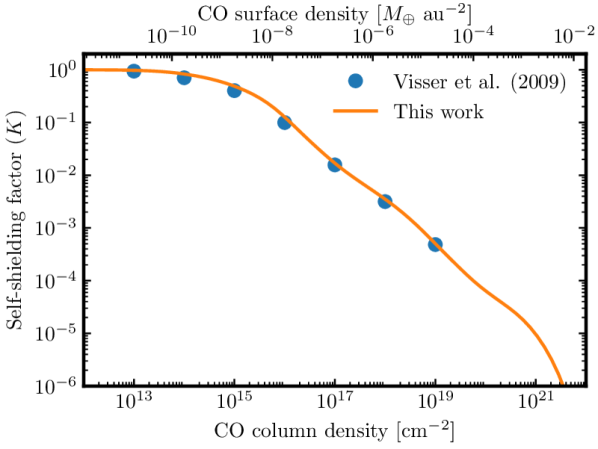
Figure 1: Self-shielding factor $K$ as a function of CO column density (orange). The blue points correspond to values in Table 6 of Visser et al. (2009) for an excitation temperature of 50 K, Doppler broadening of 0.3 km s^-1 and ¹²CO/¹³CO abundance ratio of 69.

Finally, we can write the photodissociation rate per molecule and the CO mass photodissociation rate per unit volume as

$$R_{\rm ph}(z)=\frac{R_{\rm ph,0}}{2}\int_{0}^{\pi}\sin(\theta)K\left(\frac{N^{\pm}_{\rm CO}}{|\cos(\theta)|}\right)e^{-N^{\pm}_{\rm CI}\sigma_{\rm CI}/|\cos(\theta)|}\mathop{}\!\mathrm{d}\theta$$ (17)

$$\dot{\rho}_{\rm ph}(z)=\rho_{\rm CO}(z)R_{\rm ph}(z).$$ (18)

Figure 2 shows the CO lifetime as a function of the CO vertical column density in the absence of CI. The solid lines correspond to the average lifetime defined as $\tau_{\rm CO,mean}=\int\rho_{\rm CO}(z)\mathop{}\!\mathrm{d}z/\int\dot{\rho}_{\rm ph}(z)\mathop{}\!\mathrm{d}z$, when considering the ISRF photons to enter the disc only vertically (thin line) or to be distributed in all directions (thick line). We find that the CO lifetime can be underestimated by a factor ${\sim}1.8$ for column densities above $10^{16}$ cm^-2 when the ISRF is assumed to enter the disc only vertically (where the optical depth is lowest) as done in Kral et al. (2019); Marino et al. (2020); Cataldi et al. (2020). The dashed lines show the CO lifetime at the midplane. These show that the midplane lifetime is longer by a factor $1.5-3$ for column densities above $10^{16}$ cm^-2. Thus considering the midplane lifetime as representative (as done in Kral et al., 2019; Marino et al., 2020) would overestimate the true CO lifetime in the disc. Nevertheless, both effects balance out and the average lifetime considering all directions of radiation is very close to the midplane lifetime when assuming all UV radiation enters the disc vertically.

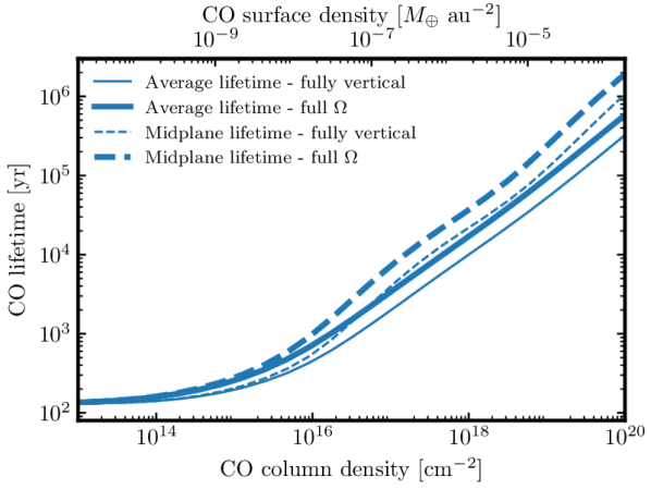
Figure 2: CO lifetime as a function of the CO vertical column density in the absence of CI. The solid lines show the average lifetime, while the dashed lines show the lifetime in the midplane. The thin and thick lines correspond to considering ISRF photons enter the disc only vertically or from all directions, respectively.

Figure 3 shows the CO average lifetime as a function of the CI column density in the absence of CO shielding. The solid lines correspond to a case where the CI gas is on a thin layer above and below all the CO gas (as assumed in Kral et al., 2019; Marino et al., 2020), whereas the dashed lines show a case where CI and CO are well mixed (as assumed in Cataldi et al., 2020). We find that the assumption on how CI is distributed has profound implications for the lifetime of CO gas, as pointed out by Cataldi et al. (2020). If CO and CI are well mixed, the average lifetime of CO increases only linearly with the CI column density as the photodissociation layer moves higher up in the disc. In fact, we find that self-shielding is more effective than CI-shielding for the same column density by a factor ${\sim}1.5$. This strong dependency of the CO lifetime on the CI vertical distribution means that it is crucial to study the vertical structure of the gas both theoretically and observationally to advance in our understanding of the gas evolution.

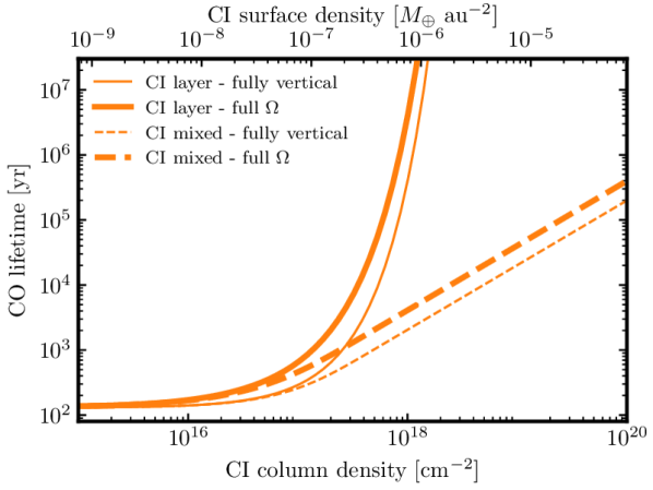
Figure 3: CO lifetime as a function of the CI vertical column density in the absence of CO shielding. The solid lines show the average lifetime when CI is in two surface layers above and below the CO gas. The dashed lines show a case where CO and CI are well mixed. The thin and thick lines correspond to considering ISRF photons enter the disc only vertically or from all directions, respectively.

The model presented above does not include the photodissociating UV photons from the star. These can dominate the UV radiation field at 100 au for early A-type stars. Nevertheless, Marino et al. (2020) showed that for the typical CO-rich debris discs where gas is detected, this component is negligible at tens of au due to the high column densities in the radial direction. Therefore, we omit it from our calculations.

2.3 C ionisation and recombination

The ionisation rate per CI atom is calculated as

$$R_{\rm ion}(z)=\frac{R_{\rm ion,0}}{2}\int_{0}^{\pi}\sin(\theta)e^{-N^{\pm}_{\rm CI}\sigma_{\rm CI}/|\cos(\theta)|}\mathop{}\!\mathrm{d}\theta,$$ (19)

where $R_{\rm ion,0}$ is ionisation rate per CI atom in the optically thin regime

$$R_{\rm ion,0}=\int\phi_{\lambda}\sigma_{\rm CI}\ \mathop{}\!\mathrm{d}\lambda,\\$$ (20)

and corresponds to an ionisation timescale of 100 yr. Recombination is calculated as

$$R_{\rm rc}(z)=\alpha_{\rm rc}(T)n_{\rm e^{-}}(z),$$ (21)

where $\alpha_{\rm rc}(T)$ is the recombination rate of CII that is dependent on the temperature and is taken from Badnell (2006). The number density of electrons $n_{\rm e^{-}}(z)$ is set equal to the number density of CII. In other words, we assume that electrons only originate from CI ionisation and that CII and electrons are co-located. Finally, the net ionisation rate is given by

$$\dot{\rho}_{\rm ion}(z)=\rho_{\rm CI}(z)R_{\rm ion}(z)-\rho_{\rm CII}(z)R_{\rm rc}(z).$$ (22)

2.4 Viscous evolution

As the gas viscously evolves, angular momentum is transported outwards while gas mass is mostly moved inwards. This process effectively removes gas from the centre of the belt forming an accretion disc interior to the belt and a decretion disc exterior to it. This process has been studied in detail using 1D simulations that model the radial evolution of gas (e.g. Kral et al., 2016; Moór et al., 2019; Marino et al., 2020). Here, we use a similar approach to Kral et al. (2019) and Cataldi et al. (2020), and we approximate the viscous removal of gas at the belt central radius with

$$\dot{\rho}_{\rm vis,i}(z)=\frac{\rho_{i}(z)}{t_{\rm vis}},$$ (23)

where $t_{\rm vis}$ is a viscous timescale. An expression for $t_{\rm vis}$ can be found by considering that in steady-state, the gas accretion rate ($3\pi\nu\Sigma$, Armitage, 2011) must be equal to the gas input rate $\dot{M}_{+}$, and that $\dot{\Sigma}_{+}$ must be equal to $\Sigma/t_{\rm vis}$. Combining these two equalities, we find

$$t_{\rm vis}=\frac{\sqrt{\pi}r\Delta r}{3\sqrt{2\ln(2)}\nu}\approx\frac{r\Delta r}{2\nu}.$$ (24)

With this definition, the steady-state surface density ($\dot{M}_{+}/(3\pi\nu)$) is independent of $\Delta r$, and matches the surface density obtained solving the radial viscous evolution and the analytic solution presented in Equation B13 in Metzger+2012 (valid when $\Delta r\xrightarrow{}0$). Note that when approximating the viscous evolution through Equation 23 (only truly valid at steady-state), the densities tend to grow faster and steady state is reached earlier than if we were to solve the viscous evolution radially. Finally, the kinematic viscosity is parametrized with the standard $\alpha$ viscosity as $\nu=\alpha c_{\rm s}H$ (Shakura & Sunyaev, 1973).

2.5 Gas vertical diffusion

The last effect to consider is the vertical diffusion, which will mix the different species. The diffusion term in Equations 1, 2, and 3 can be written as (Ilgner & Nelson, 2006; Armitage, 2011)

$$\dot{\rho}_{i,D}=\frac{\partial}{\partial z}\left[\rho D\frac{\partial}{\partial z}\left(\frac{\rho_{i}}{\rho}\right)\right],$$ (25)

where $D$ is the mass diffusivity, which we assume arises from turbulent mixing. Hence, we set $D$ equal to the vertical kinematic viscosity, $\nu_{\rm v}$, which is parametrised as $\alpha_{\rm v}c_{\rm s}H$. We will assume $\alpha_{\rm v}=\alpha$ unless otherwise stated, i.e. the vertical diffusivity is as strong as the radial kinematic viscosity. This means that the viscosity is isotropic, but it is possible that the vertical and radial viscosity and diffusion could differ (see discussion in §4.2). Therefore, we also explore scenarios where $\alpha_{\rm v}$ is independent of $\alpha$. Finally, we can define the vertical diffusion timescale as $t_{\rm diff}=H^{2}/D=1/(\alpha_{\rm v}\Omega_{\rm K})$, which translates to

$$t_{\rm diff}=1.3\times 10^{4}\ \mathrm{yr}\ \left(\frac{\alpha_{\rm v}}{10^{-2}}\right)^{-1}\left(\frac{r}{100\ \mathrm{au}}\right)^{3/2}\left(\frac{M_{\star}}{1.5\ M_{\odot}}\right)^{-1/2}.$$ (27)

3 Results

With the model presented above, we now proceed to simulate its evolution. We consider a system around a 1.5 $M_{\odot}$ star with a luminosity of 10 $L_{\odot}$. The system has a planetesimal belt centred at 100 au, with a FWHM of 50 au. We assume an alpha viscosity of $10^{-2}$, which translates to a viscous timescale of 1.5 Myr as defined in Equation 24. Note that although the viscosity parameter is kept constant, below we present the evolution for different values of $\alpha_{\rm v}$ and different gas input rates to cover the different scenarios. Our vertical grid consists of only one hemisphere since the disc is symmetric with respect to the midplane, and is divided into 50 bins from the midplane to 5 scale heights. The polar angle $\theta$ is sampled with 20 bins from 0 to $\pi$. We evolve the system for 10 Myr.

3.1 Without diffusion

Figure 4 shows a case in which CO gas is input at a rate of $10^{-3}$ $M_{\oplus}$ Myr^-1 and diffusion is switched off. The top panels show the vertical distribution of CO, CI, and CII at five different epochs. The three species have a vertical distribution that approximates a Gaussian. The bottom left panel shows the column density as a function of height. The horizontal dotted lines show the critical column density to shield the CO (below $z$) via self-shielding (blue) and CI-shielding (orange) by a factor $\geq e$. From this we can see that CO is only marginally shielded by CI as the column density of CI at the midplane is close to the critical column density. The bottom right panel shows the evolution of the surface density of the three species. This shows how the surface density of CO stays roughly constant at a value where the photodissociation rate is balanced by the CO input rate. While CO photodissociates, carbon is produced and quickly ionised in a 100 yr timescale. Ionised carbon dominates the first Myr of evolution, while CI dominates afterwards as recombination becomes more effective within 1.5 scale heights. After 3 Myr, the CI gas is close to steady state at surface density of $2\times{10^{-8}}\ M_{\oplus}$ au^-2. At this level CO is marginally shielded and its surface density increases by 50%. This case represents the systems with low CO masses where CO is released by planetesimals and destroyed in timescales of ${\sim}100$ yr like in $\beta$ Pic, HD 181327, and Fomalhaut (Dent et al., 2014; Marino et al., 2016; Matrà et al., 2017).

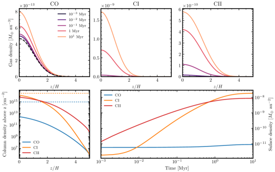
Figure 4: Evolution of CO, CI and CII for $\dot{M}_{+}=10^{-3}$ $M_{\oplus}$ Myr^-1, $\alpha=10^{-2}$ and no vertical diffusion. The top panels show the vertical density profile at different epochs as a function of $z/H$. The black dashed line in the top left panel shows the expected CO density if there was no shielding. The bottom left panel shows the vertical column density above $z$ as a function of $z/H$ (the total column density is twice the value reached at $z=0$) for CO (blue), CI (orange) and CII (red). The horizontal dotted lines show the critical column density of CO (blue) and CI (orange) to shield the CO underneath it by a factor $\geq e$. The bottom right panel shows the evolution of the surface density of CO, CI and CII.

Figure 5 shows a case with a hundred times higher CO release rate ($\dot{M}_{+}=0.1$ $M_{\oplus}$ Myr^-1). In this case CO becomes shielded after 1 Myr by CI and it reaches a photodissociation timescale of 6 Myr by the end of the simulation. This timescale is longer than the viscous timescale and thus CO is mainly lost via viscous evolution. As CI becomes optically thick to UV radiation, it forms a layer at $1.5H$ where CI production peaks, i.e. $\dot{\rho}_{\rm ph}(z)-\dot{\rho}_{\rm ion}(z)$ reaches its maximum. CII is mostly produced above this layer at $2H$ where carbon is still produced via photodissociation of new CO, and ionisation and recombination rates are comparable. This evolution confirms that it is possible that CI is in a layer above the midplane that is dominated by CO, as assumed in Kral et al. (2019) and Marino et al. (2020). This shielded case would correspond to the gas-rich discs, where CO masses and surface densities are found to be comparable to protoplanetary disc levels. Note that the height at which these layers are (relative to the scale height) will depend on the rate at which CO gas is released. The higher the release rate is, the higher these layers will be (see §3.3).

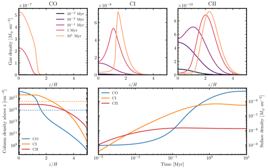
Figure 5: Same as Figure 4, but for $\dot{M}_{+}=0.1$ $M_{\oplus}$ Myr^-1, $\alpha=10^{-2}$ and no vertical diffusion.

3.2 With diffusion

Now we focus on the effect of vertical diffusion. Vertical diffusion happens on a timescale of $10^{4}$ yr for $\alpha=10^{-2}$ (Equation 27). It is worth noting that since $H$ is typically an order of magnitude smaller than $r$, vertical diffusion can be two orders of magnitude faster than viscous evolution. Vertical diffusion is, nevertheless, longer than CO photodissociation and ionisation timescales in the unshielded case. We thus do not see differences between a case with diffusion and without when the CO release rate is low, as in the case shown in Figure 4. On the other hand, if the gas release rate is high both ionisation and photodissociation rates become longer than the diffusion timescale, and thus CO and CI can easily mix.

Figure 6 shows this latter scenario where CO gas is released at a high rate of $0.1$ $M_{\oplus}$ Myr^-1. Diffusion mixes CO and CI, moving CO to upper layers where it becomes exposed and CI is transported towards the midplane reducing its effectiveness at shielding CO. Both CO and CI show a vertical distribution close to Gaussian with a standard deviation similar to $H$. Given the less effective shielding by CI, the photodissociation timescale drops to 0.09 Myr (almost a factor 100 shorter than the case without diffusion). The CO surface density, however, drops by a smaller factor close to 10. This difference is because in the scenario without diffusion, CO was being lost via viscous evolution (i.e. in a viscous timescale of ${\sim}1$ Myr), while with diffusion it is being lost via photodissociation. The CII distribution remains unaffected since carbon ionisation and recombination occur on a shorter timescales than diffusion.

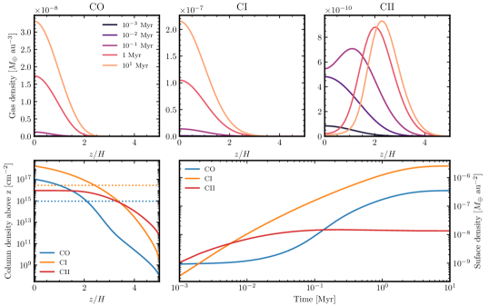
Figure 6: Same as Figure 4, but for $\dot{M}_{+}=0.1$ $M_{\oplus}$ Myr^-1, $\alpha=10^{-2}$ and with vertical diffusion.

It is also possible to consider a case where the vertical and radial values of $\alpha$ differ as mentioned in §2.5. In Figure 7 we show a case where vertical diffusion (parametrized now by $\alpha_{\rm v}$) is weaker and equal to $10^{-4}$. Since $H$ is a factor ${\sim}10$ smaller than the radius and width, the now hundred times weaker vertical diffusion leads to a vertical diffusion timescale similar to the viscous timescales and close to 1 Myr. At this critical value, mixing is significant causing the CI density to peak at the midplane but slow enough for CI to have a wide vertical distribution. Compared to the case with $\alpha_{\rm v}=\alpha=10^{-2}$, CO is better shielded and reaches a surface density similar to the case with no vertical diffusion. Therefore, we conclude that for $\alpha_{\rm v}<\alpha(H/r)^{2}$ vertical diffusion plays a minor role. Conversely, if $\alpha_{\rm v}>\alpha(H/r)^{2}$ and the diffusion timescale is shorter than the age of the system, vertical diffusion mixes CO and CI. For systems younger than the diffusion timescale ($\sim 10^{2}/\alpha_{v}$ yr at 100 au, Equation 27), or systems in which gas has been released for a shorter timescale, vertical mixing will not be able to effectively mix CO and CI.

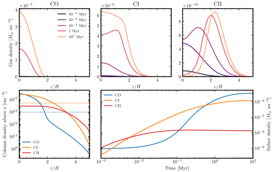
Figure 7: Same as Figure 4, but for $\dot{M}_{+}=0.1$ $M_{\oplus}$ Myr^-1, $\alpha=10^{-2}$ and with a vertical diffusion strength of $\alpha_{\rm v}=10^{-4}$.

3.3 The vertical distribution of CO and CI

In order to understand how the vertical distribution of CO and CI depend on the gas input rate and $\alpha_{\rm v}$ we run exogas for a sample of different values fixing $\alpha=10^{-2}$ and evolving the system until it reaches steady state. The main effect of changing the gas input rate is to change the steady state surface density of gas ($\Sigma_{\rm SS}$), which is simply the product of the gas input rate ($\dot{\Sigma}_{+}$ as defined in Equation 8) and the viscous timescale. Therefore, below we will focus on how the CO and CI distribution change as a function of this steady state surface density. Figure 8 shows where the CO (blue) and CI (orange) densities peak (solid lines) as a function of the steady state surface density. The shaded area represents the region where the density is at least 60% of the peak density (equivalent to a $\pm H$ range for a Gaussian distribution), and the dashed lines the height at which CO and CI become optically thick to photodissociating radiation in the vertical direction (i.e. the $\tau=1$ layer for each species).

The top panel shows cases with low vertical diffusion ($\alpha_{\rm v}=\alpha/1000=10^{-5}$). For low gas densities, CO and CI have the same vertical distribution as shown in Figure 4. As the surface density increases, we find an intermediate stage where CI gas becomes optically thick and can shield CO, which becomes highly peaked at the disc midplane. At higher surface densities, the CI density peaks in a surface layer at a height just below its $\tau=1$ layer, which increases with the surface density. This layer traces the location where the CO photodissociation rate is the highest. As CO is well shielded under this layer, the CO vertical extent becomes wider, closer to a Gaussian and with a standard deviation equal to $H$.

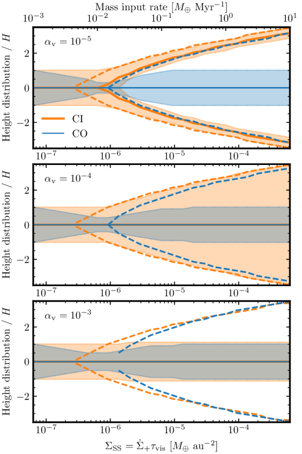
Figure 8: Vertical distribution in steady state of CO (blue) and CI (orange) normalized by the scale height ($H$) as a function of the steady state surface density of gas, in a case with $\alpha=10^{-2}$. The solid line shows where the density distribution peaks, while the shaded region represents the region where the density is at least 60% of the peak density ($1\sigma$ drop). The dashed lines represent the height at which CI and CO become optically thick to photodissociating radiation in the vertical direction. The top, middle, and bottom panels show scenarios where $\alpha_{\rm v}$ is $10^{-5}$, $10^{-4}$, and $10^{-3}$, respectively. The upper x-axis in the top panel shows the mass input rates as reference. Note that the orange solid line in the middle and bottom panels lies behind the solid blue line.

The middle panel shows cases with an intermediate vertical diffusion ($\alpha_{\rm v}=\alpha/100=10^{-4}$). The behaviour is similar to the one with low vertical diffusion, e.g. the CO vertical distribution and $\tau=1$ layer are almost identical. However, the CI distribution now peaks at the midplane, still extending to heights similar to the case with low vertical diffusion. This intermediate case demonstrates how even if the CI density peaks at the midplane, the CI equivalent scale height can be much larger than the true gas scale height.

The bottom panel shows a case with a high vertical diffusion ($\alpha_{\rm v}=\alpha/10=10^{-3}$). In this case, both CO and CI have an almost identical vertical distribution, except in the intermediate stage when CI starts to become optically thick. In this range of surface densities, CO is moderately shielded near the midplane and thus its density strongly peaks at $z=0$. Note that the diffusion timescale is not short enough compared to the photodissociation timescale to smear out this peak. Only for $\alpha_{\rm v}{\sim}1$, the vertical diffusion timescale would become ${\sim}100$ yr, i.e. comparable to the CO photodissociation timescale, and thus short enough to widen the vertical distribution of CO in this range of surface densities. Note that a stronger vertical diffusion (e.g. $\alpha_{\rm v}=\alpha=10^{-2}$) leads to very similar results where CO and CI are well mixed. The main difference is that at the intermediate stage the vertical spread of CO is slightly wider.

Finally, although the example shown in Figure 8 shows a case with $\alpha=10^{-2}$, we find similar results for higher and lower $\alpha$’s if we keep $\alpha_{\rm v}/\alpha$ constant. An example of this is shown in the Appendix B, where we show that with $\alpha=10^{-1}$ the same vertical structures are obtained. In other words, for a fixed $H/r$ whether CI will form a surface layer or will be bound to the midplane will ultimately depend on the ratio $\alpha_{\rm v}/\alpha$, the viscosity (or gas removal timescale) and the gas production rate. As mentioned in §3.2, in systems younger than the vertical diffusion timescale (Equation 27), i.e. not yet in steady state, the CI could form a surface layer regardless of the ratio $\alpha_{\rm v}/\alpha$ if the gas surface density is high enough for CI to become optically thick in the vertical direction.

3.4 The surface density of CO and CI

With a better understanding of how the vertical distribution of CI depends on $\alpha_{\rm v}$, we now focus on how the surface density of CO and CI will depend on $\alpha_{\rm v}$. Figure 9 shows the surface density of CO (blue) and CI (orange) as a function of the steady state surface density of gas, for different values of $\alpha_{\rm v}$, assuming $\alpha=10^{-2}$. As expected, the lower $\alpha_{\rm v}$ is, the better CI is at shielding CO as it is mostly in a surface layer that absorbs most UV photons. The upper and lower black diagonal lines show the expected surface density of CO if it is lost through viscous evolution or if it is unshielded and lost through photodissociation, respectively. For a low $\alpha_{\rm v}$ (solid line), as $\Sigma_{\rm SS}$ increases the CI production rate stalls as most UV photons are absorbed by CI rather than CO. This is why the surface density of CI is almost constant for $\Sigma_{\rm SS}\geq 10^{-6}\ M_{\oplus}$ au^-2. This also causes the CO lifetime to increase exponentially up to a viscous timescale, and the surface density quickly converges to the upper black line.

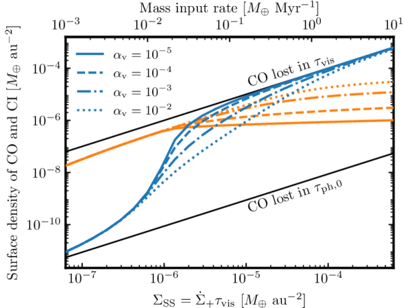
Figure 9: Surface density of CO (blue) and CI (orange) as a function of the steady state surface density of gas, in a case with $\alpha=10^{-2}$. The solid, dashed, dot-dashed and dotted lines represent cases with $\alpha_{\rm v}=10^{-5}$, $10^{-4}$, $10^{-3}$, and $10^{-2}$, respectively. The upper and lower black solid lines represent the maximum and minimum surface density of CO, i.e. when it is lost in a viscous timescale or unshielded and lost in a 130 yr photodissociation timescale. The upper x-axis shows the mass input rates as reference.

On the other hand, as described before, with a high value of $\alpha_{\rm v}$ (dotted line) CI is well mixed with CO and thus it is not as effective at shielding it from photodissociating radiation. Thus, for the same $\Sigma_{\rm SS}$ or gas input rate, the CO surface density is much lower than in the case with a weak vertical diffusion. This is effectively the result obtained by Cataldi et al. (2020).

The difference between the blue curves is the largest near $\Sigma_{\rm SS}=2\times 10^{-6}\ M_{\oplus}$ au^-2, where the surface density of CO for $\alpha_{\rm v}=10^{-5}$ is ${\sim}30$ times larger than for $\alpha_{\rm v}=10^{-2}$. How big this difference is also depends on $\alpha$. The lower the viscosity, the larger this difference becomes as shielding can extend the CO lifetime to an even longer viscous timescale.

4 Discussion

In this section we discuss the implications of our findings, what is known about vertical diffusion in circumstellar discs, and the level of ionisation of the gas obtained from our simulations. We also discuss the effect vertical diffusion can have on the vertical settling of dust and on the radial evolution of CO, how high resolution observations could constrain the strength of vertical diffusion, but might be unable to constrain the gas scale height, and finally, we discuss some of the limitations of our model.

4.1 Implications for shielded/hybrid discs

As pointed out by Cataldi et al. (2020) and demonstrated in detail here, if CO and CI are well mixed shielding is much less effective than if CI is in a surface layer. To achieve the same level of shielding, much higher quantities of CI gas are needed. However, CI observations of gas-rich discs seem to suggest lower CI quantities than those needed if CO and CI are well mixed. Two scenarios might solve this tension. On one hand, Cataldi et al. (2020) suggested that if CI was captured by dust grains and then used to re-form CO that is then released, this could maintain a high CO production rate in the system. In this recycling scenario, CO would be predominately self-shielded. This scenario, however, still needs to be tested via physical simulations or experiments. On the other hand, the gas could be primordial or hybrid in origin, containing still large amounts of hydrogen that shield the CO (Kóspál et al., 2013). Note that although the CI mass has been constrained, its value is still largely dependent on assumptions such as its temperature and vertical structure that can change its optical depth when viewed close to edge-on. Therefore, it is possible that the real mass of CI in the gas-rich discs is much larger than the current observational estimates.

If diffusion is weak, nevertheless, we expect the CI density to peak above and below the CO-dominated midplane, as implicitly assumed in the simple shielded secondary scenario presented by Kral et al. (2019). A weak diffusion could thus explain the population of gas-rich discs and account for the current CI mass estimates. Unfortunately, there are no clear predictions for how strong vertical diffusion will be (see §4.2 below). This will ultimately depend on the relative strength of the turbulence in the vertical and radial direction. Therefore, high-resolution ALMA observations are crucial since they reveal the true nature of gas-rich debris discs and provide constraints on the hydrodynamics (see §4.6).

4.2 Vertical diffusion

Since the strength of the vertical diffusion in debris discs is not well known, we may look for some guidance from the study of protoplanetary discs, keeping in mind that the gas densities and especially the dust optical depths are significantly higher than in debris discs. One way to constrain the vertical diffusion in protoplanetary discs is by considering the disc chemistry. For example, in order to explain the high CH₃CN abundance observed towards MWC 480, the disc model by Öberg et al. (2015) requires efficient vertical transport ($\alpha_{\rm v}{\sim}10^{-3}$–$10^{-2}$) of CH₃CN ice from the midplane to UV-exposed regions in the disc atmosphere where the ice can be photodesorbed. Similarly efficient vertical mixing is also believed to contribute to the observed C depletion in protoplanetary discs by transporting CO from the disc atmosphere to the midplane where it can freeze out and be sequestered into pebbles (e.g. Kama et al., 2016; Van Clepper et al., 2022). Dust settling has also been used to constrain vertical diffusion. For example, Pinte et al. (2016) report that their dust settling model best fits the small dust scale height of the HL Tau protoplanetary disc if weak vertical diffusion is assumed ($\alpha_{\rm v}$ a few times $10^{-4}$).

Recent observations aimed at detecting non-thermal gas motion form CO line emission suggest that relatively weak turbulence (corresponding to $\alpha\lesssim 10^{-3}$) may be common in protoplanetary discs (Flaherty et al., 2018; Flaherty et al., 2020). In general, it is often assumed that $\alpha_{\rm v}$ is approximately equal to the turbulent $\alpha$ parameter. This can be justified from numerical simulations of protoplanetary discs subject to the magneto-rotational instability (MRI), showing that $\alpha_{\rm v}$ is usually within an order of magnitude of $\alpha$ (e.g. Okuzumi & Hirose, 2011; Zhu et al., 2015; Xu et al., 2017). To the best of our knowledge, the only study looking at the MRI in debris discs was presented by Kral & Latter (2016). They showed that the MRI could be at work in the debris disc around $\beta$ Pictoris, although a weak magnetic field would be sufficient to stabilise the disc. However, their results might not be directly applicable to the CO-rich discs we consider here due to the significantly higher gas densities and lower ionisation compared to the disc around $\beta$ Pic (see §4.3).

As a further complication, the turbulence strength could vary vertically as the ionisation level increases with $z$ (Flock et al., 2015; Delage et al., 2021). Also, if turbulent motion is driven by a mechanism different from the MRI, $\alpha$ could be very different from $\alpha_{\rm v}$. Numerical simulations by Stoll et al. (2017) show that turbulence induced by the vertical shear instability could be highly anisotropic ($\alpha_{\rm v}$ more than two orders of magnitude larger than $\alpha$).

In summary, the strength of vertical diffusion in debris discs is essentially unknown. Thus, in this study we explored a range of plausible values for $\alpha_{\rm v}$ to understand the gas evolution in different regimes. Future observations of highly-inclined gas-rich debris discs could provide the first constraints on $\alpha_{\rm v}$ and the hydrodynamics (see §4.6).

4.3 Ionisation fraction

As discussed above, one possible driver of vertical (and radial) diffusion in debris discs is turbulence due to the MRI. Well-ionised debris discs such as $\beta$ Pic may be unstable to the MRI, provided that the magnetic field is not too strong (Kral & Latter, 2016). If, however, the ionisation fraction is too low, the gas decouples from the magnetic field and the disc is stable to the MRI (in protoplanetary discs, such regions are known as “dead zones”; Gammie, 1996).

Consideration of the disc vertical structure is important for the calculation of the ionisation fraction in debris discs. Kral et al. (2019) found that the ionisation fraction near the disc midplane can be several orders of magnitude lower than that at the disc surface, due to the self-shielding of the atomic carbon. This effect is also present in the models presented in this paper (see Figure 10), where both the atomic carbon and CO in the upper disc layers shield the disc midplane from the ISRF. We find that the ionisation fraction at the disc midplane can vary greatly with the disc mass (which is, at fixed $\alpha$, proportional to the gas mass input rate shown in Figure 10). In a more massive disc, the disc midplane is better shielded and this results in both lower rate of carbon production and lower ionisation rate of the produced carbon. Vertical diffusion also influences the midplane ionisation fraction, to a lesser degree. We find that the relationship between the degree of vertical diffusion (i.e., $\alpha_{\rm v}$) and the midplane ionisation fraction is non-monotonous. This is due to the relative importance of two competing effects. As the vertical diffusion coefficient first increases from $10^{-5}$ to $10^{-4}$ (solid to dashed line), diffusion is strong enough for CI from upper layers to diffuse downwards decreasing the shielding of CO, which in turn increases the CO photodissociation rate and thus the surface density of CI. The higher CI surface density translates to a higher optical depth that lowers the ionisation rate of carbon and thus the ionisation fraction. However, as $\alpha_{\rm v}$ increases further (dashed to dotted line), the diffusion timescale is short enough for ionised carbon to diffuse downwards, increasing the ionisation fraction at the midplane despite the much lower ionisation rate.

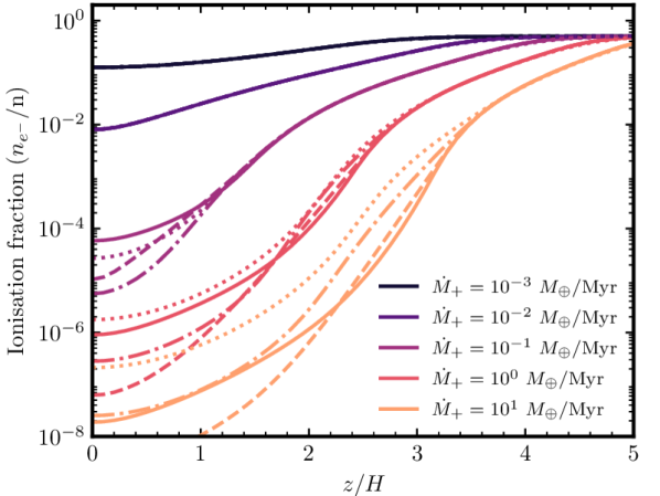
Figure 10: Ionisation fraction as a function of height for a disc with $\alpha=10^{-2}$. The different colours correspond to different gas input rates. The solid, dashed, dot-dashed, and dotted lines represent cases with $\alpha_{\rm v}=10^{-5}$, $10^{-4}$, $10^{-3}$, and $10^{-2}$, respectively. The ionisation fraction is calculated as the number density ratio between CII (equivalent to the electron number density) and CO+CI+CII+O.

This variation of the ionisation fraction with height above the disc midplane is reminiscent of the ionisation state of protoplanetary discs. In vast regions of protoplanetary discs cosmic rays and stellar X-rays ionise only the disc upper layers, but do not reach the disc midplane, leading to MRI-dead zones (Gammie, 1996; Igea & Glassgold, 1999). If the midplane regions of debris discs are similarly MRI-dead, any vertical mixing or radial diffusion driven by the MRI would be considerably weaker than in a well-ionised disc. However, the low midplane ionisation fractions (as low as ${\sim}10^{-8}$) we find here may still be well above the critical value required to make the disc unstable to the MRI. In protoplanetary discs, that critical value can be of the order of only $10^{-12}$ (e.g. Gammie, 1996). The stability of weakly ionised debris discs against the MRI remains to be explored, taking into account the chemical composition that differs largely from protoplanetary discs and to a lesser degree from well ionised debris discs considered by Kral & Latter (2016).

4.4 Dust scale height

Whilst in this paper we have focused only on the gas evolution, the dynamics and evolution of dust can be strongly affected by the presence of gas (Takeuchi & Artymowicz, 2001; Thébault & Augereau, 2005; Krivov et al., 2009; Lyra & Kuchner, 2013; Pearce et al., 2020). In particular, Olofsson et al. (2022) recently showed how gas can cause dust grains to settle towards the midplane if their inclinations are damped by the gas in a timescale (the stopping time) shorter than their collisional lifetime. This effect is strongest for the smallest grains in contrast to what happens in protoplanetary discs where it is the largest grains that readily settle towards the midplane. In debris discs the gas densities are low enough such that all grains larger than the blow-out size have Stokes numbers larger than unity (see Figure 11 in Marino et al., 2020), therefore all bound grains are decoupled from the gas. However, only the smallest grains have stopping times shorter than their collisional lifetime. Therefore, if gas densities are high enough we expect small grains to be more concentrated towards the midplane than large grains and planetesimals.

One important effect that was neglected by Olofsson et al. (2022) is the stirring by turbulent diffusion that could reduce the amount of inclination damping (Youdin & Lithwick, 2007). In the presence of turbulent diffusion (as considered in this paper), the scale height of dust is expected to be (Equation 24 in Youdin & Lithwick, 2007)

$$H_{\rm d}=H\sqrt{\frac{\alpha_{\rm v}}{\rm St}}\sqrt{\frac{\rm 1+St}{\rm 1+2St}},$$ (28)

where St is the Stokes number or the dimensionless stopping time. The Stokes number is defined as $\frac{\pi}{2}\frac{a\rho_{\rm s}}{\Sigma}$, where $a$, $\rho_{\rm s}$ and $\Sigma$ are the grain size, the internal density of grains and the gas surface density, respectively. Since we expect $\mathrm{St}\gg 1$, we have $H_{\rm d}\approx H\sqrt{\frac{\alpha_{\rm v}}{\rm 2St}}$. We can evaluate this for a gas rich debris disc with a surface density of $10^{-5}\ M_{\oplus}$ au^-2 (i.e. $M_{\rm gas}{\sim}1\ M_{\oplus}$) to obtain

$$\frac{H_{\rm d}}{H}=0.1\left(\frac{a}{\rm 1\ \mu m}\right)^{-1/2}\left(\frac{\alpha_{\rm v}}{10^{-2}}\right)^{1/2}\left(\frac{\Sigma}{10^{-5}\ M_{\oplus}\ \mathrm{au}^{-2}}\right)^{1/2}\left(\frac{\rho_{\rm s}}{\rm 1\ g\ cm^{-3}}\right)^{-1/2}.$$ (29)

This means that although gas drag will damp the inclinations of $\mu$m-sized grains, these will not completely settle towards the midplane if the gas surface densities are high ($\gtrsim 10^{-5}$ $M_{\oplus}$ au^-2) and turbulent diffusion is strong ($\alpha_{\rm v}\gtrsim 10^{-2}$). Note that these equations are only valid for those dust grains with a collisional lifetime much longer than the stopping time. Therefore, observational estimates of the scale height of gas and small dust grains could help to constrain the strength of vertical diffusion and gas models.

4.5 Radial evolution

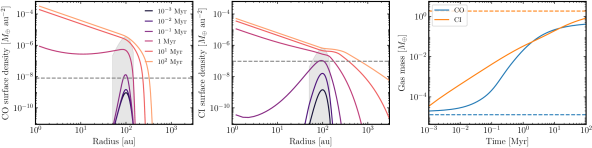
Figure 11: Radial evolution of the surface density of CO (left), CI (middle), and their masses (right), in a system where CO gas is released at a rate of 0.1 $M_{\oplus}$ Myr^-1 from a belt centred at 100 au and 50 au wide (FWHM) (grey shaded region), with $\alpha=10^{-2}$. The top panel represents a case where CI is in the surface of the disc, while in the bottom panel CO and CI are perfectly mixed. The horizontal grey dashed lines represent the surface density at which CO becomes shielded by a factor $e$. The horizontal blue and orange lines in the right panels show the expected steady-state mass if CO was unshielded.

Throughout this paper we have shown the importance of the vertical evolution on the effectiveness of shielding of CO by atomic carbon. Whether carbon is well mixed or in a layer has profound implications for how the gas will evolve. Here, we investigate how the radial evolution could be affected by the vertical diffusion of gas. To this end, we focus on two extreme scenarios: one where CI is in a layer completely far above and below the CO-rich midplane, and another where CO and CI are well mixed. For both scenarios we consider a system where CO gas is released at a rate of 0.1 $M_{\oplus}$ Myr^-1 in a belt centred at 100 au and 50 au wide (FWHM), around a 1.5 $M_{\odot}$ star (10 $L_{\odot}$), and with $\alpha=10^{-2}$.

We solve the radial evolution of CO and CI in these two scenarios using the radial module of the python package exogas that is based on the model developed in Marino et al. (2020). Because the photodissociation of CO strongly depends on the disc vertical structure, which this module does not solve, we need to precompute the CO photodissociation timescales. We do this using the vertical evolution module for a grid of 50x50 different surface densities of CO and CI that are logarithmically spaced. Here is where the two scenarios differ. In order to compute these timescales, we need to define the vertical distribution of CO and CI. First, we assume all CI is distributed in two surface layers on top of and below the CO gas. Second, we assume CI and CO are well mixed. In Figure 3 we showed how the CO lifetime could be very different in these two scenarios. exogas then uses these precomputed grids and interpolates its values to estimate the CO photodissociation timescale. These grids provide realistic photodissociation timescales similar to the ones obtained through photon counting (Cataldi et al., 2020), but that also account for UV radiation entering the disc at different angles which lengthens the CO lifetime by a factor ${\sim}2$ (see §2.2).

Figure 11 shows the surface density profiles of CO (left), CI (middle), and the mass evolution of CO and CI as a function of time. The top panels show the case where CI is in a surface layer, and thus the shielding is most effective. Once CI reaches a high enough surface density ($10^{-7}$ $M_{\oplus}$ au^-2), CO starts to become shielded. With a longer lifetime, CO viscously evolves spreading inwards and outwards beyond the planetesimal belt where CO is released (grey shaded region). The resulting surface densities at the belt center after 10 Myr of evolution are very similar to those obtained when simulating the vertical evolution without vertical diffusion (§3.1). Similar to the simulation results in Marino et al. (2020), we find a plateau in the CI surface density from 100 to 200 au after 100 Myr of evolution. This feature can be understood by examining the top left and middle panels. In the first 1 Myr of evolution, CI accumulates forming an accretion disc that is massive enough to shield CO within 150 au, allowing it to accumulate, viscously accrete, and dominate the gas surface densities. Beyond the belt centre, the released CO gas slowly flows outwards, but at a timescale much longer than the CO lifetime (which decreases exponentially with radius), resulting in an exponential drop in the surface density of CO. In this drop between $100-300$ au the gas composition changes from being CO dominated to being carbon and oxygen dominated. It is the balance between the decrease in the overall gas surface density and the increase in the abundance of CI that creates the plateau. Therefore the plateau starts at the belt centre (where gas starts to flows outwards) and stops where CI and OI dominate the bulk of the gas density.

If CI and CO are well mixed (bottom panel) the average CO lifetime at the belt centre is only 0.02 Myr, which is too short compared to the viscous timescale (6 Myr). This is why CO does not viscously spread significantly after 100 Myr. This scenario is the most problematic for explaining gas-rich discs since their estimated CI levels would not be enough to shield CO (Cataldi et al., 2020). We note one caveat in this calculation that results in an underestimation in the level of shielding compared to the case with a strong diffusion ($\alpha_{\rm v}=\alpha$) and a high gas input rate (0.1 $M_{\oplus}$ Myr^-1) presented in §3. We assume that CI and CO are perfectly mixed, however, when simulating the vertical evolution with $\alpha_{\rm v}=\alpha$, CO is still more concentrated towards the midplane than CI. This is because the photodissociation timescale in the top layers is still shorter than the diffusion timescale, therefore CO becomes depleted there relative to the midplane. This behaviour is also shown in Figure 8 for values of $\Sigma_{\rm ss}=10^{-6}$ $M_{\oplus}$ au^-2. The carbon-dominated upper layer can significantly contribute to shielding CO. In order to completely mix CO and CI, the diffusion timescale should be shorter than the unshielded photodissociation timescale. At ${\sim}100$ au, that would only be obtained with $\alpha\gtrsim 10^{-1}$. Therefore, perfect mixing might never happen in debris discs unless they are strongly turbulent in the vertical direction.

We conclude that the vertical structure of the gas has a large impact on the radial evolution. The two extreme scenarios explored here lead to significantly different results, particularly for the CO distribution. Constraining the vertical structure of the gas is thus crucial to advance our understanding of the gas evolution in debris discs.

4.6 Observability

In this section we produce radiative transfer predictions and discuss how the vertical distribution of CO and CI would translate into real observations. To this end, we use RADMC-3D that allows to produce synthetic images of dust and gas emission based on several parameters and input files such as the dust distribution, opacity, gas distribution, velocity field, molecular information, stellar spectrum, etc. We produce these files and run RADMC-3D calculations using the python package disc2radmc (based on Marino et al., 2018), which allows to define these input files and run multiple RADMC-3D calculations in a simple and concise manner.

We focus on and compare the two main scenarios presented in §3. In these two scenarios, CO gas has been released at a rate of 0.1 $M_{\oplus}$ Myr^-1 for 10 Myr and $\alpha=10^{-2}$ (i.e. it is in steady state). They differ in that in one gas evolves without vertical diffusion, while in the other there is strong vertical diffusion ($\alpha_{\rm v}=\alpha=10^{-2}$). Since our vertical simulations presented above were one dimensional, we need to extrapolate their density distribution of CO and CI in order to define their density as a function of $r$ and $z$. For simplicity, we assume the vertical distribution (relative to $H(r)$) is independent of radius and the surface density distribution of both species follows a Gaussian distribution centred at 110 au and with a standard deviation of 34 au (FWHM of 80 au). We further assume a scale height of 5 au at 100 au, which scales linearly with radius, and a turbulence corresponding to $\alpha=10^{-2}$ that broadens slightly the line emission. Note that although the true gas temperature could be different (hotter or colder) and the mean molecular weight higher (if CO dominated), the vertical distribution relative to $H$ will remain roughly the same as shown in §4.8. This means that while the vertical extent of CO and CI is uncertain and could vary as $\sqrt{T/\mu}$, their predicted morphologies presented below are robust. A higher (lower) temperature would only stretch (compress) their vertical distributions. Finally, we assume a 1.7 $M_{\odot}$ central star, at a distance of 133 pc, and that is viewed edge-on. The radial distribution, stellar mass, and distance approximate the values for HD 32297, a gas-rich edge-on disc (Greaves et al., 2016; MacGregor et al., 2018; Cataldi et al., 2020).

Under these assumptions and density distributions, we compute synthetic images of CO J$=2-1$ ($\lambda=1300$ $\mu$m) and CI ${}^{3}\mathrm{P}_{1}-^{3}\mathrm{P}_{0}$ emission ($\lambda=609$ $\mu$m), both readily accessible through ALMA observations. When calculating the emission from these species, RADMC-3D assumes Local Thermodynamic Equilibrium (LTE), i.e. the population levels of each gas species are set by the local temperature. It is well-known that non-LTE can be important when gas densities are low (Matrà et al., 2015), but the densities considered here should be high enough for the different energy levels to be collisionally excited and in thermal equilibrium.

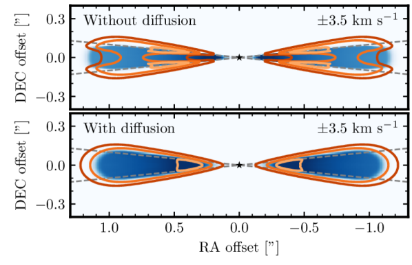
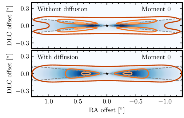
Figure 12: Radiative transfer prediction of CO and CI emission for an edge-on disc. The top two panels show the emission at line-of-sight velocities of $\pm 3.5$ km s^-1, while the bottom two show the moment 0 (velocity integrated emission). CO J$=2-1$ emission is shown in blue colours, while CI ${}^{3}\mathrm{P}_{1}-^{3}\mathrm{P}_{0}$ emission is shown in orange contours at 10, 50 and 90% of the peak value. The first/third and second/fourth panels show a case without and with vertical diffusion (respectively), assuming $\alpha=10^{-2}$ and $\dot{M}^{+}=10^{-1}$ $M_{\oplus}$ Myr^-1 after 10 Myr (in steady state). The grey dashed line represent 2 scale heights from the midplane.

Figure 12 shows the expected emission at line-of-sight velocities of $\pm 3.5$ km s^-1 (close to the Keplerian velocity at the belt centre of 3.7 km s^-1) and the moment 0 (i.e. the velocity integrated emission) for a case without and with diffusion (scenarios presented in Figures 5 and 6, respectively). The CO intensity is displayed with a blue colour map, while CI is shown with orange contours. In both the channel maps and moment 0’s we find a similar morphology. Without diffusion, the CO emission peaks at the midplane and is located within 2 scale heights from the midplane (grey dashed lines), while CI emission is almost absent within one scale height and peaks near the upper and lower edges of the CO emission. Note that the height at which this happens, relative to the scale height, can vary depending on the gas input rate and viscosity (§3.3). Since CO is very optically thick, its emission peaks towards the inner regions where the gas is hotter. Conversely, with diffusion the CI and CO emissions peak in the midplane displaying a very similar intensity distribution. The only difference is that CI emission extends vertically slightly further compared to CO since the latter has a slightly narrower vertical distribution due to photodissociation. Finally, the observed vertical morphology is not sensitive to the radial distribution of CO and CI. A different radial distribution would change how the emission is distributed radially, but the vertical morphology would still be the same. This is especially true for individual channel maps where each pixel traces approximately a single radius.

These radiative transfer simulations show that it is possible to distinguish these two scenarios by looking at the vertical distribution of CO and CI. Both emission lines have been already detected and resolved radially in multiple shielded discs. So far, only Hughes et al. (2017) and Higuchi et al. (2019) have tried to constrain the vertical extent of CO and CI. Doing a similar analysis for both lines, Higuchi et al. (2019) found their heights to be consistent with each other, although with large uncertainties that prevent assessing the strength of vertical diffusion. Future observations at high-resolution should reveal if CI is located in a surface layer and thus indicate the strength of vertical diffusion. Note that with images that do not resolve the vertical distribution of CO and CI, it is impossible to distinguish between these two scenarios due to the unknown gas temperatures and gas scale height.

Whilst in the radiative transfer predictions presented above we focus in an edge-on case, vertical information can also be obtained for discs with moderate inclinations. It has been shown that the characteristic height of emission lines can be obtained from line-of-sight velocity maps, as well as from individual channels (e.g. Teague et al., 2018; Pinte et al., 2018; Casassus & Pérez, 2019; Izquierdo et al., 2021). Therefore, ALMA observations at a resolution comparable or better than the disc scale height offer a unique chance to determine how strong vertical diffusion is, and thus how important shielding by CI is.

4.7 Is the observed gas scale height a good indicator of gas origin?

It has been suggested that a powerful way to determine the origin of gas in debris discs is to measure its scale height (e.g. Hughes et al., 2017; Kral et al., 2019; Smirnov-Pinchukov et al., 2021). By knowing the scale height and the temperature of a disc, one could estimate the mean molecular weight. This would allow to determine if the gas is dominated by molecular Hydrogen or by heavier species such as C, O, or CO (e.g. Hughes et al., 2017). In addition to the difficulty of estimating the gas kinetic temperature, a key problem lies in measuring the gas scale height. To measure it, one would need to use a gas tracer such as CO or CI, but as shown here the vertical distribution of these species can differ significantly from the gas true vertical distribution. For example, in the results presented in §3.3 we found that the distribution of CO can be skewed towards the midplane due to its higher shielding at the midplane if vertical mixing is weak, mimicking a small scale height. A similar phenomenon could occur in a primordial gas scenario as well if vertical diffusion is weak since the CO lifetime will also be longer near the midplane. This means that the small CO scale height measured in 49 Ceti by Hughes et al. (2017) might be very different from the true gas scale height (even if primordial). Hence one should be careful interpreting a small CO scale height as evidence of a high mean molecular weight (and thus gas of secondary origin). On the other hand, the vertical distribution of CI can be much wider mimicking a larger scale height. Moreover, a high optical depth would rise the emitting surface of optically thick species making the apparent vertical distribution wider than in reality. Therefore, we recommend that scale height values derived directly from observations should be used with caution, and ideally interpreted using gas models and radiative transfer simulations. Otherwise, estimates could suffer from great systematic errors.

4.8 How does temperature affects the evolution?

Throughout the paper we have assumed a gas temperature equal to the blackbody equilibrium temperature at 100 au of 50 K, which translates to a scale height of 5 au. However, the gas temperature could be significantly different from the blackbody and dust temperature in reality, depending on the gas heating and cooling rates (e.g. Kral et al., 2016). Therefore, in this section we examine the evolution of the gas with a temperature 10 times higher (500 K) in order to understand its effects. The increased temperature changes the sound speed, which in turn changes other important quantities. First, the gas scale height is increased by a factor $\sqrt{10}$ from approximately 5 au to 15 au. Second, the viscosity is 10 times higher (as we keep $\alpha$ fixed), which translates to a viscous timescale 10 times shorter.

We now compare the gas evolution in the case of no vertical diffusion and a high gas input rate, as presented in §3.1 and in Figure 5. In order to focus on the effect of the temperature alone, we increase the mass input rate by a factor 10 to keep the total gas surface density in steady state constant. Figure 13 shows the evolution of CO, CI and CII for $T=500$ K. The dashed lines show our standard model with $T=50$ K for comparison. The grey dashed lines in the top panels have been scaled by a factor $1/\sqrt{10}$ to account for the difference in scale height and ease the comparison. We find that the gas evolution is very similar to the case with a lower temperature. The main differences are that the CI surface density is ${\sim}30$% smaller, the CII surface density is a factor 5 greater, the CO, CI and CII volumetric densities are lower (due to the increased scale height), and that the steady state is reached earlier due to the 10 times shorter viscous timescale. The increase in the surface density of CII (and decrease of CI) can be explained by the lower volumetric densities and higher temperature that decrease the recombination rate of CII. Conversely, reducing the temperature (or increasing $\mu$) would have the opposite effect: CII recombination rates would be higher, increasing (reducing) the surface density of CI (CII). These findings confirm that the evolution of CO and CI is more sensitive to the column (or surface) densities rather than the volumetric densities.

If we considered vertical diffusion, the increase in the temperature would leave the vertical diffusion timescale unchanged ($1/(\alpha_{\rm v}\Omega_{\rm K})$). However, the vertical diffusion timescale relative to the viscous timescale would become longer, and thus the CO and CI would become less mixed. We note that this conclusion is only valid if $\alpha$ and $\alpha_{\rm v}$ are kept fixed. The high uncertainty in the relative values of $\alpha_{\rm v}$ and $\alpha$, and their dependence on the temperature makes it impossible to know how different the evolution of a colder vs a hotter disc will be. Nevertheless, our main conclusion that CO and CI will become well mixed if $\alpha_{\rm v}>\alpha(H/r)^{2}$ still holds.

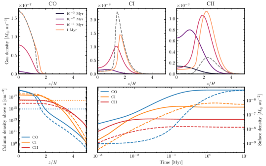
Figure 13: Same as Figure 4, but for $T=500$ K instead of 50 K, $\dot{M}_{+}=1$ $M_{\oplus}$ Myr^-1, $\alpha=10^{-2}$ and no vertical diffusion. The grey dashed lines in the top panels show the steady state gas density when $T=50$ K and scaled by a factor $1/\sqrt{10}$ for comparison. Similarly, the dashed coloured lines in the bottom left and right panels show the steady state column density profiles and the surface density evolution for $T=50$ K.

4.9 Limitations

The model presented here provides a useful tool to estimate and quantify the importance of vertical diffusion on the evolution of CO in exocometary discs. This model, nevertheless, has some limitations which we discuss here.

First, our model assumes that CO gas is released with a vertical profile that matches the hydrostatic equilibrium. In reality, the release of gas will depend on the vertical distribution of solids that dominate the gas release. If CO gas was released with a high vertical dispersion, the upper layers would be enriched in CO compared to our model. Therefore, shielding by carbon would be less effective. Conversely, if CO was released with a small vertical dispersion, it would be better shielded by CI. Moreover, we assumed a constant temperature. The temperature could vary as a function of height (reaching hundreds or thousands of K at the disc surface, Kral et al., 2019) or time as the gas densities and composition change (Kral et al., 2016). Both effects could have an impact on the level of mixing and thus on the gas evolution if they changed the ratio of the vertical diffusion and viscous timescales as discussed in §4.8. Exploring these scenarios would require solving the Navier-Stokes equations together with radiative transfer equations. Such demanding computations go beyond the scope of this paper. Additionally, the uncertainty would remain over how $\alpha$ and $\alpha_{\rm v}$ vary as a function of the temperature, density and ionization fraction (§4.3).

Second, our model is one dimensional and thus we cannot track the radial evolution of the gas. To approximate the viscous evolution, we remove gas on a viscous timescale at all heights. This might not necessarily be the case if the viscosity is height dependant. Nevertheless, this approximation provides a simple way to remove gas on a certain timescale. Moreover, our model is only strictly valid at the center of the belt, where CO gas is being released and there is negligible inflow of gas from another region. To model the gas interior or exterior to the belt, we would need to know the composition with which it arrives at that radius. Future modelling could solve self-consistently the radial and vertical evolution, allowing to study in more detail this evolution.

5 Conclusions

In this paper we have studied for the first time the vertical evolution of gas in debris discs, focusing on how the vertical distribution of carbon strongly affects the photodissociating radiation that CO receives. To this end, we developed a new 1D model and python package (exogas) that contains a module to simulate the vertical evolution of gas (in addition to a module to simulate the radial evolution as in Marino et al. 2020). Our model takes into account the release of CO gas from solids in a planetesimal belt, the photodissociation of CO, the ionisation/recombination of carbon, the radial viscous evolution, and the vertical mixing due to turbulent diffusion. Below we summarise our main findings.

First, we determined the efficiency of shielding by CI in two extreme hypothetical scenarios and confirmed previous findings. If carbon is primarily located in the surface layer below and above the CO gas, the lifetime of CO increases exponentially with the column density of CI (as argued by Kral et al., 2019). However, if CI and CO are vertically well mixed, shielding by CI is inefficient (Cataldi et al., 2020) and the CO lifetime increases only linearly with the CI column density. This demonstrates the importance of knowing the true vertical distribution of gas in debris discs to understand its evolution.

In order to understand what the true vertical distribution should be, we developed a 1D model to simulate the gas evolution. We showed for the first time how ISRF photodissociating radiation creates a surface layer dominated by atomic carbon and oxygen if gas densities are high and vertical diffusion is negligible. This surface layer acts as an efficient shield, where CI atoms absorb most of the interstellar UV photons and become ionised. This process creates three layers where carbon is in different forms: a top layer dominated by CII where the recombination rate is slow compared to ionisation, a surface or middle layer dominated by CI where recombination is efficient and where most UV radiation is absorbed, and a bottom layer that extends to the midplane and is dominated by CO. This layered structure allows the build up of a CO-rich midplane. However, if diffusion is strong CI and CO become well mixed, exposing CO to a stronger UV radiation. In this case, shielding by CI is inefficient and thus higher gas release rates would be required to achieve the same CO gas surface densities than with a weak vertical diffusion.

Since the strength of the turbulent diffusion ($\alpha_{\rm v}$) is uncertain in debris discs, we explored a wide range of values to characterise the different behaviours. We found that in steady state the vertical structure of the gas is mainly set by the vertical diffusion timescale ($H^{2}/D$) relative to the viscous timescale (i.e. the gas removal/replenishment timescale, $r^{2}/\nu$). In other words, if $\alpha_{\rm v}/\alpha>(H/r)^{2}$ diffusion happens faster than the gas replenishment and thus CO and CI are well mixed. Conversely, if $\alpha_{\rm v}/\alpha<(H/r)^{2}$ diffusion plays a minor role and a surface layer forms that is dominated by CI and oxygen, which shields the CO underneath. If the vertical diffusion timescale is longer than the age of the system, the CI gas could still form a surface layer if it is optically thick. Note that if gas densities are low enough such that the gas is optically thin to UV radiation in the vertical direction, CI and CO have very similar distributions independently of the diffusion strength.

Based on our results, we discussed what these findings imply for the known gas-rich debris discs. If diffusion is weak, the simple secondary scenario could still explain the population of gas-rich debris discs and account for the estimated CI masses. However, if observations of gas-rich debris discs indicate that CI and CO are well mixed, the standard secondary origin scenario might need reevaluation. Unfortunately, the strength of vertical diffusion in debris discs is unknown. If turbulence is driven by the MRI, $\alpha_{v}$ might be similar to $\alpha$ which would result in a well-mixed CO and CI gas. However, this picture could be even more complicated since we find that the ionisation varies greatly with height, which could make any MRI-driven diffusion height dependent.

We also discussed how turbulent diffusion could affect the vertical distribution of small grains. Those grains are susceptible to gas drag that damps their inclinations and thus should settle towards the midplane (Olofsson et al., 2022). However, turbulent diffusion can counterbalance this effect and limit the amount of settling. Measurements of the gas and small dust heights could provide constraints to the strength of vertical diffusion.

Whilst our simulations focused on the gas evolution at the belt centre, we showed how the efficiency of shielding has an effect on the viscous radial evolution of CO. Using radial evolution simulations we showed that if CO and CI are well mixed (and thus shielding by CI is weak) the CO lifetime might not be long enough for it to spread interior to the planetesimal belt. Therefore, the vertical evolution of the gas can have a profound effect on the radial distribution of CO.

Although vertical diffusion is largely unconstrained, using our simulations and radiative transfer predictions we showed that high-resolution ALMA observations could reveal if CO and CI are well mixed or segregated into different layers. Such observations would constrain $\alpha_{\rm v}/\alpha$ and ultimately determine how efficient shielding by CI is. This could confirm the exocometary origin of the gas, or favour a primordial origin where shielding is mostly done by hydrogen.

Finally, we discussed how attempts to infer the gas scale height directly from observations could suffer from large systematic errors. This is because the vertical distribution of CO and CI can be significantly different from the total gas distribution in gas-rich discs. CO gas can be concentrated towards the midplane, while CI can have an effective scale height much larger than the true value. We thus recommend the use of multiple species and the comparison with models as the one presented in this paper.

Data availability

The data underlying this article will be shared on reasonable request to the corresponding author. exogas can be downloaded from https://github.com/SebaMarino/exogas, where readers can also find examples of how to use it. disc2radmc can be downloaded from https://github.com/SebaMarino/disc2radmc, where examples are also available.

Appendix A Parameters

In Table 1 we summarise the most important parameters that we use.

Table 1: Model parameters, their default units, and description.

Parameter Unit Description $r$ au Planetesimal belt radius. $\Delta r$ au Full-width-half-maximum of planetesimal belt. $z$ au Height above the disc midplane. $H$ au Vertical disc scale-height as defined in Eq. 5. $\Sigma$ $M_{\oplus}$ au^-2 Total surface density of gas. $\rho(z)$ $M_{\oplus}$ au^-3 Total density of gas at height $z$. $\rho_{i}(z)$ $M_{\oplus}$ au^-3 Density of species $i$ (CO, CI or CII gas) at height $z$. $\Omega_{\rm K}$ rad yr^-1 Keplerian frequency. $c_{\rm s}$ m s^-1 Isothermal sound speed as defined in Eq. 6. $\mu$ … Mean molecular weight. $m_{\rm p}$ kg Proton mass. $L_{\star}$ $L_{\odot}$ Stellar luminosity. $T$ K Gas temperature as defined in Eq. 7. $\lambda$ nm Wavelength. $\theta$ rad Polar angle measured from the vertical direction. $\sigma_{\rm ph}(\lambda)$ cm² CO photodissociation cross section from Heays et al. (2017). $\sigma_{\rm CI}$ cm² CI ionisation cross section from Heays et al. (2017). $\sigma_{i}(\lambda)$ cm² cross section of species $i$. $\phi_{\lambda}$ s^-1 cm^-2 nm^-1 Interstellar radiation field from Draine (1978) with extension from van Dishoeck & Black (1982). $\tau_{i}(\lambda,\theta,z)$ … Optical depth of species i in the direction $\theta$ at height $z$ and wavelength $\lambda$ as defined in Eq. 12. $R_{\rm ph,0}$ yr^-1 Unshielded CO photodissociation rate per molecule as defined in Eq. 9. $R_{\rm ph}(z)$ yr^-1 CO Photodissociation rate per molecule at height z as defined in Eq. 10. $K(N_{\rm CO})$ … Shielding factor due to CO self-shielding as defined in Eq. 16. $\dot{\rho}_{\rm ph}(z)$ $M_{\oplus}$ au^-3 yr^-1 CO Photodissociation rate per unit volume at height $z$ as defined in Eq. 18. $R_{\rm ion,0}$ yr^-1 Ionisation rate per CI atom in the optically thin regime as defined in Eq. 20. $R_{\rm ion}(z)$ yr^-1 Ionisation rate per CI atom as defined in Eq. 19. $R_{\rm rc}(z)$ yr^-1 Recombination rate per CII atom as defined in Eq. 21. $\alpha_{\rm rc}(T)$ au³ yr^-1 Recombination rate coefficient. $n_{\rm e^{-}}(z)$ au^-3 Electron number density. $\dot{\rho}_{\rm ion}(z)$ $M_{\oplus}$ au^-3 yr^-1 Net ionisation rate per unit volume at height $z$ as defined in Eq. 22. $\dot{\rho}^{+}$ $M_{\oplus}$ au^-3 yr^-1 CO gas release rate per unit volume as defined in Eq. 4. $\dot{\Sigma}^{+}$ $M_{\oplus}$ au^-2 yr^-1 CO gas release rate per unit surface as defined in Eq. 8. $\dot{M}^{+}$ $M_{\oplus}$ yr^-1 CO gas release rate. $\dot{\rho}_{\rm vis,i}(z)$ $M_{\oplus}$ au^-3 yr^-1 Mass loss due to viscous evolution as defined in Eq. 23 $t_{\rm vis}$ yr Viscous timescale as defined in Eq. 24. $t_{\rm diff}$ yr Vertical diffusion timescale as defined in Eq. 27. $\nu$ au² yr^-1 Kinematic viscosity defined as $\alpha c_{\rm s}H$. $\alpha$ … Dimensionless viscosity parameter. $D$ au² yr^-1 Diffusion coefficient defined as $\alpha_{\rm v}c_{\rm s}H$. $\alpha_{\rm v}$ … Dimensionless vertical diffusion parameter. $\dot{\rho}_{i,D}$ $M_{\oplus}$ au^-3 yr^-1 Diffusion term as defined in Eq. 25.

Appendix B Vertical structure with $\alpha=10^{-1}$

In Figure 14 we show the vertical distribution of CO and CI as a function of the steady state surface density of gas, and for three different values of $\alpha_{\rm v}$: $10^{-4}$, $10^{-3}$, and $10^{-2}$. These correspond to the same ratios of $\alpha_{\rm v}/\alpha$ than those shown in §3.3. This demonstrates how the vertical distribution of CO and C will mostly depend on $\alpha_{\rm v}/\alpha$ rather than their absolute values.

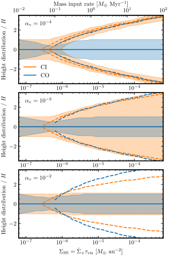
Figure 14: Vertical distribution in steady state of CO (blue) and CI (orange) normalized by the scale height ($H$) as a function of the steady state surface density of gas, in a case with $\alpha=10^{-1}$. The solid line shows where the density distribution peaks, while the shaded region represents the region where the density is at least 60% of the peak density ($1\sigma$ drop). The dashed lines represent the height at which CI and CO become optically thick to photodissociating radiation in the vertical direction. The top, middle, and bottom panels show scenarios where $\alpha_{\rm v}$ is $10^{-4}$, $10^{-3}$, and $10^{-2}$, respectively. The upper x-axis in the top panel shows the mass input rates as reference.

References

- Armitage (2011) Armitage P. J., 2011, ARA&A, 49, 195
- Badnell (2006) Badnell N. R., 2006, ApJS, 167, 334
- Casassus & Pérez (2019) Casassus S., Pérez S., 2019, ApJ, 883, L41
- Cataldi et al. (2020) Cataldi G., et al., 2020, ApJ, 892, 99
- Delage et al. (2021) Delage T. N., Okuzumi S., Flock M., Pinilla P., Dzyurkevich N., 2021, arXiv e-prints, p. arXiv:2110.05639
- Dent et al. (2014) Dent W. R. F., et al., 2014, Science, 343, 1490
- Draine (1978) Draine B. T., 1978, ApJS, 36, 595
- Flaherty et al. (2018) Flaherty K. M., Hughes A. M., Teague R., Simon J. B., Andrews S. M., Wilner D. J., 2018, ApJ, 856, 117
- Flaherty et al. (2020) Flaherty K., et al., 2020, ApJ, 895, 109
- Flock et al. (2015) Flock M., Ruge J. P., Dzyurkevich N., Henning T., Klahr H., Wolf S., 2015, A&A, 574, A68
- Fromang & Papaloizou (2006) Fromang S., Papaloizou J., 2006, A&A, 452, 751
- Gammie (1996) Gammie C. F., 1996, ApJ, 457, 355
- Greaves et al. (2016) Greaves J. S., et al., 2016, MNRAS, 461, 3910
- Heays et al. (2017) Heays A. N., Bosman A. D., van Dishoeck E. F., 2017, A&A, 602, A105
- Higuchi et al. (2019) Higuchi A. E., et al., 2019, ApJ, 883, 180
- Hughes et al. (2017) Hughes A. M., et al., 2017, ApJ, 839, 86
- Hughes et al. (2018) Hughes A. M., Duchêne G., Matthews B. C., 2018, ARA&A, 56, 541
- Igea & Glassgold (1999) Igea J., Glassgold A. E., 1999, ApJ, 518, 848
- Iglesias et al. (2018) Iglesias D., et al., 2018, MNRAS, 480, 488
- Ilgner & Nelson (2006) Ilgner M., Nelson R. P., 2006, A&A, 445, 223
- Izquierdo et al. (2021) Izquierdo A. F., Testi L., Facchini S., Rosotti G. P., van Dishoeck E. F., 2021, A&A, 650, A179
- Kama et al. (2016) Kama M., et al., 2016, A&A, 592, A83
- Kennedy (2018) Kennedy G. M., 2018, MNRAS, 479, 1997
- Klusmeyer et al. (2021) Klusmeyer J., et al., 2021, ApJ, 921, 56
- Kóspál et al. (2013) Kóspál Á., et al., 2013, ApJ, 776, 77
- Kral & Latter (2016) Kral Q., Latter H., 2016, MNRAS, 461, 1614
- Kral et al. (2016) Kral Q., Wyatt M., Carswell R. F., Pringle J. E., Matrà L., Juhász A., 2016, MNRAS, 461, 845
- Kral et al. (2019) Kral Q., Marino S., Wyatt M. C., Kama M., Matrà L., 2019, MNRAS, 489, 3670
- Kral et al. (2020a) Kral Q., Davoult J., Charnay B., 2020a, Nature Astronomy, 4, 769
- Kral et al. (2020b) Kral Q., Matrà L., Kennedy G. M., Marino S., Wyatt M. C., 2020b, MNRAS, 497, 2811
- Kral et al. (2021) Kral Q., et al., 2021, A&A, 653, L11
- Krivov et al. (2009) Krivov A. V., Herrmann F., Brandeker A., Thébault P., 2009, A&A, 507, 1503
- Lyra & Kuchner (2013) Lyra W., Kuchner M., 2013, Nature, 499, 184
- MacGregor et al. (2018) MacGregor M. A., et al., 2018, ApJ, 869, 75
- Marino (2022) Marino S., 2022, arXiv e-prints, p. arXiv:2202.03053
- Marino et al. (2016) Marino S., et al., 2016, MNRAS, 460, 2933
- Marino et al. (2018) Marino S., et al., 2018, MNRAS, 479, 5423
- Marino et al. (2020) Marino S., Flock M., Henning T., Kral Q., Matrà L., Wyatt M. C., 2020, MNRAS, 492, 4409
- Matrà et al. (2015) Matrà L., Panić O., Wyatt M. C., Dent W. R. F., 2015, MNRAS, 447, 3936
- Matrà et al. (2017) Matrà L., et al., 2017, ApJ, 842, 9
- Matrà et al. (2018) Matrà L., Wilner D. J., Öberg K. I., Andrews S. M., Loomis R. A., Wyatt M. C., Dent W. R. F., 2018, ApJ, 853, 147
- Matrà et al. (2019) Matrà L., Öberg K. I., Wilner D. J., Olofsson J., Bayo A., 2019, AJ, 157, 117
- Montgomery & Welsh (2012) Montgomery S. L., Welsh B. Y., 2012, PASP, 124, 1042
- Moór et al. (2017) Moór A., et al., 2017, ApJ, 849, 123
- Moór et al. (2019) Moór A., et al., 2019, ApJ, 884, 108
- Nakatani et al. (2021) Nakatani R., Kobayashi H., Kuiper R., Nomura H., Aikawa Y., 2021, ApJ, 915, 90
- Öberg et al. (2015) Öberg K. I., Guzmán V. V., Furuya K., Qi C., Aikawa Y., Andrews S. M., Loomis R., Wilner D. J., 2015, Nature, 520, 198
- Okuzumi & Hirose (2011) Okuzumi S., Hirose S., 2011, ApJ, 742, 65
- Olofsson et al. (2022) Olofsson J., et al., 2022, arXiv e-prints, p. arXiv:2202.08313
- Pearce et al. (2020) Pearce T. D., Krivov A. V., Booth M., 2020, MNRAS, 498, 2798
- Pinte et al. (2016) Pinte C., Dent W. R. F., Ménard F., Hales A., Hill T., Cortes P., de Gregorio-Monsalvo I., 2016, ApJ, 816, 25
- Pinte et al. (2018) Pinte C., et al., 2018, A&A, 609, A47
- Rebollido et al. (2018) Rebollido I., et al., 2018, A&A, 614, A3
- Rebollido et al. (2020) Rebollido I., et al., 2020, A&A, 639, A11
- Rollins & Rawlings (2012) Rollins R. P., Rawlings J. M. C., 2012, MNRAS, 427, 2328
- Shakura & Sunyaev (1973) Shakura N. I., Sunyaev R. A., 1973, A&A, 24, 337
- Slettebak (1975) Slettebak A., 1975, ApJ, 197, 137
- Smirnov-Pinchukov et al. (2021) Smirnov-Pinchukov G. V., Moór A., Semenov D. A., Ábrahám P., Henning T., Kóspál Á., Hughes A. M., Folco E. d., 2021, MNRAS,
- Stoll et al. (2017) Stoll M. H. R., Kley W., Picogna G., 2017, A&A, 599, L6
- Takeuchi & Artymowicz (2001) Takeuchi T., Artymowicz P., 2001, ApJ, 557, 990
- Teague et al. (2018) Teague R., Bae J., Bergin E. A., Birnstiel T., Foreman-Mackey D., 2018, ApJ, 860, L12
- Thébault & Augereau (2005) Thébault P., Augereau J. C., 2005, A&A, 437, 141
- Van Clepper et al. (2022) Van Clepper E., Bergner J. B., Bosman A. D., Bergin E., Ciesla F. J., 2022, arXiv e-prints, p. arXiv:2202.00524
- Visser et al. (2009) Visser R., van Dishoeck E. F., Black J. H., 2009, A&A, 503, 323
- Wyatt (2008) Wyatt M. C., 2008, ARA&A, 46, 339
- Wyatt et al. (2007) Wyatt M. C., Smith R., Greaves J. S., Beichman C. A., Bryden G., Lisse C. M., 2007, ApJ, 658, 569
- Xu et al. (2017) Xu Z., Bai X.-N., Murray-Clay R. A., 2017, ApJ, 847, 52
- Youdin & Lithwick (2007) Youdin A. N., Lithwick Y., 2007, Icarus, 192, 588
- Youngblood et al. (2021) Youngblood A., Roberge A., MacGregor M. A., Brandeker A., Weinberger A. J., Pérez S., Grady C., Welsh B., 2021, AJ, 162, 235
- Zhu et al. (2015) Zhu Z., Stone J. M., Bai X.-N., 2015, ApJ, 801, 81
- Zuckerman & Song (2012) Zuckerman B., Song I., 2012, ApJ, 758, 77
- Zuckerman et al. (1995) Zuckerman B., Forveille T., Kastner J. H., 1995, Nature, 373, 494
- van Dishoeck & Black (1982) van Dishoeck E. F., Black J. H., 1982, ApJ, 258, 533