Conformally coupled theories and their deformed compact objects:
from black holes, radiating spacetimes to eternal wormholes

Abstract

We study a higher order conformally coupled scalar tensor theory endowed with a covariant geometric constraint relating the scalar curvature with the Gauss-Bonnet scalar. It is a particular Horndeski theory including a canonical kinetic term but without shift or parity symmetry for the scalar. The theory also stems from a Kaluza-Klein reduction of a well defined higher dimensional metric theory. Properties of an asymptotically flat spherically symmetric black hole are analyzed, and new slowly rotating and radiating extensions are found. Through disformal transformations of the static configurations, gravitating monopole-like solutions and eternal wormholes are presented. The latter are shown to extract from spacetime possible naked singularities, yielding completely regular and asymptotically flat spacetimes.

I Introduction

In recent years, scientific interest and research in black holes, neutron stars and other more exotic compact objects, such as wormholes Morris:1988cz , has increased considerably. This is largely due to the plethora of recent astrophysical observations LIGOScientific:2017vwq ; LIGOScientific:2020zkf ; LIGOScientific:2021qlt which confirm or re-affirm, the existence of compact objects as well as their defining properties. These observations are in their vast majority in accordance with General Relativity (GR) at their current accuracy. Certain unexpected results do emerge however, questioning certain standard expectations from GR. For example, the recent observation of the compact object merger GW190814 LIGOScientific:2020zkf where the secondary compact object has a mass of $2.59_{-0.09}^{+0.08}~{}M_{\odot}$, placing it in the mass gap in-between neutron stars and black holes for GR. From classical GR results such as Buchdahl limit on compacity, such a compact object of astrophysical origin could be explained only as a neutron star with an unexpectedly stiff (or exotic) EOS (quite incompatible with GW170817), a neutron star with a too rapid rotation, or a black hole with a small mass whose origin is difficult to explain (for a discussion see Charmousis:2021npl and references within).

It is clear that we are entering a novel era in gravitational observations, and technological/observational advances in the near future will definitely bring to light new aspects of gravitational physics, some of which probably not anticipated, that we will still have to comprehend. We are presented therefore with quite a challenge in gravitational theory with the need to extend our understanding concerning the existence and properties of compact objects as solutions of GR or other theories of gravity. It is also important to emphasize that although most current observational data are in agreement with the theory of GR, this should in no way prevent us from exploiting alternative gravity theories as they provide a measurable ruler of departure from classical relativity theory. In this perspective, it is certain that the emergence of new gravitational solutions (associated with modified theories) will enrich our understanding of recent and future observations. Therefore, it is crucial to search for modifications of GR and to explore new promising theoretical possibilities in theories of gravity. In order to carry out this project, we must specify our modified theories of gravity so that they are physically acceptable while also ensuring the existence of analytical solutions, which are an important condition for making accurate comparison of GR and its modifications using observations.

Modifications of gravity can be realized with increasingly complex formulations but, in the present case, we will be restricting ourselves to scalar-tensor theories which are the simplest, working, robust prototype of modified gravity theories with a single additional degree of freedom. They also appear as a limit of most modified gravity theories however complex their nature. In recent years, higher order scalar tensor theories (with second-order field equations) have been rediscovered, and intensively studied highlighting the precursor work of Horndeski Horndeski:1974wa from the seventies. For latter convenience, we specify the Horndeski action which is nothing but the most general (single) scalar-tensor theory with second order equations of motion,

$$S=\int\mathrm{d}^{4}x\sqrt{-g}\,\Big{\{}\mathcal{L}_{2}+\mathcal{L}_{3}+\mathcal{L}_{4}+\mathcal{L}_{5}\Big{\}},$$ (1)

with

$$\mathcal{L}_{2}=G_{2},\quad\mathcal{L}_{3}=-G_{3}\Box\phi,\quad\mathcal{L}_{4}=G_{4}R+G_{4X}\left[\left(\Box\phi\right)^{2}-\left(\phi_{\mu\nu}\right)^{2}\right],$$

$$\mathcal{L}_{5}=G_{5}\,G_{\mu\nu}\phi^{\mu\nu}-\frac{1}{6}G_{5X}\left(\left(\Box\phi\right)^{3}-3\Box\phi\left(\phi_{\mu\nu}\right)^{2}+2\phi_{\mu\nu}\phi^{\nu\rho}\phi{{}^{\mu}_{\rho}}\right),$$

where $\phi_{\mu}=\nabla_{\mu}\phi$, $\phi_{\mu\nu}=\nabla_{\mu}\nabla_{\nu}\phi$, and the $G_{k}$’s are arbitrary functions of $\phi$ and of the standard kinetic term $X=-\phi_{\mu}\phi^{\mu}/2$ parametrising the Horndeski theory.

Sectors of the Horndeski theory and beyond have been exploited in the current literature (see Babichev:2013cya ; BenAchour:2019fdf ; Babichev:2017guv and references therein) providing explicit compact object solutions and related results. As it turns out, the theories which allow analytic construction of solutions are, mostly restricted to a shift-symmetric and parity-preserving scalar field. The shift-symmetry of the scalar field yields a Noether conserved current which proves extremely useful for integrating the equations of motion. The lesson to be learned from these examples is that symmetries underlying the action of the scalar tensor theories (1) are key in obtaining workable analytic solutions. From this observation, it is natural to focus in the classes of Horndeski theories possessing symmetries simplifying the equations of motion. Such a symmetry could also be the conformal invariance of the equation of motion of the scalar field. The advantage of the latter is the existence of a covariant purely geometric constraint which does not involve the scalar field. This idea is not new and finds its origin in the first counter-example to the no-hair theorem with the discovery of the so-called BBMB black hole Bocharova:1970skc ; Bekenstein:1974sf which corresponds to a static solution of the Einstein equations with a conformally coupled scalar field in four dimensions. In this case, the purely geometric equation which allows the integration of the equations of motion is the vanishing Ricci scalar, $R=0$. In presence of a cosmological constant with a self-interacting potential, this constraint is modified to $R=\mbox{cst}$, while conformal invariance for the scalar is not spoilt. As a result analytic black hole solutions of de Sitter and anti de Sitter asymptotics were found in Martinez:2002ru ; Martinez:2005di . Quite recently this approach was nicely extended to the most general (higher order) Horndeski action with a conformally-invariant scalar field equation Fernandes:2021dsb ,

$$S=\int\mathrm{d}^{4}x\frac{\sqrt{-g}}{16\pi}\left\{R-2\lambda e^{4\phi}-\beta\mathrm{e}^{2\phi}\left(R+6\left(\nabla\phi\right)^{2}\right)-\alpha\left[\phi\mathcal{G}-4G^{\mu\nu}\phi_{\mu}\phi_{\nu}-4\Box\phi\left(\nabla\phi\right)^{2}-2\left(\nabla\phi\right)^{4}\right]\right\},$$ (2)

and, cerise sur le gâteau, this action belongs to a non-shift symmmetric Horndeski class (1) without parity symmetry. Indeed all the Horndeski coupling functions are present taking the form,

$$G_{2}=-2\lambda e^{4\phi}+12\beta e^{2\phi}X+8\alpha X^{2},\quad G_{3}=8\alpha X,\quad G_{4}=1-\beta e^{2\phi}+4\alpha X,\quad G_{5}=4\alpha\ln\left\lvert X\right\rvert.$$ (3)

Here $\alpha$, $\beta$ and $\lambda$ are constant parameters and $\mathcal{G}=R^{2}-4R_{\mu\nu}R^{\mu\nu}+R_{\mu\nu\rho\sigma}R^{\mu\nu\rho\sigma}$ is the Gauss-Bonnet scalar, while a cosmological constant may also be added to the action (2). The particularity of the construction in Fernandes:2021dsb however, is that the trace of the metric equations together with the scalar field equation associated to the action (2) combine to give a purely geometric four-dimensional equation,

$$R+\frac{\alpha}{2}\mathcal{G}=0.$$ (4)

With the help of this geometric constraint, two analytic static solutions, with nontrivial scalar fields, were presented in Fernandes:2021dsb , for $\beta\neq 0$. In fact, each of them exists for a precise tuning between the coupling constants $\alpha$, $\beta$ and $\lambda$ in action (2), so the associated theories are distinct. We will focus on one of these solutions and its corresponding theory, which presents the attractive feature of both a canonical kinetic term and a well-defined scalar field in the whole spacetime (minus the origin). Last but not least, the latter solution also has a higher dimensional origin. Indeed it is interesting to note that the above action (3) can be approached from an alternative route involving the Kaluza-Klein compactification of $D-$dimensional Einstein-Gauss-Bonnet theory Kiritsis . There it was shown that starting from a $D>4$ dimensional solution of Lovelock gravity with a non trivial horizon Dotti:2005rc ; Bogdanos , one can construct a scalar tensor black hole solution in four dimensions Kiritsis . These solutions, due to their higher dimensional origin, do not have a standard four dimensional Newtonian mass term. Crucially however, upon taking a singular limit (as first considered by Glavan ), action (2) and the latter solution from Fernandes:2021dsb , can be obtained from Kiritsis with a standard four dimensional mass term.

We thus provide a detailed analysis of this solution in the first part of the present work, by studying the nature of the singularities, depending on the sign of the coupling constant $\alpha$. Indeed, we show that the case $\alpha>0$ is well-behaved, with a spacetime defined in the whole region $r>0$, and with a singularity at $r=0$ always hidden by a horizon, while for $\alpha<0$, a naked singularity may appear. Then, starting from the observation that the solutions of Fernandes:2021dsb do not reduce to flat spacetime, we seek non-trivial flat spacetime solutions of the given theory. We present two classes of flat spacetime solutions with a non trivial time-dependent scalar field. We furthermore extend the solution of Fernandes:2021dsb to find a slowly rotating black hole solution, as well as a radiating/accreting Vaidya-like solution for this modified gravity theory.

Another aspect that has been recently studied in the literature for (beyond) Horndeski theories has to do with disformal transformations of the metric, see Ref. Zumalacarregui:2013pma . Starting from a seed solution given by a scalar field $\phi$ and a metric $g$ of a given Horndeski theory, the deformed metric $\tilde{g}_{\mu\nu}=g_{\mu\nu}+D(\phi,X)\partial_{\mu}\phi\partial_{\nu}\phi$ solves a beyond Horndeski theory, along with an unchanged scalar field. Disformal transformations are very useful in engineering solutions with highly non-trivial properties from simpler seed solutions. In particular, in Ref. Anson:2020trg , disformal versions of the Kerr spacetime with a regular scalar field were explicitly constructed and analyzed starting from a stealth Kerr solution Charmousis:2019vnf . Such rotating black holes have particular non-GR observational signatures Anson:2021yli , which in the near future may be probed and contrasted with the Kerr solution. Disformal transformations can also give rise to explicit asymptotically flat wormhole solutions Bakopoulos:2021liw (see also Faraoni:2021gdl , Chatzifotis:2021hpg and also Kanti:2011jz for earlier works). We will exploit this direction in the second part of the paper to construct regular wormholes and regular monopole-like solutions.

In the next section, we will analyze the black holes in question, portraying non trivial flat spacetime solutions as well as their slowly rotating and Vaidya like counterparts. We will then in the third section discuss ways to circumvent certain shortcomings of the initial solution portraying in particular eternal wormhole metrics as well as regular monopole-like solutions. We will conclude our analysis discussing future prospects. For clarity, we will include slowly rotating and radiating extensions of other solutions to action (2), as well as the specific disformed theories of the latter action, in the appendix.

II A hairy black hole solution, its flat counterpart and generalizations

II.1 Black hole analysis

The theory under consideration (2) presents several noteworthy properties. For a start, it is the most general scalar-tensor action with second-order equations of motion endowed with a conformally coupled scalar field Fernandes:2021dsb . Secondly, action (2) has a higher dimensional origin from a purely metric theory, namely Lovelock theory Lovelock:1971yv (see Charmousis:2008kc for a review). In effect, the conformally coupled theory can be also obtained in a two step fashion: from a consistent Kaluza-Klein reduction of higher dimensional Lovelock theory Kiritsis where the dimension $D$ is a continuous parameter, followed by a singular limit of $D\rightarrow 4$ as first considered in Glavan , and later applied in this context in Lu:2020iav . A third important fact is the presence, when $\beta\neq 0$, of a canonical kinetic term (obtained by a simple field redefinition $\Phi=\mathrm{exp}\left(\phi\right)$), and the absence of shift or parity symmetry. As a direct consequence, this theory is not subject to the standard shift symmetric Horndeski no hair theorem Hui:2012qt , and hence it is not clear a priori which properties compact solutions of (2) may acquire. In fact, in a recent elegant paper Fernandes:2021dsb , the author finds distinct classes of static solutions for the scalar tensor theory (2) with a particular tuning in between the coupling constants $\lambda$, $\beta$ and $\alpha$ (see also Lu:2020iav , Fernandes:2022zrq and references within). Different cases, along with new solutions, will be discussed in the appendices, but in the main body of the paper, we will focus on the unique solution of Fernandes:2021dsb with both $\beta\neq 0$ and a scalar field with a logarithmic behavior which is well defined everywhere but the origin, and the couplings satisfying the constraint $\lambda=\frac{\beta^{2}}{4\alpha}$. This latter is given by

$$\mathrm{d}s^{2}=-f(r)\mathrm{d}t^{2}+\frac{\mathrm{d}r^{2}}{f(r)}+r^{2}\left(\mathrm{d}\theta^{2}+\sin^{2}\theta\,\mathrm{d}\varphi^{2}\right),$$ (5)

with

$$f(r)=1+\frac{r^{2}}{2\alpha}\left(1-\sqrt{1+8\alpha\left(\frac{M}{r^{3}}+\frac{\alpha}{r^{4}}\right)}\right)$$ (6)

and

$$\phi=\phi(r)=\ln\left(\frac{\sqrt{-2\alpha/\beta}}{r}\right).$$ (7)

The solution depends on a unique integration constant denoted by $M$ (and corresponding to the mass, as proven below), and exists provided the couplings $\alpha$ and $\beta$ are of opposite sign. It is therefore a black hole with secondary hair, as are most scalar-tensor black holes. However, note that the scalar charge of this solution is not trivial. Indeed, if we switch off the integration constant, $M=0$, we do not end up with flat spacetime, rather a singular solution at $r=0$ (with singularity covered by an event horizon for $\alpha>0$), and this is essentially due to the additional $\alpha^{2}/r^{4}$ term under the square root in (6). This latter term can be seen to be related to the scalar charge of the black hole. Note in fact that at $r=0$ the solution behaves as $f\left(r\right)\sim 1-\text{sign}\left(\alpha\right)\sqrt{2}+O(r)$ which is finite and certainly not equal to 1. This seemingly milder singularity is a true curvature singularity at $r=0$, in agreement with the logarithmically singular scalar field there. Therefore we see that the canonical kinetic term does come at the expense of a singular vacuum, therefore an essential question that will occupy us later on in this section is the existence of a flat solution in this theory.

For the moment, let us pursue the study of the spacetime (5). The spacetime for the solution exhibits very distinct properties depending on the sign of the coupling constant $\alpha$. For $\alpha<0$ (and hence $\beta>0$), the standard kinetic term has the usual sign in the action, and the coupling constant of the potential term $\lambda=\frac{\beta^{2}}{4\alpha}<0$. For convenience, we rewrite the spacetime (5) for the choice $\alpha<0$ as follows,

$$f\left(r\right)=1-\frac{r^{2}}{2\left|\alpha\right|}+\frac{\sqrt{P\left(r\right)}}{2\left|\alpha\right|},\quad P\left(r\right)\equiv r^{4}-8\left|\alpha\right|Mr+8\left|\alpha\right|^{2},$$ (8)

and we define the radius $r=r_{P}$ and the values $M_{\text{NS}}$ and $M_{\text{min}}$,

$$P\left(r_{P}\right)\equiv 0,\qquad\frac{\left|\alpha\right|}{M_{\text{NS}}^{2}}\equiv\frac{3}{4}\sqrt{\frac{3}{2}},\qquad\frac{\left|\alpha\right|}{M_{\text{min}}^{2}}\equiv\frac{8}{9}.$$ (9)

It is easy to see that for $0\leq M\leq M_{\text{NS}}$, the spacetime admits a naked singularity at $r=0$, while if $M_{\text{NS}}<M<M_{\text{min}}$, the naked singularity is brought forward to $r=r_{P}$. Only for larger masses $M\geq M_{\text{min}}$ (as compared to the coupling constant $\left\lvert\alpha\right\rvert$) does the spacetime describe a black hole with a single event horizon at $r_{+}=M+\sqrt{M^{2}-\left|\alpha\right|}$ covering the singularity at $r=r_{P}$. Note that for $\alpha<0$ the event horizon has smaller size compared to the standard Schwarzschild radius $r_{\text{Sch}}=2M$. In particular the minimal horizon size is $r_{+}^{\text{min}}=\sqrt{2|\alpha|}=\frac{4}{3}M_{\text{min}}$. The behavior of the metric function is illustrated in Fig. 1 (left panel), where $f\left(r\right)$ is shown for different $M/\sqrt{\left\lvert\alpha\right\rvert}$.

Figure 1: Metric function $f(r)$ for different values of $M/\sqrt{\left\lvert\alpha\right\rvert}$ for negative $\alpha$ (left plot) and positive $\alpha$ (right plot). On the left panel, for $M\leq M_{\text{NS}}$, the upper curves correspond to the spacetime with a naked singularity at $r=0$. For $M_{0}<M<M_{\text{min}}$, the spacetime has a naked singularity at $r=r_{P}$, while for $M\geq M_{\text{min}}$ the metric describes a black hole. On the right panel, the spacetime admits a singularity at $r=0$, always covered by the horizon.

For $\alpha<0$, the lower bound on the mass $M\geq M_{\text{min}}$ ensuring the existence of a black hole solution implies an upper bound on the value of the coupling parameter $\left|\alpha\right|$. Indeed, following Ref. Charmousis:2021npl , one can obtain a constraint on $\alpha$ using data on observed (candidates of) black holes. In the event GW$200115$, one component was certainly identified as a black hole of mass $M=5.7_{-2.1}^{+1.8}\,M_{\odot}$. This gives a constraint

$$\left|\alpha\right|\lesssim 253_{-152}^{+184}\,\mbox{km}^{2}.$$ (10)

If we include the events GW$170817$ and GW$190814$, we obtain stronger constrains, $\left|\alpha\right|\lesssim 59\,\mbox{km}^{2}$, and $\left|\alpha\right|\lesssim 52\,\mbox{km}^{2},$ correspondingly, however the presence of a black hole is only probable (but not certain) for these two events.

The case $\alpha>0$ is more straightforward to analyze since, independently of the value for $\alpha$, the solution (5) describes a black hole for any mass $M$, and with a unique horizon $r_{+}=M+\sqrt{M^{2}+\alpha}$ covering the singularity $r=0$. The horizon is now at $r_{+}>r_{\text{Sch}}=2M$. The behavior of the function $f(r)$ is illustrated in Fig. 1.

To conclude the discussion, we would like to mention, in the spirit of Charmousis:2021npl , that if a Birkhoff-like uniqueness theorem were valid for the solution (5-7), it would inevitably lead to the constraint $\alpha<0$. Indeed, if the solution (5) were unique, any static and spherically symmetric object of mass $M$ would create an exterior gravitational field given by (5). If $\alpha>0$, this object would therefore be a black hole with horizon $r_{+}=M+\sqrt{M^{2}+\alpha}$, unless this event horizon is hidden below the surface of the object. An atomic nucleus has radius $R\sim 10^{-15}\,\mbox{m}$, and is not a black hole since it can be experimentally probed, therefore $r_{+}<R$, yielding

$$0<\alpha<R\left(R-2M\right)\sim 10^{-30}\,\mbox{m}^{2},$$ (11)

essentially rendering $\alpha>0$ irrelevant.

II.2 Black hole thermodynamics

Let us now turn to the thermodynamic properties of the black holes of  (2). Since the theory in question descends from a spin $2$ metric Lovelock theory, its thermodynamic aspects can be quite intriguing Myers:1988ze , Clunan:2004tb . In particular, one may ask whether the one-quarter area law of the entropy is preserved or not. In order to give a clear answer we choose to use the Euclidean approach for a general class of spherically symmetric metrics parameterized as,

$$\mathrm{d}s_{\mbox{\tiny{Eucl}}}^{2}=N(r)^{2}f(r)\mathrm{d}\tau^{2}+\frac{\mathrm{d}r^{2}}{f(r)}+r^{2}\mathrm{d}\Omega^{2},$$ (12)

where $\tau$ is the Euclidean time. To avoid a conical singularity at the horizon, the Euclidean time is made periodic with period $1/T$, where $T$ is the Hawking temperature. Since we are interested in a static solution with a radial scalar field, we can restrict ourselves to a reduced action. The latter can be obtained by substituting the Euclidian metric (12) in the action (2) and performing several integrations by parts,

$$I_{E}=\int_{r_{+}}^{\infty}\text{d}r\left\{-\frac{N}{2T}\Big{[}r(1-\beta e^{2\phi})+\left(2\alpha(3f-1)-\beta r^{2}e^{2\phi}\right)\phi^{\prime}+6f\alpha r(\phi^{\prime})^{2}+2r^{2}\alpha(\phi^{\prime})^{3}f\Big{]}f^{\prime}\right.$$

$$-\frac{N}{2T}\Big{[}2f\left(2\alpha f-2\alpha-\beta r^{2}e^{2\phi}\right)+8\alpha f^{2}r\phi^{\prime}+4r^{2}\alpha f^{2}(\phi^{\prime})^{2}\Big{]}\phi^{\prime\prime}$$ (13)

$$-\frac{N}{2T}\left[-r^{2}\alpha f^{2}(\phi^{\prime})^{4}+\left(2\alpha f+2\alpha-\beta r^{2}e^{2\phi}\right)f(\phi^{\prime})^{2}-4\beta rfe^{2\phi}\phi^{\prime}-1+f+\beta e^{2\phi}(1-f)+\lambda r^{2}e^{4\phi}\right]\left.\right\}+B$$

Here, $B$ is a boundary term that is fixed by requiring that the solution of the equations of motion is an extremum of the Euclidean action. This condition implies that

$${\delta B}=\frac{N}{2T}\Big{[}r(1-\beta e^{2\phi})+\left(2\alpha(3f-1)-\beta r^{2}e^{2\phi}\right)\phi^{\prime}+6f\alpha r(\phi^{\prime})^{2}+2r^{2}\alpha(\phi^{\prime})^{3}f\Big{]}(\delta f)+\left[\cdots\right](\delta\phi^{\prime})+\left[\cdots\right](\delta\phi),$$ (14)

where the terms proportional to $(\delta\phi),(\delta\phi^{\prime})$ are omitted for simplicity as they vanish identically on-shell. It is worth noticing an interesting feature of the solution we consider here. In general, the boundary term depends on the parameter $\beta$, as can be seen from the above equation. However, on-shell the terms proportional to $\delta\phi$ and $\delta\phi^{\prime}$ drop out, while inside the first bracket, terms involving the $\beta$ parameter also cancel out. Therefore the resulting thermodynamic expression does not depend on $\beta$ for the solution (5)-(7), as we will see below. Indeed, on-shell the variation of the boundary term reduces to the following simple expression

$${\delta B}=\frac{1}{2Tr}\Big{[}2\alpha(1-f)+r^{2}\Big{]}(\delta f).$$ (15)

From the above expression it follows that

$$(\delta B)|_{\infty}=-\frac{1}{2T}\left(1+\frac{\alpha}{r_{+}^{2}}\right)(\delta r_{+})\quad\Longrightarrow\quad B|_{\infty}=-\frac{1}{2T}\left(r_{+}-\frac{\alpha}{r_{+}}\right)$$

while for the variation at the horizon,

$$(\delta B)|_{r_{+}}=-2\pi\left(r_{+}+\frac{2\alpha}{r_{+}}\right)(\delta r_{+})\quad\Longrightarrow\quad B|_{r_{+}}=-\pi\left[r_{+}^{2}+4\alpha\ln(r_{+})\right].$$

Hence, on-shell, the Euclidean action (II.2) has value

$$I_{E}=-\frac{1}{2T}\left(r_{+}-\frac{\alpha}{r_{+}}\right)+\left[\pi r_{+}^{2}+4\pi\alpha\ln(r_{+})\right].$$ (16)

Comparing the above expression with the relation of the Euclidean action to the mass ${\cal M}$ and the entropy ${\cal S}$ in the grand canonical ensemble, $I_{E}=-\frac{\cal M}{T}+{\cal S}$, we find that for the black hole solution (5)-(7),

$${\cal M}=\frac{1}{2}\left(r_{+}-\frac{\alpha}{r_{+}}\right)=M,\qquad{\cal S}=\pi r_{+}^{2}+4\pi\alpha\ln(r_{+}).$$ (17)

Hence, one concludes that the usual one-quarter area law of the entropy for general relativity is violated, as to be expected from standard results in Lovelock gravityMyers:1988ze . Nevertheless, the first law of thermodynamics holds, $d{\cal M}=Td{\cal S}$, with the Hawking temperature given by

$$T=\frac{r_{+}^{2}+\alpha}{4\pi r_{+}(2\alpha+r_{+}^{2})}.$$ (18)

As things stand we note that for $\alpha<0$, the temperature diverges, i.e. $T\to\infty$ as $M$ goes to the minimal mass of the black hole $M_{\text{min}}$. This is not a priori a problem, however, the free energy $F\equiv M-T\cal S$ then also diverges at a finite mass. This can be remedied noting that the entropy is defined up to a constant $s$, namely

$${\cal S}_{\alpha<0}=\pi\left(r_{+}^{2}-2\left\lvert\alpha\right\rvert\ln\frac{r_{+}^{2}}{s\left\lvert\alpha\right\rvert}\right).$$ (19)

We now fix $s=\frac{2}{\exp\left(1\right)}=\frac{2}{\rm e}$ to have vanishing entropy as $M\to M_{\text{min}}$ and therefore a finite free energy (similar to the case of a Schwarzschild black hole in GR). For this choice of $s$, the free energy is positive (see also Clunan:2004tb ) and finite for any mass, decreasing from $M$ to $M/2$ as $M$ runs from $M_{\text{min}}$ to $\infty$.

For positive $\alpha$ there is no lower limit on the black hole mass, and $T$ does not diverge for $M=0$. We can fix the free constant $s$ so that the entropy vanishes for the minimal mass $M=0$, resulting in

$${\cal S}_{\alpha>0}=\pi\left(r_{+}^{2}+2\alpha\ln\frac{r_{+}^{2}}{\rm{e}^{1/2}\alpha}\right).$$ (20)

For $\alpha>0$ the free energy increases from $0$ to $M/2$ as $M$ runs from $0$ to $\infty$. Let us finally mention that, as for the Schwarzschild black hole, the heat capacity is negative for any sign of $\alpha$.

II.3 A non trivial vacuum, the slowly rotating and Vaidya-like extensions

As we pointed out in the beginning of the section, the solution (5)-(7) does not reduce to flat spacetime in the limit of zero black hole mass, $M\to 0$. Moreover, as mentioned before, the zero mass spacetime has a singularity at $r=0$ which is either naked ($\alpha<0$) or covered by a horizon ($\alpha>0$). One can also show that a trivial scalar field does not lead to a flat spacetime solution. This means that any flat geometric vacuum will necessarily require a non trivial scalar field. Indeed, solving the field equations with a general $\phi=\phi(t,r)$ and a flat metric, i.e. Eq. (5) with $f=1$, we find two solutions, where the time-dependence of the scalar field must be non-trivial,

$$\phi(t)=\ln\left(\frac{\sqrt{\left(-2\alpha/\beta\right)\left(3\pm\sqrt{6}\right)}}{\left|t+\mu\right|}\right),\quad\phi(t,r)=\ln\left(\frac{\sqrt{\left(-8\mu\alpha/\beta\right)\left(3\pm\sqrt{6}\right)}}{\left|r^{2}-t^{2}+\mu\right|}\right),$$ (21)

and $\mu$ is an arbitrary constant. None of these profiles is differentiable in the whole spacetime. The solution (5)-(7) and the flat configurations presented above cannot be smoothly deformed into each other, which suggests that they belong to different, disconnected sectors. Similar solutions have been discussed for non minimally coupled scalar fields in Refs. Ayon-Beato:2005yoq and Ayon-Beato:2004nzi . In a somewhat different context, the so-called Fab 4 theory, non-trivial flat vacua exist with self-tuning properties Charmousis:2014mia , although there is no hint of self tuning within the presently considered theory.

It would be very interesting if one could generalize the static solution (5)-(7) to its stationary version. A fully analytic solution is not seemingly easily found, one can however, as a first step, find the slowly rotating solution in the manner described by Hartle and Thorne in GR Hartle:1967he ; Hartle:1968si . The Hartle-Thorne formalism in the presence of matter is very useful for calculating, for example, the moment of inertia for neutron stars. In particular, for most observed pulsars the Hartle-Thorne formalism is a good approximation of their gravitational field. Here, in the absence of matter, we will seek the slowly rotating version of our static solution.

For the slowly rotating solution, we start with an ansatz for the metric of the form

$$\mathrm{d}s^{2}=-f(r)\mathrm{d}t^{2}+\frac{\mathrm{d}r^{2}}{f(r)}+r^{2}\mathrm{d}\Omega^{2}-2\delta\,\omega(r)\,r^{2}\sin^{2}\theta\mathrm{d}t\mathrm{d}\varphi,$$ (22)

where $\delta$ is a first order parameter, such that the angular momentum per unit mass is given by $\delta a$ for slowly rotating solutions. At first order, the only new contribution in the equations of motion in comparison with the static case is the off-diagonal $t\varphi-$component, while the geometric constraint $R+\frac{\alpha}{2}\mathcal{G}=0$ is not affected at first order. As a direct consequence, one finds that the metric function $f(r)$ and the scalar field $\phi$ have the same profile (5)-(7) as in the static case, while the solution for $\omega\left(r\right)$ is

$$\omega(r)=-6aM\int_{\infty}^{r}\frac{\mathrm{d}r}{r^{4}\sqrt{1+8\alpha\left(\frac{M}{r^{3}}+\frac{\alpha}{r^{4}}\right)}}.$$ (23)

As $r\to\infty$, the integral gives to leading order the GR behavior, with $\delta J=\delta aM$ the total angular momentum,

$$\omega\left(r\right)=\frac{2J}{r^{3}}\left[1-\frac{2\alpha M}{r^{3}}-\frac{12\alpha^{2}}{7r^{4}}+\mathcal{O}\left(\frac{1}{r^{6}}\right)\right],$$

and higher order correction terms in $\alpha$. The variable $\omega$, as in GR, describes the speed at which a geodesic observer rotates because of frame dragging.

Yet another interesting feature of the static solution (5)-(7) within the action (2) is that it can be extended to a radiating (or absorbing) Vaidya-like solution. The Vaidya solution in GR describes a black hole with varying mass due to either radiation or accretion of pressureless light-like matter. It is relevant, as a paradigm for Hawking radiation or classically simulating gravitational collapse of null dust. In the case of GR, the recipe for the construction of the Vaidya solution is to use the retarded $u$ (or advanced $v$) null coordinate, and then to promote the mass parameter to a function of this null coordinate. In GR the Vaidya solution contains a non-trivial energy-momentum tensor in the form of light-like dust, whose only non-vanishing components are along the retarded (or advanced) time. We will consider the same energy momentum tensor here in addition to (2). What turns out to be crucial in finding the Vaidya extension is that the trace of the effective energy-momentum tensor vanishes identically (as so happens for an electromagnetic charge Fernandes:2021dsb ). Therefore for our action (2), the geometric constraint $R+\frac{\alpha}{2}\mathcal{G}=0$ is not modified in the presence of minimally coupled null dust.

Indeed, we find that the theory (2) admits a radiating Vaidya extension,

$$\left\{\begin{split}&\mathrm{d}s^{2}=-f\left(u,r\right)\mathrm{d}u^{2}-2\mathrm{d}u\mathrm{d}r+r^{2}\mathrm{d}\Omega^{2},\quad f\left(u,r\right)=1+\frac{r^{2}}{2\alpha}\left(1-\sqrt{1+8\alpha\left(\frac{M(u)}{r^{3}}+\frac{\alpha}{r^{4}}\right)}\right),\\ &\phi=\ln\left(\frac{\sqrt{-2\alpha/\beta}}{r}\right),\quad T_{uu}=-\frac{M^{\prime}(u)}{4\pi r^{2}}\geq 0,\end{split}\right.$$ (24)

as well as an accreting Vaidya extension,

$$\left\{\begin{split}&\mathrm{d}s^{2}=-f\left(v,r\right)\mathrm{d}v^{2}+2\mathrm{d}v\mathrm{d}r+r^{2}\mathrm{d}\Omega^{2},\quad f\left(v,r\right)=1+\frac{r^{2}}{2\alpha}\left(1-\sqrt{1+8\alpha\left(\frac{M(v)}{r^{3}}+\frac{\alpha}{r^{4}}\right)}\right),\\ &\phi=\ln\left(\frac{\sqrt{-2\alpha/\beta}}{r}\right),\quad T_{vv}=\frac{M^{\prime}(v)}{4\pi r^{2}}\geq 0.\end{split}\right.$$ (25)

The energy-momentum tensor, as in GR, satisfies standard energy conditions. For example, the latter spacetime describes an accreting black hole that is irradiated by null dust from mass $M_{1}$ to mass $M_{2}>M_{1}$. Here, for $\alpha<0$ we want $M_{1}>M_{\text{min}}$ in order for spacetime to be well defined. As for GR, at each instant $v$ such that $M_{1}<M(v)<M_{2}$, the zeros of $f$ describe the location of the apparent horizon. Note finally that whereas the radiating/accreting solutions of GR verify $R=0$, the solutions presented here have non-zero scalar curvature and satisfy instead the relation $R+\frac{\alpha}{2}\mathcal{G}=0$.

III Extracting singularities by disformal transformation

Our findings in the previous section tell us that solution (5) for $\alpha>0$ describes a black hole with a singularity at $r=0$ always hidden by a horizon. In contrast, for the choice $\alpha<0$, the solution always has a naked singularity for sufficiently small masses $M<M_{\text{min}}=\frac{3\sqrt{\left|\alpha\right|}}{2\sqrt{2}}$ and in particular for $M=0$. This may not necessarily be a problem. Indeed it may be, that unlike GR, our theory (2) presents no mass gap between (neutron) star solutions and black holes (see Charmousis:2021npl for a recent study where this mass gap is not present) or again, that there exists another black hole solution with no such minimal mass constraint. Either way, the existence of naked singularities is surely an undesirable feature of a theory. In this section we will consider two different ways of eliminating this problem using disformal transformations. We will construct gravitating monopole-like and wormhole solutions in beyond Horndeski theory, such that either spacetime is regularized at the origin for $M=0$, or singularities for any $M$ are excised altogether from spacetime.

For the former case it was noted that ($M=0$) vacua, which were well behaved in Horndeski theory, were developing singularities at the origin when transformed via a disformal transformation in beyond Horndeski Bakopoulos:2022csr . Here we saw, quite the opposite for the initial (seed) solution in Horndeski theory i.e., that at the origin our vacuum is ill-behaved as $f(0)\neq 1$. Can we fix the singularity present at the origin for $M=0$ by disformal transformation to a beyond Horndeski theory?

For the latter case, wormholes were recently constructed in shift-symmetry Horndeski theories with a throat that shrinks to zero as the mass parameter goes to zero Bakopoulos:2021liw . For the case of our interest we will seek solutions that will have a well-defined and crucially permanent throat at $r=r_{0}$. Such an, eternal wormhole will be shown to remove any naked singularity of the spacetime whatever the mass parameter of the solution. Furthermore during this construction, we will uncover a subtlety, concerning the action of the resulting beyond Horndeski theory.

Let us consider disformal transformations of the following form,

$$\tilde{g}_{\mu\nu}=g_{\mu\nu}+D\left(\phi,X\right)\phi_{\mu}\phi_{\nu},$$ (26)

where $D$ is a function of both $\phi$ and of the kinetic term $X=-\phi_{\mu}\phi^{\mu}/2$. If the disformal coefficient $D$ depends only on $\phi$, $D=D(\phi)$, any Horndeski theory transforms into another theory in the Horndeski class Bettoni:2013diz . On the other hand, for more general transformations with $D=D(\phi,X)$, the transformation (26) leads to extensions beyond Horndeski, see Gleyzes:2014qga and Zumalacarregui:2013pma . From an action point of view, we can deduce that one possible way to excise naked singularities is to couple matter non-minimally to a particular disformed metric. Or on the other hand, in terms of the new disformal metric to which matter couples minimally, this amounts to making a disformal transformation of the initial theory (2) towards a new (beyond Horndeski) theory.

For definiteness as our seed metric we consider a static black hole (5-7) with $\alpha<0$, which for small enough mass has a naked singularity at $r_{S}=0$ or $r_{S}=r_{P}$. Applying the disformal transformation (26) to (5), we find the disformed metric,

$$\mathrm{d}\tilde{s}^{2}=-f(r)\,\mathrm{d}t^{2}+\frac{\mathrm{d}r^{2}}{f(r)\,W^{-1}\left(\phi,X\right)}+r^{2}\left(\mathrm{d}\theta^{2}+\sin^{2}\theta\,\mathrm{d}\varphi^{2}\right),$$ (27)

where

$$W\left(\phi,X\right)\equiv 1-2D\left(\phi,X\right)X.$$

Note that, as usual, the resulting solution for the scalar $\phi$ remains unchanged and is given by (7).

III.1 From a singular vacuum to a gravitational monopole-like solution

As a first working example, we will see that a simple choice of the function $W\left(\phi,X\right)$ in (27) enables to regularize the vacuum spacetime for $M=0$. Indeed, the metric solution (5) admits the following behavior at the origin

$$f\left(r\right)=1+\sqrt{2}-\frac{Mr}{\left\lvert\alpha\right\rvert\sqrt{2}}-\left(1+\frac{M^{2}}{\left\lvert\alpha\right\rvert 2\sqrt{2}}\right)\frac{r^{2}}{2\left\lvert\alpha\right\rvert}+\mathcal{O}\left(r^{3}\right),$$ (28)

One can see that the vacuum metric $M=0$ would admit a regular core if the value at the origin, $f(0)=1+\sqrt{2}$, could be rescaled to 1. A glance at the disformed metric (27) shows that choosing $W\left(\phi,X\right)=1+\sqrt{2}$ enables to remove the pathologic behaviour, yielding a disformal function $D\left(X\right)=-1/\left(\sqrt{2}X\right)$ and a new metric

$$\mathrm{d}\tilde{s}^{2}=-\tilde{f}\left(r\right)\mathrm{d}t^{2}+\frac{\mathrm{d}r^{2}}{\tilde{f}\left(r\right)}+r^{2}\mathrm{d}\Omega^{2}$$ (29)

where $\tilde{f}\left(r\right)=f\left(r\right)/\left(1+\sqrt{2}\right)$, and where the time coordinate has been rescaled. Satisfyingly, this rescaling is not fine tuned, since it is independent of the theory parameter $\alpha$. The regularity of the resulting metric can be better appreciated by looking at the Kretschmann scalar at $r=0$,

$$\tilde{R}_{\mu\nu\rho\sigma}\tilde{R}^{\mu\nu\rho\sigma}=\frac{4\left(3-2\sqrt{2}\right)M^{2}}{\alpha^{2}r^{2}}+\frac{\left(6\sqrt{2}-9\right)M\left(M^{2}-2\sqrt{2}\alpha\right)}{\alpha^{3}r}+\mathcal{O}\left(1\right).$$ (30)

Indeed, the diverging pieces of the Kretschmann invariant are now proportional to $M$, boding well that the massless solution is now regular. Of course, this naive rescaling of the metric at $r=0$ is not without consequence on the nature of the spacetime asymptotically: at $r\to\infty$, the metric function behaves as

$$\tilde{f}\left(r\right)=\sqrt{2}-1-\frac{2\left(\sqrt{2}-1\right)M}{r}+\mathcal{O}\left(\frac{1}{r^{2}}\right),$$ (31)

such that at leading order, the asymptotic metric displays a solid angle deficit of $2\pi\left(1-\frac{1}{\sqrt{2}}\right)$, which is the characteristic signature of a global gravitating monopole Barriola:1989hx embedded in GR. In summary, the metrics (29), parameterized by the integration constant $M$, describes a regular, asymptotically monopole-like spacetime if $M=0$, a naked singularity in an asymptotically-monopolar background if $M<M_{\text{min}}$, and a black hole in an asymptotically-monopolar background if $M\geq M_{\text{min}}$. It is worth mentioning that the scalar field, which is unchanged, diverges at $r=0$, although the spacetime is regular in the massless case. A theory endowed with such scalar vacua would present very particular strong lensing properties, in particular double images Barriola:1989hx . The associated beyond Horndeski theory is given in the appendix.

III.2 An eternal wormhole excising a naked singularity

We will now consider a general dependence of $D$ on both $\phi$ and $X$, and this will be essential for the construction of wormhole solutions as well as the robust definition of the beyond Horndeski theory at hand. To simplify expressions, we redefine the scalar field as

$$\psi=\sqrt{-\frac{2\alpha}{\beta}}\mathrm{e}^{-\phi}\Longrightarrow\psi_{\mbox{\tiny{on-shell}}}=r,$$ (32)

with $\psi$ of dimension 1. We look for such $W\left(\psi,X\right)$ that the disformed metric (27) describes a wormhole geometry. We have to impose three requirements on $W\left(\psi,X\right)$:

1. We require that $W^{-1}$ vanishes at a point $r=r_{0}$ such that $r_{0}>\{r_{S},r_{+}\}$ if the spacetime admits a naked singularity $r=r_{S}$ or an event horizon $r=r_{+}$, so that $r=r_{0}$ corresponds to the wormhole throat, since $\tilde{g}^{rr}\left(r_{0}\right)=0$ while $\tilde{g}_{tt}\left(r\right)>0$ for any $r\geq r_{0}$.

2. The asymptotic flatness and the absence of solid deficit angle of the disformed metric is obtained by imposing that $W\to 1$ as $r$ goes to infinity.

3. The disformal transformation should be invertible, which implies that the determinant of the Jacobian of the metric transformation (26) is not zero or infinity. This latter property is not manifest in the solution itself but is essential for the robustness of the resulting beyond Horndeski action.

To this aim, we choose $W\left(\psi,X\right)$ to have the relatively simple form,

$$W^{-1}\left(\psi,X\right)=\left(1-1/a\right)^{-1}\left(1+\frac{2\psi^{2}X}{A\left(\psi/\sqrt{\left\lvert\alpha\right\rvert}\right)}\right).$$ (33)

The non-negative function $A\left(r/\sqrt{\left\lvert\alpha\right\rvert}\right)$ is such that $A\left(r\to\infty\right)=a$ where $a\neq 0,1$ in order for condition 2 to be fulfilled. Given that for our solution, $X=-\frac{f(r)}{2r^{2}}$, the throat $r=r_{0}$ of the wormhole is given at the intersection of $f\left(r\right)$ with $A\left(r/\sqrt{\left\lvert\alpha\right\rvert}\right)$, namely

$$f(r_{0})=A\left(\frac{r_{0}}{\sqrt{\left\lvert\alpha\right\rvert}}\right).$$ (34)

This is not all-the presence of the scalar field $\psi$, parameterized by the form of function $A$, is essential to guarantee that condition 3 is fullfilled as we will now see. Indeed condition 3 is not manifest on the solution itself but is rather a requirement for the resulting beyond Horndeski action. The disformal transformation becomes non-invertible at two points. First at the throat $r=r_{0}$, due to the infinite determinant of the transformed metric, the disformed spacetime cannot be mapped to the original spacetime. This is however a mere coordinate singularity as we will see below in Eqs. (42) and (43). The second singular point is given by the equation $1+2X^{2}D_{X}=0$ where $D_{X}$ stands for the derivative with respect to $X$ of the disformal factor (26). For our choice of $W$ as in (33), this point is located at radius $r=r_{*}$ such that

$$f\left(r_{*}\right)=\frac{1}{2}A\left(\frac{r_{*}}{\sqrt{\left\lvert\alpha\right\rvert}}\right).$$ (35)

At $r=r_{*}$, the transformation (26) becomes non-invertible since the determinant of the Jacobian becomes infinite, i.e. the condition 3 of the above is not satisfied. In order for the wormhole solution to originate from a unique well defined action, $A$ should be chosen such that the location $r=r_{*}$ is smaller than the location $r=r_{0}$, that is $r_{*}<r_{0}$, so that $r=r_{*}$ is also excised from the wormhole spacetime. This allows infinitely many possibilities for $A$, but for our purposes, one can easily prove that the simple choice

$$A\left(\frac{\psi}{\sqrt{\left\lvert\alpha\right\rvert}}\right)=a+\frac{\sqrt{\left\lvert\alpha\right\rvert}}{\psi}$$ (36)

satisfies these requirements for any $0<a<1$. This is illustrated on the left plot of Fig. 2. Conversely, on the right plot, the disformal mapping $D$ does not depend on the scalar field, that is to say $A\propto\psi^{2}$ (see (33)). As a result condition 3 is not satisfied because the singularity of the disformal transformation at $r=r_{*}$ is hit before the throat, $r_{0}<r_{*}$. Note that the crossing point $r=r_{*}$ is not a singular point of the disformed metric, but the disformed metric ceases to solve well-defined field equations below $r=r_{*}$.

Figure 2: The functions $A$ (black curve) and $A/2$ (grey curve) are shown as functions of $r/\sqrt{|\alpha|}$ for two different cases: (36) with $a=0.1$ (left plot), and $A\left(r/\sqrt{\left\lvert\alpha\right\rvert}\right)=r^{2}/\left(5\left\lvert\alpha\right\rvert\right)$ (right plot); while the metric function $f$ is shown for several values of $M/\sqrt{\left\lvert\alpha\right\rvert}$, in color. The throat radius $r_{0}$ (the singular radius $r_{*}$) is the largest intersection of $f$ with the black (grey) curve. On the left plot, $r_{*}$ is covered by the wormhole throat and the conditions for the disformal transformation formulated in the main text are satisfied. This is not the case for the right plot. The meaning of $M_{L}/\sqrt{\left\lvert\alpha\right\rvert}\approx 0.8213$ will be made clear later in the text.

At the end, the wormhole solution satisfying all three requirements reads (reinstating the original scalar $\phi$),

$$\mathrm{d}s^{2} = -f\left(r\right)\mathrm{d}t^{2}+\frac{\mathrm{d}r^{2}}{h(r)}+r^{2}\mathrm{d}\Omega^{2},$$ (37)

$$\phi(r) = \ln\left(\frac{\sqrt{-2\alpha/\beta}}{r}\right),$$ (38)

where

$$h(r)=\frac{f\left(r\right)}{1-1/a}\left(1-\frac{f\left(r\right)}{a+\frac{\sqrt{\left\lvert\alpha\right\rvert}}{r}}\right),$$ (39)

and $f(r)$ is given in (6). The wormhole configuration (37-39) is a solution of a beyond Horndeski theory (given in the appendix), for any $M$. In addition to the parameters $\alpha$ and $\beta$ of the original theory (2), the new theory is also parameterized by a dimensionless parameter $a\in\left]0,1\right[$.

One can compute the throat radius $r_{0}$ as a function of the mass $M$ of the wormhole, provided the function $A$ is invertible (which is of course the case for (36)). Let $f_{0}$ be the value of the metric function at the throat, which essentially quantifies the compactness of the wormhole,

$$f_{0}=f\left(r_{0}\right)=a+\frac{\sqrt{\left\lvert\alpha\right\rvert}}{r_{0}}.$$ (40)

Indeed, if $f_{0}\ll 1$, then the redshift is important and the wormhole behaves very much like a black hole horizon for far away observers (see for example Damour:2007ap ). Equation (40) enables us to get $r_{0}$ and $M$ as functions of $f_{0}$. Cautiously inverting the latter relation yields $f_{0}$ as a function of $M$, which finally gives $r_{0}$ as a function of $M$.

This procedure enables to show that there exists a value $a_{0}\approx 0.87396$ of the parameter $a$, such that for $a\geq a_{0}$, $r_{0}$ is a smooth function of $M$, while for $a<a_{0}$, there is a discontinuity in $r_{0}$ at a mass $M_{L}$ (which depends of course on $a$). Fig. 3 illustrates these different behaviours for the values $a=0.9$ (left plot) and $a=0.1$ (right plot). One can easily understand this behaviour by taking a look at the left plot of Fig. 2, which corresponds to $a=0.1$: for $M<M_{L}$ (blue curve), the throat is close to the origin and blueshifted, while for $M>M_{L}$ (yellow curve), the throat is at a bigger radius and redshifted.

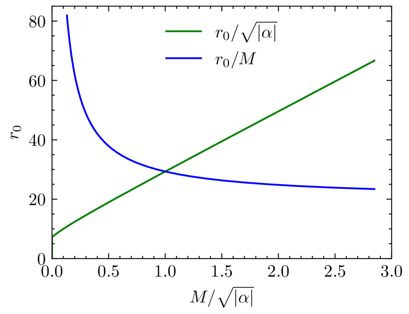
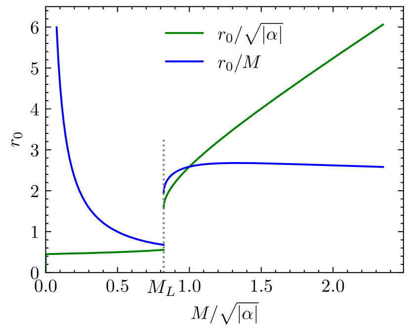
Figure 3: The plot shows the throat radius $r_{0}$ as a function of $M/\sqrt{|\alpha|}$, for $a=0.9$ (left plot, no discontinuity in $r_{0}$) and $a=0.1$ (right plot, discontinuity at $M_{L}$). The discontinuity corresponds to a change of branch in the solution of (34). In Fig. 2, different branches correspond to intersections of $A$ (black dashed curve) and $f$ (colored curves).

Obviously, the size of the throat increases with the parameter $a$. For example, it is easy to show that the throat radius quickly converges towards $r_{0}\approx 2M/\left(1-a\right)$ as soon as $M>\sqrt{\left\lvert\alpha\right\rvert}$ (which corresponds at most to the order of magnitude $M>10M_{\odot}$, according to the bounds on $\left\lvert\alpha\right\rvert$ given in the previous section). Hence a throat radius enhanced by a factor $\left(1-a\right)^{-1}$ with respect to the Schwarzschild radius for the corresponding mass.

We conclude our discussion by presenting the wormhole solutions using everywhere non-singular coordinates (including the throat). To do this we change the radial coordinate $r$ by introducing $l$ with range $l\in\left]-\infty,\infty\right[$ defined by

$$r^{2}=l^{2}+r_{0}^{2}$$ (41)

In this coordinate system, any wormhole metric, with throat $r_{0}$ of the form (37), is given by

$$\mathrm{d}s^{2}=-F\left(l\right)\mathrm{d}t^{2}+\frac{\mathrm{d}l^{2}}{H\left(l\right)}+\left(l^{2}+r_{0}^{2}\right)\mathrm{d}\Omega^{2},$$ (42)

where

$$F\left(l\right)=f\left(\sqrt{l^{2}+r_{0}^{2}}\right),\quad H\left(l\right)=h\left(\sqrt{l^{2}+r_{0}^{2}}\right)\frac{l^{2}+r_{0}^{2}}{l^{2}}.$$ (43)

Note that the function $H\left(l\right)$ is regular everywhere, and in particular at the throat $l\to 0$ we have,

$$H\left(l\right)=\frac{r_{0}}{2}h^{\prime}\left(r_{0}\right)+\mathcal{O}\left(l^{2}\right).$$ (44)

Since $h\left(r>r_{0}\right)>0$, hence $H\left(l\right)\geq 0$ everywhere. The other metric function, $F\left(l\right)$, is regular and non-negative everywhere. In Fig. 4, we plot the functions $F\left(l\right)$ and $H\left(l\right)$ for different masses $M$, when $a=0.1$. The masses of the yellow and red plots are chosen very close to the mass $M_{L}$ where occurs the $r_{0}$ discontinuity: for the yellow plot, the mass is still sufficiently low so that the throat $r_{0}$ is close to $r=0$ and blueshifted, while for the red plot, the throat $r_{0}$ is much larger and the spacetime is redshifted there. This is not just a sharp evolution of the $F\left(l\right)$ behavior as a function of the mass, but a true discontinuity at $M=M_{L}$.

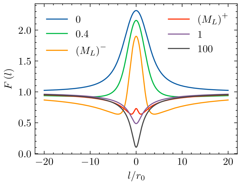
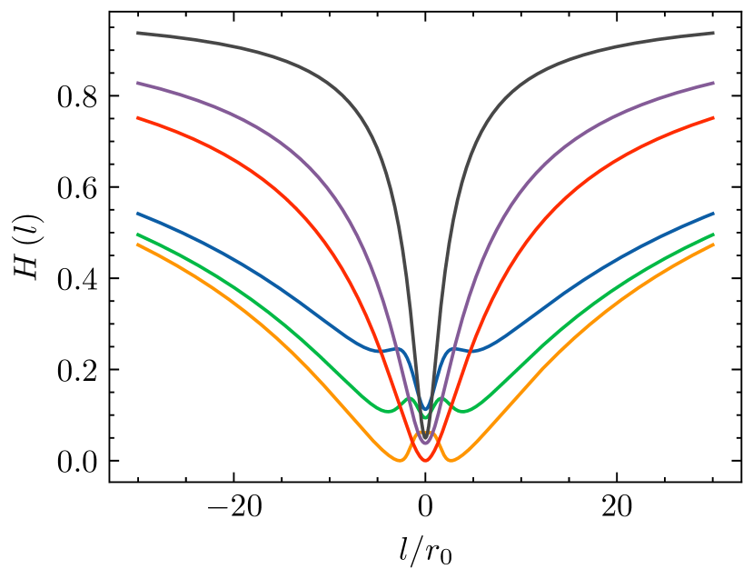
Figure 4: Functions $F\left(l\right)$ and $H\left(l\right)$ of metric (42) (with parameter $a=0.1$), for different values of $M/\sqrt{\left\lvert\alpha\right\rvert}$ given by the legend. The values $\left(M_{L}\right)^{-}$ and $\left(M_{L}\right)^{+}$ are as close as possible to the limit mass $M_{L}$ with our numerical precision, namely $\left(M_{L}\right)^{\pm}=M_{L}\left(1\pm 10^{-15}\right)$, illustrating the discontinuity occurring at this mass. For huge masses, the redshift function converges to the value $a$($=0.1$ here) at the throat.

IV Conclusions

In this paper we have studied solutions of the theory (2) as well as certain of its disformal versions. The theory (2) is in the class of Horndeski theory, and, thanks to underlying symmetries as well as a particular choice of relation between coupling constants, exact solutions can be found analytically.

We analyzed in detail the metric of a spherically symmetric solution (5-7), first found in Fernandes:2021dsb . Depending on the sign of the coupling $\alpha$ (and hence $\lambda$), the physical meaning of the solution may differ drastically. For positive $\alpha$ the spacetime (5) with (6) always describes a black hole with a singularity hidden by a horizon, similar to GR black holes. It is worth noting that for $\alpha>0$, either other spherically symmetric solutions describing spacetime outside a gravitating body exist, either $\alpha$ satisfies the tight constraint (11), implying virtually no modifications of GR for any present-day and near future observations. The case of $\alpha<0$ is more involved. Indeed, in this case there is a limiting mass $M_{\text{min}}$ given in terms of the parameters of the theory, Eq. (9). For $M>M_{\text{min}}$, the spacetime (5) with (6) describes a black hole. For $M\leq M_{\text{min}}$, the solution (5), (6) corresponds to a naked singularity.

The analysis of the black hole thermodynamics showed that the entropy of the black hole receives a $\log$-correction, Eq. (17), that depends only on the parameter $\alpha$ of the theory. Meanwhile, the first law of thermodynamics holds, with the Hawking temperature given by (18), that also depends on the coupling $\alpha$, while the mass is indeed given by $M$.

We then presented three new classes of solutions of (2). The first type is a non trivial flat solution, given by Eq. (21). The solution has a non-trivial scalar field, while the metric remains flat, i.e. the backreaction of the scalar field is absent in this case. The second solution is an extension of the black hole solution (5), (6) to a slowly rotating case, Eqs. (22), (23). Probably the most interesting case is the third new solution we found, an analogue of the Vaidya solution of GR. The solutions (24) and (25) describe correspondingly radiating and accreting solutions of the theory (2), that are counterparts of the Vaidya solution in GR. The mass of the black hole $M=M(v)$ ($M=M(u)$) grows (decreases) due to the infall (radiation) of light dust.

The last part of the paper is devoted to the disformal transformations of theory (2) and its solutions. We focused on the case $\alpha<0$ where the theory admits naked singularities for small enough masses $M<M_{\text{min}}$. We proposed a remedy to avoid the pathology by coupling matter to a disformed metric, which amounts to making a disformal transformation of the theory (26). We first showed that a very simple choice of disformal parameter $D=D(X)$ led to a theory admitting gravitating monopole-like solutions, and where the $M=0$ spacetime is regular at $r=0$. On the other hand, we found a general form of the disformal parameter $D=D(\phi,X)$, such that the naked singularity of the original theory is transformed to a wormhole whose metric is regular everywhere, for any mass $M$. An interesting feature of the obtained solutions is that wormholes with both redshift and blueshift at the throat exist. The blueshift at the throat implies that the light traveling through a wormhole experiences blueshift as it approaches the throat, which is in contrast to the standard behaviour, e.g. in the case of GR, when light is always redshifted near gravitating sources.

Several questions arise on other choices of disforming functions $D(\phi,X)$, as well as the analysis of stability for the obtained wormhole solutions. It has been shown before that there are no stable wormholes in Horndeski theory Evseev:2017jek , while the extensions of Horndeski theory have a chance to support stable wormholes Mironov:2018uou ; Franciolini:2018aad . Therefore it remains to be seen whether our wormhole solutions in beyond Horndeski theory are stable or not. It would be also important to explore in detail observational features of the wormholes, such as light rings, shadows, and contrast them with compact objects of GR. It would also be interesting to look for stationary metrics within this theory (2). The presence of an always valid geometric constraint may give a hint on the form of stationary solutions. Last but not least it would be interesting to study neighbouring theories to (2) and find spherically symmetric solutions there. These are some of the intriguing questions we hope will be studied in the near future.

Appendix A Theories and solutions arising from the initial action

A.1 Known solutions

We evoked in the introduction the existence of other relevant theories arising from the original action (2), with $\lambda=3\beta^{2}/\left(4\alpha\right)$ or $\beta=0=\lambda$. It was shown in Fernandes:2021dsb (see also Charmousis:2021npl ) that they admit the following asymptotically flat, spherically symmetric solution:

$$\mathrm{d}s^{2}=-f(r)\mathrm{d}t^{2}+\frac{\mathrm{d}r^{2}}{f(r)}+r^{2}\mathrm{d}\Omega^{2},\quad f(r)=1+\frac{r^{2}}{2\alpha}\left(1-\sqrt{1+\frac{8\alpha M}{r^{3}}}\right),$$ (45)

for any ADM mass $M$, along with the respective scalar field profiles:

$$\phi=\ln\left(\frac{\sqrt{-2\alpha/\beta}}{r}\right)-\ln\cosh\left(c_{3}\pm\int\frac{\mathrm{d}r}{r\sqrt{f}}\right),\quad\phi=\int\mathrm{d}r\frac{\pm 1-\sqrt{f}}{r\sqrt{f}}.$$ (46)

The scalar field constant $c_{3}$ is unconstrained, while the second profile is defined up to an additive constant, since (2) with $\beta=0=\lambda$ is the shift-symmetric four dimensional Einstein-Gauss-Bonnet (EGB) theory, see Fernandes:2020nbq . We can thus, for this latter theory, add a linear time dependence for the scalar field: $\phi=\mu t+\psi(r)$, with $\mu$ a constant, without breaking the spherical symmetry of the scalar field derivatives. This was done in Charmousis:2021npl and leads to

$$\psi=\int\mathrm{d}r\frac{\pm\sqrt{\mu^{2}r^{2}+f}-f}{rf},$$ (47)

and one finds that for any $\mu$, this profile is solution, along with an unchanged spacetime (45). For $\mu=0$, the linear time dependence disappears, and one recovers the previous profile of (46).
We will now, in a similar fashion to the body of the paper, focus on flat spacetime, slowly rotating and radiating solutions for the above two theories.

A.2 Flat spacetime solutions

As opposed to what we studied in the main text, the obtained spacetime (45) does reduce to flat spacetime as $M\to 0$, that is to say $f(r)\to 1$. In this case, the scalar fields of (46) reduce to:

$$\phi=\ln\left(\frac{\mu\sqrt{-8\alpha/\beta}}{1+\mu^{2}r^{2}}\right)$$ (48)

where $\mu=\exp\left(\pm c_{3}\right)$ for the first one, and:

$$\phi=0\quad\text{or}\quad\phi=-2\ln r$$ (49)

up to an additive constant for the second one, for the respective choice of plus or minus sign. As regards the solution (47) with $\phi=\mu t+\psi(r)$, it corresponds to the same spacetime and therefore gives another possibility for a stealth flat spacetime solution as $M\to 0$, with a scalar field reducing to:

$$\phi=\mu t-\ln r\pm\left(\sqrt{\mu^{2}r^{2}+1}-\operatorname{arctanh}\sqrt{\mu^{2}r^{2}+1}\right).$$ (50)

We can nevertheless question if other flat spacetime solutions, with $\phi=\phi\left(t,r\right)$, exist. We find the following solutions: on the one hand, when $\lambda=3\beta^{2}/\left(4\alpha\right)$,

$$\phi={} \phi(r)=\ln\left(\frac{\mu\sqrt{-8\alpha/\beta}}{1+\mu^{2}r^{2}}\right),$$ (51)

$$\phi={} \phi(t)=\ln\left(\frac{\sqrt{-2\alpha/\beta}}{\left\lvert t+\mu\right\rvert}\right),$$ (52)

$$\phi={} \phi(t,r)=\ln\left(\frac{\sqrt{-8\mu\alpha/\beta}}{\left\lvert r^{2}-t^{2}+\mu\right\rvert}\right).$$ (53)

The first line, as shown above, comes directly from the black hole scalar field as $M\to 0$, while the other lines are different branches. In each case, $\mu$ is an integration constant. Only the first branch is differentiable in the whole spacetime. On the other hand, when $\beta=0=\lambda$, one gets up to a constant,

$$\phi={} 0,$$ (54)

$$\phi={} \phi(r)=-2\ln r,$$ (55)

$$\phi={} \phi(t,r)=\mu t-\ln r\pm\left(\sqrt{\mu^{2}r^{2}+1}-\operatorname{arctanh}\sqrt{\mu^{2}r^{2}+1}\right),$$ (56)

$$\phi={} \phi(t,r)=-\ln\left\lvert r^{2}-t^{2}\right\rvert.$$ (57)

The only new solution not described above is the last one. The constant profile and the $+$ branch of (56) are differentiable for any $r\geq 0$.

A.3 Slowly rotating solutions

Let’s now turn to the slowly rotating solutions. The ansatz metric is the same (22) as in the main text, and the same discussion is still valid: one gets the same $f(r)$ (45) and scalar fields (46) (or also the time-dependent scalar field $\phi=\mu t+\psi\left(r\right)$, (47)) as in spherical symmetry. Finally, $\omega\left(r\right)$ is given by

$$\omega(r)=-6aM\int_{\infty}^{r}\frac{\mathrm{d}r}{r^{4}\sqrt{1+\frac{8\alpha M}{r^{3}}}}=-\frac{a}{2\alpha}\left(1-\sqrt{1+\frac{8\alpha M}{r^{3}}}\right),$$ (58)

where, once again, the GR limit is fulfilled asymptotically. The slowly rotating metric is therefore the same for both theories, with different scalar fields. Note that, for $\beta=0=\lambda$, the slowly rotating solution has already been given in Charmousis:2021npl .

A.4 Radiating solutions

We proceed with the Vaidya-like solutions. While we ended up with an unchanged spherically-symmetric scalar field in the body of the paper, this is no longer the case: the dependence of the scalar field on the null coordinate $u$ or $v$ is no longer trivial. In fact, one finds that the scalar field must satisfy a non-linear partial differential equation (PDE) which does not admit any obvious solution. But, assuming this PDE is satisfied, i.e. taking it as an implicit definition for the scalar field, all field equations are satisfied, and one ends up with the following outgoing-Vaidya-like solution

$$\left\{\begin{split}&\mathrm{d}s^{2}=-f\left(u,r\right)\mathrm{d}u^{2}-2\mathrm{d}u\mathrm{d}r+r^{2}\mathrm{d}\Omega^{2},\quad f\left(u,r\right)=1+\frac{r^{2}}{2\alpha}\left(1-\sqrt{1+\frac{8\alpha M(u)}{r^{3}}}\right),\\ &0=2\alpha\left(f\left(r\phi^{\prime}+1\right)^{2}-2r\dot{\phi}\left(r\phi^{\prime}+1\right)-1\right)-\beta r^{2}e^{2\phi},\quad T_{uu}=-\frac{M^{\prime}(u)}{4\pi r^{2}}\geq 0,\end{split}\right.$$ (59)

and the following ingoing-Vaidya-like solution

$$\left\{\begin{split}&\mathrm{d}s^{2}=-f\left(v,r\right)\mathrm{d}v^{2}+2\mathrm{d}v\mathrm{d}r+r^{2}\mathrm{d}\Omega^{2},\quad f\left(v,r\right)=1+\frac{r^{2}}{2\alpha}\left(1-\sqrt{1+\frac{8\alpha M(v)}{r^{3}}}\right),\\ &0=2\alpha\left(f\left(r\phi^{\prime}+1\right)^{2}+2r\dot{\phi}\left(r\phi^{\prime}+1\right)-1\right)-\beta r^{2}e^{2\phi},\quad T_{vv}=\frac{M^{\prime}(v)}{4\pi r^{2}}\geq 0.\end{split}\right.$$ (60)

The PDE taken as an implicit definition of the scalar field is given below the metric, and with, of course, $\beta=0$ for the shift-symmetric four dimensional EGB case. A prime denotes derivation with respect to $r$, while a dot stands for derivation with respect to $u$ or $v$.

Appendix B Disformal transformations

The gravitating monopole-like solution solves the following beyond Horndeski theory, where for readability, the variables $\phi$ and $\tilde{X}$ (the disformed kinetic term) are replaced respectively by $y$ and $x$,

$$\tilde{G_{2}}\left(y,x\right)={} 8\sqrt{5\sqrt{2}+7}\alpha x^{2}+12\sqrt{\sqrt{2}+1}\beta x\mathrm{e}^{2y}-\frac{\sqrt{\sqrt{2}-1}\beta^{2}\mathrm{e}^{4y}}{2\alpha}+8\sqrt{2\left(\sqrt{2}-1\right)}\beta x\mathrm{e}^{2y}\ln\left\lvert x\right\rvert,$$

$$\tilde{G_{3}}\left(y,x\right)={} 8\left(\sqrt{2}+1\right)^{3/2}\alpha x+4\sqrt{2\left(\sqrt{2}-1\right)}\beta\mathrm{e}^{2y}+2\sqrt{2\left(\sqrt{2}-1\right)}\beta\mathrm{e}^{2y}\ln\left\lvert x\right\rvert,$$

$$\tilde{G_{4}}\left(y,x\right)={} \sqrt{\sqrt{2}-1}+4\sqrt{\sqrt{2}+1}\alpha x-\sqrt{\sqrt{2}-1}\beta\mathrm{e}^{2y},$$

$$\tilde{G_{5}}\left(y,x\right)={} \frac{4\alpha\ln\left\lvert x\right\rvert}{\sqrt{\sqrt{2}-1}},$$

$$\tilde{F_{4}}\left(y,x\right)={} \frac{\sqrt{\sqrt{2}-1}(\beta\mathrm{e}^{2y}-1)}{2\sqrt{2}x^{2}}+\frac{\sqrt{2\left(\sqrt{2}+1\right)}\alpha}{x},$$

$$\tilde{F_{5}}\left(y,x\right)={} \frac{\left(\sqrt{2}-2\right)\alpha}{3\left(\sqrt{2}-1\right)^{3/2}x^{2}}.$$

The main differences (apart from the beyond Horndeski terms) with the original theory (3) are the terms proportional to $\ln|x|$ in $\tilde{G_{2}}$ and $\tilde{G_{3}}$.

More generally, we now present the disformed Horndeski action which arises through a disformal transformation (26) of a general starting Horndeski action (1-I). The disformed Horndeski action belongs to the so-called beyond Horndeski theory and is given by

$$S=\int\mathrm{d}^{4}x\sqrt{-\tilde{g}}\left\{\mathcal{\tilde{L}}_{2}+\mathcal{\tilde{L}}_{3}+\mathcal{\tilde{L}}_{4}+\mathcal{\tilde{L}}_{5}+\mathcal{\tilde{L}}_{4b}+\mathcal{\tilde{L}}_{5b}\right\},$$ (61)

where appear the two additional beyond Horndeski Lagrangians that read

$$\mathcal{\tilde{L}}_{4b}=\tilde{F_{4}}\left(\phi,\tilde{X}\right)\left\{2\tilde{X}\left[\left(\tilde{\Box\phi}\right)^{2}-\left(\tilde{\phi}_{\mu\nu}\right)^{2}\right]+2\left[\tilde{\Box\phi}\tilde{\phi}^{\mu}\tilde{\phi}_{\mu\nu}\tilde{\phi}^{\nu}-\tilde{\phi}_{\mu}\tilde{\phi}^{\mu\nu}\tilde{\phi}_{\nu\rho}\tilde{\phi}^{\rho}\right]\right\},$$

$$\mathcal{\tilde{L}}_{5b}=\tilde{F_{5}}\left(\phi,\tilde{X}\right)\left\{2\tilde{X}\left[\left(\tilde{\Box\phi}\right)^{3}-3\tilde{\Box\phi}\left(\tilde{\phi}_{\mu\nu}\right)^{2}+2\tilde{\phi}_{\mu\nu}\tilde{\phi}^{\nu\rho}\tilde{\phi}{{}^{\mu}_{\rho}}\right]\right.$$

$$\left.\qquad+3\left[\left(\tilde{\Box\phi}\right)^{2}\tilde{\phi}^{\mu}\tilde{\phi}_{\mu\nu}\tilde{\phi}^{\nu}-2\tilde{\Box\phi}\tilde{\phi}_{\mu}\tilde{\phi}^{\mu\nu}\tilde{\phi}_{\nu\rho}\tilde{\phi}^{\rho}-\tilde{\phi}_{\mu\nu}\tilde{\phi}^{\mu\nu}\tilde{\phi}^{\rho}\tilde{\phi}_{\rho\sigma}\tilde{\phi}^{\sigma}+2\tilde{\phi}_{\mu}\tilde{\phi}^{\mu\rho}\tilde{\phi}_{\rho\nu}\tilde{\phi}^{\nu\sigma}\tilde{\phi}_{\sigma}\right]\right\},$$

where $\tilde{\phi}_{\mu}=\tilde{\nabla}_{\mu}\phi$ and $\tilde{X}=\frac{X}{1-2DX}$. The disformed Horndeski functions $\tilde{G_{k}}\left(\phi,\tilde{X}\right)$ are given by

$$\tilde{G_{2}}={} G_{2}\sqrt{1+2D\tilde{X}}-2\tilde{X}\left(H_{3}+H_{4}+H_{5}\right)_{\phi}-\frac{2\tilde{X}^{2}G_{3}D_{\phi}}{\left(1+2D\tilde{X}\right)^{3/2}},$$

$$\tilde{G_{3}}={} \frac{G_{3}}{\sqrt{1+2D\tilde{X}}}-\left(H_{3}+H_{4}+H_{5}\right)$$

$$\quad+2\tilde{X}\left\{H_{R,\phi\phi}-H_{\Box,\phi}+\frac{1}{\sqrt{1+2D\tilde{X}}}\left[2DG_{4\phi}-D_{\phi}\left(\frac{2\tilde{X}G_{4\tilde{X}}}{1-2\tilde{X}^{2}D_{\tilde{X}}}-G_{4}\right)\right]\right\},$$

$$\tilde{G_{4}}={} G_{4}\sqrt{1+2D\tilde{X}}+\tilde{X}\left(H_{R,\phi}-\frac{\tilde{X}G_{5}D_{\phi}}{\left(1+2D\tilde{X}\right)^{3/2}}\right),$$

$$\tilde{G_{5}}={} \frac{G_{5}}{\sqrt{1+2D\tilde{X}}}+H_{R},$$

while the beyond Horndeski functions $\tilde{F_{k}}\left(\phi,\tilde{X}\right)$ read

$$\tilde{F_{4}}={} \frac{D_{\tilde{X}}}{2}\left(\frac{2\tilde{X}G_{4\tilde{X}}\sqrt{1+2D\tilde{X}}}{1-2\tilde{X}^{2}D_{\tilde{X}}}-\frac{G_{4}}{\sqrt{1+2D\tilde{X}}}\right)-\frac{1}{2}H_{R,\phi\tilde{X}}-\frac{\tilde{X}^{3}G_{5\tilde{X}}D_{\tilde{X}}D_{\phi}}{\left(1-2\tilde{X}^{2}D_{\tilde{X}}\right)\left(1+2D\tilde{X}\right)^{3/2}},$$

$$\quad+\frac{G_{5\phi}D}{2\left(1+2D\tilde{X}\right)^{3/2}}+\frac{G_{5}}{2\left(1+2D\tilde{X}\right)^{5/2}}\left\{\tilde{X}\left(1+2D\tilde{X}\right)D_{\phi\tilde{X}}+D_{\phi}\left[1-\tilde{X}\left(D+3\tilde{X}D_{\tilde{X}}\right)\right]\right\}$$

$$\tilde{F_{5}}={} -\frac{\tilde{X}G_{5\tilde{X}}D_{\tilde{X}}}{6\left(1-2\tilde{X}^{2}D_{\tilde{X}}\right)\sqrt{1+2D\tilde{X}}}.$$

For clarity, we have defined the following functions

$$H_{\Box}=\frac{\tilde{X}G_{5}D_{\phi}}{\left(1+2D\tilde{X}\right)^{3/2}},\quad H_{R}=\int\mathrm{d}\tilde{X}\frac{G_{5}\left(D+\tilde{X}D_{\tilde{X}}\right)}{\left(1+2D\tilde{X}\right)^{3/2}},\quad H_{5}=\int\mathrm{d}\tilde{X}\left(H_{\Box,\phi}-H_{R,\phi\phi}\right),$$

and

$$H_{3}=\int\mathrm{d}\tilde{X}\frac{-G_{3}\left(D+\tilde{X}D_{\tilde{X}}\right)}{\left(1+2D\tilde{X}\right)^{3/2}},\quad H_{4}=\int\frac{\mathrm{d}\tilde{X}}{\sqrt{1+2D\tilde{X}}}\left[D_{\phi}\left(\frac{2\tilde{X}G_{4\tilde{X}}}{1-2\tilde{X}^{2}D_{\tilde{X}}}-G_{4}\right)-2DG_{4\phi}\right],$$

thus following the notations of Bettoni:2013diz , with the difference that we are including an $X$ dependence for the disformal function.

Let us now apply this disformal transformation to our specific action (2) and its solution (5-7) with the following choice of $W^{-1}$,

$$W^{-1}\left(\phi,X\right)\equiv\left(1-2D\left(\phi,X\right)X\right)^{-1}=\left(1-1/a\right)^{-1}\left(1+2B\left(\phi\right)X\right),\quad 0<a<1,$$ (62)

see eq. (33) with

$$B(\phi)=\frac{\psi^{2}}{A\left(\psi/\sqrt{\left\lvert\alpha\right\rvert}\right)},\quad\psi=\sqrt{\frac{-2\alpha}{\beta}}\mathrm{e}^{-\phi}.$$

Since $\tilde{X}$ is a second-order polynomial in $X$, one gets two possible solutions for $X$ given by

$$X=\frac{-1}{4B\left(\phi\right)}\left(1\pm S\left(\phi,\tilde{X}\right)\right),\quad S\left(\phi,\tilde{X}\right)\equiv\sqrt{1+8B\left(\phi\right)\left(1-\frac{1}{a}\right)\tilde{X}}$$ (63)

Depending on which sign is chosen ($+$ or $-$), one is led to two distinct disformed actions, $S_{+}$ and $S_{-}$ respectively. One must therefore identify which variational principle is solved by the disformed metric (37-39). To this aim, one has to analyze the situation on-shell where

$$S\left(\phi,\tilde{X}\right)=\left\lvert s\left(r\right)\right\rvert,\quad s\left(r\right)\equiv 1-2B\left(\phi\right)\frac{f\left(r\right)}{r^{2}},\quad\phi=\ln\left(\frac{\sqrt{-2\alpha/\beta}}{r}\right).$$ (64)

This in turn implies that

$$\frac{-f\left(r\right)}{2r^{2}}=\frac{-1}{4B\left(\phi\right)}\left(1\pm\left\lvert s\left(r\right)\right\rvert\right)$$ (65)

and, this is consistent only by choosing the $+$ sign when $s\left(r\right)\leq 0$, and the $-$ sign when $s\left(r\right)\geq 0$. As a consequence, the disformed metric solves the equations of motion of $S_{+}$ (resp. of $S_{-}$) if and only if $s\left(r\right)\leq 0$ (resp. if $s\left(r\right)\geq 0$). In particular, it will be problematic to define an action principle for the disformed theory if the function $s\left(r\right)$ has a nonconstant sign. Note that $s\left(r\right)$ changes sign precisely at the singular radius $r_{*}$ identified in (35), thus, we retrieve the necessity of hiding $r_{*}$ below the wormhole throat. This is for instance ensured by our choice (36), for which $s\left(r\right)<0$ in the whole physical spacetime, and hence a well-defined action principle is shown to exist. The corresponding beyond Horndeski theory is given by (for readability, we write coefficients as functions of variables $\left(y,x\right)$, where $y$ stands for $\phi$ and $x$ for $\tilde{X}$):

$$\tilde{F_{5}}\left(y,x\right)={} \frac{2(a-1)\alpha\sqrt{-\frac{xB(y)}{S\left(y,x\right)+1}}\left(aS\left(y,x\right)+4(a-1)xB(y)-2S\left(y,x\right)+a\right)}{3ax^{2}S\left(y,x\right)\left(a\left(S\left(y,x\right)-1\right)-4(a-1)xB(y)\right)},$$

$$\tilde{G_{5}}\left(y,x\right)={} \frac{2\alpha\ln\left(\frac{S\left(y,x\right)+1}{4B(y)}\right)}{\sqrt{-\frac{xB(y)}{S\left(y,x\right)+1}}}+\frac{8\alpha\sqrt{S\left(y,x\right)-1}\arctan\left(\frac{\sqrt{S\left(y,x\right)-1}}{\sqrt{2}}\right)-4\sqrt{2}\alpha\ln\left(\frac{S\left(y,x\right)+1}{4B(y)}\right)}{\sqrt{\frac{a-aS\left(y,x\right)}{a-1}}},$$

$$\tilde{G_{4}}\left(y,x\right)={} \frac{1}{B(y)\sqrt{-\frac{xB(y)}{S\left(y,x\right)+1}}\sqrt{\frac{a-aS\left(y,x\right)}{a-1}}\left(a\left(-S\left(y,x\right)\right)+8(a-1)xB(y)+a\right)}\left\{4\alpha xB^{\prime}(y)\left((a-1)xB(y)\right.\right.$$

$$\left.\left.\left(8\sqrt{2}\sqrt{-\frac{xB(y)}{S\left(y,x\right)+1}}-\left(\sqrt{\frac{a-aS\left(y,x\right)}{a-1}}-2\sqrt{2}\sqrt{-\frac{xB(y)}{S\left(y,x\right)+1}}\right)\ln\left(\frac{S\left(y,x\right)+1}{4B(y)}\right)\right)-\right.\right.$$

$$\left.\left.\sqrt{2}a\left(S\left(y,x\right)-1\right)\sqrt{-\frac{xB(y)}{S\left(y,x\right)+1}}\right)\right\}+2\sqrt{-\frac{xB(y)}{S\left(y,x\right)+1}}\left(-\frac{\alpha\left(S\left(y,x\right)+1\right)}{B(y)}-\beta\mathrm{e}^{2y}+1\right),$$

and where the expressions for $\tilde{G_{2}}$, $\tilde{G_{3}}$ and $\tilde{F_{4}}$ are too cumbersome to report.

References

- (1) M. S. Morris and K. S. Thorne, Am. J. Phys. 56 (1988), 395-412 doi:10.1119/1.15620
- (2) B. P. Abbott et al. [LIGO Scientific and Virgo], Phys. Rev. Lett. 119, no.16, 161101 (2017) doi:10.1103/PhysRevLett.119.161101 [arXiv:1710.05832 [gr-qc]].
- (3) R. Abbott et al. [LIGO Scientific and Virgo], Astrophys. J. Lett. 896, no.2, L44 (2020) doi:10.3847/2041-8213/ab960f [arXiv:2006.12611 [astro-ph.HE]].
- (4) R. Abbott et al. [LIGO Scientific, KAGRA and VIRGO], Astrophys. J. Lett. 915, no.1, L5 (2021) doi:10.3847/2041-8213/ac082e [arXiv:2106.15163 [astro-ph.HE]].
- (5) C. Charmousis, A. Lehébel, E. Smyrniotis and N. Stergioulas, JCAP 02, no.02, 033 (2022) doi:10.1088/1475-7516/2022/02/033 [arXiv:2109.01149 [gr-qc]].
- (6) G. W. Horndeski, Int. J. Theor. Phys. 10, 363-384 (1974) doi:10.1007/BF01807638
- (7) E. Babichev and C. Charmousis, JHEP 08, 106 (2014) doi:10.1007/JHEP08(2014)106 [arXiv:1312.3204 [gr-qc]]. T. Kobayashi and N. Tanahashi, PTEP 2014, 073E02 (2014) doi:10.1093/ptep/ptu096 [arXiv:1403.4364 [gr-qc]]. C. Charmousis and D. Iosifidis, J. Phys. Conf. Ser. 600 (2015), 012003 doi:10.1088/1742-6596/600/1/012003 [arXiv:1501.05167 [gr-qc]]. M. Minamitsuji and J. Edholm, Phys. Rev. D 100, no.4, 044053 (2019) doi:10.1103/PhysRevD.100.044053 [arXiv:1907.02072 [gr-qc]].
- (8) J. Ben Achour, H. Liu and S. Mukohyama, JCAP 02, 023 (2020) doi:10.1088/1475-7516/2020/02/023 [arXiv:1910.11017 [gr-qc]]. K. Takahashi and H. Motohashi, JCAP 06 (2020), 034 doi:10.1088/1475-7516/2020/06/034 [arXiv:2004.03883 [gr-qc]].
- (9) E. Babichev, C. Charmousis and A. Lehébel, JCAP 1704 (2017) 027, doi: 10.1088/1475-7516/2017/04/027; E. Babichev and A. Lehébel, JCAP 12 (2018), 027, doi: 10.1088/1475-7516/2018/12/027; J. Chagoya and G. Tasinato, JCAP 1808, 006 (2018), doi: 10.1088/1475-7516/2018/08/006; T. Kobayashi and T. Hiramatsu, Phys. Rev. D 97 (2018) no.10, 104012, doi: 10.1103/PhysRevD.97.104012; A. Lehébel, E. Babichev and C. Charmousis, JCAP 07 (2017), 037 doi:10.1088/1475-7516/2017/07/037 [arXiv:1706.04989 [gr-qc]]. M. Minamitsuji and J. Edholm, Phys. Rev. D 101, no. 4, 044034 (2020), doi: 10.1103/PhysRevD.101.044034 A. Bakopoulos, C. Charmousis, P. Kanti and N. Lecoeur, [arXiv:2203.14595 [gr-qc]].
- (10) N. M. Bocharova, K. A. Bronnikov and V. N. Melnikov, Vestn.Mosk.Univ.Ser.III Fiz.Astron. (1970) 6, 706-709
- (11) J. D. Bekenstein, Annals Phys. 82, 535-547 (1974) doi:10.1016/0003-4916(74)90124-9
- (12) C. Klimcik, J. Math. Phys. 34, 1914-1926 (1993) doi:10.1063/1.530146
- (13) C. Martinez, R. Troncoso and J. Zanelli, Phys. Rev. D 67, 024008 (2003) doi:10.1103/PhysRevD.67.024008 [arXiv:hep-th/0205319 [hep-th]].
- (14) C. Martinez, J. P. Staforelli and R. Troncoso, Phys. Rev. D 74, 044028 (2006) doi:10.1103/PhysRevD.74.044028 [arXiv:hep-th/0512022 [hep-th]].
- (15) P. G. S. Fernandes, Phys. Rev. D 103, no.10, 104065 (2021) doi:10.1103/PhysRevD.103.104065 [arXiv:2105.04687 [gr-qc]].
- (16) C. Charmousis, B. Gouteraux and E. Kiritsis, JHEP 09 (2012), 011 doi:10.1007/JHEP09(2012)011 [arXiv:1206.1499 [hep-th]].
- (17) G. Dotti and R. J. Gleiser, Phys. Lett. B 627 (2005), 174-179 doi:10.1016/j.physletb.2005.08.110 [arXiv:hep-th/0508118 [hep-th]].
- (18) C. Bogdanos, C. Charmousis, B. Gouteraux and R. Zegers, JHEP 10 (2009), 037 doi:10.1088/1126-6708/2009/10/037 [arXiv:0906.4953 [hep-th]].
- (19) D. Glavan and C. Lin, Phys. Rev. Lett. 124 (2020) no.8, 081301 doi:10.1103/PhysRevLett.124.081301 [arXiv:1905.03601 [gr-qc]].
- (20) M. Zumalacárregui and J. García-Bellido, Phys. Rev. D 89 (2014), 064046 doi:10.1103/PhysRevD.89.064046 [arXiv:1308.4685 [gr-qc]].
- (21) J. Ben Achour, D. Langlois and K. Noui, Phys. Rev. D 93, no.12, 124005 (2016) doi:10.1103/PhysRevD.93.124005 [arXiv:1602.08398 [gr-qc]].
- (22) T. Anson, E. Babichev, C. Charmousis and M. Hassaine, JHEP 01, 018 (2021) doi:10.1007/JHEP01(2021)018 [arXiv:2006.06461 [gr-qc]].
- (23) C. Charmousis, M. Crisostomi, R. Gregory and N. Stergioulas, Phys. Rev. D 100 (2019) no.8, 084020 doi:10.1103/PhysRevD.100.084020 [arXiv:1903.05519 [hep-th]].
- (24) T. Anson, E. Babichev and C. Charmousis, Phys. Rev. D 103 (2021) no.12, 124035 doi:10.1103/PhysRevD.103.124035 [arXiv:2103.05490 [gr-qc]].
- (25) A. Bakopoulos, C. Charmousis and P. Kanti, JCAP 05 (2022) no.05, 022 doi:10.1088/1475-7516/2022/05/022 [arXiv:2111.09857 [gr-qc]].
- (26) V. Faraoni and A. Leblanc, JCAP 08 (2021), 037 doi:10.1088/1475-7516/2021/08/037 [arXiv:2107.03456 [gr-qc]].
- (27) N. Chatzifotis, E. Papantonopoulos and C. Vlachos, Phys. Rev. D 105 (2022) no.6, 064025 doi:10.1103/PhysRevD.105.064025 [arXiv:2111.08773 [gr-qc]].
- (28) P. Kanti, B. Kleihaus and J. Kunz, Phys. Rev. Lett. 107 (2011), 271101 doi:10.1103/PhysRevLett.107.271101 [arXiv:1108.3003 [gr-qc]]. P. Kanti, B. Kleihaus and J. Kunz, Phys. Rev. D 85 (2012), 044007 doi:10.1103/PhysRevD.85.044007 [arXiv:1111.4049 [hep-th]]. G. Antoniou, A. Bakopoulos, P. Kanti, B. Kleihaus and J. Kunz, Phys. Rev. D 101 (2020) no.2, 024033 doi:10.1103/PhysRevD.101.024033 [arXiv:1904.13091 [hep-th]].
- (29) D. Lovelock, J. Math. Phys. 12 (1971), 498-501 doi:10.1063/1.1665613
- (30) C. Charmousis, Lect. Notes Phys. 769 (2009), 299-346 doi:10.1007/978-3-540-88460-6_8 [arXiv:0805.0568 [gr-qc]].
- (31) H. Lu and Y. Pang, Phys. Lett. B 809 (2020), 135717 doi:10.1016/j.physletb.2020.135717 [arXiv:2003.11552 [gr-qc]]. R. A. Hennigar, D. Kubizňák, R. B. Mann and C. Pollack, JHEP 07 (2020), 027 doi:10.1007/JHEP07(2020)027 [arXiv:2004.09472 [gr-qc]].
- (32) P. G. S. Fernandes, P. Carrilho, T. Clifton and D. J. Mulryne, Class. Quant. Grav. 39 (2022) no.6, 063001 doi:10.1088/1361-6382/ac500a [arXiv:2202.13908 [gr-qc]].
- (33) L. Hui and A. Nicolis, Phys. Rev. Lett. 110 (2013), 241104 doi:10.1103/PhysRevLett.110.241104 [arXiv:1202.1296 [hep-th]]. T. P. Sotiriou and S. Y. Zhou, Phys. Rev. D 90 (2014), 124063 doi:10.1103/PhysRevD.90.124063 [arXiv:1408.1698 [gr-qc]]. E. Babichev, C. Charmousis and A. Lehébel, Class. Quant. Grav. 33 (2016) no.15, 154002 doi:10.1088/0264-9381/33/15/154002 [arXiv:1604.06402 [gr-qc]].
- (34) R. C. Myers and J. Z. Simon, Phys. Rev. D 38 (1988), 2434-2444 doi:10.1103/PhysRevD.38.2434
- (35) T. Clunan, S. F. Ross and D. J. Smith, Class. Quant. Grav. 21 (2004), 3447-3458 doi:10.1088/0264-9381/21/14/009 [arXiv:gr-qc/0402044 [gr-qc]].
- (36) V. Iyer and R. M. Wald, Phys. Rev. D 50, 846-864 (1994) doi:10.1103/PhysRevD.50.846 [arXiv:gr-qc/9403028 [gr-qc]].
- (37) E. Ayon-Beato, C. Martinez, R. Troncoso and J. Zanelli, Phys. Rev. D 71 (2005), 104037 doi:10.1103/PhysRevD.71.104037 [arXiv:hep-th/0505086 [hep-th]].
- (38) E. Ayon-Beato, C. Martinez and J. Zanelli, Gen. Rel. Grav. 38, 145-152 (2006) doi:10.1007/s10714-005-0213-x [arXiv:hep-th/0403228 [hep-th]].
- (39) C. Charmousis, Lect. Notes Phys. 892, 25-56 (2015) doi:10.1007/978-3-319-10070-8_2 [arXiv:1405.1612 [gr-qc]]. C. Charmousis and D. Iosifidis, J. Phys. Conf. Ser. 600 (2015), 012003 doi:10.1088/1742-6596/600/1/012003 [arXiv:1501.05167 [gr-qc]].
- (40) J. B. Hartle, Astrophys. J. 150 (1967), 1005-1029 doi:10.1086/149400
- (41) J. B. Hartle and K. S. Thorne, Astrophys. J. 153 (1968), 807 doi:10.1086/149707
- (42) A. Bakopoulos, C. Charmousis, P. Kanti and N. Lecoeur, [arXiv:2203.14595 [gr-qc]].
- (43) D. Bettoni and S. Liberati, Phys. Rev. D 88 (2013), 084020 doi:10.1103/PhysRevD.88.084020 [arXiv:1306.6724 [gr-qc]].
- (44) J. Gleyzes, D. Langlois, F. Piazza and F. Vernizzi, JCAP 02 (2015), 018 doi:10.1088/1475-7516/2015/02/018 [arXiv:1408.1952 [astro-ph.CO]].
- (45) M. Barriola and A. Vilenkin, Phys. Rev. Lett. 63 (1989), 341 doi:10.1103/PhysRevLett.63.341
- (46) T. Damour and S. N. Solodukhin, Phys. Rev. D 76 (2007), 024016 doi:10.1103/PhysRevD.76.024016 [arXiv:0704.2667 [gr-qc]]. Bettoni:2013diz
- (47) D. Bettoni and S. Liberati, Phys. Rev. D 88 (2013), 084020 doi:10.1103/PhysRevD.88.084020 [arXiv:1306.6724 [gr-qc]].
- (48) O. A. Evseev and O. I. Melichev, Phys. Rev. D 97 (2018) no.12, 124040 doi:10.1103/PhysRevD.97.124040 [arXiv:1711.04152 [gr-qc]].
- (49) S. Mironov, V. Rubakov and V. Volkova, Class. Quant. Grav. 36 (2019) no.13, 135008 doi:10.1088/1361-6382/ab2574 [arXiv:1812.07022 [hep-th]].
- (50) G. Franciolini, L. Hui, R. Penco, L. Santoni and E. Trincherini, JHEP 01 (2019), 221 doi:10.1007/JHEP01(2019)221 [arXiv:1811.05481 [hep-th]].
- (51) P. G. S. Fernandes, P. Carrilho, T. Clifton and D. J. Mulryne, Phys. Rev. D 102 (2020) no.2, 024025 doi:10.1103/PhysRevD.102.024025 [arXiv:2004.08362 [gr-qc]].