Optical Spin Initialisation and Readout with a Cavity-Coupled Quantum Dot in an In-Plane Magnetic Field

Abstract

The spin of a charged semiconductor quantum dot (QD) coupled to an optical cavity is a promising candidate for high fidelity spin-photon interfaces; the cavity selectively modifies the decay rates of optical transitions such that spin initialisation, manipulation, and readout are all possible in a single magnetic field geometry. By performing cavity QED calculations, we show that a cavity with a single, linearly-polarised mode can simultaneously support both high-fidelity optical spin initialisation and readout in a single, in-plane (Voigt geometry) magnetic field. Furthermore, we demonstrate that single mode cavities always outperform bi-modal cavities in experimentally favourable driving regimes. Our analysis, when combined with established methods of control in a Voigt geometry field, provides optimal parameter regimes for high-fidelity initialisation and readout, and coherent control in both cavity configurations, providing insights for the design and development of QD spin-photon interfaces.

I Introduction

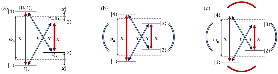
Figure 1: (a) An energy level diagram of a negatively charged quantum dot (QD) in an applied Voigt geometry magnetic field. The degeneracy of the ground and excited eigenstates, written in the basis along the magnetic field axis parallel to the $x$ axis, is lifted by the Zeeman interaction. All four transitions are equally allowed leading to the formation of two $\Lambda$-systems ($1\rightarrow 4\rightarrow 2$ and $2\rightarrow 3\rightarrow 1$). The vertical transitions possess the orthogonal linear polarisation to the diagonal transitions. (b) A $Y$-polarised single-mode cavity coupled to the $Y-$polarised diagonal transitions of a charged-QD in a Voigt geometry magnetic field. (c) A bi-modal cavity with two orthogonal, linearly polarised cavity modes coupled to a charged-QD in a Voigt geometry magnetic field. The line style (solid or compound) and colour indicates the transitions to which the cavity mode couples.

Experiments have demonstrated that the spin states of single electrons confined to quantum dots (QDs) are long-lived [1, 2], with coherence times exceeding $\upmu$s [3, 4], making them promising candidates for an efficient light-matter interface [5]. Furthermore, quantum logic gates may be implemented on ps timescales using ultra-fast optical manipulation of spin-states [3]. Combined, these disparate timescales allow many gate operations to be performed within a single lifetime of the charge state. However, for spin-photon interfaces to be used in optical quantum technologies, such as generating entangled photonic states [6, 7, 8, 9] and spin-photon logic [10, 11] required for many long-range secure quantum network protocols [12, 13], it is necessary to prepare, control, and readout the single spin states with a high fidelity.

Ordinarily, combining optical spin control and read-out requires the use of orthogonal magnetic field geometries: spin control relies on the in-plane Voigt geometry (Fig. 1a) to provide an effective coupling between the spin ground states [14], while read-out uses cycling transitions  in an out-of-plane Faraday field to produce a detectable signal [16]. However, in certain circumstances, spin read-out can be achieved in the Voigt geometry by coupling to a nanophotonic structure [17, 18, 19], which introduces a quasi-cycling transition through a polarisation-dependent Purcell enhancement of the optical transitions.

In this work we investigate the impact single- and bi-modal cavities have on the spin initialisation and readout fidelity for a negatively charged QD in a Voigt geometry magnetic field. We show that, depending on the linewidths and detunings of the cavity modes, a bi-modal cavity may enhance all optical transitions present in a Voigt geometry field, reducing the effectiveness of the quasi-cycling transition. While careful selection of the bi-modal cavity parameters may mitigate these effects, the additional enhancement of the QD transitions result in different cavity parameter requirements for initialisation and readout. Thus, when coupled to a bi-modal cavity we show there is no single set of cavity parameters that simultaneously results in both a good optical initialisation and readout fidelity. Furthermore, we show that single-mode optical cavities outperform bi-modal cavities for both optical initialisation and optical readout across all parameter regimes studied, and can be used to achieve an optimal fidelity in both stages using a single set of cavity parameters.

The paper is organised as follows: in Section II we introduce the background theory for a charged QD interacting with a single- or bi-modal cavity. Sections III and IV investigate how the two cavity configurations impact spin initialisation and readout respectively in isolation. We then discuss the best cavity configurations for initialisation and readout in tandem in Section V.

II Background Theory

In the absence of any applied magnetic fields, a single electron confined to a QD possesses a spin degree of freedom with two degenerate ground states $\{\ket{\uparrow}_{z},\ket{\downarrow}_{z}\}$ defined along the QD growth ($z$) axis, which are chosen to have zero energy. Optically exciting the QD introduces an exciton, forming two negatively charged trion states $\{\ket{\downarrow\uparrow,\Downarrow}_{z},\ket{\uparrow\downarrow,\Uparrow}_{z}\}$ with energy $\hbar\omega_{\mathrm{0}}$. Applying a Voigt geometry magnetic field to the QD lifts the energy degeneracy of both the ground and excited spin states, splitting them by the Zeeman energies $\Delta_{B}^{e}=g_{e}\mu_{B}B$ and $\Delta_{B}^{h}=g_{h}\mu_{B}B$ respectively (Fig. 1a). Here $\mu_{B}$ is the Bohr magneton, $g_{e}$ and $g_{h}$ are the electron and hole effective in-plane g-factors, $B$ is the applied magnetic field strength, and we have ignored any diamagnetic shift. For convenience we redefine the QD spin states in the basis along the magnetic field axis as $\{\ket{1}=\ket{\uparrow}_{x},\ket{2}=\ket{\downarrow}_{x},\ket{3}=\ket{\downarrow\uparrow,\Downarrow}_{x},\ket{4}=\ket{\uparrow\downarrow,\Uparrow}_{x}\}$. Unless otherwise stated, we assume an applied field of $B=5$ T, which yields $\Delta_{\mathrm{B}}^{\mathrm{e}}/2\pi=35$ GHz and $\Delta_{\mathrm{B}}^{\mathrm{h}}/2\pi=20$ GHz, with $g_{\mathrm{e}}=0.5$ and $g_{\mathrm{h}}=0.3$ [20].

In the Voigt geometry, all four transitions become optically allowed with equal magnitude forming two $\Lambda$-systems coupling each excited state to both ground states via two orthogonal, linearly polarised transitions (Fig. 1a). While quasi-cycling transitions are most easily introduced in the Voigt geometry via coupling to a cavity with a single, linearly-polarised mode [21, 22, 23] (Fig. 1b), there are many photonic structures, such as micropillar cavities [24], point-defect PhC cavities [25], crossed nanobeam cavities [26], and open-access microcavities [27], that naturally possess two orthogonal, linearly-polarised modes (Fig. 1c). While such bi-modal cavities have been used to suppress resonant laser background in QD single-photon sources [28, 27], there remain open questions as to the impact on the orthogonally polarised transitions necessary for spin initialisation and readout. Thus in our set-up each of the $\Lambda$-systems transitions can occur through coupling to the free electromagnetic vacuum, or via an optical cavity. The latter is included in the system Hamiltonian $H_{S}=H_{0}+H_{I},$ where in the laboratory frame ($\hbar=1$):

$$H_{0} =\frac{\Delta_{\mathrm{B}}^{\mathrm{e}}}{2}(\sigma_{22}-\sigma_{11})+\left(\omega_{0}-\frac{\Delta_{\mathrm{B}}^{\mathrm{h}}}{2}\right)\sigma_{33}$$

$$+\left(\omega_{0}+\frac{\Delta_{\mathrm{B}}^{\mathrm{h}}}{2}\right)\sigma_{44}+\sum_{\lambda=X,Y}\nu_{\lambda}a^{\dagger}_{\lambda}a_{\lambda}.$$ (1)

Here we have defined the spin operators as $\sigma_{ij}=\ket{i}\!\bra{j}$, and introduced the cavity mode creation (annihilation) operators $a^{\dagger}_{\lambda}$ ($a_{\lambda}$) with frequency $\nu_{\lambda}$, where $\lambda=X,~{}Y,$ denotes the polarisation of the cavity mode. In physical systems the degeneracy of the bi-modal cavity is often lifted either by intentional design [29, 30, 31, 26] or by fabrication imperfections [32, 33], and we therefore assume the cavity modes are detuned.

Applying the rotating wave approximation to our Hamiltonian, the light-matter interaction takes a Jaynes-Cummings form:

$$H_{I}=\sum_{\lambda=X,Y}g_{\lambda}a^{\dagger}_{\lambda}\bm{\sigma}_{\lambda}+g^{\ast}_{\lambda}a_{\lambda}\bm{\sigma}^{\dagger}_{\lambda},$$ (2)

where $g_{\lambda}$ is the light-matter interaction strength for the relevant cavity mode, and we have introduced the collective transition operators $\bm{\sigma}_{X}=\sigma_{14}+\sigma_{23}$ and $\bm{\sigma}_{Y}=\sigma_{24}+\sigma_{13}$ (Fig 1c). With the above definitions, we can recover the single $Y-$polarised mode cavity set-up depicted in Fig. 1b by setting $g_{X}=\nu_{X}=0$.

Spin initialisation and readout necessitate coherent driving of the spin and cavity degrees of freedom respectively. This is included semi-classically in the model via time-dependent driving terms with frequency $\omega_{l}$. This leads to a total Hamiltonian of the form $H_{T}(t)=H_{0}+H_{I}+H_{D}^{QD}(t)+H_{D}^{C}(t)$, where in the dipole and rotating wave approximations the QD driving term may be written as:

$$H_{D}^{QD}(t) =-\frac{1}{2}\sum_{\lambda=X,Y}\Omega_{\lambda}(t)e^{i\omega_{l}t}\bm{\sigma}_{\lambda}+\mathrm{h.c.}.$$ (3)

Here $\Omega_{\lambda}(t)$ is the time-dependent Rabi frequency for the relevant polarisation mode. The cavity driving takes a similar form:

$$H_{D}^{C}(t)=-\sum_{\lambda=X,Y}\epsilon_{\lambda}(t)e^{i\omega_{l}t}a_{\lambda}+\mathrm{h.c.},$$ (4)

where $\epsilon_{\lambda}(t)$ is the time-dependent cavity driving strength. For convenience, we work in a rotating frame with respect to the laser frequency $\omega_{l}$.

In addition to the unitary dynamics generated by the Hamiltonian $H_{\mathrm{T}}(t)$, there are also loss processes acting on the cavity-QD system, namely the emission of photons via the cavity or the electromagnetic vacuum. These are accounted for through a standard Lindblad master equation of the form [34]:

$$\frac{\partial\rho(t)}{\partial t}= -i[H_{T}(t),\rho(t)]$$

$$+\sum_{\lambda=X,Y}\frac{\kappa_{\lambda}}{2}\mathcal{L}_{a_{\lambda}}[\rho(t)]+\frac{\gamma_{\lambda}}{2}\mathcal{L}_{\bm{\sigma}_{\lambda}}[\rho(t)],$$ (5)

where $\rho(t)$ is the reduced density matrix of the cavity-QD system, and $\mathcal{L}_{O}[\rho]=2O\rho O^{\dagger}-\{O^{\dagger}O,\rho\}$ is the Lindblad superoperator. Equation 5 captures the emission of photons in a given polarisation state $\lambda$ via two different channels: the first is leakage from the cavity mode, occurring with a rate $\kappa_{\lambda}$; the second is spontaneous emission directly from the 4-level system (4LS) with rate $\gamma_{\lambda}$. Throughout this paper we shall assume that both polarisation transitions have the same lifetime, such that $\gamma_{\lambda=X,Y}^{-1}=\gamma^{-1}=1$ ns, and in the bi-modal case we assume the cavity modes have identical linewidths ($\kappa_{\lambda=X,Y}=\kappa$) such that $\absolutevalue{g_{X,Y}}=\absolutevalue{g}$ ($g_{X}=g$, $g_{Y}=ig$). The effects of pure dephasing are considered in Appendix A, and are shown to be negligible in most cases. All calculations presented in this paper were performed using the Python package QuTiP [35].

III Spin initialisation

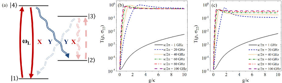
Figure 2: (a) A schematic of the initialisation process. The $\ket{1}\rightarrow\ket{4}$ transition is coherently driven on resonance ($\omega_{l}=\omega_{0}+(\Delta_{B}^{e}+\Delta_{B}^{h})/2$) transferring the spin population to $\ket{2}$ via the $\ket{4}\rightarrow\ket{2}$ transition. Off-resonant driving of the $\ket{2}\rightarrow\ket{3}$ transition returns the spin population to $\ket{1}$. (b), (c) The trace distance between the system steady-state after the initialisation process and the $\ket{2}$ ground state as a function of $g/\kappa$ when coupled to a $Y-$polarised single-mode cavity and a bi-modal cavity respectively. Parameters: $B=$ 5 T, $g_{e(h)}=$ 0.5(0.3), $\gamma^{-1}$ = 1 ns, $\Omega_{X}/2\pi=10^{-3}$ GHz, $\nu_{X}=\omega_{0}$ and $\nu_{Y}=\omega_{0}+(\Delta_{B}^{h}-\Delta_{B}^{e})/2$.

Assuming an initial state with $\rho_{jj}=0.5~{}\mathrm{for}~{}j\in\{1,2\}$ and $\rho_{ij}=0$ otherwise, we wish to prepare the system in the spin state $\ket{2}$ using the protocol presented in [36, 37] and illustrated in Fig. 2a. Initialisation is achieved by resonantly driving the $\ket{1}\rightarrow\ket{4}$ transition using an $X-$polarised laser (i.e. $\Omega_{\mathrm{X}}>0$, $\Omega_{\mathrm{Y}}=0$), such that $\omega_{l}=\omega_{0}+(\Delta_{B}^{e}+\Delta_{B}^{h})/2$. The state $\ket{2}$ is then populated by the diagonal $\ket{4}\rightarrow\ket{2}$ transition. We choose to initialise the spin state by driving the vertical rather than the diagonal transitions as the larger detuning between the vertical transitions relative to the laser bandwidth minimises the off-resonant processes that induce unwanted spin flips away from the $\ket{2}$ target state.

To quantify the initialisation fidelity we use the trace distance, $T(\rho,\varrho)=\frac{1}{2}\Tr{\sqrt{(\rho-\varrho)^{2}}}$, between the prepared ($\rho$) and target ($\varrho$) states [38]. The trace distance provides a measure of the distinguishability of two given states using the entirety of the density matrix including all state populations and coherences. For the pure target state used in this case ($\varrho=\sigma_{22}$) this definition is equivalent to the fidelity used in other studies [19, 20, 39]. However, it may not always be the case that a pure state is the desired outcome of the initialisation process. Hence we have opted to use the more general trace distance as this is often simpler to calculate and provides a true metric on density matrix space, naturally distinguishing between coherent superposition and mixed spin states which would be overlooked if relative spin populations were used as a measure of preparation fidelity [36, 40, 41, 42]. Using this metric, $T(\rho=\sigma_{22},\sigma_{22})=0$ indicates the prepared state is indistinguishable from the target state (unity initialisation fidelity). Conversely, $T(\rho,\sigma_{22})=1$ indicates the prepared state is orthogonal to the target state, and is therefore completely distinguishable.

For both the single and bi-modal cavity configurations we choose the $Y$-polarised mode to be resonant with the $\ket{2}\rightarrow\ket{4}$ transition (i.e. $\nu_{Y}=\omega_{0}+(\Delta_{B}^{h}-\Delta_{B}^{e})/2$). However, when coupled to a bi-modal cavity we leave the $X-$polarised cavity mode detuned from the vertical transitions such that $\nu_{X}=\omega_{0}$ as this has been shown to maximise the initialisation fidelity with this cavity configuration [36].

To allow a direct comparison between the two cavity configurations, we assume spin initialisation is achieved by directly driving the QD transitions. This differs to previous work studying spin initialisation with bi-modal cavities, which use cavity driving rather than direct QD driving to initialise the spin state [36]. However, both schemes lead to qualitatively the same behaviour, and importantly considering only one driving configuration allows a fair and consistent comparison between the individual cavity set-ups .

III.1 Steady-State Limit

Using the model in Sec. II, we begin by studying initialisation in the steady-state limit with a continuous wave (CW) driving term (i.e. $\Omega_{X}(t)~{}=~{}\Omega_{X}~{}\forall~{}t$). While this limit does not accurately reflect experimental procedures for initialising spin states, the steady-state still provides an insight into the behaviour of the system and limits the available parameter space. Figures 2b and 2c show the calculated trace distance between the prepared steady-state and target state with a fixed driving strength as a function of $g/\kappa$ for a range of cavity linewidths.

The results presented in Fig. 2 show that in the steady-state limit the inclusion of cavity effects reduces the initialisation fidelity. For small $g$ this is a result of the cavity modifying lifetime of the trion states, and thus the ratio $\Omega/\gamma$. As the cavity coupling strength is increased the fixed driving strength is no longer optimised to achieve the smallest trace distance. We therefore find that for each set of cavity parameters the Rabi frequency needs to be optimised to minimise the trace distance. As the cavity-coupled system enters the strong coupling regime ($g\gg\kappa,\gamma$) the QD states hybridise with the cavity modes, fundamentally changing the system eigenstructure, which leads to a maximally mixed ground state, where $T(\rho,\sigma_{11})=T(\rho,\sigma_{22})=0.5$. For a bi-modal cavity set-up we find the steady-state evolves to return $0.1\leq T(\rho,\sigma_{22})\leq 0.5$ depending on the cavity linewidth.

In the limit of the narrowest cavity linewidths, we expect both cavity configurations to display similar behaviour. At these linewidths only the $\ket{4}\rightarrow\ket{2}$ transition experiences a significant Purcell enhancement in either cavity configuration, with all other optical transitions sufficiently detuned from the cavity mode to experience little to no enhancement. This expectation is borne out in Fig. 2 with $\kappa/2\pi=1$ GHz. At this cavity linewidth both cavity configurations return similar trace distances, with small differences resulting from some non-zero enhancement of the $X-$polarised transitions when coupled to a bi-modal cavity.

With large coupling strengths, we find the bi-modal cavity outperforms the single-mode cavity, returning smaller trace distances for $1~{}\mathrm{GHz}~{}<\kappa/2\pi<100$ GHz. At intermediate cavity linewidths, the Purcell enhancement of the $\ket{3}\rightarrow\ket{2}$ transition is greater than that of the $\ket{3}\rightarrow\ket{1}$ transition. Thus any population in the $\ket{3}$ state excited through off-resonant driving will preferentially decay back to the desired $\ket{2}$ state, providing additional protection to the prepared state. While the Purcell enhancement of the $\ket{4}\rightarrow\ket{1}$ transition does hinder the initialisation process, this effect is less significant in the limit of infinite driving time. Increasing the cavity linewidth begins to equalise the enhancement of the transitions away from the $\ket{3}$ state, hence the system tends towards the maximally mixed ground state with $T(\rho,\sigma_{22})=0.5$ as in the single-mode case.

III.2 Finite Pulse Duration

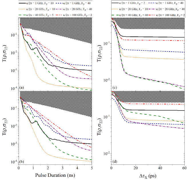
Figure 3: The trace distances after the initialisation process as a function of: (left: a,b) the duration of the square driving pulse minimised with respect to the Rabi frequency and (right: c,d): the FWHM of the Gaussian driving pulse minimised with respect the pulse area when coupled to (top: a,c) a single mode cavity, and (bottom: b,d) a bi-modal cavity. The trace distances were calculated for a number of cavity parameter combinations given in the legends above the relevant plots. Note the left and right plots use different scales for the trace distance. The Rabi frequency was swept between $0\leq\Omega_{X}\leq 10\gamma$, and similarly for the Gaussian pulse the pulse area was swept between $0.01\pi\leq\Theta_{X}\leq 5\pi$. The shaded regions indicate trace distances larger than those achievable in the absence of any cavity effects when driving the QD with the respective pulse types. Parameters: $B=$ 5 T, $g_{e(h)}=$ 0.5(0.3), $\gamma^{-1}$ = 1 ns, $\nu_{X}=\omega_{0}$, and $\nu_{Y}=\omega_{0}+(\Delta_{B}^{h}-\Delta_{B}^{e})/2$.

While the limit of infinite driving time provides some insight into the system behaviours, it does not accurately reflect the experimental realisation of optical spin initialisation. Any experimentally relevant protocol requires the initialisation process to occur in a finite time, and is thus achieved with finite optical pulses rather than CW drive. Maximising the spin initialisation fidelity in this limit of finite driving time requires maximising the efficiency and speed with which the spin population is transferred from the $\ket{1}$ state to the $\ket{2}$ state. Thus we now consider the impact of cavity coupling on the initialisation of the spin system when driven by a finite optical pulse with either a square or Gaussian envelope.

As pulsed optical driving is a more accurate representation of the experimental realisation of optical spin initialisation, we now opt to calculate $T(\varrho,\sigma_{22})$ as a function of more experimentally accessible parameters, namely the Purcell factor and cavity linewidth. The combination of the light-matter coupling strength and cavity linewidth leads to an enhanced emission rate from the relevant optical transition quantified through the Purcell enhancement $F_{P}(\lambda)=4|g_{\lambda}|^{2}/\kappa_{\lambda}\gamma_{\lambda}$ when on resonance [25]. We shall restrict the cavity linewidth and Purcell factor to $1\leq\kappa/2\pi\leq 110$ GHz and $1\leq F_{P}\leq 40$ respectively. This maintains the Purcell enhancement in a regime that has been experimentally demonstrated [25], and limits the cavity quality factors to experimentally achievable values (on the order of $10^{3}-10^{5}$ for wavelengths in the NIR and telecommunications bands).

III.2.1 Square Pulse

We first examine initialisation with a finite square pulse with $\Omega_{X}(t)=\Omega(H(t-t_{0}+\Delta\tau_{X}/2)-H(t-t_{0}-\Delta\tau_{X}/2))$, where $H(x)$ is the Heaviside function, $t_{0}$ is the centre of the pulse, $\Delta\tau_{X}$ is the pulse duration, and $\Omega$ is the Rabi frequency of the pulse. For a given set of cavity parameter combinations, we vary the Rabi frequency of the pulse in the range $0\leq\Omega_{X}\leq 10\gamma$ to find the minimum trace distance for each pulse duration $\Delta\tau_{X}$, leaving adequate time after the pulse for the trion populations to fully decay. Figures 3a and 3b show the resulting minimised trace distance as a function of pulse duration for the single- and bi-modal cavities respectively. The effects of pure dephasing are discussed in Appendix A, and are shown to have similarly negligible effects for either cavity configuration when driving with a square pulse.

Irrespective of cavity configuration, we find a general trend of decreasing trace distance with increasing pulse duration. Longer pulse durations both increase the fraction of the $\ket{1}$ state population transferred to the excited state, and, when the pulse duration is longer than the excited state lifetime, enable the re-excitation of any non-zero $\ket{1}$ population resulting from the decay of the trion states via the $\ket{4}\rightarrow\ket{1}$ and $\ket{3}\rightarrow\ket{1}$ transitions. Furthermore, increasing the duration of the driving pulse decreases its bandwidth which in turn reduces the strength of the off-resonant driving of the $\ket{2}\rightarrow\ket{3}$ transition that moves the system away from the target state.

When coupled to a single-mode cavity and driving with a square pulse (Fig. 3a), we find the Purcell enhancement of the resonant diagonal transition is the most important factor in achieving a high initialisation fidelity. For the majority of the cavity parameter combinations studied, the effect of the cavity linewidth only becomes significant at longer pulse durations, depending on the Purcell factor. Figure 3a shows that neither the largest Purcell factor nor the narrowest cavity linewidth studied necessarily produces the best fidelity in the limit of finite pulse duration. Instead, of the cavity parameter combinations studied, an intermediate linewidth of $\kappa/2\pi=20$ GHz and Purcell factor of $F_{P}=10$ produced the smallest trace distance over the largest range of pulse durations. Maximising the initialisation fidelity requires balancing the rates at which the system is driven to and from the target state. An intermediate cavity linewidth is required to avoid the cyclical re-excitation of the $\ket{4}$ state that would occur in the strong coupling regime, and act to increase $T(\varrho,\sigma_{22})$. However, to limit the rate at which the system is driven away from the target $\ket{2}$ state owing to the increased spectral bandwidth of the finite pulse, the Purcell factor must also be limited to minimise the decay rate of the unwanted $\ket{3}\rightarrow\ket{1}$ transition.

Similar results are found when the QD is coupled to a bi-modal cavity (Fig. 3b). Again the Purcell enhancement of the resonant diagonal transition appears to be the dominant factor in determining the trace distance as a function of pulse duration. However, relative to initialisation with a single-mode cavity, the calculated trace distances are larger and require a longer pulse duration to achieve. In this configuration, we find a Purcell factor of $F_{P}=40$ produces the largest trace distances for the majority of cavity linewidths studied. For the cavity parameters considered, we find that $F_{P}=10$ and $\kappa/2\pi=1$ GHz produces the best initialisation fidelity with pulse durations less than $\approx 0.5$ ns while $F_{P}=10$ and $\kappa/2\pi=20$ GHz produces the best initialisation fidelity for pulse durations greater than $\approx 0.5$ ns.

Plateaus in the trace distance can also be seen in Figs. 3a and 3b. These plateaus are artifacts of limiting range over which the Rabi frequency is swept for each data point. Driving the system with increasing Rabi frequency naturally results in Rabi oscillations in the system populations. The edge of each plateau occurs when the pulse duration is long enough to encompass the next oscillation with a lower local minimum than the previous. These plateaus are not seen at longer pulse durations as the global minimum in the trace distance as a function of Rabi frequency usually occurs after two or three oscillations.

III.2.2 Gaussian Pulse

We now move on to study initialisation with a Gaussian optical pulse. We define the Gaussian pulse with polarisation $\lambda=X,Y$ centered around $t_{0}$ as:

$$\Omega_{\lambda}(t)=\frac{\Theta_{\lambda}}{\sqrt{2\pi w_{\lambda}^{2}}}\exp\left\{{-\frac{\left(t-t_{0}\right)^{2}}{2w_{\lambda}^{2}}}\right\},$$ (6)

where $\Theta_{\lambda}=\int_{-\infty}^{\infty}dt\Omega_{\lambda}(t)$ is the pulse area defined such that a pulse with $\Theta_{\lambda}=\pi$ would invert the population of a two-level system, and $w_{\lambda}$ is the Gaussian width of the pulse related to the intensity Full-Width Half-Maximum ($\Delta\tau_{\lambda}$) by:

$$w_{\lambda}=\frac{\Delta\tau_{\lambda}}{2\sqrt{\ln{2}}}.$$ (7)

Following the procedure for the finite square pulse, we plot the trace distance, minimised with respect to the pulse area in the range $0.01\pi\leq\Theta_{X}\leq 5\pi$, as a function of $\Delta\tau_{X}$. Figures 3c and 3d show the results for the single- and bi-modal set-ups respectively.

Just as with the square optical pulse, we find the trace distance decreases with increasing pulse duration. From Figs. 3c and 3d it is clear that spin initialisation with Gaussian pulses occurs on much shorter timescales than when using square pulses, with the trace distance being optimised in tens of picoseconds rather than a few nanoseconds. Additionally, the trace distances achieved with a Gaussian pulse are smaller than those achieved with the shortest square pulses studied ($<1$ ns) which are unlikely to be experimentally accessible. However, the smallest achieved trace distances driving with a Gaussian pulse are orders of magnitude larger than those found when driving with a longer square pulse ($>1$ ns). Below $\Delta\tau_{X}\lessapprox 15$ ps this is a consequence of the bandwidth of the driving pulse resulting in a significant spectral overlap between the driving field and the off-resonant $\ket{2}\rightarrow\ket{3}$ vertical transition, which in turn increases the driving of the system away from the desired state. However, beyond $\Delta\tau_{X}\approx 15$ ps this overlap is minimised, and thus the trace distance is governed by re-excitation of population that initially decayed into the unwanted ground state ($\ket{1}$). This in turn is limited by the ratio of the decay rate of the trion states into the $\ket{1}$ state and the pulse duration. Furthermore, attaining these trace distances when driving with a Gaussian pulse requires the largest Purcell enhancement for all but the narrowest cavity linewidths due to the pulse duration being much shorter than the trion lifetimes, which can prove challenging to realise experimentally.

We again find coupling the QD to a bi-modal cavity significantly increases the calculated trace distances after the initialisation procedure. In fact, for some of the cavity parameters studied for the bi-modal case, the produced trace distances are comparable to initialisation with a Gaussian pulse in the absence of any cavity effects. However, Appendix A shows that when driving with a Gaussian pulse, spin initialisation with a bi-modal cavity configuration is the most robust against pure dephasing.

IV Spin Readout

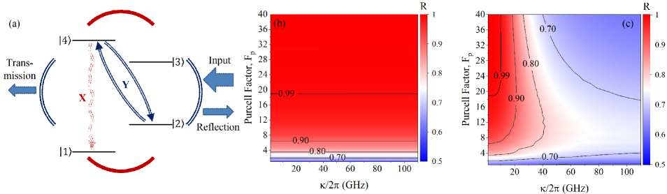
Figure 4: (a) A diagram of the spin-readout process. The $Y$-polarised cavity mode is probed with a square laser pulse and the QD-state dependent reflectivity/transmissivity is measured. By comparing the collected photon number with a threshold value the spin state of the system may be determined. (b) and (c) The calculated readout fidelities ($R$) for a single mode cavity, and a bi-modal cavity respectively, when driving the $Y-$polarised cavity mode with a 35 ns square pulse. Parameters: $B=$ 5 T, $g_{e(h)}=$ 0.5(0.3), $\gamma^{-1}$ = 1 ns, $\epsilon_{Y}=\sqrt{(0.01\times 2g_{Y}^{2})}$, $\eta=1$, $\nu_{X}=\omega_{0}$ and $\nu_{Y}=\omega_{0}+(\Delta_{B}^{h}-\Delta_{B}^{e})/2$.

In addition to high fidelity spin initialisation, it is crucial that the cavity structures are also conducive to high fidelity readout. We therefore study optical spin readout for both single mode and bi-modal cavities using the method first proposed in [17], and demonstrated experimentally in [18]. This readout method uses the spin-dependent transmissivity or reflectivity of a cavity mode resonantly coupled to a transition of the QD to determine its spin state. In contrast to Ref. [17], we choose the cavity configuration to mirror the set-up used for high-fidelity spin initialisation, where the cavity mode is coupled to the diagonal transitions. The diagonal $\ket{2}\rightarrow\ket{4}$ transition is then weakly probed by a resonant drive via the $Y-$polarised cavity mode present in either cavity configuration. If the emitter occupies the $\ket{1}$ state the photons are transmitted, while if the QD resides in the $\ket{2}$ state the photons are reflected (see Fig. 4a). By comparing the ratio of photons transmitted versus incident with a threshold value [17], the state ($\ket{1}$ or $\ket{2}$) occupied by the QD can be determined.

The readout protocol is initialised by weakly probing the $Y$-polarised cavity mode over some time-interval $[0,\tau]$, where $\tau$ is much longer than the lifetime of the system. Over this time interval, we set a threshold photon number $k$, where if the number of collected transmitted photons is less than $k$ then the qubit state is $\ket{2}$, otherwise it is $\ket{1}$. The maximum probability of a successful readout occurring is then given by $\mathcal{R}=\max_{k}(q_{1}p_{1}(k)+q_{2}p_{2}(k))$, where $q_{i}$ is the probability of finding the qubit in state $i$, and $p_{i}$ is the probability of getting a correct result using threshold photon number $k$. As shown by Ref. [17], for detectors with a dead time shorter than the interval between detection events, and in the weak driving limit, the probabilities $p_{i}(k)$ can be described by Poissonian statistics. This allows the readout fidelity ($\mathcal{R}$) to be written as [17]:

$$\mathcal{R}(\tau)=\frac{1}{2}-\frac{1}{2}\sum_{k=0}^{M}\frac{1}{k!}\Bigl{(}\left[N_{1}(\tau)\right]^{k}e^{-N_{1}(\tau)}\\ -\left[N_{2}(\tau)\right]^{k}e^{-N_{2}(\tau)}\Bigr{)},$$ (8)

where $M$ is the optimal threshold value [17]:

$$M=\left\lfloor\frac{N_{2}(\tau)-N_{1}(\tau)}{\ln\left[N_{2}(\tau)\right]-\ln\left[N_{1}(\tau)\right]}\right\rfloor,$$ (9)

with $\lfloor x\rfloor$ indicating the largest integer smaller than x, and $N_{i}$ is the number of photons emitted from the cavity mode when the QD starts in the ground state $\ket{i=1,2}$. The number of photons emitted can be found by integrating the output flux of the cavity over the duration of the optical readout pulse [17]:

$$N_{i,\lambda}(\tau)=\eta\int_{0}^{\tau}\left|\Tr\left[\sqrt{\kappa_{\lambda}}a_{\lambda}\rho_{i}(t)\right]\right|^{2}dt.$$ (10)

Here $\tau$ is the duration of the readout pulse, $\eta$ is the photon collection efficiency, and $\rho_{i}(t)$ are the density matrices of the system at time $t$ when the QD is initialised in the ground state $\ket{i=1,2}$. We also continue to assume both modes of the bi-modal cavity have identical linewidths such that $\kappa_{\lambda=X,Y}=\kappa$. This readout method has been demonstrated to work experimentally, producing $\mathcal{R}=0.61$ with a cavity linewidth $\kappa/2\pi=67$ GHz, an enhancement factor $F_{P}=62$, a collection efficiency $\eta=4.1\times 10^{-3}$, and 75 ns pulse duration [18].

Considering a square pulse with a duration of $35$ ns , and time-dependent cavity driving strength $\epsilon_{Y}(t)=\sqrt{(0.01\times 2g_{Y}^{2})}$ for $t\in[0,35~{}\mathrm{ns}]$ to remain in the weak-excitation regime [17], and assuming $\eta=1$, we calculate the spin readout fidelity for a range of cavity parameters. Fig. 4b and Fig. 4c show these results for a single-mode and bi-modal cavity respectively. In the case of the single-mode cavity, we find the readout fidelity is primarily dependent on the Purcell enhancement of the diagonal transitions, and varies little with respect to $\kappa_{Y}$. This is because the Purcell enhancement increases the strength of the quasi-cycling transition required to produce a detectable readout signal, while the cavity linewidth has little impact on the Purcell enhancement of the resonant transition being probed. Figure 4b shows $F_{P}=7$ gives $\mathcal{R}>90\%$ and $F_{P}=19$ gives $\mathcal{R}>99\%$.

In contrast, the bi-modal readout fidelity is sensitive to both the cavity linewidth and Purcell enhancement of the optical transitions. The highest readout fidelities with this cavity configuration are produced with narrow cavity linewidths and large Purcell factors. The narrow cavity linewidths ensure the vertical transitions, detuned from the cavity resonance, are not Purcell enhanced. This increases the cyclicity of the $\Lambda$-systems, which naturally increases the strength of the quasi-cycling transition probed during the readout procedure. To achieve $\mathcal{R}>99\%$ with a bi-modal cavity requires $\kappa/2\pi\leq 9.4$ GHz and $F_{P}\geq 19$. Note that under these driving conditions, when the cavity parameters are optimised for either cavity configuration, we find that a collection efficiency of $\eta\geq 48\%$ gives $\mathcal{R}\geq 99\%$. Such collection efficiencies have already been demonstrated in an open-access microcavity system [27]; for planar PhC or nanobeam structures very high efficiencies could be achieved by direct fibre coupling [45, 46]. The effects of pure dephasing on the readout fidelity are shown in Appendix A. We find that, while increasing the pure dephasing rate increases the required Purcell factors for both cavity configurations, the single-mode cavity is more robust against these processes in the readout stage.

V Conclusion

By performing full cavity QED calculations, we have investigated optical spin initialisation and readout for a QD interacting with either single- or bi-modal optical cavities. Interestingly, we find that for both initialisation and readout, a single mode optical cavity outperforms the bi-modal cavity over the full parameter regime studied regardless of the pulse envelope used. This is a consequence of the bi-modal cavity Purcell enhancing undesirable transitions, therefore suppressing desired spin-flip processes. While these unwanted transitions can be suppressed for spin preparation, we find that they restrict the parameter regimes for which high fidelity optical spin readout can be achieved with bi-modal cavities. Furthermore, this range of optimal readout cavity parameters (large $F_{P}$) does not overlap with the small range of cavity parameters required for optimised spin initialisation in a bi-modal cavity (small $F_{P}$).

In contrast, we have shown a near unity readout fidelity is possible with a single-mode cavity across the vast majority of the cavity parameters studied. In the single mode configuration with experimentally achievable [47, 48, 49] cavity parameters ($\kappa/2\pi=20$ GHz, $F_{P}=10$), we find an initialisation trace distance $T(\rho,\sigma_{22})=1.3\times 10^{-4}$ is achievable with a 3 ns square optical pulse, whilst a readout success probability of $\mathcal{R}=0.95$ is possible with a 35 ns optical pulse. Increasing the Purcell factor to $F_{P}=19$ increases the readout success rate to $\mathcal{R}=0.99$ while maintaining an initialisation trace distance on the order of $10^{-4}$. For a bi-modal system using the same parameters, a comparable initialisation trace distance of $T(\rho,\sigma_{22})=2.2\times 10^{-4}$ is achievable. However, the corresponding readout success rate is reduced to $\mathcal{R}=0.88$. In the parameter regimes studied here, no single set of bi-modal cavity parameters simultaneously allow for high fidelity spin initialisation and readout with finite optical pulses.

These results suggest that to realise a high fidelity spin-photon interface, a single linearly-polarized cavity mode providing a modest ($\sim 20$) Purcell enhancement is the optimal configuration. In addition, further calculations presented in Appendix A demonstrate that this parameter regime is also robust against significant levels of pure dephasing, illustrating the potential to achieve high performance spin-photon interfaces in real physical systems. For inherently bi-modal cavities such as micropillars or point-defects in PhCs, our analysis suggests that there would be significant benefit in modifying designs to induce a mode splitting much larger than the cavity linewidth (e.g. elliptical micropillars [28]). We believe that these insights and methods will contribute to the development of high fidelity spin-photon interfaces that meet the stringent requirements of future optical quantum technologies.

VI Acknowledgements

The authors would like to acknowledge the funding support of the University of Sheffield, and EPSRC grants EP/N031776/1 and EP/V026496/1. For the purpose of open access, the authors have applied a Creative Commons Attribution (CC BY) license to any Author Accepted Manuscript version arising.

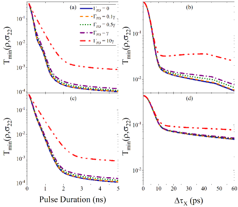
Figure 5: The calculated trace distance between the state prepared by the initialisation process and the target state minimising with respect to the driving strength when driving with a (left: a,c) Square pulse or (right: b,d) Gaussian pulse, and coupled to a (top: a,b) single-mode or (bottom: c,d) bi-modal cavity for different pure dephasing rates indicated in the legend in (a) using the cavity parameters that minimise the trace distance in the absence of pure dephasing processes. Parameters used: $\gamma^{-1}$ = 1 ns, (a,c) $\kappa/2\pi=20$ GHz, $F_{P}=10$, (b) $\kappa/2\pi=40$ GHz, $F_{P}=40$, (d) $\kappa/2\pi=20$ GHz, $F_{P}=40$.

Appendix A Pure Dephasing

Thus far we have assumed that the trion states are lifetime limited. However, in physical systems elastic processes will occur that preserve the spin populations, but reduce their coherence. We therefore also study the effect of pure dephasing of the trion states on the spin initialisation and readout processes when driving with a finite duration pulse. We account for pure dephasing through the addition of further Lindblad terms,

$$\sum_{j=3,4}\frac{\Gamma}{2}\mathcal{L}_{\bm{\sigma}_{jj}}[\rho(t)],$$ (11)

in the master equation. Here $\Gamma$ is the pure dephasing rate, and $\mathcal{L}_{O}[\rho]=2O\rho O^{\dagger}-\{O^{\dagger}O,\rho\}$ is the Lindblad super-operator.

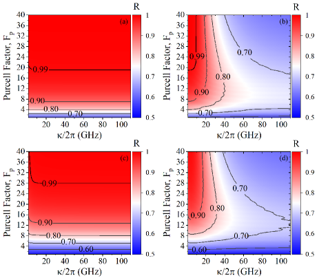
Figure 6: The calculated spin readout success probabilities when coupled to a (left: a,c) single-mode or (right: b,d) bi-modal cavity when the 4LS experiences pure dephasing with rates (top: a,b) $\Gamma=\gamma$ and (bottom: c,d) $\Gamma=10\gamma$. Parameters used: $B=$ 5 T, $g_{e(h)}=$ 0.5(0.3), $\gamma^{-1}$ = 1 ns, $\epsilon_{Y}=\sqrt{(0.01\times 2g_{Y}^{2})}$, $\eta=1$, $\nu_{X}=\omega_{0}$ and $\nu_{Y}=\omega_{0}+(\Delta_{B}^{h}-\Delta_{B}^{e})/2$.

A.1 Spin Initialisation

To study the influence of pure dephasing in the optical initialisation process we follow the same procedure presented in Sec. III, sweeping the duration of the given optical pulse and minimising the trace distance with respect to the Rabi frequency or pulse area. However, we now only consider the combination of cavity parameters that produced the smallest trace distance in the absence of pure dephasing for a given pulse envelope, and instead plot the calculated trace distances for a number of pure dephasing rates.

Figure 5 shows that when $\Gamma\leq\gamma$ pure dephasing has a minimal impact on the calculated trace distances after the initialisation process for any combination of driving pulse envelope and cavity configuration. For $\Gamma\gg\gamma$, Fig. 5 shows pure dephasing significantly increases the calculated trace distances. For all combinations studied the divergence between the traces distances calculated neglecting and including pure dephasing increases with increasing pulse duration. However, while producing the largest minimised trace distance, optical spin initialisation with the combination of a bi-modal cavity and Gaussian pulse drive appears the least susceptible to the influence of pure dephasing. The Purcell enhancement of all four optical transitions, combined with the fast optical driving, work to reduce the relative impact of pure dephasing mechanisms by minimising the time the system spends in the excited states. Nevertheless, we note that for all configurations, small trace distances are achievable even in the presence of significant pure dephasing.

A.2 Spin Readout

To study the impact of pure dephasing on the spin readout process we calculate the readout success probability for two pure dephasing rates, $\Gamma=\gamma$ and $\Gamma=10\gamma$. Figure 6 shows the results when coupled to a single-mode or bi-modal cavity. When coupled to a single-mode cavity, Figs. 6(a) and (c) show the readout process is robust against pure dephasing mechanisms. Even at the largest pure dephasing rate studied, $\mathcal{R}>99\%$ remains achievable for a large range of cavity linewidths albeit at a larger threshold Purcell factors compared with $\Gamma=0$ (Fig. 4). However, while a similar result is found for $\Gamma=\gamma$ when the 4LS is coupled to a bi-modal cavity, at $\Gamma=10\gamma$ we find no bi-modal cavity parameter combinations that can produce $\mathcal{R}>99\%$.

References

- Kroutvar et al. [2004] M. Kroutvar, Y. Ducommun, D. Heiss, M. Bichler, D. Schuh, G. Abstreiter, and J. J. Finley, Optically programmable electron spin memory using semiconductor quantum dots, Nature 432, 81 (2004).
- Gillard et al. [2021] G. Gillard, I. M. Griffiths, G. Ragunathan, A. Ulhaq, C. McEwan, E. Clarke, and E. A. Chekhovich, Fundamental limits of electron and nuclear spin qubit lifetimes in an isolated self-assembled quantum dot, npj Quantum Information 7, 1 (2021).
- Press et al. [2010] D. Press, K. De Greve, P. L. McMahon, T. D. Ladd, B. Friess, C. Schneider, M. Kamp, S. Höfling, A. Forchel, and Y. Yamamoto, Ultrafast optical spin echo in a single quantum dot, Nature Photonics 4, 367 (2010).
- Bechtold et al. [2015] A. Bechtold, D. Rauch, F. Li, T. Simmet, P.-L. Ardelt, A. Regler, K. Müller, N. A. Sinitsyn, and J. J. Finley, Three-stage decoherence dynamics of an electron spin qubit in an optically active quantum dot, Nature Physics 11, 1005 (2015).
- Kimble [2008] H. J. Kimble, The quantum internet, Nature 453, 1023 (2008).
- Lindner and Rudolph [2009] N. H. Lindner and T. Rudolph, Proposal for pulsed on-demand sources of photonic cluster state strings, Phys. Rev. Lett. 103, 113602 (2009).
- Denning et al. [2017] E. V. Denning, J. Iles-Smith, D. P. McCutcheon, and J. Mork, Protocol for generating multiphoton entangled states from quantum dots in the presence of nuclear spin fluctuations, Physical Review A 96, 062329 (2017).
- Scerri et al. [2018] D. Scerri, R. N. E. Malein, B. D. Gerardot, and E. M. Gauger, Frequency-encoded linear cluster states with coherent raman photons, Phys. Rev. A 98, 022318 (2018).
- Schwartz et al. [2016] I. Schwartz, D. Cogan, E. R. Schmidgall, Y. Don, L. Gantz, O. Kenneth, N. H. Lindner, and D. Gershoni, Deterministic generation of a cluster state of entangled photons, Science 354, 434 (2016).
- Sun et al. [2016] S. Sun, H. Kim, G. S. Solomon, and E. Waks, A quantum phase switch between a single solid-state spin and a photon, Nature Nanotechnology 11, 539 (2016).
- Sun et al. [2018a] S. Sun, H. Kim, Z. Luo, G. S. Solomon, and E. Waks, A single-photon switch and transistor enabled by a solid-state quantum memory, Science 361, 57 (2018a).
- Borregaard et al. [2020] J. Borregaard, H. Pichler, T. Schröder, M. D. Lukin, P. Lodahl, and A. S. Sørensen, One-way quantum repeater based on near-deterministic photon-emitter interfaces, Phys. Rev. X 10, 021071 (2020).
- Munro et al. [2012] W. J. Munro, A. M. Stephens, S. J. Devitt, K. A. Harrison, and K. Nemoto, Quantum communication without the necessity of quantum memories, Nature Photonics 6, 777 (2012).
- Atatüre et al. [2006] M. Atatüre, J. Dreiser, A. Badolato, A. Högele, K. Karrai, and A. Imamoglu, Quantum-dot spin-state preparation with near-unity fidelity, Science 312, 551 (2006).
- Note [1] Cycling transitions are transitions that always return the system to the same ground state [50].
- Delteil et al. [2014] A. Delteil, W.-b. Gao, P. Fallahi, J. Miguel-Sanchez, and A. Imamoğlu, Observation of quantum jumps of a single quantum dot spin using submicrosecond single-shot optical readout, Phys. Rev. Lett. 112, 116802 (2014).
- Sun and Waks [2016] S. Sun and E. Waks, Single-shot optical readout of a quantum bit using cavity quantum electrodynamics, Phys. Rev. A 94, 012307 (2016).
- Sun et al. [2018b] S. Sun, H. Kim, G. S. Solomon, and E. Waks, Cavity-enhanced optical readout of a single solid-state spin, Phys. Rev. Applied 9, 054013 (2018b).
- Appel et al. [2021] M. H. Appel, A. Tiranov, A. Javadi, M. C. Löbl, Y. Wang, S. Scholz, A. D. Wieck, A. Ludwig, R. J. Warburton, and P. Lodahl, Coherent spin-photon interface with waveguide induced cycling transitions, Phys. Rev. Lett. 126, 013602 (2021).
- Emary et al. [2007] C. Emary, X. Xu, D. G. Steel, S. Saikin, and L. J. Sham, Fast initialization of the spin state of an electron in a quantum dot in the voigt configuration, Phys. Rev. Lett. 98, 047401 (2007).
- Arcari et al. [2014] M. Arcari, I. Söllner, A. Javadi, S. Lindskov Hansen, S. Mahmoodian, J. Liu, H. Thyrrestrup, E. H. Lee, J. D. Song, S. Stobbe, and P. Lodahl, Near-unity coupling efficiency of a quantum emitter to a photonic crystal waveguide, Phys. Rev. Lett. 113, 093603 (2014).
- Reinhard et al. [2012] A. Reinhard, T. Volz, M. Winger, A. Badolato, K. J. Hennessy, E. L. Hu, and A. Imamoğlu, Strongly correlated photons on a chip, Nature Photonics 6, 93 (2012).
- Ohta et al. [2011] R. Ohta, Y. Ota, M. Nomura, N. Kumagai, S. Ishida, S. Iwamoto, and Y. Arakawa, Strong coupling between a photonic crystal nanobeam cavity and a single quantum dot, Applied Physics Letters 98, 173104 (2011).
- Reithmaier et al. [2004] J. P. Reithmaier, G. Sęk, A. Löffler, C. Hofmann, S. Kuhn, S. Reitzenstein, L. V. Keldysh, V. D. Kulakovskii, T. L. Reinecke, and A. Forchel, Strong coupling in a single quantum dot-semiconductor microcavity system, Nature 432, 197 (2004).
- Liu et al. [2018] F. Liu, A. J. Brash, J. O’Hara, L. M. P. P. Martins, C. L. Phillips, R. J. Coles, B. Royall, E. Clarke, C. Bentham, N. Prtljaga, I. E. Itskevich, L. R. Wilson, M. S. Skolnick, and A. M. Fox, High purcell factor generation of indistinguishable on-chip single photons, Nature Nanotechnology 13, 835 (2018).
- Rivoire et al. [2011] K. Rivoire, S. Buckley, and J. Vučković, Multiply resonant high quality photonic crystal nanocavities, Applied Physics Letters 99, 013114 (2011).
- Tomm et al. [2021] N. Tomm, A. Javadi, N. O. Antoniadis, D. Najer, M. C. Löbl, A. R. Korsch, R. Schott, S. R. Valentin, A. D. Wieck, A. Ludwig, and R. J. Warburton, A bright and fast source of coherent single photons, Nature Nanotechnology 16, 399 (2021), 2007.12654 .
- Wang et al. [2019] H. Wang, Y.-M. He, T.-H. Chung, H. Hu, Y. Yu, S. Chen, X. Ding, M.-C. Chen, J. Qin, X. Yang, et al., Towards optimal single-photon sources from polarized microcavities, Nature Photonics 13, 770 (2019).
- Coles et al. [2014] R. J. Coles, N. Prtljaga, B. Royall, I. J. Luxmoore, A. M. Fox, and M. S. Skolnick, Waveguide-coupled photonic crystal cavity for quantum dot spin readout, Optics Express 22, 2376 (2014).
- Gür et al. [2021] U. M. Gür, M. Mattes, S. Arslanagić, and N. Gregersen, Elliptical micropillar cavity design for highly efficient polarized emission of single photons, Applied Physics Letters 118, 10.1063/5.0041565 (2021).
- Gayral et al. [1998] B. Gayral, J. M. Gérard, B. Legrand, E. Costard, and V. Thierry-Mieg, Optical study of GaAs/AlAs pillar microcavities with elliptical cross section, Applied Physics Letters 72, 1421 (1998).
- Reitzenstein et al. [2007] S. Reitzenstein, C. Hofmann, A. Gorbunov, M. Strauß, S. H. Kwon, C. Schneider, A. Löffler, S. Höfling, M. Kamp, and A. Forchel, Alas gaas micropillar cavities with quality factors exceeding 150.000, Applied Physics Letters 90, 251109 (2007).
- Luxmoore et al. [2012] I. J. Luxmoore, E. D. Ahmadi, B. J. Luxmoore, N. A. Wasley, A. I. Tartakovskii, M. Hugues, M. S. Skolnick, and A. M. Fox, Restoring mode degeneracy in h1 photonic crystal cavities by uniaxial strain tuning, Applied Physics Letters 100, 121116 (2012).
- Carmichael [1999] H. J. Carmichael, Statistical methods in quantum optics 1: master equations and Fokker-Planck equations, Vol. 1 (Springer Science & Business Media, 1999).
- Johansson et al. [2012] J. R. Johansson, P. D. Nation, and F. Nori, Qutip: An open-source python framework for the dynamics of open quantum systems, Computer Physics Communications 183, 1760 (2012).
- Majumdar et al. [2013] A. Majumdar, P. Kaer, M. Bajcsy, E. D. Kim, K. G. Lagoudakis, A. Rundquist, and J. Vučković, Proposed coupling of an electron spin in a semiconductor quantum dot to a nanosize optical cavity, Phys. Rev. Lett. 111, 027402 (2013).
- Loo et al. [2011] V. Loo, L. Lanco, O. Krebs, P. Senellart, and P. Voisin, Single-shot initialization of electron spin in a quantum dot using a short optical pulse, Physical Review B 83, 033301 (2011), 1011.1156 .
- Gilchrist et al. [2005] A. Gilchrist, N. K. Langford, and M. A. Nielsen, Distance measures to compare real and ideal quantum processes, Phys. Rev. A 71, 1 (2005), 0408063 [quant-ph] .
- Paspalakis et al. [2019] E. Paspalakis, S. E. Economou, and F. Carreño, Adiabatically preparing quantum dot spin states in the Voigt geometry, Journal of Applied Physics 125, 10.1063/1.5079412 (2019).
- Gerardot et al. [2008] B. D. Gerardot, D. Brunner, P. A. Dalgarno, P. Öhberg, S. Seidl, M. Kroner, K. Karrai, N. G. Stoltz, P. M. Petroff, and R. J. Warburton, Optical pumping of a single hole spin in a quantum dot, Nature 451, 441 (2008).
- Stefanatos et al. [2019] D. Stefanatos, N. Iliopoulos, V. Karanikolas, and E. Paspalakis, Adiabatic control of quantum dot spin in the voigt geometry with optical pulses, WSEAS Transactions on Systems and Control 14, 319 (2019).
- Kumar and Nakajima [2016] P. Kumar and T. Nakajima, Fast and high-fidelity optical initialization of spin state of an electron in a semiconductor quantum dot using light-hole-trion states, Optics Communications 370, 103 (2016).
- Note [2] In the CW driving regime, the two driving regimes are unitarily equivalent.
- Note [3] We use a 35 ns readout pulse as a compromise to maximise the readout fidelity across a range of cavity parameters.
- Tiecke et al. [2015] T. G. Tiecke, K. P. Nayak, J. D. Thompson, T. Peyronel, N. P. de Leon, V. Vuletić, and M. D. Lukin, Efficient fiber-optical interface for nanophotonic devices, Optica 2, 70 (2015), 1409.7698 .
- Daveau et al. [2017] R. S. Daveau, K. C. Balram, T. Pregnolato, J. Liu, E. H. Lee, J. D. Song, V. Verma, R. Mirin, S. W. Nam, L. Midolo, S. Stobbe, K. Srinivasan, and P. Lodahl, Efficient fiber-coupled single-photon source based on quantum dots in a photonic-crystal waveguide, Optica 4, 178 (2017).
- Volz et al. [2012] T. Volz, A. Reinhard, M. Winger, A. Badolato, K. J. Hennessy, E. L. Hu, and A. Imamoğlu, Ultrafast all-optical switching by single photons, Nature Photonics 6, 605 (2012).
- Kuruma et al. [2018] K. Kuruma, Y. Ota, M. Kakuda, S. Iwamoto, and Y. Arakawa, Time-resolved vacuum rabi oscillations in a quantum-dot–nanocavity system, Phys. Rev. B 97, 235448 (2018).
- Kuruma et al. [2020] K. Kuruma, Y. Ota, M. Kakuda, S. Iwamoto, and Y. Arakawa, Surface-passivated high-q gaas photonic crystal nanocavity with quantum dots, APL Photonics 5, 046106 (2020).
- Kim et al. [2008] D. Kim, S. E. Economou, Ş. C. Bădescu, M. Scheibner, A. S. Bracker, M. Bashkansky, T. L. Reinecke, and D. Gammon, Optical spin initialization and nondestructive measurement in a quantum dot molecule, Physical review letters 101, 236804 (2008).