Gaining Insights on U.S. Senate Speeches Using a Time Varying Text Based Ideal Point Model

Gaining Insights on U.S. Senate Speeches Using a TV-TBIP Model Paul Hofmarcher, Sourav Adhikari, Bettina Grün Paul Hofmarcher
Department of Economics
Paris Lodron University of Salzburg
Mönchsberg 2a
5020 Salzburg, Austria
E-mail: Estimating political positions of lawmakers has a long tradition in political science. We present the time varying text based ideal point model to study the political positions of lawmakers based on text data. In addition to identifying political positions, our model also provides insights into topical contents and their change over time. We use our model to analyze speeches given in the U.S. Senate between 1981 and 2017 and demonstrate how the results allow to conclude that partisanship between Republicans and Democrats increased in recent years. Further we investigate the political positions of speakers over time as well as at a specific point in time to identify speakers which are positioned at the extremes of their political party based on their speeches. The topics extracted are inspected to assess how their term compositions differ in dependence of the political position as well as how these term compositions change over time. text mining, text based ideal point model, partisanship, Senate speeches

1 Introduction

In a pioneering work, Poole and Rosenthal (1985) proposed a “scaling procedure” which provides estimates of ideological positions of lawmakers based on their voting behavior. This procedure was extended to dynamic weighted nominal three-step estimation (DW-Nominate; McCarty et al. 1997) and the scores obtained using this extended procedure are widely accepted as the benchmark of ideological measures both on party level as well as on individual level (see, e.g., Poole et al., 2011; Lewis et al., 2022; Boche et al., 2018). Today, a huge strand of literature has been devoted to the use of these models in political science as well as in the social sciences in general. To name a few, Bailey et al. (2005) study the political role of the solicitor general in Supreme Court decision making; Clinton and Lewis (2008) use a multirater item response model to study bureaucracies and their relationship to political actors and Peress (2022) develop an approach for estimating multidimensional ideal points in large-scale applications.

Complementing this work based on votes, researchers started analyzing alternative types of data to study ideological positions of lawmakers, but also political actors in general. Hereby, automated text analysis has proven to be a fruitful way to discover ideological positions in political discussions. Compared to text based procedures vote based approaches suffer from some limitations: Firstly, vote based approaches cannot compare groups who do not vote together (e.g., judges on different courts such as the New York state court and the Texas state court). Secondly, votes might not be available for all political actors, e.g., presidential candidates, and finally, a “nay” observed in voting behavior might be ambiguous because one can oppose a bill due to it being perceived as either too extensive or not reaching far enough.

The Wordscore model (Laver et al., 2003) was the first approach to estimate party positions based on texts. However, this approach required a fixed set of predefined reference texts. As an alternative Slapin and Proksch (2008) developed the Wordfish model, which not only does not require reference texts but also provides adaptive estimates over time.

Apart from research in political science, automatic content analysis of electronic texts has especially been considered by computer scientists. Compared to the scaling models used in political science, this vein of literature tries to decompose a set of texts exploiting the co-occurrence patterns of words within documents to identify hidden themes (topics). Contributions from this strand of literature are Latent Dirichlet Allocation (LDA) topic models (see Blei et al., 2003), structural topic models (STMs; Roberts et al., 2016) or topic models which build on Poisson factorization (e.g., Canny, 2004; Gopalan et al., 2014). However, these approaches do not take ideological positions of the authors into account.

In a recent contribution, Vafa et al. (2020) combine both branches of literature, the ideal point methods developed in political science as well as the topic modeling approaches from computer science. They propose the text based ideal point model (TBIP) which simultaneously identifies topics in a set of texts as well as the (ideological) position of the authors. The TBIP model extracts in an unsupervised manner differences in language use of the speakers and thus provides a scaling for these political actors.

In general the (ideological) positions induced by the scaling estimated by the TBIP model do not necessarily need to allow to differentiate between party members given that an unsupervised approach is pursued. However building on the assumption of political framing (Entman, 1993), partisanship should also manifest in different language use. For example, Gentzkow et al. (2019b) already indicated that partisanship – which increased in recent years – is measurable based on the speeches given in the U.S. Congress using a supervised approach. This suggests that the estimated latent dimension most likely will correspond to partisanship in case the TBIP model is applied to analyze the speeches given in the U.S. Senate during recent sessions.

In this paper we extend the work by Vafa et al. (2020) to study the speeches given in the U.S. Senate in the sessions 97–114 between 1981 and 2017 using a time varying (TV) extension of the TBIP model (TV-TBIP). Using TV-TBIP, we determine a fixed set of topics for each session with the term composition being allowed to change over time to highlight the different aspects discussed in the U.S. Senate as well as their stability or variation over time. For each speaker a session-specific ideological position is estimated on a one-dimensional latent scale to capture differences in term intensities of the topics across speakers. Given that two parties, the Democrats and the Republicans, dominate the Senate composition, this latent dimension is assumed to capture party differences in case partisanship is high. The inferred ideological positions of the speakers thus allow to estimate an aggregate measure of partisanship for each session and in this way enable the assessment of how partisanship varies over time. In addition, speaker-level inference is possible which allows to conclude which speakers are at the extremes of the latent scale or rather neutral as well as to track changes of their ideological positions over time.

The paper is organized as follows: Section 2 introduces the time varying text based ideal point (TV-TBIP) model and provides details on model specification as well as estimation including initialization. Section 3 discusses the results and insights gained from fitting the TV-TBIP model to the U.S. Senate speeches. We investigate the distributions of the ideal point positions of the speakers by session and party and assess the evolvment of an aggregate partisanship estimate. The topical content analysis reveals that some topics are stable over time, while other topics are more volatile, allowing for a detail inspection of how the term compositions of a topic varies over time. Further we present details on which topics are polarizing between political parties and how their term compositions vary in dependence of the ideological positions of the speakers. Finally Section 4 concludes and discusses steps for future research.

2 The Time Varying Text Based Ideal Point Model

The TBIP model combines topic models with the concept of political framing. Topic models capture co-occurrence patterns of terms by assuming that a document is composed of different latent topics where each topic has a different term prevalence characterizing its content. Framing assumes that a communicator will emphasize certain aspects of a message – implicitly or explicitly – to promote a perspective or agenda (Entman, 1993). Therefore, a speaker’s word choice for a particular issue is affected by the ideological message they are trying to convey. The TBIP model casts political framing in a probabilistic model of language.

The original TBIP model proposed in Vafa et al. (2020) assumes a fixed set of topics where only ideological differences influence the term compositions of topics. However, for a data basis of speeches covering an extensive time period of about 40 years, changes in term compositions of topics are also likely to occur over time because some aspects lose importance and other aspects newly emerge. Also the amount of political framing might not only vary between speakers at the same time point, but again also across time. We thus extend the TBIP model to a time varying version. The time varying TBIP (TV-TBIP) model is flexible enough to allow the term compositions of the topics as well as the individual and collective political framing to adapt over time.

2.1 Model Specification

TV-TBIP model is a probabilistic time dynamic generative model for text data, combining the class of Poisson factorization topic models with ideal point models. Topic models are bag-of-words models (see Harris, 1954) where the input for the model are the frequency counts of terms for each document. Terms in this context refer to the tokens used for analysis, i.e., the elements of the available texts extracted by tokenization. In terms of a natural language, terms usually consist of one or more words, which are referred to as unigrams for single words or bigrams for tokens consisting of two words. Row-wise stacking of the frequency counts of terms obtained for a fixed vocabulary leads to a document-term matrix.

For each time point $t$, the parameters inferred in the TV-TBIP model consist of document-specific topic prevalences $\bm{\theta}_{t}$, topic-specific term distributions for neutral speakers $\bm{\beta}_{t}$, modifications of the topic-specific term distributions in dependence of a latent dimension capturing ideal points $\bm{\eta}_{t}$ and the vector of individual ideal points of the speakers $\bm{x}_{t}$. The matrix of topic distributions at time point $t$, $\bm{\theta}_{t}$, has dimension number of speeches times number of topics. The matrix $\bm{\beta}_{t}$ is of dimension number of topics times the size of the vocabulary. $\bm{\eta}_{t}$ has the same dimension as $\bm{\beta}_{t}$ and the vector of ideal points $\bm{x}_{t}$ has the length of the number of speakers at time $t$.

The frequency counts of terms for the single speeches at time point $t$ are row-wise stacked to obtain the document-term matrix $\bm{c}_{t}$ where the number of rows corresponds to the number of speeches and the number of columns to the vocabulary size. The TV-TBIP model assumes that the observed frequencies of the terms in the speeches can be modeled independently assuming a Poisson distribution where the rate parameter depends on the session-specific topic-intensities of the speech, the session-specific term-intensities of the neutral topics as well as the session-specific ideal point value of the speaker and the session-specific term-intensity modifications of the topics depending on the ideal point of the speaker. I.e., the frequency count $c_{t,iv}$ at time point $t$ for speech $i$ of term $v$ is generated by:

$$c_{t,iv}\sim\text{Pois}(\sum_{k=1}^{K}\theta_{t,ik}\beta_{t,kv}\exp\{x_{t,s_{i}}\eta_{t,kv}\}).$$ (1)

The Poisson rates are derived as linear combinations of contributions from the $K$ topics where $\theta_{t,ik}$ is the topic intensity at time point $t$ for speech $i$ of topic $k$ and $\beta_{t,kv}$ is the term intensity at time point $t$ for topic $k$ of term $v$. If at time point $t$, the ideal point $x_{t,s_{i}}$ of the speaker of speech $i$, $s_{i}$, is equal to zero, only $\bm{\theta}_{t,i.}$ and $\bm{\beta}_{t,.v}$ alone determine the rate for term $v$ to occur in speech $i$. These rates are modified depending on the polarity of the speaker, i.e., the value of $x_{t,s_{i}}$, in combination with the term- and topic-specific modification induced by $\eta_{t,kv}$.

For a fixed, single time point $t$, equation 1 represents the standard TBIP model proposed in Vafa et al. (2020). For each speaker $s$, the ideological position is encapsulated in the ideal point $x_{t,s}$. For a neutral speaker with $x_{t,s}=0$ the model reduces to the simple Poisson factorization topic model (see Gopalan et al., 2014), but with ideological positions departing from the neutral one the underlying Poisson rate resulting in the observed term frequency $c_{t,iv}$ differs from the neutral one. If the ideal point $x_{t,s}$ and the prevalence modification $\eta_{t,kv}$ at time point $t$ for term $v$ and topic $k$ have the same sign, a speaker will more often use this term when talking about this topic compared to a neutral speaker. If they have opposite signs, usage of that term for this topic is decreased compared to someone who is neutral.

2.2 Estimating the TV-TBIP Model

The set of parameters in the TV-TBIP model consists of the combination of the time point-specific parameters over time, $(\bm{\theta}_{t},\bm{\beta}_{t},\bm{\eta}_{t},\bm{x}_{t})_{t}$. The parameters are estimated within a Bayesian framework assuming suitable priors for these parameters. The priors for the intensity parameters $\theta_{t,ik}$ and $\beta_{t,kv}$ are assumed to follow independent Gamma distributions, with the prior parameters selected to induce sparsity. The parameters $\eta_{t,kv}$ and $x_{t,s}$ can take arbitrary values, negative as well as positive. To reflect this unrestricted support, standard normal distributions are imposed as their priors.

The parameters are estimated for each session separately by approximating their posterior distribution given the priors and the observed data. The posterior of interest $p(\bm{\theta}_{t},\bm{\beta}_{t},\bm{\eta}_{t},\bm{x}_{t}|\bm{c}_{t})$ is not available in closed-form and it is also computationally intractable to directly obtain estimates of the parameters from the posterior. One thus usually resorts to approximation using variational inference (Blei et al., 2017). Using variational inference, the posterior parameters are estimated based on minimization of the Kullback-Leibler divergence between the posterior and a variational distribution. For more details on the prior specification and model estimation, we refer to Appendix A.

2.3 Initializing the TV-TBIP Model

So far the model specification and estimation allowed for session-specific parameters but did not link these parameters across sessions. While the estimated parameters across sessions should be able to capture differences and adaptations over time, we are also interested in linking topics as well as the latent space over time. This is particularly relevant due to the identifiability issues present for the TBIP model. To obtain a time-varying version of the TBIP model, where the model parameters are congruent across time, we make use of a step-wise initialization approach across sessions where the parameter estimates obtained in the previous session are used to initialize the parameters of the next session as far as possible when using a general purpose optimizer to minimize the Kullback-Leibler divergence which requires some initial values to be provided anyway.

In the first session, no previous results are available and non-negative matrix factorization (NMF; Lee and Seung, 1999) is used to initialize the variational parameters for $\bm{\theta}_{1}$ and $\bm{\beta}_{1}$. The pre-specified number of topics $K$ is also used as the number of components to determine in the NMF algorithm. The input to the NMF algorithm is the document-term matrix of the first session (i.e., $\mathbf{c}_{1}$) and the output matrices are used to initialize the means in the log-normal distributions of the variational parameters, i.e., of the topic assignments $\bm{\theta}_{1}$ and the topic-term distributions $\bm{\beta}_{1}$. The estimates obtained from the NMF are first ensured to be positive and then the logarithm is taken. The resulting values are used to initialize the means of the log-normal distributions.

For each subsequent session with time index $t\geq 2$, the estimated posterior means of the term intensity vectors of the topics $\beta_{(t-1),k}$ are used to initialize the inference in the TV-TBIP model. These estimated intensities are also used as input in the NMF algorithm together with the document-term matrix $\bm{c}_{t}$ such that only the initial values for the topic distributions of the speeches are determined in this step. In addition the estimated values of $\eta_{(t-1),k}$ are used to initialize the mean of the Gaussian variational family of $\eta_{t,k}$.

This initialization scheme assumes that terms governing a certain topic are pushed forward between subsequent sessions. However, topical content is still allowed to change across sessions. For each session term-intensities of the topics $\bm{\beta}_{t}$ are estimated which are then used for initializing the next session. This means that terms which have only been used in one of the two sessions are either dropped or added for the subsequent session to account for this but the initialization guarantees that the main terms which can be transferred are still included. The same holds for the polarity terms $\bm{\eta}_{t}$. The initialization of the polarity terms avoids the label switching problem for the latent space. Label switching would imply that in one session Democrats are assigned positive ideal points and in the next session they have negative ideal points. It is important to note that we only assume that the polarity as well as the topic term distributions follow the same pattern as in the previous session when initializing the optimizer. The estimation of the model in the next session then allows to detect how these distributions have changed. Comparing the $\bm{\eta}_{t}$ as well as the $\bm{\beta}_{t}$ values estimated for two subsequent sessions provides information on (1) how “volatile” certain topics are across sessions and (2) how the polarity of terms varied between sessions.

3 Applying TV-TBIP to the U.S. Senate Speeches

3.1 Data and Analysis

We use data available in the Stanford University Social Science Data Collection database (Gentzkow et al., 2018) for our analysis. This database provides already processed text data on the speech level from the United States Congressional Record and covers the Congress sessions 97 to 114 (1981–2017). We implement a number of pre-processing steps to obtain session-specific document-term matrices, similar to those used by Gentzkow et al. (2019b) and Vafa et al. (2020). In particular we used bigrams as tokens retaining session-wise only bigrams used by a certain minimum number of speakers. In addition we also only retained speakers for a session in case a certain minimum number of speeches was available for them. The complete vocabulary spanning all the sessions from session 97 to 114 resulting from these pre-processing steps consists of 12,527 unique bigrams. Our model is fitted using 614,613 speeches spoken by 355 unique speakers. In the following we present the results obtained when fitting the TV-TBIP model to these document-term matrices assuming 25 topics. More details on the data source, the pre-processing steps employed as well as the choice of prior parameter values and the estimation are given in Appendix B.

3.2 Ideal Points of Speakers and Average Partisanship

To assess if the latent scale estimated for each session in fact allows to differentiate between Democrat and Republican speakers, we determine the session- and party-specific distributions of the ideal points. Figure 1 (top) summarizes these ideal point distributions based on box-plots. The party-specific ideal point distributions are rather comparable for the first few sessions with the medians being close (relative to the box lengths capturing variability) and the boxes being strongly overlapping. Only starting with session 102, a considerable gap between the medians is discernible. The boxes start to not overlap any more starting from session 105 since when the Republicans are consistently located below the Democrats.

This analysis does not provide insights why partisanship of party members measured using the language employed in speeches to flavor topics differently increased in session 105. However, following Gentzkow et al. (2019b), we may conjecture that this is due to innovations in political marketing put forward by consultant Frank Luntz who applied novel techniques to identify effective language and disseminated them. In addition, also note that this period coincides exactly with the turnover of the Congress by the Republican party, led by Newt Gingrich (see, e.g., Gentzkow et al., 2019b; Wikipedia, 2021). Luntz also served as Gingrich’s pollster for the Contract with America and in this function, he encouraged Republicans to “speak like Newt” and use terms like “corrupt,” “greed,” “hypocrisy,” “liberal” to describe Democrats (see Wikipedia, 2022a).

Combining the ideological positions $x_{t,s}$ of the speakers of each of the parties for each session allows to study the evolvment of average partisanship across Congress sessions. We estimate the average partisanship between the parties over time in the following way: For each session the mean of the estimated ideal points is determined separately for the members of each party and the difference taken. I.e., the average session-specific partisanship for session $t$ is determined using

$$\bar{\pi}_{t} =\left|\frac{1}{N_{t,R}}\sum_{s\in I_{t,R}}x_{t,s}-\frac{1}{N_{t,D}}\sum_{s\in I_{t,D}}x_{t,s}\right|,$$

where $N_{t,R}$ and $N_{t,D}$ are the number of Republican and Democrat speakers where ideal point estimates are available for session $t$ and $I_{t,R}$ and $I_{t,D}$ denote the index sets for those speaker groups.

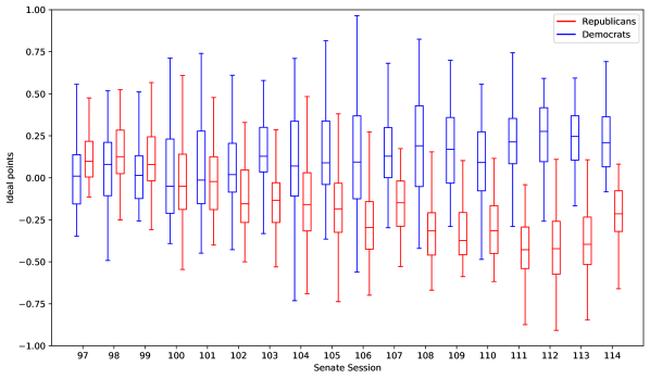
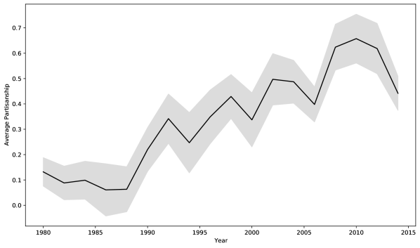
Figure 1: Party- and session-specific ideal point distributions represented as box-plots (top). Estimated average partisanship over the years together with approximate pointwise 95% confidence intervals (bottom).

Figure 1 (bottom) depicts the evolvment of these average partisanship estimates over time. The gray shaded area represents the approximate pointwise $95\%$ confidence intervals of the partisanship measure estimate based on the individual estimates. Clearly, before the 1990s, the TV-TBIP model does not detect any noteworthy partisanship in the speeches given in the U.S. Senate. However, at the beginning of the 1990s, the estimated average partisanship between Democrats and Republicans increases rapidly and reaches a maximum around 2010, while it is slightly decreasing afterwards. This pattern of evolvment of partisanship is in line with results obtained using the supervised model proposed in Gentzkow et al. (2019a).

To further validate our aggregate measure of partisanship, we compare it with the scores of the first dimension obtained with the DW-Nominate procedure proposed by McCarty et al. (1997). Based on the first dimension DW-Nominate scores, we estimate the average partisanship as the difference between the average DW-Nominate scores of Republicans and Democrats. We find an average correlation of $0.77$ between both partisanship estimates indicating that our text based average partisanship measure captures the same effect over time as the DW-Nominate scores.

	Min.	1st Qu.	Median	Mean	3rd Qu.	Max.	SD	Sessions (#)
	Most liberal Democrats
Byron Dorgan (D)	0.68	0.73	0.87	0.86	0.98	1.08	0.15	105$-$111 (7)
Dale Bumpers (D)	0.68	0.68	0.68	0.68	0.68	0.68		105$-$105 (1)
Thomas Harkin (D)	0.21	0.48	0.57	0.63	0.66	1.14	0.27	105$-$113 (9)
Christopher Murphy (D)	0.43	0.50	0.56	0.56	0.63	0.69	0.18	113$-$114 (2)
Paul Wellstone (D)	0.41	0.45	0.48	0.53	0.59	0.69	0.15	105$-$107 (3)
	Most conservative Democrats
Daniel Inouye (D)	$-$0.56	$-$0.31	$-$0.13	$-$0.14	0.08	0.20	0.28	105$-$112 (8)
Robert Torricelli (D)	$-$0.27	$-$0.20	$-$0.13	$-$0.16	$-$0.10	$-$0.06	0.11	105$-$107 (3)
Ben Nelson (D)	$-$0.26	$-$0.24	$-$0.19	$-$0.17	$-$0.14	$-$0.01	0.09	107$-$112 (6)
Arlen Specter (D)	$-$0.29	$-$0.27	$-$0.24	$-$0.18	$-$0.12	0.00	0.16	109$-$111 (3)
Evan Bayh (D)	$-$1.14	$-$1.07	$-$0.52	$-$0.49	0.06	0.22	0.65	106$-$111 (6)
	Most conservative Republicans
Jesse Helms (R)	$-$1.42	$-$1.28	$-$1.15	$-$1.14	$-$1.01	$-$0.86	0.28	105$-$107 (3)
Gordon Smith (R)	$-$1.49	$-$1.34	$-$0.77	$-$0.80	$-$0.27	$-$0.14	0.61	105$-$110 (6)
John Barrasso (R)	$-$0.94	$-$0.89	$-$0.67	$-$0.71	$-$0.57	$-$0.47	0.20	110$-$114 (5)
John Hoeven (R)	$-$0.91	$-$0.77	$-$0.62	$-$0.69	$-$0.59	$-$0.55	0.19	112$-$114 (3)
Mike Johanns (R)	$-$0.61	$-$0.60	$-$0.59	$-$0.59	$-$0.57	$-$0.56	0.03	111$-$113 (3)
	Most liberal Republicans
Ed Bryant (R)	0.01	0.01	0.01	0.01	0.01	0.01		106$-$106 (1)
John Chafee (R)	0.09	0.09	0.09	0.09	0.09	0.09		105$-$105 (1)
Dirk Kempthorne (R)	0.14	0.14	0.14	0.14	0.14	0.14		105$-$105 (1)
Phil Gramm (R)	0.06	0.12	0.18	0.16	0.22	0.25	0.10	105$-$107 (3)
Howard McKeon (R)	0.21	0.21	0.21	0.21	0.21	0.21		111$-$111 (1)
	Independent Senators
James Jeffords (I)	$-$0.16	$-$0.16	$-$0.15	$-$0.15	$-$0.14	$-$0.14	0.01	107$-$109 (3)
Bernard Sanders (I)	0.50	0.62	0.68	0.71	0.86	0.88	0.16	110$-$114 (5)
Joseph Lieberman (I)	$-$0.02	0.01	0.05	0.05	0.08	0.12	0.07	110$-$112 (3)
Angus King (I)	0.09	0.09	0.10	0.10	0.11	0.11	0.02	113$-$114 (2)

Table 1: Overview on the estimated ideal points for the last ten Congress sessions, i.e., starting with session 105, for selected Democrat and Republican speakers. The five most liberal and conservative speakers for each party according to their average ideal point values are included as well as the independent speakers. The estimated ideal points are summarized using the five-point summary (minimum – Min.; 1st quartile – 1st Qu.; Median; Mean; 3rd quartile – 3rd Qu.; maximum - Max.; standard deviation – SD). The specific sessions (Sessions) when the speaker was a member of the Senate during these last ten Congress sessions are also given together with the number of sessions in parentheses (#).

Table 1 displays the estimated ideological positions of selected Republican and Democrat speakers for the last 10 sessions, i.e., we consider results from session 105 onwards. For Republicans as well as Democrats, we display the five most liberal and conservative speakers according to their mean ideal point over the last 10 sessions per party. Table 1 indicates that according to TV-TBIP, the most liberal Democrats are Byron Dorgan, Dale Bumpers, Thomas Harkin, Christopher Murphy and Paul Wellstone. Dorgan served 12 years in the U.S. House and 18 years in the Senate (here we consider the seven sessions 105 to 111). According to his speeches given in the Senate, he is ranked as the most liberal Senator in the considered period. This seems to be surprising at first glance, in particular because his DW-Nominate score of $-0.267$ only puts him in the middle of the political spectrum of Democrats based on voting decisions. However, as a Chairman of the Senate Energy Panel, he was an early supporter of renewable energy, e.g., sponsoring measures on the production tax credit for wind energy. We also find Paul Wellston among the top five most liberal Democratic Senators. This is completely in line with the DW-Nominate scores. According to these voting-based scores, he is the most liberal Democratic Senator during sessions 105–107. Analyzing the conservative spectrum of Democratic Senators in the Senate, we find that Evan Bayh is most conservative. This is again in line with the DW-Nominate score, where he is ranked the third most conservative Democrat of session 106. Evan Bayh has a mixed but left-leaning record on civil-rights and was called a “fence-sitter” on climate change which might be caused by the fact that his home state is heavily dependent on coal. Further we find Arlen Specter in the list. He was a Democrat from 1951 to 1965, then a Republican between 1965 and 2009, before switching back to the Democratic Party in 2009. According to TV-TBIP, he is classified as the second most conservative Democrat Senator. The DW-Nominate score for session 111 categorizes him as the most liberal Republican.

Proceeding with the Republican Party, we find Jesse Helms, a Senator from North Carolina, to be the most conservative Republican. The New York Times (see Holmes, 2008) stated that Helms was “bitterly opposed” to federal financing for research and treatment of AIDS which he believed was God’s punishment for homosexuals (see, e.g., Noden, 2007). According to the DW-Nominate score, Jesse Helms is also ranked as the most conservative Republican for, e.g., sessions 106 and 107. The second ranked among the most conservative Republicans is Gordon Smith. “Smith is often described as politically moderate, but has strong conservative credentials as well” (see Wikipedia, 2022b). According to TV-TBIP, he is second ranked among the Republicans based on the mean ideal point value. In addition a high standard deviation of his ideal points over time is observed and the maximum ideal point value estimated for Gordon Smith is $-0.14$. With such an ideal point value he would rather be considered a moderate Republican. Further research might focus on the influence of his religious beliefs on the ideal points inferred. Further we also find John Barasso in the list of the most conservative Republicans. Using the DW-Nominate score, he is more conservative than $71\%$ of the Republicans in session 113.

On the liberal side of the Republicans, TV-TBIP places the Californian House Representative Howard McKeon, and Senators Phil Gramm, Dirk Kempthorne, John Chafee and Ed Bryant. John Chafee is among the most liberal Republicans according to the DW-Nominate score which rates him as being more liberal than $96\%$ of Republicans in session 105. Interestingly, the five Republicans which are characterized as being most liberal by the TV-TBIP model, only serve for a single session in Senate. A similar pattern is not discernible for the five most conservative Republicans or the Democrats identified as being most liberal or conservative according to their average ideal point estimate. Additional research seems to be warranted to investigate if indeed liberal Republicans are at risk to serve only for a short time in the Senate.

Finally, for the speakers who are categorized as independent, the pattern of ideal points estimated is rather evident. Bernie Sanders is the most liberal one, also in the Democratic party he would be ranked second. On the other hand, former Democrat Joe Liebermann is categorized as having a slightly liberal position and former Republican Jim Jeffords seems to have a tendency to be on the conservative side.

3.3 Topics

An advantage of the TV-TBIP model compared to the text based partisanship model proposed by Gentzkow et al. (2019b) is that our model does not only estimate the topics in a data-driven way but also allows the term compositions to change over time to account for newly emerging or subduing sub-themes within a topic. This enables interpretation and inspection of the evolvment of topics over time. In addition to time having an influence on term prevalence in topics, also the latent dimension induces different term prevalences in topics in dependence of the position of the speaker in the latent dimension. This influence of polarity might also vary across topics.

	Session 97 (from January 3, 1981, to January 3, 1983)	Session 114 (from January 3, 2015, to January 3, 2017)
T1	$\underset{(0.315)}{\textrm{united states}}$, $\underset{(0.008)}{\textrm{foreign policy}}$, $\underset{(0.007)}{\textrm{international trade}}$, $\underset{(0.006)}{\textrm{foreign relations}}$, $\underset{(0.005)}{\textrm{acid rain}}$	$\underset{(0.389)}{\textrm{united states}}$, $\underset{(0.022)}{\textrm{puerto rico}}$, $\underset{(0.021)}{\textrm{trade agreements}}$, $\underset{(0.014)}{\textrm{trade promotion}}$, $\underset{(0.013)}{\textrm{promotion authority}}$
T2	$\underset{(0.03)}{\textrm{private sector}}$, $\underset{(0.021)}{\textrm{small businesses}}$, $\underset{(0.019)}{\textrm{tax credit}}$, $\underset{(0.016)}{\textrm{internal revenue}}$, $\underset{(0.011)}{\textrm{clean air}}$	$\underset{(0.049)}{\textrm{small businesses}}$, $\underset{(0.026)}{\textrm{american workers}}$, $\underset{(0.025)}{\textrm{exportimport bank}}$, $\underset{(0.02)}{\textrm{exim bank}}$, $\underset{(0.019)}{\textrm{economic growth}}$
T3	$\underset{(0.071)}{\textrm{legal services}}$, $\underset{(0.032)}{\textrm{services corporation}}$, $\underset{(0.007)}{\textrm{legal assistance}}$, $\underset{(0.007)}{\textrm{older americans}}$, $\underset{(0.006)}{\textrm{human resources}}$	$\underset{(0.024)}{\textrm{medical research}}$, $\underset{(0.02)}{\textrm{state university}}$, $\underset{(0.018)}{\textrm{high school}}$, $\underset{(0.018)}{\textrm{passed away}}$, $\underset{(0.013)}{\textrm{national institutes}}$
T4	$\underset{(0.095)}{\textrm{supreme court}}$, $\underset{(0.03)}{\textrm{federal courts}}$, $\underset{(0.015)}{\textrm{public schools}}$, $\underset{(0.015)}{\textrm{federal court}}$, $\underset{(0.014)}{\textrm{school prayer}}$	$\underset{(0.146)}{\textrm{supreme court}}$, $\underset{(0.03)}{\textrm{attorney general}}$, $\underset{(0.017)}{\textrm{justice scalia}}$, $\underset{(0.015)}{\textrm{district court}}$, $\underset{(0.013)}{\textrm{judicial nominees}}$
T5	$\underset{(0.13)}{\textrm{interest rates}}$, $\underset{(0.048)}{\textrm{high interest}}$, $\underset{(0.035)}{\textrm{federal reserve}}$, $\underset{(0.021)}{\textrm{interest rate}}$, $\underset{(0.016)}{\textrm{reserve board}}$	$\underset{(0.061)}{\textrm{wall street}}$, $\underset{(0.02)}{\textrm{federal reserve}}$, $\underset{(0.012)}{\textrm{protection act}}$, $\underset{(0.011)}{\textrm{financial crisis}}$, $\underset{(0.008)}{\textrm{monetary policy}}$
T6	$\underset{(0.077)}{\textrm{natural gas}}$, $\underset{(0.015)}{\textrm{energy assistance}}$, $\underset{(0.011)}{\textrm{gas prices}}$, $\underset{(0.01)}{\textrm{policy act}}$, $\underset{(0.008)}{\textrm{lowincome energy}}$	$\underset{(0.086)}{\textrm{home state}}$, $\underset{(0.021)}{\textrm{important issue}}$, $\underset{(0.016)}{\textrm{critically important}}$, $\underset{(0.012)}{\textrm{transportation system}}$, $\underset{(0.01)}{\textrm{surface transportation}}$
T7	$\underset{(0.045)}{\textrm{law enforcement}}$, $\underset{(0.018)}{\textrm{criminal justice}}$, $\underset{(0.018)}{\textrm{violent crime}}$, $\underset{(0.017)}{\textrm{coast guard}}$, $\underset{(0.014)}{\textrm{attorney general}}$	$\underset{(0.082)}{\textrm{law enforcement}}$, $\underset{(0.026)}{\textrm{human trafficking}}$, $\underset{(0.021)}{\textrm{mental health}}$, $\underset{(0.014)}{\textrm{gun violence}}$, $\underset{(0.013)}{\textrm{criminal justice}}$
T8	$\underset{(0.078)}{\textrm{saudi arabia}}$, $\underset{(0.068)}{\textrm{middle east}}$, $\underset{(0.026)}{\textrm{foreign policy}}$, $\underset{(0.018)}{\textrm{persian gulf}}$, $\underset{(0.015)}{\textrm{foreign relations}}$	$\underset{(0.143)}{\textrm{national security}}$, $\underset{(0.034)}{\textrm{middle east}}$, $\underset{(0.03)}{\textrm{united states}}$, $\underset{(0.016)}{\textrm{al qaeda}}$, $\underset{(0.013)}{\textrm{islamic state}}$
T9	$\underset{(0.071)}{\textrm{balanced budget}}$, $\underset{(0.032)}{\textrm{federal budget}}$, $\underset{(0.029)}{\textrm{federal spending}}$, $\underset{(0.022)}{\textrm{budget process}}$, $\underset{(0.017)}{\textrm{debt limit}}$	$\underset{(0.019)}{\textrm{appropriations process}}$, $\underset{(0.018)}{\textrm{balanced budget}}$, $\underset{(0.017)}{\textrm{control act}}$, $\underset{(0.014)}{\textrm{budget act}}$, $\underset{(0.013)}{\textrm{budget control}}$
T10	$\underset{(0.033)}{\textrm{budget authority}}$, $\underset{(0.016)}{\textrm{budget act}}$, $\underset{(0.011)}{\textrm{supplemental appropriations}}$, $\underset{(0.01)}{\textrm{block grant}}$, $\underset{(0.01)}{\textrm{loan program}}$	$\underset{(0.057)}{\textrm{high school}}$, $\underset{(0.03)}{\textrm{left behind}}$, $\underset{(0.025)}{\textrm{child left}}$, $\underset{(0.023)}{\textrm{higher education}}$, $\underset{(0.015)}{\textrm{school districts}}$
T11	$\underset{(0.045)}{\textrm{nuclear waste}}$, $\underset{(0.024)}{\textrm{spent fuel}}$, $\underset{(0.022)}{\textrm{nuclear power}}$, $\underset{(0.018)}{\textrm{clinch river}}$, $\underset{(0.015)}{\textrm{public health}}$	$\underset{(0.074)}{\textrm{climate change}}$, $\underset{(0.045)}{\textrm{public health}}$, $\underset{(0.03)}{\textrm{clean water}}$, $\underset{(0.021)}{\textrm{zika virus}}$, $\underset{(0.016)}{\textrm{fossil fuel}}$
T12	$\underset{(0.061)}{\textrm{tax cut}}$, $\underset{(0.029)}{\textrm{tax cuts}}$, $\underset{(0.015)}{\textrm{tax increase}}$, $\underset{(0.014)}{\textrm{economic recovery}}$, $\underset{(0.013)}{\textrm{tax rates}}$	$\underset{(0.057)}{\textrm{middle class}}$, $\underset{(0.028)}{\textrm{tax credit}}$, $\underset{(0.025)}{\textrm{tax code}}$, $\underset{(0.02)}{\textrm{republican budget}}$, $\underset{(0.018)}{\textrm{tax reform}}$
T13	$\underset{(0.06)}{\textrm{voting rights}}$, $\underset{(0.048)}{\textrm{rights act}}$, $\underset{(0.036)}{\textrm{civil rights}}$, $\underset{(0.02)}{\textrm{justice department}}$, $\underset{(0.015)}{\textrm{attorney general}}$	$\underset{(0.046)}{\textrm{civil rights}}$, $\underset{(0.022)}{\textrm{voting rights}}$, $\underset{(0.021)}{\textrm{equal pay}}$, $\underset{(0.018)}{\textrm{rights act}}$, $\underset{(0.014)}{\textrm{fair housing}}$
T14	$\underset{(0.109)}{\textrm{federal government}}$, $\underset{(0.022)}{\textrm{local governments}}$, $\underset{(0.009)}{\textrm{public law}}$, $\underset{(0.009)}{\textrm{federal funds}}$, $\underset{(0.008)}{\textrm{federal agencies}}$	$\underset{(0.157)}{\textrm{federal government}}$, $\underset{(0.037)}{\textrm{private sector}}$, $\underset{(0.026)}{\textrm{taxpayer dollars}}$, $\underset{(0.02)}{\textrm{federal agencies}}$, $\underset{(0.015)}{\textrm{local governments}}$
T15	$\underset{(0.057)}{\textrm{health care}}$, $\underset{(0.016)}{\textrm{veterans administration}}$, $\underset{(0.015)}{\textrm{older americans}}$, $\underset{(0.014)}{\textrm{medical care}}$, $\underset{(0.011)}{\textrm{senior citizens}}$	$\underset{(0.161)}{\textrm{health care}}$, $\underset{(0.04)}{\textrm{affordable care}}$, $\underset{(0.039)}{\textrm{care act}}$, $\underset{(0.038)}{\textrm{health insurance}}$, $\underset{(0.038)}{\textrm{planned parenthood}}$
T16	$\underset{(0.081)}{\textrm{peace corps}}$, $\underset{(0.022)}{\textrm{foreign relations}}$, $\underset{(0.009)}{\textrm{distinguished colleague}}$, $\underset{(0.008)}{\textrm{intelligence activities}}$, $\underset{(0.005)}{\textrm{equally divided}}$	$\underset{(0.046)}{\textrm{next week}}$, $\underset{(0.045)}{\textrm{equally divided}}$, $\underset{(0.035)}{\textrm{en bloc}}$, $\underset{(0.025)}{\textrm{important legislation}}$, $\underset{(0.017)}{\textrm{final passage}}$
T17	$\underset{(0.136)}{\textrm{soviet union}}$, $\underset{(0.026)}{\textrm{world war}}$, $\underset{(0.02)}{\textrm{foreign policy}}$, $\underset{(0.018)}{\textrm{war ii}}$, $\underset{(0.013)}{\textrm{chemical weapons}}$	$\underset{(0.061)}{\textrm{world war}}$, $\underset{(0.051)}{\textrm{war ii}}$, $\underset{(0.045)}{\textrm{puerto rico}}$, $\underset{(0.014)}{\textrm{vietnam war}}$, $\underset{(0.013)}{\textrm{loved ones}}$
T18	$\underset{(0.048)}{\textrm{nuclear weapons}}$, $\underset{(0.045)}{\textrm{arms control}}$, $\underset{(0.025)}{\textrm{nuclear war}}$, $\underset{(0.022)}{\textrm{foreign relations}}$, $\underset{(0.016)}{\textrm{nuclear arms}}$	$\underset{(0.037)}{\textrm{united states}}$, $\underset{(0.035)}{\textrm{nuclear weapons}}$, $\underset{(0.031)}{\textrm{nuclear weapon}}$, $\underset{(0.026)}{\textrm{nuclear program}}$, $\underset{(0.02)}{\textrm{middle east}}$
T19	$\underset{(0.22)}{\textrm{social security}}$, $\underset{(0.028)}{\textrm{security system}}$, $\underset{(0.02)}{\textrm{minimum benefit}}$, $\underset{(0.02)}{\textrm{trust fund}}$, $\underset{(0.018)}{\textrm{security benefits}}$	$\underset{(0.142)}{\textrm{social security}}$, $\underset{(0.056)}{\textrm{trust fund}}$, $\underset{(0.023)}{\textrm{highway trust}}$, $\underset{(0.011)}{\textrm{older americans}}$, $\underset{(0.011)}{\textrm{security administration}}$
T20	$\underset{(0.059)}{\textrm{armed services}}$, $\underset{(0.05)}{\textrm{air force}}$, $\underset{(0.022)}{\textrm{armed forces}}$, $\underset{(0.02)}{\textrm{basing mode}}$, $\underset{(0.017)}{\textrm{national guard}}$	$\underset{(0.051)}{\textrm{air force}}$, $\underset{(0.048)}{\textrm{armed services}}$, $\underset{(0.045)}{\textrm{defense authorization}}$, $\underset{(0.042)}{\textrm{national defense}}$, $\underset{(0.023)}{\textrm{national guard}}$
T21	$\underset{(0.025)}{\textrm{oil companies}}$, $\underset{(0.022)}{\textrm{natural resources}}$, $\underset{(0.017)}{\textrm{windfall profit}}$, $\underset{(0.017)}{\textrm{crude oil}}$, $\underset{(0.016)}{\textrm{profit tax}}$	$\underset{(0.021)}{\textrm{natural resources}}$, $\underset{(0.02)}{\textrm{keystone xl}}$, $\underset{(0.019)}{\textrm{natural gas}}$, $\underset{(0.017)}{\textrm{energy efficiency}}$, $\underset{(0.017)}{\textrm{water conservation}}$
T22	$\underset{(0.08)}{\textrm{human rights}}$, $\underset{(0.03)}{\textrm{united nations}}$, $\underset{(0.027)}{\textrm{genocide convention}}$, $\underset{(0.02)}{\textrm{foreign relations}}$, $\underset{(0.019)}{\textrm{state department}}$	$\underset{(0.056)}{\textrm{human rights}}$, $\underset{(0.041)}{\textrm{state department}}$, $\underset{(0.032)}{\textrm{foreign relations}}$, $\underset{(0.023)}{\textrm{religious freedom}}$, $\underset{(0.019)}{\textrm{united nations}}$
T23	$\underset{(0.051)}{\textrm{national security}}$, $\underset{(0.033)}{\textrm{inspector general}}$, $\underset{(0.023)}{\textrm{defense department}}$, $\underset{(0.021)}{\textrm{national defense}}$, $\underset{(0.014)}{\textrm{defense spending}}$	$\underset{(0.108)}{\textrm{homeland security}}$, $\underset{(0.034)}{\textrm{cyber security}}$, $\underset{(0.017)}{\textrm{usa freedom}}$, $\underset{(0.017)}{\textrm{freedom act}}$, $\underset{(0.015)}{\textrm{inspector general}}$
T24	$\underset{(0.04)}{\textrm{food stamp}}$, $\underset{(0.021)}{\textrm{school lunch}}$, $\underset{(0.02)}{\textrm{food stamps}}$, $\underset{(0.019)}{\textrm{puerto rico}}$, $\underset{(0.019)}{\textrm{stamp program}}$	$\underset{(0.016)}{\textrm{economic development}}$, $\underset{(0.014)}{\textrm{local communities}}$, $\underset{(0.014)}{\textrm{puerto rico}}$, $\underset{(0.011)}{\textrm{foster care}}$, $\underset{(0.01)}{\textrm{much needed}}$
T25	$\underset{(0.041)}{\textrm{executive branch}}$, $\underset{(0.032)}{\textrm{legislative veto}}$, $\underset{(0.024)}{\textrm{regulatory reform}}$, $\underset{(0.018)}{\textrm{federal trade}}$, $\underset{(0.017)}{\textrm{trade commission}}$	$\underset{(0.018)}{\textrm{bipartisan basis}}$, $\underset{(0.014)}{\textrm{good friend}}$, $\underset{(0.011)}{\textrm{bipartisan way}}$, $\underset{(0.011)}{\textrm{democratic colleagues}}$, $\underset{(0.011)}{\textrm{ common ground}}$

Table 2: Most frequent terms for each topic for session 97 (left) and session 114 (right). Values in parenthesis denote appearance rates.

We estimated 25 topics which is in line with Gentzkow et al. (2019b) who used 22 predefined manually coded topics. Table 2 displays the five most frequent terms of the neutral topics for the first and the last session considered. Values in parenthesis denote the proportions of these terms within the topic, i.e., they are determined by normalizing the term-specific Poisson rates $\bm{\beta}$ to sum to one. Inspecting the bigrams listed with their prevalence rates allows to interpret the topics and infer what their content is.

Table 2 indicates that the first topic is mainly concerned with the United States. This bigram has by far the highest appearance rate (approximately $0.3$ for both sessions) across all bigrams in the vocabulary. This appearance rate is also extremely high compared to the appearance rates of any other bigram for all other topics. The additional bigrams listed as having the highest appearance rates for Topic 1 indicate that this topic is about the United States and their concerns with other states such as international trade, foreign relations, trade agreements. Topic 2 is an economic topic about small businesses and export/import; Topic 3 is about education while Topic 4 is about legal issues with the content focus changing over time from school prayers (session 94) to attorney general (session 114). Selectively characterizing the remaining topics, one can discern that Topic 8 which is about foreign policies in the Middle East and the most frequent terms changed from, e.g., saudi arabia, foreign policy to al quaeda, islamic state. Topic 11 seems to be an environmental/public health topic, where nuclear waste is a prevalent term in session 97, while this is climate change in session 114. Topic 12 is about taxes in general, but moves from a discussion on tax cuts to focus more on taxation and the middle class from the first to the last session.

Given that topic compositions may evolve over time, it is of interest to identify topics which remain rather stable over time in their term composition and topics which are rather volatile. To assess stability of topic composition, we determine the cosine similarity between the estimated term intensities of the same topic for two consecutive sessions. Figure 2 displays a heat map of these cosine similarities. The topics are sorted by their mean cosine similarity with the most stable one being on the top and the most volatile one at the bottom. For this comparison, the term intensities of the neutral topics were used. On the top, we find Topic 1 (the United States topic) which is the most stable topic over time. On the other end of the spectrum, Topic 3 is the most volatile topic in terms of term composition. Table 2 reveals that for this topic the most frequent terms changed from legal terms in the first session analyzed to terms related to education in the last session.

Figure 2 also indicates that the largest change in term composition of topics occurs for Topic 23 from session 112 to 113 with still quite a substantial change in term composition to the subsequent session 114. Inspecting the most frequent terms for Topic 23 for sessions 112 and 113 indicates that the term national security is substituted by homeland security and even more important immigration issues started to be also raised in that topic. Another topic with high volatility in the term composition is Topic 11, the climate change/public health topic. It changed from the discussion of nuclear waste to climate change and public health related issues. Figure 3 displays this evolvment of that topic using word clouds.

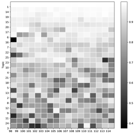
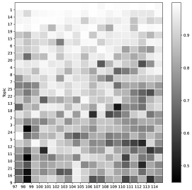
Figure 2: Left: Similarity of the topics for consecutive sessions based on the term compositions of the neutral topics. Right: Similarities between the term compositions of the positive and negative ideological topics for each session.

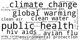
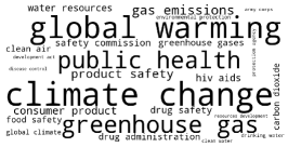
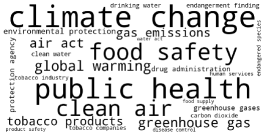
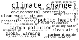
Figure 3: Term prevalences of Topic 11, the public health/climate change topic, across sessions 97 to 114, starting with session 97 on the top left and proceeding row-wise.

In the TV-TBIP model, the term distributions of the topics are also influenced by the polarity scores of the speakers. This means that liberal speakers use different terms than conservative ones even when they are talking about the same topic. To analyze this we inspect the term compositions of the topics for a liberal speaker with ideal point value $1$ and a conservative one with ideal point value $-1$. Table 3 displays the most frequent terms per topic for speakers with a liberal and a conservative position for session 114. We restrict this analysis to a session at the end of the observation period as in this session the latent dimension clearly allowed to discriminate between Republican and Democrat speakers.

	Most frequent positive terms	Most frequent negative terms
T- 1	$\underset{(0.416)}{\textrm{united states}}$, $\underset{(0.04)}{\textrm{puerto rico}}$, $\underset{(0.01)}{\textrm{trade agreements}}$, $\underset{(0.009)}{\textrm{transpacific partnership}}$, $\underset{(0.007)}{\textrm{trade promotion}}$	$\underset{(0.277)}{\textrm{united states}}$, $\underset{(0.034)}{\textrm{trade agreements}}$, $\underset{(0.021)}{\textrm{promotion authority}}$, $\underset{(0.021)}{\textrm{trade promotion}}$, $\underset{(0.015)}{\textrm{currency manipulation}}$
T- 2	$\underset{(0.035)}{\textrm{exportimport bank}}$, $\underset{(0.03)}{\textrm{small businesses}}$, $\underset{(0.029)}{\textrm{american workers}}$, $\underset{(0.029)}{\textrm{minimum wage}}$, $\underset{(0.026)}{\textrm{exim bank}}$	$\underset{(0.055)}{\textrm{small businesses}}$, $\underset{(0.026)}{\textrm{economic growth}}$, $\underset{(0.017)}{\textrm{american workers}}$, $\underset{(0.013)}{\textrm{exportimport bank}}$, $\underset{(0.011)}{\textrm{labor relations}}$
T- 3	$\underset{(0.039)}{\textrm{medical research}}$, $\underset{(0.019)}{\textrm{national institutes}}$, $\underset{(0.017)}{\textrm{state university}}$, $\underset{(0.015)}{\textrm{passed away}}$, $\underset{(0.013)}{\textrm{high school}}$	$\underset{(0.019)}{\textrm{high school}}$, $\underset{(0.018)}{\textrm{pay tribute}}$, $\underset{(0.017)}{\textrm{state university}}$, $\underset{(0.016)}{\textrm{passed away}}$, $\underset{(0.012)}{\textrm{public servant}}$
T- 4	$\underset{(0.122)}{\textrm{supreme court}}$, $\underset{(0.034)}{\textrm{attorney general}}$, $\underset{(0.016)}{\textrm{district court}}$, $\underset{(0.015)}{\textrm{court nominee}}$, $\underset{(0.015)}{\textrm{judge garland}}$	$\underset{(0.13)}{\textrm{supreme court}}$, $\underset{(0.028)}{\textrm{justice scalia}}$, $\underset{(0.021)}{\textrm{attorney general}}$, $\underset{(0.016)}{\textrm{presidential election}}$, $\underset{(0.011)}{\textrm{confirmation process}}$
T- 5	$\underset{(0.085)}{\textrm{wall street}}$, $\underset{(0.015)}{\textrm{federal reserve}}$, $\underset{(0.012)}{\textrm{financial crisis}}$, $\underset{(0.009)}{\textrm{financial institutions}}$, $\underset{(0.008)}{\textrm{consumer protection}}$	$\underset{(0.029)}{\textrm{wall street}}$, $\underset{(0.018)}{\textrm{federal reserve}}$, $\underset{(0.016)}{\textrm{protection act}}$, $\underset{(0.012)}{\textrm{banking housing}}$, $\underset{(0.01)}{\textrm{monetary policy}}$
T- 6	$\underset{(0.075)}{\textrm{home state}}$, $\underset{(0.015)}{\textrm{important issue}}$, $\underset{(0.015)}{\textrm{critically important}}$, $\underset{(0.013)}{\textrm{transportation system}}$, $\underset{(0.011)}{\textrm{roads highways}}$	$\underset{(0.073)}{\textrm{home state}}$, $\underset{(0.023)}{\textrm{important issue}}$, $\underset{(0.014)}{\textrm{critically important}}$, $\underset{(0.011)}{\textrm{faa reauthorization}}$, $\underset{(0.009)}{\textrm{bottom line}}$
T- 7	$\underset{(0.067)}{\textrm{law enforcement}}$, $\underset{(0.024)}{\textrm{gun violence}}$, $\underset{(0.022)}{\textrm{background checks}}$, $\underset{(0.021)}{\textrm{mental health}}$, $\underset{(0.021)}{\textrm{background check}}$	$\underset{(0.078)}{\textrm{law enforcement}}$, $\underset{(0.035)}{\textrm{human trafficking}}$, $\underset{(0.017)}{\textrm{mental health}}$, $\underset{(0.016)}{\textrm{criminal justice}}$, $\underset{(0.012)}{\textrm{sex trafficking}}$
T- 8	$\underset{(0.139)}{\textrm{national security}}$, $\underset{(0.028)}{\textrm{middle east}}$, $\underset{(0.023)}{\textrm{united states}}$, $\underset{(0.013)}{\textrm{al qaeda}}$, $\underset{(0.01)}{\textrm{civil war}}$	$\underset{(0.113)}{\textrm{national security}}$, $\underset{(0.034)}{\textrm{united states}}$, $\underset{(0.033)}{\textrm{middle east}}$, $\underset{(0.018)}{\textrm{islamic state}}$, $\underset{(0.016)}{\textrm{al qaeda}}$
T- 9	$\underset{(0.02)}{\textrm{government shutdown}}$, $\underset{(0.02)}{\textrm{control act}}$, $\underset{(0.015)}{\textrm{appropriations process}}$, $\underset{(0.014)}{\textrm{budget deal}}$, $\underset{(0.012)}{\textrm{budget caps}}$	$\underset{(0.029)}{\textrm{balanced budget}}$, $\underset{(0.022)}{\textrm{national debt}}$, $\underset{(0.017)}{\textrm{appropriations process}}$, $\underset{(0.014)}{\textrm{budget act}}$, $\underset{(0.011)}{\textrm{control act}}$
T- 10	$\underset{(0.058)}{\textrm{high school}}$, $\underset{(0.024)}{\textrm{left behind}}$, $\underset{(0.022)}{\textrm{higher education}}$, $\underset{(0.02)}{\textrm{child left}}$, $\underset{(0.018)}{\textrm{student loan}}$	$\underset{(0.044)}{\textrm{high school}}$, $\underset{(0.029)}{\textrm{left behind}}$, $\underset{(0.024)}{\textrm{child left}}$, $\underset{(0.019)}{\textrm{health education}}$, $\underset{(0.019)}{\textrm{education labor}}$
T- 11	$\underset{(0.117)}{\textrm{climate change}}$, $\underset{(0.031)}{\textrm{public health}}$, $\underset{(0.029)}{\textrm{fossil fuel}}$, $\underset{(0.023)}{\textrm{carbon pollution}}$, $\underset{(0.018)}{\textrm{global warming}}$	$\underset{(0.044)}{\textrm{public health}}$, $\underset{(0.044)}{\textrm{clean water}}$, $\underset{(0.034)}{\textrm{climate change}}$, $\underset{(0.024)}{\textrm{zika virus}}$, $\underset{(0.022)}{\textrm{water act}}$
T- 12	$\underset{(0.062)}{\textrm{middle class}}$, $\underset{(0.034)}{\textrm{republican budget}}$, $\underset{(0.023)}{\textrm{tax credit}}$, $\underset{(0.021)}{\textrm{tax breaks}}$, $\underset{(0.012)}{\textrm{tax code}}$	$\underset{(0.036)}{\textrm{tax code}}$, $\underset{(0.035)}{\textrm{middle class}}$, $\underset{(0.03)}{\textrm{tax reform}}$, $\underset{(0.024)}{\textrm{tax credit}}$, $\underset{(0.01)}{\textrm{income tax}}$
T- 13	$\underset{(0.04)}{\textrm{civil rights}}$, $\underset{(0.027)}{\textrm{voting rights}}$, $\underset{(0.022)}{\textrm{rights act}}$, $\underset{(0.02)}{\textrm{citizens united}}$, $\underset{(0.019)}{\textrm{equal pay}}$	$\underset{(0.037)}{\textrm{civil rights}}$, $\underset{(0.017)}{\textrm{equal pay}}$, $\underset{(0.014)}{\textrm{fair housing}}$, $\underset{(0.012)}{\textrm{voting rights}}$, $\underset{(0.011)}{\textrm{rights act}}$
T- 14	$\underset{(0.122)}{\textrm{federal government}}$, $\underset{(0.036)}{\textrm{private sector}}$, $\underset{(0.019)}{\textrm{taxpayer dollars}}$, $\underset{(0.019)}{\textrm{federal agencies}}$, $\underset{(0.012)}{\textrm{local governments}}$	$\underset{(0.146)}{\textrm{federal government}}$, $\underset{(0.028)}{\textrm{private sector}}$, $\underset{(0.026)}{\textrm{taxpayer dollars}}$, $\underset{(0.015)}{\textrm{federal agencies}}$, $\underset{(0.015)}{\textrm{waste fraud}}$
T- 15	$\underset{(0.122)}{\textrm{health care}}$, $\underset{(0.055)}{\textrm{affordable care}}$, $\underset{(0.052)}{\textrm{care act}}$, $\underset{(0.045)}{\textrm{health insurance}}$, $\underset{(0.043)}{\textrm{planned parenthood}}$	$\underset{(0.167)}{\textrm{health care}}$, $\underset{(0.028)}{\textrm{planned parenthood}}$, $\underset{(0.025)}{\textrm{health insurance}}$, $\underset{(0.024)}{\textrm{affordable care}}$, $\underset{(0.023)}{\textrm{care act}}$
T- 16	$\underset{(0.044)}{\textrm{next week}}$, $\underset{(0.02)}{\textrm{equally divided}}$, $\underset{(0.016)}{\textrm{en bloc}}$, $\underset{(0.012)}{\textrm{important legislation}}$, $\underset{(0.012)}{\textrm{final passage}}$	$\underset{(0.062)}{\textrm{equally divided}}$, $\underset{(0.049)}{\textrm{en bloc}}$, $\underset{(0.032)}{\textrm{important legislation}}$, $\underset{(0.029)}{\textrm{next week}}$, $\underset{(0.016)}{\textrm{final passage}}$
T- 17	$\underset{(0.049)}{\textrm{puerto rico}}$, $\underset{(0.047)}{\textrm{world war}}$, $\underset{(0.036)}{\textrm{war ii}}$, $\underset{(0.016)}{\textrm{vietnam war}}$, $\underset{(0.013)}{\textrm{loved ones}}$	$\underset{(0.053)}{\textrm{world war}}$, $\underset{(0.049)}{\textrm{war ii}}$, $\underset{(0.03)}{\textrm{puerto rico}}$, $\underset{(0.017)}{\textrm{choice act}}$, $\underset{(0.013)}{\textrm{veterans administration}}$
T- 18	$\underset{(0.039)}{\textrm{nuclear weapon}}$, $\underset{(0.033)}{\textrm{united states}}$, $\underset{(0.033)}{\textrm{nuclear weapons}}$, $\underset{(0.023)}{\textrm{nuclear program}}$, $\underset{(0.018)}{\textrm{irans nuclear}}$	$\underset{(0.036)}{\textrm{united states}}$, $\underset{(0.03)}{\textrm{nuclear weapons}}$, $\underset{(0.023)}{\textrm{nuclear program}}$, $\underset{(0.02)}{\textrm{middle east}}$, $\underset{(0.02)}{\textrm{nuclear weapon}}$
T- 19	$\underset{(0.115)}{\textrm{social security}}$, $\underset{(0.042)}{\textrm{trust fund}}$, $\underset{(0.022)}{\textrm{highway trust}}$, $\underset{(0.014)}{\textrm{older americans}}$, $\underset{(0.009)}{\textrm{security benefits}}$	$\underset{(0.12)}{\textrm{social security}}$, $\underset{(0.051)}{\textrm{trust fund}}$, $\underset{(0.017)}{\textrm{highway trust}}$, $\underset{(0.012)}{\textrm{security administration}}$, $\underset{(0.009)}{\textrm{disability insurance}}$
T- 20	$\underset{(0.037)}{\textrm{air force}}$, $\underset{(0.036)}{\textrm{defense authorization}}$, $\underset{(0.033)}{\textrm{armed services}}$, $\underset{(0.03)}{\textrm{national defense}}$, $\underset{(0.018)}{\textrm{national guard}}$	$\underset{(0.055)}{\textrm{air force}}$, $\underset{(0.054)}{\textrm{armed services}}$, $\underset{(0.045)}{\textrm{national defense}}$, $\underset{(0.043)}{\textrm{defense authorization}}$, $\underset{(0.024)}{\textrm{national guard}}$
T- 21	$\underset{(0.026)}{\textrm{energy efficiency}}$, $\underset{(0.023)}{\textrm{tar sands}}$, $\underset{(0.022)}{\textrm{water conservation}}$, $\underset{(0.02)}{\textrm{conservation fund}}$, $\underset{(0.018)}{\textrm{clean energy}}$	$\underset{(0.024)}{\textrm{keystone xl}}$, $\underset{(0.021)}{\textrm{natural gas}}$, $\underset{(0.02)}{\textrm{natural resources}}$, $\underset{(0.02)}{\textrm{xl pipeline}}$, $\underset{(0.016)}{\textrm{energy security}}$
T- 22	$\underset{(0.065)}{\textrm{human rights}}$, $\underset{(0.036)}{\textrm{state department}}$, $\underset{(0.028)}{\textrm{foreign relations}}$, $\underset{(0.02)}{\textrm{united nations}}$, $\underset{(0.017)}{\textrm{american citizens}}$	$\underset{(0.047)}{\textrm{religious freedom}}$, $\underset{(0.037)}{\textrm{human rights}}$, $\underset{(0.033)}{\textrm{state department}}$, $\underset{(0.027)}{\textrm{foreign relations}}$, $\underset{(0.022)}{\textrm{religious liberty}}$
T- 23	$\underset{(0.109)}{\textrm{homeland security}}$, $\underset{(0.027)}{\textrm{cyber security}}$, $\underset{(0.019)}{\textrm{usa freedom}}$, $\underset{(0.018)}{\textrm{freedom act}}$, $\underset{(0.018)}{\textrm{immigration reform}}$	$\underset{(0.082)}{\textrm{homeland security}}$, $\underset{(0.034)}{\textrm{cyber security}}$, $\underset{(0.025)}{\textrm{inspector general}}$, $\underset{(0.012)}{\textrm{freedom act}}$, $\underset{(0.012)}{\textrm{usa freedom}}$
T- 24	$\underset{(0.013)}{\textrm{first responders}}$, $\underset{(0.013)}{\textrm{local communities}}$, $\underset{(0.011)}{\textrm{economic development}}$, $\underset{(0.011)}{\textrm{emergency funding}}$, $\underset{(0.009)}{\textrm{grant program}}$	$\underset{(0.019)}{\textrm{puerto rico}}$, $\underset{(0.016)}{\textrm{economic development}}$, $\underset{(0.014)}{\textrm{foster care}}$, $\underset{(0.012)}{\textrm{local communities}}$, $\underset{(0.01)}{\textrm{much needed}}$
T- 25	$\underset{(0.019)}{\textrm{republican colleagues}}$, $\underset{(0.015)}{\textrm{bipartisan basis}}$, $\underset{(0.012)}{\textrm{republican leadership}}$, $\underset{(0.012)}{\textrm{good friend}}$, $\underset{(0.011)}{\textrm{put together}}$	$\underset{(0.018)}{\textrm{democratic colleagues}}$, $\underset{(0.015)}{\textrm{bipartisan basis}}$, $\underset{(0.015)}{\textrm{bipartisan way}}$, $\underset{(0.013)}{\textrm{good friend}}$, $\underset{(0.011)}{\textrm{democratic friends}}$

Table 3: Most frequent positive (left) and negative (right) terms for each topic for session 114. Values in parenthesis denote appearance rates.

Results indicate that for Topic 21 – which is about natural resources and energy – a speaker with a positive, i.e., a liberal, ideal point uses terms like energy efficiency or clean energy when talking about this topic while a conservative one uses terms like keystone xl (a pipeline project by TC Energy) or energy security. For Topic 5, which is about monetary policy, we find on the liberal side terms like financial crisis and consumer protection but on the conservative side banking housing and monetary policy.

We complement this comparison of the term compositions of positive and negative topics for a single session by systematically analyzing how the term distributions for each topic differ as induced by the latent polarity across all sessions. We create again a heat map of the cosine similarity matrix, this time comparing the term frequencies of positive and negative topics for each topic and session. The term prevalences of the positive and negative topics are determined using an ideal point of $1$ (i.e., liberal) and $-1$ (conservative). The results are displayed in Figure 2 on the right. In line with the previous results we find that Topic 1 is the most “neutral”, i.e., the topic where the differences between the terms used by liberal and conservative speakers are smallest. In addition we also observe low discordance for Topic 14 which is about the federal government and Topic 17 which is obviously about war veterans. The climate change/public health Topic 11 is at the bottom of the heat map in Figure 2 on the right, indicating that there is less congruence in the wording of Democrats and Republican when talking about these issues. The same holds for Topic 21, another energy topic which is ranked as the third least congruent topic. Only Topic 9 (which is about government shutdowns and budget control) and Topic 16 (which appears to be a derivation thereof) have a lower concordance.

4 Conclusion and Discussion

In this work we proposed the time varying text based ideal point model (TV-TBIP) and used this model to analyze the speeches delivered between 1981 to 2017 in the U.S. Senate. This model extends the TBIP model proposed by Vafa et al. (2020) and allows for an unsupervised categorization of speeches and speakers over time.

The advantages of our approach compared to other text based partisanship studies put forward in the literature, e.g., by Gentzkow et al. (2019b) are threefold: Firstly, our approach is unsupervised and does not include the party membership of the speakers in the analysis avoiding issues of overfitting when using high-dimensional data. In addition this approach also allows to include speeches given by independent Senators and positions them along the latent space. Secondly, TV-TBIP combines the class of topic models with ideal point models. Thus, researchers do not have to manually specify topics apriori using key terms. Thirdly, our model is able to detect the accordance of political parties on the topic level through the polarity- and topic-specific term distributions.

The results of the TV-TBIP model also complement insights gained from a vote based analysis. The relative positions of the ideal points in the latent space estimated for the Congress members can be compared to the DW-Nominate scores estimated based on their votes. This highlights congruence as well as discrepancy of voting behavior with the speeches given in the Senate. On an aggregate level based on the partisanship measures estimated from the ideal points as well as the DW-Nominate scores, a clear alignment between these measures is discerned, indicating also a similar pattern in changes in partisanship over time.

Additional insights to previous analyses are possible due to the data-driven estimation of the topics. In particular, cosine similarities between topics of subsequent sessions allow to detect which topics evolve more over time than others. We identify the climate change/public health topic as being particularly variable over time and we then highlight the evolvment of the climate change/public health topic over time by visualizing word clouds for each session. A general assessment of how well topics in each session allow to discriminate between the parties is also based on cosine similarity. Again the climate change/public health topic stands out and shows high discordance in term composition across the two parties. In addition also the energy topic allows to discriminate between speakers from the two parties, while the topic on war veterans consists of similar term compositions for Democrats and Republicans.

Other applications of the TBIP model in political science may be envisaged. E.g., one could consider the use of the TBIP model to perform research on political events which are either triggered or reflected in text documents. We also conjecture that these models may be used to empirically learn about ambiguity in political discourse (Tolvanen et al., 2021). Some of these applications might require also statistical modeling extensions or refinements such as combining TV-TBIP with a regression framework. This would allow ideal points to also be driven by external covariates, e.g., future elections, outside jobs, etc.

Appendix A More Details on Specifying and Estimating TV-TBIP

A.1 Prior Specification

The parameters are assumed to be independent and identically distributed with the same prior settings used for each time point, speech, term and topic as well as speaker. The priors for the intensity parameters $\theta_{t,ik}$ and $\beta_{t,kv}$ are assumed to follow independent Gamma distributions with potentially different hyperparameters for $\theta_{t,ik}$ and $\beta_{t,kv}$, but identical Gamma distributions for all sessions $t$, speeches $i$, terms $v$ and topics $k$:

$$\theta_{t,ik} \sim\text{Gamma}(\alpha_{1},\alpha_{2}), \beta_{t,kv} \sim\text{Gamma}(\gamma_{1},\gamma_{2}).$$

Careful selection of the parameters of the Gamma distribution is required in order to induce a suitable sparsity in the topic distributions of the speeches and the term distributions of the topics. Sparsity implies that each speech only consists of a small number of topics and that each topic only is characterized by a few terms with high prevalence values. The choice of these hyperparameters thus impacts on the specific solution obtained. This holds true, in particular, for a setting where the model may be assumed to suffer from identifiability issues and where different parameterizations, i.e., factorizations, might capture the co-occurrence patterns in the observed data similarly well. To facilitate interpretability of the topics obtained, such a sparsity characteristic is desirable.

The parameters $\eta_{t,kv}$ and $x_{t,s}$ can take arbitrary values, negative as well as positive. To reflect this unrestricted support, standard normal distributions are imposed as their priors. This means that for all sessions $t$, terms $v$, topics $k$, and speakers $s$, the parameters are apriori independently distributed with:

$$\eta_{t,kv} \sim\text{Normal}(0,1), x_{t,s} \sim\text{Normal}(0,1).$$

Restricting the mean values to zero implies that an average speaker in the latent dimension is viewed as a neutral speaker and the average intensities as modified by the latent dimension represent the neutral topic intensities. Restricting the scale improves identifiability of the model, as this fixes the possible within-topic variability due to changes in the polarity of the speaker.

A.2 Estimation Based on Variational Inference

We follow Vafa et al. (2020) when specifying the variational family to approximate the posterior. The variational family needs to provide sufficient flexibility in order to closely approximate the posterior. For estimating the TV-TBIP model, a mean-field variational family is used. Let $q_{\bm{\phi}_{t}}(\bm{\theta}_{t},\bm{\beta}_{t},\bm{\eta}_{t},\bm{x}_{t})$ be the variational family, indexed by variational parameters $\bm{\phi}_{t}$. Using a mean-field variational family implies that the variational family factorizes over the latent variables, where $i$ indexes speeches, $k$ indexes topics, and $s$ indexes authors:

$$q_{\bm{\phi}_{t}}(\bm{\theta}_{t},\bm{\beta}_{t},\bm{\eta}_{t},\bm{x}_{t}) =\prod_{i}q(\bm{\theta}_{t,i})\prod_{k}q(\bm{\beta}_{t,k})\prod_{k}q(\bm{\eta}_{t,k})\prod_{s}q(\bm{x}_{t,s}).$$

We use log-normal distributions for the positive variables and Gaussian distributions for the real variables:

$$\bm{\theta}_{t,i} \sim\text{LogNormal}_{K}(\bm{\mu}_{\bm{\theta}_{t,i}},I_{K}\sigma_{\bm{\theta}_{t,i}}^{2}), \bm{\beta}_{t,k} \sim\text{LogNormal}_{V}(\bm{\mu}_{\beta_{t,k}},I_{V}\sigma_{\beta_{t,k}}^{2}),$$

$$\bm{\eta}_{t,k} \sim\text{Normal}_{V}(\bm{\mu}_{\eta_{t,k}},I_{V}\sigma_{\eta_{t,k}}^{2}), x_{t,s} \sim\text{Normal}(\mu_{x_{t,s}},\sigma_{x_{t,s}}^{2}),$$

where $I_{K}$ is the identity matrix of dimension $K$ and $I_{V}$ the identity matrix of dimension $V$.

The complete set of variational parameters is thus given by $\bm{\phi}_{t}=\{\{\mu_{\theta_{t,i}}\}_{i}$, $\{\sigma_{\theta_{t,i}}^{2}\}_{i}$, $\{\mu_{\beta_{t,k}}\}_{k}$, $\{\sigma_{\beta_{t,k}}^{2}\}_{k}$, $\{\mu_{\eta_{t,k}}\}_{k}$, $\{\sigma_{\eta_{t,k}}^{2}\}_{k}$, $\{\mu_{x_{t,s}}\}_{s}$, $\{\sigma_{x_{t,s}}^{2}\}_{s}\}$. These variational parameters are determined by maximizing the ELBO as minimizing the Kullback-Leibler divergence is equivalent to maximizing the Evidence Lower BOund (ELBO):

$$\mathbf{E}_{q_{\bm{\phi}_{t}}}[\log p(\bm{\theta}_{t},\bm{\beta}_{t},\bm{\eta}_{t},\bm{x}_{t})+\log p(\bm{c}_{t}|\bm{\theta}_{t},\bm{\beta}_{t},\bm{\eta}_{t},\bm{x}_{t})-\log q_{\bm{\phi}_{t}}(\bm{\theta}_{t},\bm{\beta}_{t},\bm{\eta}_{t},\bm{x}_{t})].$$

Based on the estimated variational parameters, the model parameters are then obtained as the posterior means induced by the estimated $\bm{\phi}_{t}$ values. The maximization of the ELBO is performed using a general purpose optimizer, where initial values need to be provided. Suitable initial values improve the solution obtained as well as the convergence behavior of the optimizer. More details are given in Vafa et al. (2020).

Appendix B More Details on Data and Analysis

B.1 Data Description and Pre-processing

The Stanford University Social Science Data Collection database (Gentzkow et al., 2018) provides already processed text data from the United States Congressional Record. The speeches given by members of the U.S. Congress have been parsed and are stored as transcripts of the full-text speeches together with some related metadata information such as details about the speaker. We use the “daily edition” of the Senate speeches in the database for our analysis which covers sessions 97 to 114 (1981–2017) and provides data on the speech level.

Following Gentzkow et al. (2019b) and Vafa et al. (2020), a number of pre-processing steps were performed to obtain session-specific document-term matrices with an aligned vocabulary from the files containing the transcripted full text speeches. First, we removed punctuation and numbers, changed the text to lower-case and eliminated stop words. For tokenization, we follow Gentzkow et al. (2019b) and also use bigrams. Gentzkow et al. (2019a) argue that in certain applications such as the analysis of partisan speech, single words are insufficient to capture the patterns of interest. They point out that at least bigrams are required to capture a limited amount of the dependence between words and they also emphasize that bigrams are better able to gather overtones and ideological phrases. In addition, using bigrams instead of single terms helps to improve interpretability of the resulting topics when inspecting the topic-specific term prevalences.

For each session, we considered speeches given by Senators as well as House Representatives. We removed speakers who gave less than 24 speeches in a particular session as well as bigrams which were used by less than 10 speakers in a particular session (cf. Vafa et al., 2020). Finally, speeches resulting in an empty frequency count, i.e., an empty row in the document-term matrix, were omitted from further analysis. The complete vocabulary spanning all the sessions from session 97 to 114 resulting from these pre-processing steps consists of 12,527 unique bigrams.

Prior to these pre-processing steps, the dataset of the Senate speeches contains 1,262,273 speeches given by 1,142 unique speakers. After pre-processing we are left with 614,613 speeches spoken by 355 unique speakers (including Senators and House Representatives) over a period of 18 sessions, i.e., during the years 1981 until 2017. Table 4 displays summary statistics of the original data before pre-processing as well as the data obtained after pre-processing which was then used for estimating the TV-TBIP model.

	Speakers		Speeches		$\varnothing$ Speeches
Session	before	after	before	after	before	after
97	376	118	110980	47088	295.16	399.05
98	347	121	97755	42608	281.71	352.13
99	304	104	107774	49271	354.52	473.76
100	302	105	108618	49707	359.66	473.40
101	366	103	90024	44247	245.97	429.58
102	334	103	82233	42234	246.21	410.04
103	346	103	83742	40957	242.03	397.64
104	244	103	89763	42879	367.88	416.30
105	191	100	66512	33591	348.23	335.91
106	200	101	66855	33833	334.28	334.98
107	212	100	62267	30895	293.71	308.95
108	150	100	65776	33571	438.51	335.71
109	170	101	53404	27842	314.14	275.66
110	151	102	51919	27385	343.83	268.48
111	208	104	37728	20236	181.38	194.58
112	126	100	32924	18421	261.30	184.21
113	114	100	29721	16249	260.71	162.49
114	111	99	24278	13599	218.72	137.36

Table 4: Number of speakers, number of speeches and average number of speeches per speaker for each session before and after pre-processing.

B.2 Model Specification and Estimation

Gentzkow et al. (2019b) manually identified 22 substantive topics based on their knowledge of the database. Aiming for a similar granularity in the topics identified in a data-driven way with the TV-TBIP model, we specified the number of topics to be equal to 25 for each session. We want to emphasize that there is no “true” number of topics (see, e.g., Roberts et al., 2019). Estimating only few topics implies that topical content is very “wide”, while a large number of topics might result in very granular and maybe overlapping topics. Similar to Gentzkow et al. (2019b), we also assume that the number of topics is the same across time. However, we allow the topical content to change over time with the term distributions of the topics being allowed to be session-specific.

To complete the model specification, we also have to fix the parameters of the prior distributions of the topic distributions $\bm{\theta}_{t}$, the term distributions $\bm{\beta}_{t}$ as well as the polarity-term distributions $\bm{\eta}_{t}$ and the ideal points $\bm{x}_{t}$. We use standard normal priors for the normal priors of $\bm{\eta}_{t}$ and the ideal points $\bm{x}_{t}$, as already mentioned before. Both the topic prevalences as well as the topic-specific term prevalences follow apriori Gamma priors. Selecting the parameters of these Gamma priors is crucial to induce sparsity in the topic distributions of the speeches as well as the term distributions of the topics. We follow Vafa et al. (2020) for the parameter settings of these priors: We use the same parameter values for both priors, i.e., $\alpha_{1}=\gamma_{1}$ and $\alpha_{2}=\gamma_{2}$. In addition we use the same parameter values for shape and rate of the Gamma distribution, which implies that the prior mean is equal to 1. The specific values selected for the parameters are $\alpha_{1}=\alpha_{2}=0.3$, i.e., a value smaller than one is used which is crucial for sparsity and which implies a prior variance of 1 / 0.3.

The analysis is performed using Python 3.7 (van Rossum et al., 2011), Tensorflow 1.15 GPU (Abadi et al., 2015) and scikit-learn 1.0.2 (Pedregosa et al., 2011). Running the optimizer with GPU support considerably reduces runtime. For optimizing the ELBO function we make use of the Adam optimizer (Kingma and Ba, 2015) using 300,000 iterations per session. Inspection of the ELBO values indicated convergence after about 100,000 iterations.

Appendix C Additional Results

C.1 Ideal Points of Speakers

The session- and party-specific ideal point distributions estimated by TV-TBIP are analyzed using box-plots in the main paper. An alternative view is provided in Figure 4 where their kernel density estimates are visualized. The density estimates for each of the two parties for the same session are combined in one panel and the sessions are arranged row-wise across time. Kernel density estimates provide a more flexible and detailed view on the distribution of the ideal points compared to the box-plots. The kernel density estimates indicate that the within party- and session-specific ideal point distributions are approximately unimodal and that these modes between the two parties separate over time, reducing also considerably the overlap of the estimated densities.

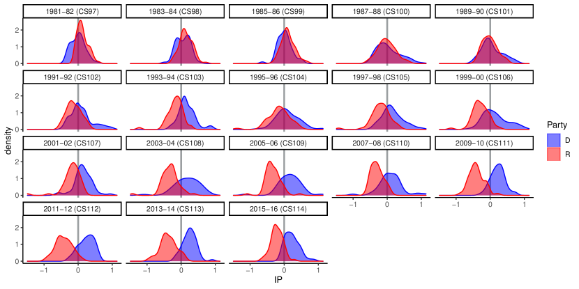
Figure 4: Kernel density plots characterizing session- and party-specific ideal point distributions.

We further investigate the ideal points estimated by the TV-TBIP for the speakers and in particular their evolvment over time by focusing on speakers who were members of the Senate during the whole analysis period and hence have ideal point estimated for each session. Figure 5 displays the development of estimated ideal points of the four speakers who were members of the Senate during the whole analysis period. These speakers are three Republicans and one Democrat, namely Thad Cochran (R), Charles Grassley (R), Patrick Leahy (D) and Orrin Hatch (R). Inspection of the evolvment of the ideal points for those four speakers provides the following interesting insights: Firstly, we can discern a drop in the ideal points of all four Senators after the Contract with America. The reasons are not obvious and one can only speculate. One possible explanation could be the Congress turnover which took place. At this point in time, it was the first time after 40 years that Republicans had the majority in the Congress. Secondly, Figure 5 confirms that the ordering of the ideological positions of TV-TBIP is reasonable. Among these four Senators, the most liberal Senator Patrick Leahy (D) clearly has the highest ideal point values for the latter time periods, while the three Republican Senators are after the Contract with America consistently positioned on the negative side of the ideological scale. Among the three Republicans displayed in Figure 5, we find Thad Cochran to be the most liberal one. Indeed Thad Cochran is usually considered to be more moderate than most of his Republican colleagues (e.g., Enten, 2014). For example, in 2017, the New York Times arranged Republican Senators based on ideology and reported that Thad Cochran was the fourth most moderate Republican (see Parlapiano and Benzaquen, 2017). On the other side of the spectrum we find Orrin Hatch (R), one of the leading figures behind the Senate’s anti-terrorism bill, and a person who is strongly opposed to abortion (see, e.g., Wikipedia, 2022c).

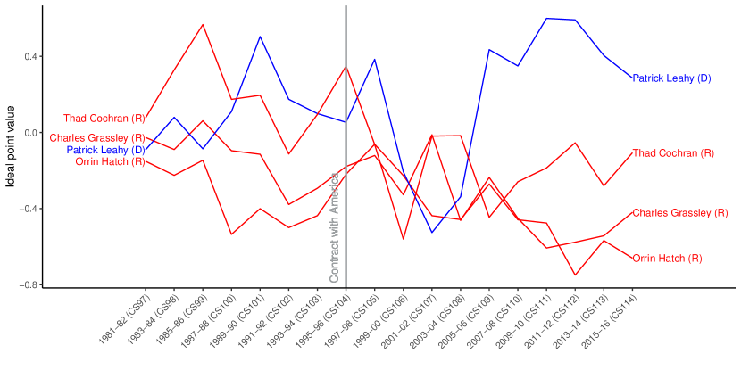
Figure 5: Development of estimated ideal points over time of those four Senators who were members of the Senate from session 97 to 114.

C.2 Comparison to DW-Nominate Scores

We determine standardized average partisanship estimates across time using the first dimension of the DW-Nominate scores and compare them with the text based average partisanship estimates from the TV-TBIP model. The session-specific average partisanship as induced by the DW-Nominate scores is obtained as the difference between the average DW-Nominate scores of Republicans and Democrats for each session.

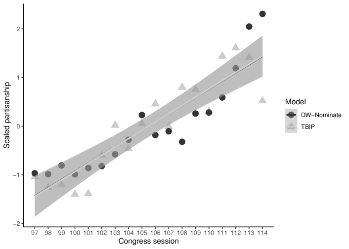
Figure 6: Standardized aggregate partisanship estimates on party level based on DW-Nominate scores and the TV-TBIP ideal points across time together with fitted linear regression lines and corresponding 95% confidence intervals for the means. The correlation between these partisanship estimates is $0.77$.

Figure 6 provides scatter plots of the time points on the $x$-axis versus the standardized average partisanship estimates for the TV-TBIP model as well as the DW-Nominate scores on the $y$-axis. Clearly both measures exhibit a similar increase over time. This is also indicated by the overlap of the fitted regression lines and their 95% confidence intervals for the mean which are also included in the plot. This implies that our text based average partisanship measure captures the same effect over time as the DW-Nominate scores.

References

- Abadi et al. (2015) Abadi M, Agarwal A, Barham P, Brevdo E, Chen Z, Citro C, Corrado GS, Davis A, Dean J, Devin M, Ghemawat S, Goodfellow I, Harp A, Irving G, Isard M, Jia Y, Jozefowicz R, Kaiser L, Kudlur M, Levenberg J, Mané D, Monga R, Moore S, Murray D, Olah C, Schuster M, Shlens J, Steiner B, Sutskever I, Talwar K, Tucker P, Vanhoucke V, Vasudevan V, Viégas F, Vinyals O, Warden P, Wattenberg M, Wicke M, Yu Y, Zheng X (2015). “TensorFlow: Large-Scale Machine Learning on Heterogeneous Systems.” Software available from tensorflow.org, URL https://tensorflow.org/.
- Bailey et al. (2005) Bailey MA, Kamoie B, Maltzman F (2005). “Signals From the Tenth Justice: The Political Role of the Solicitor General in Supreme Court Decision Making.” American Journal of Political Science, 49(1), 72–85.
- Blei et al. (2017) Blei DM, Kucukelbir A, McAuliffe JD (2017). “Variational Inference: A Review for Statisticians.” Journal of the American Statistical Association, 112(518), 859–877. 10.1080/01621459.2017.1285773.
- Blei et al. (2003) Blei DM, Ng AY, Jordan MI (2003). “Latent Dirichlet Allocation.” Journal of Machine Learning Research, 3, 993–1022.
- Boche et al. (2018) Boche A, Lewis JB, Rudkin A, Sonnet L (2018). “The New Voteview.com: Preserving and Continuing Keith Poole’s Infrastructure for Scholars, Students and Observers of Congress.” Public Choice, 176, 17–32.
- Canny (2004) Canny J (2004). “GaP: A Factor Model for Discrete Data.” In Proceedings of the 27th Annual International ACM SIGIR Conference on Research and Development in Information Retrieval, SIGIR ’04, pp. 122–129.
- Clinton and Lewis (2008) Clinton JD, Lewis DE (2008). “Expert Opinion, Agency Characteristics, and Agency Preferences.” Political Analysis, 16(1), 3–20.
- Enten (2014) Enten H (2014). “The GOP Senator Most Likely to Falter in the Primary Season.” https://fivethirtyeight.com/features/the-gop-senator-most-likely-to-falter-in-the-primary-season/. FiveThirtyEight.
- Entman (1993) Entman RM (1993). “Framing: Towards Clarification of a Fractured Paradigm.” Journal of Communication, 43(4), 51–58.
- Gentzkow et al. (2019a) Gentzkow M, Kelly B, Taddy M (2019a). “Text as Data.” Journal of Economic Literature, 57(3), 535–574. 10.1257/jel.20181020.
- Gentzkow et al. (2018) Gentzkow M, Shapiro JM, Taddy M (2018). “Congressional Record for the 43rd–114th Congresses: Parsed Speeches and Phrase Counts.” https://data.stanford.edu/congress_text. Stanford Libraries [distributor], 2018-01-16.
- Gentzkow et al. (2019b) Gentzkow M, Shapiro JM, Taddy M (2019b). “Measuring Group Differences in High-Dimensional Choices: Method and Application to Congressional Speech.” Econometrica, 87(4), 1307–1340. 10.3982/ecta16566.
- Gopalan et al. (2014) Gopalan PK, Charlin L, Blei D (2014). “Content-Based Recommendations with Poisson Factorization.” In Z Ghahramani, M Welling, C Cortes, N Lawrence, KQ Weinberger (eds.), Advances in Neural Information Processing Systems, volume 27. Curran Associates, Inc. URL https://proceedings.neurips.cc/paper/2014/file/97d0145823aeb8ed80617be62e08bdcc-Paper.pdf.
- Harris (1954) Harris ZS (1954). “Distributional Structure.” Word, 10(2-3), 146–162. 10.1080/00437956.1954.11659520.
- Holmes (2008) Holmes SA (2008). “Jesse Helms Dies at 86; Conservative Force in the Senate.” https://www.nytimes.com/2008/07/05/us/politics/00helms.html. The New York Times.
- Kingma and Ba (2015) Kingma DP, Ba JL (2015). “Adam: A Method for Stochastic Optimization.” In Proceedings of the 3rd International Conference for Learning Representations (ICLR).
- Laver et al. (2003) Laver M, Benoit K, Garry J (2003). “Extracting Policy Positions from Political Texts Using Words as Data.” American Political Science Review, 97(2), 311–331. 10.1017/s0003055403000698.
- Lee and Seung (1999) Lee D, Seung H (1999). “Learning the Parts of Objects by Non-Negative Matrix Factorization.” Nature, 401, 788–791. 10.1038/44565.
- Lewis et al. (2022) Lewis JB, Poole K, Rosenthal H, Boche A, Rudkin A, Sonnet L (2022). “Voteview: Congressional Roll-Call Votes Database.” https://voteview.com/. Online; accessed 7-February-2022.
- McCarty et al. (1997) McCarty NM, Poole KT, Rosenthal H (1997). Income Redistribution and the Realignment of American Politics. SEI Press, Washington, DC.
- Noden (2007) Noden R (2007). “Is AIDS God’s Judgment Against Homosexuality? An Argument from Natural Law.” https://digitalcommons.cedarville.edu/cedar_ethics_online/24. CedarEthics Online.
- Parlapiano and Benzaquen (2017) Parlapiano A, Benzaquen M (2017). “Where Senators Stand on the Health Care Bill.” https://www.nytimes.com/interactive/2017/06/22/us/politics/senate-health-care-whip-count.html. The New York Times [Online; published 7-July-2017].
- Pedregosa et al. (2011) Pedregosa F, Varoquaux G, Gramfort A, Michel V, Thirion B, Grisel O, Blondel M, Prettenhofer P, Weiss R, Dubourg V, Vanderplas J, Passos A, Cournapeau D, Brucher M, Perrot M, Duchesnay E (2011). “scikit-learn: Machine Learning in Python.” Journal of Machine Learning Research, 12, 2825–2830.
- Peress (2022) Peress M (2022). “Large-Scale Ideal Point Estimation.” Political Analysis, 30(3), 346–363. 10.1017/pan.2021.5.
- Poole et al. (2011) Poole K, Lewis JB, Lo J, Carroll R (2011). “Scaling Roll Call Votes with wnominate in R.” Journal of Statistical Software, 42(14), 1–21. 10.18637/jss.v042.i14.
- Poole and Rosenthal (1985) Poole KT, Rosenthal H (1985). “A Spatial Model for Legislative Roll Call Analysis.” American Journal of Political Science, 29(2), 357–384. 10.2307/2111172.
- Roberts et al. (2016) Roberts ME, Stewart BM, Airoldi EM (2016). “A Model of Text for Experimentation in the Social Sciences.” Journal of the American Statistical Association, 111(515), 988–1003. 10.1080/01621459.2016.1141684.
- Roberts et al. (2019) Roberts ME, Stewart BM, Tingley D (2019). “stm: An R Package for Structural Topic Models.” Journal of Statistical Software, 91(2), 1–40. 10.18637/jss.v091.i02.
- Slapin and Proksch (2008) Slapin JB, Proksch SO (2008). “A Scaling Model for Estimating Time-Series Party Positions from Texts.” American Journal of Political Science, 52, 705–722. 10.1111/j.1540-5907.2008.00338.x.
- Tolvanen et al. (2021) Tolvanen J, Tremewan J, Wagner AK (2021). “Ambiguous Platforms and Correlated Preferences: Experimental Evidence.” American Political Science Review, pp. 1–17. 10.1017/S0003055421001155.
- Vafa et al. (2020) Vafa K, Naidu S, Blei D (2020). “Text-Based Ideal Points.” In Proceedings of the 58th Annual Meeting of the Association for Computational Linguistics, pp. 5345–5357. Association for Computational Linguistics. URL https://www.aclweb.org/anthology/2020.acl-main.475.
- van Rossum et al. (2011) van Rossum G, et al. (2011). Python Programming Language. URL https://www.python.org.
- Wikipedia (2021) Wikipedia (2021). “Frank Luntz — Wikipedia, The Free Encyclopedia.” https://en.wikipedia.org/w/index.php?title=Frank_Luntz&oldid=1060333953. [Online; accessed 7-February-2022].
- Wikipedia (2022a) Wikipedia (2022a). “Contract with America — Wikipedia, The Free Encyclopedia.” https://en.wikipedia.org/w/index.php?title=Contract_with_America&oldid=1067380696. [Online; accessed 7-February-2022].
- Wikipedia (2022b) Wikipedia (2022b). “Gordon H. Smith — Wikipedia, The Free Encyclopedia.” https://en.wikipedia.org/w/index.php?title=Gordon_H._Smith&oldid=1067141497. [Online; accessed 9-February-2022].
- Wikipedia (2022c) Wikipedia (2022c). “Orrin Hatch — Wikipedia, The Free Encyclopedia.” https://en.wikipedia.org/w/index.php?title=Orrin_Hatch&oldid=1080711278. [Online; accessed 5-April-2022].