Classical and quantum bicosmology with noncommutativity

Abstract

Recently, Falomir, Gamboa, Méndez, Gondolo and Maldonado proposed a bicosmology scenario FGMG ; FGGM ; FGM ; MM for solving some cosmological problems related to inflation, dark matter, and thermal history of the universe. Their plan is to introduce noncommutativity into the momentum space of the two scale factors. In the present paper, we revisit their model and first consider exact classical solutions in the model with constant noncommutativity between dynamical variables and between canonical momenta. We also hypothesize that the noncommutativity appears when the scale factors are small, and show the behavior of the classical solution in that case with momentum-space noncommutativity. Finally, we write down the Wheeler–DeWitt equation in that case and examine the behavior of the solution.

I Introduction

The bicosmology scenario has been proposed by Falomir, Gamboa, Méndez, Gondolo and Maldonado FGMG ; FGGM ; FGM ; MM . In their scenario, two scale factors are introduced to represent two causally separated regions of a universe, or even two different universes in a multiverse scenario MM . From a different point of view, it can be regarded as a kind of cosmological models in bigravity theory (for example, see Refs. AM ; SS ; DM ). However, instead of the mass term by mixing of two scale factors in bigravity, mixing is guaranteed to be due to the noncommutativity in the Hamiltonian formulation of the classical bicosmology.

Noncommutative cosmology has been studied by many authors COR1 ; BP ; PM ; PO ; AAOSS ; GSS1 ; GSS2 ; GSS3 ; MOS1 ; MOS2 ; OMSS ; SPOA ; BBDP1 ; BBDP2 ; BBDP3 ; MMP ; OQ ; RM1 ; RM2 ; RZJM ; JCM ; RSFMM ; RMM ; KKST2 ; JRN ; COR2 ; Rasouli , not only classically but also quantum mechanically. Thus, we intend to study various aspects of classical and quantum bicosmology.

In the present paper, we revisit the model of bicosmology and examine classical and quantum cosmological solutions. Although the main analyses in the later sections will be illustrated when canonical momenta are noncommutative, we also consider noncommutativity in dynamical variables in the minisuperspace at first.

Next, we observe the case where the parameter representing the noncommutativity is not constant. The most natural idea is that noncommutativity has little effect on the cosmological evolution when the universe is large, but is highly effective at the very early stage of the universe, when the universe is small. We also write down the Wheeler–DeWitt (WDW) equation for that case and study the behavior of the solution.

Sec. II describes setting up the model for bicosmology and obtaining classical solutions for the commutative case. In Sec. III, we study classical bicosmology with noncommutativity in the phase space. In Sec. IV, we define the nonconstant noncommutativity in momentum space and investigate classical solutions in the system. Quantum bicosmology by the WDW equation in the system is studied in Sec. V. Finally, conclusion and discussion are given in the last section.

II commutative bicosmology model

We consider the following action consisting only of the Einstein–Hilbert term and the cosmological term:

$$S\propto\int d^{D}x\sqrt{-g}\Bigl{[}R-2\Lambda\Bigr{]}\,,$$ (1)

where $R$ is the Ricci scalar derived from the metric $g_{\mu\nu}$ ($\mu,\nu=0,1,\ldots,D-1$), and $g$ is the determinant of $g_{\mu\nu}$. We also assumed that the cosmological constant $\Lambda$ is a positive constant. As a first step in an analysis, it is very important to investigate cases where such toy models have exact solutions. It will also be useful for consideration on numerical analyses of sophisticated models with further variations in the future.

First, in this section we will review the commutative version of the bicosmology, which we will use later for comparison with the noncommutative case.

We take an ansatz for the metric tensor as

$$ds^{2}=g_{\mu\nu}dx^{\mu}dx^{\nu}=-N^{2}dt^{2}+a^{2}(t)d\mathbf{x}^{2}\,,$$ (2)

where $t=x^{0}$, $d\mathbf{x}^{2}\equiv\sum_{i=1}^{D-1}(dx^{i})^{2}$, and $N$ stands for the lapse function. Then, one can derive the following Lagrangian for the scale factor from the action (1):

$$L=-\frac{1}{2N}a^{{D-3}}\dot{a}^{2}-\frac{N}{(D-1)(D-2)}\Lambda a^{D-1}\,,$$ (3)

where the dot indicates the derivative with respect to time $t$ and total derivatives have been dropped. Now, we switch the dynamical variable $a$ to $x$, which is defined as

$$x\equiv\frac{2}{D-1}a^{\frac{D-1}{2}}\,.$$ (4)

Then, the Lagrangian takes the form

$$L=-\frac{1}{2N}\dot{x}^{2}-\frac{N}{2}\gamma^{2}x^{2}\,,$$ (5)

where

$$\gamma^{2}=\frac{D-1}{2(D-2)}\Lambda\,.$$ (6)

Note that this Lagrangian is just that of an inverted harmonic oscillator.

In the bicosmology scenario FGMG ; FGGM ; FGM ; MM , the second scale factor $b$, which represents the causally disconnected region, is introduced. Here, we adopt the case that the Lagrangian for the second scale factor $b$ is just a copy of that for the first scale factor $a$, though the authors of Refs. FGMG ; FGGM ; FGM ; MM considered generally different values for cosmological constants. Therefore, the total Lagrangian takes the form of the two-dimensional inverted harmonic oscillator:

$$L=-\frac{1}{2N}(\dot{x}^{2}+\dot{y}^{2})-\frac{N}{2}\gamma^{2}(x^{2}+y^{2})\,,$$ (7)

where

$$y=\frac{2}{D-1}b^{\frac{D-1}{2}}\,.$$ (8)

To construct the Hamiltonian, we have only to follow the standard method. The conjugate momenta are found to be

$$\pi_{x}\equiv\frac{\partial L}{\partial\dot{x}}=-\frac{\dot{x}}{N}\,,\qquad\pi_{y}\equiv\frac{\partial L}{\partial\dot{y}}=-\frac{\dot{y}}{N}\,,$$ (9)

and the Hamiltonian is finally obtained as

$$H=N\left[-\frac{1}{2}(\pi_{x}^{2}+\pi_{y}^{2})+\frac{1}{2}\gamma^{2}(x^{2}+y^{2})\right]\,,$$ (10)

which is the Hamiltonian for the two-dimensional inverted harmonic oscillator (up to the lapse function).

The Hamiltonian constraint is assigned from $\frac{\partial H}{\partial N}=0$. We thus set $N=1$ hereafter.

The Poisson brackets are placed as usual:

$$\{x,\pi_{x}\}=\{y,\pi_{y}\}=1\,,$$ (11)

and others are zero. Then, the usual Hamilton’s equations are obtained as

$$\dot{x}=\{x,H\}=\frac{\partial H}{\partial\pi_{x}}=-\pi_{x}\,,\quad\dot{y}=\{y,H\}=\frac{\partial H}{\partial\pi_{y}}=-\pi_{y}\,,$$

$$\dot{\pi}_{x}=\{\pi_{x},H\}=-\frac{\partial H}{\partial x}=-\gamma^{2}x\,,\quad\dot{\pi}_{y}=\{\pi_{y},H\}=-\frac{\partial H}{\partial y}=-\gamma^{2}y\,,$$ (12)

and subsequently, we can derive the equations of motion as

$$\ddot{x}-\gamma^{2}x=0\,,\quad\ddot{y}-\gamma^{2}y=0\,.$$ (13)

The solution of the equations is

$$x(t) = C_{1}\cos\varphi_{0}\exp[\gamma t]+C_{2}\sin\varphi_{0}\exp[-\gamma t]\,,$$ (14)

$$y(t) = C_{1}\sin\varphi_{0}\exp[\gamma t]-C_{2}\cos\varphi_{0}\exp[-\gamma t]\,,$$ (15)

where the arrangement of the constant coefficients $C_{1}$, $C_{2}$, and the constant phase angle $\varphi_{0}$ have been chosen as the Hamiltonian constraint $H=0$ holds. These exponential behaviors are expected from the inverse harmonic oscillator Hamiltonian.

With the preparatory calculations complete, in the next section we consider classical noncommutative bicosmology.

III Classical noncommutative bicosmology

The authors of bicosmology FGMG ; FGGM ; FGM ; MM introduced noncommutativity into the momentum space of the system. We first consider noncommutative dynamical variables as well.

We presume that the corresponding noncommutative system is defined by replacement

$$x\rightarrow X\,,\quad\pi_{x}\rightarrow\Pi_{X}\,,\quad y\rightarrow Y\,,\quad\pi_{y}\rightarrow\Pi_{Y}\,,$$ (16)

and the Hamiltonian takes the form of the inverted harmonic oscillator,

$$H_{NC}=-\frac{1}{2}(\Pi_{X}^{2}+\Pi_{Y}^{2})+\frac{1}{2}\gamma^{2}(X^{2}+Y^{2})\,.$$ (17)

Here, we assume the noncommutative phase space in the minisuperspace, which is realized by the deformed Poisson brackets

$$\{X,\Pi_{X}\}=\{Y,\Pi_{Y}\}=1\,,\quad\{X,Y\}=\Theta\,,\quad\{\Pi_{X},\Pi_{Y}\}=B\,,$$ (18)

and others are zero. We assume the parameters which represent noncommutativities, $\Theta$ and $B$, are constant for this time.

Now, the canonical equations can be obtained as

$$\dot{X}=\{X,H_{NC}\}=-\Pi_{X}+\gamma^{2}\Theta Y\,,\quad\dot{Y}=\{Y,H_{NC}\}=-\Pi_{Y}-\gamma^{2}\Theta X\,,$$

$$\dot{\Pi}_{X}=\{\Pi_{X},H_{NC}\}=-\gamma^{2}X-B\Pi_{Y}\,,\quad\dot{\Pi}_{Y}=\{\Pi_{Y},H_{NC}\}=-\gamma^{2}Y+B\Pi_{X}\,,$$ (19)

and consequently, the equations of motion for $X$ and $Y$ can be revealed as

$$\ddot{X}-(\gamma^{2}\Theta-B)\dot{Y}-\gamma^{2}(1-B\Theta)X=0\,,\quad\ddot{Y}+(\gamma^{2}\Theta-B)\dot{X}-\gamma^{2}(1-B\Theta)Y=0\,.$$ (20)

These equations can be easily solved, especially if we considered a combination

$$\ddot{Z}+i(\gamma^{2}\Theta-B)\dot{Z}-\gamma^{2}(1-B\Theta)Z=0\,,$$ (21)

where $Z\equiv X+iY$.

The general solutions which satisfy the Hamiltonian constraint $H_{NC}=0$ are exhibited as follows.

$\bullet$ if $|B+\gamma^{2}\Theta|<2\gamma$

$$X(t) = C_{1}\exp\Biggl{[}\frac{\sqrt{4\gamma^{2}-(\gamma^{2}\Theta+B)^{2}}}{2}t\Biggr{]}\cos\Biggl{[}\frac{B-\gamma^{2}\Theta}{2}t+\varphi_{1}\Biggr{]}$$ (22)

$$+ C_{2}\exp\Biggl{[}-\frac{\sqrt{4\gamma^{2}-(\gamma^{2}\Theta+B)^{2}}}{2}t\Biggr{]}\sin\Bigl{[}\frac{B-\gamma^{2}\Theta}{2}t+\varphi_{2}\Bigr{]}\,,$$

$$Y(t) = C_{1}\exp\Biggl{[}\frac{\sqrt{4\gamma^{2}-(\gamma^{2}\Theta+B)^{2}}}{2}t\Biggr{]}\sin\Biggl{[}\frac{B-\gamma^{2}\Theta}{2}t+\varphi_{1}\Biggr{]}$$ (23)

$$- C_{2}\exp\Biggl{[}-\frac{\sqrt{4\gamma^{2}-(\gamma^{2}\Theta+B)^{2}}}{2}t\Biggr{]}\cos\Biggl{[}\frac{B-\gamma^{2}\Theta}{2}t+\varphi_{2}\Biggr{]}\,,$$

where $C_{1}$, $C_{2}$, $\varphi_{1}$, and $\varphi_{2}$ are constants. The two phase angles should satisfy

$$\sin(\varphi_{2}-\varphi_{1})=\frac{B+\gamma^{2}\Theta}{2\gamma}\,,$$ (24)

for the Hamiltonian constraint.

$\bullet$ if $|B+\gamma^{2}\Theta|=2\gamma$

$$X(t) = C\cos\Biggl{[}\frac{B-\gamma^{2}\Theta}{2}t+\varphi_{1}\Biggr{]}$$ (25)

$$+ C(B+\gamma^{2}\Theta)\sin(\varphi_{1}-\varphi_{2})\cdot t\cos\Biggl{[}\frac{B-\gamma^{2}\Theta}{2}t+\varphi_{2}\Biggr{]}\,,$$

$$Y(t) = C\sin\Biggl{[}\frac{B-\gamma^{2}\Theta}{2}t+\varphi_{1}\Biggr{]}$$ (26)

$$+ C(B+\gamma^{2}\Theta)\sin(\varphi_{1}-\varphi_{2})\cdot t\sin\Biggl{[}\frac{B-\gamma^{2}\Theta}{2}t+\varphi_{2}\Biggr{]}\,,$$

where $C$, $\varphi_{1}$, and $\varphi_{2}$ are constants.

$\bullet$ if $|B+\gamma^{2}\Theta|>2\gamma$

$$X(t) = Ce^{-\eta}\cos\Biggl{[}\frac{B-\gamma^{2}\Theta+\sqrt{(B+\gamma^{2}\Theta)^{2}-4\gamma^{2}}}{2}t+\varphi_{1}\Biggr{]}$$ (27)

$$+ Ce^{\eta}\sin\Biggl{[}\frac{B-\gamma^{2}\Theta-\sqrt{(B+\gamma^{2}\Theta)^{2}-4\gamma^{2}}}{2}t+\varphi_{2}\Biggr{]}\,,$$

$$Y(t) = Ce^{-\eta}\sin\Biggl{[}\frac{B-\gamma^{2}\Theta+\sqrt{(B+\gamma^{2}\Theta)^{2}-4\gamma^{2}}}{2}t+\varphi_{1}\Biggr{]}$$ (28)

$$- Ce^{\eta}\cos\Biggl{[}\frac{B-\gamma^{2}\Theta-\sqrt{(B+\gamma^{2}\Theta)^{2}-4\gamma^{2}}}{2}t+\varphi_{2}\Biggr{]}\,,$$

where $C$, $\varphi_{1}$, and $\varphi_{2}$ are constants. The constant $\eta$ is determined by

$$\cosh(2\eta)=\frac{|B+\gamma^{2}\Theta|}{2\gamma}\,.$$ (29)

All these noncommutative classical solutions are always involve trigonometric functions, with each scale factor going to zero at some point in the past or the future. The case with $B=\gamma^{2}\Theta$ is interesting because it has no slow oscillatory behavior, but we naturally think that $B$ and $\gamma^{2}\Theta$ do not take large values at present, and they are expected to be much less than $H_{0}$ (the Hubble constant), so they do not affect the current expansion of the universe. Therefore, the relation $B\sim\gamma^{2}\Theta$ need not be taken too seriously. Interestingly, however, it is possible that the parameters of the noncommutativity became large only in the early stage of the small universe. We explore this possibility in the next section.

Incidentally, $X^{2}+Y^{2}$ in each case is found to be

$$X^{2}+Y^{2} = C_{1}^{2}\exp\Bigl{[}{\sqrt{4\gamma^{2}-(\gamma^{2}\Theta+B)^{2}}}t\Bigr{]}+C_{2}^{2}\exp\Bigl{[}-{\sqrt{4\gamma^{2}-(\gamma^{2}\Theta+B)^{2}}}t\Bigr{]}$$ (30)

$$+2C_{1}C_{2}\frac{B+\gamma^{2}\Theta}{2\gamma}\,,\qquad\qquad\qquad\qquad\qquad\qquad(|B+\gamma^{2}\Theta|<2\gamma)$$

$$X^{2}+Y^{2} = C^{2}\Bigl{[}1+2(B+\gamma^{2}\Theta)\sin(\varphi_{1}-\varphi_{2})\cos(\varphi_{1}-\varphi_{2})\cdot t$$ (31)

$$\qquad+(B+\gamma^{2}\Theta)^{2}\sin^{2}(\varphi_{1}-\varphi_{2})\cdot t^{2}\Bigr{]}\,,\qquad\qquad(|B+\gamma^{2}\Theta|=2\gamma)$$

$$X^{2}+Y^{2} = 2C^{2}\Biggl{[}\frac{|B+\gamma^{2}\Theta|}{2\gamma}-\sin[\sqrt{(B+\gamma^{2}\Theta)^{2}-4\gamma^{2}}t+\varphi_{1}-\varphi_{2}]\Biggr{]}\,.$$ (32)

$$\hskip 240.0pt(|B+\gamma^{2}\Theta|>2\gamma)$$

It can be seen that $X^{2}+Y^{2}$ does not oscillate slowly, except for the rapid oscillation for $|B+\gamma^{2}\Theta|>2\gamma$, so it can be a measure of the average size of the two scale factors at least, but its physical meaning should be discussed in later sections.

In the rest of this section, we will note the formulation of noncommutative system using undeformed canonical variables. A similar formulation is already known in quantum cosmology, the technique required to find the WDW equation COR1 ; BP ; PM ; PO ; AAOSS ; GSS1 ; GSS2 ; GSS3 ; MOS1 ; MOS2 ; OMSS ; SPOA ; BBDP1 ; BBDP2 ; BBDP3 ; MMP ; OQ ; KKST2 ; JRN ; COR2 .

For this, we set the variables as follows:

$$X=\frac{1}{\sqrt{1+\frac{\beta\theta}{4}}}\Bigl{(}x-\frac{\theta}{2}\pi_{y}\Bigr{)}\,,\quad Y=\frac{1}{\sqrt{1+\frac{\beta\theta}{4}}}\Bigl{(}y+\frac{\theta}{2}\pi_{x}\Bigr{)}\,,$$

$$\Pi_{X}=\frac{1}{\sqrt{1+\frac{\beta\theta}{4}}}\Bigl{(}\pi_{x}+\frac{\beta}{2}y\Bigr{)}\,,\quad\Pi_{Y}=\frac{1}{\sqrt{1+\frac{\beta\theta}{4}}}\Bigl{(}\pi_{y}-\frac{\beta}{2}x\Bigr{)}\,,$$ (33)

where $x$, $\pi_{x}$, $y$, and $\pi_{y}$ obey the usual Poisson brackets (11). If the constant parameters $\theta$ and $\beta$ are related to $\Theta$ and $B$ as

$$\Theta=\frac{\theta}{1+\frac{\beta\theta}{4}}\,,\quad B=\frac{\beta}{1+\frac{\beta\theta}{4}}\,,$$ (34)

one can find that the brackets for $X$, $\Pi_{X}$, $Y$, $\Pi_{Y}$ defined by (33) realize the noncommutative Poisson brackets (18). Then, the Hamiltonian $H_{NC}$ is expressed as

$$H_{NC}=-\frac{1-\frac{\gamma^{2}\theta^{2}}{4}}{2\left(1+\frac{\beta\theta}{4}\right)}(\pi_{x}^{2}+\pi_{y}^{2})+\frac{\beta-\gamma^{2}\theta}{2\left(1+\frac{\beta\theta}{4}\right)}(x\pi_{y}-y\pi_{x})+\frac{\gamma^{2}-\frac{\beta^{2}}{4}}{2\left(1+\frac{\beta\theta}{4}\right)}(x^{2}+y^{2})\,.$$ (35)

The equivalence of the equations motion can be checked easily. Since one can see

$$\dot{x}=\frac{\partial H_{NC}}{\partial\pi_{x}}=-\frac{1-\frac{\gamma^{2}\theta^{2}}{4}}{1+\frac{\beta\theta}{4}}\pi_{x}-\frac{\beta-\gamma^{2}\theta}{2(1+\frac{\beta\theta}{4})}y\,,$$

$$\dot{y}=\frac{\partial H_{NC}}{\partial\pi_{y}}=-\frac{1-\frac{\gamma^{2}\theta^{2}}{4}}{1+\frac{\beta\theta}{4}}\pi_{y}+\frac{\beta-\gamma^{2}\theta}{2(1+\frac{\beta\theta}{4})}x\,,$$

$$\dot{\pi}_{x}=-\frac{\partial H_{NC}}{\partial x}=-\frac{\gamma^{2}-\frac{\beta^{2}}{4}}{1+\frac{\beta\theta}{4}}x-\frac{\beta-\gamma^{2}\theta}{2(1+\frac{\beta\theta}{4})}\pi_{y}\,,$$

$$\dot{\pi}_{y}=-\frac{\partial H_{NC}}{\partial y}=-\frac{\gamma^{2}-\frac{\beta^{2}}{4}}{1+\frac{\beta\theta}{4}}y+\frac{\beta-\gamma^{2}\theta}{2(1+\frac{\beta\theta}{4})}\pi_{x}\,,$$ (36)

one can finally find the identical equations with (19),

$$\dot{X}=\frac{1}{\sqrt{1+\frac{\beta\theta}{4}}}\Bigl{(}\dot{x}-\frac{\theta}{2}\dot{\pi}_{y}\Bigr{)}=-\Pi_{X}+\gamma^{2}\Theta Y\,,$$

$$\dot{Y}=\frac{1}{\sqrt{1+\frac{\beta\theta}{4}}}\Bigl{(}\dot{y}+\frac{\theta}{2}\dot{\pi}_{x}\Bigr{)}=-\Pi_{Y}-\gamma^{2}\Theta X\,,$$

$$\dot{\Pi}_{X}=\frac{1}{\sqrt{1+\frac{\beta\theta}{4}}}\Bigl{(}\dot{\pi}_{x}+\frac{\beta}{2}\dot{y}\Bigr{)}=-\gamma^{2}X-B\Pi_{Y}\,,$$

$$\dot{\Pi}_{Y}=\frac{1}{\sqrt{1+\frac{\beta\theta}{4}}}\Bigl{(}\dot{\pi}_{y}-\frac{\beta}{2}\dot{x}\Bigr{)}=-\gamma^{2}Y+B\Pi_{X}\,.$$ (37)

Then, the check is completed as mentioned above.

IV noncommutativity in momenta for small scale factors: Classical system

If the parameter $\theta=0$, (33) is simplified as

$$X=x\,,\quad Y=y\,,\quad\Pi_{X}=\pi_{x}+\frac{\beta}{2}y\,,\quad\Pi_{Y}=\pi_{y}-\frac{\beta}{2}x\,.$$ (38)

This is exactly what the authors of Refs. FGMG ; FGGM ; FGM ; MM considered. With the noncommutativity of the canonical momenta, this model has several advantages over simplicity. One advantage is that configuration variables $X$ and $Y$ are trivially represented by $x$ and $y$. In particular, for the study of noncommutative quantum cosmology in general, it is necessary to derive the Wigner function Wigner ; Case ; WF to analyze the solution of WDW equation for $\{X,Y\}\neq 0$ (see Ref. KKST2 for example). Even with the classical model of cosmology, the analysis becomes tedious, at least in general cases. Models involving general noncommutativity in phase spaces of the minisuperspaces are left for future work.

Another advantage of considering only the nontrivial Poisson bracket $\{\Pi_{X},\Pi_{Y}\}\neq 0$ is the analogy with a magnetic flux FGMG ; FGGM ; FGM ; MM . In Ref. FGGM , the authors explicitly pointed to the quantum Hall effect as a similar system.

Here, in the present paper, we propose nonconstant noncommutativity in the minisuperspace. As already mentioned, the noncommutativity is thought to have no effect in the present epoch, but it may have a large effect in the early universe when the scale factors are very small.

Now, suppose that the parameter $\beta$ in (38) is a function of $r=\sqrt{x^{2}+y^{2}}$. Accordingly, the Poisson bracket of $\Pi_{X}$ and $\Pi_{Y}$ becomes

$$\{\Pi_{X},\Pi_{Y}\}=\beta(r)+\frac{r\beta^{\prime}(r)}{2}\,,$$ (39)

where the prime denotes the derivative with respect to $r$. Thus, the relation between $\beta$ and $B$ is slightly modified if there are position dependence in the minisuperspace.

The Hamiltonian (17) now takes the form

$$H_{NC}=-\frac{1}{2}(\pi_{x}^{2}+\pi_{y}^{2})+\frac{1}{2}\beta(r)(x\pi_{y}-y\pi_{x})+\frac{1}{2}\left(\gamma^{2}-\frac{\beta^{2}(r)}{4}\right)(x^{2}+y^{2})\,.$$ (40)

The canonical equations

$$\dot{x}=\frac{\partial H_{NC}}{\partial\pi_{x}}=-\pi_{x}-\frac{\beta(r)}{2}y\,,\quad\dot{y}=\frac{\partial H_{NC}}{\partial\pi_{y}}=-\pi_{y}+\frac{\beta(r)}{2}x\,,$$

$$\dot{\pi}_{x}=-\frac{\partial H_{NC}}{\partial x}=-\left(\gamma^{2}-\frac{\beta(r)(\beta(r)+r\beta^{\prime}(r))}{4}\right)x-\frac{\beta(r)}{2}\pi_{y}-\frac{\beta^{\prime}(r)x}{2r}(x\pi_{y}-y\pi_{x})\,,$$

$$\dot{\pi}_{y}=-\frac{\partial H_{NC}}{\partial y}=-\left(\gamma^{2}-\frac{\beta(r)(\beta(r)+r\beta^{\prime}(r))}{4}\right)y+\frac{\beta(r)}{2}\pi_{x}-\frac{\beta^{\prime}(r)y}{2r}(x\pi_{y}-y\pi_{x})\,,$$ (41)

leads to the following equations of motion:

$$\ddot{x}+\beta\dot{y}+\frac{\beta^{\prime}}{2r}(x\dot{x}+y\dot{y})y-\left(\gamma^{2}-\frac{r\beta\beta^{\prime}}{4}\right)x+\frac{\beta^{\prime}}{2r}\left[x\dot{y}-y\dot{x}-\frac{\beta}{2}(x^{2}+y^{2})\right]x=0\,,$$ (42)

$$\ddot{y}-\beta\dot{x}-\frac{\beta^{\prime}}{2r}(x\dot{x}+y\dot{y})x-\left(\gamma^{2}-\frac{r\beta\beta^{\prime}}{4}\right)y+\frac{\beta^{\prime}}{2r}\left[x\dot{y}-y\dot{x}-\frac{\beta}{2}(x^{2}+y^{2})\right]y=0\,.$$ (43)

By use of the polar coordinates

$$X=x=r\cos\phi\,,\quad Y=y=r\sin\phi\,,$$ (44)

the equations of motion reduce to

$$\ddot{r}-r\dot{\phi}^{2}+\beta\,r\dot{\phi}-\gamma^{2}r+\frac{\beta^{\prime}}{2}r^{2}\dot{\phi}$$ (46)

$$= \ddot{r}-r\left(\dot{\phi}-\frac{\beta}{2}\right)^{2}-\left(\gamma^{2}-\frac{\beta(\beta+r\beta^{\prime})}{4}\right)r+\frac{\beta^{\prime}}{2}r^{2}\left(\dot{\phi}-\frac{\beta}{2}\right)=0\,,$$

$$r\ddot{\phi}+2\dot{r}\dot{\phi}-\beta\,\dot{r}-\frac{\beta^{\prime}}{2}r\dot{r}=\frac{1}{r}\frac{d}{dt}\left[r^{2}\left(\dot{\phi}-\frac{\beta}{2}\right)\right]=0\,.$$

On the other hand, the Hamiltonian constraint reads

$$H_{NC} = -\frac{1}{2}\dot{r}^{2}-\frac{1}{2}r^{2}\dot{\phi}^{2}+\frac{1}{2}\gamma^{2}r^{2}$$ (47)

$$= -\frac{1}{2}\dot{r}^{2}-\frac{1}{2}r^{2}\left(\dot{\phi}-\frac{\beta}{2}\right)^{2}-\frac{\beta}{2}r^{2}\left(\dot{\phi}-\frac{\beta}{2}\right)+\frac{1}{2}\left(\gamma^{2}-\frac{\beta^{2}}{4}\right)r^{2}=0\,.$$

The equation (46) can be integrated and if we set

$$L=r^{2}\left(\dot{\phi}-\frac{\beta(r)}{2}\right)=\mbox{constant}\,,$$ (48)

the constraint equation becomes

$$\dot{r}^{2}+\frac{L^{2}}{r^{2}}+{L\beta(r)}-\left(\gamma^{2}-\frac{\beta^{2}(r)}{4}\right)r^{2}=0\,,$$ (49)

or, equivalently

$$\dot{r}^{2}=\gamma^{2}r^{2}-\left(\frac{L}{r}+\frac{r\beta(r)}{2}\right)^{2}\,.$$ (50)

Now, we find that the equations of motion can be integrated and have very simple forms even if $\beta$ is not constant as long as $\beta$ is an arbitrary function of $r$ only.

We would like to show a concrete example of the solution. For this purpose, we adopt the following form of $\beta(r)$:

$$\beta(r)=\frac{\beta_{0}}{1+e^{\mu(r-r_{c})}}\,,$$ (51)

where $\beta_{0}$, $\mu$, and $r_{c}$ are positive constants. This typical form shows that $\beta\sim\beta_{0}$ for $r<r_{c}$ and $\beta\sim 0$ for $r>r_{c}$, i.e., $\beta$ is finite in the vicinity of the origin of the minisuperspace, $X=Y=0$. This form mimics a solenoid of radius $r_{c}$. In Fig. 1, we are trying to compare the noncommutative and the commutative cases. In both cases, we set $\gamma=1$. For the noncommutative case, we choose $\beta_{0}=5$, $\mu=10$, and $r_{c}=1$. The evolution of $X=x$ and $Y=y$ can be clearly seen if the solutions of (46) and (50) are plotted on an $(X,Y)$ plane as shown in Fig. 1. Arrows in the figures indicate the normalized “velocity” vectors

$$\frac{1}{\sqrt{\dot{X}^{2}+\dot{Y}^{2}}}(\dot{X},\dot{Y})\,,$$ (52)

at the points. In Fig. 1, the gray curves (quarter circles) indicate that the right-hand side of (50) becomes zero.

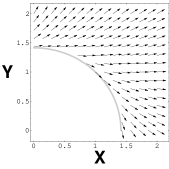
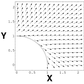
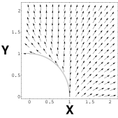
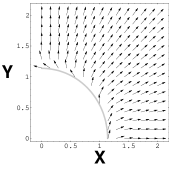
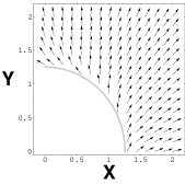
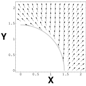
Figure 1: The normalized velocity vectors which indicate the flow of evolution of $X$ and $Y$ (see the text). (Top row) The commutative case ($\beta=0$). The figures are plotted for $L=-2,-1,0,1,2$, from left to right. (Bottom row) The case with the nonconstant noncommutativity. For the choice of parameters, see the text. The figures are plotted for $L=-2,-1,0,1,2$, from left to right.

Roughly speaking, non zero $\beta$ contributes to the “angular velocity” $\dot{\phi}$. Thus, the effective potential

$$V_{eff}(r)=-\frac{1}{2}\gamma^{2}r^{2}+\frac{1}{2}\left(\frac{L}{r}+\frac{r\beta(r)}{2}\right)^{2}\,,$$ (53)

has a positive barrier for a finite $\beta$ even if $L=0$. For negative $L$ and positive $\beta$, there appears a small region where $V_{eff}<0$ (in the region of $r<r_{c}$), so that there appears a region where the solution is approximately described by (27) and (28) (with $\Theta=0$ and $B\approx\beta_{0}$ in this time). In any case, a large enough $\beta_{0}$ can forbid the small value of $X$ and $Y$ simultaneously; In short, $r=\sqrt{X^{2}+Y^{2}}<\approx r_{c}$ is the forbidden region.

This means that the scale factors of bicosmology at the beginning of the classical universe is small but finite, in the sense of “average”, $r=\sqrt{X^{2}+Y^{2}}\approx r_{c}$. The discussion on the averaging will be shown later.

V noncommutativity in momenta for small scale factors: Quantum system

In this section, we adopt the same system as the one dealt with in the previous section, and here we consider quantum cosmology HH ; Hawking ; Halliwell ; Kiefer0 ; Kiefer1 . The WDW equation is obtained by the following replacement in the Hamiltonian constraint:

$$\pi_{x}\rightarrow-i\frac{\partial}{\partial x}\,,\quad\pi_{y}\rightarrow-i\frac{\partial}{\partial y}\,.$$ (54)

Incidentally, one can confirm the commutators

$$[X,\Pi_{X}]=[Y,\Pi_{Y}]=i\,,\quad[\Pi_{X},\Pi_{Y}]=i\left(\beta(r)+\frac{r}{2}\beta^{\prime}(r)\right)\,,$$ (55)

by using the set of operators

$$X=x\,,\quad Y=y\,,\quad\Pi_{X}=-i\frac{\partial}{\partial x}+\frac{\beta(r)}{2}y\,,\quad\Pi_{Y}=-i\frac{\partial}{\partial y}-\frac{\beta(r)}{2}x\,.$$ (56)

The WDW equation $H_{NC}\Psi=0$ in our model, which is obtained by substituting (56) into (17), can be written after the coordinate transformation (44) as,

$$\left[\frac{1}{r}\frac{\partial}{\partial r}r\frac{\partial}{\partial r}+\frac{1}{r^{2}}\frac{\partial^{2}}{\partial\phi^{2}}-i\beta(r)\frac{\partial}{\partial\phi}+\Bigl{(}\gamma^{2}-\frac{\beta^{2}(r)}{4}\Bigr{)}r^{2}\right]\Psi(r,\phi)=0\,,$$ (57)

where $\Psi$ is the so-called wave function of the universe. Note that the metric of the minisuperspace is Euclidean (not Lorentzian).

The fundamental solution for this WDW equation takes the form

$$\psi_{L}(r)e^{-iL\phi}\,,$$ (58)

and then, the function $\psi_{L}$ obeys the equation

$$\left[\frac{1}{r}\frac{\partial}{\partial r}r\frac{\partial}{\partial r}-\frac{L^{2}}{r^{2}}-L\beta(r)+\Bigl{(}\gamma^{2}-\frac{\beta^{2}(r)}{4}\Bigr{)}r^{2}\right]\psi_{L}(r)=0\,.$$ (59)

The general solution then takes the form $\Psi=\sum_{L=-\infty}^{\infty}A_{L}\psi_{L}(r)e^{-iL\phi}$, where $A_{L}$ denotes the amplitude.

For a constant $\beta$, the solution for $\psi_{L}(r)$ which is finite at $r=0$ is expressed by using the confluent hypergeometric function as BS ; SB

$$\psi_{L}(r)=r^{|L|}e^{-i\frac{\sqrt{\gamma^{2}-\frac{\beta^{2}}{4}}}{2}r^{2}}{}_{1}F_{1}\Biggl{(}\frac{|L|+1}{2}+\frac{\beta L}{4i\sqrt{\gamma^{2}-\frac{\beta^{2}}{4}}};|L|+1;i\sqrt{\gamma^{2}-\frac{\beta^{2}}{4}}r^{2}\Biggr{)}\quad(\gamma^{2}>{\beta^{2}}/{4})\,,$$ (60)

$$\psi_{L}(r)=r^{|L|}e^{-\frac{\sqrt{\frac{\beta^{2}}{4}-\gamma^{2}}}{2}r^{2}}{}_{1}F_{1}\Biggl{(}\frac{|L|+1}{2}+\frac{\beta L}{4\sqrt{\frac{\beta^{2}}{4}-\gamma^{2}}};|L|+1;\sqrt{\frac{\beta^{2}}{4}-\gamma^{2}}r^{2}\Biggr{)}\quad(\gamma^{2}<{\beta^{2}}/{4})\,.$$ (61)

Especially, for the commutative case $\beta\equiv 0$, $\psi_{L}(r)\propto J_{|L|/2}(\gamma r^{2}/2)$, where $J_{\nu}(z)$ is the Bessel function.

For relatively small values of $\beta$ and finite $L$, the first peak of the wave function $\psi_{L}$ is pushed to a larger $r$ by the “centrifugal force”.

Figure 2: The numerical solutions $\psi_{0}(r)$ ($L=0$) are plotted for $|\beta_{0}|=0,5,10,15$, from left to right. There is no scale on the vertical axis because an overall coefficient of the fundamental solution is arbitrary.

In the case with the nonconstant noncommutativity for small scale factors, proposed in the previous section, the situation is the same. The most interesting case is when $L=0$ with the nonconstant noncommutativity. In Fig. 2, we plot $\psi_{0}(r)$ for various values of $\beta_{0}$, where $\beta(r)$ is the same as (51), and $r_{c}=1$, $\mu=10$, and $\gamma=1$. This behavior can be understood by considering the effective potential $V_{eff}$ (53). As seen from Fig. 3, the noncommutativity, which exists only in the region where $r$ is small, creates the potential barrier and the first peak of the wave function is located outside $r=r_{c}$; It can be said that the wave function represents the tunneling phenomenon. The possibility that our universe start with a small but finite scale (in the present case, $r\approx r_{c}$) seems to be very interesting; The scenario is very akin to the model of early quantum cosmology, in which the potential barrier is supplied by the curvature of space.

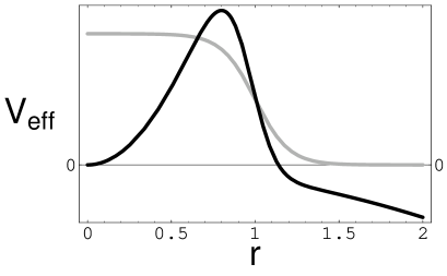
Figure 3: A schematic view of the effective potential $V_{eff}(r)$ for $L=0$. The gray curve indicates $\beta(r)$.

Now, we confront the question: why should we focus on the $L=0$ mode? One answer is the setting of $L=0$ seems most simple and probable. Another answer is that we might consider averaging the (“angular”) variables, such that

$$\frac{1}{2\pi}\int_{0}^{2\pi}\Psi(r,\phi)d\phi\propto\psi_{0}(r)\,.$$ (62)

Even in the classical noncommutative solutions, averaging yielded interesting results. Further discussions are provided in the last section.

VI Conclusion and discussion

In this work, we investigated classical and quantum solutions for a toy model of bicosmology. We considered a symmetric model with two scale factors. We then derived the classical equations for the model in the presence of noncommutativities both between the canonical momenta and between the dynamical variables of the minisuperspace. Further, we studied the system with the nonconstant noncommutativity in momenta for small scale factors and explored classical and quantum cosmological solutions. In this system, the tunneling wave function can be found, which may provide a new mechanism of the creation of the universe, even though the curvature of our space is zero.

We must comment on the aforementioned averaging of variables. According to the original idea put forward in Refs. FGMG ; FGGM ; FGM ; MM , two scale factors represent the causally disconnected regions. Naturally, it can be supposed that such two regions are extracted from a lot of typical regions in the universe. Considering the averaging is therefore not a very new procedure. However, the average presented here of the scale factors shows strange fractional powers (such as $x\propto a^{\frac{D-1}{2}}$), so expressing a proper averaging in terms of the classical metrics requires further consideration. When it comes to the wave function of the universe, averaging is a speculative but interesting conjecture, because it explains the creation of a finite-size flat universe.

An important problem is to find the mechanism for determining the critical value of $r_{c}$ (as well as the finite $\beta_{0}$). Unfortunately, this is a difficult problem with few clues at the moment.

A pressing problem, on the other hand, is to introduce the curvature of the space and matter fields into the model. We point out that introducing of phantom (scalar) fields Caldwell ; CKW ; DSS ; DKS ; KS into the model allows us to choose a well-defined boundary condition for the wave function at the origin of the minisuperspace without changing the signature of the minisuperspace metric, although there are various difficulties associated with phantom fields.

In addition, it is worth considering further cases with general noncommutative configuration variables (such as Sec. III) and other possibilities such as $[X,\Pi_{X}]=if(\Pi_{X},\Pi_{Y})$ (see Refs. BS ; SB for example), by classical and quantum approaches.

- (1) H. Falomir, J. Gamboa, F. Méndez and P. Gondolo, “Inflation without inflation: A model for dark energy”, Phys. Rev. D96 (2017) 083534. DOI: 10.1103/PhysRevD.96.083534 arXiv:1707.04670 [gr-qc].
- (2) H. Falomir, J. Gamboa, P. Gondolo and F. Méndez, “Magnetic seed and cosmology as quantum hall effect”, Phys. Lett. B785 (2018) 399. DOI: 10.1016/j.physletb.2018.08.055 arXiv:1801.07575 [hep-th].
- (3) H. Falomir, J. Gamboa and F. Méndez, “A noncommutative model of cosmology with two metrics”, Symmetry 12 (2020) 435. DOI: 10.3390/sym12030435 arXiv:1807.08359 [hep-th].
- (4) C. Maldonado and F. Méndez, “Bimetric universe with matter”, Phys. Rev. D103 (2021) 123505. DOI: 10.1103/PhysRevD.103.123505 arXiv:2103.11235 [gr-qc].
- (5) K. Aoki and K. Maeda, “Dark matter in ghost-free bigravity theory”, Phys. Rev. D90 (2014) 124089. DOI: 10.1103/PhysRevD.90.124089 arXiv:1409.0202 [gr-qc].
- (6) A. Schmidt-May and M. von Strauss, “Recent developments in bimetric theory”, J. Phys. A49 (2016) 183001. DOI: 10.1088/1751-8113/49/18/183001 arXiv:1512.00021 [hep-th].
- (7) F. Darabi and M. Mousavi, “Classical and quantum cosmology of minimal massive bigravity”, Phys. Lett. B761 (2016) 269. DOI: 10.1016/j.physletb.2016.08.031 arXiv:1512.03333 [gr-qc].
- (8) H. García-Compeán, O. Obregón and C. Ramírez, “Noncommutative quantum cosmology”, Phys. Rev. Lett. 88 (2002) 161301. DOI: 10.1103/PhysRevLett.88.161301 hep-th/0107250.
- (9) G. D. Barbosa and N. Pinto-Neto, “Noncommutative geometry and cosmology”, Phys. Rev. D70 (2004) 103512. DOI: 10.1103/PhysRevD.70.103512 hep-th/0407111.
- (10) L. O. Pimentel and C. Mora, “Noncommutative quantum cosmology”, Gen. Rel. Grav. 37 (2005) 817. DOI: 10.1007/s10714-005-0066-3 gr-qc/0408100.
- (11) L. O. Pimentel and O. Obregón, “Non commuting quantum cosmology with scalar matter”, Gen. Rel. Grav. 38 (2006) 553. DOI: 10.1007/s10714-006-0246-9
- (12) M. Aguero, J. A. S. Aguilar, C. Ortiz, M. Sabido and J. Socorro, “Noncommutative Bianchi type II quantum cosmology”, Int. J. Theor. Phys. 46 (2007) 2928. DOI: 10.1007/s10773-007-9405-3
- (13) W. Guzmán, M. Sabido and J. Socorro, “Noncommutativity and scalar field cosmology”, Phys. Rev. D76 (2007) 087302. DOI: 10.1103/PhysRevD.76.087302 arXiv:0712.1520 [gr-qc].
- (14) W. Guzmán, M. Sabido and J. Socorro, “Towards an inflationary scenario in noncommutative quantum cosmology”, Rev. Mex. Fís. 53 suppl. 4 (2007) 94.
- (15) W. Guzmán, M. Sabido and J. Socorro, “Towards noncommutative supersymmetric quantum cosmology”, AIP Conf. Proc. 1318 (2010) 209. DOI: 10.1063/1.3531633 arXiv:0812.4999 [hep-th].
- (16) E. Mena, O. Obregón and M. Sabido, “On the WKB approximation of noncommutative quantum cosmology”, Rev. Mex. Fís. 53 suppl. 4 (2007) 118.
- (17) E. Mena, O. Obregón and M. Sabido, “WKB-type approximation to noncommutative quantum cosmology”, Int. J. Mod. Phys. D18 (2009) 95. DOI: 10.1142/S0218271809014376 gr-qc/0701097.
- (18) C. Ortiz, E. Mena, M. Sabido and J. Socorro, “(Non)commutative isotropization in Bianchi I with barotropic perfect fluid and cosmological”, Int. J. Theor. Phys. 47 (2008) 1240. DOI: 10.1007/s10773-007-9557-1 gr-qc/0703101.
- (19) J. Socorro, L. O. Pimentel, C. Ortiz and M. Aguero, “Scalar field in the Bianchi I: Noncommutative classical and quantum cosmology”, Int. J. Theor. Phys. 48 (2009) 3567. DOI: 10.1007/s10773-009-0164-1 arXiv:0910.2449 [gr-qc].
- (20) C. Bastos, O. Bertolami, N. C. Dias and J. N. Prata, “Phase-space noncommutative quantum cosmology”, Phys. Rev. D78 (2008) 023516. DOI: 10.1103/PhysRevD.78.023516 arXiv:0712.4122 [gr-qc].
- (21) C. Bastos, O. Bertolami, N. C. Dias and J. N. Prata, “Noncommutative quantum cosmology”, J. Phys. Conf. Ser. 174 (2009) 012053. DOI: 10.1088/1742-6596/174/1/012053 arXiv:0812.3488 [gr-qc].
- (22) C. Bastos, O. Bertolami, N. Dias and J. N. Prata, “Noncommutative quantum mechanics and quantum cosmology”, Int. J. Mod. Phys. A24 (2009) 2741. DOI: 10.1142/S0217751X09046138 arXiv:0904.0400 [hep-th].
- (23) M. Maceda, A. Macías and L. O. Pimentel, “Homogeneous noncommutative quantum cosmology”, Phys. Rev. D78 (2008) 064041 DOI: 10.1103/PhysRevD.78.064041.
- (24) O. Obregón and I. Quiros, “Can noncommutative effects account for the present speed up of the cosmic expansion?”, Phys. Rev. D84 (2011) 044005. DOI: 10.1103/PhysRevD.84.044005 arXiv:1011.3896 [gr-qc].
- (25) S. M. M. Rasouli and P. V. Moniz, “Noncommutative minisuperspace, gravity-driven acceleration, and kinetic inflation”, Phys. Rev. D90 (2014) 083533. DOI: 10.1103/PhysRevD.90.083533 arXiv:1411.1346 [gr-qc].
- (26) S. M. M. Rasouli, A. H. Ziaie, S. Jalalzadeh and P. V. Moniz, “Non-singular Brans–Dicke collapse in deformed phase space”, Ann. Phys. (NY) 375 (2016) 154. DOI: 10.1016/j.aop.2016.09.007 arXiv:1608.05958 [gr-qc].
- (27) S. M. M. Rasouli and P. V. Moniz, “Gravity-driven acceleration and kinetic inflation in noncommutative Brans–Dicke setting”, Odessa Astron. Pub. 29 (2016) 19. DOI: 10.18524/1810-4215.2016.29.84956 arXiv:1611.00085 [gr-qc].
- (28) S. Jalalzadeh, A. J. S. Capistrano and P. V. Moniz, “Quantum deformation of quantum cosmology: A framework to discuss the cosmological constant problem”, Phys. Dark Univ. 18 (2017) 55. DOI: 10.1016/j.dark.2017.09.011 arXiv:1709.09923 [gr-qc].
- (29) S. M. M. Rasouli, N. Saba, M. Farhoudi, J. Marto and P. V. Moniz, “Inflationary universe in deformed phase space scenario”, Ann. Phys. (NY) 393 (2018) 288. DOI: 10.1016/j.aop.2018.04.014 arXiv:1804.03633 [gr-qc].
- (30) S. M. M. Rasouli, J. Marto and P. V. Moniz, “Kinetic inflation in deformed phase space Brans–Dicke cosmology”, Phys. Dark Univ. 24 (2019) 100269. DOI: 10.1016/j.dark.2019.100269 arXiv:1805.05978 [gr-qc].
- (31) N. Kan, M. Kuniyasu, K. Shiraishi and K. Takimoto, “Accelerating cosmologies in an integrable model with noncommutative minisuperspace variables”, J. Phys. Comm. 4 (2020) 075010. DOI: 10.1088/2399-6528/aba1d3 arXiv:1903.07895 [gr-qc].
- (32) S. Jalalzadeh, M. Rashki and S. abarghouei Nejad, “Classical universe arising from quantum cosmology”, Phys. Dark Universe 30 (2020) 100741. DOI: 10.1016/j.dark.2020.100741 arXiv:2001.00556 [gr-qc].
- (33) H. García-Compeán, O. Obregón and C. Ramírez, “Topics in supersymmetric and noncommutative quantum cosmology”, Universe 7 (2021) 434. DOI: 10.3390/universe7110434
- (34) S. M. M. Rasouli, “Noncommutativity, Sáez–Ballester theory and kinetic inflation”, Universe 8 (2022) 165. DOI: 10.3390/universe8030165 arXiv:2203.00765 [gr-qc].
- (35) E. Wigner, “On the quantum correction for thermodynamic equilibrium”, Phys. Rev. 40 (1932) 749. DOI: 10.1103/PhysRev.40.749.
- (36) W. B. Case, “Wigner functions and Weyl transforms for pedestrians”, Am. J. Phys. 76 (2008) 937. DOI: 10.1119/1.2957889.
- (37) J. Weinbub and D. K. Ferry, “Recent advances in Wigner function approaches”, App. Phys. Rev. 5 (2018) 041104. DOI: 10.1063/1.5046663.
- (38) E. Guendelman and D. Singleton, “Momentum gauge fields and non-commutative space-time”, arXiv:2206.02638 [quant-ph].
- (39) J. B. Hartle and S. W. Hawking, “Wave function of the universe”, Phys. Rev. D28 (1983) 2960. DOI: 10.1103/PhysRevD.28.2960
- (40) S. W. Hawking, “The quantum state of the universe”, Nucl. Phys. B239 (1984) 257. DOI: 10.1016/0550-3213(84)90093-2.
- (41) J. J. Halliwell, “Introductory lectures on quantum cosmology”, in Proceedings of the Jerusalem Winter School on Quantum Cosmology and Baby Universe (edited by T. Piran, World Scientific, Singapore, 1991), DOI: 10.1142/9789814503501_0003. arXiv:0909.2566 [gr-qc].
- (42) C. Kiefer, Quantum Gravity, Int. Ser. Monogr. Phys. Vol. 155 (Clarendon Press, Oxford, 2012). DOI: 10.1093/acprof:oso/9780199585205.001.0001
- (43) C. Kiefer, “Conceptual problems on quantum gravity and quantum cosmology”, ISRN Mathematical Physics 2013 (2013) 509316. DOI: 10.1155/2013/509316. arXiv:1401.3578 [gr-qc].
- (44) A. Boumali and Z. Selama, “Two-dimensional Klein–Gordon oscillator in the presence of a minimal length”, Phys. Part. Nuclei Lett. 15 (2018) 473. DOI: 10.1134/S1547477118050047 arXiv:1706.08593 [quant-ph].
- (45) Z. Selama and A. Boumali, “Two-dimensional boson oscillator under a magnetic field in the presence of a minimal length in the non-commutative space”, Rev. Mex. Fis. 67 (2021) 226. DOI: 10.31349/RevMexFis.67.226
- (46) R. R. Caldwell, “A phantom menace? cosmological consequences of a dark energy component with super-negative equation of state”, Phys. Lett. B545 (2002) 23. DOI: 10.1016/S0370-2693(02)02589-3 astro-ph/9908168.
- (47) R. R. Caldwell, M. Kamionkowski and N. N. Weinberg, “Phantom energy: Dark energy with causes a cosmic doomsday”, Phys. Rev. Lett. 91 (2003) 071301. DOI: 10.1103/PhysRevLett.91.071301 astro-ph/0302506.
- (48) M. P. Dabrowski, T. Stachowiak and M. Szydlowski, “Phantom cosmologies”, Phys. Rev. D68 (2003) 103519. DOI: 10.1103/PhysRevD.68.103519 hep-th/0307128.
- (49) M. P. Dabrowski, C. Kiefer and B. Sandhöfer, “Quantum phantom cosmology”, Phys. Rev. D74 (2006) 044022. DOI: 10.1103/PhysRevD.74.044022 hep-th/0605229.
- (50) D. E. Kaplan and R. Sundrum, “A symmetry for the cosmological constant”, JHEP 0607 (2006) 042. DOI: 10.1088/1126-6708/2006/07/042 hep-th/0505265.