Chirp-Based Over-the-Air Computation for Long-Range Federated Edge Learning

Abstract

In this study, we propose -based (CSC-MV), a power-efficient over-the-air computation (OAC) scheme, to achieve long-range federated edge learning (FEEL). The proposed approach maps the votes (i.e., the sign of the local gradients) from the edge devices to the linear CSCs constructed with a discrete Fourier transform-spread orthogonal frequency division multiplexing (DFT-s-OFDM) transmitter. At the edge server (ES), the MV is calculated with an energy detector. We compare our proposed scheme with one-bit broadband digital aggregation (OBDA) and show that the output-power back-off (OBO) requirement of the transmitters with an adjacent-channel-leakage ratio (ACLR) constraint for CSC-MV is lower than the one with OBDA. For example, with an ACLR constraint of $-22$ dB, CSC-MV can have an OBO requirement of $6-7$ dB less than the one with OBDA. When the power amplifier (PA) non-linearity is considered, we demonstrate that CSC-MV outperforms OBDA in terms of test accuracy for both homogeneous and heterogeneous data distributions, without using channel state information (CSI) at the ES and EDs.

I Introduction

FEEL is an implementation of federated learning (FL) over a wireless network, in which many EDs participate in training and an ES aggregates the local decisions without accessing the local data at the EDs [1]. With FEEL, a significant number of model parameters/gradients/updates needs to be exchanged between the ES and the EDs through a band-limited wireless channel. However, in this scenario, conventional orthogonal multiple access techniques can cause a large per-round communication latency as the number of EDs grows. One solution to this problem is to exploit the signal superposition property of wireless channels to compute the necessary calculations needed for the training over the air [2]. However, multipath fading, imperfect power control, and synchronization errors in a practical network can complicate the design of a reliable OAC scheme. Also, several wireless communication metrics such as ACLR, peak-to-mean envelope power ratio (PMEPR), cubic metric (CM), and PA efficiency need to be taken into account in practice as FEEL heavily relies on the uplink transmission and the availability of a large number of EDs such as low-cost Internet-of-Things (IoT) devices (e.g., battery-powered sensors) as in Long Range (LoRa) networks. In this paper, we propose an OAC method that particularly addresses the communication-related challenges of FEEL with CSC [3].

In the literature, OAC, which was initially considered for wireless sensor networks [4, 5], has recently been investigated for distributed learning over a wireless network with both digital and analog modulations. In [6], amplitude modulation over orthogonal frequency division multiplexing (OFDM) subcarriers, i.e., called broadband analog aggregation (BAA), with the model parameters is proposed. To overcome the impact of multi-path fading on the aggregation, truncated-channel inversion (TCI) is utilized, where the symbols on the OFDM subcarriers are multiplied by the inverse of the channel coefficients, and the fading subcarriers are not used. In [7], OBDA, where the signs of the gradients are mapped to the quadrature phase-shift keying (QPSK) symbols and transmitted along with TCI, is investigated. In [8], the authors analyze a scenario where the ES is equipped with multiple antennas and the CSI is not available to the EDs. To achieve coherent combining, the ES uses superposed CSIs. In [9], an OAC scheme based on sign stochastic gradient descent (signSGD) [10] with MV is proposed. This method does not rely on the CSI since it calculates the MV by comparing the energy accumulation over the orthogonal resources. Therefore, it is immune to time-synchronization errors. In the literature, there are few studies that consider the PMEPR for OAC. In [11], it is shown that if the gradients are correlated, the resulting OFDM symbol with OBDA can cause very high instantaneous peak power. To address this issue, the signs of the gradients are represented as PPM symbols constructed with DFT-s-OFDM. Nevertheless, PMEPR can still be high depending on the choice of the parameters, e.g., pulse duration in a PPM symbol.

In this work, we propose a new OAC approach based on CSCs, particularly tailored for scenarios where a power-efficient transmission is needed for FEEL to achieve wider coverage. Our specific contributions are listed as follows:

• By exploiting inherently low PMEPR of CSCs [3] and inspired by the simplicity of distributed training by the MV with signSGD [10], we show how to design chirp-based distributed learning over a wireless network. With the proposed scheme, we indicate the signs of local stochastic gradients by changing the positions of CSCs. We also do not use CSI at the EDs and ES.

• We show that the proposed scheme requires less OBO than that of OBDA for a given ACLR constraint. A reduced OBO results in increased cell coverage, which enables long-range distributed learning in a wireless network.

• We demonstrate the proposed approach can provide high test accuracy under both homogeneous and heterogeneous data distribution scenarios. We show that the proposed OAC scheme allows the model to learn the classes available at the cell-edge ED by increasing the cell size under a spectral leakage constraint.

Notation: The sets of complex and real numbers are denoted by $\mathbb{C}$ and $\mathbb{R}$, respectively. The function $\operatorname{sign}(\cdot)$ gives $1$ and $-1$ for a non-negative and a negative argument, respectively. The $N$-dimensional all zero and one vectors are $\textbf{{0}}_{N}$ and $\textbf{{I}}_{N}$, respectively. $\mathbb{I}\left[{\cdot}\right]$ denotes the indicator function.

II System Model

II-A Deployment

We consider a circular cell of radius $R_{\rm max}$ meters with an ES at its center. We assume that all the EDs are deployed uniformly at a radial distance from $R_{\rm min}$ meters to $R_{\rm max}$ meters from the ES. All EDs and ES are equipped with a single antenna. We consider time-synchronization errors while frequency synchronization is assumed to be perfect.

In this study, we consider a power control mechanism that considers the maximum transmit power constraint at the EDs. To model this, let $P_{\rm ref}/\sigma_{\rm n}^{2}$ be the signal-to-noise ratio (SNR) of an ED at the ES location when the corresponding link distance is $R_{\rm ref}$ meters. Without loss of generality, we consider $P_{\rm ref}=1$ W. We then express the received signal power of the $k$th ED located at the distance $r_{k}$ away from the ES as

$$P_{r_{k}}=\begin{cases}\left(\frac{{r_{k}}}{R_{\rm ref}}\right)^{-\alpha+\beta}P_{\rm ref},&0\leq r_{k}<r_{\rm P}\\ \left(\frac{{r_{\rm P}}}{R_{\rm ref}}\right)^{-\alpha+\beta}P_{\rm ref},&r_{k}\geq r_{\rm P}\end{cases}~{},$$ (1)

where $\alpha$ is the path loss exponent of the corresponding channel, $\beta\in[0,\alpha]$ is a coefficient that determines how much path loss is compensated, and $r_{\rm P}>R_{\rm ref}$ is the threshold distance beyond which the EDs are unable to attain the desired SNR at the ES. To determine $r_{\rm P}$, we consider the impact of PA non-linearity on the transmitted signals from EDs and set an ACLR constraint as follows: Let $\textrm{OBO}_{\rm{ref}}$ be the OBO for the link distance $R_{\rm ref}$ to achieve the desired SNR. Also, let $\textrm{OBO}_{\rm min}$ be the minimum OBO (i.e., results in maximum spectral tolerable growth) that fulfills the ACLR constraint. The path loss compensation can be maintained perfectly (i.e., $\beta=\alpha$) up to a range of $r_{\rm P}$. Thus, $P_{r_{k}}=1$ for $0\leq r_{k}<r_{\rm P}$. The transmitted signal power of the ED located at $r_{k}$ is $\left({{r_{k}}}/{R_{\rm ref}}\right)^{\beta}$ for $0\leq r_{k}<r_{\rm P}$. Let $P_{\rm max}$ be the maximum power output of the PA. Then, $\textrm{OBO}_{\rm{ref}}=10\log_{10}\left(P_{\rm max}\right/P_{\rm ref})$ and $\textrm{OBO}_{\rm min}=10\log_{10}\left(P_{\rm max}/P_{\rm ref}\left({R_{\rm ref}}/{{r_{\rm P}}}\right)^{\beta}\right)$, we then calculate $r_{\rm P}$ as

$$r_{\rm P}=R_{\rm ref}\times 10^{\frac{\textrm{OBO}_{\rm{ref}}-\textrm{OBO}_{\rm min}}{10\beta}}.$$ (2)

Therefore, for a signal with a lower PMEPR, $\textrm{OBO}_{\rm min}$ is a smaller value and the coverage is larger.

II-B Signal Model: Circularly-Shifted Chirps

In this work, we utilize the DFT-s-OFDM block to carry the gradient information with chirps by using the method introduced in [3]. In [3], it is shown that a chirp signal can be synthesized through DFT-s-OFDM with a special choice of frequency-domain spectral shaping (FDSS) coefficients with the motivation of its compatibility to 3GPP 4G LTE and 5G NR. In this study, we adopt this approach and the EDs access the spectrum with the CSCs synthesized through DFT-s-OFDM, simultaneously, given by

$$\textbf{{t}}_{k,m}=\textbf{{F}}_{N}^{\rm H}\textbf{{M}}_{\textrm{f}}{\rm diag}\{{\rm\bf f}\}\textbf{{D}}_{M}\textbf{{d}}_{k,m}^{(n)}~{},$$ (3)

where $\textbf{{t}}_{k,m}\in\mathbb{C}^{N}$ is the $m$th transmitted baseband signal in discrete time for the $k$th ED, $\textbf{{F}}_{N}^{\rm H}\in\mathbb{C}^{N\times N}$ is the orthonormal $N$-point inverse DFT (IDFT) matrix, $\textbf{{D}}_{M}\in\mathbb{C}^{M\times M}$ is the orthonormal $M$-point discrete Fourier transform (DFT) matrix, $\textbf{{M}}_{\textrm{f}}\in\mathbb{R}^{N\times M}$ is the mapping matrix that maps the output of the DFT precoder to a set of subcarriers, ${\rm\bf f}\in\mathbb{C}^{M}$ is the FDSS vector to synthesize chirps, and $\textbf{{d}}_{k,m}^{(n)}\in\mathbb{C}^{M}$ contains the symbols on $M$ bins. In [3], it is shown that $\textbf{{t}}_{k,m}$ is a linear combination of linear CSCs where the amount of frequency sweep for each CSC is $\frac{D}{T_{\rm s}}$ for symbol duration $T_{\rm s}$ if the vector ${\rm\bf f}$ is expressed as ${\rm\bf f}=[c_{L_{\rm d}},\dots,c_{L_{\rm u}}]^{\top}\times{\sqrt{M/{\sum_{j=L_{\rm d}}^{L_{\rm u}}{|c_{j}|^{2}}}}}$, where $c_{j}$ is given by

$$c_{j}=\gamma_{j}(C(\alpha_{j})+C(\beta_{j})+{\rm j}S(\alpha_{j})+{\rm j}S(\beta_{j}))~{}.$$ (4)

$C(\cdot)$ and $S(\cdot)$ are the Fresnel integrals with cosine and sine functions, respectively, $\alpha_{j}=(D/2+2\pi j)/\sqrt{\pi D}$, $\beta_{j}=(D/2-2\pi j)/\sqrt{\pi D}$, $\gamma_{j}=\sqrt{\frac{\pi}{D}}{\rm e}^{-{\rm j}\frac{(2\pi j)^{2}}{2D}-{\rm j}\pi j}$ for $j\in\{L_{\rm d},\hbox to10.00002pt{.\hss.\hss.},L_{\rm u}\}$, $L_{\rm d}\leq-D/2$, $L_{\rm u}\geq D/2$, and $L_{\rm u}-L_{\rm d}+1=M$. The spectrogram of a linear combination of two linear CSCs is depicted in Figure 1.

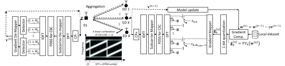
Figure 1: FEEL with CSC-MV. Due to its compatibility to 5G NR, DFT-s-OFDM with a special FDSS is utilized to generate multiple linear CSCs [3].

The cyclic prefix (CP) duration is assumed to be larger than the maximum-excess delays of the channels between the EDs and ES. Thus, the $m$th received baseband signal in discrete-time can be written as

$$\textbf{{r}}_{m}=\sum_{k=0}^{K-1}\sqrt{P_{r_{k}}}\textbf{{H}}_{k}\textbf{{t}}_{k,m}+\textbf{{n}}_{m}~{},$$ (5)

where $\textbf{{H}}_{k}\in\mathbb{C}^{N\times N}$ is a circular-convolution matrix based on the DFT of the channel impulse response (CIR) of the channels between EDs and ES, and $\textbf{{n}}_{m}\sim\mathcal{CN}(\textbf{{0}}_{N},\sigma_{\rm n}^{2}\textbf{{I}}_{N})$ is the additive white Gaussian noise (AWGN). At the ES, the aggregated symbols on the bins can be expressed as

$$\tilde{\textbf{{{d}}}}_{m}=\textbf{{D}}_{M}^{\rm H}\textbf{{M}}_{\textrm{f}}^{\rm H}{\rm diag}\{{{\rm\bf f}}^{\rm H}\}\textbf{{F}}_{N}\textbf{{r}}_{m}~{},$$ (6)

where $\tilde{\textbf{{{d}}}}_{m}\in\mathbb{C}^{M}$ are the received symbols on the bins.

II-C Learning Model

Let $\mathcal{D}$ be the dataset containing all the labeled data samples. Also, let the vectors x and ${y}$ be a data sample and its associated label, respectively for $\{({\textrm{{x}}},{y})\}\in\mathcal{D}$. Let $\mathcal{D}_{k}$ denote the local dataset for user index, $k=0,1,\dots,K-1$ such that $\mathcal{D}=\bigcup_{k=1}^{K}{\mathcal{D}_{k}}$. The centralized loss function can be expressed as

$$F(\textbf{w}) =\frac{1}{|\mathcal{D}|}\sum_{\forall({\textrm{{x}}},{y})\in\mathcal{D}}f(\textbf{w},{\textrm{{x}}},{y})$$

$$=\sum_{k=1}^{K}{\frac{1}{|\mathcal{D}_{k}|}\sum_{\forall({\textrm{{x}}},{y})\in\mathcal{D}_{k}}f(\textbf{w},{\textrm{{x}}},{y})}=\frac{1}{K}\sum_{k=1}^{K}{F_{k}(\textbf{w})}~{},$$ (7)

where $\textbf{w}=[{w}_{1},\hbox to10.00002pt{.\hss.\hss.},{w}_{q}]^{\rm T}\in\mathbb{R}^{q}$ is the parameter vector, $f(\textbf{w},{\textrm{{x}}},{y})$ denotes the sample loss function that measures the labeling error for $({\textrm{{x}}},{y})$. In the case of distributed learning, the goal is to minimize the loss function in (7) to find the desired parameter vector w, i.e.,

$$\textbf{w}^{*}=\arg\min_{\textbf{w}}{F(\textbf{w})}~{},$$ (8)

where the dataset are not uploaded to a centralized server.

To solve (8), the procedure for distributed training by the MV based on signSGD [10] can be summarized as follows: Let $\tilde{\textbf{g}}_{k}^{(n)}$ be the local stochastic gradient vector of the $k$th ED, given by

$$\tilde{\textbf{g}}_{k}^{(n)}=\nabla F_{k}(\textbf{w}^{(n)})=\frac{1}{n_{\rm b}}\sum_{\forall({\textrm{{x}}},{y})\in\mathcal{\tilde{D}}_{k}}\nabla f(\textbf{w}^{(n)},{\textrm{{x}}},{y})~{},$$ (9)

where $\mathcal{\tilde{D}}_{k}\subset\mathcal{D}_{k}$ is the set of the selected data samples and $n_{\rm b}=|\mathcal{\tilde{D}}_{k}|$ is the batch size, $\textbf{w}^{(n)}$ is the parameter vector at the $n$th communication round. Let ${\tilde{g}}_{k,i}^{(n)}$ be the $i$th element of $\tilde{\textbf{g}}_{k}^{(n)}$. All EDs calculate their votes as ${{\bar{g}}_{k,i}^{(n)}}\triangleq{\operatorname{sign}\left({\tilde{g}}_{k,i}^{(n)}\right)},\forall i,k$, and provide them to the ES. The ES then obtains the MV ${v}^{(n)}_{i}$ for the $i$th gradient with the expression given by

$${v}^{(n)}_{i}\triangleq\operatorname{sign}\left(\sum_{k=1}^{K}{\operatorname{sign}\left({\tilde{g}}_{k,i}^{(n)}\right)}\right)=\operatorname{sign}\left(\sum_{k=1}^{K}{{\bar{g}}_{k,i}^{(n)}}\right),\forall i~{}.$$ (10)

Afterwards, the ES sends the calculated MV vector $\textbf{v}^{(n)}\triangleq[{v}^{(n)}_{1},\hbox to10.00002pt{.\hss.\hss.},{v}^{(n)}_{q}]^{\rm T}$ to the EDs. All the EDs update their parameters for the next communication round as

$$\textbf{w}^{(n+1)}=\textbf{w}^{(n)}-\eta\textbf{v}^{(n)}~{},$$ (11)

where $\eta$ is the learning rate.

In this study, we consider the same procedure outlined above. However, we consider its implementation in a wireless network and calculate the MV in (10) with an OAC scheme that relies on CSCs.

III CSC-Based Majority Vote

In this section, we discuss the transmitter at EDs and the receiver ES with the proposed OAC scheme. We also elaborate on the convergence rate of the distributed learning when the proposed OAC is used for the MV calculation.

III-A Edge Device - Transmitter

We encode the gradients with CSCs as follows: Let $S$ be the number of blocks used in the transmission to train the model for each communication round. Each block can synthesize $M$ CSCs corresponding to the $M$ DFT-s-OFDM bins. From the $MS$ available indices, we propose to assign two active indices for the $i$ th gradient. In this case, the number of votes that can be carried for each block is equal to $M_{\rm v}=\left\lfloor{M}/{(2+2M_{\rm g})}\right\rfloor$. To express the mapping rigorously, let ${f}$ be a pre-defined function that maps $i\in\{1,2,\hbox to10.00002pt{.\hss.\hss.},q\}$ to the distinct pairs $(m^{+},l^{+})$ and $(m^{-},l^{-})$ for $m^{+},m^{-}\in\{0,1,\hbox to10.00002pt{.\hss.\hss.},S-1\}$ and $l^{+},l^{-}\in\{0,1,\hbox to10.00002pt{.\hss.\hss.},2M_{\rm v}-1\}$. Let $(\textbf{{d}}_{k,{m}}^{(n)})_{j}$ be the symbol at the $j$th index of the $m$th symbol for the $k$th user. For all $i$, we then set the corresponding symbols as

$$(\textbf{{d}}_{k,{m^{+}}}^{(n)})_{l^{+}(1+M_{\rm g})}=s_{k,i}\mathbb{I}\left[{{\bar{g}}_{k,i}^{(n)}=1}\right]~{},$$ (12)

and

$$(\textbf{{d}}_{k,{m^{-}}}^{(n)})_{l^{-}(1+M_{\rm g})}=s_{k,i}\mathbb{I}\left[{{\bar{g}}_{k,i}^{(n)}=-1}\right]~{},$$ (13)

where $s_{k,i}$ is a random symbol on the unit circle to introduce randomness to the synthesized symbols and $M_{\rm g}\geq 0$ is a parameter to set the guard period between the CSCs. Due to the channel dispersion, delay spread, and potential time synchronization errors, the CSCs can interfere with each other. We deactivate $M_{\rm g}$ indices followed by any active index to avoid interference. The inactivated indices provide a guard period of $T_{\rm g}=M_{\rm g}T_{\rm s}/M$ between two adjacent CSCs. Let the delay due to time-synchronization error be $T_{\rm sync}$ seconds and the maximum delay of the channel be $T_{\rm chn}$ seconds. Hence, the negligible interference can be ensured by choosing $M_{\rm g}$ under the condition given by

$$T_{\rm g}=\frac{M_{\rm g}T_{\rm s}}{M}\geq T_{\rm chn}+T_{\rm sync}~{}.$$ (14)

III-B Edge Server - Receiver

The mapping function ${f}$ is assumed to be known to the ES so that the ES can calculate the pairs $(m^{+},l^{+})$ and $(m^{-},l^{-})$ for a given $i$. The MV for the $i$th gradient can be obtained as

$${v}^{(n)}_{i}=\operatorname{sign}\left({\Delta}^{(n)}_{i}\right)~{},$$ (15)

where ${\Delta}^{(n)}_{i}\triangleq{r_{i}^{+}-r_{i}^{-}}$ for $r_{i}^{+}\triangleq\sum_{j=l^{+}(1+M_{\rm g})}^{(l^{+}+1)(1+M_{\rm g})-1}{|{(\tilde{\textbf{{{d}}}}_{m^{+}})_{j}}|^{2}}$ and $r_{i}^{-}\triangleq\sum_{j=l^{-}(1+M_{\rm g})}^{(l^{-}+1)(1+M_{\rm g})-1}{|{(\tilde{\textbf{{{d}}}}_{m^{-}})_{j}}|^{2}}$. We consider $(1+M_{\rm g})$ bins for the energy calculations for $r_{i}^{+}$ and $r_{i}^{-}$. The transmitter and the receiver block diagrams are provided in Figure 1.

III-C Convergence Rate

The MV computed with (15) obtains the original MV given in (10), probabilistically, due to the non-coherent detection. Nevertheless, for a non-convex loss function $F(\textbf{w})$, we can show that CSC-MV still maintains the convergence of the original MV in [10] under the assumptions given as follows:

Assumption 1 (Bounded loss function).

$\forall\textbf{w}$, $\exists F^{*}$ such that $F(\textbf{w})\geq F^{*}$.

Assumption 2 ($L$-smooth gradient [12]).

Let g be the gradient of $F(\textbf{w})$ evaluated at w. $\forall\textbf{w}$ and $\forall\textbf{w}^{\prime}$, the expression given by

$$\left|F(\textbf{w}^{\prime})-(F(\textbf{w})-{\textbf{{g}}}^{\rm T}(\textbf{w}^{\prime}-\textbf{w}))\right|\leq\frac{1}{2}\sum_{i=1}^{q}L_{i}({w}_{i}^{\prime}-{w}_{i})^{2}~{},$$

holds for some vector with non-negative constant values, i.e., $\textbf{L}=[L_{1},\hbox to10.00002pt{.\hss.\hss.},L_{q}]^{\rm T}$.

Assumption 3 (Bounded variance).

The local estimates of the stochastic gradient, $\{\tilde{\textbf{g}}_{k}=[{\tilde{g}}_{k,1},\hbox to10.00002pt{.\hss.\hss.},{\tilde{g}}_{k,q}]^{\rm T}=\nabla F_{k}(\textbf{w}^{(n)})\}$, $\forall k$, are independent and unbiased estimates of ${\textbf{{g}}}=[{g_{1}},\hbox to10.00002pt{.\hss.\hss.},{g_{q}}]^{\rm T}=\nabla F(\textbf{w})$ with a coordinate bounded variance, i.e., ${\mathbb{E}}\left[\tilde{\textbf{g}}_{k}\right]={\textbf{{g}}},~{}\forall k$ and ${\mathbb{E}}\left[({\tilde{g}}_{k,i}-{g_{i}})^{2}\right]\leq\sigma_{i}^{2}/n_{\rm b},~{}\forall k,i$, where ${\bm{\sigma}}=[\sigma_{1},\hbox to10.00002pt{.\hss.\hss.},\sigma_{q}]^{\rm T}$ is a non-negative constant vector.

Assumption 4 (Unimodal, symmetric gradient noise).

For a given w, each element of the vector $\tilde{\textbf{g}}_{k}$, $\forall k$, follows a unimodal distribution that is symmetric around its mean.

We assume that CSCs are orthogonal to each other. This assumption is not strong because the interference among them can be maintained negligibly low under (14). Hence, by using the steps mentioned in [11], based on the aforementioned assumptions, the following theorem can be derived:

Theorem 1.

For $n_{\rm b}=N/\gamma$ and $\eta=1/\sqrt{\lVert\textbf{L}\rVert_{1}n_{\rm b}}$, the convergence rate of CSC-MV based FEEL in fading channel can be expressed as,

$${\mathbb{E}}\left[\frac{1}{N}\sum_{n=0}^{N-1}\lVert{\textbf{{g}}}^{(n)}\rVert_{1}\right]\leq\frac{1}{\sqrt{N}} \bigg{(}a\sqrt{\lVert\textbf{L}\rVert_{1}}\left(F(\textbf{w}^{(0)})-F^{*}+\frac{\gamma}{2}\right)$$

$$~{}~{}+\frac{2\sqrt{2\gamma}}{3}\lVert{\bm{\sigma}}\rVert_{1}\bigg{)}~{},$$ (16)

where $a=(1+\frac{2}{\xi K})\frac{1}{\sqrt{\gamma}}$ for $\xi\triangleq\frac{E_{\rm s}}{(1+M_{\rm g})\sigma_{\rm n}^{2}}$.

III-D Trade-offs and Comparisons

The schemes in [6, 7, 8] rely on OFDM modulation. However, OFDM is known to suffer from high PMEPR. The main advantage of CSC-MV is that it can achieve a significantly low PMEPR compared to the methods in [6, 7, 8, 11]. The scheme in [11] is also based on DFT-s-OFDM leading to low PMEPR symbols. However, theoretically, CSC-MV can decrease the PMEPR even further and can achieve a PMEPR as low as $0~{}$dB (for $M_{\rm v}=1$), unlike the method in [11]. For our scheme, the PMEPR increases with the number of chirps [13]. Hence, for $M_{\rm v}$ votes, the PMEPR is $10\log_{10}{M_{\rm v}}$. The number of symbols needed to train each round is $\lceil\frac{q}{M_{\rm v}}\rceil{}$. Thus, CSC-MV causes a trade-off between PMEPR and resource consumption. As a result, we must increase the PMEPR limit to reduce resource utilization.

OBDA [7] and BAA [6] rely on the CSI being available to the EDs. Although the proposed scheme in [8] does not require the CSI to be available on the EDs, the ES utilizes multiple antennas to overcome the impact of fading, and the sum of the channel gains from the ED to each antenna is assumed to be available to the ES. CSC-MV does not rely on the summed CSI or multiple antennas. Non-coherent detection also aids in the elimination of synchronization issues as it does not need phase synchronization.

Finally, the methods in [6] and [8] rely on analog transmission, which is incompatible with the existing digital modulation-based wireless systems. Similar to OBDA [7], CSC-MV is compatible with digital modulation. Also, since the proposed scheme synthesizes CSC over DFT-s-OFDM, it is compatible with the transceivers in 5G NR.

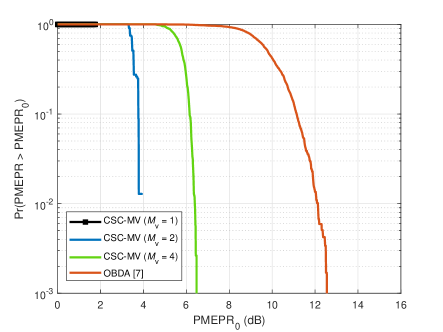
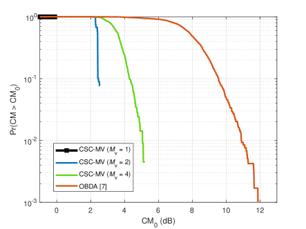
Figure 2: PMEPR distributions.

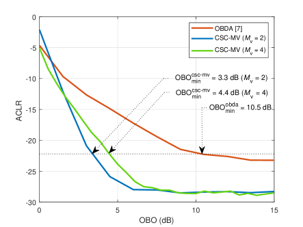
Figure 3: CM distributions.

Figure 4: ACLR versus OBO plot for different schemes.

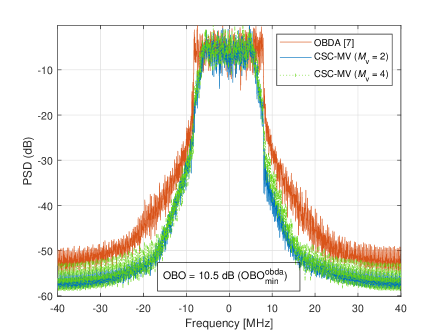
(a) Operating at $\textrm{OBO}=10.5$ dB.

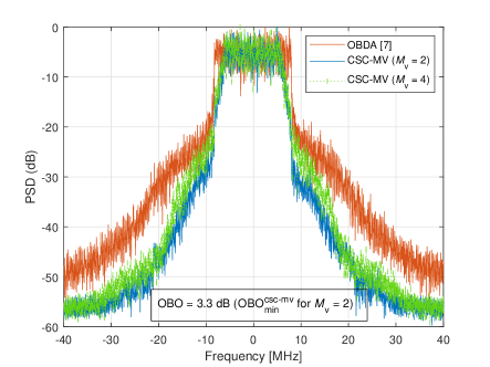
(b) Operating at $\textrm{OBO}=3.3$ dB.

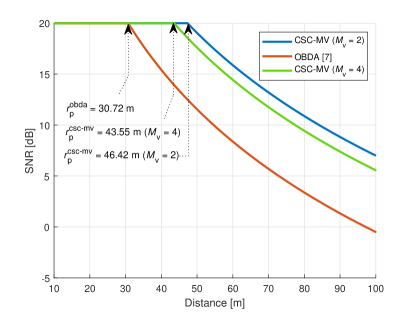
Figure 5: OOB performance of CSC-MV and OBDA at different OBO levels.

Figure 6: SNR versus link distance performance for $\textrm{OBO}_{\rm{ref}}=30$ dB.

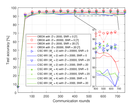
Figure 7: Test accuracy results for homogeneous data distributions.

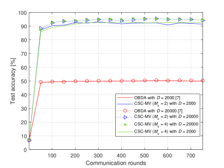
(a) SNR is $0$ dB.

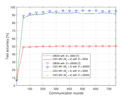
(b) SNR is $20$ dB.

Figure 8: Average test accuracy results for heterogeneous data distributions (EPA, $N=750$, $K=50$).

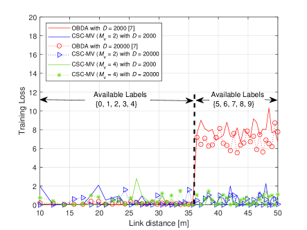
(a) SNR is $0$ dB.

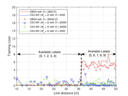
(b) SNR is $20$ dB.

Figure 9: Training loss versus link distance results for heterogeneous data distributions after 750 communication round (EPA, $K=50$).

IV Numerical Results

We consider the learning task of handwritten digit recognition over a FEEL system in a circular cell with a radius of $R_{\rm max}=50$ m and the number of EDs, $K=50$. The path loss exponent is $\alpha=4$. We assume perfect power control within the coverage range (i.e., ${r_{k}}<r_{\rm P}{}$) and $\textrm{OBO}_{\rm{ref}}$ is set to $30$ dB, and $R_{\rm ref}=R_{\rm min}=10$ m. We consider the Rapp model for the PA at the EDs with the saturation amplitude of $1$ and the smoothness factor of $3$. We compare the performance of CSC-MV with OBDA in this setup for both homogeneous and heterogeneous data distributions. For homogeneous data distribution, all digits are equally assigned to each ED. For heterogeneous data distributions, the cell is divided into two equal areas with an equal number of EDs. The first area is the circle with a radius of $R_{\rm max}/\sqrt{2}$. The second area is the ring-shaped area enclosed by two concentric circles with radius $R_{\rm max}/\sqrt{2}$ and $R_{\rm max}$. The EDs located at the first and the second area only have the data samples with labels $\{0,1,2,3,4\}$ and $\{5,6,7,8,9\}$, respectively (See [9, Figure 3] for illustration).

Our model is based on the convolution neural network (CNN) given in [9], which contains $q=123090$ learnable parameters. We considered $M=54$ subcarriers and IDFT size $N=64$. The FEEL performance is tested under two different uplink SNRs, i.e., $0$ dB and $20$ dB. ITU Extended Pedestrian A (EPA) is considered for the fading channel with no mobility for each round and the channel variation is considered by regenerating the channel at each communication round. The root-mean-square (RMS) delay spread of the EPA channel is $T_{\rm rms}=43.1$ ns. For each round, we transmit $61545$ and $30773$ symbols for $M_{\rm v}=2$ and $M_{\rm v}=4$, respectively.

In Figure 4, the PMEPR distributions are compared. The OBDA can cause substantially high PMEPR as the signs of the gradients may result in a constructive addition in the time domain. The CSCs, on the other hand, result in low PMEPR as shown in III-D. When $M_{\rm v}$ is $1$, $2$, or $4$, The PMEPR is approximately $2$ dB, $3$ dB, and $6$ dB, respectively. However, theoretically, the PMEPR should be $0$ dB, $2$ dB, and $4$ dB when $M_{\rm v}$ is $1$, $2$, or $4$, respectively. The synthesized signal is distorted due to the abrupt frequency change of the linear CSCs within a symbol duration[3]. As a result, the observed PMEPR is larger than the theoretical bound. However, PMEPR can be improved by choosing very small $D$ or by modifying the FDSS vector ${\rm\bf f}$ [3].

The CM distributions are shown in Figure 4. The CM of a time-domain signal $x(t)$ is calculated as ${\rm CM}(x(t))=({{\rm RCM}_{x(t)}-{\rm RCM}_{\rm ref}})/{K_{\rm s}}$, where the empirical slope factor $K_{\rm s}$ is set to $1.52$ for OFDM systems and ${\rm RCM}_{x(t)}$ is defined by ${\rm RCM}_{x(t)}=20\log_{10}\left(x_{\rm norm}(t){}\right)$, where $x_{\rm norm}(t)$ is the normalized signal. For the reference signal, we set ${\rm RCM}_{\rm ref}$ to be $1.52$ dB[14]. For $M_{\rm v}=1$, Figure 4 demonstrates that CSC-MV performs even better than the reference signal. Similar to the PMEPR results, CSC-MV outperforms OBDA for $M_{\rm v}\in\{1,2,4\}$.

Figure 4 shows the ACLR versus OBO plot for CSC-MV and OBDA. For both schemes, we consider a time-domain windowing with a raised cosine window to minimize spectral leakage. We define ACLR as the ratio of the power received outside the allocated frequency band of the channel to the received power on the assigned channel bandwidth. The plots show that under similar ACLR constraints, the power amplifier must operate at a larger OBO value for the OBDA compared to the CSC-MV. Moreover, the lowest ACLR that OBDA and CSC-MV can achieve is $-23$ dB and $-28.22$ dB, respectively. If we consider an ACLR constraint of $-22$ dB, we calculate $\textrm{OBO}_{\rm min}^{\rm obda}=10.5$ dB, $\textrm{OBO}_{\rm min}^{\rm csc\textrm{-}mv}=3.3$ dB for $M_{\rm v}=2$ and $\textrm{OBO}_{\rm min}^{\rm csc\textrm{-}mv}=4.4$ dB for $M_{\rm v}=4$ as the minimum OBO values at the PAs for the corresponding schemes. Figure 6LABEL:sub@subfig:oobchirp and Figure 6LABEL:sub@subfig:oobobda show the OOB performance for different schemes at $\textrm{OBO}=\textrm{OBO}_{\rm min}^{\rm csc\textrm{-}mv}$ and $\textrm{OBO}=\textrm{OBO}_{\rm min}^{\rm obda}$, respectively. The plots show that the OBDA is more prone to the spectral leakage problem than CSC-MV. In Figure 6, the uplink SNR versus link distance performances are shown under the ACLR constraint. The curves indicate that the power control can maintain the uplink SNR up to a range of $r_{\rm P}$, where the range of power control for OBDA, CSC-MV ($M_{\rm v}=2$) and CSC-MV ($M_{\rm v}=4$) are $30.72$ m, $43.55$ m, and $46.42$ m, respectively. Hence, the area of the cell is appropriately doubled with $M_{\rm v}=2$ as compared to OBDA.

Figure 7 shows the test accuracy results for homogeneous data distribution for $\acs{SNR}=\{0,20\}$ dB, $K=50$, and $D=\{2000,20000\}$. Both OBDA and CSC-MV perform with high accuracy in all scenarios. We define all the EDs at $R\leq r_{\rm P}$ as near EDs and the ones at $R>r_{\rm P}$ as far EDs. For the given setup, the number of near EDs for OBDA, CSC-MV ($M_{\rm v}=2$) and CSC-MV ($M_{\rm v}=4$) are 20, 37, and 42, respectively. For OBDA, the votes of the 20 near EDs have a stronger impact compared to the random votes of the 30 far EDs that are affected by the imperfect power control. The training remains unaffected and OBDA performs well for homogeneous data distributions.

Figure 9 shows that CSC-MV performs much better than OBDA in terms of test accuracy for heterogeneous data distributions. Although Assumption 3 does not hold in the case of heterogeneous data distribution, the test results are still remarkable for CSC-MV. The test accuracy results can be further understood from the loss vs. link-distance performance after 750 iterations given in Figure 9. For OBDA, the plot shows that the 20 near EDs only have half of the available labels. As a result, the trained model fails to distinguish the other half of the digits and the test accuracy is near $50\%$, i.e., the learning is biased towards the nearby EDs. For CSC-MV ($M_{\rm v}=4$), of the 37 near EDs, 25 of them have the dataset with labels $\{0,1,2,3,4,\}$, and the remaining 12 EDs have the dataset with labels $\{5,6,7,8,9\}$. The availability of all the labels allows the model to converge with high test accuracy. For the same reason, the test accuracy is high for CSC-MV ($M_{\rm v}=2$).

V Concluding Remarks

In this study, we propose a CSC-based OAC for FEEL. To implement FEEL, all the design challenges for a practical wireless communication system (e.g., PMEPR, CM, spectral leakage) must be taken into account. The main advantage of CSC-MV is the improved power efficiency with low distortion, which results in larger cell size as compared to OBDA under an ACLR constraint. Also, CSC-MV can work at a much lower OBO level than the one for OBDA. For a distributed learning scenario, a better PA efficiency is crucial for reducing the cost of the devices that operate with a low link budget, e.g., IoT sensors. On the other hand, CSC-MV requires a larger number of symbols as compared to OBDA. We demonstrate that a larger cell size helps to achieve a high test accuracy for heterogeneous data distributions, particularly, when the dataset changes based on the location of the devices. Numerical results show that, compared to OBDA, CSC-MV leads to a larger area in which ED can converge, resulting in high test accuracy. In the future, the proposed concept will be enhanced to decrease the number of symbols transmitted while maintaining the power-efficiency.

References

- [1] T. Gafni, N. Shlezinger, K. Cohen, Y. C. Eldar, and H. V. Poor, “Federated learning: A signal processing perspective,” 2021. [Online]. Available: arXiv:2103.17150
- [2] M. Chen, D. Gündüz, K. Huang, W. Saad, M. Bennis, A. V. Feljan, and H. V. Poor, “Distributed learning in wireless networks: Recent progress and future challenges,” 2021. [Online]. Available: arXiv:2104.02151
- [3] A. Sahin, N. Hosseini, H. Jamal, S. S. M. Hoque, and D. W. Matolak, “DFT-Spread-OFDM-based chirp transmission,” IEEE Communications Letters, vol. 25, no. 3, pp. 902–906, 2021.
- [4] M. Goldenbaum, H. Boche, and S. Stańczak, “Harnessing interference for analog function computation in wireless sensor networks,” IEEE Trans. Signal Process., vol. 61, no. 20, pp. 4893–4906, Oct. 2013.
- [5] B. Nazer and M. Gastpar, “Computation over multiple-access channels,” IEEE Trans. Inf. Theory, vol. 53, no. 10, pp. 3498–3516, Oct. 2007.
- [6] G. Zhu, Y. Wang, and K. Huang, “Broadband analog aggregation for low-latency federated edge learning,” IEEE Trans. Wireless Commun., vol. 19, no. 1, pp. 491–506, Jan. 2020.
- [7] G. Zhu, Y. Du, D. Gündüz, and K. Huang, “One-bit over-the-air aggregation for communication-efficient federated edge learning: Design and convergence analysis,” IEEE Trans. Wireless Commun., vol. 20, no. 3, pp. 2120–2135, Nov. 2021.
- [8] M. M. Amiri, T. M. Duman, D. Gündüz, S. R. Kulkarni, and H. V. Poor, “Blind federated edge learning,” IEEE Trans. Wireless Commun., vol. 20, no. 8, pp. 5129–5143, 2021.
- [9] A. Şahin, B. Everette, and S. Hoque, “Distributed learning over a wireless network with FSK-based majority vote,” in Proc. IEEE International Conference on Advanced Communication Technologies and Networking (CommNet), Dec. 2021, pp. 1–9.
- [10] J. Bernstein, Y.-X. Wang, K. Azizzadenesheli, and A. Anandkumar, “signSGD: Compressed optimisation for non-convex problems,” in Proc. in International Conference on Machine Learning, vol. 80. Proceedings of Machine Learning Research, 10–15 Jul 2018, pp. 560–569.
- [11] A. Şahin, B. Everette, and S. Hoque, “Over-the-air computation with DFT-spread OFDM for federated edge learning,” in Proc. IEEE Wireless Communications and Networking Conf. (WCNC), Apr. 2022, pp. 1–6.
- [12] Y. Nesterov, Introductory Lectures on Convex Optimization: A Basic Course. Kluwer Academic Publishers, 2004.
- [13] S. Hoque, C.-Y. Chen, and A. Şahin, “A wideband index modulation with circularly-shifted chirps,” in Proc. IEEE Consumer Commun. & Netw. Conf. (CCNC), Jan. 2021, pp. 1–6.
- [14] 3GPP TSG-RAN WG1 LTE, Motorola, “Cubic Metric in 3GPP LTE,” R1-060023, Tech. Rep., Jan. 2006.