An Algebra of Observables for de Sitter Space

Abstract

We describe an algebra of observables for a static patch in de Sitter space, with operators gravitationally dressed to the worldline of an observer. The algebra is a von Neumann algebra of Type II₁. There is a natural notion of entropy for a state of such an algebra. There is a maximum entropy state, which corresponds to empty de Sitter space, and the entropy of any semiclassical state of the Type II₁ algebras agrees, up to an additive constant independent of the state, with the expected generalized entropy $S_{\mathrm{gen}}=(A/4G_{N})+S_{\mathrm{out}}$. An arbitrary additive constant is present because of the renormalization that is involved in defining entropy for a Type II₁ algebra.

1 Introduction

1.1 Background

Not long after it was understood that an entropy should be associated to the horizon area of a black hole Bekenstein ; Hawking , Gibbons and Hawking GH proposed that similarly, the area of a cosmological horizon should be interpreted as an entropy. Specifically, they considered an observer in a de Sitter space with radius of curvature $r_{\mathrm{dS}}$. The worldline of the observer is assumed to be timelike. The region of de Sitter space that is causally accessible to such an observer is bounded by past and future horizons. Gibbons and Hawking associated to the horizon of an observer an entropy $A/4G_{N}$ (where $A$ is the area of the observer’s horizon and $G_{N}$ is Newton’s constant) and a temperature $T_{\mathrm{dS}}=1/2\pi r_{\mathrm{dS}}=1/\beta_{\mathrm{dS}}$. The temperature, but not the entropy, had been defined earlier by Figari, Hoegh-Krohn, and Nappi FHN .

A difference between a black hole horizon and a cosmological horizon is that, in a sense, the notion of a cosmological horizon is more observer-dependent. A black hole horizon in an asymptotically flat (or asymptotically Anti de Sitter) spacetime is defined in terms of the region that is causally accessible to any observer at infinity. In a cosmological model such as de Sitter space, different observers can see and can influence different parts of the spacetime, and experience different horizons. De Sitter space has a great deal of symmetry, such that the horizon of any observer has the same area. That is not true in a more general cosmological model.

It seems fair to say that although black hole entropy remains highly enigmatic to this day, the entropy of a cosmological horizon, such as the de Sitter horizon, is only more mysterious. A working hypothesis, expressed in a modern form in Review , is that black hole entropy measures the logarithm of the dimension of a quantum Hilbert space that is needed to describe a black hole as seen by an observer who remains outside the horizon. What would be the analog of this for cosmological horizons? A plausible analog of an observer who remains outside the black hole horizon is an observer in de Sitter space whose horizon is under discussion. The region of de Sitter space causally accessible to such an observer has been called a “static patch.” Thus a possible analog of the working hypothesis about black hole entropy would be to say that the de Sitter entropy measures the logarithm of the dimension of the quantum Hilbert space that an observer in the static patch can use to account for inaccessible degrees of freedom beyond the horizon.

Something somewhat along these lines has actually been proposed BoussoOne ; BoussoTwo ; Banks ; BanksFischler ; BanksOne ; BanksTwo ; BFTwo ; SusskindA ; Susskind , but with a subtle difference. To explain this point, let us consider a de Sitter space that instead of being empty, as considered originally by Gibbons and Hawking, contains ordinary particles and fields and perhaps even some small black holes. In this case, we follow Bekenstein and define a generalized entropy that includes the horizon entropy $A/4G_{N}$ and also the ordinary entropy $S_{\mathrm{out}}$ of the matter that the observer can see:

$$S_{\mathrm{gen}}=\frac{A}{4G_{N}}+S_{\mathrm{out}}.$$ (1)

In the case of a black hole in an asymptotically flat spacetime, both terms $A/4G_{N}$ and $S_{\mathrm{out}}$ can be arbitrarily large, and it takes an infinite-dimensional Hilbert space to describe the possible states of the world as seen by an outside observer. In the case of de Sitter space, it has been argued that this is not the case: it is claimed that the maximum possible value for $S_{\mathrm{gen}}$ is the value that it has for empty de Sitter space Maede ; BoussoOne ; BoussoTwo . One can certainly increase $S_{\mathrm{out}}$ by considering a state in which the static patch is not empty. The claim is that this has the effect of reducing the horizon area, in such a way that the decrease in $A/4G_{N}$ exceeds the increase in $S_{\mathrm{out}}$.

The proposal, then, is that empty de Sitter space maximizes the entropy of any state of the static patch. Here by empty de Sitter space we mean the generalization with gravity included of the natural de Sitter invariant state of quantum fields in de Sitter space CT ; SS ; BD ; Mo ; Al , which is often called the Bunch-Davies state. Thus in leading order for small $G_{N}$, the maximum possible entropy of a state of the static patch, including particles and fields and black holes it may contain and also degrees of freedom that are somehow associated to the cosmological horizon, is $A_{\mathrm{dS}}/4G_{N}$, where $A_{\mathrm{dS}}$ is the horizon area of empty de Sitter space. (For the one-loop correction to the formula $A_{\mathrm{dS}}/4G_{N}$ for the entropy of empty de Sitter space, see Denef .)

The existence of a maximum entropy state of de Sitter space makes possible an interpretation of de Sitter entropy that does not quite have an analog for black hole entropy. The proposal is that a Hilbert space of dimension roughly $\exp(A_{\mathrm{dS}}/4G_{N})$ suffices to describe all possible states of the static patch, including any matter and black holes it may contain and also the cosmological horizon BoussoOne ; BoussoTwo ; Banks ; BanksFischler ; BanksOne ; BanksTwo ; BFTwo ; SusskindA ; Susskind . Empty de Sitter space would then be described by the maximally mixed state on this finite-dimensional Hilbert space DST ; SusskindB . By contrast, in the case of a black hole, the Bekenstein-Hawking entropy $A/4G_{N}$ possibly determines the size of a Hilbert space that describes the black hole as seen from outside, but this Hilbert space does not describe particles and fields outside the black hole horizon.

The claim that empty de Sitter space is maximally mixed may sound counterintuitive, since the Bunch-Davies state of quantum fields reduces on the static patch to a thermal ensemble with temperature $T_{{\mathrm{dS}}}$. The idea is that this thermal distribution comes purely from entropic, rather than energetic, suppression on the full static-patch Hilbert space BanksTwo ; BanksOne ; Susskind . As a simple illustration, consider a particle with energy $E$ at rest in the center of the static patch. The presence of such a particle reduces the area of the cosmological horizon from $A_{\mathrm{dS}}$ to

$$A_{\mathrm{hor}}/4G=A_{{\mathrm{dS}}}/4G-\beta_{{\mathrm{dS}}}E.$$ (2)

We will recall the derivation of this statement in section 3. If the total number of microstates is $\exp(A_{\mathrm{dS}}/4G)$, and the number of microstates such that the particle has energy $E$ is $\exp(A_{\mathrm{hor}}/4G)$, then assuming that each microstate is equiprobable, the probability to observe a particle of energy $E$ in the center of the static patch will be

$$p(E)=\exp(-\beta_{dS}E).$$ (3)

In this way, one can obtain a thermal distribution purely on entropic grounds.

1.2 A Type II₁ Algebra For The Static Patch

In the present article, we will make a contribution to the understanding of de Sitter entropy by defining a von Neumann algebra of Type II₁ that, in the limit of small $G_{N}$, describes the possible observations of an observer in de Sitter space. We will also reconsider and generalize a previous discussion in which, inspired by considerations involving the large $N$ limit in holography LL ; LLtwo , observations outside a black hole horizon were described by an algebra of Type II_∞ GCP .

The entanglement entropy of a local region in quantum field theory is always ultraviolet divergent, as discovered long ago Sorkin ; BKLS . An abstract explanation of why this happens is that the algebra of observables in a local region in quantum field theory is of Type III Araki , and there is no notion of entropy for a state of an algebra of Type III. By contrast, for states of an algebra of Type II, it is possible to define an entropy, though in physical terms this is a sort of renormalized entropy with a state-independent divergent constant subtracted. Thus, at least for the black hole and de Sitter space, the fact that gravity converts the algebra of observables from being of Type III to being of Type II gives an abstract explanation of why the entropy of a region of spacetime is better-defined in the presence of gravity.

A Type II₁ algebra has a state of maximum entropy, as has been explained long ago Segal and reconsidered recently LongoWitten . Hence a Type II₁ algebra is a candidate for describing the physics of a static patch in de Sitter space, with empty de Sitter space corresponding to the state of maximum entropy. By contrast, there is no upper bound on the entropy of a state of a Type II_∞ algebra. Therefore, a Type II_∞ algebra is a candidate for describing physics outside the black hole horizon.

In section 2, we consider the problem of defining, in the limit $G_{N}\to 0$, an algebra of observables in a static patch of de Sitter space. There is no asymptotic region at infinity to which a local operator can be “gravitationally dressed,” so we assume the existence of an observer in the static patch and we gravitationally dress operators in the static patch to the worldline of the observer. We consider a minimal model in which the observer consists only of a clock. The resulting algebra is of Type II₁. The maximum entropy state of the Type II₁ algebra is the natural state of empty de Sitter space (tensored with a simple state of the observer). The density matrix of the maximum entropy state is the identity, in keeping with the idea that this state is maximally mixed and has a flat entanglement spectrum DST .

In section 3, we assume that the de Sitter space is not necessarily empty and show that (up to an additive constant that is independent of the state) the entropy of a semiclassical state of the Type II₁ algebra agrees with the generalized entropy $S_{\mathrm{gen}}=A/4G_{N}+S_{\mathrm{out}}$. In this, we closely follow an analysis we present elsewhere for the case of the Type II_∞ algebra of a black hole CPW . We also make use of a formula of Wall expressing the generalized entropy in terms of relative entropy on the horizon Wall .

An observer in a static patch in de Sitter space has access to observables that are localized in that patch, but has no way to know what there is beyond the horizon and therefore has no knowledge of a global quantum state of the whole system. However, with some assumptions about what is beyond the horizon, one can construct a global Hilbert space for the whole system, and the Type II₁ algebra constructed in section 2 should act naturally on this Hilbert space. We explore this question in section 4. We get a simple answer if we assume the existence behind the horizon of a second observer who is completely or almost completely entangled with the observer in the static patch. In the absence of such a second observer, the question is more difficult and appears not to have a simple limit for $G_{N}\to 0$.

Finally, in section 5 we reconsider the Type II_∞ algebra of the black hole. We define this Type II_∞ algebra in a way that makes sense for a black hole in an asymptotically flat spacetime (as opposed to the asymptotically AdS spacetime considered in GCP ). We also formulate the derivation in a way that shows a close analogy between the definition of the Type II_∞ algebra for the black hole and the Type II₁ algebra for de Sitter space.

Appendix A is an explanation of the crossed product construction for operator algebras and of Takesaki duality, which underlies the construction of the Type II₁ algebra for de Sitter space. In Appendix B, we explain how, in the presence of gravity, the symmetries of de Sitter space can be imposed as constraints in the construction of a Hilbert space of quantum states. Here we follow previous analysis higuchi ; marolf , the only novelty being to present the construction in the BRST framework; it is known in general that this is possible shvedov . We also explain why it is more straightforward to impose constraints on operators than on states. Some facts explained in the appendix are important background to this article, though we explain more than we strictly need.

1.3 What is a Type II₁ Algebra?

In the remainder of this introduction, we provide a short introduction to Type II₁ algebras.

A Type II₁ algebra is just the natural algebra of observables that acts on a countably infinite set of qubits in a state that is almost maximally mixed. In more detail, consider a system $A$ consisting of a countably infinite set of qubits that are almost completely entangled with an identical system $B$ also consisting of a countably infinite set of qubits. In the case of a finite number $N$ of qubit pairs, a state in which the $n^{th}$ qubit of system $A$ is maximally entangled with the $n^{th}$ qubit of system $B$ for all $n$ is

$$\Psi_{{\mathrm{TFD}}}=\frac{1}{2^{N/2}}\bigotimes_{n=1}^{N}\sum_{i=1,2}|i\rangle_{n,A}\otimes|i\rangle_{n,B}.$$ (4)

We have called this state $\Psi_{\mathrm{TFD}}$ because it can be viewed as the usual thermofield double state specialized to the case that the Hamiltonian is $H=0$. In the limit $N\to\infty$, one constructs a Hilbert space ${\mathcal{H}}_{\mathrm{TFD}}$ with the property that for any state in this space, almost all of the qubit pairs are almost completely entangled in the same way as in $\Psi_{\mathrm{TFD}}$. Let ${\sf a}$ be any operator that acts on only the first $k$ qubits of system $A$ and define

$$F({\sf a})=\langle\Psi_{\mathrm{TFD}}|{\sf a}|\Psi_{\mathrm{TFD}}\rangle.$$ (5)

Since $\Psi_{\mathrm{TFD}}$ has been chosen so that the qubits of the $A$ system are maximally mixed, the density matrix of the $A$ system is $\rho_{A}=2^{-N}\,I$, where $I$ is the identity matrix. So

$$F({\sf a})={\mathrm{Tr}}\,\rho_{A}{\sf a}=2^{-N}{\mathrm{Tr}}\,{\sf a},$$ (6)

and therefore, if ${\sf a},{\sf a}^{\prime}$ are two operators that both act only on the first $N$ qubits of system $A$, then

$$F({\sf a}{\sf a}^{\prime})=F({\sf a}^{\prime}{\sf a})=2^{-N}\,{\mathrm{Tr}}\,{\sf a}{\sf a}^{\prime}.$$ (7)

Some other important properties of $F({\sf a})$ are that it is normalized to

$$F(1)=1$$ (8)

and that it is positive, in the sense that

$$F({\sf a}^{\dagger}{\sf a})>0,~{}~{}{\sf a}\not=0.$$ (9)

The function $F({\sf a})$ is defined as soon as one includes all the qubits that ${\sf a}$ acts on in the definition of $\Psi_{\mathrm{TFD}}$, and it is unaffected by including additional qubits, so it is well-defined in the limit of an infinite system. Eqn. (7) says that the function $F({\sf a})$ has the algebraic property of a trace, and it is in fact convenient to denote it as one:

$$F({\sf a})={\mathrm{Tr}}\,{\sf a}.$$ (10)

Clearly then

$${\mathrm{Tr}}\,1=1$$ (11)

and

$${\mathrm{Tr}}\,{\sf a}^{\dagger}{\sf a}>0,~{}~{}{\sf a}\not=0.$$ (12)

So far we have defined the trace for the algebra ${\mathcal{A}}_{0}$ of all operators that act on only finitely many qubits of system $A$. However, the definition can be extended to a larger algebra ${\mathcal{A}}$ that consists of all operators that can be approximated sufficiently well by operators that act on only finitely many qubits of system $A$. (Technically, ${\mathcal{A}}$ contains operators that are weak limits of sequences of operators in ${\mathcal{A}}_{0}$.) The algebra ${\mathcal{A}}$ is known as a von Neumann algebra of Type II₁. The center of ${\mathcal{A}}$ consists only of complex scalars. In von Neumann algebra language, this means that ${\mathcal{A}}$ is a “factor,” somewhat analogous to a simple Lie group.

We are quite familiar with a more elementary example of an infinite algebra that has a trace, namely the algebra ${\mathcal{B}}$ of all (bounded) operators on a Hilbert space ${\mathcal{H}}$ of countably infinite dimension. This algebra has a trace, but it is not defined for all elements, only for those that are “trace class”; in particular, in the algebra ${\mathcal{B}}$, the trace of the identity operator is $+\infty$. By contrast, a Type II₁ algebra has a trace that is defined for all elements, and which can be normalized so that ${\mathrm{Tr}}\,1=1$. We will see that it is natural to define a Type II₁ algebra associated to de Sitter space. The tensor product of the two algebras ${\mathcal{A}}$ and ${\mathcal{B}}$ that we have described so far is an algebra ${\mathcal{C}}={\mathcal{A}}\otimes{\mathcal{B}}$ that turns out to be a von Neumann algebra of Type II_∞. ${\mathcal{C}}$ is a factor, since ${\mathcal{A}}$ and ${\mathcal{B}}$ are, and it has a trace, since ${\mathcal{A}}$ and ${\mathcal{B}}$ do, but the trace is not defined for all elements of ${\mathcal{C}}$, since that is the case for ${\mathcal{B}}$. In an asymptotic expansion near $N=\infty$, the algebra of observables outside a black hole horizon is of Type II_∞ GCP . This was found by incorporating some $1/N$ corrections in a construction of emergent Type III algebras in holographic duality LL ; LLtwo . Our main result in the present article is an analogous statement involving the static patch of de Sitter space and an algebra of Type II₁.

Though not the main focus of the present article, Type III von Neumann algebras can be constructed in a similar way, starting with the thermofield double state for a nonzero Hamiltonian. The Hamiltonian can be taken to be a simple sum of single qubit Hamiltonians, $H=\sum_{i}H_{i}$, where $H_{i}$ acts only on the $i^{th}$ qubit. In the thermodynamic limit, another novel algebra, now of Type III, can be defined just as before. The main difference is that this algebra does not have a trace. See for example Curved for a fuller explanation.

A Type II or Type III von Neumann algebra does not have an irreducible representation in a Hilbert space. Whenever such an algebra acts on a Hilbert space ${\mathcal{H}}$, it commutes with another algebra ${\mathcal{A}}^{\prime}$ that is also of the same type, Type II or Type III. For example, in the Murray-von Neumann construction of the Type II₁ factor ${\mathcal{A}}$ that we have just described, ${\mathcal{A}}$ obviously commutes with an isomorphic algebra $\widetilde{\mathcal{A}}$ that acts on system $B$. If $\Lambda$ is a projection operator in $\widetilde{\mathcal{A}}$, then $\Lambda{\mathcal{H}}$ is a subspace of ${\mathcal{H}}$ on which ${\mathcal{A}}$ acts. This motivates the question of how “small” $\Lambda$ can be and how much we can shrink ${\mathcal{H}}$ while still getting a Hilbert space on which ${\mathcal{A}}$ acts. This question was addressed by Murray and von Neumann. Projection operators $\Lambda$ in a Type II₁ algebra ${\mathcal{A}}$ (or $\widetilde{\mathcal{A}}$) are classified, up to unitary equivalence in the algebra, by their trace, and any value of the trace between 0 and 1 is possible. (The values 0 and 1 occur only for $\Lambda=0$ and $\Lambda=1$.) In the construction of ${\mathcal{A}}$ from the infinite system of entangled qubits, for any positive integers $k$ and $n$, the projection operator onto a $k$-dimensional subspace of the $2^{n}$-dimensional Hilbert space of the first $n$ qubits of system $A$ gives, in the large $N$ limit, a projection operator $\Lambda\in{\mathcal{A}}$ with ${\mathrm{Tr}}\,\Lambda=k/2^{n}$. By taking limits, one can define a projection operator $\Lambda\in{\mathcal{A}}$ with any trace between 0 and 1. (In section 4.2, we will find another construction of a projection operator in ${\mathcal{A}}$ with any desired value of the trace between 0 and 1.)

Murray and von Neumann showed that the Hilbert space representations of the algebra ${\mathcal{A}}$ are classified by a parameter $d$, called the continuous dimension, that can be any positive real number or $\infty$. The Hilbert space ${\mathcal{H}}_{\mathrm{TFD}}$ is defined to have $d=1$, and if $\Lambda\in\widetilde{\mathcal{A}}$ is a projection operator with ${\mathrm{Tr}}\,\Lambda=f$, then $\Lambda{\mathcal{H}}$ has $d=f$. Finally, $d$ is additive in direct sums, so for example the direct sum of $k$ copies of ${\mathcal{H}}_{\mathrm{TFD}}$ has $d=k$. By taking $d$ very small, we can make a “small” representation of ${\mathcal{A}}$, but there is no irreducible representation; any representation can always be reduced further. The “trace” function ${\mathrm{Tr}}\,{\sf a}$ that we defined earlier has the algebraic properties of a trace, but it is not actually the trace in any representation of ${\mathcal{A}}$; it is more like a trace with an infinite factor $\left.2^{N}\right|_{N\to\infty}$ removed.

Since an algebra of Type II₁ does not have an irreducible Hilbert space representation, there is no notion of a pure state of such an algebra. However, there is a notion of density matrices and entropies. This results from the fact that the bilinear form ${\mathrm{Tr}}\,{\sf a}{\sf a}^{\prime}$ on a pair of elements ${\sf a},{\sf a}^{\prime}\in{\mathcal{A}}$ is nondegenerate (the nondegeneracy is a consequence of the fact that ${\mathrm{Tr}}\,{\sf a}^{\dagger}{\sf a}>0$ for ${\sf a}\not=0$). So any linear function $F({\sf a})$ on the algebra is of the form ${\mathrm{Tr}}\,{\sf a}{\sf a}^{\prime}$ for a unique ${\sf a}^{\prime}\in{\mathcal{A}}$.

For example, if ${\mathcal{A}}$ acts on a Hilbert space ${\mathcal{H}}$ and $\Psi$ is a vector in ${\mathcal{H}}$, the function $F({\sf a})=\langle\Psi|{\sf a}|\Psi\rangle$ is a linear function on ${\mathcal{A}}$, so there is a unique $\rho\in{\mathcal{A}}$ such that

$$\langle\Psi|{\sf a}|\Psi\rangle={\mathrm{Tr}}\,{\sf a}\rho.$$ (13)

Since $\langle\Psi|{\sf a}^{\dagger}{\sf a}|\Psi\rangle\geq 0$ for all ${\sf a}\in{\mathcal{A}}$, we have ${\mathrm{Tr}}\,{\sf a}^{\dagger}{\sf a}\rho\geq 0$ for all ${\sf a}$. This is described by saying that $\rho$ is positive. Assuming that the state $\Psi$ is normalized to $\langle\Psi|\Psi\rangle=1$, we have ${\mathrm{Tr}}\,\rho=1$. So $\rho$ is a positive element of ${\mathcal{A}}$ of trace 1. By analogy with the standard terminology in ordinary quantum mechanics, such an element of ${\mathcal{A}}$ is called a density matrix, and we define $\rho$ to be the density matrix of the state $\Psi$, for observations in ${\mathcal{A}}$. As a simple example, consider the state $\Psi_{\mathrm{TFD}}$. Since by definition $\langle\Psi_{\mathrm{TFD}}|{\sf a}|\Psi_{\mathrm{TFD}}\rangle={\mathrm{Tr}}\,{\sf a}$, the density matrix of $\Psi_{\mathrm{TFD}}$ is $\rho=1$.

Conversely, suppose that we are given a density matrix $\rho\in{\mathcal{A}}$. In ordinary quantum mechanics, every density matrix has a (highly non-unique) “purification.” This statement has an analog for an algebra ${\mathcal{A}}$ of Type II₁. A purification of a density matrix $\rho\in{\mathcal{A}}$ is a Hilbert space ${\mathcal{H}}$ with an action of ${\mathcal{A}}$ and a state $\Psi\in{\mathcal{H}}$ such that ${\mathrm{Tr}}\,{\sf a}\rho=\langle\Psi|{\sf a}|\Psi\rangle$ for all ${\sf a}\in{\mathcal{A}}$. The GNS construction of operator algebra theory (see for example section 3.1 of Curved ) gives a simple construction of a purification of any state of a Type II₁ algebra, generalizing a standard construction in ordinary quantum mechanics in which a purification is constructed by doubling the Hilbert space.

Once one has density matrices, one can also define entropies; for example, the von Neumann entropy is defined as usual as

$$S(\rho)=-{\mathrm{Tr}}\,\rho\log\rho.$$ (14)

Rényi entropies are defined similarly:

$$S_{\alpha}(\rho)=\frac{1}{1-\alpha}\log{\mathrm{Tr}}\,\rho^{\alpha}.$$ (15)

These entropies have slightly unusual properties that we will discuss first informally and then in a more formal way.

The maximally mixed state of $N$ qubits has von Neumann entropy $N$. So the state $\Psi_{\mathrm{TFD}}$ on $N$ qubits, reduced to system $A$, has entropy $N$, and in the $N\to\infty$ limit its entropy diverges. A state obtained from $\Psi_{\mathrm{TFD}}$ by disentangling, say, $k$ qubits has entropy $N-k$, less than $N$ but also divergent for $N\to\infty$. To define entropies for a state in $\Psi_{\mathrm{TFD}}$, reduced to system $A$, we subtract $N$ before taking the large $N$ limit. With this definition, the maximally mixed state of the infinite system of qubits has entropy 0 and other states have negative entropy. This is the usual definition for states of an algebra of Type II₁. In short, entropy in a Type II₁ algebra is a renormalized entropy. There is a state of maximum entropy, whose entropy is defined to be 0, and other states have negative entropy.

Now let us see these properties from the definition $S(\rho)=-{\mathrm{Tr}}\,\rho\log\rho$. First of all, the state of maximum entropy is $\Psi_{\mathrm{TFD}}$, corresponding to $\rho=1$. For $\rho=1$, we do indeed have $S(\rho)=0$. To show that any other density matrix $\sigma$ has $S(\sigma)<0$, one way is as follows. In general let $\rho$ and $\sigma\not=\rho$ be two density matrices. As in ordinary quantum mechanics, one can interpolate between $\sigma$ and $\rho$ by the one-parameter family of density matrices $\rho_{t}=(1-t)\rho+t\sigma$, $0\leq t\leq 1$. Let $f(t)=S(\rho_{t})$. The same calculation as in ordinary quantum mechanics shows that $f^{\prime\prime}(t)\leq 0$ for $0\leq t\leq 1$. In other words, the entropy is concave. If $\rho=1$, one finds $f(0)=f^{\prime}(0)=0$, $f^{\prime\prime}(0)=-{\mathrm{Tr}}\,(1-\sigma)^{2}<0$. Therefore $f(t)<0$ for $0<t\leq 1$. In particular $S(\sigma)=f(1)<0$.

As an example that will be relevant in section 2, let $\Lambda$ be a nonzero projection operator in $\widetilde{\mathcal{A}}$. As explained earlier, its trace is a positive number that is no greater than 1 (and equal to 1 only if $\Lambda=1$). Therefore $\rho_{\Lambda}=\Lambda/{\mathrm{Tr}}\,\Lambda$ is a density matrix. To evaluate $S(\rho_{\Lambda})$, we note that the operator $\rho_{\Lambda}$ has the two eigenvalues 0 and $1/{\mathrm{Tr}}\,\Lambda$, so $\rho_{\Lambda}\log\rho_{\Lambda}=\rho_{\Lambda}\log(1/{\mathrm{Tr}}\Lambda)$ and hence $S(\rho_{\Lambda})=-{\mathrm{Tr}}\,\rho_{\Lambda}\log\rho_{\Lambda}=-\log(1/{\mathrm{Tr}}\,\Lambda)<0$.

The algebra of operators in a local region in ordinary quantum field theory is a von Neumann algebra of Type III, a statement that is more or less equivalent to the statement that neither pure states nor density matrices nor entropies can be defined for such an algebra. The main observation of the present article is that, provided an observer is included in the description of the static patch, gravity converts the Type III algebra of the static patch in de Sitter space to an algebra of Type II₁.

2 The Algebra Of The Static Patch

2.1 The Static Patch

What can be seen by an observer in de Sitter space? We will discuss this question first in the context of ordinary quantum field theory in a fixed de Sitter background, and then in the context of semiclassical quantization of gravity.

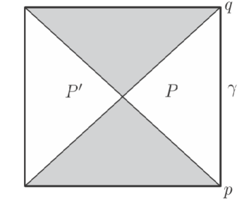
Figure 1: The Penrose diagram of de Sitter space. An observer enters at the point $p$ at past infinity and exits at the point $q$ at future infinity. Coordinates can be chosen to put these points at corners of the diagram, as shown. The observer’s worldline is a timelike curve $\gamma$ from $p$ to $q$, such as the geodesic from $p$ to $q$, shown here as the vertical line on the right boundary of the diagram. $P$ is the static patch of this observer, and $P^{\prime}$ is the complementary static patch, spacelike separated from $P$. The shaded regions are behind past and future horizons for an observer in either $P$ or $P^{\prime}$.

Imagine an observer who enters a $D$-dimensional de Sitter space $X$ at a point $p$ in past infinity and exits in the far future at a point $q$ in future infinity (fig. 1). From $p$ to $q$, the observer travels on some worldline $\gamma$. The part of de Sitter space that is causally accessible to the observer – the part that the observer can influence and can also see, or in other words the intersection of the past and future of $\gamma$ – is bounded by past and future horizons. The causally accessible region, which we will call $P$, is known as the static patch of the observer. $P$ depends only on the points $p$ and $q$ and not on the path $\gamma$. The region of $X$ that is spacelike separated from $P$, so that the observer can neither see nor influence it, is a complementary static patch $P^{\prime}$.

Consider first an ordinary quantum field theory on $X$, without gravity. Such a theory has a Hilbert space ${\mathcal{H}}$ of physical states. In general, in quantum field theory, the algebra of observables in any local region is a von Neumann algebra of Type III Araki . So in particular, the algebra of observables in the region $P$ is a Type III algebra ${\mathcal{A}}$ of operators on ${\mathcal{H}}$, and the algebra of observables in $P^{\prime}$ is a second Type III algebra ${\mathcal{A}}^{\prime}$, the commutant of the first (${\mathcal{A}}^{\prime}$ consists of the bounded operators that commute with ${\mathcal{A}}$, and vice-versa). The Type III nature of ${\mathcal{A}}$ and ${\mathcal{A}}^{\prime}$ means that there is no natural notion of entropy for a state of either of these algebras. Concretely, if one picks a state $\Psi\in{\mathcal{H}}$ and attempts to compute the entropy of the state $\Psi$ reduced to a region of spacetime, one will encounter an ultraviolet divergence, as first observed long ago Sorkin ; BKLS .

2.2 The Thermal Nature of de Sitter Space

The Hilbert space ${\mathcal{H}}$ of a quantum field theory in a fixed de Sitter background contains a distinguished state $\Psi_{\mathrm{dS}}$ CT ; SS ; BD ; Mo ; Al , sometimes called the Bunch-Davies state. The Euclidean version of de Sitter space is a sphere $S^{D}$, and the state $\Psi_{\mathrm{dS}}$ can be defined by analytic continuation from $S^{D}$. $\Psi_{\mathrm{dS}}$ is the natural “vacuum” of a quantum field in a background de Sitter space; it is the analog for de Sitter space of the Hartle-Hawking state of a black hole. $\Psi_{\mathrm{dS}}$ is invariant under the full automorphism group $G_{\mathrm{dS}}$ of de Sitter space, which is ${\mathrm{SO}}(1,D)$ or a double cover of this to include spin.

Once we choose to focus on a particular static patch $P$, what is relevant is not the full de Sitter automorphism group, but the subgroup $G_{P}$ that consists of automorphisms of $P$. Concretely, this subgroup is $G_{P}\cong{\mathbb{R}}\times{\mathrm{SO}}(D-1)$, where the first factor, which we will denote as ${\mathbb{R}}_{t}$, generates what we will call the time translations of the static patch. If the trajectory $\gamma$ of the observer is chosen to be the geodesic from $p$ to $q$, then ${\mathbb{R}}_{t}$ is the group of translations along $\gamma$, and the second factor in $G_{P}$, namely ${\mathrm{SO}}(D-1)$, is the group of rotations around $\gamma$. ${\mathbb{R}}_{t}$ is generated by a Killing vector field $V$ that we can choose to be future-directed timelike in the static patch $P$ and past-directed timelike in the complementary patch $P^{\prime}$. In ordinary quantum field theory in a fixed de Sitter background, ${\mathbb{R}}_{t}$ is generated by a conserved charge $H$ that acts on the Hilbert space ${\mathcal{H}}$.

As argued by Gibbons and Hawking GH (for earlier work see FHN ), in quantum field theory in a fixed de Sitter background, the state $\Psi_{\mathrm{dS}}$ has a thermal interpretation. The thermal interpretation arises because, after analytic continuation to Euclidean signature, $V$ becomes the generator of a rotation of $S^{D}$. As a result, correlation functions in the state $\Psi_{\mathrm{dS}}$ can be analytically continued to periodic functions in imaginary time and can be interpreted as correlation functions in a thermal ensemble with a Hamiltonian $H_{P}$ and inverse temperature $\beta_{\mathrm{dS}}=2\pi r_{\mathrm{dS}}$. Here $H_{P}$ generates time translations of the static patch and $r_{\mathrm{dS}}$ is the radius of curvature of the de Sitter space.

Importantly, $H_{P}$ is not the conserved charge $H$ associated to the Killing vector field $V$ of de Sitter space; the operator $H$ has no positivity, since $V$ is past-directed in the complementary patch $P^{\prime}$. Rather, $H_{P}$ is supposed to be a “one-sided” Hamiltonian that generates time translations in $P$, and does nothing in $P^{\prime}$. Because of fluctuations near the cosmological horizon – that is, near the boundary of $P$ – such an operator actually cannot be defined in the natural Hilbert space ${\mathcal{H}}$ of de Sitter space. However, it is possible with a sort of “brick wall” boundary condition on the cosmological horizon to define a Hilbert space ${\mathcal{H}}_{P}$ that describes excitations in region $P$ only and on which $H_{P}$ can be defined and is bounded below. Correlation functions in the state $\Psi_{\mathrm{dS}}\in{\mathcal{H}}$ of operators in the patch $P$ can be interpreted as thermal correlation functions of the same operators for a thermal density matrix on ${\mathcal{H}}_{P}$ that is proportional to $\exp(-\beta_{\mathrm{dS}}H_{P})$. This is one way to make precise the statement that correlation functions in the state $\Psi_{\mathrm{dS}}$ have a thermal interpretation.

All of this is in close analogy with the thermal nature of the Hartle-Hawking state of a black hole HH ; I and of the Minkowski space vacuum as seen by an accelerated observer Unruh . A more or less equivalent statement in the language of operator algebras is that, in the case of quantum field theory in a fixed de Sitter background, the “modular Hamiltonian” $H_{\mathrm{mod}}$ which generates the modular automorphism group of the algebra ${\mathcal{A}}$ of the static patch for the state $\Psi_{\mathrm{dS}}$ is

$$H_{\mathrm{mod}}=\beta_{\mathrm{dS}}H,$$ (16)

where $H$ generates time translations of the static patch. The analogous statement for the Rindler wedge, with the Minkowski space vacuum playing the role of $\Psi_{\mathrm{dS}}$, is due to Bisognano and Wichman BW ; this result was carried over to black holes by Sewell Sewell , and the de Sitter case is similar. The interpretation of $\beta_{\mathrm{dS}}H$ as the generator of the modular automorphism group will be very important in what we say later.

What has been described so far applies to quantum field theory in a fixed de Sitter background, without dynamical gravity. However, a number of authors BanksOne ; BanksTwo ; SusskindA ; Susskind have claimed in various ways that this picture is substantially modified when gravity becomes dynamical, even for very small values of Newton’s constant $G_{N}$. Without repeating all of the arguments here, we can motivate some of the claims as follows. In gravity, because diffeomorphisms are gauged, conserved charges associated to diffeomorphisms of spacetime can be computed as surface terms. In the case of a black hole in asymptotically flat or asymptotically AdS spacetime, the energy is an important conserved charge, and it can be measured as a surface term at spatial infinity, namely the ADM energy. However, the static patch in de Sitter space has no boundary at infinity. Its only boundary is the cosmological horizon. Therefore, gravity will force the time generator $H_{P}$ of the static patch to have an interpretation as a boundary term on the cosmological horizon. The leading boundary term when the de Sitter radius is large is the area of the cosmological horizon. But according to Gibbons and Hawking, this area is an approximation to the entropy of the static patch. So “energy” in the static patch is really entropy. One argument in this direction Susskind involves comparing the energy of a fluctuation in the static patch to the entropy reduction associated to observing that fluctuation. A quite different line of argument DST that leads to a somewhat similar conclusion involves use of a replica trick to argue that the state $\Psi_{\mathrm{dS}}$ has a flat entanglement spectrum (so that there is no relevant notion of “energy” independent of entropy). We will recover these claims by a simple but slightly abstract analysis of the operator algebra of the theory.

2.3 The Algebra of Observables

What algebra of observables is accessible to an observer in the static patch? A first thought might be that in ordinary quantum field theory, the observer can measure the quantum fields only in the immediate vicinity of the observer’s worldline $\gamma$. However, according to the Timelike Tube Theorem Borchers ; ArakiTwo , the algebra of observables in ordinary quantum field theory in an arbitrarily small neighborhood of $\gamma$ is the same as the algebra of observables in the static patch. Thus, in ordinary quantum field theory, it is reasonable to claim that the observer can access the whole algebra ${\mathcal{A}}$ of observables in $P$.

Now let us suppose that gravity is one of the fields that we want to consider in de Sitter space. We assume, however, that $G_{N}$ is extremely small, or to be more precise that the Planck length $\ell$ is much less than $r_{\mathrm{dS}}$. Then gravity is very weakly coupled and can be treated perturbatively. In leading order, we make a quadratic approximation to the gravitational action and quantize gravitational perturbations in de Sitter space in a free field approximation. This leads to the construction of a Hilbert space ${\mathcal{H}}_{\mathrm{grav}}$ that describes gravitational fluctuations. This must be included as a tensor factor in defining the Hilbert space ${\mathcal{H}}$ that was the input in the previous discussion. Thus the full Hilbert space, at this level, is

$${\mathcal{H}}={\mathcal{H}}_{\mathrm{matt}}\otimes{\mathcal{H}}_{\mathrm{grav}},$$ (17)

where now ${\mathcal{H}}_{\mathrm{matt}}$ is the Hilbert space obtained by quantizing the matter fields.

Including the weakly coupled gravitational field as one more quantum field in the construction of the Hilbert space does not qualitatively change anything what we have said so far about the algebra of observables. The Type III algebra ${\mathcal{A}}$ of the static patch now includes operators that act on the gravitational fluctuations just as they act on any other fluctuations. The extended Hilbert space still contains a natural state $\Psi_{\mathrm{dS}}$ that can be defined by analytic continuation from Euclidean signature and it still has a thermal interpretation.

What does qualitatively change the picture is that, as de Sitter space is a closed universe, with compact spatial sections, the automorphisms of de Sitter space have to be treated as gauge constraints. This means, in particular, that the Hilbert space that describes quantum fields and gravity in de Sitter space, in the limit $G_{N}\to 0$, is not ${\mathcal{H}}$ but rather is a Hilbert space $\widehat{\mathcal{H}}$ that is constructed from ${\mathcal{H}}$ by imposing the de Sitter generators as constraints. The procedure to do so is subtle. Naively, one might think that $\widehat{\mathcal{H}}$ would be the $G_{\mathrm{dS}}$-invariant subspace of ${\mathcal{H}}$, but this subspace is much too small, because, with the exception of $\Psi_{\mathrm{dS}}$, $G_{\mathrm{dS}}$-invariant states are not normalizable. Instead, $\widehat{\mathcal{H}}$ should be defined as a space of coinvariants higuchi ; marolf . Equivalently, as we explain in Appendix B, one can introduce a BRST complex for the action of $G_{\mathrm{dS}}$ on ${\mathcal{H}}$ and define $\widehat{\mathcal{H}}$ as the top degree BRST cohomology. The invariant subspace is the bottom degree BRST cohomology.

Our goal, however, is to describe not the physics of the whole de Sitter space $X$, but rather the physics of a particular static patch $P$. The global Hilbert space $\widehat{\mathcal{H}}$ is not accessible to an observer in $P$. What is accessible to that observer is only an appropriate algebra of observables. So what we really want to do is to impose the constraints not on the Hilbert space but on the algebra of observables that is accessible to the observer. Since this question depends on a specific choice of $P$, the group of constraints that we have to impose is not the full $G_{\mathrm{dS}}$, but its subgroup $G_{P}$, the group of symmetries of $P$. The important symmetry is the time translation symmetry, so we will focus on that one.

2.4 Including an Observer

Imposing constraints on the algebra of observables is more straightforward conceptually than imposing constraints on the states. As noted earlier, to impose $G_{\mathrm{dS}}$ as a group of constraints on physical states, one does not simply require that a physical state should be annihilated by the group generators; the correct procedure is more subtle and is most naturally described in a BRST procedure with ghosts. There is no such subtlety for operators. The subtlety in the case of physical states is possible because it makes sense for the space of physical states to consist of a BRST cohomology group of states with nonzero ghost number, as long as only one value of the ghost number is involved. But it does not make sense for physical operators to carry nonzero ghost number, so in imposing a group of constraints on the algebra of operators, we can ignore the ghosts and simply restrict to the subalgebra of invariant operators. See Appendix B for a fuller explanation.

In particular, in the case of the static patch, imposing time translations as a constraint means replacing ${\mathcal{A}}$ by ${\mathcal{A}}^{H}$, its subalgebra consisting of operators that commute with $H$. However, the only $H$-invariant elements of ${\mathcal{A}}$ are $c$-numbers. In the language of operator algebras, this is true because “the modular automorphism group acts ergodically” in this situation, with no nontrivial invariant operators. Concretely, one might think that one could construct an $H$-invariant operator by starting with any operator ${\mathcal{O}}$ and integrating over time translations, that is, by replacing ${\mathcal{O}}$ with

$$\widehat{\mathcal{O}}=\int_{-\infty}^{\infty}{\mathrm{d}}t\,e^{{\mathrm{i}}Ht}{\mathcal{O}}e^{-{\mathrm{i}}Ht}.$$ (18)

However, the matrix elements of such an $\widehat{\mathcal{O}}$ between any two vectors $\Psi,\chi\in\widehat{\mathcal{H}}$ are infinite (or zero) since

$$\langle\Psi|e^{{\mathrm{i}}Ht}{\mathcal{O}}e^{-{\mathrm{i}}Ht}|\chi\rangle$$ (19)

is independent of $t$. It will be clear from the description of $\widehat{\mathcal{H}}$ in Appendix B that this is true, even though $\Psi$ and $\chi$ cannot simply be characterized as $G_{\mathrm{dS}}$-invariant elements of ${\mathcal{H}}$.

Since ${\mathcal{A}}^{H}$ is trivial, the only way to get anything sensible is to include the degrees of freedom of the observer as part of the analysis. A minimal model of the observer that suffices for our purposes is to say that the Hamiltonian of the observer is $H_{\mathrm{obs}}=q$, where $q$ is a new variable. It is physically sensible to assume that the energy of the observer is non-negative, so we will assume that $q\geq 0$. Thus the Hilbert space of the observer, in this model, is ${\mathcal{H}}_{\mathrm{obs}}=L^{2}({\mathbb{R}}_{+})$, where ${\mathbb{R}}_{+}$ is the half-line $q\geq 0$. We could also endow the observer with additional degrees of freedom, but this would not change anything essential in what follows.

We assume that the observer has access to any operator acting on ${\mathcal{H}}_{\mathrm{obs}}$. Therefore, after including the observer, but prior to imposing the constraint, the algebra of observables is ${\mathcal{A}}\otimes B(L^{2}({\mathbb{R}}_{+}))$, where $B(L^{2}({\mathbb{R}}_{+}))$ is the algebra of all (bounded) operators acting on $L^{2}({\mathbb{R}}_{+})$.

Now we have to impose the constraint. The simplest model is to assume that the appropriate constraint operator is simply the sum of the Hamiltonian $H$ of de Sitter space and the Hamiltonian of the observer:

$$\widehat{H}=H+H_{\mathrm{obs}}=H+q.$$ (20)

This is a reasonable model in the limit $G_{N}\to 0$, though for $G_{N}>0$, one would expect corrections involving positive powers of $G_{N}$. In this model, the algebra of observables, after imposing the constraint, is the $\widehat{H}$-invariant part of ${\mathcal{A}}\otimes B(L^{2}({\mathbb{R}}_{+}))$:

$$\widehat{\mathcal{A}}=({\mathcal{A}}\otimes B(L^{2}({\mathbb{R}}_{+}))^{\widehat{H}}.$$ (21)

It turns out that this is an interesting algebra. To analyze it, we will first ignore the condition $q\geq 0$ and study the case that $q$ is real-valued, that is we consider the $\widehat{H}$-invariant part of the algebra ${\mathcal{A}}\otimes B(L^{2}({\mathbb{R}})$. Let $p=-{\mathrm{i}}{\mathrm{d}}/{\mathrm{d}}q$. We can construct by hand some operators in ${\mathcal{A}}\otimes B(L^{2}({\mathbb{R}}))$ that commute with $\widehat{H}$. One such operator is $q$ itself. Moreover, for any ${\sf a}\in{\mathcal{A}}$, the operator $e^{{\mathrm{i}}pH}{\sf a}e^{-{\mathrm{i}}pH}$ also commutes with $\widehat{H}$. We do not include $\widehat{H}$ itself because, as it is a constraint operator, it annihilates physical states. There are no other obvious operators in ${\mathcal{A}}\otimes B(L^{2}({\mathbb{R}}))$ that commute with $\widehat{H}$, and a special case of Takesaki duality Takesaki asserts that there are none.

Thus the invariant algebra ${\mathcal{A}}^{\widehat{H}}$ can be characterized as $\{e^{{\mathrm{i}}pH}{\sf a}e^{-{\mathrm{i}}pH},q\}$, that is, the von Neumann algebra generated by operators $e^{{\mathrm{i}}pH}{\sf a}e^{-{\mathrm{i}}pH}$, ${\sf a}\in{\mathcal{A}}$, along with (bounded functions of) $q$. This is actually a standard description of the “crossed product” of ${\mathcal{A}}$ by the one-parameter automorphism group generated by $H$ (see the description of ${\mathcal{A}}_{L}$ in section 3.1 of GCP ), and in particular it is an algebra of Type II_∞. We will denote this crossed product algebra as ${\mathcal{A}}_{\mathrm{cr}}$. Note that ${\mathcal{A}}_{\mathrm{cr}}$ is defined without the constraint on the observer energy. Conjugating by $e^{-{\mathrm{i}}pH}$ leads to an equivalent description in which ${\mathcal{A}}_{\mathrm{cr}}$ is generated by operators ${\sf a}$ and $q-H$. In this description, the inequality $q\geq 0$ for positivity of the energy becomes $q-H\geq 0$. In order to compare to formulas in GCP , it is useful to define $x=-q$. Then ${\mathcal{A}}_{\mathrm{cr}}$ is the algebra $\{{\sf a},H+x\}$ generated by operators ${\sf a}\in{\mathcal{A}}$ along with $H+x$; it does not matter if we take $H+x$ or $-(H+x)$ as a generator of the algebra. In this language, the constraint that the observer has nonnegative energy (which we have not yet imposed) is

$$H+x\leq 0.$$ (22)

The trace in the Type II_∞ algebra ${\mathcal{A}}_{\mathrm{cr}}$ can be described as follows (see GCP for more detail). In general, an element $\widehat{\sf a}\in{\mathcal{A}}_{\mathrm{cr}}$ is an ${\mathcal{A}}$-valued function of $H+x$. But since $H|\Psi_{\mathrm{dS}}\rangle=0$, when we evaluate a matrix element $\langle\Psi_{\mathrm{dS}}|\widehat{\sf a}|\Psi_{\mathrm{dS}}\rangle$, we can set $H=0$ and view $\widehat{\sf a}$ as an ${\mathcal{A}}$-valued function of $x$, which we will denote as ${\sf a}(x)$. The trace is then

$${\mathrm{Tr}}\,\widehat{\sf a}=\int_{-\infty}^{\infty}\beta_{\mathrm{dS}}{\mathrm{d}}x\,e^{\beta_{\mathrm{dS}}x}\,\langle\Psi_{\mathrm{dS}}|{\sf a}(x)|\Psi_{\mathrm{dS}}\rangle.$$ (23)

This is well-defined and satisfies ${\mathrm{Tr}}\,\widehat{\sf a}\widehat{\sf b}={\mathrm{Tr}}\,\widehat{\sf b}\widehat{\sf a}$ for a certain class of elements $\widehat{\sf a},\widehat{\sf b}\in{\mathcal{A}}_{\mathrm{cr}}$. It is also positive in the sense that ${\mathrm{Tr}}\,\widehat{\sf a}^{\dagger}\widehat{\sf a}>0$ for all $\widehat{\sf a}\not=0$. But it is not well-defined for all elements; for example, the trace of the identity element of ${\mathcal{A}}_{\mathrm{cr}}$ is divergent. The reason that this happened is that we have implicitly assumed $\Psi_{\mathrm{dS}}$ to be independent of $x$. However, a constant function on ${\mathbb{R}}$ is not square-integrable, so $\Psi_{\mathrm{dS}}$ extended in this way is not an element of ${\mathcal{H}}\otimes L^{2}({\mathbb{R}})$. Thus the trace defined in eqn. (23) is not a “state” of ${\mathcal{A}}_{\mathrm{cr}}$ but a “weight.” Here, a state on an algebra is a linear function $\widehat{\sf a}\to F(\widehat{\sf a})$ that is positive in the sense that $F(\widehat{\sf a}^{\dagger}\widehat{\sf a})\geq 0$ for all $\widehat{\sf a}\not=0$; a weight is precisely the same, except that it is not defined for all elements of the algebra (it equals $+\infty$ for some elements).

Now we want to impose the constraint that $q\geq 0$. To do this, let $\Theta(q)$ be the function that is 1 for $q\geq 0$ and 0 for $q<0$. Multiplication by $\Theta(q)$ is a projection operator $\Pi$, acting on ${\mathcal{H}}\otimes L^{2}({\mathbb{R}})$. We can incorporate the constraint by just replacing the algebra ${\mathcal{A}}_{\mathrm{cr}}$ with

$$\widehat{\mathcal{A}}=\Pi{\mathcal{A}}_{\mathrm{cr}}\Pi.$$ (24)

In other words, the operators are the same as before, but restricted to act between states that are in the image of $\Pi$. $\widehat{\mathcal{A}}$ can be viewed as a von Neumann algebra acting on the Hilbert space $\Pi({\mathcal{H}}\otimes L^{2}({\mathbb{R}}))={\mathcal{H}}\otimes L^{2}({\mathbb{R}}_{+})$. $\widehat{\mathcal{A}}$ automatically comes with a trace, namely the restriction of the trace on ${\mathcal{A}}_{\mathrm{cr}}$ to operators of the form $\Pi\widehat{\sf a}\Pi$.

An infinite-dimensional von Neumann algebra that has a trace that takes a finite value for the identity element is of Type II₁. So to show that $\widehat{\mathcal{A}}$ is of Type II₁, it suffices to show that the trace in this algebra takes a finite value for the identity element. The identity element of $\widehat{\mathcal{A}}$ corresponds to the element $\Pi=\Theta(q)=\Theta(-H-x)$ of ${\mathcal{A}}_{\mathrm{cr}}$, so we compute

$${\mathrm{Tr}}_{\widehat{\mathcal{A}}}\,1={\mathrm{Tr}}_{{\mathcal{A}}_{\mathrm{cr}}}\,\Pi=\int_{-\infty}^{\infty}\beta_{\mathrm{dS}}{\mathrm{d}}x\,e^{\beta_{\mathrm{dS}}x}\langle\Psi_{\mathrm{dS}}|\Theta(-H-x)|\Psi_{\mathrm{dS}}\rangle=\int_{-\infty}^{0}\beta_{\mathrm{dS}}{\mathrm{d}}x\,e^{\beta_{\mathrm{dS}}x}=1.$$ (25)

Thus the algebra of observables in de Sitter space including the observer is of Type II₁, and moreover the trace that we have defined is normalized so that ${\mathrm{Tr}}\,1=1$.

It is also true on very general grounds that $\widehat{\mathcal{A}}=\Pi{\mathcal{A}}_{\mathrm{cr}}\Pi$ is a factor, meaning that its center consists only of the complex scalars. In general, if ${\mathcal{B}}$ is a von Neumann algebra that is a factor and $\Pi$ is a projection operator in ${\mathcal{B}}$, then the von Neumann algebra $\Pi{\mathcal{B}}\Pi$ is also a factor.

A Type II₁ algebra that is “hyperfinite,” meaning that it can be approximated by finite-dimensional matrix algebras, is isomorphic to the Murray-von Neumann algebra that was described in section 1.3. Algebras of local regions in quantum field theory – and their crossed products with finite-dimensional automorphism groups — are believed to be always hyperfinite. So we expect that $\widehat{\mathcal{A}}$ is isomorphic to the algebra, described in section 1.3, that acts on an infinite collection of qubits in an almost maximally mixed state.

As we explained in section 1.3, the trace in a Type II₁ algebra is defined for all elements of the algebra, and it is possible for a state of such an algebra to introduce density matrices and entropies that share many properties with density matrices and entropies in ordinary quantum mechanics. We also explained that a Type II₁ algebra has a state of maximum entropy, namely the state with density matrix $\rho=1$.

To understand what is the state of maximum entropy in the case of the algebra $\widehat{\mathcal{A}}$, we can compute expectation values in this state. First consider an operator ${\sf a}\in{\mathcal{A}}$. For $\rho=1$, the expectation value of ${\sf a}$ is

$${\mathrm{Tr}}\,{\sf a}\rho={\mathrm{Tr}}\,{\sf a}=\int_{-\infty}^{0}\beta_{\mathrm{dS}}{\mathrm{d}}x\,e^{\beta_{\mathrm{dS}}x}\langle\Psi_{\mathrm{dS}}|{\sf a}|\Psi_{\mathrm{dS}}\rangle=\langle\Psi_{\mathrm{dS}}|{\sf a}|\Psi_{\mathrm{dS}}\rangle.$$ (26)

On the other hand, consider an operator of the form $G(-H-x)$, where $G$ is some bounded function. Bearing in mind that $H|\Psi_{\mathrm{dS}}\rangle=0$, $\langle\Psi_{\mathrm{dS}}|\Psi_{\mathrm{dS}}\rangle=1$, and $x=-q$, we get

$${\mathrm{Tr}}\,G(-H-x)\rho={\mathrm{Tr}}\,G(-H-x)=\int_{-\infty}^{0}\beta_{\mathrm{dS}}{\mathrm{d}}xe^{\beta_{\mathrm{dS}}x}\langle\Psi_{\mathrm{dS}}|G(-H-x)|\Psi_{\mathrm{dS}}\rangle=\int_{0}^{\infty}\beta_{\mathrm{dS}}{\mathrm{d}}q\,e^{-\beta_{\mathrm{dS}}q}G(q).$$ (27)

Thus we can think of the maximum entropy state as the ordinary de Sitter state $\Psi_{\mathrm{dS}}$ of the quantum fields, tensored with a thermal energy distribution $p(q)=\beta_{\mathrm{dS}}\,e^{-\beta_{\mathrm{dS}}q}$ for the observer. More formally, the maximum entropy state has the following purification: the Hilbert space is ${\mathcal{H}}\otimes L^{2}({\mathbb{R}}_{-})$ (where ${\mathbb{R}}_{-}$ is the half-line $x\leq 0$ and $\widehat{\mathcal{A}}$ acts as described earlier), and the state is

$$\Psi_{\mathrm{max}}=\Psi_{\mathrm{dS}}\,\sqrt{\beta_{\mathrm{dS}}}\,e^{\beta_{\mathrm{dS}}x/2}.$$ (28)

We will discuss this purification further in section 4. Since the maximally entropic state has density matrix $\rho_{\mathrm{max}}=1$, we have for any ${\sf x}\in\widehat{\mathcal{A}}$

$${\mathrm{Tr}}\,{\sf x}={\mathrm{Tr}}\,{\sf x}\rho_{\mathrm{max}}=\langle\Psi_{\mathrm{max}}|{\sf x}|\Psi_{\mathrm{max}}\rangle.$$ (29)

Rényi entropies can be defined as usual as $S_{\alpha}(\rho)=\frac{1}{1-\alpha}\log{\mathrm{Tr}}\,\rho^{\alpha}.$ Clearly, all Rényi entropies vanish for the maximally entropic state with $\rho=1$; thus, this state is analogous to a state in ordinary quantum mechanics that has a flat entanglement spectrum, and therefore has Rényi entropies that are independent of $\alpha$. That the state $\Psi_{\mathrm{dS}}$ has a flat entanglement spectrum was argued by Dong, Silverstein, and Torroba via a Euclidean path integral and a replica trick DST . Their reasoning can be extended to include the observer, as we discuss in section 4.

The flat entanglement spectrum also implies that after coupling to gravity, the suppression of fluctuations in de Sitter space can be understood purely in entropic terms, as advocated in BanksOne ; BanksTwo ; Susskind . Let $\Lambda\in\widehat{\mathcal{A}}$ be a projection operator, and suppose that the observer performs an experiment in which the possible outcomes correspond to $\Lambda$ and $1-\Lambda$. In the maximally entropic state with density matrix $\rho=1$, the probability of the outcome corresponding to $\Lambda$ is $p_{\Lambda}={\mathrm{Tr}}\,\Lambda$. After that outcome is observed, the system can be described by the density matrix $\rho_{\Lambda}=\Lambda/{\mathrm{Tr}}\,\Lambda$. The von Neumann entropy of the new density matrix is $S(\rho_{\Lambda})=-{\mathrm{Tr}}\,\rho_{\Lambda}\log\rho_{\Lambda}=-\log(1/{\mathrm{Tr}}\,\Lambda)$, as computed in section 1.3. $S(\rho_{\Lambda})$ is the same as the entropy deficit $\Delta S_{\Lambda}=S(\rho_{\Lambda})-S(\rho)$ associated with the observed outcome, since $S(\rho)=0$. Thus we have arrived at a rather abstract explanation of the relation

$$p_{\Lambda}=e^{\Delta S_{\Lambda}}$$ (30)

that was claimed in BanksOne ; Susskind .

After incorporating the observer and imposing the constraints, an operator ${\sf a}$ is replaced by its dressed version $\widehat{\sf a}=\Pi e^{{\mathrm{i}}pH}{\sf a}e^{-{\mathrm{i}}pH}\Pi$, where $\Pi=\Theta(q)$ is the projection operator onto states in which the observer energy is non-negative. The expectation value of $\widehat{\sf a}$ in the maximum entropy state $\Psi_{\mathrm{max}}$ is the same as the expectation value of ${\sf a}$ in the de Sitter state $\Psi_{\mathrm{dS}}$:

$$\langle\Psi_{\mathrm{max}}|\widehat{\sf a}|\Psi_{\mathrm{max}}\rangle=\langle\Psi_{\mathrm{max}}|\Pi e^{{\mathrm{i}}pH}{\sf a}e^{-{\mathrm{i}}pH}\Pi|\Psi_{\mathrm{max}}\rangle=\langle\Psi_{\mathrm{dS}}|{\sf a}|\Psi_{\mathrm{dS}}\rangle,$$ (31)

since $H\Psi_{\mathrm{max}}=0$ and $\Pi\Psi_{\mathrm{max}}=\Psi_{\mathrm{max}}$. Note that here ${\sf a}$ is a completely general element of the algebra of observables, not necessarily a local operator. For example, ${\sf a}$ can be a product of local operators at different times, ${\sf a}={\sf a}_{1}(t_{1}){\sf a}_{2}(t_{2})\cdots{\sf a}_{n}(t_{n})$.

2.5 What Is An Observer?

Introducing an observer was necessary to give a sensible result in the preceding analysis, but may seem artificial. In a satisfactory theory, we are not entitled to introduce an observer from outside. The observer should be described by the theory.

Our requirement for what an observer should be is quite minimal. The role of the observer was to help us fix the time translation symmetry of de Sitter space, so an observer is any system that can tell time. We chose a simple model in which a complete set of commuting observables in the observer’s Hilbert space is the Hamiltonian $H_{\mathrm{obs}}=q$. This is not necessary; we could endow the observer with additional operators that commute with $H_{\mathrm{obs}}$. In fact, our model was unrealistically simple; in a more realistic model, we would at least want to describe the position of the observer in de Sitter space. However, endowing the observer with operators that commute with $H_{\mathrm{obs}}$ would not affect the analysis in an interesting way. Such operators would just go along for the ride.

One can explain as follows the role of the observer in our analysis. Let $\widehat{\mathcal{H}}$ be the Hilbert space of de Sitter space after imposing the gravitational constraints, as reviewed in Appendix B. This Hilbert space exists, and there are operators that act on it. But no operators on $\widehat{\mathcal{H}}$ can be defined just in the static patch. Therefore, rather than all of $\widehat{\mathcal{H}}$, one considers a “code subspace” consisting of states in $\widehat{\mathcal{H}}$ in which the static patch contains an observer with some assumed properties. There are operators in the static patch that are well-defined on the code subspace, though these operators are not well-defined on all of ${\mathcal{H}}$. What we have studied is the algebra of operators in the static patch that act on such a code subspace.

For a rather non-minimal model of an observer in de Sitter space, we could take the Local Group of galaxies that are gravitationally bound to the Milky Way. Assuming that the accelerating expansion of the present universe is the beginning of a phase of exponential expansion in de Sitter space, within roughly $10^{11}$ years galaxies that are not gravitationally bound to the Milky Way will be behind a cosmological horizon. The Local Group will persist, with only relatively slow changes, for a time vastly longer than the time scale of the de Sitter expansion. An analysis similar to what we have presented (but taking into account the many degrees of freedom of the Local Group) is applicable to a code subspace of states in which the Local Group is present in de Sitter space.

A minimal modification of the model would be to give the observer a mass $m\gg T_{\mathrm{dS}}$, and replace $q\geq 0$ with $q\geq m$. This, together with appropriate boundary conditions, would give a rationale for assuming that the observer worldline is localized along the geodesic at the center of the static patch. The algebra of observables is still of Type II₁.

2.6 Gravitational Dressing, and Giving the Observer an Orthonormal Frame

The algebra $\widehat{\mathcal{A}}$ that we have defined for the static patch with an observer present might be described as an algebra of gravitationally dressed operators. In the static patch of de Sitter space, there is no region at spatial infinity to which an operator could be gravitationally dressed, so instead $\widehat{\mathcal{A}}$ is an algebra of operators that have been gravitationally dressed to the observer.

We only discussed explicitly the group ${\mathbb{R}}_{t}$ of time translations of the static patch, and we have not taken into account the second factor in the static patch symmetry group $G_{P}={\mathbb{R}}_{t}\times{\mathrm{SO}}(D-1)$. This second factor is the rotation group of the static patch. Since the group ${\mathrm{SO}}(D-1)$ is compact, imposing ${\mathrm{SO}}(D-1)$ as a group of constraints simply means requiring that operators should be ${\mathrm{SO}}(D-1)$-invariant. Though there is nothing wrong with this, one loses a great deal of information if one is only able to gravitationally dress the rotation-invariant operators. As an alternative, we could equip the observer with an orthonormal frame, as well as a Hamiltonian. At the classical level, this means that the phase space of the observer would be not $T^{*}{\mathbb{R}}_{+}$, where ${\mathbb{R}}_{+}$ is the half-line $q\leq 0$, but $T^{*}{\mathbb{R}}^{+}\times T^{*}{\mathrm{SO}}(D-1)$. With such a model of the observer, we would be able to gravitationally dress all operators in the static patch, not just the ones of zero angular momentum. The resulting algebra is still of Type II₁.

In case the observer is the Local Group of galaxies, as discussed in section 2.5, this step is unnecessary as the Local Group is not invariant under any nontrivial rotations, so arbitrary operators in the static patch could be gravitationally dressed to the Local Group.

Equipping the observer with an orthonormal frame, or some other mechanism that breaks the rotation symmetry, is actually important in section 3, because we will assume that all operators in ${\mathcal{A}}$, not just the ones that commute with rotations, can be gravitationally dressed to the observer. Otherwise we would not get the standard relative entropy. However, for simplicity, the analysis in section 3 is written without introducing an explicit symmetry-breaking mechanism.

3 A Bulk Formula For The Entropy

We have argued that the operators accessible to an observer in de Sitter space form a von Neumann algebra $\widehat{\mathcal{A}}$ of Type II₁. To a state of such an algebra, one can associate an entropy. The goal of the present section is to describe a bulk formula for the entropy of a state of $\widehat{\mathcal{A}}$ that is semiclassical in a sense that we will describe. (This discussion is in close parallel with a treatment of the black hole in a companion paper CPW .)

As in section 2.4, $\widehat{\mathcal{A}}=\Pi{\mathcal{A}}_{\mathrm{cr}}\Pi$, where ${\mathcal{A}}_{\mathrm{cr}}$ is the crossed product algebra generated by ${\mathcal{A}}$ and $H+x$ and $\Pi$ is the projection operator $\Pi=\Theta(-H-x)$. ${\mathcal{A}}_{\mathrm{cr}}$ can act on the Hilbert space $\widehat{\mathcal{H}}=\Pi({\mathcal{H}}\otimes L^{2}({\mathbb{R}}))$, where ${\mathcal{A}}$, $H$ act on ${\mathcal{H}}$ and $x$ acts on $L^{2}({\mathbb{R}})$. We will explain in section 4 that every state of the algebra $\widehat{\mathcal{A}}$ – that is, every density matrix $\rho\in\widehat{\mathcal{A}}$ – can be purified by a pure state in $\widehat{\mathcal{H}}$. (We will also explain a natural setup in which $\widehat{\mathcal{H}}$ emerges as the space of physical states.) For now, we can just think of a choice of a state $\widehat{\Phi}\in\widehat{\mathcal{H}}$ as a convenient way to describe a state of the algebra $\widehat{\mathcal{A}}$.

We will consider states of the form

$$\widehat{\Phi}=\Phi\otimes f(x),$$ (32)

with $\Phi\in{\mathcal{H}}$, $f(x)\in L^{2}({\mathbb{R}})$. Because of the projection operator $\Pi$, it is natural to assume that the function $f(x)$ has support for $x<0$. We assume a normalization condition

$$\langle\Phi|\Phi\rangle=1=\int_{-\infty}^{0}{\mathrm{d}}x\,|f(x)|^{2}.$$ (33)

We want to impose a further condition on $f$ that will ensure roughly that the full spacetime, including the observer, is a definite semiclassical spacetime in which, when a given event is occurring, the observer’s clock shows a well-defined time, with the uncertainty in time being much less than $\beta_{\mathrm{dS}}$. We recall that, before conjugation by $e^{-{\mathrm{i}}pH}$, the Hamiltonian of the observer is $H_{\mathrm{obs}}=q=-x$. Prior to imposing the constraint $q\geq 0$, there is a self-adjoint operator $p$ conjugate to $q$ with $[p,q]=-{\mathrm{i}}$, so ${\mathrm{i}}[H_{\mathrm{obs}},p]=-1$. This tells us that $-p$ is the time told by the observer’s clock; since $[e^{-{\mathrm{i}}pH},p]=0$, this continues to be true in the conjugated description. We would like the observer to be able to measure the times at which events occur in de Sitter space with a precision much greater than the natural de Sitter time scale $\beta_{\mathrm{dS}}$. For this, the function $f(x)$ should be slowly varying. We choose

$$f(x)=\epsilon^{1/2}g(\epsilon x),~{}~{}~{}\epsilon\ll\beta_{\mathrm{dS}}.$$ (34)

where $g(x)$ is a smooth, bounded function with support for $x<0$ and $\epsilon$ is a small parameter. We assume a normalization condition $\int_{-\infty}^{0}{\mathrm{d}}x\,|f(x)|^{2}=1$. In a state of this kind, $p\approx 0$, with an uncertainty of order $\epsilon$. After this state evolves for a time $t$ with Hamiltonian $H_{\mathrm{obs}}=q$, it has $p\approx-t$, with the same uncertainty. Such a function $f(x)$ is mostly supported for $x\sim-{1}/{\epsilon}\ll 0$, and hence $\Phi\otimes f(x)$ is approximately invariant under the projection operator $\Pi=\Theta(-H-x)$. So we can view $\widehat{\Phi}=\Phi\otimes f(x)$ as an element of $\widehat{\mathcal{H}}=\Pi({\mathcal{H}}\otimes L^{2}({\mathbb{R}}))$.

An important and slightly perplexing detail is that the maximum entropy state $\Psi_{\mathrm{max}}=\Psi_{\mathrm{dS}}\otimes\sqrt{\beta_{\mathrm{dS}}}e^{\beta_{\mathrm{dS}}x/2}$ is not a semi-classical state in this sense; in this state, $p$ has an uncertainty of order $\beta_{\mathrm{dS}}$. The following analysis of the density matrix of a state of the form $\widehat{\Phi}$ therefore does not apply to $\Psi_{\mathrm{max}}$. (The density matrix of $\Psi_{\mathrm{max}}$ is the identity operator, as explained in section 2.4.)

To compute the entropy of the state $\widehat{\Phi}$, we will first find an approximate formula for its density matrix $\rho_{\widehat{\Phi}}$ and then evaluate the von Neumann entropy $S(\rho_{\widehat{\Phi}})=-{\mathrm{Tr}}\,\rho_{\widehat{\Phi}}\log\,\rho_{\widehat{\Phi}}$. Let $\Psi_{\mathrm{dS}}\in{\mathcal{H}}$ be the natural Bunch-Davies state, and let $\Delta_{\Psi_{\mathrm{dS}}}:{\mathcal{H}}\to{\mathcal{H}}$ be its modular operator for the algebra ${\mathcal{A}}$. To slightly shorten the formulas in the following derivation, we will write just $\Psi$ and $\beta$ for $\Psi_{\mathrm{dS}}$ and $\beta_{\mathrm{dS}}$.

We have $\Delta_{\Psi}=e^{-h_{\Psi}}$ where $h_{\Psi}$ (which was called $H_{\mathrm{mod}}$ in section (2.2)) is often called the modular Hamiltonian. We will also need the corresponding relative modular operator $\Delta_{\Phi|\Psi}:{\mathcal{H}}\to{\mathcal{H}}$ for the algebra ${\mathcal{A}}$ and the states $\Phi$ and $\Psi$. This operator is defined by $\Delta_{\Phi|\Psi}=S^{\dagger}_{\Phi|\Psi}S_{\Phi|\Psi}$, where $S_{\Phi|\Psi}$ is the relative Tomita operator, which is antilinear and satisfies $S_{\Phi|\Psi}{\sf a}\Psi={\sf a}^{\dagger}\Phi$, for ${\sf a}\in{\mathcal{A}}$. From this it follows that

$$\langle\Psi|\Delta_{\Phi|\Psi}{\sf a}|\Psi\rangle=\langle\Psi|S_{\Phi|\Psi}^{\dagger}S_{\Phi|\Psi}{\sf a}|\Psi\rangle=\langle\Psi|S^{\dagger}_{\Phi|\Psi}{\sf a}^{\dagger}|\Phi\rangle=\overline{\langle\Phi|{\sf a}^{\dagger}|\Phi\rangle}=\langle\Phi|{\sf a}|\Phi\rangle,~{}~{}~{}{\sf a}\in{\mathcal{A}}.$$ (35)

We write $\Delta_{\Phi|\Psi}=e^{-h_{\Phi|\Psi}}$, where $h_{\Phi|\Psi}$ is the relative modular Hamiltonian.

The desired density matrix $\rho_{\widehat{\Phi}}$ is supposed to satisfy

$$\langle\widehat{\Phi}|\widehat{\sf a}|\widehat{\Phi}\rangle={\mathrm{Tr}}\,\rho_{\widehat{\Phi}}\widehat{\sf a},~{}\widehat{\sf a}\in\widehat{\mathcal{A}}.$$ (36)

But ${\mathrm{Tr}}\,\rho_{\widehat{\Phi}}\widehat{\sf a}=\langle\Psi_{\mathrm{max}}|\rho_{\widehat{\Phi}}\widehat{\sf a}|\Psi_{\mathrm{max}}\rangle$, according to eqn. (29). So the condition we want is

$$\langle\Psi_{\mathrm{max}}|\rho_{\widehat{\Phi}}\widehat{\sf a}|\Psi_{\mathrm{max}}\rangle=\langle\widehat{\Phi}|\widehat{\sf a}|\widehat{\Phi}\rangle.$$ (37)

There is an obvious similarity between eqns. (35) and (37), suggesting that $\rho_{\widehat{\Phi}}$ can be constructed in a simple way by modifying $\Delta_{\Phi|\Psi}$ to include $x$. In doing so, we have to remember that as well as satisfying (37), $\rho_{\widehat{\Phi}}$ is supposed to be an element of $\widehat{\mathcal{A}}$ (or possibly an unbounded operator affiliated to $\widehat{\mathcal{A}}$, meaning that bounded functions of $\rho_{\widehat{\Phi}}$ are in $\widehat{\mathcal{A}}$). The operator $x$ is not an element of $\widehat{\mathcal{A}}$, but a general bounded function of $x+h_{\Psi}/\beta$ is in $\widehat{\mathcal{A}}$. Also, $\Delta_{\Phi|\Psi}$ itself is not affiliated to $\widehat{\mathcal{A}}$, but as we will discuss shortly, $e^{-\beta x}\Delta_{\Phi|\Psi}$ is affiliated to $\widehat{\mathcal{A}}$.

Taking these facts into account, one can find an approximation to the density matrix:

$$\rho_{\widehat{\Phi}}=\frac{1}{\beta}\overline{f}(x+h_{\Psi}/\beta)e^{-\beta x}\Delta_{\Phi|\Psi}f(x+h_{\Psi}/\beta)+{\mathcal{O}}(\epsilon).$$ (38)

First of all, the operator ${\mathcal{O}}=\overline{f}(x+h_{\Psi}/\beta)e^{-\beta x}\Delta_{\Phi|\Psi}f(x+h_{\Psi}/\beta)$ is manifestly self-adjoint and non-negative. The operators $f(x+h_{\Psi}/\beta)$, $\overline{f}(x+h_{\Psi}/\beta)$ are elements of $\widehat{\mathcal{A}}$, since they are bounded functions of $x+h_{\Psi}/\beta$. We have

$$e^{-\beta x}\Delta_{\Phi|\Psi}=e^{-(\beta x+h_{\Psi})+(h_{\Psi}-h_{\Phi|\Psi})}.$$ (39)

One term in the exponent is the algebra generator $\beta x+h_{\Psi}$. To understand the other term, we use the Connes cocycle, defined as

$$u_{\Phi|\Psi}(s)=\Delta_{\Phi|\Psi}^{{\mathrm{i}}s}\Delta_{\Psi}^{-{\mathrm{i}}s}=\Delta_{\Phi}^{{\mathrm{i}}s}\Delta_{\Psi|\Phi}^{-{\mathrm{i}}s}.$$ (40)

The important properties of $u_{\Phi|\Psi}(s)$ for our purposes are that for real $s$ it is valued in ${\mathcal{A}}$, and that the two formulas for $u_{\Phi|\Psi}(s)$ are in fact equal. See for example section 6 of Lashkari . Differentiating the first formula for $u_{\Phi|\Psi}(s)$ with respect to $s$ at $s=0$, we learn that $h_{\Psi}-h_{\Phi|\Psi}$ is affiliated to ${\mathcal{A}}$. So the operator in eqn. (39) is affiliated with $\widehat{\mathcal{A}}$. The equivalence between the two formulas in eqn. (40) implies, again by differentiating with respect to $s$ at $s=0$, that

$$h_{\Phi|\Psi}-h_{\Psi}=h_{\Phi}-h_{\Psi|\Phi}.$$ (41)

In verifying eqn. (37), we will make use of the fact that $f(x)$ is slowly varying, which implies that $f(x+h_{\Psi}/\beta)$ approximately commutes with $\Delta_{\Phi|\Psi}$. Hence instead of eqn. (38), we can equivalently write

$$\rho_{\widehat{\Phi}}=\frac{1}{\beta}|f(x+h_{\Psi}/\beta)|^{2}e^{-\beta x}\Delta_{\Phi|\Psi}+{\mathcal{O}}(\epsilon).$$ (42)

It suffices to verify eqn. (37) for $\widehat{\sf a}={\sf a}e^{{\mathrm{i}}u(\beta x+h_{\Psi})}$, ${\sf a}\in{\mathcal{A}}$, $u\in{\mathbb{R}}$, since any element of $\widehat{\mathcal{A}}$ can be approximated by a sum of such operators. We have chosen the state $f(x)$ of the observer’s clock so that $|p|\lesssim\epsilon$. But multiplication by $e^{{\mathrm{i}}u\beta x}$ shifts $p$ by $-u\beta$. As a result, the left and right hand sides of eqn. (37) vanish exponentially unless $|u|\lesssim\epsilon/\beta$, so we can restrict to that range of $u$. We have

$$\langle\widehat{\Phi}|\widehat{\sf a}|\widehat{\Phi}\rangle=\int_{-\infty}^{0}{\mathrm{d}}x\,|f(x)|^{2}\langle\Phi|{\sf a}e^{{\mathrm{i}}u(h_{\Psi}+\beta x)}|\Phi\rangle.$$ (43)

For $|u|\lesssim\epsilon/\beta$, we can drop the factor $e^{{\mathrm{i}}uh_{\Psi}}$, with an error of order $\epsilon$. Once this is done, the integrand in eqn. (43) involves a matrix element $\langle\Phi|{\sf a}|\Phi\rangle$ with ${\sf a}\in{\mathcal{A}}$. Hence we can use eqn. (35), giving

$$\langle\widehat{\Phi}|\widehat{\sf a}|\widehat{\Phi}\rangle=\int_{-\infty}^{0}{\mathrm{d}}x\,|f(x)|^{2}e^{{\mathrm{i}}u\beta x}\langle\Psi|\Delta_{\Phi|\Psi}{\sf a}|\Psi\rangle.$$ (44)

Since $h_{\Psi}|\Psi\rangle=0$, we can move any function of $x$ inside the matrix element and replace $x$ by $x+h_{\Psi}/\beta$:

$$\langle\widehat{\Phi}|\widehat{\sf a}|\widehat{\Phi}\rangle=\int_{-\infty}^{0}{\mathrm{d}}x\,\left\langle\Psi\left|\,|f(x+h_{\Psi}/\beta)|^{2}\Delta_{\Phi|\Psi}\widehat{\sf a}\right|\Psi\right\rangle.$$ (45)

Multiplying and dividing by $\beta e^{\beta x}$, we get

$$\langle\widehat{\Phi}|\widehat{\sf a}|\widehat{\Phi}\rangle=\int_{-\infty}^{0}{\mathrm{d}}x\,\beta e^{\beta x}\left\langle\Psi\left|\frac{1}{\beta}|f(x+h_{\Psi}/\beta)|^{2}e^{-\beta x}\Delta_{\Phi|\Psi}\widehat{\sf a}\right|\Psi\right\rangle$$ (46)

$$~{}~{}~{}~{}=\left\langle\Psi_{\mathrm{max}}\left|\frac{1}{\beta}|f(x+h_{\Psi}/\beta)|^{2}e^{-\beta x}\Delta_{\Phi|\Psi}\widehat{\sf a}\right|\Psi_{\mathrm{max}}\right\rangle.$$

Comparing to eqn. (42), this establishes the claimed formula for the density matrix.

The entropy is $S(\rho_{\widehat{\Phi}})=-{\mathrm{Tr}}\,\rho_{\widehat{\Phi}}\log\rho_{\widehat{\Phi}}=-\langle\widehat{\Phi}|\log\rho_{\widehat{\Phi}}|\widehat{\Phi}\rangle.$ Because $f(x)$ is slowly varying and supported mostly at large $|x|$, in evaluating $\log\,\rho_{\widehat{\Phi}}$, we can approximate $f(x+h_{\Psi}/\beta)$ by $f(x)$. We get then

$$-\log\,\rho_{\widehat{\Phi}}=h_{\Phi|\Psi}+\beta x-\log|f(x)|^{2}+\log\beta.$$ (47)

The entropy then is

$$S(\rho_{\widehat{\Phi}})=\langle\Phi|h_{\Phi|\Psi}|\Phi\rangle+\int_{-\infty}^{0}{\mathrm{d}}x|f(x)|^{2}(\beta x-\log|f(x)|^{2}+\log\beta).$$ (48)

$$~{}~{}~{}~{}~{}~{}~{}~{}~{}~{}~{}~{}~{}~{}~{}~{}~{}~{}~{}=\langle\Phi|h_{\Phi|\Psi}|\Phi\rangle+\langle\widehat{\Phi}|\beta x|\widehat{\Phi}\rangle+\int_{-\infty}^{0}{\mathrm{d}}x|f(x)|^{2}(-\log|f(x)|^{2}+\log\beta).$$

It is convenient, however, to use the identity of eqn. (41). Since $\langle\Phi|h_{\Phi}|\Phi\rangle=0$, we get

$$S(\rho_{\widehat{\Phi}})=-\langle\Phi|h_{\Psi|\Phi}|\Phi\rangle+\langle\widehat{\Phi}|h_{\Psi}+\beta x|\widehat{\Phi}\rangle+\int_{-\infty}^{0}{\mathrm{d}}x|f(x)|^{2}(-\log|f(x)|^{2}+\log\beta).$$ (49)

We now want to show that this formula, which has been derived based on rather abstract considerations, agrees with what one would expect from gravity. To be more precise, since the entropy of a Type II₁ algebra is a renormalized entropy whose definition involves a subtraction, we will only reproduce the expected results from gravity up to an overall additive constant, independent of the state. One can think of this constant as the entropy of the maximum entropy state, which in the Type II₁ algebra is defined to be 0.

First of all, following Bekenstein Bekenstein , the generalized entropy of a horizon is defined as

$$S_{\mathrm{gen}}=\frac{A}{4G_{N}}+S_{\mathrm{out}},$$ (50)

where $A$ is the horizon area and $S_{\mathrm{out}}$ is the entropy of the fields exterior to the horizon. To be more exact, one can evaluate this formula for any spacelike surface that is a codimension 1 “cut” of the horizon. $S_{\mathrm{gen}}$ is then supposed to be the entropy (including gravitational entropy) of the region exterior to (and spacelike separated from) the given cut. In the case of de Sitter space, if we choose the cut to be the “bifurcate horizon” $B$ (the intersection of past and future horizons, sketched in fig. 2), then $S_{\mathrm{gen}}$ is expected to be the entropy of the static patch. If we choose a later cut, then $S_{\mathrm{gen}}$ is an entropy of a smaller spacetime region, as also illustrated in the figure.

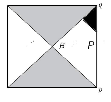
Figure 2: In this diagram, the “exterior” region for a given cut of the future horizon is the region to the right of, and spacelike separated from, the given cut. In the case of a cut along the surface $B$ – the intersection of the past and future horizons of the static patch $P$ – the exterior region is simply $P$. What is exterior to a later cut of the future horizon is a smaller spacetime region, such as the example shaded in black.

The generalized entropy for different horizon cuts can be compared by an elegant formula Wall . A particularly simple and useful case of this formula compares $S_{\mathrm{gen}}(B)$, the generalized entropy of the bifurcate horizon $B$, to $S_{\mathrm{gen}}(\infty)$, the limit of the generalized entropy as the horizon cut goes to future infinity. In this case, the formula reads

$$S_{\mathrm{gen}}(B)=S_{\mathrm{gen}}(\infty)-S_{\mathrm{rel}}(\Phi||\Psi).$$ (51)

Here $S_{\mathrm{rel}}(\Phi||\Psi)$ is the relative entropy between a state $\Phi$ of the bulk fields and the natural de Sitter state $\Psi=\Psi_{\mathrm{dS}}$. The state $\Psi_{\mathrm{dS}}$ (or the Hartle-Hawking state, in the case of a black hole) enters the derivation because its modular Hamiltonian generates time translations, which act as boosts of the horizon, leaving fixed the cut $B$.

To compare these formulas, the first step is to observe that one term in eqn. (48) is the relative entropy in eqn. (51):

$$-S_{\mathrm{rel}}(\Phi||\Psi)=\langle\Phi|\log\Delta_{\Psi|\Phi}|\Phi\rangle=-\langle\Phi|h_{\Psi|\Phi}|\Phi\rangle.$$ (52)

This is indeed Araki’s formula for relative entropy in the general context of von Neumann algebras ArakiThree . In the present discussion, $\Phi$ and $\Psi$ are states of the underlying Type III₁ algebra ${\mathcal{A}}$ of quantum fields in de Sitter space, and Araki’s formula for relative entropy is essentially the only one available. In the more familiar case of an algebra of Type I, with states $\Psi,\Phi$ corresponding respectively to density matrices $\sigma,\rho$, one can show that $-\langle\Phi|\log\Delta_{\Psi|\Phi}|\Phi\rangle={\mathrm{Tr}}\,\rho\log\rho-{\mathrm{Tr}}\,\rho\log\sigma$, where the last formula is a possibly more familiar definition of relative entropy.

So to reconcile our formula (49) with the expected result (51), we need

$$S_{\mathrm{gen}}(\infty)\overset{?}{=}\langle\widehat{\Phi}|h_{\Psi}+\beta x|\widehat{\Phi}\rangle+\int_{-\infty}^{0}{\mathrm{d}}x|f(x)|^{2}(-\log|f(x)|^{2}+\log\beta)+{\mathrm{constant}},$$ (53)

where we include in the formula an additive constant which is not captured by the Type II₁ algebra. Of course, the generalized entropy in the far future is supposed to be

$$S_{\mathrm{gen}}(\infty)=\frac{A(\infty)}{4G_{N}}+S_{\mathrm{out}}(\infty),$$ (54)

where $A(\infty)$ and $S_{\mathrm{out}}(\infty)$ are the horizon area and the entropy outside the horizon in the far future.

Because of the exponential expansion of de Sitter space, typical perturbations cross the horizon and disappear from the static patch in a time of order $\beta$. Hence after a few times $\beta$, the static patch contains an observer in empty de Sitter space. It follows that $S_{\mathrm{out}}(\infty)$ is just the entropy of the observer. In our model, we have attributed to the observer no property except an energy, and therefore the entropy of the observer comes only from fluctuations in energy. We can interpret the term $\int_{-\infty}^{0}{\mathrm{d}}x|f(x)|^{2}(-\log|f(x)|^{2}+\log\beta)$ on the right hand side of eqn. (53) as the entropy in the observer’s energy fluctuations. The time at which this entropy is measured does not matter, since in the model, the observer energy $H_{\mathrm{obs}}=q=-x$ is a conserved quantity. So we identify $\int_{-\infty}^{0}{\mathrm{d}}x|f(x)|^{2}(-\log|f(x)|^{2}+\log\beta)$ as $S_{\mathrm{out}}(\infty)$.

It remains to understand the term $\langle\widehat{\Phi}|h_{\Psi}+\beta x|\widehat{\Phi}\rangle$ in the formula for the entropy. Recall that the conjugation by $e^{-{\mathrm{i}}pH}$ mapped $H_{\mathrm{obs}}=q=-x$ to $-x-H$. It follows that

$$\langle\widehat{\Phi}|h_{\Psi}+\beta x|\widehat{\Phi}\rangle=-\beta\langle H_{\mathrm{obs}}\rangle.$$ (55)

To complete the analysis, one needs the fact that the presence in the center of the static patch of an object of energy $E$, assuming that $E$ is small enough that one can work to linear order in $E$, reduces $A_{\mathrm{hor}}/4G_{N}$, where $A_{\mathrm{hor}}$ is the area of the cosmological horizon, by $\beta E$ Susskind . In four dimensions, for example, the Schwarzschild-de Sitter metric for the case of an object of energy $E$ at the center of the static patch is ${\mathrm{d}}s^{2}=-f(r){\mathrm{d}}t^{2}+\frac{1}{f(r)}{\mathrm{d}}r^{2}+r^{2}{\mathrm{d}}\Omega^{2}$, with

$$f(r)=1-\frac{2GE}{r}-\frac{r^{2}}{r_{\mathrm{dS}}^{2}},$$ (56)

where the de Sitter radius is $r_{\mathrm{dS}}=\beta/2\pi$. The cosmological horizon is at the zero of $f(r)$ that approaches $r_{\mathrm{dS}}$ for $E\to 0$. This is at

$$r_{\mathrm{hor}}=r_{\mathrm{dS}}-GE+{\mathcal{O}}(E^{2}).$$ (57)

The horizon area is $A_{\mathrm{hor}}=4\pi r_{\mathrm{hor}}^{2}$, so

$$\frac{A_{\mathrm{hor}}}{4G_{N}}=\frac{\pi r_{\mathrm{dS}}^{2}}{G_{N}}-2\pi Er_{\mathrm{dS}}+{\mathcal{O}}(E^{2})=\frac{\pi r_{\mathrm{dS}}^{2}}{G_{N}}-\beta E+{\mathcal{O}}(E^{2}).$$ (58)

This shows the claimed shift $-\beta\langle H_{\mathrm{obs}}\rangle$ in the entropy of the horizon due to an object at the center of the static patch.

We can therefore interpret the term $-\beta\langle\widehat{\Phi}|q|\widehat{\Phi}\rangle=-\beta\langle H_{\mathrm{obs}}\rangle$ in eqn. (53) as $A_{{\mathrm{hor}}}/4G_{N}$ or more precisely as the shift in $A_{{\mathrm{hor}}}/4G_{N}$ due to the presence of the observer.

4 Hilbert Spaces

4.1 More On Type II Algebras and Hilbert Spaces

We have described an algebra ${\mathcal{A}}_{P}$ of observables that governs the experiences of an observer in the static patch $P$ of de Sitter space. From the point of view of an observer in $P$, the state of the universe is entirely summarized by a density matrix $\rho\in{\mathcal{A}}_{P}$. This observer has no way to know what there is outside of $P$.

However, if we make a global model of the whole de Sitter space $X$, then we can construct a Hilbert space $\widehat{\mathcal{H}}$ that describes the whole universe. This will give a purification of the density matrix $\rho$. In general, a state $\Psi\in\widehat{\mathcal{H}}$ governs observations both in the static patch $P$ and in the complementary static patch $P^{\prime}$. In this section, we will analyze the Hilbert spaces that result from different assumptions about what is in the patch $P^{\prime}$.

But first we will make a few general remarks about Hilbert space representations and density matrices. As a preliminary, instead of the two static patches $P$ and $P^{\prime}$, let us consider ordinary quantum systems $A$ and $B$ with Hilbert spaces ${\mathcal{H}}_{A}$ and ${\mathcal{H}}_{B}$ that are respectively of dimension $n$ and $m$. The combined system $AB$ has a tensor product Hilbert space ${\mathcal{H}}_{AB}={\mathcal{H}}_{A}\otimes{\mathcal{H}}_{B}$ of dimension $nm$. If and only if $n=m$, any density matrix of either system is the reduced density matrix of a pure state of the combined system. If $n>m$, then any density matrix of system $B$ can be realized by a pure state of the combined system, but this is not true for system $A$. For $n>m$, the maximum entropy of a density matrix of system $A$ that comes from a pure state of the combined system is $\log m$. This is less than the entropy $\log n$ of a maximally mixed state of system $A$ by an “entropy deficit” $\Delta S=\log n-\log m=\log 1/d$, where $d=m/n$. If instead $d>1$, the roles of systems $A$ and $B$ are reversed, and $B$ has an entropy deficit $\log d$.

All of this has a precise analog for an algebra ${\mathcal{A}}$ of Type II₁. The role of $d$ is played by the “continuous dimension” of Murray and von Neumann, which as explained in section 1.3 classifies the representations of ${\mathcal{A}}$ on a Hilbert space. Here $d$ is a positive real number or infinity. When ${\mathcal{A}}$ acts on a Hilbert space, its commutant ${\mathcal{A}}^{\prime}$ is of Type II₁ unless $d=\infty$, in which case it is Type II_∞.

For $d=1$, we can assume that the Hilbert space ${\mathcal{H}}$ is a copy of the algebra ${\mathcal{A}}$ itself. The inner product on ${\mathcal{H}}$ is defined by $({\sf x},{\mathrm{y}})={\mathrm{Tr}}\,{\sf x}^{\dagger}{\mathrm{y}}$, for ${\sf x},{\mathrm{y}}\in{\mathcal{H}}$. The action of ${\mathcal{A}}$ on ${\mathcal{H}}$ is described by ${\sf x}\to{\sf a}{\sf x}$, for ${\sf a}\in{\mathcal{A}}$, ${\sf x}\in{\mathcal{H}}$. The commutant of ${\mathcal{A}}$ is another algebra ${\mathcal{A}}^{\prime}$ that can be described as follows. For any ${\sf a}\in{\mathcal{A}}$, there is an element ${\sf a}^{\prime}\in{\mathcal{A}}^{\prime}$, acting on ${\mathcal{H}}$ by right multiplication, ${\sf x}\to{\sf x}{\sf a}^{\prime}$. (${\mathcal{A}}^{\prime}$ is actually the “opposite algebra” to ${\mathcal{A}}$, with multiplication in the opposite order: $({\sf a}{\sf b})^{\prime}={\sf b}^{\prime}{\sf a}^{\prime}$.) Let $\Psi\in{\mathcal{H}}$ be any pure state. To find the reduced density matrix $\rho$ for the algebra ${\mathcal{A}}$, we compute $(\Psi|{\sf a}|\Psi)=(\Psi,{\sf a}\Psi)={\mathrm{Tr}}\,\Psi^{\dagger}{\sf a}\Psi={\mathrm{Tr}}\,{\sf a}\Psi\Psi^{\dagger}$, where we used the cyclic property of the trace. So $\rho=\Psi\Psi^{\dagger}$. Similarly we can find the density matrix of the same state for the algebra ${\mathcal{A}}^{\prime}$. In this case, $(\Psi|{\sf a}^{\prime}|\Psi)=(\Psi|\Psi{\sf a}^{\prime})={\mathrm{Tr}}\,\Psi^{\dagger}\Psi{\sf a}$ and therefore the density matrix is $\sigma=\Psi^{\dagger}\Psi$.

The formulas $\rho=\Psi\Psi^{\dagger}$, $\sigma=\Psi^{\dagger}\Psi$ show that by taking $\Psi=\rho^{1/2}$ or $\Psi=\sigma^{1/2}$, we can get an arbitrary density matrix $\rho$ or $\sigma$ of algebra ${\mathcal{A}}$ or algebra ${\mathcal{A}}^{\prime}$ as the reduced density matrix of a pure state $\Psi\in{\mathcal{H}}$. The same formulas also imply that ${\mathrm{Tr}}\,\rho^{n}={\mathrm{Tr}}\,\sigma^{n}$, for any $n$, so the von Neumann and Rényi entropies of $\rho$ and $\sigma$ are always equal. All this is as in ordinary quantum mechanics.

To get a Hilbert space representation of ${\mathcal{A}}$ with $d<1$, we can pick a projection operator $\Pi\in{\mathcal{A}}$ of trace $d$. Then, viewing $\Pi$ an an element of ${\mathcal{A}}^{\prime}$, we project onto the subspace ${\mathcal{H}}\Pi\subset{\mathcal{H}}$ consisting of states $\Psi\Pi,$ $\Psi\in{\mathcal{H}}$. The algebra ${\mathcal{A}}$ acts on the left on ${\mathcal{H}}\Pi$ as before. Its commutant consists of operators $\Pi{\sf a}^{\prime}\Pi$, acting on the right by $\Psi\Pi\to\Psi\Pi{\sf a}^{\prime}\Pi$. These operators make an algebra $\widetilde{\mathcal{A}}^{\prime}=\Pi{\mathcal{A}}^{\prime}\Pi$, which is also of Type II₁. The element $\Pi\in{\mathcal{A}}^{\prime}$ is the identity in $\widetilde{\mathcal{A}}^{\prime}$. It is usual in an algebra of Type II₁ to define a normalized trace such that the trace of the identity element is 1. For the algebra $\widetilde{\mathcal{A}}^{\prime}$, the normalized trace is

$$\widetilde{\mathrm{Tr}}\,\Pi{\sf a}^{\prime}\Pi=\frac{1}{{\mathrm{Tr}}\,\Pi}{\mathrm{Tr}}\,\Pi{\sf a}^{\prime}\Pi.$$ (59)

Clearly $\widetilde{\mathrm{Tr}}\,\Pi=1$.

An example of a normalized state in ${\mathcal{H}}\Pi$ is $\Psi=\Pi/({\mathrm{Tr}}\,\Pi)^{1/2}$. Using the property $\Pi^{2}=\Pi$ of a projection operator, one finds that the density matrix of algebra ${\mathcal{A}}$ for this state is $\rho=\Psi\Psi^{\dagger}=\Pi/{\mathrm{Tr}}\,\Pi$. The entropy of this density matrix is

$$S(\rho)=-\log(1/{\mathrm{Tr}}\,\Pi)=-\log(1/d),$$ (60)

as we computed in section 1.3. The normalized density matrix of the same state for the algebra $\widetilde{\mathcal{A}}^{\prime}$ is simply $\sigma=\Pi$, with entropy

$$S(\sigma)=-\widetilde{\mathrm{Tr}}\,\sigma\log\sigma=0.$$ (61)

Thus, as in ordinary quantum mechanics, for $d<1$, there is a pure state of the system, namely $\Pi\in{\mathcal{H}}\Pi$, which has maximum entropy for the second algebra $\widetilde{\mathcal{A}}^{\prime}$, but has an entropy deficit $\log(1/d)$ for ${\mathcal{A}}$.

Now let us consider a general state $\Psi={\sf x}\Pi\in{\mathcal{H}}\Pi$, with ${\sf x}\in{\mathcal{A}}$. For $\Psi$ to be normalized, we need

$$(\Psi,\Psi)={\mathrm{Tr}}\,{\sf x}^{\dagger}{\sf x}\Pi=1.$$ (62)

By similar calculations to those that we have already considered, the density matrix of the state $\Psi$ for the algebra ${\mathcal{A}}$ is $\rho={\sf x}\Pi{\sf x}^{\dagger}$, which satisfies $(\Psi|{\sf a}|\Psi)={\mathrm{Tr}}\,{\sf a}\rho$, for all ${\sf a}\in{\mathcal{A}}$. For $\Pi{\sf a}^{\prime}\Pi\in\widetilde{\mathcal{A}}^{\prime}$, we get $(\Psi|\Pi{\sf a}^{\prime}\Pi|\Psi)={\mathrm{Tr}}\,\Pi{\sf x}^{\dagger}{\sf x}\Pi{\sf a}^{\prime}={\mathrm{Tr}}\,\Pi\,\widetilde{\mathrm{Tr}}\,\Pi{\sf x}^{\dagger}{\sf x}\Pi{\sf a}^{\prime}$. Therefore the density matrix of the same state for $\widetilde{\mathcal{A}}^{\prime}$ is

$$\sigma=({\mathrm{Tr}}\,\Pi)\Pi{\sf x}^{\dagger}{\sf x}\Pi.$$ (63)

These formulas for $\rho$ and $\sigma$ lead to ${\mathrm{Tr}}\,\sigma^{n}=({\mathrm{Tr}}\,\Pi)^{n}{\mathrm{Tr}}\,\rho^{n}$ for any $n$, and therefore $\widetilde{\mathrm{Tr}}\,\sigma^{n}=({\mathrm{Tr}}\,\Pi)^{n-1}\,{\mathrm{Tr}}\,\rho^{n}$. Differentiating with respect to $n$ at $n=1$ to compute $S(\rho)=-{\mathrm{Tr}}\,\rho\log\rho$, $S(\sigma)=-\widetilde{\mathrm{Tr}}\,\sigma\log\sigma$, we get

$$S(\rho)=S(\sigma)-\log(1/{\mathrm{Tr}}\,\Pi)=S(\sigma)-\log(1/d).$$ (64)

We already know that the state $\Psi=\Pi$ has the maximum entropy of any state in ${\mathcal{H}}\Pi$ for the algebra $\widetilde{\mathcal{A}}^{\prime}$, namely $0$, so this formula shows that the same state has the maximum entropy of any state in ${\mathcal{H}}\Pi$ for the algebra ${\mathcal{A}}$, namely $-\log\,1/d$. Thus, similarly to what happened in ordinary quantum mechanics, the maximum entropy state in ${\mathcal{H}}\Pi$ has an entropy deficit $\log 1/d$ for the algebra ${\mathcal{A}}$.

As in ordinary quantum mechanics, exchanging the two algebras ${\mathcal{A}}$ and ${\mathcal{A}}^{\prime}$ has the same effect as replacing $d$ with $1/d$, so we will not consider separately the case $d>1$.

The case that is symmetrical between the two algebras is $d=1$. This suggests that if we place in $P^{\prime}$ an observer identical to the observer in $P$, we might get a Hilbert space representation with $d=1$. We will begin with this case, and show that it does lead to $d=1$. As in the preceding discussion, examples with $d\not=1$ can then be constructed by simply acting with a projection operator in one of the two algebras. The case that there is no observer in $P^{\prime}$ turns out to be troublesome, and we will only be able to offer a conjecture about what happens in this case.

4.2 An Observer in the Second Patch

In section 2.4, we started with a Hilbert space ${\mathcal{H}}$ that describes quantum fields in de Sitter space, with the constraints ignored. The important constraint operator was the operator $H$ that generates future-directed time translations of the static patch $P$, and past-directed time translations of the complementary patch $P^{\prime}$. Then we introduced an observer in $P$ with canonical variables $p,q$, and a Hamiltonian $H_{\mathrm{obs}}=q$, with $q\geq 0$. We now extend this construction to an identical observer in the complementary static patch $P^{\prime}$. This observer has canonical variables $p^{\prime},q^{\prime}$ and Hamiltonian $H^{\prime}_{\mathrm{obs}}=q^{\prime}$, again with $q^{\prime}\geq 0$. The combined Hilbert space, ignoring the Hamiltonian constraint, is therefore now ${\mathcal{H}}\otimes{\mathcal{H}}_{\mathrm{obs}}\otimes{\mathcal{H}}^{\prime}_{\mathrm{obs}}$, where $p,q$ act on the Hilbert space ${\mathcal{H}}_{\mathrm{obs}}$ of the observer in $P$, and $p^{\prime},q^{\prime}$ act on the Hilbert space ${\mathcal{H}}^{\prime}_{\mathrm{obs}}$ of the observer in $P^{\prime}$. For example, we can represent $q$ and $q^{\prime}$ as multiplication operators and set $p=-{\mathrm{i}}\partial/\partial q$, $p^{\prime}=-{\mathrm{i}}\partial/\partial q^{\prime}$, or we can represent $p,p^{\prime}$ by multiplication and $q,q^{\prime}$ by differentiation. We will, to begin with, ignore the conditions $q,q^{\prime}\geq 0$, and impose those conditions at the end by acting on the Hilbert space and the algebras with suitable projection operators.

The constraint operator of the combined system is the total Hamiltonian of the bulk system plus the two observers:

$$\widehat{H}=H+H_{\mathrm{obs}}-H^{\prime}_{\mathrm{obs}}=H+q-q^{\prime}.$$ (65)

The reason for the minus sign multiplying $H^{\prime}_{\mathrm{obs}}$ is that $H$ generates past-directed time translations in the patch $P^{\prime}$; indeed, $H$ is odd under the exchange of the two patches, and the extended constraint operator $\widehat{H}$ has the same property.

We essentially already know from section 2.4 how to describe the algebras of the two patches. The observer in patch $P$, if we ignore the constraint, has access to an algebra ${\mathcal{A}}$ of operators on ${\mathcal{H}}$, and also to the operators $p,q$ on ${\mathcal{H}}_{\mathrm{obs}}$. The combined algebra is ${\mathcal{A}}\otimes B({\mathcal{H}}_{\mathrm{obs}})$, where $B({\mathcal{H}}_{\mathrm{obs}})$ is the algebra of all bounded operators on ${\mathcal{H}}_{\mathrm{obs}}$. Taking the constraint into account at the level of observables just means replacing ${\mathcal{A}}\otimes B({\mathcal{H}}_{\mathrm{obs}})$ with its $\widehat{H}$-invariant part. Relative to section (2.4), the constraint now has an extra contribution $q^{\prime}$, but since this operator commutes with ${\mathcal{A}}\otimes B({\mathcal{H}}_{\mathrm{obs}})$, that makes no difference. Hence the invariant subalgebra of ${\mathcal{A}}\otimes B({\mathcal{H}}_{\mathrm{obs}})$ is the same as it was before; it is generated by $e^{{\mathrm{i}}pH}{\sf a}e^{-{\mathrm{i}}pH}$ for ${\sf a}\in{\mathcal{A}}$, along with $q$. Schematically, the invariant algebra is

$${\mathcal{A}}^{*}_{P}=\{e^{{\mathrm{i}}pH}{\sf a}e^{-{\mathrm{i}}pH},q\},~{}~{}~{}{\sf a}\in{\mathcal{A}}.$$ (66)

The reason for the $*$ in ${\mathcal{A}}_{P}^{*}$ is that we have not yet imposed the conditions $q,q^{\prime}\geq 0$; when those conditions are imposed, we will drop the $*$. The fact that ${\mathcal{A}}_{P}^{*}$ is not affected by the presence of an observer in the patch $P^{\prime}$ is a special case of the fact that an observer in patch $P$ does not know what is in $P^{\prime}$. Similarly, before imposing the constraint, the algebra of the complementary patch $P^{\prime}$ is ${\mathcal{A}}^{\prime}\otimes B({\mathcal{H}}^{\prime}_{\mathrm{obs}})$, where ${\mathcal{A}}^{\prime}$ is the commutant of ${\mathcal{A}}$ acting on ${\mathcal{H}}$. Imposing the constraint means replacing ${\mathcal{A}}^{\prime}\otimes B({\mathcal{H}}^{\prime}_{\mathrm{obs}})$ with its $\widehat{H}$-invariant part, which is generated by $e^{-{\mathrm{i}}p^{\prime}H}{\sf a}^{\prime}e^{{\mathrm{i}}p^{\prime}H}$, ${\sf a}^{\prime}\in{\mathcal{A}}^{\prime}$, along with $q^{\prime}$. Schematically

$${\mathcal{A}}_{P^{\prime}}^{*}=\{e^{-{\mathrm{i}}p^{\prime}H}{\sf a}^{\prime}e^{{\mathrm{i}}p^{\prime}H},q^{\prime}\},~{}~{}~{}{\sf a}^{\prime}\in{\mathcal{A}}^{\prime}.$$ (67)

The algebras ${\mathcal{A}}_{P}^{*}$ and ${\mathcal{A}}_{P^{\prime}}^{*}$ obviously commute.

However, we want to impose the constraint $\widehat{H}$ not just on the operators but on the Hilbert space ${\mathcal{H}}\otimes{\mathcal{H}}_{\mathrm{obs}}\otimes{\mathcal{H}}^{\prime}_{\mathrm{obs}}$. It is straightforward to impose a compact group $G$ of constraints on a Hilbert space: one just restricts to the $G$-invariant subspace of Hilbert space. However, that does not work well for constraints that generate a noncompact group. To understand why, let us consider a simplified case in which the constraint that we wish to impose is just $q^{\prime}$. There is no Hilbert space of states annihilated by $q^{\prime}$, since a state annihilated by $q^{\prime}$ must be proportional to $\delta(q^{\prime})$ and is not normalizable. Our problem is not that different, because $-\widehat{H}=e^{-{\mathrm{i}}p^{\prime}(H+q)}q^{\prime}e^{{\mathrm{i}}p^{\prime}(H+q)}$ is conjugate to $q^{\prime}$. In the case of a constraint $\widehat{H}$ that generates a noncompact group (here the group of time translations of the static patch), rather than requiring a physical state $\Psi$ to satisfy $\widehat{H}\Psi=0$, it is often better to impose an equivalence relation $\Psi\cong\Psi+\widehat{H}\chi$ for any $\chi$. The equivalence classes are called coinvariants, and often one can define a Hilbert space of coinvariants even though there is no Hilbert space of invariants. The space of coinvariants has a natural interpretation in BRST quantization. This is discussed in detail in Appendix B, but for the present case of a single constraint, we will give a brief explanation here. In the case of a single constraint $\widehat{H}$, the BRST complex is defined by introducing a single ghost operator $c$ and a single antighost operator $b$, satisfying $c^{2}=b^{2}=0$, $\{c,b\}=1$. These operators can be realized on a pair of states $|\negthinspace\downarrow\rangle$, $|\negthinspace\uparrow\rangle$, respectively of ghost number 0 and 1, satisfying $|\negthinspace\uparrow\rangle=c|\negthinspace\downarrow\rangle$, $|\negthinspace\downarrow\rangle=b|\negthinspace\uparrow\rangle$. The BRST operator is $Q=c\widehat{H}$. The BRST cohomology is defined as the space of states $\widehat{\Psi}$ with $Q\widehat{\Psi}=0$ modulo the equivalence relation $\widehat{\Psi}\cong\widehat{\Psi}+Q\widehat{\chi}$. The cohomology of ghost number 0 consists of states $\widehat{\Psi}=\Psi|\negthinspace\downarrow\rangle$ annihilated by $Q$. The equivalence relation is vacuous for states of ghost number 0, since there are no states at ghost number $-1$. The condition $Q\widehat{\Psi}=0$ is equivalent to $\widehat{H}\Psi=0$, so the BRST cohomology at ghost number 0 is the space of invariants. At ghost number 1, we have $\widehat{\Psi}=\Psi|\negthinspace\uparrow\rangle$ for some $\Psi$. The constraint $Q\widehat{\Psi}=0$ is vacuous, since there are no states of ghost number 2, and the equivalence relation $\widehat{\Psi}\cong\widehat{\Psi}+Q\widehat{\chi}$ becomes $\Psi\cong\Psi+\widehat{H}\chi$. So the BRST cohomology at ghost number 1 is the space of coinvariants.

The present problem is actually a typical example in which one wants to work with the space of coinvariants. Represent $p^{\prime}$ by multiplication, and $q^{\prime}$ by $q^{\prime}={\mathrm{i}}\partial/\partial p^{\prime}$, and define a map from ${\mathcal{H}}\otimes{\mathcal{H}}_{\mathrm{obs}}\otimes{\mathcal{H}}^{\prime}_{\mathrm{obs}}$ to ${\mathcal{H}}\otimes{\mathcal{H}}_{\mathrm{obs}}$ as follows. View an element $\Psi\in{\mathcal{H}}\otimes{\mathcal{H}}_{\mathrm{obs}}\otimes{\mathcal{H}}^{\prime}_{\mathrm{obs}}$ as a function $\Psi(p^{\prime})$ that is valued in ${\mathcal{H}}\otimes{\mathcal{H}}_{\mathrm{obs}}$. For such a $\Psi$, define $T\Psi\in{\mathcal{H}}\otimes{\mathcal{H}}_{\mathrm{obs}}$ by

$$T\Psi=\int_{-\infty}^{\infty}{\mathrm{d}}p^{\prime}\,e^{{\mathrm{i}}p^{\prime}(H+q)}\Psi(p^{\prime}).$$ (68)

Integration by parts shows that the map $\Psi\to T\Psi$ is invariant under $\Psi\to\Psi+\widehat{H}\chi$, with $\widehat{H}=H+q-{\mathrm{i}}\partial/\partial p^{\prime}$. So $T$ gives a map from the space of coinvariants to ${\mathcal{H}}\otimes{\mathcal{H}}_{\mathrm{obs}}$, and this map is in fact an isomorphism. So the space of coinvariants can be identified with ${\mathcal{H}}\otimes{\mathcal{H}}_{\mathrm{obs}}$, and this is the desired Hilbert space $\widehat{\mathcal{H}}^{*}$ (on which we still have to impose $q,q^{\prime}\geq 0$). Of course, we could have made a similar construction with the role of the two observers exchanged, and then we would have identified $\widehat{\mathcal{H}}^{*}$ with ${\mathcal{H}}\otimes{\mathcal{H}}^{\prime}_{\mathrm{obs}}$.

It remains to determine how the algebras ${\mathcal{A}}_{P}^{*}$ and ${\mathcal{A}}_{P^{\prime}}^{*}$ act on $\widehat{\mathcal{H}}^{*}$. By definition, any operator ${\sf x}$ in either ${\mathcal{A}}_{P}^{*}$ or ${\mathcal{A}}_{P^{\prime}}^{*}$ commutes with $\widehat{H}$ and therefore with the BRST operator $Q$; hence ${\sf x}$ makes sense as an operator on the BRST cohomology at ghost number 1, and therefore, on the space of coinvariants. Since we have identified the space of coinvariants with $\widehat{\mathcal{H}}^{*}={\mathcal{H}}\otimes{\mathcal{H}}_{\mathrm{obs}}$ via the map $T$, there is a unique operator $\widehat{\sf x}$ on $\widehat{\mathcal{H}}^{*}$ such that $\widehat{\sf x}T\Psi=T({\sf x}\Psi)$, and this is the operator by which ${\sf x}$ acts on $\widehat{\mathcal{H}}^{*}$.

When we carry out this procedure for ${\mathcal{A}}_{P}^{*}$, nothing happens. $T$ commutes with the operators $p,q,H$, and ${\sf a}\in{\mathcal{A}}$ from which ${\mathcal{A}}_{P}^{*}$ is constructed. So as an algebra of operators on $\widehat{\mathcal{H}}^{*}$, ${\mathcal{A}}_{P}^{*}=\{e^{{\mathrm{i}}pH}{\sf a}e^{-{\mathrm{i}}pH},q\}$, ${\sf a}\in{\mathcal{A}}$, exactly as in eqn. (67). What happens to ${\mathcal{A}}_{P^{\prime}}^{*}$ is more interesting, since the definition of ${\mathcal{A}}_{P^{\prime}}^{*}$ in eqn. (67) involves operators $q^{\prime},p^{\prime}$ that are eliminated when we identify $\widehat{\mathcal{H}}$ as ${\mathcal{H}}\otimes{\mathcal{H}}_{\mathrm{obs}}$. We find

$$T(e^{-{\mathrm{i}}p^{\prime}H}{\sf a}^{\prime}{e^{{\mathrm{i}}p^{\prime}H}}\Psi)={\sf a}^{\prime}T\Psi$$ (69)

and

$$T(q^{\prime}\Psi)=(H+q)T\Psi.$$ (70)

So as an algebra of operators on $\widehat{\mathcal{H}}$, ${\mathcal{A}}_{P^{\prime}}^{*}$ is generated by ${\sf a}^{\prime}\in{\mathcal{A}}^{\prime}$ along with $H+q$:

$${\mathcal{A}}_{P^{\prime}}^{*}=\{{\sf a}^{\prime},H+q\},~{}~{}~{}~{}~{}{\sf a}^{\prime}\in{\mathcal{A}}^{\prime}.$$ (71)

What we have arrived at in eqns. (67) and (71) is the usual picture of two commuting crossed product algebras acting on ${\mathcal{H}}\otimes L^{2}({\mathbb{R}})$, with $q$ as a multiplication operator on $L^{2}({\mathbb{R}})$. The same construction appears in analyzing a black hole GCP . We will reconsider the black hole in section 5.

As in section 2.4, to put ${\mathcal{A}}_{P}^{*}$ in a standard form, we conjugate by $e^{-{\mathrm{i}}pH}$ and define $x=-q$, leading to

$${\mathcal{A}}_{P}^{*}=\{{\sf a},H+x\},~{}~{}~{}~{}~{}{\sf a}\in{\mathcal{A}}$$ (72)

and

$${\mathcal{A}}_{P^{\prime}}^{*}=\{e^{-{\mathrm{i}}pH}{\sf a}^{\prime}e^{{\mathrm{i}}pH},x\},~{}~{}~{}{\sf a}^{\prime}\in{\mathcal{A}}^{\prime}.$$ (73)

Here

$$p=-{\mathrm{i}}\frac{\partial}{\partial q}={\mathrm{i}}\frac{\partial}{\partial x}.$$ (74)

We still have to impose the conditions $q,q^{\prime}\geq 0$, which now become $H+x\leq 0$ and $x\leq 0$. So we introduce projection operators $\Pi\in{\mathcal{A}}_{P}^{*}$, $\Pi^{\prime}\in{\mathcal{A}}_{P^{\prime}}^{*}$, defined by $\Pi=\Theta(-H-x),$ $\Pi^{\prime}=\Theta(-x)$. Then finally we define the physical Hilbert space in the presence of observers of nonnegative energy by projection

$$\widehat{\mathcal{H}}=\Pi\Pi^{\prime}\widehat{\mathcal{H}}^{*}.$$ (75)

Similarly the physical algebras of the two static patches are

$${\mathcal{A}}_{P}=\Pi{\mathcal{A}}_{P}^{*}\Pi,~{}~{}~{}~{}{\mathcal{A}}_{P^{\prime}}=\Pi^{\prime}{\mathcal{A}}_{P^{\prime}}^{*}\Pi^{\prime}.$$ (76)

The projection operators $\Pi\in{\mathcal{A}}_{\mathcal{P}}^{*}$, $\Pi^{\prime}\in{\mathcal{A}}_{P^{\prime}}^{*}$ become the identity operators in ${\mathcal{A}}_{P}$, ${\mathcal{A}}_{P^{\prime}}$.

We already defined the algebra ${\mathcal{A}}_{P}$ in section 2.4. We showed it to be of Type II₁ and studied its normalized trace. Since the construction is symmetric between the two algebras, ${\mathcal{A}}_{P^{\prime}}$ is also of Type II₁, and we expect that $\widehat{\mathcal{H}}$ has continuous dimension 1 as a representation of ${\mathcal{A}}_{P}$ or of ${\mathcal{A}}_{P^{\prime}}$. This is equivalent to saying that the maximum entropy state of either algebra, with density matrix 1, can be realized by a pure state $\Psi\in\widehat{\mathcal{H}}$. The appropriate state, namely $\Psi_{\mathrm{max}}=\Psi_{\mathrm{dS}}\,\sqrt{\beta_{\mathrm{dS}}}e^{\beta_{\mathrm{dS}}x/2}\Theta(-x)$, was already described in section 2.4 (eqn. (28)). The difference between the present discussion and the previous one is that in section (2.4), ${\mathcal{H}}\otimes L^{2}({\mathbb{R}}_{-})=\Pi({\mathcal{H}}\otimes{\mathcal{H}}_{\mathrm{obs}})$ was introduced arbitrarily as a Hilbert space in which the maximum entropy density matrix of the algebra ${\mathcal{A}}_{P}$ can be purified. Now, instead, we have shown that after a further projection by $\Pi^{\prime}$, $\Pi({\mathcal{H}}\otimes{\mathcal{H}}_{\mathrm{obs}})$ becomes the physical Hilbert space for the case that there are identical observers in the two patches. The further projection by $\Pi^{\prime}$ does not affect the analysis of the density matrix of the state $\Psi_{\mathrm{max}}$ for the algebra ${\mathcal{A}}_{P}$, since $\Pi^{\prime}$ leaves $\Psi_{\mathrm{max}}$ invariant and commutes with ${\mathcal{A}}_{P}$.

As an interesting variant of this, we can consider the case that the complementary patch $P^{\prime}$ contains an observer that is not isomorphic to the observer in $P$. As one simple option, we can assume that the Hamiltonian $H^{\prime}_{\mathrm{obs}}=q^{\prime}$ of the second observer is bounded in the range $a\leq q^{\prime}\leq b$. We do not have to assume that $a\geq 0$, but it is physically natural to do so. Moreover, in that case, the projection operator onto states with $a\leq q^{\prime}\leq b$, namely $\Pi^{\prime}_{[a,b]}=\Theta(b-q^{\prime})\Theta(q^{\prime}-a)=\Theta(b+x)\Theta(-x-a)$, is an element of the algebras ${\mathcal{A}}_{P^{\prime}}$. The computation of ${\mathrm{Tr}}\,\Pi^{\prime}_{[a,b]}$ proceeds precisely as in eqn. (25), except that the integral over $x$ goes over the range $-b\leq x\leq-a$:

$${\mathrm{Tr}}\,\Pi^{\prime}_{[a,b]}=\int_{-b}^{-a}\beta_{\mathrm{dS}}{\mathrm{d}}x\,e^{\beta_{\mathrm{dS}}x}=e^{-\beta_{\mathrm{dS}}a}-e^{-\beta_{\mathrm{dS}}b}.$$ (77)

This illustrates the assertion that a projection operator in a Type II₁ algebra can have any trace between 0 and 1, as discussed in section 1.3.

In the presence of an observer in the patch $P^{\prime}$ with energy bounded in the range $a\leq q^{\prime}\leq b$, the Hilbert space becomes $\widehat{\mathcal{H}}_{[a,b]}=\Pi\,\Pi^{\prime}_{[a,b]}\widehat{\mathcal{H}}^{*}$. The algebra ${\mathcal{A}}_{P}$ is unaffected, but we now have ${\mathcal{A}}_{P^{\prime}}=\Pi^{\prime}_{[a,b]}{\mathcal{A}}_{P^{\prime}}^{*}\Pi^{\prime}_{[a,b]}$. As a representation of ${\mathcal{A}}_{P}$, $\widehat{\mathcal{H}}$ now has continuous dimension $d={\mathrm{Tr}}\,\Pi^{\prime}_{[a,b]}$. As explained in section 4.1, the maximum possible entropy of a pure state in $\widehat{\mathcal{H}}_{[a,b]}$, given that this Hilbert space has continuous dimension $d<1$ for the algebra ${\mathcal{A}}_{P}$, is

$$S_{P,\mathrm{max}}=-\log(1/d)$$ (78)

for the algebra ${\mathcal{A}}_{P}$, and $S_{P^{\prime},\mathrm{max}}=0$ for ${\mathcal{A}}_{P^{\prime}}$. A normalized state that has the maximum possible entropy for each algebra is

$$\Psi_{\mathrm{max},[a,b]}=\frac{1}{\sqrt{{\mathrm{Tr}}\,\Pi^{\prime}_{[a,b]}}}\Pi^{\prime}_{[a,b]}\Psi_{\mathrm{max}}.$$ (79)

The physical meaning of the entropy reduction in the patch $P$ is that as we have removed some qubits from the patch $P^{\prime}$, there is no state in $\widehat{\mathcal{H}}_{[a,b]}$ that describes complete entanglement of all degrees of freedom in $P$ with anything in $P^{\prime}$. On the other hand, the the state $\Psi_{\mathrm{max},[a,b]}$ describes complete entanglement of everything in $P^{\prime}$ with something in $P$.

4.3 No Observer in the Second Patch

If we try to repeat this analysis without assuming the presence of an observer in the static patch, we run into immediate difficulty.

We found in section 4.2 that, assuming there is an observer in the complementary patch $P^{\prime}$, we can incorporate the constraints at the level of Hilbert space states by simply omitting the Hilbert space ${\mathcal{H}}^{\prime}_{\mathrm{obs}}$ of this second observer. Whether there is an observer in the patch $P$ was not important in this argument. In other words, if one assumes that there is an observer in $P^{\prime}$ but none in $P$, then the map $T$ defined in eqn. (68) makes sense as an isomorphism between the space of coinvariants in ${\mathcal{H}}\otimes{\mathcal{H}}^{\prime}_{\mathrm{obs}}$ and ${\mathcal{H}}$. So in this case, the physical Hilbert space on which ${\mathcal{A}}_{P^{\prime}}^{*}$ acts should be just $\widehat{\mathcal{H}}={\mathcal{H}}$.

Since the definition of the map $T$ would make sense with the roles of $P$ and $P^{\prime}$ exchanged, we also seem to learn that if there is an observer in $P$ and none in $P^{\prime}$, the algebra ${\mathcal{A}}_{P}^{*}$ should act on $\widehat{\mathcal{H}}={\mathcal{H}}$. However, this is not the case. Recall from eqn. (71) that, as an algebra of operators on $\widehat{\mathcal{H}}$, ${\mathcal{A}}^{*}_{P^{\prime}}$ is generated by ${\sf a}^{\prime}\in{\mathcal{A}}^{\prime}$ and $H+q$. For the same reason, the action of ${\mathcal{A}}^{*}_{P}$ on ${\mathcal{H}}$ should now be generated by ${\sf a}\in{\mathcal{A}}$ and $H$. As we established earlier, for any representation $\widehat{\mathcal{H}}$ of ${\mathcal{A}}^{*}_{P}$, the commutant algebra ${{\mathcal{A}}^{*}_{P}}^{\prime}$ should be a Type II von Neumann algebra. But the reason that we introduced an observer in the patch $P$ in the first place is that on the Hilbert space ${\mathcal{H}}$ of quantum fields in de Sitter space, there are no operators (except $c$-numbers) that commute with both ${\mathcal{A}}$ and $H$. So ${\mathcal{H}}$ cannot be a representation of ${\mathcal{A}}^{*}_{P}$.

We do not have a definitive resolution of this puzzle, but we will offer a conjecture.

To motivate the conjecture, we start with this question. How much less do we expect the maximum entropy to be if there an observer in $P$ but none in $P^{\prime}$, relative to the case of identical operators in each of the two patches?

To motivate an answer, let us discuss the corrections to the entropy $S_{\mathrm{dS}}$ of de Sitter space. According to Gibbons and Hawking GH , in leading order $S_{\mathrm{dS}}=A/4G_{N}$, where $A$ is the area of the cosmological horizon. They obtained this result by evaluating the path integral for the Euclidean version of de Sitter space, which is simply a sphere. In the approximation of keeping only factors that depend exponentially on $G_{N}$, the result is $e^{-I}$, where $I=-A/4G_{N}$ is the classical action. Gibbons and Hawking interpreted this as $e^{S_{\mathrm{dS}}}$, giving $S_{\mathrm{dS}}=A/4G_{N}$.

A more precise evaluation of the Euclidean path integral would then be expected to give a better approximation to $S_{\mathrm{dS}}$. For our purposes, what is relevant is an extremely simple correction to the original calculation that shifts the entropy by a multiple of $\log G_{N}$. In general, consider a gauge or gravitational theory with a classical action proportional to $1/\lambda$, where $\lambda$ is a coupling parameter. In such a theory, consider a family of classical solutions that depends on $r$ parameters, and assume that the generic element of the family is invariant under an $s$-dimensional group $F$ of gauge symmetries. Then the contribution of this family to the path integral is proportional to $\lambda^{-\frac{1}{2}(r-s)}$ (times $e^{-I}$, with $I$ the action). In the case of gravity, we can use this formula with $\lambda=G_{N}$. As a solution of Einstein’s equations with positive cosmological constant, de Sitter space does not depend on any moduli, so this is a case with $r=0$. On the other hand, the de Sitter group $G_{\mathrm{dS}}={\mathrm{SO}}(D+1)$ is a group of symmetries of this solution, so $s={\mathrm{dim}}\,G_{\mathrm{dS}}$. So a slightly more precise formula for the Euclidean path integral of de Sitter space is $e^{-I}G_{N}^{{\mathrm{dim}}\,G_{\mathrm{dS}}/2}.$ Equating this with $e^{S}$, one finds a logarithmic correction to the de Sitter entropy

$$S_{\mathrm{dS}}=\frac{1}{4G_{N}}-\frac{{\mathrm{dim}}\,G_{\mathrm{dS}}}{2}\log(1/G_{N})+\cdots,$$ (80)

where the omitted terms are of order 1 for $G_{N}\to 0$. This logarithmic correction can be found in eqn. (1.4) of Denef and more explicitly (for some values of $D$) in eqn. (1.12) of that paper.

Now assume that a particular static patch $P$ has been selected by some sort of boundary condition or partial gauge-fixing (see section 4.4) that explicitly breaks $G_{\mathrm{dS}}$ down to the symmetry group of $P$. This group is $G_{P}={\mathbb{R}}\times{\mathrm{SO}}(D-1)$, where ${\mathbb{R}}$ is the group of time translations of $P$, and ${\mathrm{SO}}(D-1)$ is the group of rotations. So the logarithmic correction to the entropy is now $-\frac{1}{2}\left(1+{\mathrm{dim}}\,{\mathrm{SO}}(D-1)\right)\log(1/G_{N})$.

What will happen to the maximum possible entropy if we include an observer in the patch $P$, and nothing in $P^{\prime}$? In this case, we expect no increase in the maximum possible entropy, since in the maximally entropic state of de Sitter space, all modes in $P^{\prime}$ are fully entangled. Adding something to $P$ without adding anything to $P^{\prime}$ does not increase the maximum possible entanglement entropy, which is limited by what there is in $P^{\prime}$. So we expect that if an observer is added in $P$ only, the logarithmic correction to the entropy is unchanged and remains $-\frac{1}{2}(1+{\mathrm{dim}}\,{\mathrm{SO}}(D-1))\log(1/G_{N})$. On the other hand, suppose we add an observer in $P^{\prime}$ who is identical to the observer in $P$. Then the two observers can be maximally entangled. A calculation similar to the Gibbons-Hawking calculation but including the entangled pair of observers is discussed in section 4.4. Intuitively, without getting into details, we should expect that with the observers present, time translations should not be interpreted as a group of unbroken gauge transformations, because time translations act on the degrees of freedom of the observers. However, unless we equip each observer with an orthonormal frame (this option was discussed in section 2.6), rotations are still a group of gauge symmetries. So we expect that the logarithmic correction in the presence of the pair of entangled observers will be just $-\frac{1}{2}{\mathrm{dim}}\,{\mathrm{SO}}(D-1)\log(1/G_{N})$. In other words, omitting an observer from the patch $P^{\prime}$ reduces the maximum entropy by $\frac{1}{2}\log(1/G_{N}),$ up to a remainder that is finite for $G_{N}\to 0$.

With this in mind, let us go back to the question of what is the appropriate Hilbert space $\widehat{\mathcal{H}}$ if there is an observer in the patch $P$ and none in the patch $P^{\prime}$. This Hilbert space is expected to admit an action of the Type II₁ algebra ${\mathcal{A}}_{P}$. It therefore can be characterized by a continuous dimension $d$, and, if $d<1$, the maximum entropy state of ${\mathcal{A}}_{P}$ that can be realized by a pure state in $\widehat{\mathcal{H}}$ has an entropy deficit $\log(1/d)$, as we learned in section 4.1. Since the entropy deficit that we expect as a result of having no observer in $P^{\prime}$ is $\frac{1}{2}\log(1/G_{N}),$ we are led to conjecture that

$$d\sim G_{N}^{1/2}.$$ (81)

If this is the correct answer, then it is not surprising that we do not get a sensible answer when we apply the analysis of section 4.2 to the case of an observer in only one patch, because our analysis only suffices to determine the limit of $d$ for $G_{N}\to 0$, and eqn. (81) says that this limit is the forbidden value $d=0$. If eqn. (81) is correct, some sort of quantum correction is needed in order to get a sensible result. Possibly it is important to take into account fluctuations in the horizon.

4.4 Euclidean Approach

Here we will generalize the Euclidean approach to the de Sitter entropy GH to include a completely entangled pair of observers. The Euclidean approach as traditionally developed computes a function that is called the “entropy” without including an observer; however, it is entirely unclear in what sense the function that is computed actually is an entropy. By including an observer in the Euclidean description, we can describe a calculation that is similar in spirit to the original one GH and that gives a similar answer (with a different coefficient for the logarithmic correction), but does have a clear interpretation in terms of entropy.

With our assumption that an observer is described by operators $p,q$ and Hamiltonian $H=q$, the observer can be described in Lorentz signature by an action $\int{\mathrm{d}}\tau(p\dot{q}-q)$, where $\tau$ is proper time measured along the observer’s worldline. In Euclidean signature, this becomes $\int{\mathrm{d}}\tau(-{\mathrm{i}}p\dot{q}-q)$.

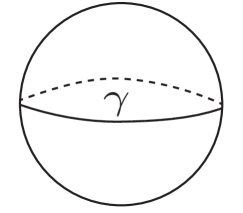
Figure 3: A sphere $S^{D}$ – drawn here for $D=2$ – with a closed geodesic $\gamma$, the Euclidean worldline of the observer.

The Euclidean version of de Sitter space is a sphere $S^{D}$. We assume that the path integral for de Sitter space containing an entangled pair of observers is dominated by a saddle point in which spacetime is $S^{D}$ with a round metric, and the observer worldline is a simple closed geodesic $\gamma\subset S^{D}$ (fig. 3). The circumference of $\gamma$ is $\beta_{\mathrm{dS}}$, the inverse of the de Sitter temperature.

In this situation, if we “cut” $S^{D}$ on a plane of symmetry that is orthogonal to the worldline $\gamma$, and continue to Lorentz signature, then we get a Lorentz signature picture with a pair of observers, one in a static patch $P$ and one in the complementary patch $P^{\prime}$. We expect these two observers to be maximally entangled in a thermofield double state, since in the Euclidean picture they are connected by a finite length worldline.

In Lorentz signature, a particular static patch $P$ can be selected by imposing a boundary condition on the observer’s worldline at past and future infinity. In Euclidean signature, there is no asymptotic region in which a boundary condition can be imposed. Instead, we select a particular closed geodesic $\gamma\subset S^{D}$ by partial gauge-fixing, reducing the symmetry group $G_{\mathrm{dS}}$ of de Sitter space to the symmetry group of a particular geodesic, which is the same as the symmetry group $G_{P}$ of a particular static patch. Taking this into account, the coefficient of the logarithmic correction discussed in section 4.3 is reduced from $-\frac{1}{2}{\mathrm{dim}}\,G_{\mathrm{dS}}$ to $-\frac{1}{2}{\mathrm{dim}}\,G_{P}$.

Apart from this, in the leading approximation for small $G_{N}$, the path integral that we have to do factors as the product of a gravitational path integral, studied originally by Gibbons and Hawking GH and in much more detail recently Denef , and a path integral for the observer.

The path integral of the observer is

$$\int Dp(\tau)\,Dq(\tau)\,\exp\left(\oint_{\gamma}{\mathrm{d}}\tau\left({\mathrm{i}}p\frac{{\mathrm{d}}q}{{\mathrm{d}}\tau}-q\right)\right).$$ (82)

We do first the path integral over $p$. This gives a delta function $\delta({\mathrm{d}}q/{\mathrm{d}}\tau)$. This delta function has two consequences.

First, in doing the path integral over $q$, we can treat $q$ as a constant. The action for the case that $q$ is constant is $\beta_{\mathrm{dS}}q$, so the measure in the integration over the zero-mode of $q$ is $e^{-\beta_{\mathrm{dS}}q}$. Bearing in mind that in analyzing the algebra in section (2.4) we set $x=-q$, this factor is $e^{\beta_{\mathrm{dS}}x}$. We have seen this factor before. The pure state with maximum entropy for the algebra ${\mathcal{A}}_{P}$ of the static patch $P$ was $\Psi_{\mathrm{max}}=\sqrt{\beta_{\mathrm{dS}}}e^{\beta_{\mathrm{dS}}x/2}\Psi_{\mathrm{dS}}$. In a Type I context, such a state would lead to a density matrix proportional to $e^{\beta_{\mathrm{dS}}x}$, although in the usual formalism for Type II algebras, this exponential factor is in the definition of the trace (eqn. (23)) rather than in the density matrix (which is $\rho=1$ for the maximally entropic state).

But the delta function has another and more troublesome consequence. For any periodic function $q(\tau)$, we have $\oint_{\gamma}{\mathrm{d}}\tau\frac{{\mathrm{d}}q}{{\mathrm{d}}\tau}=0$. Therefore the delta function $\delta({\mathrm{d}}q/{\mathrm{d}}\tau)$ that came from the integral over $p$ contains a factor $\delta(0)$. Concretely, this factor comes from the integral over the constant mode of $p$. Formally an infinite factor $\delta(0)$ in the path integral increases the logarithm of the path integral, which is the de Sitter entropy, by an infinite additive constant.

We argued in section 4.3 that adding an entangled pair of observers in the patches $P$ and $P^{\prime}$ increases the maximum possible entropy not by an infinite amount but by an amount of order $\frac{1}{2}\log\,G_{N}$. To get this answer, we would like to replace the factor $\delta(0)$ that came from the path integral over $p$ by a factor $1/G_{N}^{1/2}$. How can we do this?

By taking the Hamiltonian of the observer to be simply $H=q$, we have given a continuous spectrum to the observer and therefore it is natural that incorporating a pair of entangled observers can increase the maximum entanglement entropy by an infinite amount, accounting for the $\delta(0)$. Thus from this point of view, to replace $\delta(0)$ by $1/G_{N}^{1/2}$, we should replace the continuous spectrum of the observer by a discrete spectrum with a level spacing of order $G_{N}^{1/2}$.

A simple way to do this is to replace the Hamitonian $H=q$ of the observer by $H=G_{N}p^{2}+q$, which does indeed lead to a level spacing of order $G_{N}^{1/2}$. If we add this term to the Hamiltonian, then the action likewise has an extra term $G_{N}\oint_{\gamma}{\mathrm{d}}\tau\,p^{2}(\tau)$. For small $G_{N}$, this has no important effect in the preceding calculation except to replace the $\delta(0)$ that came from the integral over the constant mode of $p$ with a factor $1/G_{N}^{1/2}$. Moreover, it seems that a $G_{N}p^{2}$ term in the Hamiltonian of the observer would have played little role elsewhere in this article, since all of our considerations have involved the limit $G_{N}\to 0$.

Although it may be true that adding a term $G_{N}p^{2}$ to the Hamiltonian of the observer makes a better model, there are two things that make us reluctant to propose this as a solution to the problem with the $\delta(0)$. First, it is not clear to us on physical grounds why one should assume that the observer has a level spacing of order $G_{N}^{1/2}$. Second, it is not clear that adding this term to the Hamiltonian of an observer would help in addressing the possibly related puzzle that we ran into in section 4.3, where it was difficult to understand the continuous dimensions of the physical Hilbert space in the case that there is an observer in only one of the two complementary patches. Something more subtle may be needed to deal properly with both the $\delta(0)$ and the continuous dimension.

5 Revisiting the Black Hole

In this section, we will revisit the Type II_∞ algebra of observables exterior to a black hole horizon. One goal is to simplify the arguments that have been presented previously, and formulate them in a way that is not limited to the case of negative cosmological constant. A second goal is to explain that the black hole can be treated quite similarly to the way that we have analyzed de Sitter space in the present article.

For illustration, we will primarily focus on the maximally extended Schwarzschild solution in an asymptotically flat spacetime. However, our arguments apply equally well for AdS Schwarzschild, and we will briefly turn to this setting to discuss the boundary interpretation of the Type II_∞ algebra.

We work in a semiclassical limit in which the Schwarzschild radius $r_{S}$ of the black hole is held fixed, while Newton’s constant $G_{N}\to 0$. This means that the mass of the black hole is very large.

5.1 The Type II_∞ algebra

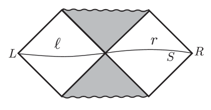
Figure 4: The Penrose diagram of the maximally extended asymptotically flat Schwarzschild spacetime. The left and right exteriors are the unshaded regions labeled $\ell$ and $r$; the left and right regions at spatial infinity are labeled $L$ and $R$. The shaded regions are behind past and future horizons. $S$ is a bulk Cauchy hypersurface, chosen so that it can be decomposed as a union of portions in regions $\ell$ and $r$.

Let $Y$ be the maximally extended Schwarzschild spacetime (fig. 4), and let $\ell$ and $r$ denote the left and right exteriors in $Y$ ($L$ and $R$ will denote left and right spatial infinity). Consider first ordinary quantum field theory in the curved spacetime $Y$. This theory has a Hilbert space $\mathcal{H}_{0}$, and Type III₁ algebras ${\mathcal{A}}_{\ell,0}$ and ${\mathcal{A}}_{r,0}$ of observables in the left and right exterior. The algebras ${\mathcal{A}}_{\ell,0}$ and ${\mathcal{A}}_{r,0}$ are factors (their centers consist only of complex scalars), and they are each other’s commutants.

The spacetime $Y$ has a Killing vector field $V$ that generates time translations. $V$ is future-directed in the right exterior and past-directed in the left exterior. In the quantum theory constructed on $Y$ by expanding around the black hole solution, there is a conserved quantity $\widehat{h}$ associated to $V$. If $S$ is a bulk Cauchy hypersurface, then

$$\widehat{h}=\int_{S}{\mathrm{d}}\Sigma^{\mu}V^{\nu}T_{\mu\nu},$$ (83)

where $T_{\mu\nu}$ is the energy-momentum tensor of the bulk fields (including the energy-momentum pseudo-tensor of the bulk gravitational fluctuations). The operator $\widehat{h}$ has an interpretation in modular theory (or Tomita-Takesaki theory) that is related to the thermal nature of the black hole. Let $\Psi_{HH}$ be the Hartle-Hawking state of the quantum fields on $Y$ HH ; I . Then the modular operator of the state $\Psi_{HH}$ for the algebra ${\mathcal{A}}_{r,0}$ is $\Delta=\exp(-H_{\mathrm{mod}})$ where $H_{\mathrm{mod}}$, known as the modular Hamiltonian, satisfies $H_{\mathrm{mod}}=\beta\widehat{h}$, with $\beta$ the inverse of the Hawking temperature BW ; Sewell .

As in fig 4, one can choose the hypersurface $S$ to pass through the codimension 2 intersection of the left and right horizons. It can then be split as a union $S=S_{\ell}\cup S_{r}$ of portions to the left and right of the horizon. Having done so, it is tempting to define left and right bulk Hamiltonians

$$h_{r}=\int_{S_{r}}{\mathrm{d}}\Sigma^{\mu}V^{\nu}T_{\mu\nu}$$

$$h_{\ell}=-\int_{S_{\ell}}{\mathrm{d}}\Sigma^{\mu}V^{\nu}T_{\mu\nu},$$ (84)

and then

$$\widehat{h}=h_{r}-h_{\ell}.$$ (85)

However, this does not work, because the fluctuations in $h_{r}$ and $h_{\ell}$ are divergent. A modular Hamiltonian of a Type III algebra never has a splitting as in eqn. (85). By contrast, for algebras of Type I or Type II, there is always such a splitting. As we shall see, adding gravity will lead to a splitting of $\widehat{h}$ and to a Type II_∞ algebra.

In the limit $G_{N}\to 0$, local fluctuations of the gravitational field can be treated as just one more field propagating on $Y$. Specifically, for $G_{N}\to 0$, the graviton becomes a massless spin 2 free field, which can be quantized in the usual way. However, adding gravity also introduces additional modes that are not related to local excitations. This is perhaps most obvious in the case of JT gravity in two dimensions. There are no local excitations at all. Nevertheless, JT gravity has a two-dimensional phase space, which was analyzed in detail in JaffHar , for example. The phase space consists by definition of modifications of the geometry along a Cauchy hypersurface $S$ that satisfy natural boundary conditions at infinity, modulo those that can be eliminated by a diffeomorphism of the full spacetime that is trivial at infinity. One such mode is the black hole energy, which in JT gravity is the same whether it is measured in the left or right asymptotic region. In other words, in JT gravity, the left and right Hamiltonians are equal, $H_{L}=H_{R}$. The second mode in JT gravity is more subtle; it involves a shift in the times $t_{L}$ and $t_{R}$ measured at infinity along $S$ on the left and on the right. In other words, a localized perturbation of the geometry along $S$ can have the property that it can be eliminated by a diffeomorphism, but only by a diffeomorphism that acts nontrivially at infinity, shifting the times $t_{L}$ and $t_{R}$ measured along $S$ in the left and right asymptotic regions. Since the Schwarzschild spacetime has a time translation symmetry that shifts $t_{L}$ and $t_{R}$ by equal and opposite amounts, only the sum $\Delta=t_{L}+t_{R}$ is well-defined; thus there is only one mode of this kind.

The time-shift $\Delta$ is not measureable by an observer on either the left or right side of the black hole, so it is not part of the algebra of observables in either exterior region. In JT gravity, the algebras of gauge-invariant observables accessible on the left or right regions outside the horizon are generated, respectively, by $H_{L}$ and $H_{R}$. In particular, these algebras are abelian, and the two algebras coincide, since $H_{L}=H_{R}$. This is quite different from the situation in ordinary quantum field theory, where the left and right algebras ${\mathcal{A}}_{\ell,0}$ and ${\mathcal{A}}_{r,0}$ are factors and their intersection consists only of multiples of the identity.

For Schwarzschild black holes above two dimensions, the time-shift mode is still present, and there are additional modes of a somewhat similar nature that represent a relative rotation between the two asymptotic boundaries. Taking these modes into account, the full Hilbert space in a Schwarzschild spacetime, including perturbative gravitational fluctuations around the Schwarzschild background, is

$$\mathcal{H}\cong\mathcal{H}_{0}\otimes L^{2}({\mathbb{R}}_{t})\otimes L^{2}({\mathrm{SO}}(D-1)),$$ (86)

where $L^{2}({\mathbb{R}}_{t})$ and $L^{2}(SO(D-1))$ are respectively the spaces of square-integrable functions of the time-shift $\Delta$ and of the relative rotation. We give an alternative derivation of this result – making clear the close analogy with the Hilbert space of two observers in de Sitter space – in Section 5.2 below. Of the three factors in ${\mathcal{H}}$, the first, namely ${\mathcal{H}}_{0}$, by itself, admits the action of natural Type III algebras in the left and right exterior regions, just as in ordinary quantum field theory in a Schwarzschild background. Our main goal here is to explain that properly including the second factor $L^{2}({\mathbb{R}}_{t})$ turns the Type III algebras into algebras of Type II_∞. The third factor $L^{2}({\mathrm{SO}}(D-1))$ describes the possibility that the Schwarzschild black hole can acquire spin and become a Kerr black hole. (To be more precise, a slowly rotating black hole can be described by a wavefunction in $L^{2}({\mathrm{SO}}(D-1))$, but if the black hole rotation is not sufficiently slow, one must instead use the nonlinear Einstein equations and the full Kerr solution.) This third factor does not affect the nature of the algebra, and so we will henceforth ignore it for simplicity.

To analyze the algebra of observables in the right exterior region, it is convenient to use the time translation symmetry of the Schwarzschild solution to fix $t_{R}=0$ and therefore $\Delta=t_{L}$. Having made this choice, the coordinate system at spatial infinity in the right exterior is completely fixed. Therefore, it is possible to gravitationally dress bulk operators to the right asymptotic region. To gravitationally dress bulk operators to the left exterior region, we would instead choose $t_{L}=0$, $\Delta=t_{R}$.

Time translations of the left and right boundaries are generated by the ADM Hamiltonians $H_{L}$ and $H_{R}$. We aim to construct an algebra of observables for the right exterior region in the limit $G_{N}\to 0$. In that limit, $H_{L}$ and $H_{R}$ diverge, simply because the black hole mass $M_{0}=r_{S}/2G_{N}$ diverges. It is convenient, therefore, to define subtracted Hamiltonians

$$h_{L}=H_{L}-M_{0},~{}~{}~{}~{}~{}h_{R}=H_{R}-M_{0}$$ (87)

that have limits for $G_{N}\to 0$.

The operator $h_{L}$ generates shifts of $t_{L}$. We can make a unitary transformation to reduce to the case that $h_{L}$ acts only on $t_{L}$, $h_{L}={\mathrm{i}}\frac{\partial}{\partial t_{L}}$, since if instead $h_{L}={\mathrm{i}}\frac{\partial}{\partial t_{L}}+X_{L}$ where $X_{L}$ acts on ${\mathcal{H}}_{0}$, we can remove $X_{L}$ by conjugating with $\exp({\mathrm{i}}t_{L}X_{L})$, and thereby reduce to $h_{L}={\mathrm{i}}\frac{\partial}{\partial t_{L}}$.

The conserved charge $\widehat{h}$ associated to the time translation symmetry of the full spacetime is related to the right and left ADM Hamiltonians by

$$\widehat{h}=H_{R}-H_{L}=h_{R}-h_{L}.$$ (88)

The algebra ${\mathcal{A}}_{r}$ of operators in the right exterior is generated by the algebra ${\mathcal{A}}_{r,0}$ of QFT operators in the right exterior, together with the subtracted right ADM energy $h_{R}=h_{L}+\widehat{h}$. Since $h_{L}$ commutes with everything in ${\mathcal{A}}_{r,0}$, while $\widehat{h}$ generates the modular automorphism group of ${\mathcal{A}}_{r,0}$, this is the crossed product of ${\mathcal{A}}_{r,0}$ by the modular automorphism group of $\Psi_{HH}$, and hence is a Type II_∞ algebra.

The algebra ${\mathcal{A}}_{\ell}$ of operators in the left exterior is generated by the subtracted left ADM energy $h_{L}$, together with $e^{{\mathrm{i}}t_{L}\widehat{h}}{\mathcal{A}}_{\ell,0}e^{-{\mathrm{i}}t_{L}\widehat{h}}$. The conjugation of the left exterior QFT algebra ${\mathcal{A}}_{\ell,0}$ by $e^{{\mathrm{i}}t_{L}\widehat{h}}$ is necessary because we chose a gauge where operators that act solely on $\mathcal{H}_{0}$ are implicitly dressed to the right boundary, and hence are not local to the left exterior. Conjugating by $e^{{\mathrm{i}}t_{L}\widehat{h}}$ shifts this gravitational dressing to the left boundary. Explicitly, one can check that

$$\left[e^{{\mathrm{i}}t_{L}\widehat{h}}{\mathcal{A}}_{\ell,0}e^{-{\mathrm{i}}t_{L}\widehat{h}},h_{L}+\widehat{h}\right]=0~{},$$ (89)

and hence $e^{{\mathrm{i}}t_{L}\widehat{h}}{\mathcal{A}}_{\ell,0}e^{-{\mathrm{i}}t_{L}\widehat{h}}$ commutes with right-boundary time translations. Indeed, the algebra ${\mathcal{A}}_{\ell}$ is the commutant of ${\mathcal{A}}_{r}$, as desired.

5.2 Isometries and Gauge Constraints

We now give an alternative derivation of the Hilbert space and algebra described above that makes the analogy with the de Sitter construction manifest. The isometry group of the asymptotic boundary of the Schwarzschild spacetime $Y$ includes two copies of ${\mathbb{R}}_{t}$ that act separately as time translations of the left and right boundaries. Gauge transformations of the asymptotic boundary are physical degrees of freedom. Hence, before imposing any gauge constraints, we have an “extended Hilbert space”

$$\mathcal{H}^{\mathrm{ext}}\cong\mathcal{H}_{0}\otimes L^{2}({\mathbb{R}}_{t})_{L}\otimes L^{2}({\mathbb{R}}_{t})_{R}~{}.$$

Here, $\mathcal{H}_{0}$ describes the state of the bulk quantum fields, $L^{2}({\mathbb{R}}_{t})_{L}$ describes timeshifts of the left asymptotic boundary, and $L^{2}({\mathbb{R}}_{t})_{R}$ describes the timeshifts of the right asymptotic boundary. Just as in section 5.1, up to conjugation, the left and right subtracted ADM Hamiltonians act solely on $L^{2}({\mathbb{R}}_{t})_{L}$ and $L^{2}({\mathbb{R}}_{t})_{R}$ as $h_{L}={\mathrm{i}}\partial_{t_{L}}$ and $h_{R}={\mathrm{i}}\partial_{t_{R}}$ respectively. The (extended) right exterior algebra consists of

$${\mathcal{A}}_{r}^{\mathrm{ext}}\cong{\mathcal{A}}_{r,0}\otimes B\left(L^{2}({\mathbb{R}}_{t})_{R}\right),$$ (90)

with the left exterior algebra defined analogously.

Note that these are almost the same algebras and Hilbert space that we found for de Sitter space with two observers in section 4.2, before imposing the gauge constraints. The only difference is that the subtracted ADM energies $h_{L}$ and $h_{R}$, unlike the observer energies, do not need to be positive. Instead, $h_{L}$ and $h_{R}$ can take any real values in the semiclassical limit, because of the large constant $r_{S}/2G_{N}$ that has been subtracted when defining them. As in section 2.4, in the absence of a bound on $h_{L}$ and $h_{R}$, the physical algebras will be of Type II_∞ rather than Type II₁.

The final step in deriving those algebras is to impose the isometry group of the full Schwarzschild spacetime as a set of gauge constraints. The relevant isometry group consists of a single copy of ${\mathbb{R}}_{t}$. Because this isometry acts nontrivially at the asymptotic boundary, the correct constraint is not that the bulk isometry generator $\widehat{h}$ annihilates all physical states, but rather that the generator is equal to the corresponding generator in the asymptotic isometry group. In this case, the constraint is exactly (88), namely

$$\widehat{h}=h_{R}-h_{L}$$ (91)

This is the same constraint that we found for observers in de Sitter, except that the energy of the observers has been replaced by minus the subtracted ADM energies.

The problem of how to incorporate such a constraint on the Hilbert space was already discussed in section 4.2. It leads to the elimination of one of the two factors of $L^{2}({\mathbb{R}}_{t})$.

The physical algebra of operators in the right exterior consists of the invariant subalgebra of the extended algebra of operators ${\mathcal{A}}_{r}^{\mathrm{ext}}$ given in eqn. (90). This algebra is generated by $h_{R}$ together with $e^{{\mathrm{i}}t_{R}\widehat{h}}{\mathcal{A}}_{r,0}e^{-{\mathrm{i}}t_{R}\widehat{h}}$. Operators $e^{{\mathrm{i}}t_{R}\widehat{h}}{\mathcal{A}}_{r,0}e^{-{\mathrm{i}}t_{R}\widehat{h}}$ are bulk operators that have been dressed to the right boundary. Similarly the algebra ${\mathcal{A}}_{r}^{\mathrm{ext}}$ is generated by $h_{L}$ together with $e^{-{\mathrm{i}}t_{L}\widehat{h}}{\mathcal{A}}_{l,0}e^{{\mathrm{i}}t_{L}\widehat{h}}$. In the extended Hilbert space description, no operators that act solely on $\mathcal{H}_{0}$ are gauge-invariant; any gauge-invariant operator must be dressed to either the right or the left boundary (or to some combination of the two).

5.3 Boundary Interpretation

If the Schwarzschild spacetime $Y$ is replaced by AdS-Schwarzschild, then the discussion above is completely unchanged. However in this case we know that the bulk gravity theory has a holographic dual. This holographic dual has an associated parameter $N$, such that the $G_{N}\to 0$ limit corresponds to $N\to\infty$. At finite $G_{N}$, the left and right boundary algebras are Type I. We will see that the Type II_∞ algebras describe a particular large $N$ limit of these Type I algebras.

Let us first understand the boundary interpretation of the Hilbert space $\mathcal{H}$ described in (86). For the purposes of illustration, it is helpful to consider the state

$$\ket{\widetilde{\Psi}}=\int{\mathrm{d}}tf(t)\ket{\Psi_{HH}(t)}~{},$$

where $\ket{\Psi_{HH}(t)}=\exp({\mathrm{i}}h_{L}t)\ket{\Psi_{HH}}$ is a timeshifted version of the Hartle-Hawking state. In other words, $\ket{\widetilde{\Psi}}$ is the product of $\ket{\Psi_{HH}}\in\mathcal{H}_{0}$ with some function $f(t)\in L^{2}({\mathbb{R}}_{t})$ that describes a state of the the time-shift mode. The holographic dictionary tells us that the boundary dual of $h_{L}$ is $H_{L}-M_{0}$, where $H_{L}$ is the left boundary Hamiltonian, and the dual of $\ket{\Psi_{HH}}$ is the thermofield double state

$$\ket{\Psi_{\mathrm{TFD}}}=\sum_{i}e^{-\beta E_{i}/2}\ket{i}_{L}\ket{i}_{R}~{},$$ (92)

where the sum is over all energy eigenstates $\ket{i}$. Hence

$$\ket{\widetilde{\Psi}}=\sum_{i}\int{\mathrm{d}}tf(t)e^{{\mathrm{i}}(E_{i}-M_{0})t-\beta E_{i}/2}\ket{i}_{L}\ket{i}_{R}=\sum_{i}\widetilde{f}(E_{i}-M_{0})e^{-\beta E_{i}/2}\ket{i}_{L}\ket{i}_{R}.$$ (93)

In other words, $\ket{\widetilde{\Psi}}$ is dual to a variant of the thermofield state, with finite energy fluctuations that are controlled by the Fourier transform $\widetilde{f}(E_{i}-M_{0})$ of $f(t)$.

Note that to construct the thermofield double state itself we would need to have $f(t)=\delta(t)$. Since $\delta(t)\not\in L^{2}({\mathbb{R}}_{t})$, the large $N$ limit of $\ket{\Psi_{\mathrm{TFD}}}$ does not lie in $\mathcal{H}$. Indeed, in the strict $N\to\infty$ limit, the left and right boundary algebras of any Hilbert space that contains the thermofield double cannot be Type I or II, because the fluctuations in the modular Hamiltonian of the state $\ket{\Psi_{\mathrm{TFD}}}$ diverge at large $N$. If one instead works in a perturbative expansion in $1/N$, then the thermofield double state can be described by a Gaussian wavefunction for the timeshift mode where the energy fluctuations are of order $N$ and hence $\Delta t=O(1/N)$ GCP .

What about states in $\mathcal{H}$ where the QFT degrees of freedom are not in the Hartle-Hawking state? The holographic dictionary tells us that QFT operators in the large $N$ limit are dual to single-trace boundary operators. In fact, the full Hilbert space $\mathcal{H}$ is spanned by states that can be constructed using finite products of single-trace operators from states of the form (93). This is discussed in detail in CPW . The algebras associated to the left and right exteriors are generated by the subtracted Hamiltonians $H_{L/R}-M_{0}$ and single-trace boundary operators.

From a boundary perspective, it is not so surprising that these algebras are Type II, and hence have a finite renormalized trace. At finite $N$, operators whose matrix elements decay sufficiently rapidly at large energy will have a finite Hilbert space trace. For simple operators that are tightly peaked in energy in a finite window around $M_{0}$, this trace should diverge at large $N$ as $\exp(S_{BH})$ times some $N$-independent constant. The Type II algebra trace simply divides out the divergent constant $\exp(S_{BH})$, and keeps the finite piece.

Acknowledgments VC is supported by a grant from the Simons Foundation (816048, VC). GP is supported by the UC Berkeley physics department, the Simons Foundation through the “It from Qubit” program, the Department of Energy via the GeoFlow consortium (QuantISED Award DE-SC0019380) and AFOSR (FA9550-22-1-0098); he also acknowledges support from an IBM Einstein Fellowship at the Institute for Advanced Study. RL acknowledges partial support by MIUR FARE R16X5RB55W QUEST-NET, GNAMPA-INdAM and the MIUR Excellence Department Project awarded to the Department of Mathematics, University of Rome Tor Vergata, CUP E83C18000100006. Research of EW is partly supported by NSF Grant PHY1911298. We thank D. Marolf for remarks on quantization in de Sitter space.

Appendix A Crossed Product and Takesaki Duality

For the convenience of the reader, we recall here a few basic facts on the structure of Connes and Takesaki’s crossed product of a von Neumann algebra by a group action. The crossed product construction is analogous to the semi-direct product in group theory. We refer to T ; vD for a complete exposition.

Crossed product. Let $M$ be a von Neumann algebra on a Hilbert space ${\mathcal{H}}$, $G$ a locally compact group, and $\alpha$ an action of $G$ on $M$; by changing the representation, we may assume that $\alpha$ is implemented by a unitary action $U$ of $G$ on ${\mathcal{H}}$, namely $\alpha={\mathrm{Ad}}\,U$. The crossed product $\widehat{M}=M\rtimes_{\alpha}G$ of $M$ by $\alpha$ is the von Neumann algebra on ${\mathcal{H}}\otimes L^{2}(G)$

$$\widehat{M}=\{x\otimes 1,u(g):x\in M,g\in G\}^{\prime\prime}$$ (94)

(double commutant), where $u(g)=U(g)\otimes\lambda(g)$, with $\lambda$ the left translation unitary representation of $G$ on $L^{2}(G)$. Namely, $\widehat{M}$ is the von Neumann algebra generated by $M\otimes 1$ and $u(g),\,g\in G$. Note that ${\mathrm{Ad}}\,u=\alpha$ on $M$. The construction of $\widehat{M}$ does not depend on the choice of the unitary implementation $U$ of $\alpha$, up to a natural isomorphism.

Let $\beta:G\to{\rm Aut}\,M$ be another action. We shall say that $\alpha$ and $\beta$ are cocycle equivalent if there exists a unitary $\alpha$-cocycle $g\in G\mapsto w(g)\in M$, namely $w(gh)=w(g)\alpha_{g}(w(h))$, $w(\cdot)$ continuous map with $w(g)$ unitary, such that $\beta_{g}(x)=w(g)\alpha_{g}(x)w(g)^{*}$. If $\alpha$ and $\beta$ are cocycle equivalent, there exists a natural isomorphism

$$\{M\rtimes_{\alpha}G,\widehat{\alpha}\}\simeq\{M\rtimes_{\beta}G,\widehat{\beta}\}\,;$$ (95)

this isomorphism is the identity on $M$ and maps $u(g)$ to $w(g)u(g)$.

Dual system. In the following, we assume that $G$ is abelian, denote by $\widehat{G}$ the dual group and by $\langle p,g\rangle$, $p\in\widehat{G},g\in G$, the duality pairing between $\widehat{G}$ and $G$. In the particular, if $G=\mathbb{R}$, we have $\widehat{G}=\mathbb{R}$ and $\langle s,t\rangle=e^{{\mathrm{i}}ts}$.

Let $V$ be the unitary representation of $\widehat{G}$ on $L^{2}(G)$, with $V(p)$ the multiplication by $\langle p,\cdot\rangle$ on $L^{2}$-functions. Then $v=1\otimes V$ implements the action $\widehat{\alpha}$ of $\widehat{G}$ on $\widehat{M}$ given by

$$\widehat{\alpha}_{p}(x)=x,\quad\widehat{\alpha}_{p}(u(g))=\langle p,g\rangle u(g),\quad g\in G,\,p\in\widehat{G},\,x\in M,$$ (96)

(with the identification $x=x\otimes 1$) called the dual action. The $\widehat{\alpha}$-fixed point subalgebra $M^{\widehat{\alpha}}$ is $M$:

$$M=\{x\in\widehat{M}:\widehat{\alpha}_{p}(x)=x,p\in\widehat{G}\}.$$ (97)

Let $\widehat{\widehat{M}}=\widehat{M}\rtimes_{\widehat{\alpha}}\widehat{G}$ be the crossed product of $\widehat{M}$ by $\widehat{\alpha}$. Then $\widehat{M}$ is the $\widehat{\widehat{\alpha}}$-fixed point algebra $\widehat{\widehat{M}}^{\widehat{\widehat{\alpha}}}$ of $\widehat{\widehat{M}}$:

$$\widehat{M}=\{x\in\widehat{\widehat{M}}:\widehat{\widehat{\alpha}}(x)=x\}.$$ (98)

Takesaki duality. Takesaki duality shows the isomorphism of the dynamical systems

$$\{\widehat{\widehat{M}},\widehat{\widehat{\alpha}}\}\simeq\{M\otimes B(L^{2}(G)),\alpha\otimes{\mathrm{Ad}}\,\lambda\}$$ (99)

(${\mathrm{Ad}}\,\lambda$ is the action on $B(L^{2}(G))$ implemented by $\lambda$), namely $M\otimes B(L^{2}(G))$ is isomorphic to $\widehat{\widehat{M}}$ with an isomorphism that interchanges $\alpha\otimes{\mathrm{Ad}}\lambda$ with with $\widehat{\widehat{\alpha}}$. Therefore

$$\big{(}M\otimes B(L^{2}(G))\big{)}^{\alpha\otimes{\rm Ad}\,\lambda}\simeq M\rtimes_{\alpha}G\,.$$ (100)

Dominant and integrable actions. Recall that $M$ is properly infinite if $M$ contains a type I_∞ factor (for example, if $M$ is of type III); equivalently, if $M$ is isomorphic to $M\otimes F$ with $F$ a type I_∞ factor.

By definition, the action $\alpha$ on $M$ is dominant if $M^{\alpha}$ is properly infinite and

$$\{M,\alpha\}\simeq\{M\otimes B(L^{2}(G)),\alpha\otimes{\mathrm{Ad}}\,\lambda\}$$ (101)

(isomorphism of dynamical systems). Then

$$\alpha\ {\rm dominant}\implies M^{\alpha}\ \text{is isomorphic to}\ \widehat{M}\,.$$ (102)

$\alpha$ is dominant iff there exist unitaries $z(p)\in M$, $p\in\widehat{G}$ (Borel family) such that

$$\alpha_{g}(z(p))=\langle p,g\rangle z(p),\quad g\in G,\,p\in\widehat{G}.$$ (103)

The dual action is always dominant. Every action $\alpha$ is cocycle equivalent to a dominant action $\beta$.

The action $\alpha$ is said to be integrable if the linear span of

$$\big{\{}x\in M^{+},\int_{G}\alpha(x)\,{\mathrm{d}}g<\infty\big{\}}$$ (104)

is weakly dense in $M$. Every dominant action is integrable. If $G$ is compact, every action is integrable. Moreover:

$$\alpha\ {\rm integrable}\implies M^{\alpha}\ \text{is isomorphic to a reduced von Neumann subalgebra of $\widehat{M}$}\,,$$ (105)

namely $M^{\alpha}\simeq e\widehat{M}e$ for some projection $e$ of $\widehat{M}$.

Weights, operator-valued weights, dual weights. A normal, faithful, semifinite (n.f.s.) weight $\varphi$ on $M$ is a map $M_{+}\to[0,+\infty]$ (the extended positive real numbers), with $M_{+}$ the cone of positive elements of $M$, such that

$$\varphi(x+y)=\varphi(x)+\varphi(y),\quad\varphi(ax)=a\varphi(x),\quad x,y\in M_{+},\,a\geq 0\,,$$ (106)

with $\sup\varphi(x_{i})=\varphi(\sup x_{i})$ for every bounded, increasing nets $\{x_{i}\}$ in $M_{+}$ (normality), $\varphi(x)=0\implies x=0$, $x\in M_{+}$ (faithfulness), and the linear span $M_{0}$ of the $x\in M_{+}$ such that $\varphi(x)<\infty$ is dense in $M$ (semifiniteness). $\varphi$ can be extended by linearity to all $M_{0}$.

If $N\subset M$ is a von Neumann subalgebra, a n.s.f. operator valued weight $E:M_{+}\to\widetilde{N}_{+}$ is defined similarly as in (106), with $\widetilde{N}$ the extended positive part of $N_{+}$ (see T for the definition of $\widetilde{N}_{+}$), with the property

$$E(n^{*}xn)=n^{*}E(x)n\,,\quad x\in M_{+},\,n\in N\,.$$ (107)

The notion of operator-valued weight, due to Haagerup, generalises the notion of conditional expectation.

Let $\widehat{M}=M\rtimes_{\alpha}G$ be as above. Then

$$T(x)=\int_{\widehat{G}}\widehat{\alpha}_{p}(x)\,{\mathrm{d}}p\,,\quad x\in\widehat{M}_{+}\,,$$ (108)

defines a n.f.s. operator-valued weight $T:\widehat{M}_{+}\to\widetilde{M}_{+}$.

Every n.f.s. weight $\varphi$ of $M$, in particular every normal, faithful state $\varphi$ on $M$, has a canonical lift to a n.f.s. weight $\widehat{\varphi}$ on $\widehat{M}$ given by

$$\widehat{\varphi}=\varphi\cdot T\,;$$ (109)

$\widehat{\varphi}$ is called the dual weight of $\varphi$.

Note that, if $G$ is not discrete, $\widehat{\varphi}(u(t))$ is not defined; however, formally, $\widehat{\varphi}(u(t))=0$, $t\neq 0$. For example, if $G=\mathbb{Z}$, then an element $X$ of $\widehat{M}$ has a Fourier series expansion (in some topology) with Fourier coefficients $x_{n}\in M$, so

$$X=\sum_{n}x_{n}u(n)\ {\rm and}\ \widehat{\varphi}(X)=x_{0}.$$ (110)

If $G=\mathbb{R}$, this is formally true: if $X=\int x(t)u(t)\,{\mathrm{d}}t$, with $x(t)$ a “good” $M$-valued function, then $\widehat{\varphi}(X)=\varphi(x(0))$.

Note also that, if $M={\mathbb{C}}$, then $\widehat{M}$ is $L^{\infty}(\mathbb{R})$ and $\widehat{\varphi}$ is the mean in Fourier transform, namely $\widehat{\varphi}(\lambda(f))=f(0)$, say for a smooth, compactly supported $f$, where $\lambda(f)=\int f(s)\lambda(s){\mathrm{d}}s$.

Crossed product by the modular group. We now specialise the above discussion to the case $G=\mathbb{R}$ and the action $\alpha$ is given by the modular group $\sigma^{\varphi}$ of a faithful normal state $\varphi$ on $M$ (the discussion may be generalized to the case of n.f.s. weights). Thus

$$\widehat{M}=M\rtimes_{\sigma^{\varphi}}\mathbb{R}\,.$$ (111)

By the Connes cocycle Radon-Nikodym theorem, the modular groups associated with different states are cocycle equivalent, therefore $\widehat{M}$ does not depend on the choice of the state $\varphi$, up to a natural isomorphism.

We may define the action $\gamma$ of $\mathbb{R}$ on $\widehat{M}$ by setting

$$\gamma_{s}(x)=\sigma^{\varphi}_{s}(x),\ x\in M,\quad\gamma_{s}(u(t))=u(t),\quad s,t\in\mathbb{R},$$ (112)

indeed $\gamma_{s}={\mathrm{Ad}}\,u(s)$ on $\widehat{M}$. It turns out that $\gamma$ is the modular group $\sigma^{\widehat{\varphi}}$ of the dual weight $\widehat{\varphi}$ of $\varphi$ on $\widehat{M}$. So ${s}^{\widehat{\varphi}}$ is inner. Thus, there exists a trace $\tau$ on $\widehat{M}$ (a n.f.s. weight $\tau$ such that $\tau(z^{*}xz)=\tau(x)$ for all unitaries $z\in\widehat{M}$ and $x\in\widehat{M}_{+}$) given by

$$\tau(\cdot)=\widehat{\varphi}(\rho^{-1}\cdot)\,,$$ (113)

where $u(t)=\rho^{{\mathrm{i}}t}$; $\rho$ is affiliated to $\widehat{M}$, the density matrix of $\widehat{\varphi}$ with respect to $\tau$. Therefore, $\widehat{M}$ is semifinite.

With $\vartheta=\widehat{\sigma}^{\varphi}$ the dual action of $\sigma^{\varphi}$ on $\widehat{M}$, we have $\vartheta_{s}(u(t))=e^{{\mathrm{i}}ts}u(t)$, so $\vartheta_{s}(\rho)=e^{s}\rho$, therefore

$$\tau\cdot\vartheta_{s}=e^{-s}\tau\,,$$ (114)

namely $\vartheta$ is a trace scaling action on $\widehat{M}$.

If $M$ is a type III von Neumann algebra, then $\widehat{M}$ is a type II_∞ von Neumann algebra. If $M$ is a type III₁ factor, then $\widehat{M}$ is a II_∞ factor.

Let $x\in M$ and $f$ a Borel function on $\mathbb{R}$ such that $\int e^{-s}|f(s)|{\mathrm{d}}s<\infty$. Since $\rho^{{\mathrm{i}}t}=U(t)\otimes\lambda(t)$, we have

$$\tau(xf(\log\rho))=\widehat{\varphi}(x\rho^{-1}f(\log\rho))=\varphi(T(x\rho^{-1}f(\log\rho)))$$ (115)

$$~{}~{}~{}~{}~{}~{}~{}~{}~{}~{}~{}~{}~{}~{}~{}~{}~{}~{}~{}=\varphi(x)T(\rho^{-1}f(\log\rho))=\varphi(x)\int e^{-s}f(s){\mathrm{d}}s.$$

In particular, if $f$ is the characteristic function of $[0,\infty)$, the projection $e=f(\log\rho)$ has finite trace: $\tau(e)=\int_{0}^{\infty}e^{-s}{\mathrm{d}}s=1<\infty$.

Appendix B The Hilbert Space of Coinvariants

In this appendix, we will review the construction higuchi ; marolf of a physical Hilbert space for quantum fields coupled to gravity in de Sitter space, in the limit $G\to 0$. Then we will explain how the construction can be naturally placed in the language of BRST cohomology.

B.1 Constraints and Group Averaging

First, we recall the construction of a Hilbert space for a quantum field in de Sitter space $X$, in the absence of gravity CT ; SS ; BD ; Mo ; Al . For illustration, we consider the case of a free scalar field $\phi$ of mass $m$, with action

$$I=-\frac{1}{2}\int{\mathrm{d}}^{D}x\sqrt{\det g}\left(g^{ij}\partial_{i}\phi\partial_{j}\phi+m^{2}\phi^{2}\right).$$ (116)

$\phi$ obeys the massive Klein-Gordon equation

$$\left(-g^{ij}D_{i}D_{j}+m^{2}\right)\phi=0.$$ (117)

By $\Psi_{\mathrm{dS}}$, we mean a state with Gaussian correlations in which the one-point function $\langle\phi(x)\rangle$ vanishes, and the two-point function $\langle\phi(x)\phi(y)\rangle$ is determined by analytic continuation from Euclidean signature. A Hilbert space ${\mathcal{H}}$ that provides an irreducible representation of the canonical commutation relations of the field $\phi$ and contains such a state $\Psi_{\mathrm{dS}}$ can be constructed in an essentially unique way. For this, we observe first that ${\mathcal{H}}$ must contain states obtained by acting on $\Psi_{\mathrm{dS}}$ with any number of $\phi$ fields. So ${\mathcal{H}}$ must contain states

$$\Psi_{f}=\int{\mathrm{d}}x_{1}{\mathrm{d}}x_{2}\cdots{\mathrm{d}}x_{n}f(x_{1},x_{2},\cdots,x_{n})\phi(x_{1})\phi(x_{2})\cdots\phi(x_{n})|\Psi_{\mathrm{dS}}\rangle$$ (118)

where $f(x_{1},x_{2},\cdots,x_{n})$ is any compactly supported function of an $n$-plet of points $x_{1},x_{2},\cdots,$ $x_{n}\in X$. Let ${\mathcal{H}}_{0,n}$ be the space generated by all such states $\Psi_{f}$, where $f$ depends on $n$ points, and let ${\mathcal{H}}_{0}=\oplus_{n=0}^{\infty}{\mathcal{H}}_{0,n}$. The vector $\Psi_{\mathrm{dS}}$ that we started with is an element of ${\mathcal{H}}_{0,0}\subset{\mathcal{H}}_{0}$. Having specified the correlation functions of the field $\phi$ in the state $\Psi_{\mathrm{dS}}$, we immediately know what should be the inner products of states in ${\mathcal{H}}_{0}$. For $\Psi_{f_{1}}\in{\mathcal{H}}_{0,n}$, $\Psi_{f_{2}}\in{\mathcal{H}}_{0,m}$, we define

$$\langle\Psi_{f_{1}},\Psi_{f_{2}}\rangle=\int{\mathrm{d}}x_{1}\cdots{\mathrm{d}}x^{\prime}_{m}\overline{f}_{1}(x_{1},\cdots,x_{n})f_{2}(x^{\prime}_{1},\cdots,x^{\prime}_{m})\langle\Psi_{\mathrm{dS}}|\phi(x_{n})\cdots\phi(x_{1})\phi(x^{\prime}_{1})\cdots\phi(x^{\prime}_{m})|\Psi_{\mathrm{dS}}\rangle.$$ (119)

These integrals always converge, because $f_{1}$ and $f_{2}$ were defined to have compact support. With this inner product, in ${\mathcal{H}}_{0}$ there are many null vectors; for example, if $f=(-g^{ij}D_{i}D_{j}+m^{2})\widetilde{f}$ for some function $\widetilde{f}$ of compact support, then $\Psi_{f}$ is a null vector, because of the Klein-Gordon equation satisfied by $\phi$. Taking the quotient of ${\mathcal{H}}_{0}$ by its null vectors, we get a space ${\mathcal{H}}_{1}$ that has all the properties of a Hilbert space except completeness. Its Hilbert space completion is the Hilbert space ${\mathcal{H}}$ of the massive scalar field in de Sitter space.

Now let us try to couple to gravity, in the limit $G_{N}\to 0$. After turning on gravity, we cannot just consider the fluctuations of matter fields; we have to also construct a Hilbert space of small fluctuations in the metric. This does not change the picture in a qualitative way. What does qualitatively change the picture is that in the presence of gravity, one wishes to impose the symmetry group $G_{\mathrm{dS}}$ as a group of constraints. This is subtle. Naively, for $G_{\mathrm{dS}}$ to be a group of constraints means that states should be $G_{\mathrm{dS}}$-invariant. So one’s first thought is to impose the constraints by restricting from ${\mathcal{H}}$ to its $G_{\mathrm{dS}}$-invariant subspace ${\mathcal{H}}^{G_{\mathrm{dS}}}$. However, there are actually no $G_{\mathrm{dS}}$-invariant vectors in ${\mathcal{H}}$ except multiples of $\Psi_{\mathrm{dS}}$. The definition of ${\mathcal{H}}$ started with a space ${\mathcal{H}}_{0}$ constructed using a function $f$ of compact support on the product of $n$ copies of $X$. The compact support condition trivially means that such states cannot be $G_{\mathrm{dS}}$-invariant for $n>0$. To define ${\mathcal{H}}$, we then took a completion, so that states in ${\mathcal{H}}$ are not necessarily derived from functions of compact support. Nevertheless, states in ${\mathcal{H}}$ are never $G_{\mathrm{dS}}$-invariant. One can define a vector space of $G_{\mathrm{dS}}$-invariant states $\Psi_{f}$, where $f(x_{1},x_{2},\cdots,x_{n})$ is $G_{\mathrm{dS}}$-invariant, but there is no way to define an inner product on the space of such states, since the necessary integral never converges.

Therefore a different procedure is needed. The procedure that works is to consider not invariants in the action of $G_{\mathrm{dS}}$ on the vectors $\Psi_{f}$, but coinvariants. For any $\Psi_{f}\in{\mathcal{H}}_{0}$ and any $g\in G_{\mathrm{dS}}$, we simply declare $\Psi_{f}$ and $g\Psi_{f}$ to be equivalent. The equivalence classes are called coinvariants. We also impose a constraint that $\langle\Psi_{\mathrm{dS}}|\Psi_{f}\rangle=0$ (the purpose of this constraint is to avoid a divergent disconnected contribution in eqn. (120) below). The space of $\Psi_{f}$ subject to the equivalence relation and the constraint defines a new space ${\mathcal{H}}^{\prime}_{0}$, on which $G_{\mathrm{dS}}$ acts trivially by fiat. The formula of eqn. (119) does not define an inner product on ${\mathcal{H}}_{0}^{\prime}$, because in general for $\Psi_{f_{1}},\,\Psi_{f_{2}}\in{\mathcal{H}}_{0}$ and $g\in G_{\mathrm{dS}}$, $\langle\Psi_{f_{1}},\Psi_{f_{2}}\rangle\not=\langle\Psi_{f_{1}},g\Psi_{f_{2}}\rangle$. However, averaging or more precisely integrating over $G_{\mathrm{dS}}$ gives a simple fix. We define

$$\left(\Psi_{f_{1}},\Psi_{f_{2}}\right)=\int_{G_{\mathrm{dS}}}{\mathrm{d}}g\,\langle\Psi_{f_{1}},g\Psi_{f_{2}}\rangle,$$ (120)

where ${\mathrm{d}}g$ is the invariant Haar measure on the $G_{\mathrm{dS}}$ group manifold. It is fairly obvious that if the integral converges, the inner product $(~{},~{})$ is consistent with the equivalence relation (any state of the form $(1-g)\Psi$ is a null vector for this inner product), and therefore the integral defines an inner product on ${\mathcal{H}}_{0}^{\prime}$. The convergence of the integral is subtle; see for example marolf for analysis. Also subtle and not fully understood is the question of whether the inner product defined this way is positive semi-definite. This is known to be the case in some important examples higuchi . We will not address these issues here; our goal is only to explain how group averaging can be interpreted in terms of BRST quantization. Assuming the inner product $(~{},~{})$ exists and is positive semi-definite on the space ${\mathcal{H}}_{0}^{\prime}$, we can proceed as before. We define a space ${\mathcal{H}}_{1}^{\prime}$ as the quotient of ${\mathcal{H}}_{0}^{\prime}$ by null vectors. The Hilbert space completion of ${\mathcal{H}}_{1}^{\prime}$ is then the desired Hilbert space $\widehat{\mathcal{H}}$ taking into account the gravitational constraints.

B.2 The BRST Interpretation

So far, we have just summarized the construction of higuchi ; marolf , which has been called “group averaging” because of the role of integration over $G_{\mathrm{dS}}$ in defining the inner product. In general, group averaging can be naturally understood in a framework of BRST and BV quantization shvedov . Our goal in the rest of this appendix is to explain this point. BRST quantization (rather than the more general BV quantization) is adequate when the constraints generate a Lie algebra, so this approach will suffice.

Let $t_{p}$, $p=1,\cdots,{\mathrm{dim}}\,G_{\mathrm{dS}}$ be the linear operators that generate the action of $G_{\mathrm{dS}}$ on ${\mathcal{H}}_{0}$. They obey

$$[t_{p},t_{q}]=f_{pq}^{r}t_{r},$$ (121)

where $f_{pq}^{r}$ are the structure constants of $G_{\mathrm{dS}}$. Those structure constants obey the Jacobi identity $f_{[pq}^{s}f^{t}_{r]s}=0$, or in more detail

$$f_{pq}^{s}f^{t}_{rs}+f_{qr}^{s}f^{t}_{ps}+f_{rp}^{s}f^{t}_{qs}=0.$$ (122)

Introduce fermion operators $c^{r}$ and $b_{s}$, known respectively as ghosts and antighosts, with anticommutation relations

$$\{c^{r},b_{s}\}=\delta^{r}_{s},~{}\{c^{r},c^{s}\}=\{b_{r},b_{s}\}=0.$$ (123)

Ghost number is defined so that $c^{r}$ has ghost number 1 and $b_{s}$ has ghost number $-1$. The antighost operators have an irreducible representation on a finite-dimensional vector space ${\mathcal{K}}$ that contains a state $|\negthinspace\downarrow\rangle$ of minimum ghost number, with $b_{s}|\negthinspace\downarrow\rangle=0$. Other states in ${\mathcal{K}}$ are obtained by acting on $|\negthinspace\downarrow\rangle$ with a polynomial in the $c$’s. In particular ${\mathcal{K}}$ also contains the state $|\negthinspace\uparrow\rangle=c^{1}c^{2}\cdots c^{{\mathrm{dim}}G_{\mathrm{dS}}}|\negthinspace\downarrow\rangle$ of maximum ghost number, annihilated by the $c$’s. Mathematically, an additive constant in the ghost number is usually fixed so that $|\negthinspace\downarrow\rangle$ has ghost number zero and therefore $|\negthinspace\uparrow\rangle$ has ghost number ${\mathrm{dim}}\,G_{\mathrm{dS}}$. We will use that convention, though physically it is not always the most natural choice.

The group $G_{\mathrm{dS}}$ acts on the combined space ${\mathcal{H}}_{0}\otimes{\mathcal{K}}$ with generators

$$T_{r}=t_{r}-\sum_{s,t}f_{rs}^{t}c^{s}b_{t}.$$ (124)

The BRST operator is defined as

$$Q=\sum_{r}c^{r}t_{r}-\frac{1}{2}\sum_{r,s,t}f_{rs}^{t}c^{r}c^{s}b_{t}.$$ (125)

The factor of $1/2$ is important in verifying the crucial relation

$$Q^{2}=0,$$ (126)

which enables one to define the cohomology of $Q$. The cohomology of $Q$ at ghost number $n$ is defined as the space of states $\Psi$ of ghost number $n$ that satisfy $Q\Psi=0$, modulo those of the form $\Psi=Q\chi$. We denote this cohomology group as $H^{n}(Q,{\mathcal{H}}_{0})$; mathematically, it is called the degree $n$ Lie algebra cohomology of $G_{\mathrm{dS}}$ with values in ${\mathcal{H}}_{0}$. The factor of $1/2$ is also important in verifying the anticommutation relation

$$\{Q,b_{r}\}=T_{r}.$$ (127)

This anticommutation relation ensures that the group generators act trivially on the cohomology of $Q$, since if $Q\Psi=0$, then $T_{r}\Psi=\{Q,b_{r}\}\Psi=Q(b_{r}\Psi)$.

In the BRST approach to quantization, the space of physical states is defined via the cohomology of the BRST operator $Q$ at a specific value of the ghost number. Which is the correct value is somewhat theory-dependent. However, normally there is one specific “allowed” value of the ghost number and physical states are defined in terms of the BRST cohomology at that value of the ghost number. If one did not have this restriction to a particular value of the ghost number, there would be an invariant distinction between physical states based on their ghost number.

In the example of the de Sitter space with weakly coupled gravity, there are two important values of the ghost number, namely the minimum and maximum possible values. A state in ${\mathcal{H}}_{0}\otimes{\mathcal{K}}$ of the minimum possible ghost number is of the general form $\widehat{\Psi}=\Psi\otimes|\negthinspace\downarrow\rangle$, with $\Psi\in{\mathcal{H}}_{0}$. The condition $Q\widehat{\Psi}=0$ reduces to $t_{a}\Psi=0$, in other words $\Psi$ must be $G_{\mathrm{dS}}$-invariant. This is the naive approach to imposing the constraints. As explained earlier, it is unsatisfactory, because except for $\Psi_{\mathrm{dS}}$ itself, there are no $G_{\mathrm{dS}}$-invariant states in ${\mathcal{H}}_{0}$ or in its Hilbert space completion. On the other hand, consider states with the maximum possible ghost number. Such a state has the form $\widehat{\Psi}=\Psi\otimes|\negthinspace\uparrow\rangle$. For such a state, the condition $Q\widehat{\Psi}=0$ is trivial, since the ghost number of $Q\widehat{\Psi}$ exceeds the maximum possible value. However, we need to consider the equivalence relation $\widehat{\Psi}\cong\widehat{\Psi}+Q\chi$. Concretely, a general state of the appropriate ghost number is $\chi=\sum_{a}\chi^{a}b_{a}|\uparrow\rangle$ for some states $\chi^{a}\in{\mathcal{H}}_{0}$. For this choice, the equivalence relation becomes

$$\Psi\cong\Psi+\sum_{a}t_{a}\chi^{a}.$$ (128)

Thus, for states of maximum ghost number, the equivalence relation reduces to an equivalence relation on ${\mathcal{H}}_{0}$, namely $t_{a}\chi\cong 0$ for any state $\chi\in{\mathcal{H}}_{0}$ and for $a=1,\cdots,{\mathrm{dim}}\,G_{\mathrm{dS}}$. This has the same content as the equivalence relation $(1-g)\chi\cong 0$ that we used in discussing group averaging, since from $(1-g)\chi\cong 0$, by differentiating with respect to $g$ at $g=1$ we can deduce that $t_{a}\chi\cong 0$; conversely, from $t_{a}\chi\cong 0$ for all $\chi$, we can deduce $(1-g)\chi\cong 0$ by integration. So in short the top degree cohomology of the BRST operator $Q$ acting on ${\mathcal{H}}_{0}\otimes{\mathcal{K}}$ is the starting point in the construction of the Hilbert space via group averaging.

The rest of the discussion proceeds rather as before, defining an inner product, discarding null vectors, and taking a completion to get a Hilbert space. In the BRST language, the construction of the inner product is naturally described as follows.

First define an indefinite hermitian inner product on ${\mathcal{K}}$ such that $\langle\downarrow|\uparrow\rangle=1$; $c^{r}$, $b_{s}$ are hermitian; and $\langle\Psi,\Psi^{\prime}\rangle=0$ if $\Psi,\Psi^{\prime}$ have ghost number $n,n^{\prime}$ with $n+n^{\prime}\not={\mathrm{dim}}\,G_{\mathrm{dS}}$. These conditions completely determine the inner product; for instance $\langle c^{r}\negthinspace\downarrow|b_{s}\negthinspace\uparrow\rangle=\langle\downarrow|c^{r}b_{s}|\downarrow\rangle=\delta^{r}_{s}$, since $\{c^{r},b_{s}\}=\delta^{r}_{s}$ and $c^{r}|\negthinspace\uparrow\rangle=0$. On ${\mathcal{H}}_{0}^{\prime}\otimes{\mathcal{K}}$, define an inner product $\langle~{},~{}\rangle$ that is the tensor product of the inner product just defined on ${\mathcal{K}}$ and the natural one on ${\mathcal{H}}_{0}^{\prime}$ that was defined in eqn. (119). Then $Q$ is hermitian in this inner product, so $\langle\Psi,\Psi^{\prime}\rangle$, for $\Psi$, $\Psi^{\prime}$ of respective ghost numbers $n$ and ${\mathrm{dim}}\,G_{\mathrm{dS}}-n$, induces a natural sesquilinear map

$$\langle~{},~{}\rangle:H^{n}(Q,{\mathcal{H}}_{0}^{\prime})\times H^{{\mathrm{dim}}\,G_{\mathrm{dS}}-n}(Q,{\mathcal{H}}_{0}^{\prime})\to{\mathbb{C}}.$$ (129)

However, this map is not very useful for our purposes, since physical states lie in $H^{{\mathrm{dim}}\,G_{\mathrm{dS}}}(Q,{\mathcal{H}}_{0}^{\prime})$, which is paired with $H^{0}(Q,{\mathcal{H}}_{0}^{\prime})=0$.

There is a simple way around this. We defined ${\mathcal{H}}_{0}$ in terms of states $\Psi_{f}$ where $f$ has compact support. We can drop the compact support condition and define a “dual” space $\widetilde{\mathcal{H}}_{0}$ generated by states $\Psi_{f}$ with any smooth function $f$, not necessarily of compact support. The inner product $\langle~{},~{}\rangle$ defined in eqn. (119) by integration over a product of copies of $X$ makes sense as a pairing between $\widetilde{\mathcal{H}}_{0}$ and ${\mathcal{H}}_{0}$. (It does not make sense as a pairing between $\widetilde{\mathcal{H}}_{0}$ and itself, which is why it is necessary to base the construction on the cohomology with values in ${\mathcal{H}}_{0}$.) We can define the BRST cohomology $H^{n}(Q,\widetilde{\mathcal{H}}_{0})$ for states valued in $\widetilde{\mathcal{H}}_{0}$, and in particular $H^{0}(Q,\widetilde{\mathcal{H}}_{0})$ is the naive space of unnormalizable states $\Psi_{f}$ with $G_{\mathrm{dS}}$-invariant $f$. As we explained at the beginning, the only trouble with that space is that it is not a Hilbert space in a natural way.

However, the pairing between $\widetilde{\mathcal{H}}_{0}$ and ${\mathcal{H}}_{0}$ that comes from eqn. (119) is useful. Taking the tensor product of this with the inner product on ${\mathcal{K}}$, we get a natural sesquilinear pairing $\langle~{},~{}\rangle:(\widetilde{\mathcal{H}}_{0}\otimes{\mathcal{K}})\times({\mathcal{H}}_{0}\otimes{\mathcal{K}})\to{\mathbb{C}}$ and, since $Q$ is again hermitian, this leads to a much more interesting map

$$\langle~{},~{}\rangle:H^{n}(Q,\widetilde{\mathcal{H}}_{0})\times H^{{\mathrm{dim}}\,G_{\mathrm{dS}}-n}(Q,{\mathcal{H}}_{0}^{\prime})\to{\mathbb{C}}.$$ (130)

Therefore, to define a hermitian inner product on $H^{{\mathrm{dim}}\,G_{\mathrm{dS}}}(Q,{\mathcal{H}}_{0}^{\prime})$, we need a linear map $\eta:H^{{\mathrm{dim}}\,G_{\mathrm{dS}}}(Q,{\mathcal{H}}_{0}^{\prime})\to H^{0}(Q,\widetilde{\mathcal{H}}_{0}^{\prime})$ (sometimes called a rigging map in the literature). Such a map is the composition of $b_{1}b_{2}\cdots b_{n}$ with integration over the action of $G_{\mathrm{dS}}$. The integration operation can be formally denoted $\delta(\vec{T})$, since it projects onto (unnormalizable) states that are annihilated by the $T$’s. Thus $\eta=b_{1}b_{2}\cdots b_{{\mathrm{dim}}\,G_{\mathrm{dS}}}\delta(\vec{T})$. We have $[Q,\eta\}=0$, since $\{Q,b_{r}\}=T_{r}$, $[Q,T_{r}]=0$, and $T_{r}\delta(\vec{T})=0$. So $\eta$ does give a natural map from $H^{{\mathrm{dim}}\,G_{\mathrm{dS}}}(Q,{\mathcal{H}}_{0}^{\prime})$ to $H^{0}(Q,\widetilde{\mathcal{H}}_{0}^{\prime})$. In short, then, from a BRST point of view, the natural hermitian inner product on $H^{{\mathrm{dim}}\,G_{\mathrm{dS}}}(Q,{\mathcal{H}}_{0}^{\prime})$ is

$$(\Psi,\Psi^{\prime})=\langle\Psi|\eta|\Psi^{\prime}\rangle.$$ (131)

Once this inner product is defined, as usual one reduces by null vectors and takes a completion to get the desired Hilbert space $\widehat{\mathcal{H}}$.

One further subtlety is the role of the original de Sitter state $\Psi_{\mathrm{dS}}$. When we summarized the group averaging procedure in Appendix B.1, in addition to imposing an equivalence relation that had the same content as $t_{a}\chi\cong 0$, we also split off $\Psi_{\mathrm{dS}}$ by restricting to states $\Psi_{f}$ that are orthogonal to $\Psi_{\mathrm{dS}}$. This was necessary for convergence of the integral (120). Similarly, in the BRST approach, $\eta$ only makes sense as an operator on ${\mathcal{H}}_{0}^{\prime}$, not on ${\mathcal{H}}_{0}$. However, physically it makes sense that $\Psi_{\mathrm{dS}}$ should be included as a vector in the Hilbert space $\widehat{\mathcal{H}}$ after imposing constraints. We believe that a heuristic explanation is as follows. First of all, the state $\Psi_{\mathrm{dS}}|\negthinspace\uparrow\rangle$ is contained in the BRST cohomology with values in ${\mathcal{H}}_{0}\otimes{\mathcal{K}}$, so the question is how to define its norm. Before imposing the $G_{\mathrm{dS}}$ constraints, the state $\Psi_{\mathrm{dS}}$ is normalizable and one can normalize it to have norm 1. When one imposes the $G_{\mathrm{dS}}$ constraints, one should divide the norm of the $G_{\mathrm{dS}}$-invariant state $\Psi_{\mathrm{dS}}$ by ${\mathrm{vol}}(G_{\mathrm{dS}})$, the (infinite) volume of the de Sitter group. However, when one integrates over the group to define the inner product, in the case of a $G_{\mathrm{dS}}$-invariant state, this just gives back a factor of ${\mathrm{vol}}(G_{\mathrm{dS}})$. In other words, precisely because the Hilbert space inner product is defined by integration over the group, the state $\Psi_{\mathrm{dS}}$ has a nonzero norm after imposing the constraints and survives as a vector in the physical Hilbert space. Obviously, it would be desirable to have an explanation of this point that does not involve canceling the infinite factors of ${\mathrm{vol}}(G_{\mathrm{dS}})$.

B.3 The Observables

In BRST quantization, though the ghosts are important in understanding the physical states, the analysis of the observables is more straightforward. This has been implicitly assumed in the present article, as our main focus has been the algebra of observables in the static patch, and we analyzed this algebra with no mention of the ghosts. The fact that the description of the observables is straightforward can be explained as follows. First of all, in the BRST approach, an observable is defined to be an operator ${\mathcal{O}}$ on the full state space including the ghosts that commutes with $Q$ in the ${\mathbb{Z}}_{2}$-graded sense: $[Q,{\mathcal{O}}\}=0$. This condition ensures that if $Q\Psi=0$, then $Q{\mathcal{O}}\Psi=0$, and also that if $\Psi=Q\chi$, then ${\mathcal{O}}\Psi={\mathcal{O}}Q\chi=(-1)^{{\mathcal{O}}}Q({\mathcal{O}}\chi)$. The two statements together imply that ${\mathcal{O}}$ has a well-defined action on the cohomology of $Q$. Moreover, if ${\mathcal{O}}=[Q,{\mathcal{U}}\}$ for some operator ${\mathcal{U}}$, then ${\mathcal{O}}$ acts trivially on cohomology, since if $Q\Psi=0$ then ${\mathcal{O}}\Psi=[Q,{\mathcal{U}}\}\Psi=Q({\mathcal{U}}\Psi)$. So observables in BRST quantization are defined to be cohomology classes of operators; in other words, an observable is an operator ${\mathcal{O}}$ that satisfies $[Q,{\mathcal{O}}\}=0$, modulo operators of the form $[Q,{\mathcal{U}}\}$.

In general, one shows that at least in the context of perturbation theory (which here means perturbation theory in $G_{N}$) every cohomology class has a representative that can be constructed with no explicit use of $b$. In the present context, this means this means that every operator has a representative constructed only from matter fields and gravity together with the ghost field $c$. Usually, one is primarily interested in operators of ghost number zero. The reason is that as explained in Appendix B.2, normally physical states are defined at just one value of the ghost number (the maximum value, in the case of de Sitter space) and hence an operator of nonzero ghost number has vanishing matrix elements between physical states. An operator of ghost number zero, in its representative that does not contain factors of $b$, automatically also does not depend on $c$; in other words, such an operator is constructed from matter fields and gravity only. If ${\mathcal{O}}$ is an operator that is constructed without any use of either $b$ or $c$, then the condition $[Q,{\mathcal{O}}\}=0$ reduces to $[t_{a},{\mathcal{O}}]=0$. In other words, ${\mathcal{O}}$ must be $G_{\mathrm{dS}}$-invariant.

So while it is subtle to impose the de Sitter constraints on physical states, it is straightforward to impose the constraints on operators: an operator that acts on the constrained system is simply an operator on the unconstrained system that commutes with the constraints. This was assumed in the main body of the paper.

If $\Psi_{1}$, $\Psi_{2}$ are physical states of the constrained system and ${\mathcal{O}}$ is an operator of the constrained system, then

$$\langle\Psi_{1}|g{\mathcal{O}}g^{-1}|\Psi_{2}\rangle=\langle\Psi_{1}|{\mathcal{O}}|\Psi_{2}\rangle,$$ (132)

since physical states were defined to satisfy $g^{-1}\Psi_{1}=\Psi_{1},$ $g^{-1}\Psi_{2}=\Psi_{2}$ (mod $\{Q,\cdots\}$).

We have described this construction for the case of imposing constraints under the full group $G_{\mathrm{dS}}$, but the same ideas apply for imposing constraints under a subgroup such as the symmetry group $G_{P}$ of a static patch $P$. That case is actually much more simple. One has $G_{P}={\mathbb{R}}_{t}\times{\mathrm{SO}}(D-1)$, where ${\mathbb{R}}_{t}$ is the group of time translations of the static patch and ${\mathrm{SO}}(D-1)$ is a group of rotations. The group ${\mathrm{SO}}(D-1)$ is compact, which means that there is no analytical difficulty in defining and understanding the BRST cohomology for ${\mathrm{SO}}(D-1)$ at either the top or bottom value of the ghost number (and these two cohomology groups are actually naturally isomorphic). The group ${\mathbb{R}}_{t}$ of time translations of the static patch is abelian. The group averaging procedure for this abelian group is straightforward and was actually implemented in section 4.

A subtlety in all this accounts for a difficulty that we had in section 4.3. As we have explained, it is possible to identify operators that commute with a set of constraints without first defining a Hilbert space that these operators act on. What one gets this way is an algebra ${\mathcal{B}}_{0}$, but not a von Neumann algebra. To define a von Neumann algebra, one has to construct a Hilbert space $\widehat{\mathcal{H}}$ that ${\mathcal{B}}_{0}$ acts on, and then one can complete ${\mathcal{B}}_{0}$ to a von Neumann algebra ${\mathcal{B}}$ of operators on $\widehat{\mathcal{H}}$. In general, ${\mathcal{B}}$ depends on $\widehat{\mathcal{H}}$. In the main example of the present paper, we start with a Hilbert space ${\mathcal{H}}_{\mathrm{dS}}\otimes L^{2}({\mathbb{R}})\otimes K$, where ${\mathcal{H}}_{\mathrm{dS}}$ is a Hilbert space of fields in de Sitter space, $L^{2}({\mathbb{R}})$ is the Hilbert space of an observer in $P$, and $K$ is the Hilbert space of a possible observer in the complementary patch $P^{\prime}$. An algebra ${\mathcal{A}}$ of the static patch acts on ${\mathcal{H}}$. We consider a constraint $\widehat{H}=H+q-k$, where $H$ generates the time translation symmetry of the patch $P$, $q$ is the Hamiltonian of the observer in $P$, and $k$ acts on $K$. There are two cases of interest: either $K$ is a second copy $L^{2}({\mathbb{R}})^{\prime}$ of $L^{2}({\mathbb{R}})$ and $k=q^{\prime}$ is the Hamiltonian of an observer in $P^{\prime}$, or $K={\mathbb{C}}$, $k=0$. Operators on ${\mathcal{H}}_{\mathrm{dS}}\otimes L^{2}({\mathbb{R}})$ that commute with the constraint are $e^{{\mathrm{i}}pH}{\sf a}e^{-{\mathrm{i}}pH}$ and (bounded functions of) $q$, where $p=-{\mathrm{i}}{\mathrm{d}}/{\mathrm{d}}q$ and ${\sf a}\in{\mathcal{A}}$. These generate an algebra ${\mathcal{B}}_{0}$, which does not depend on whether there is an observer present in $P^{\prime}$. However, the completion of ${\mathcal{B}}_{0}$ to a von Neumann algebra ${\mathcal{B}}$ does depend on the presence of an observer in $P^{\prime}$. In the case $K=L^{2}({\mathbb{R}})^{\prime}$, $k=q^{\prime}$, ${\mathcal{B}}$ is the projected crossed product algebra of Type II₁ that we have studied in this article. In this case, the Hilbert space $\widehat{\mathcal{H}}$ of coinvariants, as a representation of ${\mathcal{B}}$, has a “continuous dimension” in the sense of Murray and von Neumann that can be any positive real number $d$, depending on what we assume for the range of values of $q^{\prime}$. But in case $K={\mathbb{C}}$, $k=0$, in the limit $G_{N}\to 0$, by conjugating by $e^{-{\mathrm{i}}pH}$, we can reduce to the case that the constraint is just $q$ and the Hilbert space $\widehat{\mathcal{H}}$ obtained after imposing the constraint is the original Hilbert space ${\mathcal{H}}_{\mathrm{dS}}$. In that description, ${\mathcal{B}}_{0}$ is generated by ${\mathcal{A}}$ and $H$, and its von Neumann algebra completion is the Type I algebra of all bounded operators on ${\mathcal{H}}$. This is an unreasonable result, since the algebra of operators accessible to an observer in $P$ should not depend in this way on whether there is an observer in $P^{\prime}$. Having no observer in the second patch is similar to taking the limit $d\to 0$ for the continuous dimension of the Hilbert space, but that limit is not possible for an algebra of Type II₁; that is why we seem to get a different algebra in the patch $P$ when there is no observer in $P^{\prime}$. We suggested in section 4.3 that actually it is not possible in this problem to take a strict limit $G_{N}\to 0$, and that in the absence of an observer in $P^{\prime}$, the continuous dimension of $\widehat{\mathcal{H}}$ is $d\sim G_{N}^{1/2}$.

References

- [1] J. D. Bekenstein, “Black Holes and the Second Law,” Lett. Nuovo Cim. 4 (1972) 737-740.
- [2] S. W. Hawking, “Particle Clreation By Black Holes,” Commun. Math. Phys. 43 (1975) 199-220.
- [3] G. W. Gibbons and S. W. Hawking, “Cosmological Event Horizons, Thermodynamics, and Particle Creation,” Phys. Rev. D15 (1977) 2738-2751.
- [4] R. Figari, R. Hoegh-Krohn, and C. R. Nappi, “Interacting Relativistic Boson Fields in the De Sitter Universe With Two Space-Time Dimensions,” Commun. Math. Phys. 44 (1975) 265-278.
- [5] A. Almheiri, T. Hartman, J. Maldacena, E. Shaghoulian, and A. Tajdini, “The Entropy of Hawking Radiation,” Rev. Mod. Phys. 93 (2021) 035002, arXiv:2006.06872.
- [6] R. Bousso, “Positive Vacuum Energy and the Bound,” JHEP 11 (2000) 038, hep-th/0012052.
- [7] R. Bousso, “Bekenstein Bounds in de Sitter and Flat Space,” JHEP 04 (2001) 035, hep-th/0010252.
- [8] T. Banks, “Cosmological Breaking of Supersymmetry? Or Little Lambda Goes Back to the Future, II,” Int. J. Mod. Phys. A16 (2001) 910-921, hep-th/0007146.
- [9] T. Banks and W. Fischler, “-Theory Observables For Cosmological Spacetimes,” arXiv:hep-th/0102077.
- [10] T. Banks, “More Thoughts on the Quantum Theory of Stable de Sitter Space,” arXiv:hep-th/0503066.
- [11] T. Banks, B. Fiol, and A. Morisse, “Towards a Quantum Theory of de Sitter Space,” arXiv:hep-th/0609062.
- [12] T. Banks and W. Fischler, “The Holographic Model Of Cosmology,” arXiv:1806.01749.
- [13] L. Susskind, “De Sitter Holography: Fluctuations, Anomalous Symmetry, and Wormholes,” Universe 7 (2021) 464, arXiv:2106.03964.
- [14] L. Susskind, “Black Holes Hint Towards De Sitter-Matrix Theory,” arXiv:2109.01322.
- [15] K. Maede, T. Koike, M. Narita, A. Ishibashi, “Upper bound for entropy in asymptotically de Sitter space-time,” Phys. Rev. D 57(6) (1998) 3503.
- [16] N. A. Chernikov and E. A. Tagirov, “Quantum theory of scalar field in de Sitter space-time,” Annales de l’Institut Henri Poincaré A IX (1968) 109.
- [17] C. Schomblond and P. Spindel, “Conditions d’unicité pour le propagateur du champ scalaire dans l’univers de de Sitter,” Annales de l’Institut Henri Poincaré A XXV (1976) 67.
- [18] T. S. Bunch and P. Davies, “Quantum Field Theory in de Sitter Space: Renormalization by Point Splitting,” Proc. Roy. Soc. London A360 (1978) 117-34.
- [19] E. Mottola, “Particle Creation in de Sitter Space,” Phys. Rev. D31 (1985) 754.
- [20] B. Allen, “Vacuum States in de Sitter Space,” Phys. Rev. D32 (1985) 3136.
- [21] D. Anninos, F. Denef, Y. T. A. Law, Z. Sun, “Quantum de Sitter Horizon Entropy from Quasicanonical Bulk, Edge, Sphere and Topological String Partition Functions,” arXiv:2009.12464.
- [22] X. Dong, E. Silverstein, and G. Torroba, “De Sitter Holography and Entanglement Entropy,” arXiv:1804.08623.
- [23] H. Lin and L. Susskind, “Infinite Temperature’s Not So Hot,” arXiv:2206.01083.
- [24] S. Leutheusser and H. Liu, “Causal Connectability Between Quantum Systems and the Black Hole Interior in Holographic Duality,” arXiv:2110.05497.
- [25] S. Leutheusser and H. Liu, “Emergent Times in Holographic Duality,” arXiv:2112.12156.
- [26] E. Witten, “Gravity and the Crossed Product,” arXiv:2112.12828.
- [27] R. Sorkin, “On The Entropy of the Vacuum Outside a Horizon,” in B. Bertotti, F. de Felice and A. Pascolini, eds., Tenth International Conference on General Relativity and Gravitation (Padova, July 4-9, 1983), Contributed Papers, vol. II, pp. 734-736 (Roma, Consiglio Nazionale Delle Ricerche, 1983), available at arXiv:1402.3589.
- [28] L. Bombelli, R. K. Koul, Joohan Lee, and R. Sorkin, “Quantum Source of Entropy for Black Holes,” Phys. Rev. D34 (1986) 373-383.
- [29] H. Araki, “Type of von Neumann Algebras Associated to the Free Field,” Prog. Theoret. Phys. 32 (1964) 956.
- [30] I. E. Segal, “A Note On The Concept Of Entropy,” J. Math. Mech. 9 (1960) 623-629.
- [31] R. Longo and E. Witten, “A Note On Continuous Entropy,” arXiv:2202.03357, to appear in Pure and Applied Mathematics Quarterly.
- [32] V. Chandrasekharan, G. Penington, and E. Witten, to appear.
- [33] A. Wall, “A Proof of the Generalized Second Law For Rapidly Changing Fields and Arbitrary Horizon Slices,” Phys. Rev. D85 (2012) 104049, arXiv:1105.3445.
- [34] A. Higuchi, “Quantum linearization instabilities of de Sitter space-time. 1,” Class. Quant. Grav. 8 (1991) 1961 (1991), “Quantum linearization instabilities of de Sitter space-time. 2,” Class. Quant. Grav. 8 (1991) 1983.
- [35] D. Marolf and I. A. Morrison, “Group Averaging for de Sitter Free Fields,” arXiv:0810.5163.
- [36] O. Yu. Shvedov, “On Correspondence of BRST-BV, Dirac, and Refined Algebraic Quantizations of Constrained Systems,” arXiv:hep-th/0111270.
- [37] E. Witten, “Why Does Quantum Field Theory in Curved Spacetime Make Sense? And What Happens to the Algebra of Observables in the Thermodynamic Limit?” arXiv:2112.11614.
- [38] J. B. Hartle and S. W. Hawking, “Path Integral Derivation of Black Hole Radiance,” Phys. Rev. D13 (1976) 2188-2203.
- [39] W. Israel, “Thermo-field Dynamics Of Black Holes,” Phys. Lett. 57 (1976) 107-110.
- [40] W. G. Unruh, “Notes on Black-Hole Evaporation,” Phys. Rev. D14 (1976) 870-892.
- [41] J. Bisognano and E. H. Wichmann, “On The Duality Condition For Quantum Fields,” J. Math. Phys. 17 (1976) 303-21.
- [42] G. L. Sewell, “Quantum Fields On Manifolds: PCT and Gravitationally Induced Thermal States,” Ann. Phys. 141 (1982) 201-24.
- [43] H. J. Borchers, “Uber die Vollständigkeit lorentzinvarianter Felder in einer zeitartigen Röhre,” Nuovo Cimento 19 (1961) 787.
- [44] H. Araki, “A Generalization Of Borchers Theorem,” Helv. Phys. Acta 36 (1963) 132-139.
- [45] A. Strohmaier, “On The Local Structure Of The Klein-Gordon Field On Curved Spacetimes,” Lett. Math. Phys. 54 (2000) 249-61, arXiv:math-ph/0008043.
- [46] M. Takesaki, “Duality for Crossed Products and the Structure of von Neumann Algebras of Type III,” Acta Mathematica 131 (1973) 249-310.
- [47] V. F. R. Jones, “Lectures on Von Neumann Algebras,” available at https://my.vanderbilt.edu/jonesvf/files/2020/10/vonNeumann2015.pdf.
- [48] N. Lashkari, “Modular Zero Modes and the Flow of States of QFT,” JHEP 04 (2021) 189, arXiv:1911.11153.
- [49] E. Witten, “Entanglement Properties of Quantum Field Theory,” Rev. Mod. Phys. 90 (2018), 045003, arXiv:1803.04993.
- [50] H. Araki, “Relative Entropy of States of von Neumann Algebras,” Publ. RIMS, Kyoto Univ. 11 (1976) 809-33.
- [51] D. Jafferis and D. Harlow, “The Factorization Problem in JT Gravity,” JHEP 02 (2020) 177, arXiv:1804.01801.
- [52] M. Takesaki, Theory of Operator Algebras, vol. II, (Springer-Verlag, New York-Heidelberg, 2003).
- [53] A. van Daele, Continuous crossed products and type III von Neumann algebras, LMS Lecture Note Series, 31. Cambridge University Press, Cambridge-New York, 1978.
- [54] M. Henneaux, “Lectures on the Antifield-BRST Formalism for Gauge Theories,” Nucl. Phys. B18A (1990) 47-106.
- [55] D. Marolf, “Group Averaging and Refined Algebraic Quantization: Where Are We Now?”