Moving groups across Galactocentric radius with Gaia DR3

Abstract

The kinematic plane of stars near the Sun has proven an indispensable tool for untangling the complexities of the structure of our Milky Way (MW). With ever improving data, numerous kinematic “moving groups” of stars have been better characterized and new ones continue to be discovered. Here we present an improved method for detecting these groups using MGwave, a new open-source 2D wavelet transformation code that we have developed. Our code implements similar techniques to previous wavelet software; however, we include a more robust significance methodology and also allow for the investigation of underdensities which can eventually provide further information about the MW’s non-axisymmetric features. Applying MGwave to the latest data release from Gaia (DR3), we detect 47 groups of stars with coherent velocities. We reproduce the majority of the previously detected moving groups in addition to identifying three additional significant candidates: one within Arcturus, and two in regions without much substructure at low $V_{R}$. Finally, we have followed these associations of stars beyond the solar neighborhood, from Galactocentric radius of 6.5 to 10 kpc. Most detected groups are extended throughout radius indicating that they are streams of stars possibly due to non-axisymmetric features of the MW.

1 Introduction

Even a relatively small region of the Milky Way (MW) around our Sun contains a wealth of information about the larger properties and non-axisymmetric features of our Galaxy. By studying the motion of nearby stars we can begin to untangle the many complex components of the gravitational potential of the MW including the bar and spiral arms. We have also seen evidence that the stellar disc is out of equilibrium with the discovery of local vertical features like the Radcliffe Wave (Alves et al., 2020) and a more extended vertical kinematic wave (Thulasidharan et al., 2021). Since the Hipparcos mission, scientists have slowly been uncovering more and more detail in the kinematic grouping of stars in the solar neighborhood (“moving groups”; Eggen 1996; Dehnen 1998; Ramos et al. 2018). The intricacies of the azimuthal velocity ($V$; $V_{\phi}$) vs radial velocity ($U$; $V_{R}$) distribution of nearby stars shows that the MW is anything but a smooth galactic disk in dynamical equilibrium (Dehnen, 1998; Antoja et al., 2018). By studying the origin of these substructures with the advent of Gaia (Gaia Collaboration et al., 2016) and, at the same time, utilizing various theoretical approaches (Quillen et al., 2011; Fujii et al., 2019; Monari et al., 2019; D’Onghia & L. Aguerri, 2020; Trick et al., 2021; Craig et al., 2021), we can gain insights on the various components of the MW and understand better galactic structure and evolution.

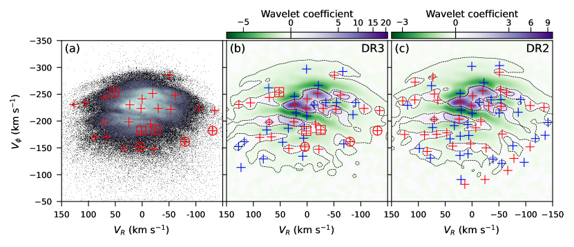
Figure 1: Panel a shows the 2D histogram of all the solar neighborhood stars in the $V_{R}-V_{\phi}$ kinematic plane using Gaia DR3 with a bin size of 0.5 km s^-1. Overplotted are the locations of the wavelet maxima using DR3 data (as in Panel b, see below). Panels b and c show the results of the wavelet transformation for DR3 and DR2, respectively, shown at a scale of 8-16 km s^-1. The purple and green regions depict the relative strength of the positive and negative wavelet coefficients, respectively, normalized by square-root. Contours are shown at the -0.1% (dashed) and the 5% levels. Red markers represent significant overdensities and blue markers represent significant under-densities. Note that only extrema with confidence level $\geq 2$ and $P_{\mathrm{MC}}>0.8$ are shown. The DR3 overdensities are also shown overlaid onto panel (a). In panels (a) and (b) the three new group candidates (DR3G-25, 26, and 31) are circled and those groups previously detected but missing from prior studies using Gaia are enclosed within squares (Kushniruk17-J4-19, HR1614, and Zhao09-9; marked with asterisks in Table 1).

One of the least well-constrained features of the MW is its bar. This non-axisymmetric feature can have a significant gravitational potential and can affect the distribution of stars through resonances. Depending on the length and pattern speed of the bar, it could provide different explanations for many of the moving groups that we see in the solar neighborhood (SN). For example, previous models of the MW included a short bar with a pattern speed of $\sim$55 km s^-1 kpc^-1where the outer Lindblad resonance (OLR) coincided with the SN (Dehnen, 2000; Debattista et al., 2002; Monari et al., 2017). The OLR creates a bimodality in the kinematic plane of stars around the sun providing one possible explanation for the Hercules group. However, recent observations before Gaia DR3 already suggest that the bar is actually long and rotating more slowly ($\sim$40 km s^-1 kpc^-1; Clarke et al. 2019; Sanders et al. 2019). Theoretical models and simulations have shown that Hercules could be formed by stars at the corotation resonance of a long bar (Pérez-Villegas et al., 2017; D’Onghia & L. Aguerri, 2020; Asano et al., 2020). Furthermore, several of the significant moving groups in the solar neighborhood are explained by being in resonance with the long bar (the Outer Lindblad resonance (2:1), the 4:1 or the Outer Ultra-Harmonic resonance, and the 6:1 correspond to the Hat, Sirius, and the Horn, respectively; Monari et al. 2019). The MW’s spiral arms have also been shown to have a significant effect on the kinematics of the SN (e.g. Antoja et al., 2009; Hunt et al., 2018; Michtchenko et al., 2018; Barros et al., 2020). While looking at the resonances in the solar neighborhood alone are not sufficient to break the degeneracy to discriminate between the long and short bar scenarios (Trick et al., 2021; Trick, 2022), Gaia DR3 provided the data to observe the bar in the azimuthal velocity field of the galaxy and indicate that the pattern speed is between 38-42 km/s/kpc (Gaia Collaboration et al., 2022b).

Gaia constitutes the largest and most precise database of positions and velocities of stars in the MW to date, which makes it perfect for this exploration (Gaia Collaboration et al., 2016). Its latest release (Data Release 3; DR3; Gaia Collaboration et al. 2022a) provides improved astrometry and errors for 1.4 billion stars based on 34 months of data. For this study, we include approximately 34 million stars centered on the Sun for which Gaia provides positions, proper motions, parallaxes, and radial velocities.

While much of the structure in the $V_{R}-V_{\phi}$ kinematic diagram is clearly visible as overdensities (e.g. Figure 1a), more sophisticated methods are required to quantify the wealth of information. One such technique is the wavelet transformation. Much like a Fourier transformation, the wavelet transform (WT) decomposes data into different components based on a given scale (see Starck et al., 1998, and references therein). When applied to 2D images, the WT can isolate visual structures of different sizes. This technique has been used on a variety of astrophysical data where it allows for the detection of subtle variations from uniformity, e.g. cosmological large-scale structure (Slezak et al., 1993; Einasto et al., 2011), galaxy cluster distributions (Girardi et al., 1997; Da Rocha & Mendes de Oliveira, 2005; Da Rocha et al., 2008), and the cosmic microwave background (Sanz et al., 1999; Rogers et al., 2016; Hergt et al., 2017).

Recent work has also utilized the WT to explore the kinematic space of the MW (Antoja et al., 2008; Zhao et al., 2009; Zhao et al., 2014, 2015; Kushniruk et al., 2017; Ramos et al., 2018; Yang et al., 2021; Bernet et al., 2022). Ramos et al. (2018) (hereafter R18) used Gaia DR2 and the WT to detect moving groups in the $V_{R}-V_{\phi}$ plane and found many arch features covering the majority of previously known moving groups. In addition to detecting 28 new overdensities, they traced $V_{\phi}$ of the groups over radius and azimuth to compare with the detected ridges in $V_{\phi}-R$ space (Antoja et al., 2018). The outcome showed that there are kinematic features indicative of both phase mixing processes as well as resonant trapping due to the MW’s non-axisymmetric structures.

Similarly, Bernet et al. (2022) explored a larger region of the MW disk using Gaia eDR3 and the WT combined with a breadth-first search to group detected overdensities together in $(R,\phi,Z,V_{R},V_{\phi})$ space. The WT they use is one-dimensional and was specifically designed to detect and group overdensities into the arches found in R18. They again explore the variation in $V_{\phi}$ vs $R$ for each detected group in addition to looking at the distribution of $V_{\phi}$ along $\phi$ and $z$. By comparing with both slow- and fast-bar models, they find several resonances that overlap with the detected groups/arches, however Gaia eDR3 was not extended enough to determine the bar’s length and pattern speed in order to remove the degeneracy.

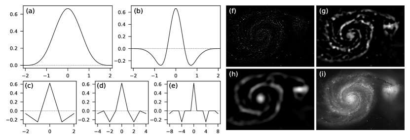
Figure 2: Panels a and b show the continuous B3-spline scaling function, $\phi(x)$, and the corresponding wavelet function, $\psi(x)$, respectively. Panels c$-$e show the discrete wavelet function (generated from the filters $h$ and $g$) for scales $j=0$, $j=1$, and $j=2$. Panels f$-$h show the resulting wavelet transform of the image of M51 shown in panel i.  The original image is 720 pixels wide by 1037 pixels high and the scales shown in panels f, g, and h are $j=2$, $j=4$, and $j=5$ resulting in the detection of features with sizes of 4-8 pixels, 16-32 pixels, and 32-64 pixels respectively.

For this work, we have developed an open-source WT code for use in Python, MGwave. The code is based on the á trous algorithm (Starck & Murtagh, 1994; Starck et al., 1998) and is able to perform the wavelet transformation on any 2D image and output the resultant wavelet coefficients, locations of the extrema, as well as a significance, or confidence level for each extremum (when compared to values resulting from Poisson noise). We build on previous works by using our MGwave code to analyze the SN as seen by Gaia DR3. By performing the full 2D WT, we not only detect new kinematic moving groups, but we are also able to track their extension in the kinematic plane and their location through Galactocentric radius. By identifying moving groups of stars that are extended across the Galactic disk, we can distinguish the large-scale substructures with a dynamical origin (e.g. those stars that might be in resonance with the bar or spiral arms) from local, transient features.

This paper is structured as follows: Section 2 outlines our data sample and WT methods, Section 3 shows the main results, Section 4 discusses the implications of our results within the context of previous works, and conclusions are summarized in Section 5.

2 Methods

2.1 Gaia Data Sample

We selected from the approximately 34 million stars that have positions, proper motions, parallaxes, and radial velocities in Gaia DR3. In order to avoid the known biases caused by inverting the parallax to find distances, we use the geometric distances, along with their errors, computed by Bailer-Jones et al. (2021) (Bailer-Jones et al., 2020). We transformed the six-dimensional Gaia observables to Galactocentric cylindrical coordinates with the sun located at $\phi_{\odot}=0^{\circ}$, $Z_{\odot}=5.5$ pc, and $R_{\odot}=8.15$ kpc. We take the peculiar motion of the sun with respect to the local standard of rest (LSR) in cartesian coordinates as $(U,V,W)=(10.6,10.7,7.6)$ km s^-1 and the circular velocity of the sun as $V_{c}=236$ km $s^{-1}$ (Reid et al., 2019). $V_{R}$ is directed out away from the Galactic center and $V_{\phi}$ is directed against the direction of rotation of the disk (i.e. $\phi$ decreases in the direction of rotation, towards the major axis of the MW bar, and increases counter to the rotation, towards the minor axis of the MW bar).

We used Monte Carlo simulations to transform the Gaia errors from right ascention, declination, proper motions, and radial velocities (source properties) into the Galactocentric cylindrical coordinates defined above (final properties). Using the pyia code (Price-Whelan, 2018), we sampled the source Gaia data 256 times for each star, assuming a gaussian distribution for each property. By then transforming the sampled properties into Galactocentric coordinates, we could measure the spread in their values (the standard deviation) to determine the errors in the final properties ($R$, $\phi$, $Z$, $V_{R}$, $V_{\phi}$, $V_{Z}$). This method does account for correlations between right ascention, declination, and proper motion, but does not include correlations for radial velocity or the Bailer-Jones distances.

There are 33,653,049 stars with radial velocities and Bailer-Jones distances in Gaia DR3. This is increased by more than a factor of four over eDR3. We define the “solar neighborhood” region as $|z|<0.5$ kpc, $-1.5^{\circ}<\phi<1.5^{\circ}$, and $8.05<R<8.25$ kpc which contains 997,918 stars. We have also explored additional volumes throughout the Galactic disk by looking at 70 overlapping radial bins of width 0.2 kpc in the range $R=$ (6.4, 10.1) kpc while maintaining the constraints on $z$ and $\phi$, specifically (6.4, 6.6) kpc, (6.45, 6.65) kpc, (6.5, 6.7) kpc, etc. However, we do see a decrease in the number of stars per bin as we reach the limits of this range.

In order to compare with previous works, we have also performed the same analysis with Gaia’s Data Release 2 (DR2). We have followed the same procedure as above however we have used the definition of Galactocentric cylindrical coordinates as defined in R18 ($Z_{\odot}=14$ pc, $R_{\odot}=8.34$ kpc, $(U,V,W)=(11.1,12.24,7.25)$ km s^-1, and $V_{c}=240$ km $s^{-1}$ from Schönrich et al. 2010 and Reid et al. 2014). We have also required “good” parallax values, i.e. $\omega/\sigma_{\omega}>5$ and distances were calculated by inverting the parallax. This provided us with an identical data set to that of R18. A comparison of our results between DR2 and DR3 is shown in Figure 1.

Figure 3: Wavelet coefficient values across the kinematic plane for the solar neighborhood at various wavelet scales using Gaia DR3. Panel (a) corresponds to a scale of $j=2$ increasing to a scale of $j=5$ in Panel (d). Given our bin size of 0.5 km s^-1, these correspond to physical sizes of 2 km s^-1 up to 32 km s^-1 (see labels in figure). Contours are shown at the 5% and -0.1% (dashed) level (except for Panel (a)).

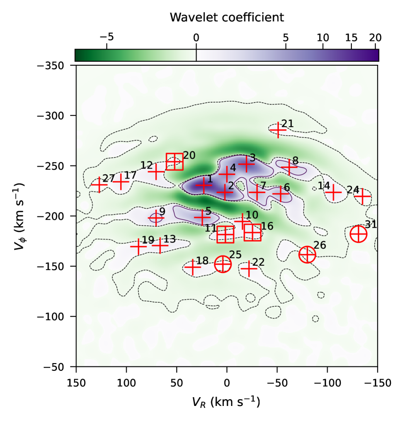
Figure 4: As Figure 1b with only maxima shown and numbered by ID as listed in Table 1. Again, only maxima with confidence level $\geq 2$ and $P_{\mathrm{MC}}>0.8$ are plotted, with circles enclosing the three new group candidates and squares around the three groups not previously seen within Gaia data.

2.2 Wavelet Transform Method

Our open-source WT code, MGwave, is based on the á trous algorithm (Starck & Murtagh, 1994; Starck et al., 1998). We have also implemented quantitative analysis to determine the significance of detected structures with respect to Poisson noise (Slezak et al., 1993). Finally, Monte Carlo simulations are used to propagate data errors through to the wavelet results.

Our implementation of the á trous algorithm utilizes the Starlet transformation with a B3-spline scaling function (Starck & Murtagh, 2006),

$$\phi(x)=B_{3}(x)=\\ \frac{1}{12}\left(|x-2|^{3}-4|x-1|^{3}+6|x|^{3}-4|x+1|^{3}+|x+2|^{3}\right).$$ (1)

Figures 2a and b shows the continuous scaling function and corresponding wavelet function. Since we are working with pixellated images, we need to discretize these functions. Defined in terms of the $h$ and $g$ filter set (Starck et al., 1998), the scaling function corresponds to $h=[\frac{1}{16},\frac{1}{4},\frac{3}{8},\frac{1}{4},\frac{1}{16}]$ and the wavelet function is derived from $g=\delta-h=[-\frac{1}{16},-\frac{1}{4},\frac{5}{8},-\frac{1}{4},-\frac{1}{16}]$ (where $\delta$ is the discretized delta function, i.e. $\delta=[0,0,1,0,0]$). These discrete wavelet functions are shown in Figure 2c$-$e for three different scales ($j=0$, $j=1$, and $j=2$). By applying this separable convolution mask to our image in each dimension sequentially, we obtain the wavelet transformed image (consisting of the values of the wavelet coefficients for each pixel). An example image and its wavelet transforms at three different scales ($j=2$, $j=4$, and $j=5$) are shown in Figure 2f$-$i. When performing the wavelet transformation at small scales (panel f), the smallest structures in the original image are selected. As we increase the scale of the transformation, larger and larger features are shown. For a more detailed discussion see Starck et al. (1998).

We then use a peak detection algorithm to find local minima and maxima in the wavelet transformed image. We require that detected extrema are separated by at least the wavelet scale size ($2^{j}$). This is accomplished using the peak_local_max function in the scikit-image package (van der Walt et al., 2014). We then ensure that if there are two peaks or two troughs within $2^{j}$ pixels, we only keep the extremum with the larger wavelet coefficient. Once we have located the extrema, we then calculate the significance of each peak and trough to determine whether or not it could be an artifact of Poisson noise.

2.3 Significance of Detected Extrema

Given a wavelet coefficient, its significance must be computed to assess the probability that the detected extremum is “real”. This will give us a confidence level that the value of a wavelet coefficient (pixel in the transformed image) is not due to random Poisson noise. In order to calculate this, we can integrate the WT probability density function, $p_{n}(w)$, to determine the likelihood that a random wavelet coefficient due to Poisson noise has a lower value than a wavelet coefficient of value $w$ (Slezak et al. 1993; i.e. larger values of $F(w)$ mean $w$ is more significant):

$$F(w)=\int_{-\infty}^{w}p_{n}(x)\;dx$$ (2)

The probability density function depends on both the specific wavelet function chosen (in its continuous form, e.g. Figure 2b), and also on the number of events used to determine the wavelet coefficient. As stated above, we use a B3-spline as the scaling function, $\phi$ (Equation 1). At each wavelet scale, $j$, we dilate the scaling function by a factor of $2^{j}$ and then renormalize it such that

$$\int_{-\infty}^{\infty}\phi\left(\frac{x}{2^{j}}\right)\;dx=1.$$ (3)

We then compute the continuous wavelet function (in 2D), $\psi(x,y)$, by looking at the difference between the scaling functions at two successive scales (Starck et al., 1998).

$$\frac{1}{4}\psi\left(\frac{x}{2},\frac{y}{2}\right)=\phi(x,y)-\frac{1}{4}\phi\left(\frac{x}{2},\frac{y}{2}\right)$$ (4)

where $\phi(x,y)=\phi(x)\phi(y)$.

The number of events also affects the probability density function. In the case of a 2D histogram (for example, the $V_{R}-V_{\phi}$ kinematic plane used later in this paper), the number of events represents the total number of stars within the bins used in calculating the wavelet coefficient. If there is only one event, the probability to get any given wavelet coefficient is represented by the histogram of the wavelet function, $H_{1}$. For two events, each has the probability represented by the histogram of the wavelet function and since they are independent of each other, we can take the autoconvolution of the histogram to represent the PDF for two events (Slezak et al., 1993). Therefore for $n$ events, the PDF is $n-1$ autoconvolutions of the PDF for a single event.

$$p_{n}(x)=H_{1}*H_{1}*\cdots*H_{1}$$ (5)

We compute the histogram of the wavelet function using the kernel density estimator (kdeplot) from the seaborn python package (Waskom, 2021). As described in Slezak et al. (1993), a maximum must have $n\geq 3$ and a minimum must have $n\geq 4$ in order for the significance calculation above to be valid.

Therefore, $F(w)$ (Equation 2) can be used to determine the confidence level of each extremum via thresholding. We followed the method in R18 setting confidence levels based on these significance values:

$$0:F(w)<\epsilon_{1\sigma}$$ (6)

$$1:\epsilon_{1\sigma}\leq F(w)<\epsilon_{2\sigma}$$

$$2:\epsilon_{2\sigma}\leq F(w)<\epsilon_{3\sigma}$$

$$3:F(w)\geq\epsilon_{3\sigma}$$

where $\epsilon_{n\sigma}$ corresponds to the integral of the normal distribution, $N(0,1)$, from $-\infty$ to $n$. This gives $\epsilon_{1\sigma}\approx 0.841$, $\epsilon_{2\sigma}\approx 0.977$, and $\epsilon_{3\sigma}\approx 0.999$.

Following previous works (R18), we consider any extremum to be significant if it has a confidence level $\geq 2$.

	$V_{R}$	$V_{\phi}$	Name	CL	$P_{\mathrm{MC}}$	Wavelet	Stars	Refs
	(km s-1)	(km s-1)
1	23.0	-230.5	Hyades	3	1.00	15.9831	139,712	1,2,3,5,7
2	2.0	-223.5	Pleiades	3	1.00	11.9514	145,719	1,2,3,5,7
3	-19.5	-251.5	Sirius	3	1.00	10.6615	111,631	1,2,3,4,5,
4	0.0	-241.5	Coma Berenices	3	1.00	5.7824	147,895	1,2,3,4,5
5	24.5	-198.5	Hercules II	3	1.00	4.3941	54,221	2,3,5,7
6	-53.5	-222.0	Dehnen98-14 (Horn)	3	1.00	3.1135	44,473	1,2,3,5
7	-30.0	-223.5	Dehnen98-6	3	1.00	2.5743	86,079	1,2,5
8	-62.0	-248.5	$\gamma$Leo	3	1.00	1.3055	27,352	2,3,5,7
9	70.5	-198.0	$\epsilon$Ind	3	1.00	1.2055	16,928	3,5,7
10	-15.5	-194.5	Liang17-9	3	1.00	0.6758	33,501	7
11	1.5	-181.5	Kushniruk17-J4-19*	3	0.99	0.4585	26,148	6
12	70.5	-244.0	Antoja12-GCSIII-13	3	1.00	0.3995	12,169	3
13	66.5	-170.5	GMG 1	3	1.00	0.3706	7,728	8
14	-106.0	-223.5	Antoja12-12	3	1.00	0.3537	4,289	3
15	88.5	-202.0	DR3G-15	3	0.55	0.2564	7,782	This work
16	-25.5	-183.5	HR1614*	3	1.00	0.2453	18,636	1,5,7
17	105.5	-234.0	Antoja12-16	3	1.00	0.2380	2,750	3
18	34.0	-149.0	$\eta$Cep	3	1.00	0.1813	4,299	3,5
19	88.0	-169.5	GMG 3	3	0.98	0.1229	3,701	8
20	52.0	-254.0	Zhao09-9*	3	1.00	0.1210	16,252	2
21	-51.0	-285.5	GMG 4	3	1.00	0.0884	1,913	8
22	-22.0	-147.5	Antoja12-17	3	1.00	0.0835	3,123	3
23	-56.0	-166.0	DR3G-23	3	0.53	0.0549	3,649	This work
24	-135.0	-219.5	GMG 7	3	1.00	0.0412	563	8
25	4.0	-152.0	DR3G-25	2	0.97	0.0359	5,007	This work
26	-80.0	-161.5	DR3G-26	2	1.00	0.0204	1,355	This work
27	127.0	-231.0	GMG 8	3	1.00	0.0204	662	8
28	-37.0	-135.5	Antoja12-19*	2	0.68	0.0203	1,445	3
29	-93.0	-184.5	Bobylev16-23*	1	0.99	0.0178	2,395	5
30	104.0	-199.5	DR3G-30	1	0.72	0.0150	2,897	This work
31	-131.0	-182.0	DR3G-31	3	0.93	0.0150	404	This work
32	-75.5	-124.5	GMG 13	2	0.76	0.0140	463	8
33	-65.5	-131.5	DR3G-33	2	0.64	0.0102	696	This work
34	79.0	-141.5	DR3G-34	1	0.69	0.0081	1,258	This work
35	119.0	-197.0	GMG 20	1	0.91	0.0069	983	8
36	-83.5	-111.5	DR3G-36	1	0.49	0.0067	266	This work
37	-97.0	-136.0	DR3G-37	1	0.95	0.0056	327	This work
38	139.5	-190.5	DR3G-38	1	0.98	0.0049	321	This work
39	-71.5	-281.0	GMG 10	1	0.90	0.0048	934	8
40	73.0	-276.5	GMG 11	0	1.00	0.0044	1,113	8
41	-25.5	-99.5	DR3G-41	0	0.68	0.0028	271	This work
42	-20.5	-90.5	GMG 16	0	0.64	0.0011	202	8
43	-86.0	-279.5	DR3G-43	0	0.71	0.0001	375	This work
44	15.0	-117.5	DR3G-44	0	0.99	-0.0004	595	This work
45	-87.0	-227.0	DR3G-45	0	1.00	-0.0011	10,406	This work
46	-4.0	-113.5	GMG 17	0	0.75	-0.0011	520	8
47	-40.5	-115.5	GMG 22	0	0.83	-0.0019	495	8

Table 1: Moving groups detected using our new wavelet transform on Gaia DR3 data. The same naming convention as R18 is followed (see their Appendix C for more information). Groups marked with an asterisk (*) are those that have been previously discovered but were not present in the wavelet analysis of R18. Bold lines are groups newly discovered in this work. Columns 5-8 list the output of our analysis: CL denotes the confidence level that a given group is not due to Poisson noise (see Section 2.3); $P_{\mathrm{MC}}$ gives the percentage of Monte Carlo simulations in which the peak appeared when varying the stellar velocities within Gaia errors (see Section 2.4); Wavelet gives the magnitude of the wavelet coefficient at the peak; Stars lists the number of stars in a region of kinematic space around the peak corresponding to the scale of the wavelet transformation performed (in this case within a circle of radius 16 km s^-1).
References: (1) Dehnen (1998); (2) Zhao et al. (2009); (3) Antoja et al. (2012); (4) Xia et al. (2015); (5) Bobylev & Bajkova (2016); (6) Kushniruk et al. (2017); (7) Liang et al. (2017); (8) R18

2.4 Monte Carlo Simulations

To account for underlying uncertainty in the data, we use Monte Carlo simulations to propagate errors through the WT. Uncertainty values can be supplied for the $x$ and $y$ coordinates for each object (i.e. the data used to create the histogram on which the WT is performed) and MGwave will simulate new data by pulling random values from gaussian distributions. After running this simulation process many times and performing the WT on each new data set, the code then calculates the number of simulations in which a peak is detected within a circle of diameter $2^{j}$ (the scale of the WT) around the actual peak. The workflow is as follows:

1. Obtain new $x$ and $y$ values for each object by sampling a gaussian distribution with the associated errors.

2. Run the wavelet routine on the new, simulated data obtaining a list of maxima and minima.

3. For each extremum in the original data, check if there exists an extremum in the simulated data within a circle of diameter of $2^{j}$.

4. Repeat $N$ times.

For the work presented in this Article, we supplied uncertainties in $V_{R}$ and $V_{\phi}$ propagated from the Gaia data individually for each star (see Section 2.1) and performed $N=$ 2,000 iterations. Following previous works (R18), we consider any extremum to be independent of Gaia errors if it is reproduced in $>80\%$ of the Monte Carlo simulations, i.e. $P_{\mathrm{MC}}>0.8$. These values are listed in Table 1.

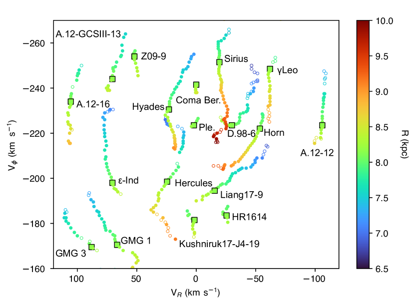
Figure 5: The $V_{R}$-$V_{\phi}$ kinematic plane with the locations of detected moving groups shown as a function of radii. The locations of the peaks of the moving groups are shown between radii of 6.5 kpc and 10.0 kpc with radius represented by color. The filled and empty circles represent those peaks with $P_{\mathrm{MC}}$ $\geq 0.8$ and $<0.8$, respectively. The green square points are the locations of the moving groups in the solar neighborhood region ($8.05<R<8.25$ kpc).

3 Results

Using Gaia DR3, we performed the wavelet transformation on the $V_{R}-V_{\phi}$ kinematic plane. We first binned the Gaia data into 600 bins of size 0.5 km s^-1 (in both dimensions; shown in Figure 1a). Then we used scales of $j=$ 2, 3, 4, and 5 (shown in Figure 3) for our WT. These scales allow us to detect structures in the histogram with sizes between $\Delta\times 2^{j}$ and $\Delta\times 2^{j+1}$ where $\Delta$ is the bin size (0.5 km s^-1). Since most of the stellar moving group structures have sizes of $\sim 10$ km s^-1, we used the $j=4$ scale for this analysis which corresponds to structures with sizes between 8 and 16 km s^-1. At smaller scales (Figure 3b) some of the classical moving groups (e.g. Hyades, Coma Berenices, Sirius) break into multiple components, and at larger scales (Figure 3) the groups merge together. While some of the small-scale features are interesting to explore in future works, the goal of this work is to compare with the existing studies of moving groups, so we will focus on the $j=4$ scale below.

3.1 Detected Moving Groups in the Solar Neighborhood

From the $j=4$ WT image, we are able to detect 47 moving groups listed in Table 1. Figure 1 shows the 2D histogram (Panel a) as well as the resultant wavelet coefficients and extrema (Panel b). Both panels show the locations of significant maxima as red crosses, while Panel b also shows significant minima as blue crosses. The identified moving groups are also shown in Figure 4 which shows only the overdensities with their corresponding ID number (column 1 in Table 1). The purple and green shaded regions in Figure 1b show the positive and negative wavelet coefficients, respectively. While our results for DR3 are in general very consistent with DR2 (shown in Figure 1c), the most significant differences arise from the restriction on the minimum number of stars for a detected maximum. As discussed above, at least 3 stars are required for relative maxima, and 4 stars are required for relative minima in order for consistent significance determination. This cutoff was not implemented in previous works, and for easier comparison with R18, it is disabled in our analysis of the DR2 data below.

We are able to detect 15 candidate overdensities in addition to finding 5 previously detected groups that were not detected in R18: Kushniruk17-J4-19 (Kushniruk et al., 2017), HR1614, Zhao09-9 (Zhao et al., 2009), Bobylev16-23 (Bobylev & Bajkova, 2016), and Antoja12-19 (Antoja et al., 2012). Our 15 candidate groups are numbered with a “DR3G” (Data Release 3 Group) prefix in Table 1. Of our 15 candidate groups discovered, 6 meet the confidence level criteria (CL $\geq 2$), 7 meet the Monte Carlo criteria ($P_{\mathrm{MC}}>0.8$), and 3 groups meet both criteria (Groups 25, 26, and 31 in Table 1). Group 25 lies within Arcturus, and Groups 26 and 31 are in regions without much substructure at low $V_{R}$. These groups are circled in Figure 1a and b.

To compare our wavelet method with previous works, we have reproduced the steps of R18. Following their selection of Gaia DR2 data, our code is able to detect all of the top 24 groups listed in their Table 3. We also find 11 of the remaining 20 groups (all of which were new detections not matching any previously known moving group). In addition to the groups found in R18, our wavelet code detects six previously identified groups: Kushniruk17-J5-2, Kushniruk17-J4-19 (Kushniruk et al., 2017), Dehnen98-11 (Dehnen, 1998), HR1614, Zhao09-9 (Zhao et al., 2009), Antoja12-19, and Antoja12-15 (Antoja et al., 2012).

There are also 33 detected overdensities that don’t overlap with any of the groups listed in Table 3 or C.1 in R18, however only 3 of these meet the confidence level and Monte Carlo criteria (Groups 30, 39, and 49 in Table 3). Groups 39 and 49 use fewer than 3 stars to calculate the wavelet coefficient which is below our cutoff in the DR3 data. Group 30 is detected in the DR3 data as well (Group 25 in Table 1) slightly shifted but it remains significant and robust against the Monte Carlo simulations.

	Name	$r_{\mathrm{min}}$ (kpc)	$r_{\mathrm{max}}$ (kpc)	Extent (kpc)
3	Sirius	7.45	10.00*	2.55
5	Hercules	6.95	9.25	2.30
1	Hyades	7.20	9.05	1.85
7	Dehnen98-6	6.75	8.35	1.60
10	Liang17-9	6.85	8.40	1.55
6	Dehnen98-14 (Horn)	7.85	9.30	1.45
9	$\epsilon$Ind	7.00	8.40	1.40
14	Antoja12-12	7.30	8.65	1.35
13	GMG 1	7.25	8.55	1.30
17	Antoja12-16	7.65	8.85	1.20
8	$\gamma$Leo	7.85	9.05	1.20
12	Antoja12-GCSIII-13	7.55	8.50	0.95
19	GMG 3	7.40	8.25	0.85
11	Kushniruk17-J4-19	7.95	8.50	0.55
20	Zhao09-9	8.00	8.40	0.40
4	Coma Berenices	8.15	8.50	0.35
16	HR1614	7.95	8.25	0.30
2	Pleades	8.00	8.20	0.20

Table 2: Radial extent of the moving groups shown in Figure 5. The first column lists the ID corresponding to the groups in Table 1. Note that we found that Sirius extends to the maximum radius of 10 kpc, so it could extend further outwards.

3.2 Moving Groups Across the Disk

One of the most valuable aspects of automated WTs is the ability to quickly and easily detect overdensities and underdensities for an arbitrary dataset. We have used this to analyze different bins of Gaia DR3 data to track moving groups throughout Galactocentric radius. We selected 70 radial bins centered on $R$ ranging from 6.5 to 10 kpc with a bin size of 0.2 kpc.

For each bin, we run the WT and determine the locations and significance of each overdensity. By plotting each detected peak on the kinematic plane, we can track the evolution of the moving groups throughout the Galactic disk. This is shown in Figure 5 (some extraneous detections not associated with a continuous stream have been removed). Each dot is a detected peak colored by its Galactocentric radius. The moving groups in the SN are shown as square markers and are labelled. Here we can clearly see that many of the detected moving groups extend $\gtrsim$1 kpc radially throughout the Galactic disk. The tracked groups with their radial extents are listed in Table 2. We also note that there are four groups with very limited radial extent ($<0.5$ kpc): Coma Berenices, HR1614, Pleiades, and Zhao09-9. A discussion of the differences between these and the radially extended groups is included in Section 4.

3.2.1 Shapes of Moving Groups in the Kinematic Plane

In addition to simply detecting the peaks of overdensities, the WT evaluates the wavelet coefficients across the entire image (shown as green and purple shaded regions in Figure 1b and c). We can then look at the shape of the moving groups in kinematic space by plotting contours of constant wavelet coefficient. We have also performed this analysis as a function of radius and the results are shown in Figure 6. Note that while the contour levels are consistent across radius within a single group (e.g. all contours for the Hercules group are 10% of the maximum wavelet coefficient at each radius), the contour levels vary from group to group (e.g. the contours for Sirius are at the 40% level whereas the contours for Hyades are at the 90% level). This allows for optimum visualization of groups with different wavelet coefficient values, however this means that the relative size between groups in this figure does not have meaning. The main purpose of this figure is to show how the kinematics of individual groups changes with radius.

For example, as we progress towards the Galactic center, we can see that Hercules covers a larger portion of the kinematic plane. Therefore, at smaller radii, the percentage of stars in the Hercules stream increases. Converesely, as we progress towards the outer disk, Hercules tends to disappear. We see a similar but inverse trend with Sirius. At smaller Galactocentric radii, the contours around Sirius shrink and eventually vanish, but as we progress past the SN and beyond into the outer disk, Sirius grows to cover a significant portion of the kinematic plane.

4 Discussion

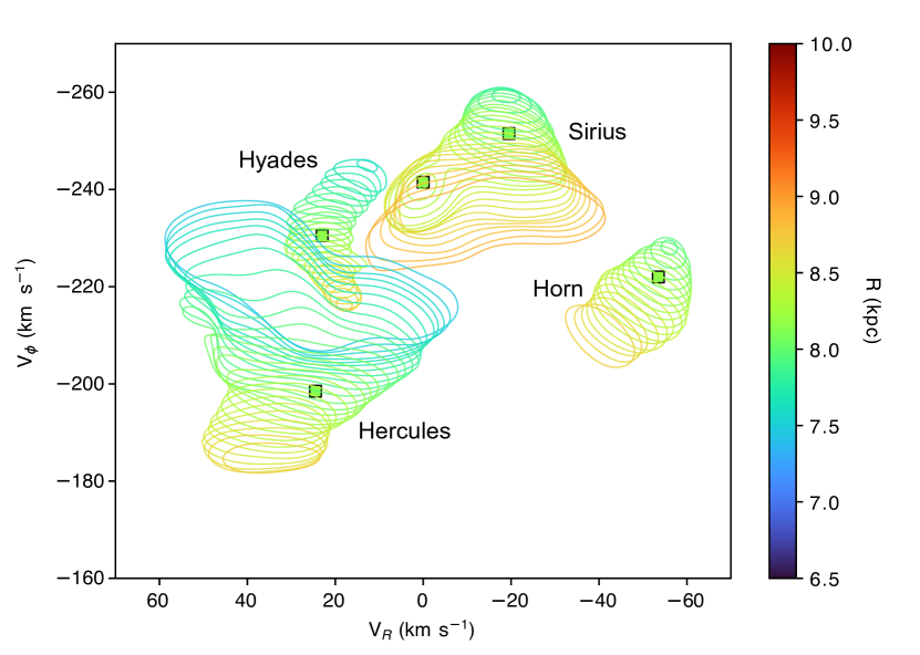
Figure 6: As in Fig 5, except each moving group is designated by contours of constant wavelet coefficient. Note that the axis limits are different from Figure 5. This allows us to see how the shapes of the groups vary as a function of radius. Note only four groups are displayed here to maintain clarity.

Our WT code, MGwave, performs 2D wavelet transformations with the goal of detecting statistically significant circular overdensities and underdensities at varying scales. This is distinct from many recent WT analyses of the SN kinematic plane. R18 don’t include a minimum star count cutoff and thus detect many more fringe overdensities that we consider not significant against Poisson noise. Yang et al. (2021) use a bivariate WT to detect features in the $V$ vs $\sqrt{U^{2}+2V^{2}}$ space and they utilize a Gaussian mixture model with Monte Carlo sampling to generate a smooth background distribution to compare against. Bernet et al. (2022) explore the $V_{R}-V_{\phi}$ plane by performing a one-dimensional WT on slices in $V_{R}$. By linking peaks in the 1D WT with neighboring $V_{R}$ bins, they detect arches in the kinematic plane analogous to those found in R18.

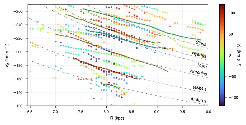
Figure 7: The variation of $V_{\phi}$ with $R$. Each point is a detected overdensity in the kinematic plane colored by $V_{R}$. The solar neighborhood is shown with a vertical dashed line at 8.15 kpc. The continuous streams associated with Sirius, Hyades, the Horn, Hercules, GMG 1, and Arcturus are shown as connected points and curves of constant angular momentum are shown as dashed lines. Note that only those points with $P_{\mathrm{MC}}\geq 0.8$ are shown.

While previous works have analyzed moving groups through radius (e.g. R18; Antoja et al. 2018; Fragkoudi et al. 2019; Bernet et al. 2022), they have focused on the variation in the locations of the peak overdensities (e.g. Figures 5, 7). Our Figure 6 shows that the WT can provide much richer information than simply the location of the extrema. The contours of these groups and how they evolve with radius and azimuth can be informative on the properties of the non-axisymmetric features of the Galactic disc. Because many of these groups are so extended in radius, we know that they are not local, transient structures, but large-scale features of the MW disk. Their extent indicates that these moving groups are likely formed through the gravitational effects of the MW’s non-axisymmetric features.

The MW’s bar and spiral arms and their associated resonances have long been used to explain the origin of moving groups. The specific resonances that are able to form the groups depend on the bar model (e.g. Hercules can be formed by the outer Lindblad resonance of a short bar or by the corotation resonance of a longer bar). However, recent works seem to indicate that a long bar with pattern speed of $\sim$40 km s^-1 kpc^-1 is consistent with both direct observations (Clarke et al., 2019; Sanders et al., 2019) and can explain many of the moving groups that we detect in the SN (Monari et al., 2019; D’Onghia & L. Aguerri, 2020; Trick et al., 2021). D’Onghia & L. Aguerri (2020) proposed a model with a bar of length 4.5 kpc and pattern speed of 40 km s^-1 kpc^-1and showed that Hercules is reproduced by stars at the corotation resonance with the bar. In this scenario Hercules’ stars are librating around the bar’s Lagrange points L4/L5 thus leading to a stream of stars with coherent velocity (slower than the sun) in the SN (see their Figure 4). As shown in our Figures 5 and 6, Hercules is extended in radius around the SN. Moreover, Figure 6 shows that Hercules grows to cover a significant portion of the kinematic plane for $R<R_{\odot}$. In the models of D’Onghia & L. Aguerri (2020), the bar’s corotation radius is around 6 kpc, so if the stars of Hercules are formed through trapping at corotation, we would expect Hercules to become more significant at smaller radii, consistent with the data.

The model of a long bar presented in Monari et al. (2019) also shows that five regions of in the kinematic plane correspond to resonances with the bar. To compare with this work, we performed the WT on the Gaia DR3 data transformed into $U,V,W$ coordinates. Figure 8 shows this WT image and the corresponding overdensities numbered by their corresponding group in Table 1. The colored lines show the locations of the resonances from the long bar model of Monari et al. (2019): red, blue, and purple correspond to the 2:1 (OLR), 4:1 (outer ultra-harmonic resonance, OUH), and 6:1 resonances, while the green and yellow lines mark the corotation resonance. In addition to Hercules being stars at corotation with the bar, the authors find that the Hat aligns with OLR, Sirius with the OUH, and the Horn with the 6:1 resonances. All of these groups are shown in our Figure 5 and are still prominent across Galactocentric radius. Moreover, Figure 6 shows Sirius becoming more prominent at larger radii (opposite of Hercules). For a bar with a pattern speed of $\sim$40 km s^-1 kpc^-1, the location of the OUH is at 8.5-9 kpc (D’Onghia & L. Aguerri, 2020). Therefore, we expect more stars comprising Sirius as we look towards the outer Galactic disk, which is shown in the data.

There are several other groups that we detect with significant radial extent, many of which are also identified being in resonance with the bar (Monari et al., 2019) shown in Figure 8. Antoja12-16, Antoja12-GCSIII-13, $\gamma$Leo, Zhao09-9, and possibly Antoja12-12 fall on the OUH resonance along with Sirius. Dehnen98-6 aligns well with the 6:1 resonance along with the Horn. Finally, $\epsilon$Ind and Hercules and Liang17-9 are all at corotation.

This leaves four groups with radial extent greater than 0.5 kpc unaccounted for: the Hyades, GMG 1, GMG 3, and Kushniruk17-J4-19. While Hyades doesn’t seem to have formed through any known bar resonance, works focusing on the kinematic signatures of spiral arm resonances have been able to reproduce Hyades along with several other features of the SN kinematic plane (Michtchenko et al. 2018; Barros et al. 2020; including low $V_{\phi}$ features like GMG 1,3, and Kushniruk17-J4-19). However, these models predict that the moving groups are significantly extended in $\phi$, and less extended in $R$. Further work will be required to constrain the groups in $\phi$ to test this theory. Additionally, our detection of Hyades throughout a large range of Galactocentric radii could be simply the detection of the main mode in each neighborhood. We expect a smooth evolution of $V_{\phi}$ across radius with stars being mostly on circular orbits. Therefore, while the main mode might be identified as Hyades locally, at different radii, the detected peak could simply be the bulk motion of the disk. This would also explain why it is unique in its double slope in $V_{R}$ in Figure 1 (discussed further below).

There are also five groups detected that have small radial extent ($<0.5$ kpc): Coma Berenices, the Pleiades, HR1614, Boblyev16-23, and DR3G-21 (which was briefly discussed above). It has been shown previously that Coma Berenices and the Pleiades are open clusters (e.g. Odenkirchen et al., 1998; Tang et al., 2018; Heyl et al., 2022). Figure 5 and Table 2 corroborates this result by showing that these objects are detected only locally within the SN. While HR1614 has long been considered an open cluster (e.g. Feltzing & Holmberg, 2000; De Silva et al., 2007) recent works suggest that its metallicity spread matches that of the MW disk population (Kushniruk et al., 2020). Further investigation is required to unravel the true origin of HR1614.

We apply our MGwave code to Gaia DR3. Figure 7 shows the azimuthal velocity of the known moving groups of the SN displayed as a function of Galactocentric radius. Each moving groups is colored by radial velocity. Bernet et al. (2022) showed the same plot but using a 1D WT technique applied to the previous Gaia data release (eDR3). The authors found that all major groups deviate from the predicted $V_{\phi}\propto R^{-1}$. Note that our results obtained with DR3 seem to confirm a deviation from the constant angular momentum curve (dashed line) for most of the known moving groups, with the exception of GMG 1. This general outcome is not surprising as the constant angular momentum curve is expected for small radial oscillations of the stars, within the epicycle approximation. Therefore, a deviation is expected for highly eccentric stars. Additionally, even with the improved data of Gaia DR3, we are unable to trace our groups much inwards of $R\sim 7$ kpc while Bernet et al. (2022) find groups extending down to 5 kpc. This discrepancy could be due to the difference in the wavelet method (searching for arches vs. search for circular features). However it is also clear that the data become less accurate at these radii. While the WT is able to detect significant overdensities even at these small radii, many of them have small $P_{\mathrm{MC}}$ values indicating that they are not robust detections against the Gaia errors (see Section 2.4).

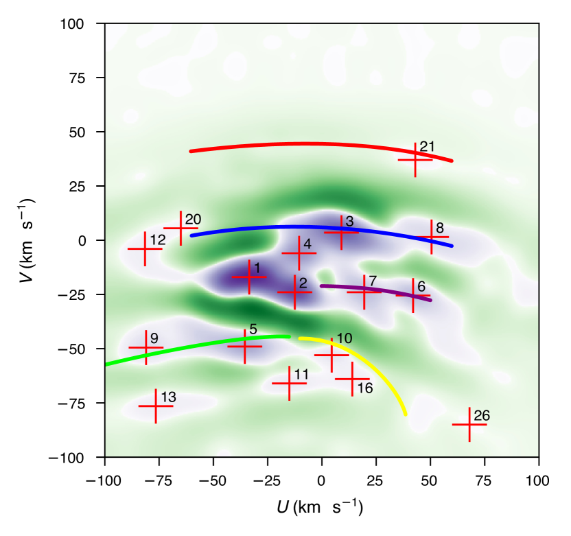
Figure 8: The $j=4$ wavelet transformed image of the solar neighborhood in $U,V,W$ coordinates. Coordinates were transformed from Gaia DR3 source data to the Astropy default Galactic coordinate system (in the cartesian representation). The overdensities are numbered as in Figure 4. Overlaid are the bar resonance locations from Monari et al. (2019) (c.f. their Figure 9). “The green and yellow lines correspond to the corotation, the red line to the 2:1 (OLR) resonance for the m = 2 mode, … the blue line to the 4:1 resonance of the m = 4 mode, and the purple line to the 6:1 resonance of the m = 6 mode.”

Our Figure 5 shows that there is also a significant variation in $V_{R}$ with $R$. Notably that most groups have a shift in $V_{R}$ as they move in radius, however the direction of this shift (the slope of the connected points in Figure 5) can be positive, negative, or both. Four groups have strong positive slopes (e.g. Liang17-9, Dehnen98-6, the Horn, and the majority of Hercules) in which they move to larger $V_{R}$ at higher radii, and three have strong negative slopes (GMG 3, GMG 1, and Kushniruk17-J4-19) with smaller $V_{R}$ at higher radii. Several other groups have slight slopes in either direction, or multiple slopes at different radii. Notably, Hyades moves to larger $V_{R}$ until it reaches the solar neighborhood at which point it decreases again, and Hercules, Sirius, and Dehnhn98-6 exhibit breaks or strong variations in the slope throughout radius.

For the positive slope groups, the inner portion (smaller $R$) has an inward velocity relative to the centroid, while the outer portion (larger $R$) has an outward velocity. This will inevitably lead to the group spreading out and possibly breaking apart. Consequently, negative slope groups exhibit the opposite trend and therefore are condensing. These two different behaviors of groups could possibly indicate environmental effects operating at different radii like tidal effects, but further analysis of the data in comparison with simulations is required to fully explore the possible causes of these slopes.

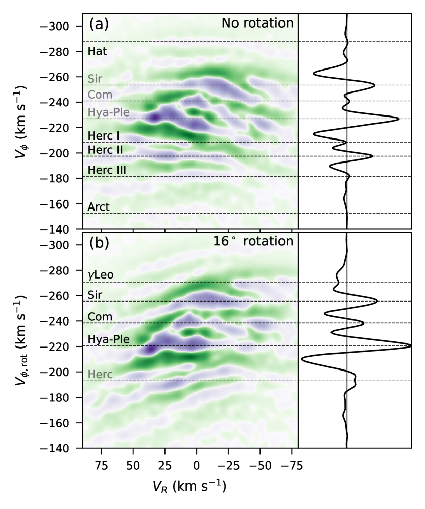
Figure 9: The wavelet plane and its histogram along $V_{\phi}$ for $j=3$, structures of size 4-8 km s^-1. In the top panels, the wavelet plane is identical to that shown in Figure 3, however on the bottom panels, the plane has been rotated by 16^∘ counter-clockwise. As done in Antoja et al. (2008), this is to better align the Hyades-Pleiades, Coma Berenices, and Sirius overdensities with the $x$-axis. However, as shown in the top panel, there are several structures (Hercules, the Hat, and Arcturus) which do not match this distinctive rotation. The line plots on the right show the sums of wavelet coefficients across all $V_{R}$ as a function of $V_{\phi}$. These panels show that the Hyades-Pleiades, Coma Berenices, and Sirius overdensities are stronger and more prominent after a 16^∘ rotation of the plane, whereas Hercules, the Hat, and Arcturus are stronger without the rotation.

Looking at the larger structure of the WT images, previous works (e.g. Skuljan et al., 1999; Antoja et al., 2008) have noted several distinct kinematic branches visible in the $V_{R}-V_{\phi}$ plane. Note that these features have been explored at smaller scales that those discussed throughout most of this paper. In the following paragraphs we will be referencing our results from the WT with scale $j=3$. Antoja et al. (2008) found that these branches are inclined at an angle of $\sim$16^∘ and the four most prominent are aligned with the Hercules, Hyades/Pleiades, Coma Berenices, and Sirius groups. These branches are still clearly visible in our data (see Figure 1c), however thanks to Gaia’s immense volume of data, we can now view these structures across larger ranges of $V_{R}$. Gaia Collaboration et al. (2018) and R18 extended these branches into arches, most of which follow constant kinetic energy. In contrast to the uniformly inclined branches found in Antoja et al. (2008), Gaia’s increased data has elongated and straightened out many of these structures. However, as discussed in R18, several of the arches are still inclined to one side; notably their A5 and A7 corresponding to Hyades/Pleiades and Coma Berenices. Several models have shown that these arches of constant kinetic energy can be formed through phase mixing (Minchev et al. 2009; Gómez et al. 2012; R18) which could play a role in the formation of the moving groups as well. However further investigation is required to constrain this paradigm.

In this study we have returned to the method of Antoja et al. (2008) of summing the wavelet transformed image along $V_{R}$ to obtain a histogram as a function of $V_{\phi}$. We have explored this histogram both with and without the 16^∘ rotation that was performed in Antoja et al. (2008). These results can be seen in Figure 9 (Panels (a) show the results without rotation and Panels (b) include the 16^∘ rotation). With the increased volume of data provided by Gaia, we can see that, while the Hyades/Pleiades, Coma Berenices, and Sirius branches do still appear inclined (and we see $\gamma$Leo appear in the rotated histogram as well), there are several other structures that do not follow this trend. Most dramatically, we see three strong peaks in the non-rotated histogram corresponding to various components of Hercules. By looking at the wavelet plane, the horizontal alignment of these branches is clearly visible, while in the rotated plane (bottom panels) Hercules becomes muddled. We also see slight peaks in the non-rotated histogram corresponding to the Hat at very high $V_{\phi}$, and Arcturus at very low $V_{\phi}$. While some of the these tilted features have been reproduced in past simulations (e.g. Antoja et al., 2009; Hunt et al., 2018; Barros et al., 2020), further modeling is required to determine their source specifically in the context of a long, slow bar.

5 Conclusions

The wavelet transform is an invaluable tool for precise, quantitative analysis of images. Our new code, MGwave, is an open-source Python module for performing wavelet transformations on 2D images while detecting extrema and determining their significance. Additionally, we have implemented Monte Carlo sampling to propagate errors and uncertainties through to the wavelet extrema detections. MGwave is able to reproduce the findings of R18 (using Gaia DR2 data) and improves upon previous codes by detecting underdensities in addition to overdensities and implementing a minimum $n$ cutoff in the significance calculation.

We performed the WT on Gaia DR3 data to detect moving groups in the kinematic plane ($V_{R}-V_{\phi}$) of the solar neighborhood (Figure 1). With the improved data, we have several main conclusions:

• We have detected three new, statistically significant candidate moving groups: one within Arcturus, and two in regions without much substructure at low $V_{R}$.

• We have been able to perform the WT on different regions within the MW disk. Exploring the structure of the kinematic plane in sections of the disk ranging in Galactocentric radius from 6.5 to 10 kpc, we find that the majority of the moving groups detected within the SN are radially extended (Figure 5). The elongation of these groups indicate that they are dynamical structures possibly outcome by the effects of resonances of the MW’s non-axisymmetric features.

• By mapping contours in wavelet space, we can track the variation in the kinematic shape of these groups through radius (Figure 6). We find Hercules becoming more prominent towards the galactic center, in agreement with the models of D’Onghia & L. Aguerri (2020) that predicted that Hercules is comprised of stars at corotation with the bar.

• Mapping WT contours also reveals an opposite trend for Sirius, it gets more prominent towards the outer disc. This is consistent with Sirius being in resonance with the OUH located outside the solar radius (Monari et al., 2019).

Gaia DR3 has greatly expanded our view of the MW. By looking at the kinematics of moving groups throughout a significant portion of the disk, we can unravel many of the mysteries of the MW’s non-axisymmetric features and their associated resonances.

Data Availability

The data underlying this article will be shared on reasonable request to the corresponding author.

	$V_{R}$	$V_{\phi}$	Name	CL	$P_{\mathrm{MC}}$	Wavelet	n	Stars
1	22.5	-236.0	Hyades	3	1.00	7.6596	394	130,982
2	1.5	-228.5	Pleiades	3	1.00	5.6223	438	162,864
3	-20.0	-256.5	Sirius	3	1.00	4.9166	376	87,694
4	-1.0	-247.0	Coma Berenices	3	1.00	3.0033	538	130,122
5	24.0	-203.5	Hercules II	3	1.00	2.0458	157	58,368
6	-54.0	-227.5	Dehnen98-14	3	1.00	1.5060	141	44,723
7	-31.0	-228.5	Dehnen98-6	3	1.00	1.2256	293	90,548
8	-64.0	-253.5	$\gamma$Leo	3	1.00	0.5601	68	20,072
9	70.5	-203.0	$\epsilon$Ind	3	1.00	0.5349	43	17,400
10	-53.0	-258.0	Kushniruk17-J5-2*	3	0.93	0.4607	112	23,082
11	-16.5	-199.5	Liang17-9	3	1.00	0.2771	109	38,112
12	70.0	-250.5	Antoja12-GCSIII-13	3	1.00	0.1807	24	9,614
13	64.0	-239.0	Dehnen98-11*	3	0.99	0.1570	61	17,261
14	66.0	-175.5	GMG 1	3	1.00	0.1473	20	9,255
15	-7.0	-187.5	GMG 2	3	1.00	0.1293	102	31,186
16	-68.0	-210.0	Unknown	3	0.47	0.1248	54	22,073
17	-108.5	-229.0	Antoja12-12	3	1.00	0.1208	11	3,764
18	106.5	-239.5	Antoja12-16	3	1.00	0.1111	6	2,233
19	2.5	-186.0	Kushniruk17-J4-19*	3	0.60	0.1077	76	33,118
20	47.0	-178.0	Arifyanto05	3	0.86	0.0898	34	14,832
21	88.5	-174.5	GMG 3	3	0.98	0.0708	6	3,953
22	36.0	-153.5	$\eta$Cep	3	0.93	0.0602	12	5,041
23	-51.0	-291.0	GMG 4	3	1.00	0.0529	6	1,345
24	-28.5	-189.0	HR1614*	1	0.81	0.0314	59	20,115
25	-26.0	-150.0	Antoja12-17	3	1.00	0.0311	7	3,087
26	48.0	-259.5	Zhao09-9*	0	1.00	0.0292	71	14,006
27	-56.0	-176.0	GMG 5	3	1.00	0.0276	14	5,037
28	106.0	-272.5	GMG 6	3	0.99	0.0254	1	318
29	-134.0	-225.5	GMG 7	3	1.00	0.0173	1	535
30	2.5	-157.5	Unknown	2	0.98	0.0170	14	6,182
31	-14.0	-153.0	Unknown	1	0.37	0.0159	17	4,305
32	129.0	-237.5	GMG 8	3	1.00	0.0159	1	496
33	112.5	-155.0	Unknown	3	0.68	0.0123	3	1,078
34	-88.0	-233.0	Unknown	0	1.00	0.0120	40	10,436
35	73.0	-282.0	GMG 11	2	1.00	0.0112	4	770
36	-108.0	-152.0	GMG 12	3	0.99	0.0106	1	345
37	125.5	-175.0	GMG 14	3	1.00	0.0104	3	654
38	-78.0	-130.5	GMG 13	2	0.97	0.0101	4	500
39	83.5	-143.5	Unknown	2	0.97	0.0095	2	1,285
40	-79.0	-166.5	Unknown	1	0.99	0.0092	8	1,671
41	-1.0	-120.0	GMG 17	1	0.97	0.0090	6	709
42	-24.0	-91.0	GMG 16	3	1.00	0.0085	1	219
43	71.0	-142.5	Unknown	2	0.49	0.0082	3	1,431
44	-59.0	-138.0	Unknown	3	0.44	0.0070	1	1,019
45	-39.0	-139.0	Antoja12-19*	1	0.90	0.0067	6	1,568
46	13.5	-82.0	GMG 19	3	0.85	0.0067	1	158
47	122.0	-202.5	GMG 20	1	0.96	0.0065	5	837
48	-96.5	-158.5	Unknown	1	0.78	0.0063	4	636
49	-66.5	-108.0	Unknown	3	0.97	0.0061	1	298
50	-42.5	-119.0	GMG 22	1	1.00	0.0040	2	591
51	125.0	-146.5	Unknown	1	0.49	0.0037	2	472
52	-26.5	-107.0	Unknown	1	0.83	0.0033	1	384
53	137.5	-164.5	Unknown	1	0.66	0.0028	1	381
54	-98.5	-135.0	Unknown	1	0.88	0.0028	1	304
55	136.5	-138.0	Unknown	1	0.93	0.0025	2	248
56	-127.5	-184.5	Unknown	0	0.89	0.0022	2	486
57	-70.5	-174.0	Antoja12-15*	0	0.42	0.0022	6	3,081
58	109.0	-118.5	Unknown	1	0.60	0.0021	1	203
59	140.0	-83.0	Unknown	1	0.96	0.0020	1	42

Table 3: Moving groups detected using our new wavelet transform on Gaia DR2 data. Compare with those found in R18. Groups marked with an asterisk (*) are those that have been previously discovered but were not present in the wavelet analysis of R18. Bold lines are groups newly discovered in this work. Columns 5-9 list the output of our analysis: CL denotes the confidence level that a given group is not due to Poisson noise (see Section 2.3); $P_{\mathrm{MC}}$ gives the percentage of Monte Carlo simulations in which the peak appeared when varying the stellar velocities within Gaia errors (see Section 2.4); Wavelet gives the magnitude of the wavelet coefficient at the peak; n lists the number of stars used in computing the wavelet coefficient; Stars lists the number of stars in a region of kinematic space around the peak corresponding to the scale of the wavelet transformation performed (in this case within a circle of radius 16 km s^-1).

60	50.5	-106.0	Unknown	1	0.54	0.0017	1	260
61	-47.5	-88.0	Unknown	0	0.28	0.0016	2	180
62	72.5	-78.0	Unknown	1	0.22	0.0015	1	113
63	-109.0	-340.0	GMG 27	1	0.98	0.0012	1	6
64	47.0	-342.0	GMG 26	0	0.73	0.0012	2	13
65	129.5	-125.0	Unknown	1	0.87	0.0011	1	200
66	-114.5	-320.0	Unknown	1	0.96	0.0011	1	8
67	-35.5	-74.0	Unknown	0	0.75	0.0011	2	139
68	80.0	-116.5	Unknown	0	0.58	0.0010	3	306
69	-25.0	-122.0	Unknown	0	0.88	0.0010	3	837
70	-24.0	-326.5	Unknown	0	0.69	-0.0000	1	36
71	-62.0	-153.0	Unknown	0	0.21	-0.0012	5	1,823
72	-102.5	-183.5	Unknown	0	0.97	-0.0018	7	1,449
73	-56.5	-161.5	Unknown	0	0.25	-0.0022	8	2,953
74	-113.5	-199.0	Unknown	0	0.85	-0.0026	8	1,330

Table 4: Gaia DR2 moving group detections continued.

References

- Alves et al. (2020) Alves J., et al., 2020, Nature, 578, 237
- Antoja et al. (2008) Antoja T., Figueras F., Fernández D., Torra J., 2008, A&A, 490, 135
- Antoja et al. (2009) Antoja T., Valenzuela O., Pichardo B., Moreno E., Figueras F., Fernández D., 2009, ApJ Letters, 700, L78
- Antoja et al. (2012) Antoja T., et al., 2012, MNRAS, 426, L1
- Antoja et al. (2018) Antoja T., et al., 2018, Nature, 561, 360
- Asano et al. (2020) Asano T., Fujii M. S., Baba J., Bédorf J., Sellentin E., Portegies Zwart S., 2020, MNRAS, 499, 2416
- Astropy Collaboration et al. (2013) Astropy Collaboration et al., 2013, A&A, 558, A33
- Astropy Collaboration et al. (2018) Astropy Collaboration et al., 2018, AJ, 156, 123
- Astropy Collaboration et al. (2022) Astropy Collaboration et al., 2022, apj, 935, 167
- Bailer-Jones et al. (2020) Bailer-Jones C., Rybizki J., Fouesneau M., Demleitner M., Andrae R., 2020, Gaia eDR3 lite distances subset, VO resource provided by the GAVO Data Center, http://dc.zah.uni-heidelberg.de/tableinfo/gedr3dist.litewithdist
- Bailer-Jones et al. (2021) Bailer-Jones C. A. L., Rybizki J., Fouesneau M., Demleitner M., Andrae R., 2021, AJ, 161, 147
- Barros et al. (2020) Barros D. A., Pérez-Villegas A., Lépine J. R. D., Michtchenko T. A., Vieira R. S. S., 2020, ApJ, 888, 75
- Bernet et al. (2022) Bernet M., Ramos P., Antoja T., Famaey B., Monari G., Al Kazwini H., Romero-Gómez M., 2022, arXiv e-prints, p. arXiv:2206.01216
- Bobylev & Bajkova (2016) Bobylev V. V., Bajkova A. T., 2016, Astronomy Letters, 42, 90
- Clarke et al. (2019) Clarke J. P., Wegg C., Gerhard O., Smith L. C., Lucas P. W., Wylie S. M., 2019, MNRAS, 489, 3519
- Craig et al. (2021) Craig P., Chakrabarti S., Newberg H., Quillen A., 2021, MNRAS, 505, 2561
- D’Onghia & L. Aguerri (2020) D’Onghia E., L. Aguerri J. A., 2020, ApJ, 890, 117
- Da Rocha & Mendes de Oliveira (2005) Da Rocha C., Mendes de Oliveira C., 2005, MNRAS, 364, 1069
- Da Rocha et al. (2008) Da Rocha C., Ziegler B. L., Mendes de Oliveira C., 2008, MNRAS, 388, 1433
- De Silva et al. (2007) De Silva G. M., Freeman K. C., Bland-Hawthorn J., Asplund M., Bessell M. S., 2007, AJ, 133, 694
- Debattista et al. (2002) Debattista V. P., Gerhard O., Sevenster M. N., 2002, MNRAS, 334, 355
- Dehnen (1998) Dehnen W., 1998, AJ, 115, 2384
- Dehnen (2000) Dehnen W., 2000, AJ, 119, 800
- Eggen (1996) Eggen O. J., 1996, AJ, 112, 1595
- Einasto et al. (2011) Einasto J., et al., 2011, A&A, 531, A75
- Feltzing & Holmberg (2000) Feltzing S., Holmberg J., 2000, A&A, 357, 153
- Fragkoudi et al. (2019) Fragkoudi F., et al., 2019, MNRAS, 488, 3324
- Fujii et al. (2019) Fujii M. S., Bédorf J., Baba J., Portegies Zwart S., 2019, MNRAS, 482, 1983
- Gaia Collaboration et al. (2016) Gaia Collaboration et al., 2016, A&A, 595, A1
- Gaia Collaboration et al. (2018) Gaia Collaboration et al., 2018, A&A, 616, A11
- Gaia Collaboration et al. (2022a) Gaia Collaboration Vallenari A., Brown A., Prusti T., 2022a, A&A
- Gaia Collaboration et al. (2022b) Gaia Collaboration Drimmel R., Romero-Gómez M., Chemin L., Ramos P., Poggio E., Ripepi V., 2022b, arXiv e-prints, p. arXiv:2206.06207
- Girardi et al. (1997) Girardi M., Escalera E., Fadda D., Giuricin G., Mardirossian F., Mezzetti M., 1997, ApJ, 482, 41
- Gómez et al. (2012) Gómez F. A., Minchev I., Villalobos Á., O’Shea B. W., Williams M. E. K., 2012, MNRAS, 419, 2163
- Hergt et al. (2017) Hergt L., Amara A., Brandenberger R., Kacprzak T., Réfrégier A., 2017, J. Cosmology Astropart. Phys., 2017, 004
- Heyl et al. (2022) Heyl J., Caiazzo I., Richer H. B., 2022, ApJ, 926, 132
- Hunt et al. (2018) Hunt J. A. S., Hong J., Bovy J., Kawata D., Grand R. J. J., 2018, MNRAS, 481, 3794
- Kushniruk et al. (2017) Kushniruk I., Schirmer T., Bensby T., 2017, A&A, 608, A73
- Kushniruk et al. (2020) Kushniruk I., Bensby T., Feltzing S., Sahlholdt C. L., Feuillet D., Casagrande L., 2020, A&A, 638, A154
- Liang et al. (2017) Liang X. L., Zhao J. K., Oswalt T. D., Chen Y. Q., Zhang L., Zhao G., 2017, ApJ, 844, 152
- Michtchenko et al. (2018) Michtchenko T. A., Lépine J. R. D., Pérez-Villegas A., Vieira R. S. S., Barros D. A., 2018, ApJ Letters, 863, L37
- Minchev et al. (2009) Minchev I., Quillen A. C., Williams M., Freeman K. C., Nordhaus J., Siebert A., Bienaymé O., 2009, MNRAS, 396, L56
- Monari et al. (2017) Monari G., Kawata D., Hunt J. A. S., Famaey B., 2017, MNRAS, 466, L113
- Monari et al. (2019) Monari G., Famaey B., Siebert A., Wegg C., Gerhard O., 2019, A&A, 626, A41
- Odenkirchen et al. (1998) Odenkirchen M., Soubiran C., Colin J., 1998, New Astron., 3, 583
- Pérez-Villegas et al. (2017) Pérez-Villegas A., Portail M., Wegg C., Gerhard O., 2017, ApJ Letters, 840, L2
- Price-Whelan (2018) Price-Whelan A., 2018, adrn/pyia: v0.2, doi:10.5281/zenodo.1228136, https://doi.org/10.5281/zenodo.1228136
- Quillen et al. (2011) Quillen A. C., Dougherty J., Bagley M. B., Minchev I., Comparetta J., 2011, MNRAS, 417, 762
- Ramos et al. (2018) Ramos P., Antoja T., Figueras F., 2018, A&A, 619, A72
- Reid et al. (2014) Reid M. J., et al., 2014, ApJ, 783, 130
- Reid et al. (2019) Reid M. J., et al., 2019, ApJ, 885, 131
- Rogers et al. (2016) Rogers K. K., Peiris H. V., Leistedt B., McEwen J. D., Pontzen A., 2016, MNRAS, 463, 2310
- Sanders et al. (2019) Sanders J. L., Smith L., Evans N. W., 2019, MNRAS, 488, 4552
- Sanz et al. (1999) Sanz J. L., Argüeso F., Cayón L., Martínez-González E., Barreiro R. B., Toffolatti L., 1999, MNRAS, 309, 672
- Schönrich et al. (2010) Schönrich R., Binney J., Dehnen W., 2010, MNRAS, 403, 1829
- Skuljan et al. (1999) Skuljan J., Hearnshaw J. B., Cottrell P. L., 1999, MNRAS, 308, 731
- Slezak et al. (1993) Slezak E., de Lapparent V., Bijaoui A., 1993, ApJ, 409, 517
- Starck & Murtagh (1994) Starck J.-L., Murtagh F., 1994, A&A, 288, 342
- Starck & Murtagh (2006) Starck J.-L., Murtagh F., 2006, Astronomical Image and Data Analysis (Astronomy and Astrophysics Library). Springer-Verlag, Berlin, Heidelberg
- Starck et al. (1998) Starck J.-L., Murtagh F., Bijaoui A., 1998, Image Processing and Data Analysis. The Multiscale Approach. Vol. 94, Cambridge University Press, doi:10.1017/CBO9780511564352
- Tang et al. (2018) Tang S.-Y., Chen W. P., Chiang P. S., Jose J., Herczeg G. J., Goldman B., 2018, ApJ, 862, 106
- Thulasidharan et al. (2021) Thulasidharan L., D’Onghia E., Poggio E., Drimmel R., Gallagher John S. I., Swiggum C., Benjamin R. A., Alves J., 2021, arXiv e-prints, p. arXiv:2112.08390
- Trick (2022) Trick W. H., 2022, MNRAS, 509, 844
- Trick et al. (2021) Trick W. H., Fragkoudi F., Hunt J. A. S., Mackereth J. T., White S. D. M., 2021, MNRAS, 500, 2645
- Waskom (2021) Waskom M. L., 2021, Journal of Open Source Software, 6, 3021
- Xia et al. (2015) Xia Q., Liu C., Xu Y., Mao S., Gao S., Hou Y., Jin G., Zhang Y., 2015, MNRAS, 447, 2367
- Yang et al. (2021) Yang Y., Zhao J., Zhang J., Ye X., Zhao G., 2021, ApJ, 922, 105
- Zhao et al. (2009) Zhao J., Zhao G., Chen Y., 2009, ApJ Letters, 692, L113
- Zhao et al. (2014) Zhao J. K., Zhao G., Chen Y. Q., Oswalt T. D., Tan K. F., Zhang Y., 2014, ApJ, 787, 31
- Zhao et al. (2015) Zhao J.-K., Zhao G., Chen Y.-Q., Tan K.-F., Gao M.-T., Yang M., Zhang Y., Hou Y.-H., 2015, Research in Astronomy and Astrophysics, 15, 1378
- van der Walt et al. (2014) van der Walt S., et al., 2014, arXiv e-prints, p. arXiv:1407.6245