Entanglement in phase-space distribution for an anisotropic harmonic oscillator in noncommutative space

Abstract

The bi-partite Gaussian state, corresponding to an anisotropic harmonic oscillator in a noncommutative space (NCS), is investigated with the help of Simon’s separability condition (generalized Peres-Horodecki criterion). It turns out that, to exhibit the entanglement between the noncommutative coordinates, the parameters (mass and frequency) have to satisfy a unique constraint equation.
We have considered the most general form of an anisotropic oscillator in NCS, with both spatial and momentum non-commutativity. The system is transformed to the usual commutative space (with usual Heisenberg algebra) by a well-known Bopp shift. The system is transformed into an equivalent simple system by a unitary transformation, keeping the intrinsic symplectic structure ($Sp(4,\mathbb{R})$) intact. Wigner quasiprobability distribution is constructed for the bipartite Gaussian state with the help of a Fourier transformation of the characteristic function. It is shown that the identification of the entangled degrees of freedom is possible by studying the Wigner quasiprobability distribution in phase space. We have shown that the coordinates are entangled only with the conjugate momentum corresponding to other coordinates.

I Introduction

There is a consensus that most of the theories of quantum gravity appear to predict departures from classical gravity only at energy scales on the order of $10^{19}$ GeV qg1 ; qg2 (By way of comparison, the LHC was designed to run at a maximum collision energy of $14$ TeV lhc ). At that energy scale, the space-time structure is believed to be deformed in such a manner that the usual notion of commutative space will be ceased csseased1 ; csseased2 . It is almost a Gospel that the fundamental concept of space-time is mostly compatible with quantum theory in noncommutative space (NCS) Witten ; Juan . Formalisms of Quantum theory in NCS have been successfully applied to various physical situations ncsho ; ncsosc ; ncstopics ; ncsfluid . For the reviews on NCS, one can see ncsreview1 ; ncsreview2 .
Perhaps, due to the present-day technological limitation of attainable energy, the unified quantum theory of gravity lacks any direct experimental evidence. Moreover, the huge gap between the required ($10^{19}$ GeV) and the currently achievable energy scales suggests that we have to wait a long to successfully perform quantum gravity (QG) experiments in the regime of present-day colliders. However, instead of building a larger collider, there are various suggestions for the passive experiments regarding the QG, with the help of interferometry gravitationalwave1 ; catstatedeformed1 ; catstatedeformed2 ; catstatedeformed3 , in particular with the utilization of Coherent states (CS), for which the maximum contrast in the interference pattern is achieved interfero1 . In the context of CS, the bipartite Gaussian states are particularly important for their frequent appearance in systems with small oscillations bipartitegaussian1 ; bipartitegaussian2 . For example, the vibration of the test mass (corresponding to the masses on which the interferometric mirrors are placed) under the effects of the tidal forces of gravitational waves, can be demonstrated by an anisotropic oscillator gravitationalwave1 ; gravitationalwave2 ; gravitationalwave3 ; gravitationalwave4 , which exhibits a bipartite Gaussian state, upon consideration in a two-dimensional noncommutative space entangledgaussian1 ; entangledgaussian2 ; entangledgaussian3 ; entangledgaussian4 .
The entanglement properties of the bipartite state, corresponding to the noncommutative spatial degrees of freedom, are the central theme of the present article. A general separability criterion for a bipartite Gaussian state was proposed in separability1 , which is a generalization for the continuous variable states, over the discrete qubits separability2 ; separability3 .
At first, using a Bopp’s shift in co-ordinates boppsshift1 ; boppsshift2 ; boppsshift3 ; boppsshift4 , we have transformed the Hamiltonian ($\hat{H}_{nc}$) of the anisotropic harmonic oscillator in noncommutative space, to the equivalent Hamiltonian ($\hat{H}_{c}$) in commutative space. The structure of the $\hat{H}_{c}$ is similar to the Hamiltonians corresponding to a charged particle moving in presence of an inhomogeneous magnetic field. One of the major computational difficulties in the construction of the CS structure of an anisotropic oscillator in a magnetic field lies in the diagonalization of the quadratic system, keeping the intrinsic symplectic structure intact. In this article, to construct a linear canonical transformation (the group $Sp(4,\mathbb{R})$) to reduce our Hamiltonian to a simplified representative one, we have revisited the formalisms stated in separability4 ; separability5 ; separability6 ; separability7 ; separability8 . The ground state of the anisotropic harmonic oscillator (AHO) turns out to be a bipartite Gaussian state. Utilizing Simon’s separability criterion separability1 , we have obtained the restrictions on the masses ($m_{1},m_{2}$) and the parameters ($\theta,\eta$) (minimal length) of the noncommutative coordinates and momentums, for which the CS is separable.
For an entangled state, the identification of the entangled degrees of freedom is not straightforward. With the help of the well-known Wigner quasiprobability distribution (WQD) wigner1 ; wigner2 ; wigner3 ; wigner4 ; wigner5 ; wigner6 , we have identified the coordinates, which are entangled. Since WQD is the Fourier transform of the expectation value of the characteristic function of the random variables, it offers a phase-space description of a quantum system. It is believed that one can conceptually identify where the quantum corrections enter a problem by comparing it with the classical version. However, philosophical debates in this regard are inevitable, which we shall avoid in our present article. Rather, we shall indulge ourselves in the computation of WQD for our problem, keeping in mind that, being entirely real, WQD simplifies both the calculation and the interpretation, of the results. In our case, the random variables are the co-ordinate $(\hat{x}_{1},\hat{x}_{2})$ and momentum $(\hat{p}_{1},\hat{p}_{2})$ operators in commutative space. The study of the WQD suggests that for the system under consideration (AHO in NCS) coordinate degrees of freedom are entangled with the conjugate momentum corresponding to another coordinate. In particular, $\hat{x}_{1}$ is entangled with $\hat{p}_{2}$ and $\hat{x}_{2}$ is entangled with $\hat{p}_{1}$.
The organization of the article is the following. First, we have briefly discussed the system under consideration. Then, we diagonalized the Hamiltonian, with the help of a $Sp(4,\mathbb{R})$ canonical transformation. Coherent states are formed from the annihilation operators. After that, Simon’s separability criterion is utilized to identify the constraints on the parameters, which can be used as an entanglement criterion for our system. The identification of the entangled degrees of freedom was performed with the help of the study of Wigner quasiprobability phase space distribution.

II Anisotropic harmonic oscillator in noncommutative space

We have studied the phenomenology of a two-dimensional anisotropic harmonic oscillator in noncommutative (NC) space, with both the configuration and momentum space non-commutativity. We shall consider the following Bopp’s shift boppsshift1 ; boppsshift2 ; boppsshift3 ; boppsshift4 , which connects the NC-space co-ordinates ($\hat{\tilde{X}}_{1},\hat{\tilde{X}}_{2}$) and momentum ($\hat{\tilde{P}}_{1},\hat{\tilde{P}}_{2}$) to the commutative space co-ordinates ($\hat{x}_{1},\hat{x}_{2}$) and momentum ($\hat{p}_{1},\hat{p}_{2}$).

$$\begin{array}[]{cc}\hat{\tilde{X}}_{1}=l_{0}(\hat{x}_{1}-\frac{\theta}{2\hbar}\hat{p}_{2}),&\hat{\tilde{P}}_{1}=l_{0}(\hat{p}_{1}+\frac{\eta}{2\hbar}\hat{x}_{2}),\\ \hat{\tilde{X}}_{2}=l_{0}(\hat{x}_{2}+\frac{\theta}{2\hbar}\hat{p}_{1}),&\hat{\tilde{P}}_{2}=l_{0}(\hat{p}_{2}-\frac{\eta}{2\hbar}\hat{x}_{1}).\end{array}$$ (3)

In boppsshift3 , it was shown that the noncommutative algebra is invariant under scale factor $l_{0}$, so that all values of $l_{0}$ describe the same physical model. For simplicity, we shall consider $l_{0}=1$ in our present study. With this choice, the NC extension of quantum mechanics in two dimensions is realized by the following commutation relations.

$$\begin{array}[]{ccc}[\hat{\tilde{X}}_{1},\hat{\tilde{X}}_{2}]=i\theta,&[\hat{\tilde{P}}_{1},\hat{\tilde{P}}_{2}]=i\eta,&[\hat{\tilde{X}}_{i},\hat{\tilde{P}}_{j}]=i\hbar_{e}\delta_{ij},\end{array}$$ (5)

$$\mbox{with}\;\hbar_{e}=(1+\frac{\theta\eta}{4\hbar^{2}})\hbar.$$ (6)

Whereas, the usual Heisenberg algebra for the commutative space reads

$$[\hat{x}_{1},\hat{x}_{2}]=[\hat{p}_{1},\hat{p}_{2}]=0,\;[\hat{x}_{i},\hat{p}_{j}]=i\hbar\delta_{ij}.$$ (7)

Where the Kronecker delta ($\delta_{ij}$) is defined as

$$\delta_{ij}=\left\{\begin{array}[]{cc}1,&i=j\\ 0,&i\neq j\end{array}\right.\;\;\;;i,j=1,2.$$ (10)

We would like to mention that the noncommutative parameters $\theta$, $\eta$, and the effective Planck constant $\hbar_{e}=(1+\frac{\theta\eta}{4\hbar^{2}})\hbar$ are experimentally measurable quantities for the scale factor $l_{0}=1$ boppsshift3 ; boppsshift4 .
In this NC space (NCS), let us consider, a two dimensional anisotropic harmonic oscillator (AHO), which is described by the Hamiltonian

$$\hat{H}_{nc}=\frac{1}{2m_{1}}\hat{\tilde{P}}_{1}^{2}+\frac{1}{2m_{2}}\hat{\tilde{P}}_{2}^{2}+\frac{1}{2}m_{1}\tilde{\omega}_{1}^{2}\hat{\tilde{X}}_{1}^{2}+\frac{1}{2}m_{2}\tilde{\omega}_{2}^{2}\hat{\tilde{X}}_{2}^{2}.$$ (11)

Without loss of generality, we shall consider the mass ($m_{1},m_{2}$) and the frequencies ( $\tilde{\omega}_{1},\tilde{\omega}_{2}$) are constants and can have only positive values. We would like to mention that the Hamiltonian  (11) has different masses in different directions as well as different harmonic potentials. Thus, it is anisotropic in two ways.
Although the linear transformation (3) changes the symplectic structure (thus, not unitary), it enables us to convert the Hamiltonian in the NCS into a modified Hamiltonian in the commutative space having an explicit dependence on the deformation parameters $\theta,\eta$. Then the states of the system are functions on the ordinary Hilbert space. The dynamics of the system are now governed by the Schrödinger equation with the NC parameters $\theta$ and $\eta$ dependent Hamiltonian, which reads

$$\hat{H}=\frac{1}{2\mu_{1}}\hat{p}_{1}^{2}+\frac{1}{2\mu_{2}}\hat{p}_{2}^{2}+\frac{1}{2}\mu_{1}\omega_{1}^{2}\hat{x}_{1}^{2}+\frac{1}{2}\mu_{2}\omega_{2}^{2}\hat{x}_{2}^{2}+\hat{L}_{d},$$ (12)

with

$$\hat{L}_{d}=\nu_{1}\left\{\hat{x}_{2},\hat{p}_{1}\right\}-\nu_{2}\left\{\hat{x}_{1},\hat{p}_{2}\right\}.$$ (13)

New parameters ($\mu_{1},\mu_{2},\omega_{1},\omega_{2},\nu_{1},\nu_{2}$ are connected with the previous ($m_{1},m_{2},\tilde{\omega}_{1},\tilde{\omega}_{2}$) one by

$$\frac{1}{\mu_{1}} = \frac{1}{m_{1}}+\frac{1}{4\hbar^{2}}m_{2}\tilde{\omega}_{2}^{2}\theta^{2},$$ (14)

$$\frac{1}{\mu_{2}} = \frac{1}{m_{2}}+\frac{1}{4\hbar^{2}}m_{1}\tilde{\omega}_{1}^{2}\theta^{2},$$ (15)

$$\mu_{1}\omega_{1}^{2} = m_{1}\tilde{\omega}_{1}^{2}+\frac{\eta^{2}}{4\hbar^{2}m_{2}},$$ (16)

$$\mu_{2}\omega_{2}^{2} = m_{2}\tilde{\omega}_{2}^{2}+\frac{\eta^{2}}{4\hbar^{2}m_{1}},$$ (17)

$$\nu_{1} = \frac{1}{4m_{1}\hbar}(\eta+m_{1}m_{2}\tilde{\omega}_{2}^{2}\theta),$$ (18)

$$\nu_{2} = \frac{1}{4m_{2}\hbar}(\eta+m_{1}m_{2}\tilde{\omega}_{1}^{2}\theta).$$ (19)

It is easy to see that the deformed angular momentum operator $\hat{L}_{d}$ will be reduced to the usual angular momentum operator for an isotropic oscillator (IHO).
On the way of comparison of our system with an anisotropic oscillator in a magnetic field, we note that an anisotropic oscillator (potential $V_{an}(x_{1},x_{2})=k_{1}x_{1}^{2}/2+k_{2}x_{2}^{2}/2$) with charge $e$ and effective mass $M=(\mu_{1},\mu_{2})$, under the magnetic vector potential

$$\vec{\mathcal{A}}=(-\alpha_{01}x_{2},\alpha_{02}x_{1}),$$ (20)

corresponds to the Hamiltonian

$$\hat{H}_{mag}=\frac{1}{2\mu_{1}}\hat{p}_{1}^{2}+\frac{1}{2\mu_{2}}\hat{p}_{2}^{2}+\frac{1}{2}\alpha_{1}\hat{x}_{1}^{2}+\frac{1}{2}\alpha_{2}\hat{x}_{2}^{2}+\hat{L}_{d}.$$ (21)

Since in $2$-dimension curl produces a pseudo-scalar, the vector potential  (20) corresponds to the homogeneous magnetic field

$$B_{h}=\alpha_{01}+\alpha_{02}.$$ (22)

One can identify that our system is equivalent to the anisotropic charged oscillator in the magnetic field $B_{h}$ with the parameter values

$$\begin{array}[]{ccc}\alpha_{1}=k_{1}+\frac{e^{2}\alpha_{02}^{2}}{\mu_{2}c^{2}},&\alpha_{2}=k_{2}+\frac{e^{2}\alpha_{01}^{2}}{\mu_{1}c^{2}},&\\ \nu_{1}=\frac{e\alpha_{01}}{2\mu_{1}c},&\nu_{2}=\frac{e\alpha_{02}}{2\mu_{2}c},&B_{h}=\frac{2c}{e}(\mu_{1}\nu_{1}+\mu_{2}\nu_{2}),\end{array}$$ (25)

$c$ being the speed of light in free space.
Moreover, one can see that these types of systems are also equivalent to the two-dimensional Maxwell-Chern-Simon’s model in long wavelength limit, which has a potential application in the theory of anyons Dunne .
For an IHO, the usual angular momentum operator ($\hat{L}$) commutes with the Hamiltonian. Thus the problem can be reduced to the two noninteracting harmonic oscillators. However, for AHO ($\nu_{1}\neq\nu_{2}$), the process of diagonalization is not straightforward. In the next section, the diagonalization of (12) is illustrated.

III diagonalization of the system

The Hamiltonian (12) can be expressed in the following quadratic form.

$$\hat{H}=\frac{1}{2}X^{T}\hat{\mathcal{H}}X,$$ (26)

where

$$X=\left(\hat{X}_{1},\hat{X}_{2},\hat{X}_{3},\hat{X}_{4}\right)=\left(\hat{x}_{1},\hat{p}_{1},\hat{x}_{2},\hat{p}_{2}\right)^{T},\;\hat{\mathcal{H}}=\left(\begin{array}[]{cc}\hat{C}&\hat{A}^{T}\\ \hat{A}&\hat{B}\end{array}\right),$$ (29)

$$\mbox{with}\;\;\hat{B}=\left(\begin{array}[]{cc}\mu_{2}\omega_{2}^{2}&0\\ 0&\frac{1}{\mu_{2}}\end{array}\right),\;\hat{C}=\left(\begin{array}[]{cc}\mu_{1}\omega_{1}^{2}&0\\ 0&\frac{1}{\mu_{1}}\end{array}\right),\;\hat{A}=\left(\begin{array}[]{cc}0&2\nu_{1}\\ -2\nu_{2}&0\end{array}\right).$$ (36)

$X^{T}$ denotes the matrix transposition of $X$. One can identify that

$$\hat{\mathcal{S}}\hat{\mathcal{J}}_{4}+\hat{\mathcal{J}}_{4}\hat{\mathcal{S}}^{T}=0,$$ (37)

where

$$\hat{\mathcal{S}}=\hat{\mathcal{J}}_{4}\hat{\mathcal{H}},\;\;\mbox{with}\;\;\hat{\mathcal{J}}_{2n}=\left(\begin{array}[]{cc}0&\hat{\mathbb{I}}_{n}\\ -\hat{\mathbb{I}}_{n}&0\end{array}\right),$$ (40)

$\hat{\mathbb{I}}_{n}$ being the $n\times n$ identity matrix. From the equation  (37), we can conclude that $\mathcal{S}$ is a symplectic matrix ($\mathcal{S}\in Sp(4,\mathbb{R})$). Since our co-ordinates are the Cartesian type, the natural range (spectrum) for each of them is the entire real line. Moreover, the commutation relations

$$[\hat{X}_{\alpha},\hat{X}_{\beta}]=-(\Sigma_{y})_{\alpha\beta};\;(\alpha,\beta=1,2,3,4),$$ (41)

generate an intrinsic symplectic matrix

$$\hat{\Sigma}_{y}=\mbox{diag}(\sigma_{y},\sigma_{y}),$$ (42)

where the Pauli matrices are given by

$$\sigma_{x}=\left(\begin{array}[]{cc}0&1\\ 1&0\end{array}\right),\;\sigma_{y}=\left(\begin{array}[]{cc}0&-i\\ i&0\end{array}\right),\;\sigma_{z}=\left(\begin{array}[]{cc}1&0\\ 0&-1\end{array}\right).$$ (49)

Here we have considered $\hbar=1$, which will be followed throughout our present discussion.
The present section aims to diagonalize $\hat{H}$ keeping the symplectic structure  (41) intact.
The structure constants of the closed quasi-algebra of the co-ordinates ($\hat{X}_{i},i=1,..,4.$) with respect to the Hamiltonian ($\hat{H}$), induce the following commutation relation.

$$\left[i\hat{H},X\right]=\hat{\Omega}X,$$ (50)

where

$$\hat{\Omega}=i\hat{\Sigma}_{y}\hat{\mathcal{H}}.$$ (51)

The next step is to diagonalize the matrix $\hat{\Omega}$. We would like to relegate the detailed calculation of the diagonalization of $\hat{\Omega}$ to Appendix A.
The diagonal Hamiltonian is given by

$$\hat{H}_{D}=\frac{1}{2}\zeta^{\dagger}\hat{\Sigma}\zeta=\lambda_{1}\left(\hat{\zeta}_{1}^{\dagger}\hat{\zeta}_{1}+\frac{1}{2}\right)+\lambda_{2}\left(\hat{\zeta}_{2}^{\dagger}\hat{\zeta}_{2}+\frac{1}{2}\right),$$ (52)

where $\hat{\Sigma}=\mbox{diag}(\lambda_{1},\lambda_{1},\lambda_{2},\lambda_{2})$. The explicit forms of $\zeta_{i},\;i=1,2$ and $\zeta_{i}^{\dagger},\;i=1,2$, along with their algebra are given in subsections C and D of Appendix-A. The detailed calculations of the four distinct purely imaginary eigenvalues ($\mp i\lambda_{1},\mp i\lambda_{2}$) of $\hat{\Omega}$ are given in the subsection-B of the Appendix-A.
Next section deals with the separability of the bipartite state of our system.

IV Separability of the bipartite state

The factorized form  (52) of $\hat{H}_{D}$ suggests that the states of the system may be expressed as

$$|n_{1},n_{2}\rangle=\frac{1}{\sqrt{n_{1}!n_{2}!}}(\hat{\zeta}_{1}^{\dagger})^{n_{1}}(\hat{\zeta}_{2}^{\dagger})^{n_{2}}|0,0\rangle;n_{1},n_{2}=0,1,2,3,.....$$ (53)

The corresponding energy eigenvalues are

$$E_{n_{1},n_{2}}=\left(n_{1}+\frac{1}{2}\right)\lambda_{1}+\left(n_{2}+\frac{1}{2}\right)\lambda_{2}.$$ (54)

For our purpose, we shall only need the ground state, which is given by

$$\hat{\zeta}_{1}|0,0\rangle=\hat{\zeta}_{2}|0,0\rangle=0.$$ (55)

A $2$-mode pure Gaussian state ($|\alpha,z\rangle$) is obtained from the $2$-mode vacuum state $|0,0\rangle$ by gaussian1 ; gaussian2

$$|\alpha,z\rangle=\hat{S}_{2}(z)\hat{D}_{2}(\alpha)|0,0\rangle,$$ (56)

where the displacement operator $\hat{D}_{2}(\alpha)=e^{\alpha^{T}\zeta_{a_{\dagger}}-\alpha^{\dagger}\zeta_{a}}$ and the squeezed operator $\hat{S}_{2}(z)=e^{\frac{1}{2}(\zeta_{a}^{\dagger}z\zeta_{a_{\dagger}}-\zeta_{a}^{T}z^{\dagger}\zeta_{a})}$ are given through $\zeta_{a}=(\hat{\zeta}_{1},\hat{\zeta}_{2})^{T}$, $\zeta_{a_{\dagger}}=(\hat{\zeta}_{1}^{\dagger},\hat{\zeta}_{2}^{\dagger})^{T}$, along with the displacement vector $\alpha$ and a complex symmetric squeeze matrix $z$. It is evident that $|0,0\rangle$ is a two mode Gaussian state with $\alpha^{T}=(0,0),z=\hat{0}_{2\times 2}$. The advantage to use Gaussian states is that they are entirely characterized by the covariance matrix. It means that typical issues of continuous variables quantum information theory, which are generally difficult to handle in an infinite Hilbert space, can be faced up with the help of finite matrix theory gaussian3 .
The explicit form of $|0,0\rangle$ in position $\{|x\rangle\}$ representation reads

$$\psi_{0}(x_{1},x_{2})=\langle x_{1},x_{2}|0,0\rangle=A_{0}e^{-\Lambda_{11}x_{1}^{2}-\Lambda_{22}x_{2}^{2}-\Lambda_{12}x_{1}x_{2}}.$$ (57)

Where

$$\Lambda_{11} = \frac{\mu_{1}\mu_{2}\tau_{\lambda}\sqrt{\Delta_{\lambda}}}{4\delta_{\lambda}},$$ (58)

$$\Lambda_{22} = \frac{\mu_{2}\tau_{\lambda}(\mu_{2}\omega_{2}^{2}-4\mu_{1}\nu_{1}^{2})}{4\delta_{\lambda}},$$ (59)

$$\Lambda_{12} = \frac{2i\mu_{2}}{\delta_{\lambda}}(4\mu_{1}\nu_{1}^{2}\nu_{2}-\mu_{2}\nu_{2}\omega_{2}^{2}+\mu_{1}\nu_{1}\sqrt{\Delta_{\lambda}}),$$ (60)

with

$$\delta_{\lambda}=\mu_{2}(\omega_{2}^{2}+\sqrt{\Delta_{\lambda}})-4\mu_{1}\nu_{1}^{2}.$$ (61)

$\tau_{\lambda}$ and $\Delta_{\lambda}$ are the trace and determinant of $\hat{\Sigma}$, respectively. The normalization constant is given by $|A_{0}|=\sqrt[4]{4\Lambda_{11}\Lambda_{22}/\pi^{2}}$.
It is worth noting that $\Lambda_{11}$ and $\Lambda_{22}$ are real, whereas $\Lambda_{12}$ is purely imaginary, which makes the computation of expectation values very simple. In particular,

$$\begin{array}[]{cccc}\langle\hat{x}_{1}\rangle=0,&\langle\hat{x}_{1}^{2}\rangle=\frac{1}{4\Lambda_{11}},&\langle\hat{x}_{2}\rangle=0,&\langle\hat{x}_{2}^{2}\rangle=\frac{1}{4\Lambda_{22}},\\ \langle\hat{p}_{1}\rangle=0,&\langle\hat{p}_{1}^{2}\rangle=\frac{d}{4\Lambda_{22}},&\langle\hat{p}_{2}\rangle=0,&\langle\hat{p}_{2}^{2}\rangle=\frac{d}{4\Lambda_{11}},\\ \langle\hat{x}_{1}\hat{x}_{2}\rangle=0,&\langle\hat{p}_{1}\hat{p}_{2}\rangle=0,&\langle\hat{x}_{1}\hat{p}_{2}\rangle=\frac{i\Lambda_{12}}{4\Lambda_{11}},&\\ \langle\left\{\hat{x}_{1},\hat{p}_{1}\right\}\rangle=0,&\langle\left\{\hat{x}_{2},\hat{p}_{2}\right\}\rangle=0,&\langle\hat{p}_{1}\hat{x}_{2}\rangle=\frac{i\Lambda_{12}}{4\Lambda_{22}}.&\end{array}\;;d=4\Lambda_{11}\Lambda_{22}-\Lambda_{12}^{2}.$$ (66)

Since $\Lambda_{12}$ is purely imaginary, all the expectation values in  (66) are real. Moreover, the variances of the observables give

$$\Delta\hat{x}_{1}\Delta\hat{p}_{1}=\Delta\hat{x}_{2}\Delta\hat{p}_{2}=\frac{1}{2}\sqrt{1+\frac{|\Lambda_{12}|^{2}}{4\Lambda_{11}\Lambda_{22}}},$$ (67)

which means the state $\psi_{0}$ is a squeezed state for nonzero deformation parameters. However, for the usual commutative space ($\Lambda_{12}=0$) the squeezing goes off and $\psi_{0}$ is reduced to a coherent state.
To study the separability criterion, let us consider the variance matrix

$$\hat{V}=\left(\begin{array}[]{cc}V_{11}&V_{12}\\ V_{12}^{T}&V_{22}\end{array}\right),$$ (70)

with

$$V_{11} = \left(\begin{array}[]{cc}\langle\hat{x}_{1}^{2}\rangle&\langle\{\hat{x}_{1},\hat{p}_{1}\}\rangle\\ \langle\{\hat{x}_{1},\hat{p}_{1}\}\rangle&\langle\hat{p}_{1}^{2}\rangle\end{array}\right),$$ (73)

$$V_{22} = \left(\begin{array}[]{cc}\langle\hat{x}_{2}^{2}\rangle&\langle\{\hat{x}_{2},\hat{p}_{2}\}\rangle\\ \langle\{\hat{x}_{2},\hat{p}_{2}\}\rangle&\langle\hat{p}_{2}^{2}\rangle\end{array}\right),$$ (76)

$$V_{12} = \left(\begin{array}[]{cc}\langle\hat{x}_{1}\hat{x}_{2}\rangle&\langle\hat{x}_{1}\hat{p}_{2}\rangle\\ \langle\hat{p}_{1}\hat{x}_{2}\rangle&\langle\hat{p}_{1}\hat{p}_{2}\rangle\end{array}\right).$$ (79)

The necessary and sufficient condition for the separability of a bipartite Gaussian state reads separability1

$$\Delta_{1}\Delta_{2}+\left(\frac{1}{4}-|\Delta_{12}|\right)^{2}-\mbox{Trace}(V_{11}\tilde{V}_{12}V_{22}\tilde{V}_{21})\geq(\Delta_{1}+\Delta_{2}).$$ (80)

Where $\Delta_{1},\;\Delta_{2},\;\Delta_{12}$ are the determinant of $V_{11},\;V_{22},V_{12}$ respectively, and

$$\tilde{V}_{ij}=J_{2}V_{ij}J_{2},\;\;V_{21}=V_{12}^{T}.$$ (81)

The symplectic matrix $J_{2}$ is given by  (40).
Using the explicit forms  (66) in  (80), we can see that the bipartite state is separable only for

$$\Lambda_{12}^{2}\geq 0.$$ (82)

However, $\Lambda_{12}$ is purely imaginary. Therefore,  (82) holds only for the case

$$\Lambda_{12}=0.$$ (83)

(83) is satisfied with one of the following conditions.

• $\theta=\eta=0$: Corresponding to a 2-D anisotropic harmonic oscillator in commutative-space.

• $\tilde{\omega}_{1}=\tilde{\omega}_{2}$: The anisotropy due to the mass and the noncommutative parameters.

• If $m_{1},m_{2}$ and $\tilde{\omega}_{1},\tilde{\omega}_{2}$ satisfy

  $$\theta m_{1}\tilde{\omega}_{1}=\frac{\eta}{m_{2}\tilde{\omega}_{2}}.$$ (84)

In other words, for nonzero values of the noncommutative parameters (nonzero $\theta,\eta$) the bipartite states are entangled except for the parameter values  (84). In particular, this entanglement behavior solely depends on the noncommutative parameters, which is in agreement with the result of entangledgaussian1 . However, we would like to mention that, in entangledgaussian1 , only the position-position noncommutativity was considered, whereas, we have considered both position-position and momentum-momentum non-commutativity. That means, our result is a generalization of the previously reported results. In the following subsection, we have shown that this type of entanglement is generated due to the noncommutative geometry.

IV.1 The entanglement is induced due to the noncommutative geometry

If we consider the limit $\theta\to 0,\eta\to 0$, the eigenvalues of $\hat{\Omega}$ is reduecd to

$$\lambda=\{\pm i\omega_{1},\pm i\omega_{2}\},$$ (85)

which means

$$\begin{array}[]{ccc}\tau_{\lambda}=2(\omega_{1}+\omega_{2}),&\Delta_{\lambda}=\omega_{1}^{2}\omega_{2}^{2},&\delta_{\lambda}=\mu_{2}\omega_{2}(\omega_{1}+\omega_{2}),\\ \Lambda_{11}=\frac{1}{2}\mu_{1}\omega_{1},&\Lambda_{22}=\frac{1}{2}\mu_{2}\omega_{2},&\Lambda_{12}=0.\end{array}$$ (88)

The expectation values then reduced to

$$\begin{array}[]{cccc}\langle\hat{x}_{1}\rangle=0,&\langle\hat{x}_{1}^{2}\rangle=\frac{1}{2\mu_{1}\omega_{1}},&\langle\hat{x}_{2}\rangle=0,&\langle\hat{x}_{2}^{2}\rangle=\frac{1}{2\mu_{2}\omega_{2}},\\ \langle\hat{p}_{1}\rangle=0,&\langle\hat{p}_{1}^{2}\rangle=\frac{1}{2}\mu_{1}\omega_{1},&\langle\hat{p}_{2}\rangle=0,&\langle\hat{p}_{2}^{2}\rangle=\frac{1}{2}\mu_{2}\omega_{2},\\ \langle\hat{x}_{1}\hat{x}_{2}\rangle=0,&\langle\hat{p}_{1}\hat{p}_{2}\rangle=0,&\langle\hat{x}_{1}\hat{p}_{2}\rangle=0,&\\ \langle\left\{\hat{x}_{1},\hat{p}_{1}\right\}\rangle=0,&\langle\left\{\hat{x}_{2},\hat{p}_{2}\right\}\rangle=0,&\langle\hat{p}_{1}\hat{x}_{2}\rangle=0.&\end{array}$$ (93)

That means, $\hat{x}_{1}$ and $\hat{p}_{2}$, as well as $\hat{x}_{2}$ and $\hat{p}_{1}$ are not correlated for usual commutative space. However, from  (66), we can see that the expectation values of $\hat{x}_{1}\hat{p}_{2}$ and $\hat{p}_{1}\hat{x}_{2}$ are nonzero for nonzero parameters of noncommutative geometry ($\theta,\eta$). This indicates the correlations between $\hat{x}_{1}$ and $\hat{p}_{2}$, as well as $\hat{x}_{2}$ and $\hat{p}_{1}$. This type of entanglement is due to the noncommutative geometry.
In the next section, we have illustrated this fact with the help of the Wigner quasiprobability distribution.

V Wigner Distribution

The characteristic function ($\hat{M}(\vec{\tau},\vec{\theta})$) of the random variable $X=(\hat{x}_{1},\hat{p}_{1},\hat{x}_{2},\hat{p}_{2}),$ is defined by

$$\hat{M}(\vec{\tau},\vec{\theta})=e^{i\mbox{Trace}(t^{T}X)}.$$ (94)

with the parameter

$$t=(\tau_{1},\theta_{1},\tau_{2},\theta_{2}).$$ (95)

The Fourier transformation of the expectation value of $\hat{M}$ is known as the Wigner quasiprobability distribution (WQD). For example, the WQD for a quantum state $\psi(x_{1},x_{2})$ may be given by

$$W(x_{1},p_{1},x_{2},p_{2})=\frac{2}{\pi\hbar^{2}}\int_{-\infty}^{\infty}\int_{-\infty}^{\infty}[\psi^{*}(x_{1}-t_{1},x_{2}-t_{2})e^{-\frac{2i}{\hbar}(t_{1}p_{1}+t_{2}p_{2})}$$

$$\psi(x_{1}+t_{1},x_{2}+t_{2})]dt_{1}dt_{2}.$$ (96)

Using (57) in  (V) and considering  (58), (59), (60) and  (66), the direct computation produces the WQD for the anisotropic oscillator in NCS. In particular,

$$W(x_{1},p_{1},x_{2},p_{2})=\frac{2}{\pi\hbar^{2}}\exp(-2\langle\hat{p}_{1}^{2}\rangle x_{1}^{2}-2\langle\hat{p}_{2}^{2}\rangle x_{2}^{2}-2\langle\hat{x}_{1}^{2}\rangle p_{1}^{2}-2\langle\hat{x}_{2}^{2}\rangle p_{2}^{2}$$

$$+4\langle\hat{x}_{1}\hat{p}_{2}\rangle x_{2}p_{1}+4\langle\hat{p}_{1}\hat{x}_{2}\rangle x_{1}p_{2}).$$ (97)

projection on $(x_{1},p_{1})=(1,1)$ plane.

projection on $(x_{2},p_{2})=(1,1)$ plane.

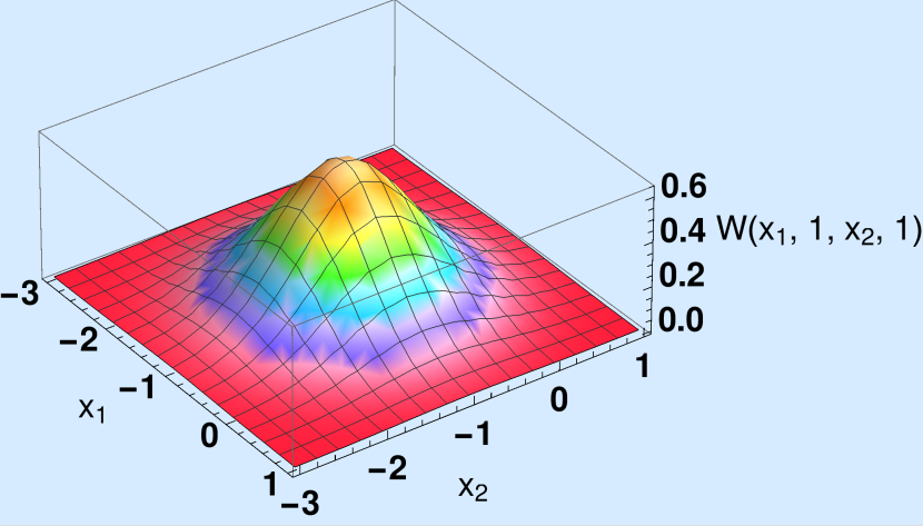
projection on $(p_{1},p_{2})=(1,1)$ plane.

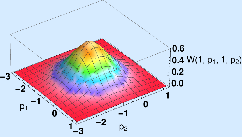
projection on $(x_{1},x_{2})=(1,1)$ plane.

Figure 1: Wigner distribution $W(1,1,x_{2},p_{2})$, $W(x_{1},p_{1},1,1)$, $W(x_{1},1,x_{2},1)$ and $W(1,p_{1},1,p_{2})$ shows no entanglement effect.

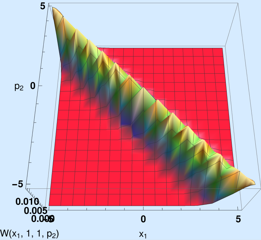
Projection on $(p_{1},x_{2})=(1,1)$ plane

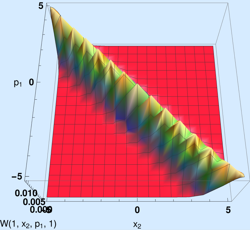
Projection on $(x_{1},p_{2})=(1,1)$ plane

Figure 2: Wigner distribution $W(x_{1},1,1,p_{2})$ and $W(1,x_{2},p_{1},1)$ are exhibiting the entanglement effects. They are not appearing as a separated Gaussian distribution.

For the illustration purpose, let us choose

$$\langle\hat{x}_{1}^{2}\rangle=\langle\hat{x}_{2}^{2}\rangle=\langle\hat{p}_{1}^{2}\rangle=\langle\hat{p}_{2}^{2}\rangle=\frac{1}{2},$$

$$\langle\hat{x}_{1}\hat{p}_{2}\rangle=\langle\hat{p}_{1}\hat{x}_{2}\rangle=-\frac{1}{2}.$$ (98)

Since our $W$ is on four-dimensional phase space, we have to project it onto two-dimensional space to visualize it graphically. The FIG. 1 represents the projection of WQD onto $(x_{1},p_{1})=(1,1)$, $(x_{2},p_{2})=(1,1)$, $(p_{1},p_{2})=(1,1)$ and $(x_{1},x_{2})=(1,1)$ planes respectively. They exhibit no entanglement effect. Being projected onto the two-dimensional phase-space, they appear to be an individual Gaussian distribution. However, from FIG. 2, one can envisage the entanglement of the co-ordinates $(x_{1},p_{2})$ and $(x_{2},p_{1})$. In particular, $x_{1}$ is entangled with $p_{2}$ and $x_{2}$ is entangled with $p_{1}$. This confirms the indications we had to get from the correlations in the previous section. In particular, the figures are consistent with the correlations matrix (variance matrix) of the last section.

VI Experimental connections

VI.1 Szilard engine cycle

One of the possibilities of results of the present study is to use it for the Szilard engine cycle szilard ; szilard1 ; szilard2 ; szilard3 ; szilard4 ; szilard5 for a bipartite system. Gaussian measurement performed by the second party (corresponding to $x_{2}$) corresponds to the variance matrix measurementgaussian

$$\hat{\gamma}^{\pi_{2}}=\hat{R}(\theta_{\pi_{2}})\mbox{diag}(\mu/2,\mu^{-1}/2)\hat{R}^{T}(\theta_{\pi_{2}}),\;\;\mu\in[0,\infty).$$ (99)

Where the rotation operator is given through the Pauli matrix by $\hat{R}(\theta_{\pi_{2}})=\cos\theta_{\pi_{2}}\hat{\mathbb{I}}-i\sin\theta_{\pi_{2}}\hat{\sigma}_{y}$. The measurement parameter $\mu=0$ and $\mu=1$ corresponds to homodyne and heterodyne measurement respectively. The conditional state covariance matrix is given by

$$\hat{V}_{11}^{\pi_{2}}=\hat{V}_{11}-\hat{V}_{12}(\hat{V}_{22}+\hat{\gamma}^{\pi_{2}})^{-1}\hat{V}_{12}^{T}.$$ (100)

Then the extractable work ($W_{se}=K_{B}T[S(V_{11})-S(V_{11}^{\pi_{2}})]$) due to the measurement backreaction is given by

$$W_{se}=\frac{1}{2}k_{B}T\ln\left(\frac{det(\hat{V}_{11})}{det(\hat{V}_{11}^{\pi_{2}})}\right),$$ (101)

where we have used the Rényi entropy of order $2$, $S_{2}(\rho)=-\ln(Tr(\rho^{2}))$, which in case of Gaussian state becomes $S_{2}(V_{12})=\frac{1}{2}\ln(det(V_{12}))$.
In the concerned case of this present paper, for a heterodyne measurement ($\mu=1$), the extractable work is reduecd to

$$W_{se}=-\frac{1}{2}k_{B}T\ln\left[\left(1+\frac{\Lambda_{12}^{2}}{(d+2\Lambda_{11})}\right)\left(1+\frac{\Lambda_{12}^{2}}{d(1+2\Lambda_{22})}\right)\right]\neq 0.$$ (102)

In particular, the non-commutativity of the space opens up a possibility of extractable work protocol.

VI.2 Determination of the signature of noncommutative of space: an Opto-mechanical scheme

The optomechanical scheme is realized through an interaction between an optical pulse and a mechanical oscillator expt1 ; expt2 . The setup consists of a half-silvered mirror, two Fabry-Perot cavities, a laser source, and a detector (for instance see expt1 ; expt2 ; expt3 ), on which a sequence of four radiation pressure interactions form an optical cavity (resonator) yielding the interaction operator

$$\hat{\zeta}_{lm}=\hat{U}_{lm,p}\hat{U}_{lm,x}^{\dagger}\hat{U}_{lm,p}^{\dagger}\hat{U}_{lm,x},\;\mbox{with}\;\hat{U}_{lm,p}=e^{i\hat{n}_{l}\sum_{j=1}^{2}\lambda_{jl}\hat{\tilde{P}}_{j}^{m}},\;\hat{U}_{lm,x}=e^{i\hat{n}_{l}\sum_{j=1}^{2}\lambda_{jl}\hat{\tilde{X}}_{j}^{m}},$$ (103)

where the index $m$ and $l$ stand for the identification of the mechanical quantities and the optical degrees of freedom, respectively, and $\lambda_{l}=(\lambda_{1l},\lambda_{2l})$ is the optical field interaction length. $\hat{\zeta}_{lm}$ displaces the mechanical state around complete loop in phase space, thus creating an additional phase, which is measurable in a tabletop experiment, in principle. In particular, the mean of the optical field operator

$$\langle\hat{a}\rangle=\langle\alpha|\hat{\zeta}_{lm}^{\dagger}\hat{a}\hat{\zeta}_{lm}|\alpha\rangle=\langle\hat{a}\rangle_{QM}e^{-i\Theta}$$ (104)

provides the additional phase ($\Theta$) on the light arising due to the presence of the noncommutative oscillator. Whereas, the mean of the annihilation operator $\hat{a}$ of the optical field $|\alpha\rangle$ (the input optical coherent state with mean photon number $n_{p}$) using the standard quantum mechanics (with commutative space) reads

$$\langle\hat{a}\rangle_{QM}=\alpha e^{-i|\lambda_{l}|^{2}-n_{p}(1-e^{-2i|\lambda_{l}|^{2}})}.$$ (105)

The additional phase factor $\Theta$ depends on the product of the noncommutative parameters ($\theta\eta$). That means the nonzero $\Theta$ implies both position-position and momentum-momentum noncommutativity.

VII Conclusions

In this paper, we have studied in detail the entanglement property of two dimensional anisotropic (a fairly general form of anisotropy) harmonic oscillator (AHO, where the entanglement is induced by both the spatial and momentum non-commutativity. It turns out that the bipartite Gaussian state (BGS) is almost always entangled. Simon’s separability criterion shows that BGS is separable for a set of specific values of the masses and frequencies of the oscillators. The explicit form of the constraint equation is determined in the present paper. An additional interaction term, dependent upon the noncommutativity parameter $\theta$ and $\eta$, is generated by Bopp’s shift, which is the main source for the entanglement between the coordinates and momentum degrees of freedom.
Wigner quasiprobability distribution (WQD) for the ground state of our system is computed. Projecting the four-dimensional phase space WQD onto two dimensions, we have graphically identified the exact degrees of freedom, which are entangled. This is also demonstrated by calculating the correlations (variances) between the observables. This opens up the possibility of direct experimental observation through interferometry. In particular, the obtained coherent state structure can be utilized in an optomechanical setup that helps us to transfer the information of a noncommutative anisotropic oscillator to the high-intensity optical pulse in terms of a sequence of opto-mechanical interaction inside an optical resonator expt1 ; expt2 ; expt3 ; expt4 ; expt5 . Consequently, the optical phase shift is easily measurable with very high accuracy through an interferometric system as stated in expt1 . This makes the whole procedure much easier to collect the pieces of information of noncommutative structures through optical systems already available to us. In particular, by comparing the phase difference of the input signal and output signal after interaction of the input signal with the mechanical anisotropic oscillator inside the cavity, and comparing the phase difference with the prediction of usual quantum mechanics, we can determine the signature of quantum gravity (if any). Thus, it may bypass all the difficulties of probing high energy scales through scattering experiments. However, we would like to mention that, within this type of experimental set-up only the product $\theta\eta$ are determined, not the individual $\theta$ and $\eta$. Moreover, the typical size ( distance between mirrors) of the resonant cavity for a Fabry-Perot Interferometer should be an order of a few kilometers to have any detectable effect in this scenario expt1 .
Moreover, the amount of extractable work for a heterodyne measurement through Szilard engine cycle for our bipartite system is outlined in this paper. This shows the applicability of our results in thermodyanmic process, i.e, in engineering applications.
In terms of constructor-theoretic principles marletto1 ; bose1 , if we observe the entanglement effects in the measurement of the properties of two quantum masses that interact with each other through gravity only, then we can conclude that the mediator (gravity) got to have some quantum features marletto1 ; bose1 . It doesn’t matter in what way gravity is quantum - whether it’s loop quantum gravity or string theory or something else - but it has to be a quantum theory. We have seen in the present paper that the entanglement in co-ordinate degrees of freedom is solely depends on the noncommutative parameters. Thus any experimental signature of entanglement for the present scenario will indicate the signature of noncommutativity of space.

VIII Acknowledgement

I am grateful to the anonymous referees for their valuable suggestions.
This research was supported in part by the International Centre for Theoretical Sciences (ICTS) for the online program - Non-Hermitian Physics (code: $ICTS/nhp2021/3$).

IX Conflict of interest

The author declares that there is no conflict of interest for the present article.

X Data availability statement

Data sharing is not applicable to this article as no new data were created or analyzed in this study.

Appendix A Diagonalization of $\hat{\Omega}$

$\hat{\Omega}$ is a normal matrix. So, $\hat{\Omega}$ is diagonalizable through a similarity transformation

$$\hat{\Omega}_{D}=\hat{Q}^{-1}\hat{\Omega}\hat{Q}.$$ (106)

$\hat{Q}^{-1}$ and $\hat{Q}$ are obtained by arranging the left and right eigenvectors column-wise, respectively. Since, $\hat{\Omega}$ is not a symmetric matrix ($\hat{\Omega}^{T}\neq\hat{\Omega}$), the left and right eigenvectors of $\hat{\Omega}$ are not same. However, the left and right eigenvalues are the same. The characteristic polynomial ($p(\lambda)=\det(\lambda\mathbb{\hat{I}}-\hat{\Omega}),$) of $\hat{\Omega}$ is given by

$$p(\lambda)=\lambda^{4}+b\lambda^{2}+c.$$ (107)

Where

$$c = \omega_{x}^{2}\omega_{y}^{2},$$ (108)

$$b = \alpha_{0}\omega_{x}^{2}+\frac{1}{\alpha_{0}}\omega_{y}^{2}+4\nu_{1}\nu_{2}(\sqrt{\alpha_{0}}+\frac{1}{\sqrt{\alpha_{0}}})^{2}.$$ (109)

With

$$\omega_{x}^{2} = 4\nu_{1}\nu_{2}(\frac{\mu_{1}\omega_{1}^{2}}{4\mu_{2}\nu_{2}^{2}}-1),$$ (110)

$$\omega_{y}^{2} = 4\nu_{1}\nu_{2}(\frac{\mu_{2}\omega_{2}^{2}}{4\mu_{1}\nu_{1}^{2}}-1),$$ (111)

$$\alpha_{0} = \frac{\mu_{2}\nu_{2}}{\mu_{1}\nu_{1}}.$$ (112)

using the explicit forms of $\mu_{i},\nu_{i},\omega_{i},\;i=1,2$, one can show that $c\geq 0,\;b\geq 0$ as follows.

A.1 Proof of $b\geq 0$, $c\geq 0$

We have

$$b = \omega_{1}^{2}+\omega_{2}^{2}+6\nu_{1}\nu_{2},$$ (113)

$$c = \omega_{1}^{2}\omega_{2}^{2}+16\nu_{1}^{2}\nu_{2}^{2}-4\nu_{1}^{2}\omega_{1}^{2}\mu_{1}/\mu_{2}-4\nu_{2}^{2}\omega_{2}^{2}\mu_{2}/\mu_{1}.$$ (114)

Clearly, $b>0$ for nonzero positive values of $\omega_{1},\omega_{2},\nu_{1},\nu_{2}$.
First we observe that, $c$ can be factorized as

$$c=16\nu_{1}^{2}\nu_{2}^{2}\left(\frac{\mu_{1}\omega_{1}^{2}}{4\mu_{2}\nu_{2}^{2}}-1\right)\left(\frac{\mu_{2}\omega_{2}^{2}}{4\mu_{1}\nu_{1}^{2}}-1\right).$$ (115)

If we use the explicit forms of $\omega_{1},\omega_{2},\nu_{1},\nu_{2}$, we have

$$\frac{\mu_{1}\omega_{1}^{2}}{4\mu_{2}\nu_{2}^{2}} = \frac{4m_{2}^{2}\hbar^{2}}{(\eta+m_{1}m_{2}\theta\tilde{\omega}_{1}^{2})^{2}}\left(m_{1}\tilde{\omega}_{1}^{2}+\frac{\eta^{2}}{4\hbar^{2}m_{2}}\right)\left(\frac{1}{m_{2}}+\frac{1}{4\hbar^{2}}m_{1}\tilde{\omega}_{1}^{2}\theta^{2}\right)$$ (116)

$$= \left(1+\frac{4\hbar^{2}}{\eta^{2}}m_{1}m_{2}\tilde{\omega}_{1}^{2}\right)\left(1+\frac{\theta^{2}}{4\hbar^{2}}m_{1}m_{2}\tilde{\omega}_{1}^{2}\right)\left(1+\frac{\theta}{\eta}m_{1}m_{2}\tilde{\omega}_{1}^{2}\right)^{-2}$$

$$= \frac{1}{\left(1+\frac{\theta}{\eta}m_{1}m_{2}\tilde{\omega}_{1}^{2}\right)^{2}}\left(\left(1+\frac{\theta}{\eta}m_{1}m_{2}\tilde{\omega}_{1}^{2}\right)^{2}+\frac{2\theta}{\eta}m_{1}m_{2}\tilde{\omega}_{1}^{2}(\frac{2\hbar^{2}}{\eta\theta}+\frac{\eta\theta}{8\hbar^{2}}-1)\right)$$

$$= 1+\frac{2\theta m_{1}m_{2}\tilde{\omega}_{1}^{2}}{\eta\left(1+\frac{\theta}{\eta}m_{1}m_{2}\tilde{\omega}_{1}^{2}\right)^{2}}\left(\frac{\sqrt{2}\hbar}{\sqrt{\eta\theta}}-\frac{\sqrt{\eta\theta}}{2\sqrt{2}\hbar}\right)^{2}\geq 1.$$

Similarly, we see that

$$\frac{\mu_{2}\omega_{2}^{2}}{4\mu_{1}\nu_{1}^{2}}=1+\frac{2\theta m_{1}m_{2}\tilde{\omega}_{2}^{2}}{\eta\left(1+\frac{\theta}{\eta}m_{1}m_{2}\tilde{\omega}_{2}^{2}\right)^{2}}\left(\frac{\sqrt{2}\hbar}{\sqrt{\eta\theta}}-\frac{\sqrt{\eta\theta}}{2\sqrt{2}\hbar}\right)^{2}\geq 1.$$ (117)

Therefore, we have

$$c\geq 0.$$ (118)

Moreover, the discriminant of the characteristic polynomial

$$\Delta = b^{2}-4c$$ (119)

$$= \left(\alpha_{0}\omega_{x}^{2}-\frac{1}{\alpha_{0}}\omega_{y}^{2}\right)^{2}+8\nu_{1}\nu_{2}(1+\alpha_{0})^{2}(\omega_{x}^{2}+\omega_{y}^{2})+\frac{4\nu_{1}^{2}\nu_{2}^{2}}{\alpha_{0}^{2}}(1+\alpha_{0})^{4}$$

is positive definite. It can be easily verified that

$$\lambda^{2}=\frac{1}{2}(-b\pm\sqrt{\Delta})\leq 0.$$ (120)

A.2 Eigenvalues and eigenvectors of $\hat{\Omega}$

From  (120), we can see that $\hat{\Omega}$ has four distinct imaginary eigen-values

$$\lambda=\left\{-i\lambda_{1},i\lambda_{1},-i\lambda_{2},i\lambda_{2}\right\}.$$ (121)

Where

$$\lambda_{1}=\frac{1}{\sqrt{2}}\sqrt{b+\sqrt{\Delta}},\;\lambda_{2}=\frac{1}{\sqrt{2}}\sqrt{b-\sqrt{\Delta}}.$$ (122)

Let us consider the eigenvalue equations of $\hat{\Omega}$ as follows.

$$u_{j}\hat{\Omega} = -i\lambda_{j}u_{j},\;j=1,2.$$ (123)

$$u_{j}^{*}\hat{\Omega} = i\lambda_{j}u_{j}^{*}\;,j=1,2.$$ (124)

$$\hat{\Omega}v_{j} = -i\lambda_{j}v_{j},\;j=1,2.$$ (125)

$$\hat{\Omega}v_{j}^{*} = i\lambda_{j}v_{j}^{*},\;j=1,2.$$ (126)

Then the following identities hold quite generally.

$$u_{i}^{*}v_{j}=u_{i}v_{j}^{*},\;u_{i}v_{j}=u_{i}^{*}v_{j}^{*}=\delta_{ij},\;\forall i,j=1,2.$$ (127)

(127) suggests the following conditions between the left and right eigen-vectors.

$$v_{i}=-\Sigma_{y}u_{i}^{\dagger},\;(i=1,2).$$ (128)

In our case, the explicit form of the left eigenvectors $u_{i},\;(i=1,2)$ are given by

$$u_{i}=\frac{1}{k_{i}}\left(\begin{array}[]{c}-i\lambda_{i}\mu_{1}\mu_{2}(\lambda_{i}^{2}-\omega_{2}^{2}-4\nu_{1}\nu_{2})\\ \mu_{2}(\lambda_{i}^{2}-\omega_{2}^{2})+4\mu_{1}\nu_{1}^{2}\\ 2\nu_{1}\mu_{1}\mu_{2}(\lambda_{i}^{2}-4\nu_{1}\nu_{2})+2\nu_{2}\mu_{2}^{2}\omega_{2}^{2}\\ 2i\lambda_{i}(\mu_{1}\nu_{1}+\mu_{2}\nu_{2})\end{array}\right)^{T}.$$ (133)

The right eigenvectors can be constructed from  (128) in a straighforward manner.

A.3 Similarity transformation

Now the similarity transformation $\hat{Q}$ (as well as $\hat{Q}^{-1}$) can be constructed by arranging the eigen-vectors columnwise. In particular,

$$\hat{Q} = (v_{1},v_{1}^{*},v_{2},v_{2}^{*}),$$ (134)

$$\hat{Q}^{-1} = (u_{1}^{T},(u_{1}^{*})^{T},u_{2}^{T},(u_{2}^{*})^{T}).$$ (135)

One can verify that

$$\hat{Q}^{\dagger}=-\hat{\Sigma}_{z}\hat{Q}^{-1}\hat{\Sigma}_{y},$$ (136)

with

$$\hat{\Sigma}_{z}=\mbox{diag}(\sigma_{z},\sigma_{z}).$$ (137)

Now, using  (106), we have the diagonalization representation $\hat{\Omega}_{D}$ of $\hat{\Omega}$ as

$$\hat{\Omega}_{D}=\mbox{diag}(-i\lambda_{1},i\lambda_{1},-i\lambda_{2},i\lambda_{2}).$$ (138)

The similarity transformation suggests a new co-ordinate vector $\hat{\zeta}$, which is connected with the original co-ordinate vector $X$ of  (29) through

$$\hat{\zeta}=\hat{Q}^{-1}X.$$ (139)

Then, using  (136), we can write

$$X^{\dagger} = \hat{\zeta}^{\dagger}(-\hat{\Sigma}_{z}\hat{Q}^{-1}\hat{\Sigma}_{y}).$$ (140)

A.4 Equivalent dynamics in diagonal representation

The time-dependent Schrödinger equation

$$\hat{H}\psi=i\hbar\frac{\partial\psi}{\partial t},$$ (141)

is transformed with the similarity transformation as follows.

$$\hat{Q}^{-1}\frac{1}{2}X^{\dagger}\hat{\mathcal{H}}X\psi\hat{Q} = i\hbar\hat{Q}^{-1}\frac{\partial\psi}{\partial t}\hat{Q}.$$ (142)

$$\therefore\frac{1}{2}\hat{\zeta}^{\dagger}\Sigma\hat{\zeta}\tilde{\psi}_{Q} = i\hbar\frac{\partial\tilde{\psi}_{Q}}{\partial t}.$$ (143)

Where

$$\hat{\Sigma}=\mbox{diag}(\lambda_{1},\lambda_{1},\lambda_{2},\lambda_{2}),$$ (144)

$$\tilde{\psi}_{Q}=\hat{Q}^{-1}\psi\hat{Q}.$$ (145)

That means, the new diagonal Hamiltonian

$$\hat{H}_{D}=\frac{1}{2}\zeta^{\dagger}\hat{\Sigma}\zeta$$ (146)

obeys the same dynamics as that of $\hat{H}$, with the new co-ordinate vector $\zeta$.
If we compute the commutators of the components of $\hat{\zeta}$, then we can identify that they forms a set of independent annihilation and creation operators. In particular,

$$\left[\hat{\zeta}_{k},\hat{\zeta}_{l}^{\dagger}\right]=\delta_{kl};\;k,l=1,2.$$ (147)

Where

$$\hat{\zeta}=(\hat{\zeta}_{1},\hat{\zeta}_{1}^{\dagger},\hat{\zeta}_{2},\hat{\zeta}_{2}^{\dagger})^{T}.$$ (148)

References

- (1) A. Ashtekar and R. Geroch, “Quantum theory of gravitation”, Rep. Prog. Phys. 37 1211 (1974).
- (2) K.S. Stelle, “The unification of quantum gravity”, Nuclear Physics B - Proceedings Supplements 88 3-9 (2000).
- (3) https://home.cern/science/engineering/restarting-lhc-why-13-tev. Last visited .
- (4) C. Pfeifer and J. J. Relancio, “Deformed relativistic kinematics on curved spacetime: a geometric approach”, Eur. Phys. J. C 82 150 (2022).
- (5) S. Liberati, “Tests of Lorentz invariance: a 2013 update”, Class. Quantum Gravity 30 133001 (2013).
- (6) N. Seiberg and E. Witten, “String theory and noncommutative geometry”, Journal of High Energy Physics 09 (1999).
- (7) J. M. Romero, J. D. Vergara, and J. A. Santiago, “Noncommutative spaces, the quantum of time, and Lorentz symmetry”, Phys. Rev. D 75 065008 (2007).
- (8) L. Lawson, L. Gouba and G. Y. Avossevou, “Two-dimensional noncommutative gravitational quantum well”, J. Phys. A: Math. Theor. 50 475202 (2017).
- (9) F. Vega, “Oscillators in a ()-dimensional noncommutative space ”, J. Math. Phys. 55 032105 (2014).
- (10) R. Banerjee, B. Chakraborty, S. Ghosh, P. Mukherjee and S. Samanta, “Topics in Noncommutative Geometry Inspired Physics”, Found Phys 39 1297 (2009).
- (11) S. Ghosh, S. Gangopadhyay and P. K. Panigrahi, “Noncommutative quantum cosmology with perfect fluid”, Modern Physics Letters A 37 2250009 (2022).
- (12) R. J. Szabo, “Quantum field theory on noncommutative spaces”, Physics Reports 378 207-299 (2003).
- (13) M. R. Douglas and N. A. Nekrasov, “Noncommutative field theory ”, Rev. Mod. Phys. 73 977 (2001).
- (14) M. Pitkin, S. Reid, S. Rowan and J. Hough, “Gravitational Wave Detection by Interferometry (Ground and Space)”, Living Rev. Relativ. 14 5 (2011).
- (15) C. L. Ching, W. K. Ng, “Deformed Gazeau-Klauder Schrödinger cat states with modified commutation relations”, Phys. Rev. D 100 085018 (2019).
- (16) J. F. G. Santos, “Noncommutative phase-space effects in thermal diffusion of Gaussian states”, J. Phys. A: Math. Theor. 52 405306 (2019).
- (17) P. Chattopadhyay, A. Mitra and G. Paul, “Uncertainty Relations in Non-Commutative Space”, Int. J. Theor. Phys. 58 2619-2631 (2019).
- (18) U. D. Jentschura, “Gravitational effects in -factor measurements and high-precision spectroscopy: Limits of Einstein’s equivalence principle”, Phys. Rev. A 98 032508 (2018).
- (19) D. Buono, G. Nocerino, V. D’Auria, A. Porzio, S. Olivares, and M. G. A. Paris, “Quantum characterization of bipartite Gaussian states ”, Journal of the Optical Society of America B 27 A110-A118 (2010).
- (20) S. Ma, M. J. Woolley, X. Jia and J. Zhang, “Preparation of bipartite bound entangled Gaussian states in quantum optics“, Phys. Rev. A 100, 022309 (2019).
- (21) S. M. Vermeulen et al, “An experiment for observing quantum gravity phenomena using twin table-top 3D interferometers ”Class. Quantum Grav. 38 085008 (2021).
- (22) J. A. de F. Pacheco, S. Carneiro and J. C. Fabris, “Gravitational waves from binary axionic black holes”, Eur. Phys. J. C 79 426 (2019).
- (23) M. J. Koop and L. S. Finn, “Physical response of light-time gravitational wave detectors”, Phys. Rev. D 90 062002 (2014).
- (24) A. Muhuri, D. Sinha and S. Ghosh, “Entanglement induced by noncommutativity: anisotropic harmonic oscillator in noncommutative space”, Eur. Phys. J. Plus 136 35 (2021).
- (25) M. C. Eser and M. Riza, “Energy corrections due to the noncommutative phase-space of the charged isotropic harmonic oscillator in a uniform magnetic field in 3D”, Phys. Scr. 96 085201 (2021).
- (26) B. Lin, J. Xu, T. Heng, “Induced entanglement entropy of harmonic oscillators in non-commutative phase space ”, Modern Physics Letters A 34 1950268 (2019).
- (27) C. Bastos, A. E. Bernardini, O. Bertolami, N. C. Dias and J. N. Prata, “Entanglement due to noncommutativity in phase space”, Phys. Rev. D 88 085013 (2013).
- (28) R. Simon, “Peres-Horodecki Separability Criterion for Continuous Variable Systems ”, Phys. Rev. Lett. 84 2726 (2000).
- (29) A. Peres, “Separability Criterion for Density Matrices”, Phys. Rev. Lett. 77 1413 (1996).
- (30) P. Horodecki, “Separability criterion and inseparable mixed states with positive partial transposition”, Physics Letters A 232 333-339 (1997).
- (31) S. Biswas, P. Nandi and B. Chakraborty, “Emergence of a geometric phase shift in planar noncommutative quantum mechanics”, Phys. Rev. A 102 022231 (2020).
- (32) L. Gouba, “A comparative review of four formulations of noncommutative quantum mechanics”, International Journal of Modern Physics A 31 1630025 (2016).
- (33) O. Bertolami, J. G. Rosa, C. M. L. De Aragão, P. Castorina, D. Zappalà, “Scaling of variables and the relation between noncommutative parameters in Noncommutative Quantum Mechanics”, Modern Physics Letters A 21 795-802 (2006).
- (34) O. Bertolami, J. G. Rosa, C. M. L. De Aragão, P. Castorina, D. Zappalà, “Noncommutative gravitational quantum well”, Phys. Rev. D 72 025010 (2005).
- (35) Arvind, N. Mukunda, R. Simon “The real symplectic groups in quantum mechanics and optics ”, Pramana - J Phys 45 471-497 (1995).
- (36) J. Eisert, T. Tyc, T. Rudolph, B. C. Sanders, “Gaussian Quantum Marginal Problem”, Commun. Math. Phys. 280 263-280 (2008).
- (37) V. V. Dodonov, “Invariant Quantum States of Quadratic Hamiltonians ”, Entropy 2031 634 (2021).
- (38) M. Moshinsky and P. Winternitz, “Quadratic Hamiltonians in phase space and their eigenstates ”, J. Math. Phys. 21 1667 (1980).
- (39) L. Qiong-Gui, “Anisotropic Harmonic Oscillator in a Static Electromagnetic Field”, Commun. Theor. Phys. 38 667 (2002).
- (40) G. Esposito, G. Marmo and G. Sudarshan, “From Classical to Quantum Mechanics: An Introduction to the Formalism, Foundations and Applications. ”, Cambridge: Cambridge University Press, ISBN:9780511610929 (2010).
- (41) B. G. da Costa, G. A. C. da Silva, I. S. Gomez, “Supersymmetric quantum mechanics and coherent states for a deformed oscillator with position-dependent effective mass”, J. Math. Phys. 62 092101 (2021).
- (42) C. Fabre and N. Treps, “Modes and states in quantum optics”, Rev. Mod. Phys. 92 035005 (2020).
- (43) R. Simon, E. C. G. Sudarshan, N. Mukunda, ‘Gaussian-Wigner distributions in quantum mechanics and optics’, Phys. Rev. A 36 3868 (1987).
- (44) D. K. Ferry, ‘Phase-space functions: can they give a different view of quantum mechanics? ’, J Comput Electron 14 864 (2015).
- (45) U. Ravaioli, M. A. Osman, W. Pötz, N. Kluksdahl, D. K. Ferry, ‘Investigation of ballistic transport through resonant-tunneling quantum wells using Wigner function approach.’, Physica B 134 36 (1985).
- (46) G. V. Dunne, “Topological aspects of low dimensional systems”, vol 69. Springer, Berlin, Heidelberg., Online ISBN978-3-540-46637-6 (1999)
- (47) G. Cariolaro, G. Pierobon, “Fock expansion of multimode pure Gaussian states”, J. Math. Phys. 56 122109 (2015).
- (48) X. Ma, William Rhodes, “Multimode squeeze operators and squeezed states”, Phys. Rev. A 41, 4625 (1990).
- (49) A. Ferraro, S. Olivares, Matteo G. A. Paris, “Gaussian States in Quantum Information”, Napoli Series on physics and Astrophysics. Bibliopolis, ISBN 88-7088-483-X (2005).
- (50) L. Szilard, “Über die Entropieverminderung in einem thermodynamischen System bei Eingriffen intelligenter Wesen”, Zeitschrift für Physik 53 840-856 (1929).
- (51) X. L. Huang, A. N. Yang, H. W. Zhang, S. Q. Zhao, S. L. Wu, “Two particles in measurement-based quantum heat engine without feedback control”, Quantum Inf Process 19 242 (2020).
- (52) A. Tuncer, M. Izadyari, C. B. Dağ, F. Ozaydin, Ö. E. Müstecaplıoğlu, “Work and heat value of bound entanglement”, Quantum Inf Process 18 373 (2019).
- (53) M. Cuzminschi, A Zubarev, A. Isar, “Extractable quantum work from a two-mode Gaussian state in a noisy channel”, Sci Rep 11 24286 (2021).
- (54) H. T, Quan, Y. X. Liu, C. P. Sun, F. Nori, “Quantum thermodynamic cycles and quantum heat engines”, Phys. Rev. E 76 031105 (2007).
- (55) A. de Oliveira Junior, M. C. de Oliveira, “Unravelling the non-classicality role in Gaussian heat engines”, Sci Rep 12 10412 (2022).
- (56) M. Brunelli, M. G. Genoni, M. Barbieri, M. Paternostro, “Detecting Gaussian entanglement via extractable work”, Phys. Rev. A 96 062311 (2017).
- (57) S. Dey, A. Bhat, D. Momeni, M. Faizal, A. F. Ali, T. K. Dey, A. Rehman, “Probing noncommutative theories with quantum optical experiments”, Nuclear Physics B 924 578-587 (2017).
- (58) I. Pikovski, M. R. Vanner, M. Aspelmeyer, M. S. Kim, Ĉ. Brukner, “Probing Planck-scale physics with quantum optics”, Nature Phys 8 393-397 (2012).
- (59) P. Bosso, S. Das, I. Pikovski, M. R. Vanner, “Amplified transduction of Planck-scale effects using quantum optics”, Phys. Rev. A 96 023849 (2017).
- (60) C. K. Law, “Interaction between a moving mirror and radiation pressure: A Hamiltonian formulation”, Phys. Rev. A 51 2537 (1995).
- (61) M. R. Vanner, J. Hofer, G. D. Cole, M. Aspelmeyer, “Cooling-by-measurement and mechanical state tomography via pulsed optomechanics”, Nat Commun 4 2295 (2013).
- (62) C. Marletto, V. Vedral, “Gravitationally Induced Entanglement between Two Massive Particles is Sufficient Evidence of Quantum Effects in Gravity”, Phys. Rev. Lett. 119 240402 (2017).
- (63) S. Bose et al., “Spin Entanglement Witness for Quantum Gravity”, Phys. Rev. Lett. 119 240401 (2017).