Tight bounds for the learning of homotopy à la Niyogi, Smale, and Weinberger for subsets of Euclidean spaces and of Riemannian manifolds

Abstract

In this article we extend and strengthen the seminal work by Niyogi, Smale, and Weinberger on the learning of the homotopy type from a sample of an underlying space. In their work, Niyogi, Smale, and Weinberger studied samples of $C^{2}$ manifolds with positive reach embedded in $\mathbb{R}^{d}$. We extend their results in the following ways: In the first part of our paper we consider both manifolds of positive reach — a more general setting than $C^{2}$ manifolds — and sets of positive reach embedded in $\mathbb{R}^{d}$. The sample $P$ of such a set ${\mathcal{S}}$ does not have to lie directly on it. Instead, we assume that the two one-sided Hausdorff distances — $\varepsilon$ and $\delta$ — between $P$ and ${\mathcal{S}}$ are bounded. We provide explicit bounds in terms of $\varepsilon$ and $\delta$, that guarantee that there exists a parameter $r$ such that the union of balls of radius $r$ centred at the sample $P$ deformation-retracts to ${\mathcal{S}}$. To be more concrete:

• We provide tight bounds on $\varepsilon$ and $\delta$ for sets of positive reach. We exhibit their tightness by an explicit construction.

• We also provide tight bounds in the case where the set ${\mathcal{S}}$ is a manifold, thus improving the bounds given by Niyogi, Smale, and Weinberger. Again, we prove the tightness of the bounds by constructing explicit examples.

• We simplify Niyogi, Smale, and Weinberger’s proof using Federer’s work on the reach, and several geometric observations. It is thanks to the streamlined proof that we can easily extend the reconstruction from $C^{2}$ manifolds to sets of positive reach. We also carefully distinguish the roles of $\delta$ and $\varepsilon$, which is essential to achieve tight bounds. The separation of $\delta$ and $\varepsilon$ is sensible in practical situations, where the noise is generally much smaller than the sample density.

In the second part of our paper we study homotopy learning in a significantly more general setting — we investigate sets of positive reach and submanifolds of positive reach embedded in a Riemannian manifold with bounded sectional curvature. To this end we introduce a new version of the reach in the Riemannian setting inspired by the cut locus. Yet again, we provide tight bounds on $\varepsilon$ and $\delta$ for both cases (submanifolds as well as sets of positive reach), exhibiting the tightness by an explicit construction.

1 Introduction

Can we infer the topology of a set if we are only given partial geometric information about it? Under which conditions is such inference possible?

These questions were first motivated by the shape reconstruction of objects in 3-dimensional Euclidean space. There, the partial geometric information was represented by a finite, in general noisy, set of points obtained from photogrammetric or lidar measurements [10, 17, 19, 20, 30].

More recently, the same questions have arisen in the context of learning and topological data analysis (TDA). In these fields, one seeks to recover a (relatively) low-dimensional support of a probability measure in a high-dimensional space, given a (finite) data set drawn from this probability measure [21, 27, 39, 35]. Assuming the support is a manifold, one calls this process manifold learning [63].

In [61], Niyogi, Smale, and Weinberger showed that, given a $C^{2}$ manifold of positive reach embedded in Euclidean space and a sufficiently dense point sample on (or near) the manifold, the union of balls of certain radii centred on the point sample captures the homotopy type of the manifold. By the nerve theorem, the homotopy type of the union of balls is shared by the Čech complex [18, 40] and $\alpha$-complex [38] of the point sample. From these complexes we can then learn the topological information such as the homology groups of the underlying manifold. Niyogi, Smale, and Weinberger’s homotopy learning result has led to numerous generalizations including [11, 13, 25, 52, 72].

We revisit the work of Niyogi, Smale, and Weinberger, generalizing the settings of their work in various ways and providing tight bounds on the sample quality in each of the generalizations. In the first part of our paper, we drop the condition of being $C^{2}$ and study manifolds of positive reach embedded in Euclidean space and, more generally, sets of positive reach in Euclidean space, such as the one depicted in Figure 1.

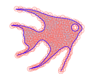
Figure 1: Left: A fish shaped set ${\mathcal{S}}$ of positive reach (in blue). Its medial axis (in purple) is at a positive distance. For $0\leq i\leq 3$, we also represent the normal cone of $p_{i}$ with respect to ${\mathcal{S}}$ (after an intersection with a small disk and a translation to $p_{i}$). The normal cone of the point $p_{2}$ is $p_{2}$ itself. Right: The set ${\mathcal{S}}$ with a sample $P$ and a thickening of $P$. We see that the thickening has the same homotopy type as ${\mathcal{S}}$.

In the second part of the paper we infer the homotopy of subsets and submanifolds of positive reach of Riemannian manifolds with bounded (sectional) curvatures. It requires some thought to generalize the notion of ‘the reach’ to these settings. We formulate the appropriate definition and provide tight bounds on the sample quality also in this case.

2 State-of-the-art

2.1 Sets of positive reach

Our extension of Niyogi, Smale, and Weinberger’s result to sets of positive reach — as well as improvement of their results on manifolds — relies on the work of Federer [41], which Niyogi, Smale, and Weinberger seem to have been unaware of. In particular, we use Federer’s generalization of normal spaces to normal cones (see Figure 1 (left)for a pictorial introduction and Appendix A.1 for a full definition) and his different characterizations of the normal cone as a key building block. We recall the relevant results from Federer’s work in Appendix A.1.

We note that the reach can be estimated from a sample [2, 3, 15].

Subsets of positive reach of Riemannian manifolds were studied extensively by Kleinjohann [53, 54] and Bangert [14] in generalization of Federer’s theory [41] for subsets of Euclidean space. Boissonnat and Wintraecken investigated yet another definition of the reach for subsets of Riemannian manifolds in [22].

2.2 Homotopy learning

For some particular cases, the best previously known bounds on the distance between a manifold (or a set) of positive reach and its sample that guarantee successful homotopy inference, can be found in [13] and [61]. Attali et al. [13], Chazal et al. [25], and Kim et al. [52] expanded homotopy learning to even more general subsets of Euclidean space, such as subsets with positive $\mu$-reach. Their proofs are, however, different from ours, (necessarily) more involved, and their bounds are not shown to be tight.

2.3 Manifold and stratification learning

Although this article focuses on homotopy learning, our work should also be seen as part of recent developments in manifold learning [4, 5, 42, 43, 44, 67]. The goal of this field is to reconstruct a manifold from a ‘reasonable’ sample lying on or near it — at least up to a homeomorphism, but usually an ambient isotopy.

At the moment work is ongoing to expand this strategy to more general spaces — see for example the work of Aamari et al. [1] on manifolds with boundary.

Although inferring the homotopy of a manifold is simpler than manifold learning, the sets we consider are more general than manifolds or manifolds with boundary. The extension of learning from subsets of Euclidean space to subsets of Riemannian manifolds also departs from the usual track. The authors are only aware of one work in computational geometry and topology which operates within this context, namely [28]. These are the first steps in the developing field of stratification learning. Homotopy inference in the hyperbolic space was considered in [11].

3 Contribution

3.1 Subsets of Euclidean space

Let $\mathcal{M}$ denote a manifold of positive reach, ${\mathcal{S}}$ a set of positive reach and let $P$ be a sample. All sets are assumed to be compact unless stated otherwise. We denote the reach of a set $\mathcal{X}$ by $\mathrm{rch}(\mathcal{X})$ and let $\mathcal{R}$ be a non-negative real number such that $\mathcal{R}\leq\mathrm{rch}({\mathcal{S}})$ (resp. $\mathcal{R}\leq\mathrm{rch}(\mathcal{M})$).

We denote the bound on the one-sided Hausdorff distance from $P$ to ${\mathcal{S}}$ (resp. $\mathcal{M}$) by $\varepsilon$, and the one-sided Hausdorff distance from ${\mathcal{S}}$ (resp. $\mathcal{M}$) to $P$ by $\delta$.

In this article we establish conditions on $\varepsilon$ and $\delta$ which, if satisfied, guarantee the existence of a radius $r>0$ such that the union of balls of radius $r$ centred at the sample $P$ deformation-retracts onto $\mathcal{M}$ (resp. ${\mathcal{S}}$). The set of pairs $(\varepsilon,\delta)$ that satisfy these conditions is depicted in Figure 2 on the left. The precise conditions are given in Propositions 4.4 and 4.5.

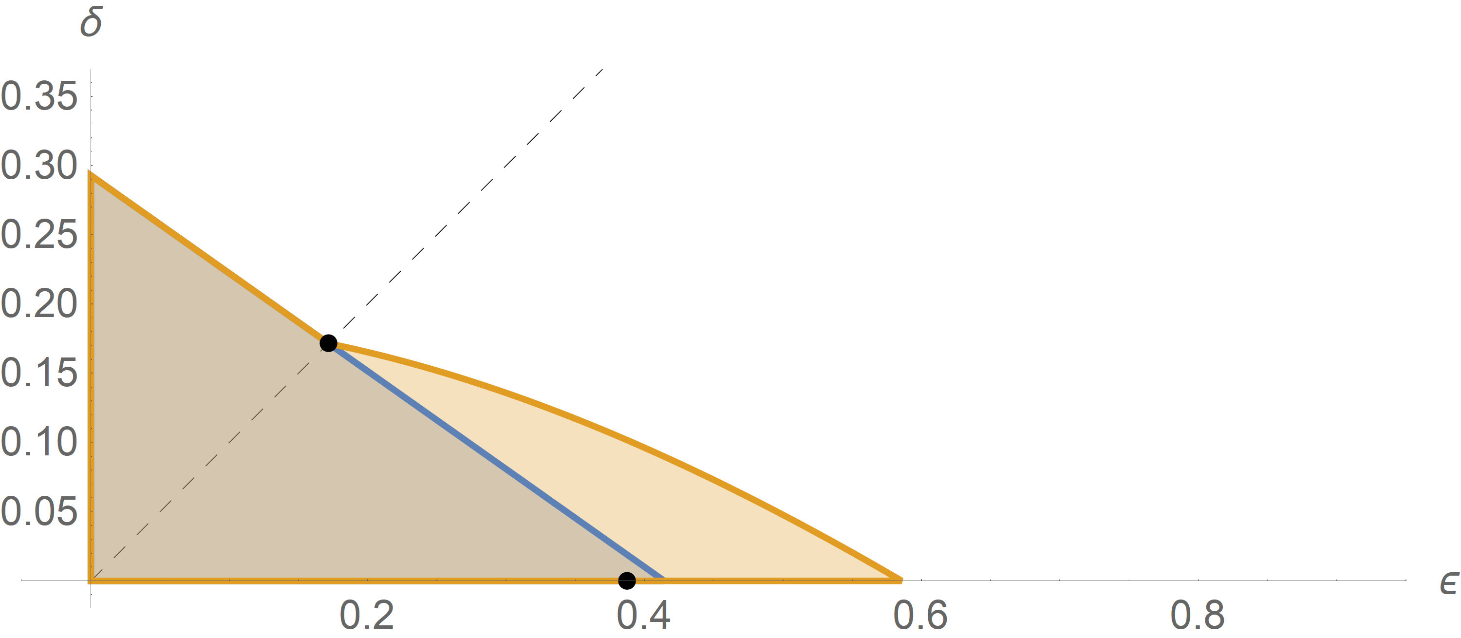
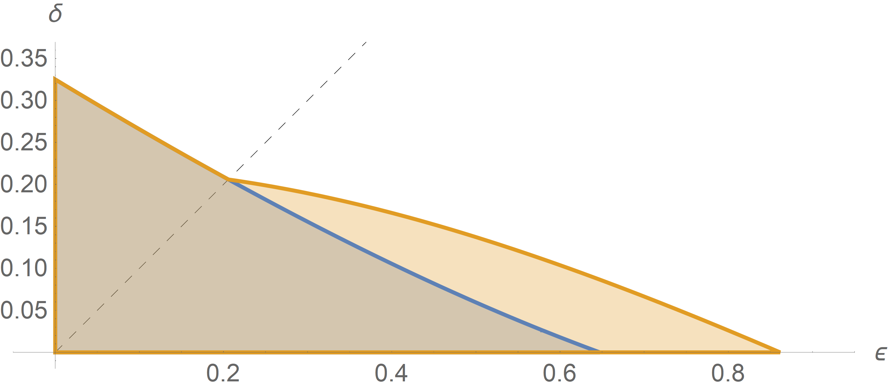
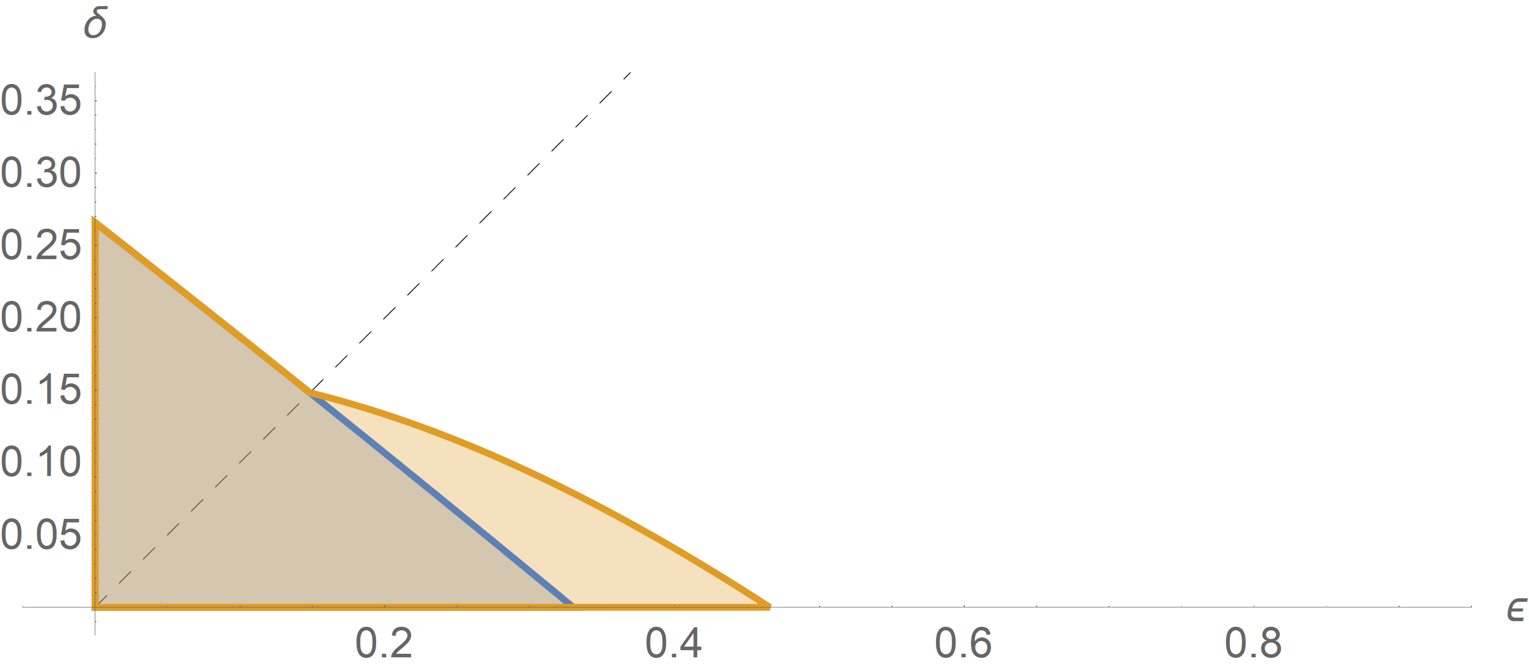
Figure 2: In blue-gray we depict the region in the $(\varepsilon,\delta)$-space for which there exists a radius $r$ such that the union of balls of radius $r$ centred at $P$ captures the homotopy type of a set of positive reach $\mathcal{R}=1$. We do the same in yellow for a manifold of reach $\mathcal{R}=1$. The bounds for the Euclidean setting are indicated on top, for an ambient manifold with positive curvature bound (${\Lambda_{\ell}}=+2$) in the middle, and for an ambient manifold with negative curvature bound (${\Lambda_{\ell}}=-2$) bottom. In the top picture, the black points indicate the bounds that were known to Niyogi, Smale, and Weinberger.

Distinguishing the two one-sided Hausdorff distances seems natural to the authors, because in measurements one would expect the measurement error $\delta$ (with the exception of some small number of outliers) to be often smaller than the sampling density $\varepsilon$. Similar assumptions seem to be common in the learning community, see e.g. [56]. Niyogi, Smale, and Weinberger [61] also made similar assumptions on the support of the measure from which they sampled.

We only consider samples for which we have precise bounds on $\varepsilon$ and $\delta$. In [61], the authors also consider a setting where the point sample is drawn from a distribution centred on the manifold. They still recover the homotopy type of the underlying manifold with high probability. Our results can be applied to improve the bounds also in this context. However, we have not discussed this in detail, since combining both results is straightforward.

We stress that in [21, 61], and [72], the authors use $\varepsilon/2$ instead of our $\varepsilon$. We also stress that $\varepsilon$ and $\delta$ have precisely opposite meanings in [52] compared to this paper.

Our conditions on $\varepsilon$ and $\delta$ are optimal for sets of dimension at least $2$ in the following sense: if the conditions are not satisfied, we can construct a set of positive reach ${\mathcal{S}}$ (resp. manifold $\mathcal{M}$) and a sample $P$, such that there is no $r\geq 0$ for which the union of balls of radius $r$ centred at $P$ would have the same homology as ${\mathcal{S}}$ (resp. $\mathcal{M}$). These constructions are explained in Section 4.4. In the case of $1$-dimensional manifolds, we expect the optimal condition to be weaker.

We would like to emphasize that for noiseless samples, (that is, when $\delta=0$,) both the constant $\left(\sqrt{2}-1\right)$ (for general sets of positive reach), and the constant $\left(2-\sqrt{2}\right)$ (for manifolds) compare favourably with the previously best known constant $\frac{1}{2}\sqrt{\frac{3}{5}}$ from [61] for manifolds.

In Proposition 7.1 of [61], one encounters the condition $\varepsilon<(3-\sqrt{8})\mathcal{R}$ for a particular case of the setting we consider, namely when the sampling condition is expressed through an upper bound $\varepsilon$ on the Hausdorff distance ($\delta=\varepsilon$ in our setting). The same constant $3-\sqrt{8}$ appears independently in [12, Theorem 4] for general sets of positive reach. Our results (Propositions 4.6 and 4.7) show that this bound is optimal when $\delta=\varepsilon$, both for general sets of positive reach and for manifolds.

To contrast the two related results in [61], for $\delta=0$ and $\delta=\varepsilon$ respectively, with our bounds, we portray them as black dots in Figure 2.

Homotopy reconstruction of manifolds with boundary has been studied in [72, Theorem 3.2], assuming lower bounds on both the reach of the manifold and the reach of its boundary. We also improve on this result by treating a manifold with boundary as a particular case of a set of positive reach, while our bounds only depend on the reach of the set itself and not the one of its boundary.

3.2 Subsets of Riemannian manifolds

In the second part of this article we extend the homotopy reconstruction results to sets ${\mathcal{S}}$ and manifolds $\mathcal{M}$ of positive reach embedded in a Riemannian manifold whose sectional curvatures are bounded.

Also in this Riemannian setting we find tight bounds on the one-sided Hausdorff distances $\varepsilon$ and $\delta$ between ${\mathcal{S}}$ (resp. $\mathcal{M}$) and its sample $P$. The set of pairs $(\varepsilon,\delta)$ that satisfy these conditions is depicted in Figure 2 (centre and right). The precise bounds are given in Propositions 5.3 and 5.4.

The main pillar of this part of our work is comparison theory. We recall the most essential definitions and results in Appendix C, and refer to [16, 23, 24, 32, 46, 51] for further reading.

For the extension to the Riemannian setting we also formulate a new generalization of the reach. To establish some of its properties, we use results on the gradient of the distance function [9], see also [57]. These results in turn require non-smooth analysis [34] and semi-concave functions [8]. We refer to Appendix G for discussion.

In computer vision, many papers have argued in favour of using Riemannian manifolds as the main setting without embedding the Riemannian manifold in Euclidean space. In particular, symmetric positive definite matrices and Grassmannians form the natural stage for some data [71, 74]. Symmetric positive definite matrices occur as diffusion tensors [62] (used in e.g. magnetic resonance imaging), in image segmentation [45, 66], and in texture classification [70], while Grassmanians are used in image matching and recognition [47, 48]. Although it is possible to embed these manifolds in Euclidean space, it is not natural and would increase the dimensionality significantly. In [73], time-series obtained from observations of dynamical systems are encoded as positive semi-definite matrices, produced by forming Hankel matrices and taking their Gram matrices. Thus, the problem of analysing time-series data is transformed into the problem of analysing point set data on a Riemannian manifold, namely the one formed by semi-positive definite matrices.

4 Results for subsets of the Euclidean space

4.1 Setting

We denote the closed ball in Euclidean space centred at a point $p$ with radius $r$ by $B(p,r)$.

While working with subsets of the Euclidean space (Section 4 and Appendix A) we assume the following:

For most applications the assumption $\delta\leq\varepsilon$ seems natural, but we do not need this, unless ${\mathcal{S}}=\mathcal{M}$.

4.2 The geometric argument

We show that if the union of balls $P^{\boxplus r}=\bigcup_{p\in P}B(p,r)$ covers a sufficiently large neighbourhood of ${\mathcal{S}}$ and the parameter $r$ is not too big, $P^{\boxplus r}$ deformation-retracts to ${\mathcal{S}}$.

We start by recalling that the normal cone at a point $p$ of a set of positive reach is the set of directions such that if you move in that direction the closest point projection will remain $p$. For a definition we refer to Definition A.2.

Theorem 4.1.

Assume that a parameter $\alpha>0$ is small enough, so that the $\alpha$-neighbourhood ${\mathcal{S}}^{\boxplus\alpha}$ of the set ${\mathcal{S}}$ is contained in $P^{\boxplus r}$. In other words,

$${\mathcal{S}}^{\boxplus\alpha}\subseteq P^{\boxplus r}.$$ (1)

If, moreover,

$$r^{2}\leq(\mathcal{R}-\delta)^{2}-(\mathcal{R}-\alpha)^{2},$$ (2)

then, for any point $q\in{\mathcal{S}}$, the intersection $(q+\mathrm{Nor}(q,{\mathcal{S}}))\cap B(q,\mathcal{R})\cap P^{\boxplus r}$ of the normal cone $q+\mathrm{Nor}(q,{\mathcal{S}})$, the ball $B(q,\mathcal{R})$, and the union of balls $P^{\boxplus r}$, is star-shaped, with the point $q$ as its ‘centre’. Furthermore, $P^{\boxplus r}$ deformation-retracts onto ${\mathcal{S}}$ along the closest point projection.

Remark 4.2.

The statement of Theorem 4.1 does not use the hypothesis ${\mathcal{S}}\subseteq P^{\boxplus\varepsilon}$ from the universal assumption.

We refer to Figure 3 for a pictorial overview of the proof of Theorem 4.1.

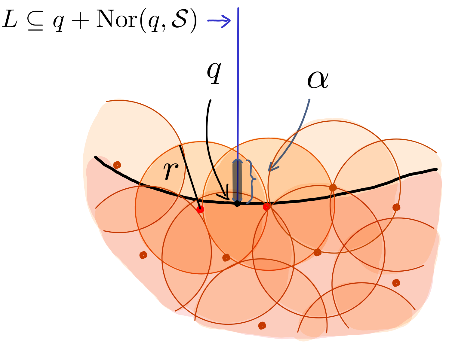
(a) Any point in $q+\mathrm{Nor}(q,{\mathcal{S}})$ a distance less than $\alpha$ from ${\mathcal{S}}$ is covered by $P^{\boxplus r}$.

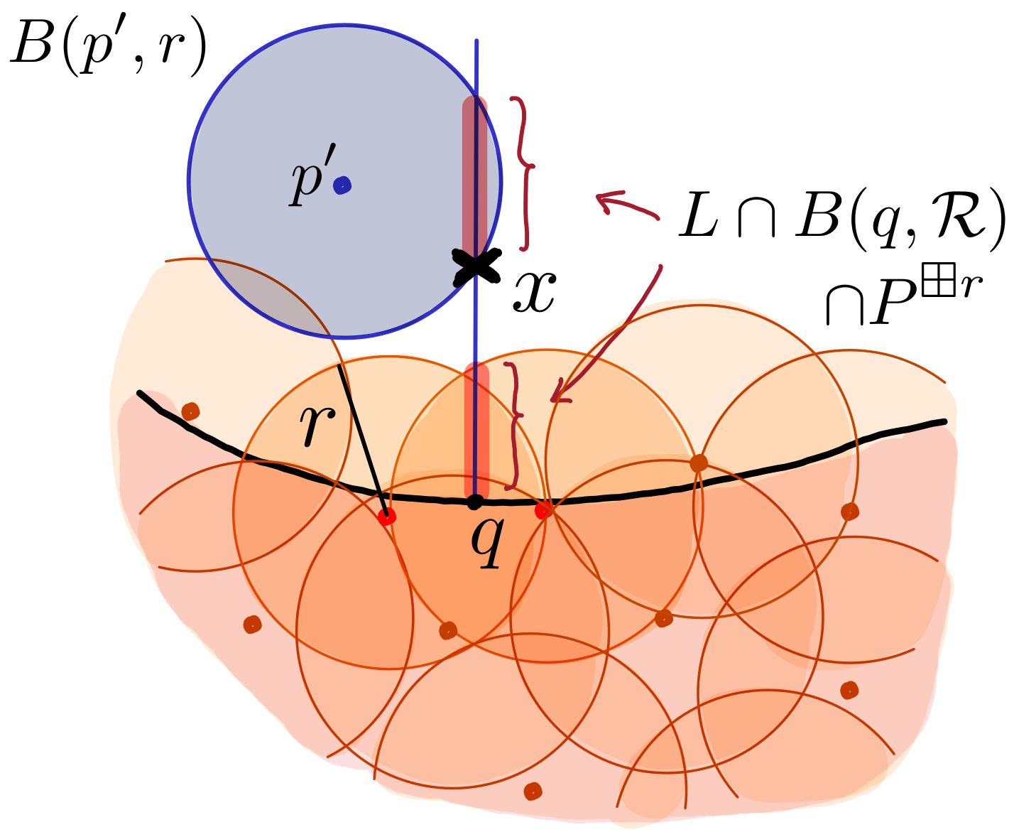
(b) If $(q+\mathrm{Nor}(q,{\mathcal{S}}))\cap P^{\boxplus r}$ is not star-shaped there exists a point $x$ where the segment $L$ reenters a ball $B(p^{\prime},r)$ (in blue) in $P^{\boxplus r}$ after having left $P^{\boxplus r}$ closer to $q$.

(c) The centre $p^{\prime}$ of the ball $B(p^{\prime},r)$ lies inside the half space $H$. The half space $H$ lies at least a distance $\alpha$ from $q$.

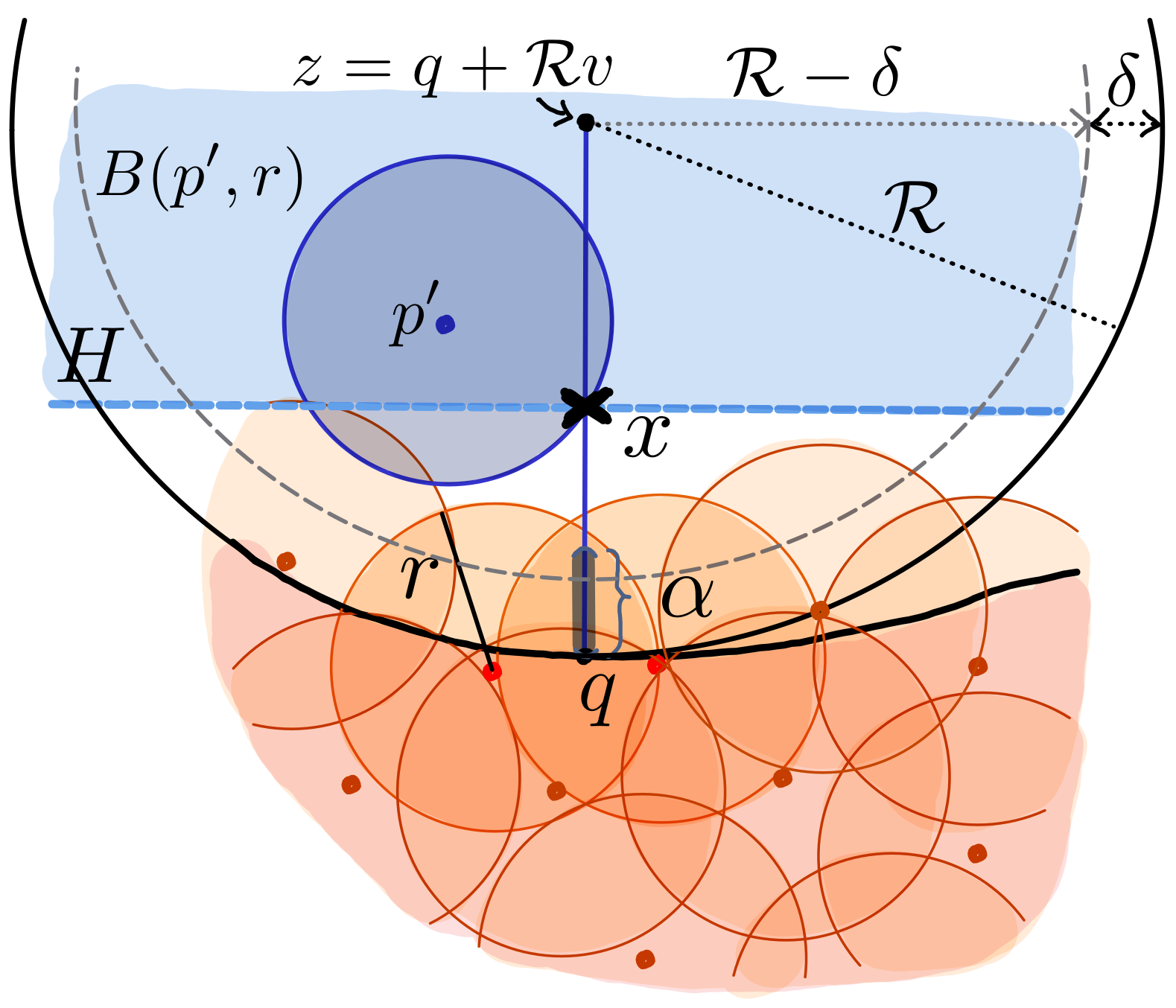
(d) The ball of radius $\mathcal{R}$ is ‘tangent’ to the set ${\mathcal{S}}$, thus it cannot contain any point of ${\mathcal{S}}$ in its interior. Since the distance between $p^{\prime}$ and ${\mathcal{S}}$ is bounded by $\delta$, $p^{\prime}$ has to lie outside of the ball of radius $\mathcal{R}-\delta$. This contradicts the fact that $p^{\prime}$ lies in the halfspace $H$ and is not too far from the normal space $q+\mathrm{Nor}(q,{\mathcal{S}})$.

Figure 3: A pictorial overview of the proof. The pink shaded region represents a part of the set ${\mathcal{S}}$, the union of balls $P^{\boxplus r}$ is coloured orange. The thickened blue segment shows those points of the segment $L$ that lie a distance less than $\alpha$ from ${\mathcal{S}}$. Per assumption, this segment is contained in the union of balls $P^{\boxplus r}$.

Proof 4.3 (Proof of Theorem 4.1).

We prove the claim by contradiction. For any point $q\in{\mathcal{S}}$, the set $(q+\mathrm{Nor}(q,{\mathcal{S}}))\cap\left({\mathcal{S}}^{\boxplus\alpha}\right)$ is contained in the union of balls $P^{\boxplus r}$. In Figure 3(a), we illustrate this for the case where the set $q+\mathrm{Nor}(q,{\mathcal{S}})$ consists of one ray. Assume that there exists a point $q\in{\mathcal{S}}$ and a vector $v\in\mathrm{Nor}(q,{\mathcal{S}})$, with $\|v\|=1$, such that the intersection of $P^{\boxplus r}$ with the segment

$$L\underset{\text{def.}}{=}\>\{q+\lambda v\mid\lambda\in[0,\mathcal{R})\}$$

consists of several connected components (as illustrated in Figure 3(b)). Thanks to Equation (1), the connected component that contains $q$ has length at least $\alpha$. Let $x$ be first point along $L$, seen from $q$, lying inside a connected component of $\left(P^{\boxplus r}\right)\cap L$ that does not contain $q$. Then $x$ lies at the intersection of the segment $L$ and a ball $B(p^{\prime},r)$, with $p^{\prime}\in P$. Furthermore, the point $p^{\prime}$ is contained in the open half space $H$ orthogonal to the vector $v$, that does not contain $q$, and whose boundary contains $x$. We stress that if $p^{\prime}$ lies on the boundary of $H$ then the line $L$ is tangent to the sphere $\partial B(p^{\prime},r)$, which is still compatible with star-shapedness. The situation is illustrated in Figure 3(c).

Let $z=q+\mathcal{R}v$ be the open endpoint of $L$. Since, by Theorem A.5 ([41, Theorem 4.8 (12)]), the intersection ${\mathcal{S}}\cap B(z,\mathcal{R})^{\circ}$ is empty and the distance between $p^{\prime}$ and ${\mathcal{S}}$ is bounded by $\delta$, we know that $p^{\prime}\notin B(z,\mathcal{R}-\delta)^{\circ}$. Thus,

$$p^{\prime}\in A\underset{\text{def.}}{=}\>H\cap(\mathbb{R}^{d}\setminus B(z,\mathcal{R}-\delta)^{\circ}).$$

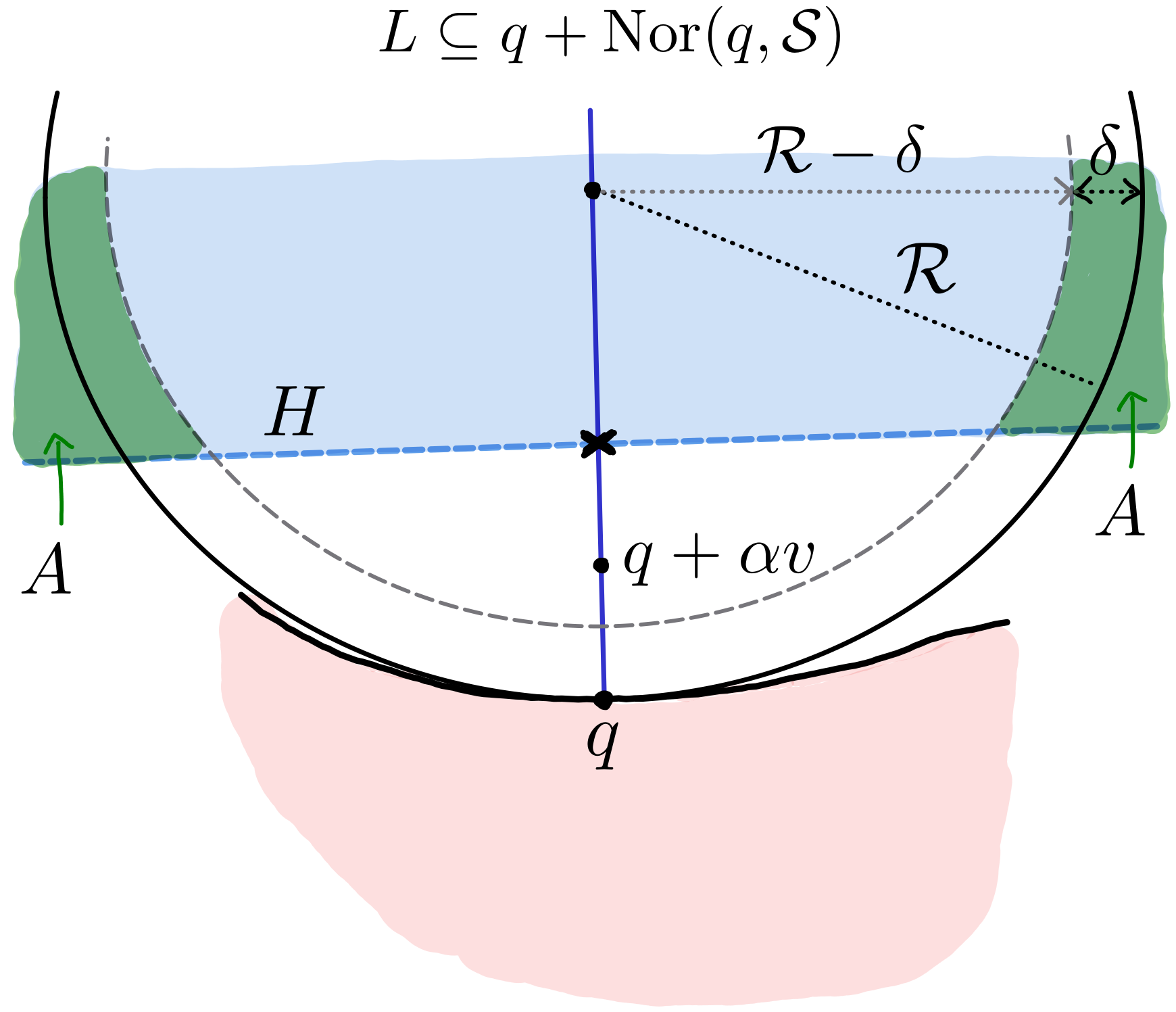
Figure 4: We depict the extremal case where $x=q+\alpha v$. The centre of the ball creating a new connected component along one direction in the normal cone $q+\mathrm{Nor}(q,{\mathcal{S}})$ (in blue) is constrained to belong to the set $A$ (in green). The set ${\mathcal{S}}$ is coloured pink, the halfplane $H$ in light blue.

The sphere $\partial B(z,\mathcal{R}-\delta)$ has a non-empty intersection with the plane $\partial H$. Indeed, the sphere passes through point $q+\delta v$ which does not belong to $H$ while its centre $z$ belongs to $H$; see Figure 3(d). We can thus pick a point $y$ in the intersection $\partial H\cap\partial B(z,\mathcal{R}-\delta)$. By the Pythagorean theorem, the minimal squared distance between $A$ and $L$ is:

$$\inf_{\begin{subarray}{c}a\in A\\ \ell\in L\end{subarray}} \|a-\ell\|^{2}=\|x-y\|^{2}=\|z-y\|^{2}-\left(\|z-q\|-\|x-q\|\right)^{2}\geq(\mathcal{R}-\delta)^{2}-(\mathcal{R}-\alpha)^{2},$$

as illustrated in Figure 4. Hence, if

$$r^{2}\leq(\mathcal{R}-\delta)^{2}-(\mathcal{R}-\alpha)^{2},$$ (2)

the ball $B(p^{\prime},r)$ does not intersect $L$. Therefore, $L\cap(P^{\boxplus r})$ cannot have more than one connected component. The set $(q+\mathrm{Nor}(q,{\mathcal{S}}))\cap B(q,\mathcal{R})\cap(P^{\boxplus r})$ is thus star-shaped with centre $q$.

Since $r$ satisfies Equation (2), we deduce that $\delta+r<\mathcal{R}$, and thus

$$P^{\boxplus r}\subseteq\left({\mathcal{S}}^{\boxplus\mathcal{R}}\right)^{\circ}.$$

Thanks to this, the fact that the set $(q+\mathrm{Nor}(q,{\mathcal{S}}))\cap B(q,\mathcal{R})\cap(P^{\boxplus r})$ is star-shaped with centre $q$, and Theorem A.5, the map

$$\mathcal{H}: [0,1]\times(P^{\boxplus r})\to P^{\boxplus r},$$

$$(t,x)\mapsto(1-t)x+t\pi_{{\mathcal{S}}}(x),$$

is well-defined.

Furthermore, since ${\mathcal{S}}$ has positive reach, then, thanks to Theorem A.4 ([41, Theorem 4.8 (8)]), the projection $\pi_{{\mathcal{S}}}$ is (Lipschitz) continuous. Thus, the map $\mathcal{H}$ is a deformation retract from the union of balls $P^{\boxplus r}$ to the set ${\mathcal{S}}$.

In Appendix E, we provide an alternative proof of Theorem 4.1, similar to an argument presented in [30].

4.3 Bounds on the sampling parameters

For sets of positive reach, we obtain the following bounds on $\varepsilon$ and $\delta$:

Proposition 4.4.

If $\varepsilon$ and $\delta$ satisfy

$$\varepsilon+\sqrt{2}\,\delta\leq(\sqrt{2}-1)\mathcal{R},$$ (3)

there exists a radius $r>0$ such that the union of balls $P^{\boxplus r}=\bigcup_{p\in P}B(p,r)$ deformation-retracts onto ${\mathcal{S}}$ along the closest point projection. In particular, $r$ can be chosen as:

$$r\in\left[\frac{1}{2}\left(\mathcal{R}+\varepsilon-\sqrt{\Delta}\right),\frac{1}{2}\left(\mathcal{R}+\varepsilon+\sqrt{\Delta}\right)\right],$$ (4)

where $\Delta=2(\mathcal{R}-\delta)^{2}-(\mathcal{R}+\varepsilon)^{2}$.

If the set is a manifold, the bounds on $\varepsilon$ and $\delta$ can be improved as follows:

Proposition 4.5.

If $\varepsilon$ and $\delta$ satisfy

$$(\mathcal{R}-\delta)^{2}-\varepsilon^{2}\geq\left(4\sqrt{2}-5\right)\mathcal{R}^{2}$$ (5)

and $\delta\leq\varepsilon$, there exists a radius $r>0$ such that the union of balls $P^{\boxplus r}$ deformation-retracts onto $\mathcal{M}$ along the closest point projection. The radius $r$ can be chosen as in (18).

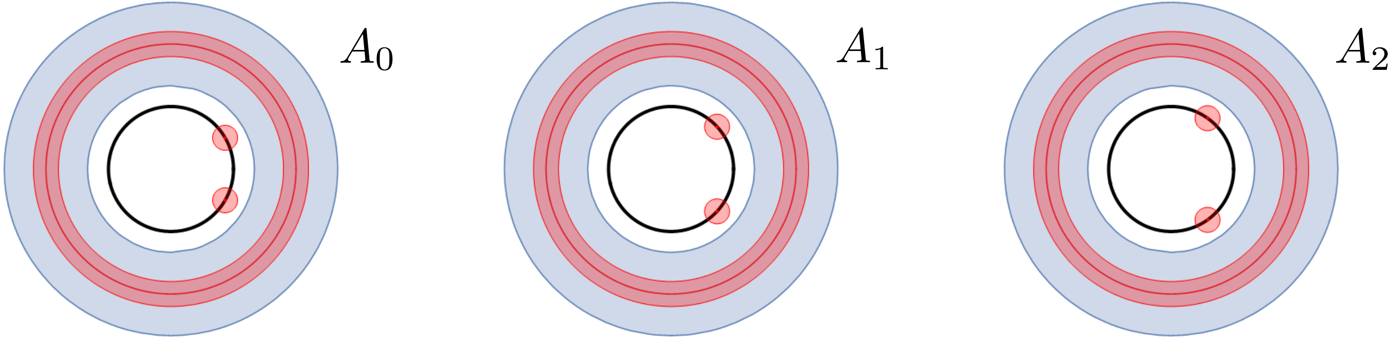
(a) At first, the thickening of the sample has three connected components per annulus. The thickening thus has three times as many connected components as the set ${\mathcal{S}}$.

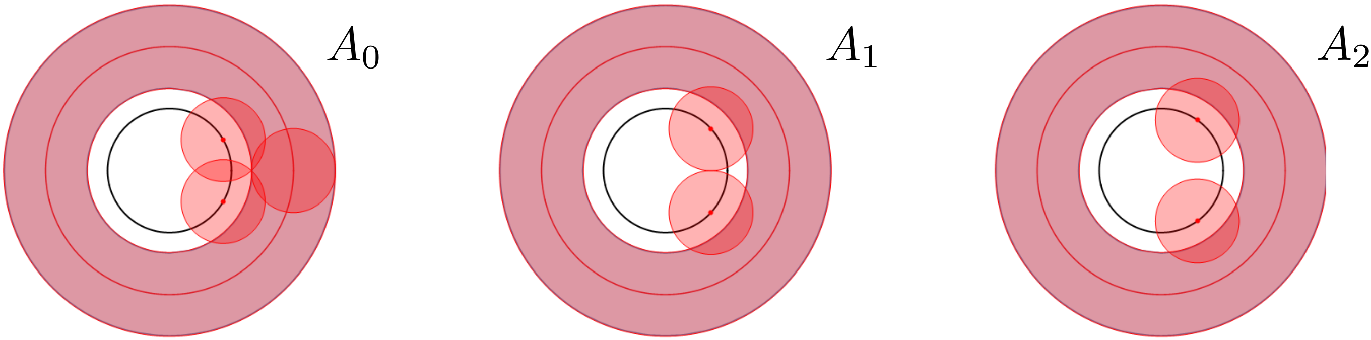
(b) As the radius of the thickening grows, the connected components merge. However, at all times there exists an additional cycle at one of the annuli (annulus $A_{1}$ in this case).

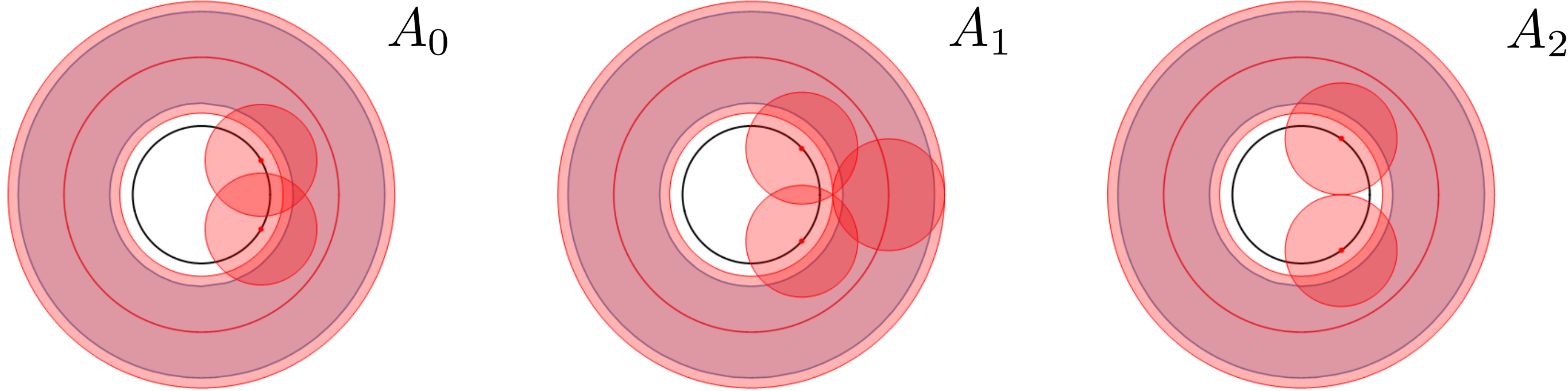
(c) At the moment when the cycle at annulus $A_{1}$ vanishes, another cycle is formed at annulus $A_{2}$.

Figure 5: A pictorial explanation of why $P^{\boxplus r}$ never has the homotopy type of the set ${\mathcal{S}}$. We only depict three annuli in the sequence of $A_{i}$s. The set ${\mathcal{S}}$ is in blue, the sample $P$ in red, and the thickening of $P$ in pink. The black circles indicate the location of the two isolated sample points of $P$ associated to each annulus.

4.4 Tightness of the bounds on the sampling parameters

Our sampling criteria for homotopy inference of sets of positive reach are tight in the following sense:

Proposition 4.6.

Suppose that the dimension $d$ of the ambient space $\mathbb{R}^{d}$ satisfies $d\geq 2$, and the one-sided Hausdorff distances $\varepsilon$ and $\delta$ fail to satisfy bound (3). Then there exists a set ${\mathcal{S}}$ of positive reach and a sample $P$ that satisfy Universal Assumption 4.1, while the homology of the union of balls $P^{\boxplus r}$ does not equal the homology of ${\mathcal{S}}$ for any $r$.

We construct the set ${\mathcal{S}}$ and the sample $P$ explicitly. The set ${\mathcal{S}}$ consists of annuli $A_{i}$ and the sample $P$ is the union of a circle and two points for every annulus. In Figure 5, we illustrate that the thickening of the sample never captures the homotopy type of the set ${\mathcal{S}}$. The details of the construction and the proof of Proposition 4.6 are provided in Section A.3.1.

Figure 6: The (half of the) torus $T_{i}$ depicted in blue; the sample — the set $C_{i}$ and the points $p_{i}$ and $\tilde{p}_{i}$ — in red. In black we indicate the circle $C^{\prime}_{i}$ on which the points $p_{i}$ and $\tilde{p}_{i}$ lie. The closest point projection of this circle onto $\mathcal{M}$ is indicated in blue.

Proposition 4.7.

Suppose that the dimension $d$ of the ambient space $\mathbb{R}^{d}$ satisfies $d\geq{3}$, the one-sided Hausdorff distances $\varepsilon$ and $\delta$ fail to satisfy bound (5), and $\delta\leq\varepsilon$. Then there exists a manifold $\mathcal{M}$ of positive reach and a sample $P$ that satisfy Universal Assumption 4.1, while the homology of the union of balls $P^{\boxplus r}$ does not equal the homology of $\mathcal{M}$ for any $r$.

We again construct the manifold $\mathcal{M}$ and the sample $P$ explicitly. The manifold $\mathcal{M}$ is a union of tori. The sample $P$ consists of sets $C_{i}$ which are tori (the ‘interior’ part of the $\delta$ offset of $\mathcal{M}$) with a part cut out, and pairs of points $\{p_{i},\tilde{p}_{i}\}$. We illustrate the manifold $\mathcal{M}$ together with the sample $P$ in Figure 6, and sketch why the underlying homology is not captured in Figure 7. The proof of Proposition 4.7 as well as details on the construction are provided in Section A.3.2.

(a) At first, the balls around the points $p_{i}$ and $\tilde{p}_{i}$ do not intersect the thickening of the set $C_{i}$, and thus the number of connected components of the thickening (in pink) of $P$ is different from the number of components of the manifold.

(b) Then we create a (or possibly multiple) spurious cycle(s) for the first torus in the sequence (on the left).

(c) By the time the spurious cycles at the first torus have disappeared, others have been created at the second torus. This process is then repeated for all tori in the sequence as $r$ increases.

Figure 7: The construction for manifolds imitates the construction for general sets of positive reach as much as possible. The manifold $\mathcal{M}$ is depicted in blue, the sample $P$ in red, and the thickening in pink. We only display the part of objects below a horizontal clipping plane.

Remark 4.8.

For simplicity, the sets constructed, see Figures 7 and 5 (or Examples A.19 and A.23 in the appendix for details), are not connected. However, in each construction one can glue the connected components together in a way that preserves the reach, and the resulting examples still yield Propositions 4.6 and 4.7. See Figure 8 for a sketch of the modification needed.

        

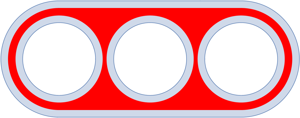
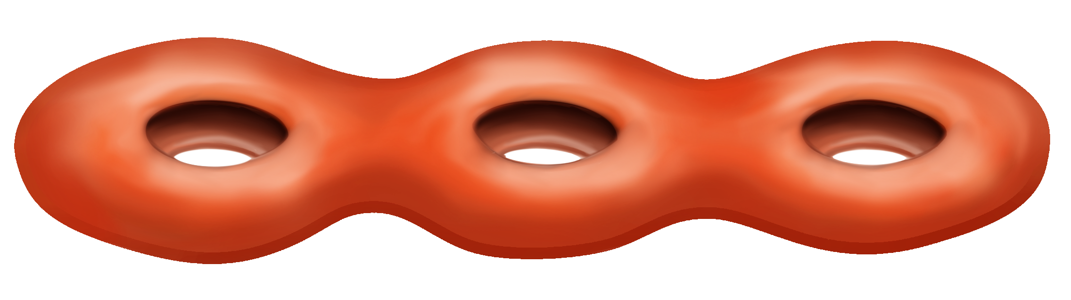
Figure 8: The connected variants of our sets ${\mathcal{S}}$ and $\mathcal{M}$ are a topological disc with $k$ holes and a genus $k$ surface. On the left we sketch both the sample and the set of positive reach, on the right we only give the sample for the manifold setting because of visualization constraints.

5 Results for subsets of Riemannian manifolds

5.1 Setting

In the second part of this paper we consider subsets of a ($C^{2}$) Riemannian manifold $\mathcal{N}$. setting we denote balls with radius $r>0$ centred at a point $p\in\mathcal{N}$ by $B(p,r)$, and write $A^{\boxplus r}=\bigcup_{a\in A}B(a,r)$ for the union of balls of radius $r$ centred at a subset $A\subseteq\mathcal{N}$.

To be able to proceed as in the Euclidean setting and state tight bounds on the sampling parameters, we need a notion of the reach in the Riemannian setting. To this end, we introduce a new definition, inspired by the cut locus (which is defined for example in [16]):

Definition 5.1 (Cut locus).

Given a closed subset ${\mathcal{S}}\subseteq\mathcal{N}$, the cut locus of ${\mathcal{S}}$ is the set $\operatorname{cl}_{\mathcal{N}}({\mathcal{S}})$ of points $p\in\mathcal{N}$ for which there are at least $2$ geodesics of minimal length from $p$ to some point in ${\mathcal{S}}$.

Definition 5.2 (Cut locus reach).

The cut locus reach $\mathrm{rch}^{\operatorname{cl}}_{\mathcal{N}}({\mathcal{S}})$ of a closed set ${\mathcal{S}}\subseteq\mathcal{N}$ is the infimum of distances between ${\mathcal{S}}$ and its cut locus $\operatorname{cl}_{\mathcal{N}}({\mathcal{S}})$:

$$\mathrm{rch}^{\operatorname{cl}}_{\mathcal{N}}({\mathcal{S}})\underset{\text{def.}}{=}\>\inf_{\begin{subarray}{c}p\in{\mathcal{S}},\\ q\in\operatorname{cl}_{\mathcal{N}}({\mathcal{S}}),\end{subarray}}d_{\mathcal{N}}(p,q).$$

Our definition is a refinement of the notion used by Bangert and Kleinjohann [14, 53, 54], as well as the reach defined in [22]. We explain why our new definition is appropriate for the learning of topological features in Appendix F. Using the new extension of the reach we assume the following conditions, which resemble the ones in the Euclidean setting closely:

This assumption is used in Section 5 and Appendix B.

5.2 Bounds on the sampling parameters

Also in the Riemannian setting we provide (tight) bounds that the sample $P$ needs to satisfy in order to be able to infer homotopy. For sets of positive (cut locus) reach, we obtain the following bounds on $\varepsilon$ and $\delta$:

Proposition 5.3.

If $\varepsilon$ and $\delta$ satisfy

$$2\cos\left(\sqrt{{\Lambda_{\ell}}}(\mathcal{R}-\delta)\right)-\cos\left(\sqrt{{\Lambda_{\ell}}}(\mathcal{R}+\varepsilon)\right) \leq 1 {\Lambda_{\ell}}>0$$ if

$$\varepsilon+\sqrt{2}\,\delta \leq(\sqrt{2}-1)\mathcal{R}, \text{if ${\Lambda_{\ell}}=0$},$$ (6)

$$2\cosh\left(\sqrt{{{\left\lvert{\Lambda_{\ell}}\right\rvert}}}(\mathcal{R}-\delta)\right)-\cosh\left(\sqrt{{{\left\lvert{\Lambda_{\ell}}\right\rvert}}}(\mathcal{R}+\varepsilon)\right) \geq 1 \text{if ${\Lambda_{\ell}}<0$},$$

there exists a radius $r>0$ such that the union of balls $P^{\boxplus r}$ deformation-retracts onto ${\mathcal{S}}$ along the closest point projection. In particular, $r$ can be chosen as:

$$r=\frac{1}{2}\left(\mathcal{R}+\varepsilon\right).$$ (7)

If the set is a manifold, the bounds on $\varepsilon$ and $\delta$ can be improved as follows:

Proposition 5.4.

Let $\tilde{x}=\sqrt{{{\left\lvert{\Lambda_{\ell}}\right\rvert}}}x$. For $\delta\leq\varepsilon$ satisfying

$$\left(2\cos\tilde{\varepsilon}\cos\tilde{\mathcal{R}}-3\cos\left(\tilde{\mathcal{R}}-\tilde{\delta}\right)\right)^{2}\leq\left(\frac{\cos\tilde{\varepsilon}-\cos\left(\tilde{\mathcal{R}}-\tilde{\delta}\right)\cos\tilde{\mathcal{R}}}{\sin\tilde{\mathcal{R}}}\right)^{2}+\cos^{2}\left(\tilde{\mathcal{R}}-\tilde{\delta}\right)$$

$$\hskip 341.43306pt\textrm{\emph{if ${\Lambda_{\ell}}>0$}},$$ (8)

$$(\mathcal{R}-\delta)^{2}-\varepsilon^{2}\geq\left(4\sqrt{2}-5\right)\mathcal{R}^{2}\hskip 193.47882pt\textrm{\emph{if ${\Lambda_{\ell}}=0$}},$$ (5)

$$2\cosh\tilde{\varepsilon}\cosh\tilde{\mathcal{R}}\leq 3\cosh\left(\tilde{\mathcal{R}}-\tilde{\delta}\right)\qquad\text{and}\qquad$$

$$\cosh^{2}\left(\tilde{\mathcal{R}}-\tilde{\delta}\right)\leq\left(\frac{\cosh\tilde{\varepsilon}-\cosh\left(\tilde{\mathcal{R}}-\tilde{\delta}\right)\cosh\tilde{\mathcal{R}}}{\sinh\tilde{\mathcal{R}}}\right)^{2}+\left(2\cosh\tilde{\varepsilon}\cosh\tilde{\mathcal{R}}-3\cosh\left(\tilde{\mathcal{R}}-\tilde{\delta}\right)\right)^{2}$$

$$\hskip 341.43306pt\textrm{\emph{if ${\Lambda_{\ell}}<0$}},$$ (9)

there exists a radius $r>0$ such that $P^{\boxplus r}$ deformation-retracts onto $\mathcal{M}$ along the (geodesic) closest point projection $\pi_{\mathcal{M}}$. The interval from which $r$ can be chosen can be recovered from (41), (18), and (44) respectively.

5.3 Tightness of the bounds on the sampling parameters

We exhibit the tightness of the bounds on $\varepsilon$ and $\delta$ from Propositions 5.3 and 5.4 by constructions of examples in (simply connected) spaces of constant curvature. These constructions are similar to the Euclidean setting — they also consist of annuli and tori, see Figure 9. However, due to the curvature of the ambient manifold, the proof of the tightness of the bounds is significantly more involved (see Appendix B.4).

Figure 9: The construction for sets of positive reach on a manifold with (constant) positive curvature (the sphere). For a detailed version of the figure see Figure 23.

6 Future work

This article leaves several important questions unanswered. We mention three.

First of all, we consider the union of balls centered on a sample $P$ whose homotopy type is equal to that of the Čech complex of $P$ and, when the ambient space is a Riemannian manifold, the radius of balls is smaller than the convexity radius.

It would be interesting to see if our work would help understanding the same question for Rips complexes. For related work see e.g. [6, 7, 49, 55].

Second, we consider sets embedded in Riemannian manifolds whose sectional curvature is lower bounded. A natural question is under which conditions do our results generalize to a larger class of metric spaces with lower bounded curvatures.

The generalized gradient of the distance function and its flow have been used to generalize results on subsets of positive reach in Euclidean space to subsets with positive $\mu$-reach and weak feature size [25, 26, 29, 31]. Our work on the cut locus reach makes it possible to extend the notations of positive $\mu$-reach and weak feature size to Riemannian manifolds. It is expected that many of the main results from the Euclidean setting still hold with minor modifications in this more general context.

Appendix I: The technical statements and proofs

The two sections in this part of our paper are structured in the same way. In the first section (Section A), we deal with subsets of Euclidean space, in the second (Section B) with subsets of Riemannian manifolds. In each section, we first introduce necessary definitions and recall the general setting (Sections A.1 and B.1). In Sections 4.2 and B.2 we consider a set ${\mathcal{S}}$, its sample $P$, and use a geometric argument to establish a condition on the thickening parameter $r>0$ that guarantees that the thickening $P^{\boxplus r}$ of the sample $P$ deformation-retracts to the set ${\mathcal{S}}$. In the following sections (Sections A.2 and B.3) we show that if the sampling parameters $\varepsilon$ and $\delta$ of the sample satisfy certain bounds, the condition on the thickening parameter is never satisfied. We carefully distinguish between subsets (Sections A.2.1 and B.3.1) and submanifolds (Sections A.2.2 and B.3.2), for which we obtain sharper bounds. Finally (Sections A.3 and B.4), we construct explicit counterexamples to prove that our bounds on the sampling parameters are tight.

Appendix A Subsets of the Euclidean space

A.1 Definitions and setting

In this section we revise the notions and results by Federer [41]. We assume that ${\mathcal{S}}\subset\mathbb{R}^{d}$ is a closed set, and denote the closest point projection on ${\mathcal{S}}$ by $\pi_{\mathcal{S}}$.

At first, we define the medial axis, the local feature size, and the reach of the set ${\mathcal{S}}$:

Definition A.1.

The medial axis $\operatorname{{ax}}({\mathcal{S}})$ of a set ${\mathcal{S}}$ is the set of points in the ambient Euclidean space that do not have a unique closest point on ${\mathcal{S}}$. The distance from a point $p$ to the medial axis is called the local feature size $\mathrm{lfs}(p)$. Finally, the (minimal) distance between $\operatorname{{ax}}({\mathcal{S}})$ and ${\mathcal{S}}$ is the reach $\mathrm{rch}({\mathcal{S}})$ of ${\mathcal{S}}$:

$$\mathrm{lfs}(p)=\inf_{q\in\operatorname{{ax}}({\mathcal{S}})}\left\|{p-q}\right\|,\qquad\mathrm{rch}({\mathcal{S}})=\inf_{p\in{\mathcal{S}}}\mathrm{lfs}(p).$$

For example, the medial axis of an ellipse in the Euclidean plane is the (open) segment connecting the two focal points, and the reach is the distance from (one of) the focal point(s) to the ellipse.

Next, we introduce the normal cone. We denote the scalar product in $\mathbb{R}^{d}$ by $\langle.,.\rangle$.

Definition A.2 (Definitions 4.3 and 4.4 of [41]).

If ${\mathcal{S}}\subseteq\mathbb{R}^{d}$ and $p\in{\mathcal{S}}$, then the generalized tangent space $\mathrm{Tan}(p,{\mathcal{S}})$ is the set of all tangent vectors of ${\mathcal{S}}$ at $p$. It consists of all those $u\in\mathbb{R}^{d}$, such that either $u=0$ or for every $\varepsilon>0$ there exists a point $q\in{\mathcal{S}}$ with

$$0< \|q-p\|<\varepsilon \left\|\frac{q-p}{\|q-p\|}-\frac{u}{\|u\|}\right\|<\varepsilon.$$ and

The normal cone of ${\mathcal{S}}$ at $p$ is the set

$$\mathrm{Nor}(p,{\mathcal{S}})$$

of all vectors $v\in\mathbb{R}^{d}$ such that $\langle v,u\rangle\leq 0$ for all $u\in\mathrm{Tan}(p,{\mathcal{S}})$.

We illustrate the medial axis and a few normal cones in Figure 1 (left). The normal cone is indeed a cone, geometrically speaking:

Definition and Remark A.3 ([41, Remark 4.5]).

A subset $C\subseteq\mathbb{R}^{d}$ is a convex cone if and only if for all $x,y\in C$ and $\lambda>0$ we have $x+y\in C$ and $\lambda x\in C$. For every set $A\subseteq\mathbb{R}^{d}$, its dual

$$\mathrm{Dual}(A)=\{v\mid\langle v,u\rangle\leq 0\textrm{ for all }u\in A\},$$

is a closed convex cone. The double dual, $\mathrm{Dual}(\mathrm{Dual}(A))$, is the smallest closed convex cone that contains the set $A$. The set $\mathrm{Nor}(p,{\mathcal{S}})$ is therefore a convex cone.

The generalized tangent space $\mathrm{Tan}(p,{\mathcal{S}})$, on the other hand, is only closed and positively homogeneous, but not necessarily convex. That is, if $v\in\mathrm{Tan}(p,{\mathcal{S}})$, $\lambda v\in\mathrm{Tan}(p,{\mathcal{S}})$ for all $\lambda\in\mathbb{R}_{\geq 0}$. The space $\mathrm{Tan}(p,{\mathcal{S}})$ is a convex cone if the set ${\mathcal{S}}$ has positive reach, as we will see below.

With these definitions in place we present the following two theorems, that form the core of the proof of our statement on deformation retraction of the set ${\mathcal{S}}$ (Theorem 4.1).

Theorem A.4 ([41, Theorem 4.8 (8)]).

Let $\ell$ and $\mathcal{R}$ satisfy $0<\ell<\mathcal{R}<\infty$ and $\mathrm{rch}({\mathcal{S}})\geq\mathcal{R}$. Then any points $x,y\in\mathbb{R}^{d}\backslash\operatorname{{ax}}({\mathcal{S}})$ with

$$d(x,{\mathcal{S}})\leq\ell\qquad\text{and}\qquad d(y,{\mathcal{S}})\leq\ell$$

satisfy

$$\|\pi_{\mathcal{S}}(x)-\pi_{\mathcal{S}}(y)\|\leq\frac{\mathcal{R}}{\mathcal{R}-\ell}\|x-y\|.$$

Theorem A.5 ([41, Theorem 4.8 (12)]).

Let $p\in{\mathcal{S}}$. Then for any number $\ell$ satisfying $\mathrm{lfs}(p)>\ell>0$, the normal cone equals

$$\mathrm{Nor}(p,{\mathcal{S}})=\{\lambda v\mid\lambda\geq 0,\|v\|=\ell,\pi_{{\mathcal{S}}}(p+v)=p\}.$$

$\mathrm{Tan}(p,{\mathcal{S}})$ is the convex cone dual to $\mathrm{Nor}(p,{\mathcal{S}})$, and, for any vector $u\in{\mathrm{Tan}(p,{\mathcal{S}})}$,

$$\lim_{t\to 0^{+}}t^{-1}d(p+tu,{\mathcal{S}})=0.$$

Finally, we recall the setting we assume for the remainder of Section A:

A.2 Bounds on the sampling parameters

In this section we first compute the bounds on the size $\alpha$ of the neighbourhood ${\mathcal{S}}^{\boxplus\alpha}$ covered by the union of balls $\bigcup_{p\in P}B(p,r)=P^{\boxplus r}$ in terms of $\varepsilon,\delta$, and $r$. We then combine these bounds with Equation (2) to infer (optimal) upper bounds on $\varepsilon$ and $\delta$, for which there exists a radius $r$ such that the deformation retract from $P^{\boxplus r}$to ${\mathcal{S}}$ is possible. We do so first for sets of positive reach and then for manifolds. Somewhat counter-intuitively, it turns out to be easier to determine the bounds for sets of positive reach.

A.2.1 Sets of positive reach

For sets of positive reach, the bound on $\alpha$ is almost trivial. Nevertheless, it is tight, as we will see in Section A.3.

Lemma A.6.

Suppose that ${\mathcal{S}}\subseteq P^{\boxplus\varepsilon}$ for some $\varepsilon\geq 0$. Then, for all $\alpha\leq r-\varepsilon$, the $\alpha$-neigbourhood ${\mathcal{S}}^{\boxplus\alpha}$ of ${\mathcal{S}}$ is contained in the union of balls $P^{\boxplus r}$. That is,

$${\mathcal{S}}^{\boxplus\alpha}\subseteq P^{\boxplus r}.$$

Proof A.7.

Writing out the definition we see that the $\boxplus$ operation is additive. For any set $A\subseteq\mathbb{R}^{d}$:

$$(A^{\boxplus r_{1}})^{\boxplus r_{2}} =\bigcup_{a^{\prime}\in A^{\boxplus r_{1}}}B(a^{\prime},r_{2})$$

$$=\bigcup_{a^{\prime}\in\bigcup_{a\in A}B(a,r_{1})}B(a^{\prime},r_{2})$$

$$\subseteq\bigcup_{a\in A}B(a,r_{1}+r_{2})$$ (by the triangle inequality)

$$=A^{\boxplus(r_{1}+r_{2})}.$$ (10)

So indeed,

$${\mathcal{S}}^{\boxplus\alpha} \subseteq(P^{\boxplus\varepsilon})^{\boxplus\alpha} {\mathcal{S}}\subseteq P^{\boxplus\varepsilon}$$ (because )

$$\subseteq P^{\boxplus(\varepsilon+\alpha)}$$ (by (10))

$$\subseteq P^{\boxplus r}. \alpha\leq r-\varepsilon$$ (because by assumption )

Remark A.8.

The statement of Lemma A.6 holds in any metric space. Writing $B(a,r)$ for a metric ball with radius $r$ centred at a point $a$, and $A^{\boxplus r}=\bigcup_{a\in A}B(a,r)$ for the thickening of a set $A$ in the metric space, we see from the proof of Lemma A.6 that

$$(A^{\boxplus r_{1}})^{\boxplus r_{2}}\subseteq A^{\boxplus(r_{1}+r_{2})},$$

with equality if the metric space is geodesic.

From Lemma A.6, we derive the bounds on $\varepsilon$ and $\delta$ (in terms of $\mathcal{R}$).

See 4.4

Proof A.9.

We combine the bound from Lemma A.6 with the conditions of Theorem 4.1. More precisely, inserting $\alpha=r-\varepsilon$ in Equation (2) yields that

$$r^{2}+(\mathcal{R}-r+\varepsilon)^{2}\leq(\mathcal{R}-\delta)^{2}.$$ (11)

Using the abc-formula for quadratic equations, this is equivalent to

$$r\in\left[\frac{1}{2}\left(\mathcal{R}+\varepsilon-\sqrt{\Delta}\right),\frac{1}{2}\left(\mathcal{R}+\varepsilon+\sqrt{\Delta}\right)\right],$$

where

$$\Delta=2\delta^{2}+\mathcal{R}^{2}-4\delta\mathcal{R}-2\mathcal{R}\varepsilon-\varepsilon^{2}=2(\mathcal{R}-\delta)^{2}-(\mathcal{R}+\varepsilon)^{2}$$

is the discriminant. This interval is non-empty if the discriminant is non-negative, that is, if $\varepsilon+\sqrt{2}\,\delta\leq(\sqrt{2}-1)\mathcal{R}$.

Remark A.10.

The interval for $r$ as given in (4) can be slightly extended to

$$r\in\left[\frac{1}{2}\left(\mathcal{R}+\varepsilon-\sqrt{\Delta}\right),\sqrt{\frac{1}{2}(\mathcal{R}-\delta)^{2}+\frac{1}{2}(\mathcal{R}+\varepsilon)\sqrt{\Delta}}\right],$$ (12)

as we show in an alternative proof of Proposition 4.4 in Appendix E.

Remark A.11.

The parameter $\delta$ is not necessarily smaller than $\varepsilon$, even if this would be natural in most applications.

A.2.2 Manifolds with positive reach

In this section, we show that the bounds from Proposition 4.4 can be improved further if the set of positive reach is a manifold. In Lemma A.6, we used the triangle inequality to set $\alpha=r-\varepsilon$.

If ${\mathcal{S}}$ is a manifold, however, the parameter $\alpha$ can be increased using more subtle arguments than the triangle inequality: Manifolds with positive reach are $C^{1,1}$ smooth, i.e., differentiable with Lipschitz derivative. Moreover, Federer’s normal cone $\mathrm{Nor}(q,\mathcal{M})$ (Definition A.2) coincides at every point $q\in\mathcal{M}$ with the ‘classical’ normal space $N_{q}\mathcal{M}$ of an $n$-dimensional submanifold $\mathcal{M}$ of $\mathbb{R}^{d}$. In particular, the tangent and normal cones of manifolds of positive reach are $n$- and $(d-n)$-dimensional linear spaces, respectively, that are not only dual, but also orthogonal.

In Lemma A.12, we establish a lower bound for the parameter $\alpha$ in the case that ${\mathcal{S}}=\mathcal{M}$ is a manifold. This bound is tight, as we will see in Section A.3.

Lemma A.12.

Suppose that $\mathcal{M}\subseteq P^{\boxplus\varepsilon}$ for some $\varepsilon\geq 0$. Then, for any $r\geq\alpha\geq 0$ satisfying

$$r^{2}\geq\alpha^{2}+\frac{\alpha}{\mathcal{R}}\left(\mathcal{R}^{2}+\varepsilon^{2}-(\mathcal{R}-\delta)^{2}\right)+\varepsilon^{2},$$ (13)

the $\alpha$-neighbourhood $\mathcal{M}^{\boxplus\alpha}$ of $\mathcal{M}$ is contained in the thickening $P^{\boxplus r}$. That is,

$$\mathcal{M}^{\boxplus\alpha}\subseteq P^{\boxplus r}.$$

Proof A.13.

Given a point $q\in\mathcal{M}$, the tangent space $T_{q}\mathcal{M}$ and the normal space $N_{q}\mathcal{M}$ are orthogonal vector spaces satisfying $T_{q}\mathcal{M}\times N_{q}\mathcal{M}=\mathbb{R}^{d}$, where $\times$ denotes the direct product. Since $\mathcal{M}\subseteq P^{\boxplus\varepsilon}$, the intersection $P\cap B(q,\varepsilon)$ is non-empty. Let $p\in P\cap B(q,\varepsilon)$.

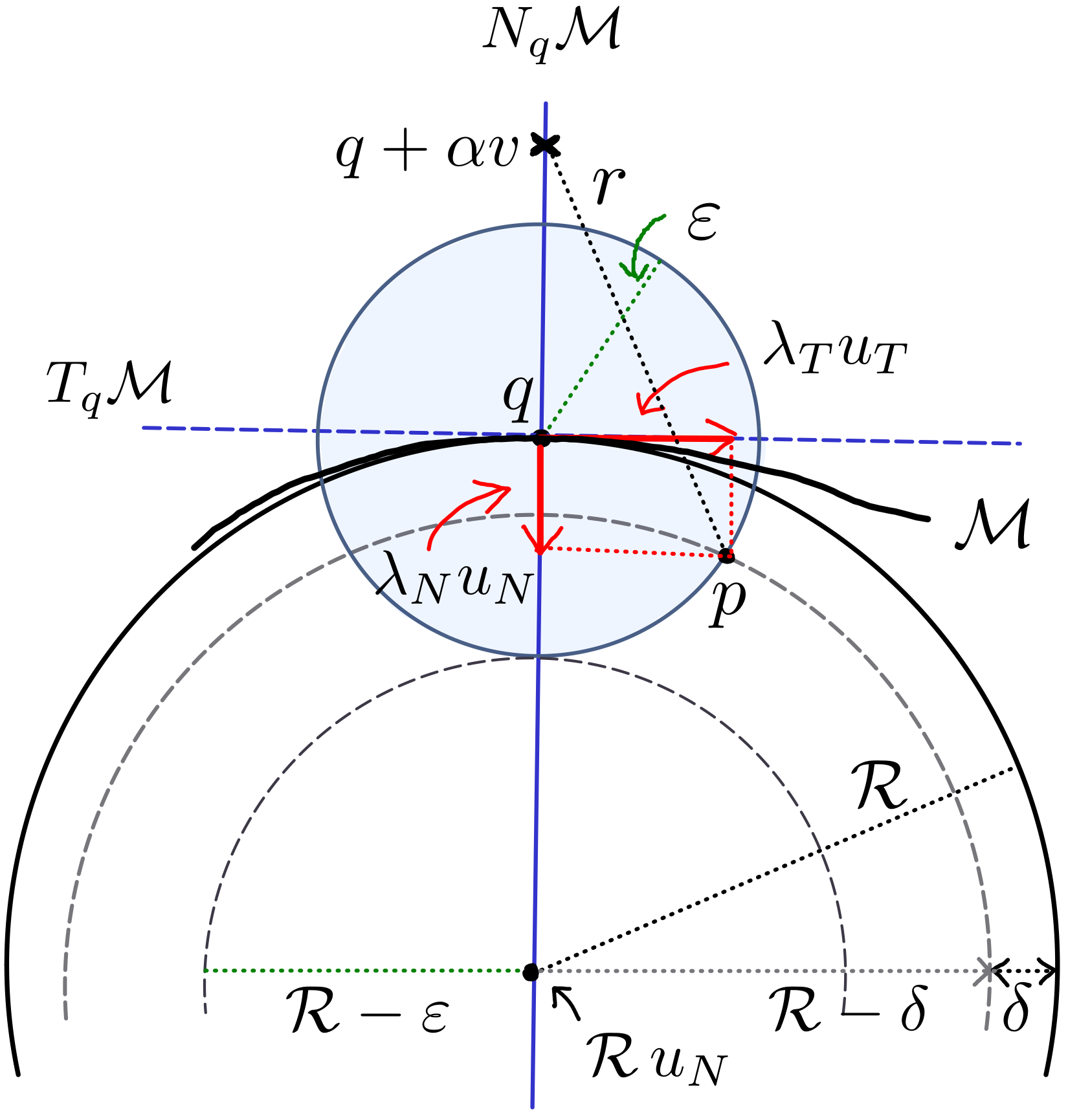
Figure 10: Overview of the notation used in the proof of Lemma A.12.

The vector $p-q$ decomposes uniquely as

$$p-q=\lambda_{T}u_{T}+\lambda_{N}u_{N},$$

with $u_{T}\in T_{q}\mathcal{M}$, $u_{N}\in N_{q}\mathcal{M}$, $\|u_{T}\|=\|u_{N}\|=1$, and $\lambda_{T},\lambda_{N}\geq 0$ (see Figure 10).

Since $\|p-q\|\leq\varepsilon$,

$$\lambda_{T}^{2}+\lambda_{N}^{2}\leq\varepsilon^{2}.$$ (14)

Thanks to [41, Theorem 4.8 (12)] (Theorem A.5), the sets $\mathcal{M}$ and
$B(q+\mathcal{R}\cdot u_{N},\mathcal{R})^{\circ}$ do not intersect, and thus:

$$p\notin B(q+\mathcal{R}\cdot u_{N},\mathcal{R}-\delta)^{\circ}.$$

Hence, $(p-q-\mathcal{R}\cdot u_{N})^{2}\geq(\mathcal{R}-\delta)^{2}$. Applying the decomposition of $p-q$ we obtain

$$\left(\lambda_{T}u_{T}+(\lambda_{N}-\mathcal{R})u_{N}\right)^{2}\geq(\mathcal{R}-\delta)^{2},$$

which implies that

$$\lambda_{T}^{2}+(\mathcal{R}-\lambda_{N})^{2}\geq(\mathcal{R}-\delta)^{2}.$$

Combining this result with Equation (14) implies that

$$\varepsilon^{2}-\lambda_{N}^{2}+(\mathcal{R}-\lambda_{N})^{2}\geq(\mathcal{R}-\delta)^{2},$$

which can be rewritten as

$$2\mathcal{R}\lambda_{N}\leq\mathcal{R}^{2}+\varepsilon^{2}-(\mathcal{R}-\delta)^{2}.$$ (15)

Choose a vector $v\in\mathrm{Nor}(q,\mathcal{M})$ with $\|v\|=1$, and let $\alpha\geq 0$. Then,

$$\left(p-(q+\alpha v)\right)^{2} =\left((\lambda_{N}u_{N}-\alpha v)+\lambda_{T}u_{T}\right)^{2}$$

$$=\left(\lambda_{N}u_{N}-\alpha v\right)^{2}+\left(\lambda_{T}u_{T}\right)^{2}$$

$$\leq(\lambda_{N}+\alpha)^{2}+\lambda_{T}^{2}$$

$$\leq(\lambda_{N}+\alpha)^{2}+\varepsilon^{2}-\lambda_{N}^{2}$$ (by (14))

$$=\alpha^{2}+2\alpha\lambda_{N}+\varepsilon^{2}.$$

Using inequality (15) to substitute $2\lambda_{N}$, we further obtain:

$$\left(p-(q+\alpha v)\right)^{2}\leq\alpha^{2}+\frac{\alpha}{\mathcal{R}}\left(\mathcal{R}^{2}+\varepsilon^{2}-(\mathcal{R}-\delta)^{2}\right)+\varepsilon^{2}.$$

Thus, if

$$r^{2}\geq\alpha^{2}+\frac{\alpha}{\mathcal{R}}\left(\mathcal{R}^{2}+\varepsilon^{2}-(\mathcal{R}-\delta)^{2}\right)+\varepsilon^{2},$$

then the point $q+\alpha v$ lies in $B(p,r)\subseteq P^{\boxplus r}$. Since this inclusion holds for any $q\in\mathcal{M}$ and $v\in N_{q}\mathcal{M}$ with $\|v\|=1$, $\mathcal{M}^{\boxplus\alpha}\subseteq P^{\boxplus r}$.

As in Proposition 4.4, we now derive a bound on $\varepsilon$. See 4.5 The bound is illustrated in Figure 2.

Proof A.14.

We combine the bound from Lemma A.12 with the conditions of Theorem 4.1. More precisely, combining Equations (2) and (13) yields the following sufficient condition for $L\cap\left(P^{\boxplus r}\right)$ to be connected:

$${\alpha^{2}+\frac{\alpha}{\mathcal{R}}\left(\mathcal{R}^{2}+\varepsilon^{2}-(\mathcal{R}-\delta)^{2}\right)+\varepsilon^{2}\leq\,r^{2}\leq\,(\mathcal{R}-\delta)^{2}-(\mathcal{R}-\alpha)^{2}.}$$ (16)

The inequality between leftmost and rightmost members of (16), which needs to be satisfied for a non-empty range of values for $r$ to exist, can be rearranged as:

$$0\geq\varepsilon^{2}-\left(\mathcal{R}-\delta\right)^{2}+\mathcal{R}^{2}+\alpha\,\frac{1}{\mathcal{R}}\left(\varepsilon^{2}-\mathcal{R}^{2}-\left(\mathcal{R}-\delta\right)^{2}\right)+2\alpha^{2}.$$

Using the abc-formula for quadratic equations, the above inequality is satisfied if $\alpha\in\left[\alpha_{\min},\alpha_{\max}\right]$, with

$$\alpha_{\min}=\frac{1}{4}\left(\frac{(\mathcal{R}-\delta)^{2}+\mathcal{R}^{2}-\varepsilon^{2}}{\mathcal{R}}-\sqrt{\Delta}\right),\alpha_{\max}=\frac{1}{4}\left(\frac{(\mathcal{R}-\delta)^{2}+\mathcal{R}^{2}-\varepsilon^{2}}{\mathcal{R}}+\sqrt{\Delta}\right),$$ (17)

where the discriminant $\Delta$ is

$$\Delta=\frac{1}{\mathcal{R}^{2}}\left(\varepsilon^{2}-\left(\mathcal{R}-\delta\right)^{2}\right)^{2}-10\left(\varepsilon^{2}-\left(\mathcal{R}-\delta\right)^{2}\right)-7\mathcal{R}^{2}.$$

The discriminant can be viewed as a polynomial in $y=\varepsilon^{2}-\left(\mathcal{R}-\delta\right)^{2}$. Solving $\Delta(y)=0$ with respect to $y$ yields $y=\mathcal{R}^{2}\left(5\pm 4\sqrt{2}\right)$. This in turn implies that $\Delta$ is non-negative if either $\varepsilon^{2}-\left(\mathcal{R}-\delta\right)^{2}\leq\mathcal{R}^{2}\left(5-4\sqrt{2}\right)$ or $\varepsilon^{2}-\left(\mathcal{R}-\delta\right)^{2}\geq\mathcal{R}^{2}\left(5+4\sqrt{2}\right)$. Thanks to Assumption 4.1, we are only interested in the case where $\varepsilon,\delta<\mathcal{R}$, and thus we can ignore the second inequality. Hence the interval $\left[\alpha_{\min},\alpha_{\max}\right]$ is non-empty if

$$\varepsilon^{2}-\left(\mathcal{R}-\delta\right)^{2}\leq\left(5-4\sqrt{2}\right)\mathcal{R}^{2}.$$

Substituting the bounds on $\alpha$ (Equation (17)) into Equations (2) and (13) yields

$$\left(1+\frac{\alpha_{\min}}{\mathcal{R}}\right)\varepsilon^{2}+\alpha_{\min}^{2}+\frac{\alpha_{\min}}{\mathcal{R}}\left(\mathcal{R}^{2}-(\mathcal{R}-\delta)^{2}\right)\leq r^{2} \leq(\mathcal{R}-\delta)^{2}-(\mathcal{R}-\alpha_{\max})^{2}.$$ (18)

Remark A.15.

We restricted ourselves to the case where $\delta\leq\varepsilon$, because if $\delta>\varepsilon$, the fact that the set of positive reach is a manifold no longer helps. The geometric reason for this is that $p$ in Figure 10 may lie in $N_{q}\mathcal{M}$.

A.3 Tightness of the bounds on the sampling parameters

In this section we prove that the bounds provided in Section A.2 are optimal in the following sense:

See 4.6

See 4.7

To prove Propositions 4.6 and 4.7, we construct the set ${\mathcal{S}}$, the manifold $\mathcal{M}$, and the corresponding samples in Examples A.19 and A.23, respectively. Due to rescaling it suffices to construct sets of reach $\mathrm{rch}({\mathcal{S}})=\mathcal{R}=1$.

Remark A.16.

The dimension of the set in both examples will be two-dimensional. As mentioned in the introduction, we expect that better bounds than (3) and (5) can be obtained for one-dimensional sets, i.e., curves, possibly with boundary.

Remark A.17.

When $\delta\geq\varepsilon$, which in Figure 2 corresponds to the area above the diagonal $\delta=\varepsilon$, the same bound is optimal whether the set is assumed to be a manifold or not. Indeed, in this case the union of annuli ${\mathcal{S}}$ in Example A.19 can be replaced by a union of circles, namely the inner boundaries of the annuli. Thus, the bound is tight for manifolds, including one-dimensional submanifolds in $\mathbb{R}^{2}$.

Remark A.18.

To simplify the analysis the samples $P$ in our examples are continuous and therefore have an infinite number of points. However these samples can be approximated arbitrarily well by finite sets because they are compact.

• Sketch of proof of Remark A.18  To pass to a finite sample, we first note that failing the bounds on the sampling parameters (in Propositions 5.2, 5.3, 6.4 and 6.5) is an open condition, i.e. for every $(\varepsilon,\delta)$ we can find an $(\varepsilon^{\prime},\delta)$ with $\varepsilon^{\prime}<\varepsilon$ such that $(\varepsilon^{\prime},\delta)$ still fail the bounds. To construct an example for a given $(\varepsilon,\delta)$ we take the example (Example A.19, A.23, B.18, and B.22 respectively) for $(\varepsilon^{\prime},\delta)$ and take a subsample of $P$ that is so dense that the one-sided Hausdorff distance is $\varepsilon$. Using the notation introduced in the Examples A.19, A.23, B.18, and B.22 we can give a more precise description of the finite sample. For sets of positive reach the finite subsample can be chosen as follows: The circle $C_{i}$ should be densely subsampled such that the subsample contains $q_{i}$. The points $p_{i}$ and $\tilde{p}_{i}$ can remain as is. For the manifolds the finite subsample of can be chosen as follows: The trimmed torus $C_{i}$ should be densely subsampled such that the subsample contains $q_{i}$ and $\tilde{q}_{i}$. Also in this context, the points $p_{i}$ and $\tilde{p}_{i}$ can remain as is. Because the samples contain $p_{i}$ and $\tilde{p}_{i}$ and $q_{i}$ ($q_{i}$ and $\tilde{q}_{i}$ respectively) (most of) the spurious cycles we examined in the Examples A.19, A.23, B.18, and B.22 remain the same. The only change that may occur for large $r$ in the proof of Proposition 5.5 is that for the interval $r\in[r_{i-1},r_{i})$ spurious $2$-cycles may be interchanged for spurious $1$-cycles. Of course for small $r$ there are many more connected components and cycles because of the discrete approximation than in the continuous examples. With these finite subsamples $P$ one still finds that the homology of $P^{\boxplus r}$ is never the same as the underlying space.  $\square$

A.3.1 Sets of positive reach

The construction of the set proving Proposition 4.6 goes as follows.

Example A.19.

We define ${\mathcal{S}}$ to be a union of annuli $A_{i}$ in $\mathbb{R}^{2}$, each of which has inner radius $1$ and outer radius $1+2\varepsilon$. We lay the annuli in a row at distance at least 2 away from each other. Due to this assumption, the reach of the set ${\mathcal{S}}$ equals 1. We number the annuli from $i=0$. Later we will see that the number of annuli that we need for the construction is finite.

The sample $P$ consists of circles $C_{i}$ of radius $1+\varepsilon$ lying in the middle of the annuli ($C_{i}\subseteq A_{i}$), and pairs of points $\{p_{i},\tilde{p}_{i}\}$. Each pair $\{p_{i},\tilde{p}_{i}\}$ lies in the disk inside the annulus $A_{i}$, at a distance $\delta$ from $A_{i}$, and the two points lie at a distance $2r_{i}$ from each other; see Figure 11, left. The bisector of $p_{i}$ and $\tilde{p}_{i}$ intersects the circle $C_{i}$ in two points. We let $q_{i}$ be the intersection point that is closest to $p_{i}$ (and thus $\tilde{p}_{i}$). We denote the circumradius of $p_{i}\tilde{p}_{i}q_{i}$ by $R_{i}$ and note that $R_{i}\geq r_{i}$. Before explaining how we pick the sequence of $r_{i}$, we state a lemma which is key for the construction:

Lemma A.20.

If $\varepsilon$ and $\delta$ fail to satisfy bound (3), that is, $\varepsilon+\sqrt{2}\,\delta>(\sqrt{2}-1),$ then

• the triangle $p_{i}\tilde{p}_{i}q_{i}$ is strictly acute;

• there exists a constant $c>0$, depending only on $\delta$ and $\varepsilon$, such that $R_{i}-r_{i}\geq c\,r_{i}$.

Proof A.21.

The situation is illustrated in Figure 11, right. Let $z_{i}$ be the centre of $C_{i}$ and let $C^{\prime}_{i}$ be the circle centred at $z_{i}$ with radius $1-\delta$. By construction, $C_{i}^{\prime}$ passes through $p_{i}$ and $\tilde{p}_{i}$, while $C_{i}$ passes through $q_{i}$. Without loss of generality, we may assume that $p_{i}$ and $\tilde{p}_{i}$ lie on a vertical line, with $p_{i}$ above the segment $z_{i}q_{i}$ and $\tilde{p_{i}}$ below it. Since $p_{i}\tilde{p}_{i}q_{i}$ is an isosceles triangle, it is acute if $\angle z_{i}q_{i}p_{i}<\frac{\pi}{4}$. The angle $\angle z_{i}q_{i}p_{i}$ is maximized when $p_{i}$ reaches the position $p^{*}_{i}$ on $C^{\prime}_{i}$ — in this position, the line through $q_{i}$ and $p_{i}$ is tangent to the circle $C^{\prime}_{i}$. Using Condition (3), we obtain that

$$\sin\angle z_{i}q_{i}p_{i}\leq\sin\angle z_{i}q_{i}p^{*}_{i}=\frac{1-\delta}{1+\varepsilon}<\frac{1}{\sqrt{2}}=\sin\frac{\pi}{4}.$$

Thus, $\angle z_{i}q_{i}p_{i}<\frac{\pi}{4}$ and therefore $p_{i}\tilde{p}_{i}q_{i}$ is acute. Because of the strict inequality in the above equation, we can find a small angle, say $\varphi=2\left(\frac{\pi}{4}-\arcsin\frac{1-\delta}{1+\varepsilon}\right)>0$, such that $\angle z_{i}q_{i}p_{i}\leq\frac{\pi}{4}-\frac{\varphi}{2}$. Since $R_{i}=\frac{r_{i}}{\sin\angle p_{i}q_{i}\tilde{p}_{i}}$, we deduce that

$$R_{i}-r_{i}=\left(\frac{1}{\sin\angle p_{i}q_{i}\tilde{p}_{i}}-1\right)r_{i}\geq\left(\frac{1}{\cos\varphi}-1\right)r_{i},$$

which, after setting $c=\frac{1}{\cos\varphi}-1$, proves the second item of the lemma.

Figure 11: Left: Each annulus $A_{i}$ is sampled by a circle $C_{i}$ and a pair of points $\{p_{i},\tilde{p}_{i}\}$. Right: Notation for the proof of Lemma A.20. If Condition (3) fails, then $\sin\angle z_{i}q_{i}p_{i}\leq\sin\angle z_{i}q_{i}p_{i}^{*}=\frac{1-\delta}{1+\varepsilon}<\frac{1}{\sqrt{2}}=\sin\frac{\pi}{4}$, and triangle $p_{i}\tilde{p}_{i}q_{i}$ is guaranteed to be acute.

We are now ready to define the distance between each pair of points $p_{i}$ and $\tilde{p}_{i}$ in an inductive manner. We set $r_{0}=\frac{\delta+\varepsilon}{2}$ and, for $i\geq 0$,

$$r_{i+1}=\begin{cases}R_{i},&\text{if }R_{i}<1-\delta,\\ 1-\delta,&\text{otherwise}.\end{cases}$$

We stop the sequence at the first value of $i$ such that $r_{i}=1-\delta$.

Assume that $\varepsilon$ and $\delta$ fail to satisfy bound (3). By Lemma A.20, $r_{i+1}-r_{i}$ is lower bounded by a positive constant that only depends on $\delta$ and $\varepsilon$,

$$r_{i+1}-r_{i}=R_{i}-r_{i}\geq c\,r_{i}\geq c\,r_{0}.$$

Hence, the sequence of $r_{i}$ reaches the value $1-\delta$ in a finite number of steps. Let $k$ be the index at which $r_{k}=1-\delta$. Our constructed set ${\mathcal{S}}$ consists of the finitely many annuli $A_{0}\cup A_{1}\cup\ldots\cup A_{k}$ and our sample $P$ is defined as $\bigcup_{0\leq i\leq k}C_{i}\cup\{p_{i},\tilde{p}_{i}\}$.

(a) For all $r<r_{0}$, the union of balls $(C_{i}\cup\{p_{i},\tilde{p}_{i}\})^{\boxplus r}$ has three connected components.

(b) At radius $r_{1}$, the cycle in the union of balls $(C_{0}\cup\{p_{0},\tilde{p}_{0}\})^{\boxplus r}$ at the annulus $A_{0}$ dies, while a cycle is created in the union of balls $(C_{1}\cup\{p_{1},\tilde{p}_{1}\})^{\boxplus r}$ at the annulus $A_{1}$.

(c) At radius $r_{2}$, the cycle in the union of balls at the annulus $A_{1}$ dies, while a cycle is created in the union of balls at the annulus $A_{2}$.

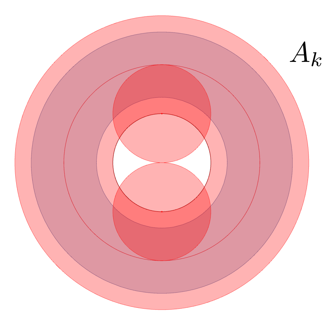
(d) The set $(C_{k}\cup\{p_{k},\tilde{p}_{k}\})^{\boxplus r}$ at radius $r_{k}=1-\delta$. The two ‘gaps’ are identical.

(e) The two ‘gaps’ of the set $(C_{k}\cup\{p_{k},\tilde{p}_{k}\})^{\boxplus r}$disappear simultaneously.

Figure 12: The changing homology of the set $P^{\boxplus r}$ in the annuli $A_{0},A_{1},A_{2}$, and $A_{k}$. The set ${\mathcal{S}}=A_{0}\cup\dots A_{k}$ is coloured light blue, the union of balls $P^{\boxplus r}$ in pink. In black we depict the circles of radius $1-\delta$.

Proof A.22 (Proof of Proposition 4.6).

We show that for any $r\geq 0$, the union of balls $P^{\boxplus r}$ has different homotopy — and even different homology — than the set ${\mathcal{S}}$. We first describe the development of the homotopy of the sets $(C_{i}\cup\{p_{i},\tilde{p}_{i}\})^{\boxplus r}$ as $r$ increases:

• For $r\in[0,r_{0})$, each set $(C_{i}\cup\{p_{i},\tilde{p}_{i}\})^{\boxplus r}$ has three connected components, as illustrated in Figure 12. The three components merge into one at $r=r_{0}$, as the two balls $\{p_{i}\}^{\boxplus r}$ and $\{\tilde{p}_{i}\}^{\boxplus r}$intersect the set $C_{i}^{\boxplus r}$.

• For $r\in[r_{i},r_{i+1})$, the set $(C_{i}\cup\{p_{i},\tilde{p}_{i}\})^{\boxplus r}$ has the homotopy type of two circles that share a point (also known as a wedge of two circles or a bouquet), as illustrated in Figures 12 and 12. The smaller ‘gap’ creating the additional cycle appears when $r=r_{i}$. Since, due to Lemma A.20, the triangle $p_{i}\tilde{p}_{i}q_{i}$ is acute, the ‘gap’ persists until $r=R_{i}=r_{i+1}$. All sets $(C_{j}\cup\{p_{j},\tilde{p}_{j}\})^{\boxplus r}$ with $j\neq i$ have the homotopy type of a circle.

• At $r=r_{k}=1-\delta$, all sets $(C_{i}\cup\{p_{i},\tilde{p}_{i}\})^{\boxplus r}$ have the homotopy type of a circle but the last one, $(C_{k}\cup\{p_{k},\tilde{p}_{k}\})^{\boxplus r}$, which has the homotopy type of two circles that share a point (see Figure 12). Unlike the other cases, however, the ‘gaps’ in the set $(C_{k}\cup\{p_{k},\tilde{p}_{k}\})^{\boxplus r}$ are identical, and disappear simultaneously at $r=R_{k}\left(=\tfrac{(1+\varepsilon)^{2}+(1-\delta)^{2}}{2(1+\varepsilon)}\right)$ (Figure 12). For larger $r$, the set $(C_{k}\cup\{p_{k},\tilde{p}_{k}\})^{\boxplus r}$ is contractible.

Each annulus $A_{i}\subseteq{\mathcal{S}}$ has the homotopy type of a circle, and thus the dimensions of the homologies of the set ${\mathcal{S}}$ equal

$$\dim\left(H_{0}({\mathcal{S}})\right)=k+1,\qquad\dim\left(H_{1}({\mathcal{S}})\right)=k+1.$$

The dimensions of the homologies of the set $P^{\boxplus r}$ are recorded in the table below.

tabular|c || c | c |c|   $r\in[0,r_{0})$ $r\in\left[r_{0},R_{k}\right)$ $r\geq R_{k}$

$\dim\left(H_{0}\left(P^{\boxplus r}\right)\right)$ $3(k+1)$ $k+1$ $\leq k+1$

$\dim\left(H_{1}\left(P^{\boxplus r}\right)\right)$ $k+1$ $k+2$ $\leq k$

One sees that the set ${\mathcal{S}}$ never has the same homology as the union of balls $P^{\boxplus r}$, and thus the two never have the same homotopy.

A.3.2 Manifolds

The construction of the manifold proving Proposition 4.7 goes as follows:

Example A.23.

We define $\mathcal{M}$ to be a union of tori of revolution $T_{i}$ in $\mathbb{R}^{3}$. Each of these tori is the $1$-offset of a circle of radius $2$ in $\mathbb{R}^{3}$. Put differently, each $T_{i}$ is — up to Euclidean transformations — the surface of revolution of a circle of radius $1$ in the $xz$-plane, centred at $(2,0,0)$, around the $z$-axis. The set $T_{i}$ is illustrated in blue in Figures 13 and 14.

We number the tori from $i=0$, and lay them out in a row at a distance at least $2$ apart from one another. Due to this assumption, the reach of $\mathcal{M}$ equals 1. Later we will see that the number of tori that we need for the construction is finite.

The sample $P$ consists of sets $C_{i}$ which are tori with a part cut out, and pairs of points $\{p_{i},\tilde{p}_{i}\}$ lying inside the hole of each torus $T_{i}$. To construct each set $C_{i}$ we take the $\delta$-offset of $T_{i}$, keep the part that lies inside the solid torus bounded by $T_{i}$, and remove an $\varepsilon$-neighbourhood of the circle obtained by revolving the point $(1,0,0)$ around the $z$-axis; see the red set in Figures 13 and 14. In other words, each $C_{i}$ is the set difference between the torus obtained by rotating the circle of radius $1-\delta$ centred in the $xz$-plane at $(2,0,0)$, and the open solid torus obtained by rotating the open disc of radius $\varepsilon$ centred in the $xz$-plane at $(1,0,0)$.

Figure 13: The (half of the) torus $T_{i}$ depicted in blue; the sample — the set $C_{i}$ and the points $p_{i}$ and $\tilde{p}_{i}$ — in red. In black we indicate the circle $C^{\prime}_{i}$. The closest point projection of this circle onto $\mathcal{M}$ is indicated in blue.

Let $C^{\prime}_{i}$ be the circle found by revolving the point $(1-\delta,0,0)$ around the $z$-axis. Each pair of points, $p_{i}$ and $\tilde{p}_{i}$, lies on $C^{\prime}_{i}$ at a distance $2r_{i}$ from each other. Let $q_{i}$ and $\tilde{q}_{i}$ be the two points in the intersection of the bisector of $p_{i}$ and $\tilde{p}_{i}$ and the set $C_{i}$ that lie closest to $p_{i}$ and $\tilde{p}_{i}$. Note that $q_{i}$ and $\tilde{q}_{i}$ lie on the boundary of $C_{i}$, and $\{q_{i},\tilde{q}_{i}\}=\pi_{C_{i}}\left(\frac{p_{i}+\tilde{p}_{i}}{2}\right)$. Denote the circumradius of the simplex $p_{i}\tilde{p}_{i}q_{i}\tilde{q}_{i}$ by $R_{i}$.

Figure 14: The sets $T_{i}$, $C_{i}$ and $C^{\prime}_{i}$ are obtained by rotating around the $z$-axis, respectively, the blue circles, the red arcs and the white point.

As in Example A.19, we define the distance $2r_{i}$ between each pair of points $p_{i}$ and $\tilde{p}_{i}$ inductively. We set the distance $r_{0}$ such that the balls $B(p_{0},r)$ and $B(\tilde{p}_{0},r)$ start to intersect each other at the same value of $r$ as the balls $B(q_{0},r)$ and $B(\tilde{q}_{0},r)$ start to intersect:

$$r_{0}=\tfrac{1}{2}d\left(q_{0},\tilde{q}_{0}\right).$$

We then define

$$r_{i+1}=\begin{cases}R_{i},&\text{if }R_{i}<1-\delta,\\ 1-\delta,&\text{otherwise}.\end{cases}$$

We stop the sequence at the first value of $i$ such that $r_{i}=1-\delta$.

Assume that $\varepsilon$ and $\delta$ fail to satisfy bound (5). By Lemma A.25, $r_{i+1}$ is lower bounded by a positive constant that only depends on $\delta$ and $\varepsilon$,

$$r_{i+1}^{2}=R_{i}^{2}\geq r_{i}^{2}+c^{2}\geq r_{0}^{2}+i\cdot c^{2}.$$

Hence, the sequence of $r_{i}$ reaches the value $1-\delta$ in a finite number of steps.

Let $k$ be the index at which $r_{k}=1-\delta$. Our constructed manifold $\mathcal{M}$ consists of the finitely many tori $T_{0}\cup T_{1}\cup\ldots\cup T_{k}$, and our sample $P$ is defined as $\bigcup_{0\leq i\leq k}\left(C_{i}\cup\{p_{i},\tilde{p}_{i}\}\right)$.

In the proof of Proposition 4.6, acuteness of triangles plays an essential role. In Lemma A.20 we argue that if $\varepsilon$ and $\delta$ fail to satisfy Bound (3), then any triangle $p_{i}\tilde{p}_{i}q_{i}$ is acute. Furthermore, a triangle is acute if and only if it contains its circumcentre. We generalize acuteness to simplices as follows:

Definition A.24 (Self-centred simplices, [33]).

A simplex is called (strictly) self-centred if it contains its circumcentre (in its interior).

Lemma A.25.

If $\varepsilon$ and $\delta$ fail to satisfy bound (5), that is, $(1-\delta)^{2}-\varepsilon^{2}<4\sqrt{2}-5$, and $r_{i}$ satisfies

$$2r_{i}\geq d(q_{i},\tilde{q}_{i}),$$ (19)

then

• the simplex $p_{i}\tilde{p}_{i}q_{i}\tilde{q}_{i}$ is strictly self-centred;

• there exists a constant $c>0$, depending only on $\delta$ and $\varepsilon$, such that $R_{i}^{2}\geq r_{i}^{2}+c^{2}$.

Proof A.26.

A key observation is that the simplex $p_{i}\tilde{p}_{i}q_{i}\tilde{q}_{i}$ is (strictly) self-centred if and only if the triangles $p_{i}\tilde{p}_{i}q_{i}$ and $q_{i}\tilde{q}_{i}p_{i}$ are (strictly) acute.

To see this, assume without loss of generality that the torus $T_{i}$ is centred at the origin and that the points $q_{i}$ and $\tilde{q}_{i}$ lie in the $xz$-plane and have positive $x$-coordinates, as in Figure 14. The circumcentre of a simplex is the intersection of the bisectors of pairs of its vertices. The circumcentre of the simplex $p_{i}\tilde{p}_{i}q_{i}\tilde{q}_{i}$ thus lies on the $x$-axis; indeed, the $x$-axis is the intersection of the bisector of $p_{i}$ and $\tilde{p}_{i}$, and the bisector of $q_{i}$ and $\tilde{q}_{i}$.

Hence, $p_{i}\tilde{p}_{i}q_{i}\tilde{q}_{i}$ is strictly self-centred if and only if its circumcentre lies on the intersection of the interior of $p_{i}\tilde{p}_{i}q_{i}\tilde{q}_{i}$ with the $x$-axis — the open line segment connecting the midpoint $m_{i}=\frac{p_{i}+\tilde{p}_{i}}{2}$ of $p_{i}$ and $\tilde{p}_{i}$ with the midpoint $n_{i}=\frac{q_{i}+\tilde{q}_{i}}{2}$ of $q_{i}$ and $\tilde{q}_{i}$. This happens precisely when the circumcentre of triangle $p_{i}\tilde{p}_{i}q_{i}$ (resp. $q_{i}\tilde{q}_{i}p_{i}$) lies on the open segment connecting $m_{i}$ to $q_{i}$ (resp. $n_{i}$ to $p_{i}$), in other words, when both triangles $p_{i}\tilde{p}_{i}q_{i}$ and $q_{i}\tilde{q}_{i}p_{i}$ are strictly acute. We illustrate the two extreme cases in Figure 15.

We prove the fact that the two triangles are indeed strictly acute in Claim 1 below.

Figure 15: When both triangles $p_{i}\tilde{p}_{i}q_{i}$ and $q_{i}\tilde{q}_{i}p_{i}$ are strictly acute, the circumcentre $Z_{i}$ of tetrahedron $p_{i}\tilde{p}_{i}q_{i}\tilde{q}_{i}$ lies on the open segment connecting $m_{i}$ to $n_{i}$. When the triangle $p_{i}\tilde{p}_{i}q_{i}$ becomes right-angled, $Z_{i}$ reaches $m_{i}$ (on the left). When the triangle $q_{i}\tilde{q}_{i}p_{i}$ becomes right-angled, $Z_{i}$ reaches $n_{i}$ (on the right).

Recall that both the circumcentre of the simplex $p_{i}\tilde{p}_{i}q_{i}\tilde{q}_{i}$ and the point $m_{i}$ lie on the $x$-axis. Let $u$ be the $x$-coordinate of the circumcentre. We have shown that, for all distances $r_{i}\in\left[\tfrac{1}{2}d(q_{i},\tilde{q}_{i}),1-\delta\right]$ defining the position of the points $p_{i}$ and $\tilde{p}_{i}$, the circumcentre lies further away from the origin than the midpoint $m_{i}$. That is, $u-\left\|{m_{i}}\right\|>0$. Since $\left[\tfrac{1}{2}d(q_{i},\tilde{q}_{i}),1-\delta\right]$ is compact, there exists a constant $c$ such that

$$u-\left\|{m_{i}}\right\|\geq c.$$

The triangle with vertices $p_{i},m_{i}$, and the circumcentre is right-angled, with edge lengths $r_{i},u-\left\|{m_{i}}\right\|$, and the hypotenuse $R_{i}$. Thus,

$$R_{i}^{2}=r_{i}^{2}+{(u-\left\|{m_{i}}\right\|)}^{2}\geq r_{i}^{2}+c^{2}.$$

Claim 1.

The triangles $p_{i}\tilde{p}_{i}q_{i}$ and $q_{i}\tilde{q}_{i}p_{i}$ are strictly acute, under the assumptions of Lemma A.25.

Proof A.27.

Figure 16: Zoom-in of Figure 14 with the notation used in the proof of Claim 1.

Let $t\geq 0$ be the $x$-coordinate of $p_{i}$, and $\ell$ and $h$ define the $x$- and $z$-coordinates of $q_{i}$,

$$p_{i}=(t,r_{i},0),\qquad{q_{i}=(1+\ell,0,h)}.$$

Then $m_{i}=(t,0,0)$ and $n_{i}=(1+\ell,0,0)$. We refer the reader to Figure 16 for an overview of the notation.

Due to the Pythagorean theorem,

$$\varepsilon^{2}-\ell^{2}=h^{2}=(1-\delta)^{2}-(1-\ell)^{2},$$

and thus

$$\ell=\frac{\varepsilon^{2}-\delta^{2}+2\delta}{2}\quad\text{and}\quad h=\sqrt{\varepsilon^{2}-\ell^{2}}.$$

Furthermore, due to Equation (19),

$$r_{i}\geq\tfrac{1}{2}d(q_{i},\tilde{q}_{i})=h.$$

Note that the positions of both points $p_{i}$ and $\tilde{p}_{i}$ on the circle $C_{i}^{\prime}$ are completely determined by $r_{i}$ (the $y$-coordinate of $p_{i}$). For the purpose of the proof, we use the $x$-coordinate $t=\sqrt{(1-\delta)^{2}-r_{i}^{2}}$ of $p_{i}$ to parametrize the positions of $p_{i}$ and $\tilde{p}_{i}$. Hence, showing that triangles $p_{i}\tilde{p}_{i}q_{i}$ and $q_{i}\tilde{q}_{i}p_{i}$ are acute for all $r_{i}\in[h,1-\delta]$ translates into showing that they are acute for all $0\leq t\leq\sqrt{(1-\delta)^{2}-h^{2}}=1-\ell$.

The triangle $p_{i}\tilde{p}_{i}q_{i}$ is isosceles. It is thus strictly acute if and only if its height, $\left\|{m_{i}-q_{i}}\right\|$, is larger than half the length of its base, $\left\|{m_{i}-p_{i}}\right\|=r_{i}$. We obtain:

$$r_{i}^{2}<\left\|{m_{i}-q_{i}}\right\|^{2}$$

$$\iff (1-\delta)^{2}-t^{2}<(1+\ell-t)^{2}+h^{2}$$

$$\iff 0<2t^{2}-2t(1+\ell)+4\ell.$$ (20)

Let $Q(t)=2t^{2}-2t(1+\ell)+4\ell$ be the quadratic form from the inequality (A.27), and $\Delta$ be its reduced discriminant,

$$\Delta=(1+\ell)^{2}-8\ell=(\ell-3-2\sqrt{2})(\ell-3+2\sqrt{2}).$$

The inequality (A.27) holds for all $t\in\left[0,1-\ell\right]$ if and only if

• either $\Delta<0$, and thus $Q(t)>0$ for all $t$, or

• $\Delta\geq 0$ and the interval $[t_{1},t_{2}]\ni t$ for which $Q(t)\leq 0$, is disjoint from the interval $\left[0,1-\ell\right]$.

$\Delta<0$ if and only if $3-2\sqrt{2}<\ell<3+2\sqrt{2}$. Substituting $2\ell=\varepsilon^{2}-(1-\delta)^{2}+1$ translates into

$$5-4\sqrt{2}<\varepsilon^{2}-(1-\delta)^{2}<5+4\sqrt{2}.$$

The first inequality holds by assumption. The second follows from the fact that $0\leq\delta\leq\varepsilon<1$.

In summary, our assumptions imply that $\Delta<0$, implying that $Q>0$, and thus the triangle $p_{i}\tilde{p}_{i}q_{i}$ is strictly acute.

Similarly, the triangle $q_{i}\tilde{q}_{i}p_{i}$ is isosceles, and is thus strictly acute if and only if its height, $\left\|{n_{i}-p_{i}}\right\|$, is larger than half the length of its base, $\left\|{n_{i}-q_{i}}\right\|=h$. This indeed holds, since

$$\left\|{n_{i}-p_{i}}\right\|^{2}=(1+\ell-t)^{2}+r_{i}^{2}\geq(1+\ell-t)^{2}+h^{2}>h^{2}.$$

Proof A.28 (Proof of Proposition 4.7).

We show that for any $r\geq 0$, the union of balls $P^{\boxplus r}$ has different homotopy than the manifold $\mathcal{M}$. To achieve this, it suffices to show that their homologies differ.

The manifold $\mathcal{M}$ consists of $k+1$ tori, and thus the dimensions of the homologies of $\mathcal{M}$ equal

$$\dim\left(H_{0}(\mathcal{M})\right)=k+1,\qquad\dim\left(H_{1}(\mathcal{M})\right)=2(k+1),\qquad\dim\left(H_{2}(\mathcal{M})\right)=k+1.$$

We first have a look at the second homology of the set $(C_{i}\cup\{p_{i},\tilde{p}_{i}\})^{\boxplus r}$. For $r<r_{0}$, as well as $r\geq 1-\delta$, the second homology of the set $(C_{i}\cup\{p_{i},\tilde{p}_{i}\})^{\boxplus r}$ is trivial for each $i$. In the former case (see Figure 18), the set $(C_{i})^{\boxplus r}$ has not yet ‘closed up’ to form a (thickened) torus. In the latter case, the inside of the torus $(C_{i})^{\boxplus r}$ gets filled in. Thus,

$$\dim\left(H_{2}\left(P^{\boxplus r}\right)\right) =0 r\in[0,r_{0})\cup[1-\delta,\infty).$$ for

In contrast, $\dim\left(H_{2}(\mathcal{M})\right)=k+1$. Thus, $\mathcal{M}$ and $P^{\boxplus r}$ have different homology for $r\in[0,r_{0})\cup[1-\delta,\infty)$.

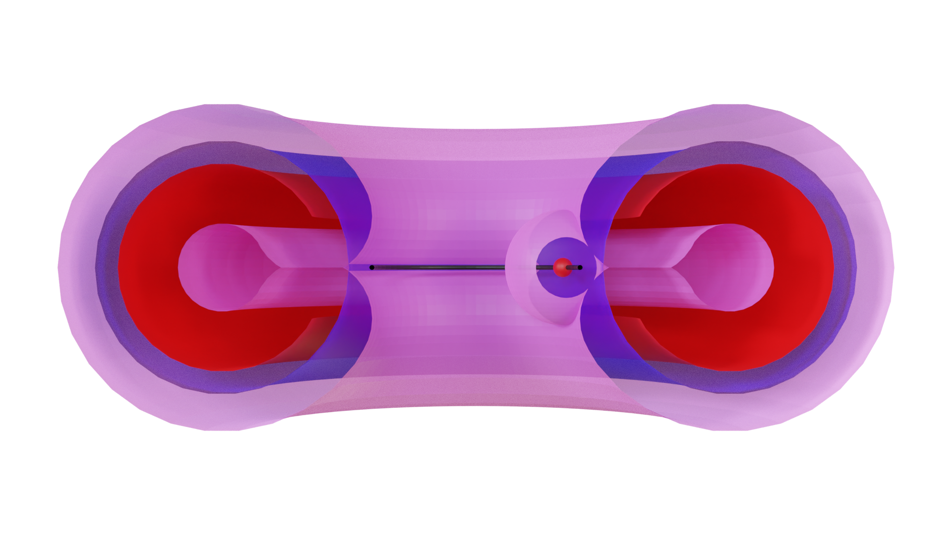
Figure 17: The spurious 2-cycle that prevents the sample from having the same homology as the manifold. The manifold $\mathcal{M}$ is depicted in blue, the sample $P$ in red, and the boundary of the thickening in pink. The cycle is clearly present in the zoomed-in image (bottom).

Figure 18: Two views of the situation at $r_{0}$. The sample $P$ in red and its thickening $P^{\boxplus r_{0}}$ in purple. The balls $B(p_{0},r_{0})$ and $B(\tilde{p}_{0},r_{0})$ touch precisely and the thickened torus $(C_{0})^{\boxplus r_{0}}$ ‘closes up’ and generates 2-homology.

For $r\in[r_{i-1},r_{i})$, the set $(C_{i}\cup\{p_{i},\tilde{p}_{i}\})^{\boxplus r}$ has the homotopy type of a torus with either at least a circle or a single 2-sphere attached,depending on whether the radius $r$ is smaller or larger than the circumradius of the triangle $p_{i}\tilde{p}_{i}q_{i}$. The smaller ‘gap’ creating the additional 1-, and later 2-cycle appears when $r=r_{i}$. Since, due to Lemma A.25, the simplex $p_{i}\tilde{p}_{i}q_{i}\tilde{q}_{i}$ is self-centred, the gap persists until $r=R_{i}=r_{i+1}$.

All sets $(C_{j}\cup\{p_{j},\tilde{p}_{j}\})^{\boxplus r}$ with $j\neq i$ have the homotopy type of a torus. Thus, for $r\in[r_{0},1-\delta)$,

$$\dim\left(H_{1}\left(P^{\boxplus r}\right)\right)+\dim\left(H_{2}\left(P^{\boxplus r}\right)\right)=3(k+1)+1.$$

In contrast, $\dim\left(H_{1}(\mathcal{M})\right)+\dim\left(H_{2}(\mathcal{M})\right)=3(k+1),$ and thus the manifold $\mathcal{M}$ and the union of balls $P^{\boxplus r}$ have different homology also for $r\in[r_{0},1-\delta)$.

(a) At first, the balls around the points $p_{i}$ and $\tilde{p}_{i}$ do not intersect the thickening of the set $C_{i}$, and thus the number of connected components of the thickening (in pink) of $P$ is different from the number of components of the manifold.

(b) Then we create a (or possibly multiple) spurious cycle(s) for the first torus in the sequence (on the left).

(c) By the time the spurious cycles at the first torus have disappeared, others have been created at the second torus. This process is then repeated for all tori in the sequence as $r$ increases.

(d) The points $p_{k}$ and $\tilde{p}_{k}$ lie in the symmetry plane for the final torus $T_{k}$ in the row of tori.

Figure 19: The construction for manifolds imitates the construction for general sets of positive reach as much as possible. The manifold $\mathcal{M}$ is depicted in blue, the sample $P$ in red, and the thickening in pink. We only display the part of objects below a horizontal clipping plane.

Appendix B Subsets of Riemannian manifolds

In this section we extend our analysis from the Euclidean setting to Riemannian manifolds with bounded curvature. We assume that the author is familiar with the basics of Riemannian geometry. We will be using results from comparison theory, which, for the convenience of the reader, we recall in Appendix C.

B.1 Definitions and settings

Before we can state and prove our homotopy reconstruction result, we need to generalize Federer’s notions and results (Section A.1) to Riemannian manifolds. This includes an appropriate definition of the reach, as well as a generalization of Federer’s Theorem 4.8(12) (Theorem A.5) and an extension of the normal cone.

Throughout this section we will be working with the distance function, the closest point projection, and the medial axis. To this end, let ${\mathcal{S}}$ be a closed non-empty subset of an ambient manifold $\mathcal{N}$. We denote the distance function to ${\mathcal{S}}$ by

$$\rho_{{\mathcal{S}}}:\mathcal{N}\to\mathbb{R},\qquad\rho_{{\mathcal{S}}}(q):=\inf\{d_{\mathcal{N}}(q,p)\mid p\in{\mathcal{S}}\}.$$ (21)

We write $\pi_{\mathcal{S}}(q)$ for the set of points $p\in{\mathcal{S}}$ such that $d_{\mathcal{N}}(q,p)=\rho_{{\mathcal{S}}}(q)$, and call the set $\pi_{\mathcal{S}}$ the closest point projection of $q$ onto ${\mathcal{S}}$. The medial axis of ${\mathcal{S}}$ is the set of those points in ${\mathcal{S}}$ whose closest point projection consists of more than one point:

$$\textrm{ax}_{\mathcal{N}}({\mathcal{S}}):=\{q\in\mathcal{N}\mid\operatorname{Card}(\pi_{\mathcal{S}}(q))>1\},$$ (22)

where $\operatorname{Card}(A)$ denotes the cardinality of the set $A$.

The cut locus reach.

Generalizations of the reach have been studied before; however, none of the existing definitions fit our purpose. We thus introduce a new variant of the reach that is optimal in our setting. In addition, we discuss the various definitions of the reach in Appendix F.

Our variant of the reach is based on the cut locus. The cut locus (see for example [16]) is commonly defined for a single point — say $p$ — in a Riemannian manifold, and consists of those points in the manifold, for which there is no unique geodesic to $p$.

See 5.1 Observe that the cut locus contains the medial axis, that is, $\textrm{ax}_{\mathcal{N}}({\mathcal{S}})\subseteq\operatorname{cl}_{\mathcal{N}}({\mathcal{S}})$.

See 5.2

The key tool: the flow

In [9], the authors extend the result of [57], namely that any open bounded subset of Euclidean space has the same homotopy type as its medial axis, to the more general situation of an open bounded subset $\Omega$ of a Riemannian manifold. By using some tools of non-smooth analysis, namely the properties of semi-concave functions, as well as some Riemannian geometry, they generalize the result of [57] while providing a shorter proof. However, the underlying idea in both [9] and [57] is the same, which is to use the flow: given an open bounded subset $\Omega$ of a Riemannian manifold, the flow $\Phi:\Omega\times[0,\infty)\rightarrow\Omega$ is induced by a generalized gradient of the distance function on its boundary $\partial\Omega$. It is continuous, and realizes a homotopy equivalence — more precisely, a weak deformation retraction — between the set $\Omega$ and the cut locus of its boundary $\partial\Omega$. We refer the reader to Appendix G.1 for more details.

We consider a flow given on a complement of a closed subset ${\mathcal{S}}\subseteq\mathcal{N}$:

$$\Phi_{{\mathcal{S}}}:\left(\mathcal{N}\setminus{\mathcal{S}}\right)\times[0,\infty)\rightarrow\mathcal{N}\setminus{\mathcal{S}},\qquad(p,t)\mapsto\Phi_{{\mathcal{S}}}(p,t).$$ (23)

Roughly speaking, the flow follows the steepest ascent of the distance function. The precise definition of the flow $\Phi_{{\mathcal{S}}}$ is extensive and described in detail in Appendix G.2. We refer the reader to Equation (61) for an explicit formula, and note that, thanks to Lemmas 3.4 and 3.5 as well as proof of Theorem 5.3 in [9], $\Phi_{{\mathcal{S}}}$ is locally Lipchitz in $p$ and $1$-Lipschitz in $t$.

In the next two lemmas we leverage the properties of the flow $\Phi_{{\mathcal{S}}}$ to trace minimizing geodesics and define a deformation retract onto the set ${\mathcal{S}}$. The next two lemmas show that near a set of positive cut locus reach the flow $\Phi_{{\mathcal{S}}}$ goes along geodesics, which in turn yields a generalization of part of Federer’s Theorem 4.8(12) (Theorem A.5), and that the flow induces a deformation retract on a set of positive reach. The proofs of the lemmas are given in Appendix G.2.

Lemma B.1.

Let $0<\rho<\mathrm{rch}^{\operatorname{cl}}_{\mathcal{N}}({\mathcal{S}})$. Then for any point $p\in{\mathcal{S}}^{\boxplus\rho}\setminus{\mathcal{S}}$, and any parameter $t\in\rho-\rho_{{\mathcal{S}}}(p)$, there is a unique minimizing geodesic from the point $\Phi_{{\mathcal{S}}}(p,t)$ to ${\mathcal{S}}$. Moreover,

$$\pi_{{\mathcal{S}}}(\Phi_{{\mathcal{S}}}(p,t))=\pi_{{\mathcal{S}}}(p),$$

and the minimizing geodesic from $\Phi_{{\mathcal{S}}}(p,t)$ to ${\mathcal{S}}$ is the concatenation of the minimizing geodesic from $p$ to ${\mathcal{S}}$ with the trajectory $\Phi_{{\mathcal{S}}}(p,[0,t])$.

Corollary B.2.

Let ${\mathcal{S}}\subseteq\mathcal{N}$ be a closed set. Pick a point $p\in\mathcal{N}$ satisfying $0<\rho_{{\mathcal{S}}}(p)<\mathrm{rch}^{\operatorname{cl}}_{\mathcal{N}}({\mathcal{S}})$, and define

$$\zeta:=\mathrm{rch}^{\operatorname{cl}}_{\mathcal{N}}({\mathcal{S}})-\rho_{{\mathcal{S}}}(p).$$

The domain of the flow $\Phi_{{\mathcal{S}}}$ can be extended to negative values of $t$, namely $t\in[-\rho_{{\mathcal{S}}},\,\zeta]$. We denote this extension by $\overline{\Phi_{{\mathcal{S}}}}$, and define it via the geodesic segment extending the geodesic from $p$ to $\pi_{{\mathcal{S}}}(p)$. For every point $y$ on this segment, we have $\pi_{\mathcal{S}}(y)=\pi_{\mathcal{S}}(p)$. Because the balls centered at $y$ with radius $d(y,\pi_{\mathcal{S}}(p))$ are nested, we have in particular that

$$B\left(p,\,\rho_{{\mathcal{S}}}(p)\right)^{\circ}\subseteq B\left(\Phi_{{\mathcal{S}}}(p,\zeta),\,\mathrm{rch}^{\operatorname{cl}}_{\mathcal{N}}({\mathcal{S}})\right)^{\circ}\subseteq\mathcal{N}\setminus{\mathcal{S}}.$$

The complement of the open offset of ${\mathcal{S}}$ is defined as

$$\mathsf{C}^{\rho}({\mathcal{S}}):=\left\{p\in\mathcal{N}\mid\rho_{\mathcal{S}}(p)\geq\rho\right\}.$$ (24)

Lemma B.3.

Let $0<\rho<\rho^{\prime}<\mathrm{rch}^{\operatorname{cl}}_{\mathcal{N}}({\mathcal{S}})$. Then

$$\mathrm{rch}^{\operatorname{cl}}_{\mathcal{N}}(\mathsf{C}^{\rho^{\prime}}({\mathcal{S}}))\geq\rho^{\prime},$$ (25)

and the homotopy $\mathcal{H}:{\mathcal{S}}^{\boxplus\rho}\times[0,\rho]\rightarrow{\mathcal{S}}^{\boxplus\rho}$, defined by

$$\mathcal{H}(p,t):=\begin{cases}p&\text{if}\quad p\in{\mathcal{S}},\\ \Phi_{\mathsf{C}^{\rho^{\prime}}({\mathcal{S}})}\left(p,\max(t,\rho_{{\mathcal{S}}}(p))\right)&\text{if}\quad p\notin{\mathcal{S}},\end{cases}$$ (26)

realizes a deformation retract from the thickening ${\mathcal{S}}^{\boxplus\rho}$ to the set ${\mathcal{S}}$ where the trajectory of each point is a minimizing geodesic to ${\mathcal{S}}$.

The normal cone.

Finally, we extend the normal cone and the tangent cone to the Riemannian setting, keeping for both the same notation as in the Euclidean case, that is, omitting the reference to the Riemannian manifold $\mathcal{N}$.

Definition B.4 (Normal cone).

For a point $q\in{\mathcal{S}}$, we define the normal cone to ${\mathcal{S}}$ at $q$ by

$$\mathrm{Nor}(q,{\mathcal{S}}):=\left\{\lambda v\in\mathrm{Tan}(q,\mathcal{N})\mid\lambda\geq 0\text{ and }\exists\,p\in\mathcal{N}\setminus{\mathcal{S}}\text{ with }p=\exp_{q}(v)\text{ and }|v|=\rho_{{\mathcal{S}}}(p)\right\}.$$

Remark B.5.

Note that in Definition B.4 one has $q=\pi_{{\mathcal{S}}}(p)$. Moreover, we can easily check that $\mathrm{Nor}(q,{\mathcal{S}})$ is a subset of the dual cone of the tangent cone, which can be derived from the Definition A.2 for Euclidean space as

$$\mathrm{Tan}(q,{\mathcal{S}}):=\mathrm{Tan}(0,\exp_{q}^{-1}({\mathcal{S}}\cap B(q,\rho))$$

where $\rho>0$ is smaller than the injectivity radius of $\mathcal{N}$.

The reverse inclusion holds as well but we do not need it there.

Lemma B.6.

Given a closed subset ${\mathcal{S}}\subseteq\mathcal{N}$ such that $\mathrm{rch}^{\operatorname{cl}}_{\mathcal{N}}({\mathcal{S}})>0$, a point $q\in{\mathcal{S}}$ and a vector $v\in\mathrm{Nor}(q,{\mathcal{S}})$ with $|v|=1$, then for any $\lambda<\mathrm{rch}^{\operatorname{cl}}_{\mathcal{N}}({\mathcal{S}})$, the curve $\exp_{q}([0,\lambda v])$ is the unique minimizing geodesic connecting the point $\exp_{q}(\lambda v)$ with the set ${\mathcal{S}}$.

Proof B.7.

With Definition B.4 of the normal cone $\mathrm{Nor}(q,{\mathcal{S}})$, the proof follows from Lemma B.1.

Settings.

In the Riemannian setting, we let $B(p,r)=\{x\in\mathcal{N}\mid d_{\mathcal{N}}(p,x)\leq r\}$ designate a geodesic ball of $\mathcal{N}$ and $X^{\boxplus r}=\bigcup_{x\in X}B(x,r)$ designate a union of geodesic balls. With all the necessary notions in place, we recall the setting we assume for the remainder of Section B:

B.2 The geometric argument

In this section we show that if the union of (geodesic) balls $P^{\boxplus r}=\bigcup_{p\in P}B(p,r)$ covers a sufficiently large neighbourhood of ${\mathcal{S}}$ and the parameter $r$ is not too big, $P^{\boxplus r}$ deformation-retracts to ${\mathcal{S}}$.

Theorem B.8.

Assume that a parameter $\alpha>0$ is small enough, so that the $\alpha$-neighbourhood ${\mathcal{S}}^{\boxplus\alpha}$ of the set ${\mathcal{S}}$ is contained in the union of balls $P^{\boxplus r}$. In other words,

$${\mathcal{S}}^{\boxplus\alpha}\subseteq P^{\boxplus r}.$$ (27)

Define

$$f_{\Lambda_{\ell}}(\mathcal{R},\delta,\alpha)\underset{\text{def.}}{=}\>\begin{cases}\frac{1}{\sqrt{{\Lambda_{\ell}}}}\arccos\frac{\cos\sqrt{{\Lambda_{\ell}}}\>(\mathcal{R}-\delta)}{\cos\sqrt{{\Lambda_{\ell}}}\>(\mathcal{R}-\alpha)}&\text{if}\quad{\Lambda_{\ell}}>0,\\ \sqrt{(\mathcal{R}-\delta)^{2}-(\mathcal{R}-\alpha)^{2}}&\text{if}\quad{\Lambda_{\ell}}=0,\\ \frac{1}{\sqrt{{{\left\lvert{\Lambda_{\ell}}\right\rvert}}}}\operatorname*{arccosh}\frac{\cosh\sqrt{{{\left\lvert{\Lambda_{\ell}}\right\rvert}}}\>(\mathcal{R}-\delta)}{\cosh\sqrt{{{\left\lvert{\Lambda_{\ell}}\right\rvert}}}\>(\mathcal{R}-\alpha)}&\text{if}\quad{\Lambda_{\ell}}<0.\end{cases}$$ (28)

Moreover, for any point $q\in{\mathcal{S}}$ and any vector $v\in\mathrm{Nor}(q,{\mathcal{S}})$, let $\gamma_{q,v}(t)$ be the (arc length parametrized) geodesic emanating from $q$ in the direction $v$, and write

$$L\underset{\text{def.}}{=}\>\{\gamma_{q,v}(t)\mid t\in[0,\mathcal{R})\}.$$

If

$$r<f_{\Lambda_{\ell}}(\mathcal{R},\delta,\alpha),$$ (29)

then the intersection $L\cap(P^{\boxplus r})$ is a connected geodesic segment.

Furthermore, $P^{\boxplus r}$ deformation-retracts onto ${\mathcal{S}}$ along the closest point projection.

Proof B.9 (Proof of Theorem B.8).

(a) The intersection of the segment $L$ and the thickening $P^{\boxplus r}$ is not connected.

(b) A close-up: the point $x$ lies on a different connected component of $L\cap P^{\boxplus r}$ than the point $q$, and thus the distance between $x$ and $q$ is at least $\alpha$.

(c) A close-up of the triangle $p^{\prime}xz$.

Figure 20: A pictorial overview of the proof. The blue shaded region represents a part of the manifold $\mathcal{N}$, the black line a part of the set ${\mathcal{S}}$. The union of balls $P^{\boxplus r}$ is coloured orange, and the segment $L$ green.

We prove the claim by contradiction.

Assume that there exists a point $q\in{\mathcal{S}}$ and a vector $v\in\mathrm{Nor}(q,{\mathcal{S}})$, with $\|v\|=1$, such that the intersection of $P^{\boxplus r}$ with the geodesic segment $L$ consists of several connected components (as illustrated in Figure 20(a)). Thanks to Equation (27), the connected component that contains the point $q$ has length at least $\alpha$. Let $x$ be first point along $L$, seen from $q$, lying inside a connected component of $\left(P^{\boxplus r}\right)\cap L$ that does not contain $q$. Then $x$ lies at the intersection of the geodesic segment $L$ and the boundary of a ball $B(p^{\prime},r)$, with $p^{\prime}\in P$ (as illustrated in Figure 20(b)).

Consider the ‘endpoint’ $z=\gamma_{q,v}(\mathcal{R})$ of the segment $L$. The distances between $z$ and the points $x$ and $p^{\prime}$ satisfy (as in Figure 20(c)):

$$d_{\mathcal{N}}(x,z) \leq\mathcal{R}-\alpha$$

$$d_{\mathcal{N}}(x,p^{\prime}) =r,$$ (30)

$$d_{\mathcal{N}}(z,p^{\prime}) \geq\mathcal{R}-\delta.$$

Consider the geodesic triangle $p^{\prime}xz$, and let $\theta_{x}$ denote its angle at $x$. By the Gauss Lemma [36, Lemma 3.5], the geodesic from $p^{\prime}$ to $x$ is orthogonal, at the point $x$, to the boundary of the geodesic ball $B(p^{\prime},r)$. Due to the definition of $x$, the intersection of the ball $B(p^{\prime},r)$ with the segment of $L$ between $x$ and $q$ is empty, and the angle $\theta_{x}$ satisfies

$$\theta_{x}\leq\frac{\pi}{2}.$$

Thus, $\cos\theta_{x}\geq 0$. We now apply Alexandrov-Toponogov distance comparison theorem (Theorem C.3) and the law of cosines (Proposition C.7) to the triangle $p^{\prime}xz$.

If ${\Lambda_{\ell}}>0$, Theorem C.2 bounds the diameter of the manifold $\mathcal{N}$ by $\mathcal{R}\leq\operatorname{diam}(\mathcal{N})\leq\frac{\pi}{\sqrt{{\Lambda_{\ell}}}}$. We obtain:

$$\cos\sqrt{{\Lambda_{\ell}}}\>d_{\mathcal{N}}(z,p^{\prime})\geq\cos\sqrt{{\Lambda_{\ell}}}\>d_{\mathcal{N}}(x,z)\>\cos\sqrt{{\Lambda_{\ell}}}\>d_{\mathcal{N}}(x,p^{\prime}).$$

If ${\Lambda_{\ell}}=0$,

$$d_{\mathcal{N}}(z,p^{\prime})^{2}\leq d_{\mathcal{N}}(x,z)^{2}+d_{\mathcal{N}}(x,p^{\prime})^{2}.$$

If ${\Lambda_{\ell}}<0$, we obtain

$$\cosh\sqrt{{{\left\lvert{\Lambda_{\ell}}\right\rvert}}}\>d_{\mathcal{N}}(z,p^{\prime})\leq\cosh\sqrt{{{\left\lvert{\Lambda_{\ell}}\right\rvert}}}\>d_{\mathcal{N}}(x,z)\>\cosh\sqrt{{{\left\lvert{\Lambda_{\ell}}\right\rvert}}}\>d_{\mathcal{N}}(x,p^{\prime}).$$

Finally, inserting inequalities (30) yields:

$$\begin{rcases}\cos\sqrt{{\Lambda_{\ell}}}\>(\mathcal{R}-\delta)\geq\cos\sqrt{{\Lambda_{\ell}}}\>(\mathcal{R}-\alpha)\>\cos\sqrt{{\Lambda_{\ell}}}\>r,&\text{if}\quad{\Lambda_{\ell}}>0,\\ (\mathcal{R}-\delta)^{2}\leq(\mathcal{R}-\alpha)^{2}+r^{2},&\text{if}\quad{\Lambda_{\ell}}=0,\\ \cosh\sqrt{{{\left\lvert{\Lambda_{\ell}}\right\rvert}}}\>(\mathcal{R}-\delta)\leq\cosh\sqrt{{{\left\lvert{\Lambda_{\ell}}\right\rvert}}}\>(\mathcal{R}-\alpha)\>\cosh\sqrt{{{\left\lvert{\Lambda_{\ell}}\right\rvert}}}\>r,&\text{if}\quad{\Lambda_{\ell}}<0.\end{rcases}$$ (31)

Observe that the inequality (29) is precisely the negation of (31), which gives the contradiction.

We have proven the claim, namely that the intersection $L\cap(P^{\boxplus r})$ is a connected geodesic segment.

At last we turn our attention to the definition of $f_{\Lambda_{\ell}}(\mathcal{R},\delta,\alpha)$ (Equation (28)). Observe that, in each of the three cases, if $\mathcal{R}-\alpha>0$, then $f_{\Lambda_{\ell}}(\mathcal{R},\delta,\alpha)<\mathcal{R}-\delta$. Equation (29) then implies that $\delta+r<\mathcal{R}$, and thus

$$P^{\boxplus r}\subseteq\left({\mathcal{S}}^{\boxplus\mathcal{R}}\right)^{\circ}.$$ (32)

Since $P^{\boxplus r}$ is a closed set, Equation (32) implies that there exists a number $\rho<\mathcal{R}\leq\mathrm{rch}^{\operatorname{cl}}_{\mathcal{N}}({\mathcal{S}})$ such that

$$P^{\boxplus r}\subseteq{\mathcal{S}}^{\boxplus\rho}.$$

We now apply Lemma B.3 with $\rho<\rho^{\prime}<\mathcal{R}\leq\mathrm{rch}^{\operatorname{cl}}_{\mathcal{N}}({\mathcal{S}})$. Consider the homotopy $\mathcal{H}$ from Equation (26), and its restriction to the set $P^{\boxplus r}\times[0,\rho]$.

Recall that $\rho_{{\mathcal{S}}}$ denotes the distance function, defined by Equation (21). Given a point $p\in P^{\boxplus r}$, by Definition B.4 of the normal cone, there is a point $q\in{\mathcal{S}}$ and a vector $v\in\mathrm{Nor}(q,{\mathcal{S}})$, with $\|v\|=1$, such that $p=\exp_{q}(\rho_{{\mathcal{S}}}(p)\cdot v)$. The image of $[0,\rho_{{\mathcal{S}}}(p)]$ under the exponential map $t\mapsto\exp_{q}tv$ is the unique minimizing geodesic from $p$ to ${\mathcal{S}}$. Due to the claim, this minimizing geodesic — which is contained in the segment $L$ — is also contained in the thickening $P^{\boxplus r}$. This implies that:

$$\forall p\in P^{\boxplus r},\,\forall t\in[0,\rho],\,\mathcal{H}(p,t)\in P^{\boxplus r}.$$

Thus, the restriction of the map $\mathcal{H}$ to the set $P^{\boxplus r}\times[0,\rho]$ is a deformation retract from the union of balls $P^{\boxplus r}$ to the set ${\mathcal{S}}$.

B.3 Bounds on the sampling parameters

In this section we extend Section A.2 to subsets of Riemannian manifolds.

B.3.1 Subsets of Riemannian manifolds with positive cut locus reach

See 5.3

Proof B.10.

We begin by noting that the bound in the case where ${\Lambda_{\ell}}=0$ equals the bound in Proposition 4.4, and is deduced by the same analysis. In the following we thus only consider the cases ${\Lambda_{\ell}}<0$ and ${\Lambda_{\ell}}>0$.

We combine the bound from Lemma A.6, which, thanks to Remark A.8, applies in the Riemannian context, with the conditions of Theorem B.8. More precisely, substituting $\alpha=r-\varepsilon$ in Equation (29) yields

$$\cos(\sqrt{{\Lambda_{\ell}}}r)\geq\frac{\cos(\sqrt{{\Lambda_{\ell}}}(\mathcal{R}-\delta))}{\cos\sqrt{{\Lambda_{\ell}}}(\mathcal{R}+\varepsilon-r)}, \text{if }{\Lambda_{\ell}}>0,$$ (33)

$$\cosh(\sqrt{{{\left\lvert{\Lambda_{\ell}}\right\rvert}}}r)\leq\frac{\cosh(\sqrt{{{\left\lvert{\Lambda_{\ell}}\right\rvert}}}(\mathcal{R}-\delta))}{\cosh\sqrt{{{\left\lvert{\Lambda_{\ell}}\right\rvert}}}(\mathcal{R}+\varepsilon-r)}, \text{if }{\Lambda_{\ell}}<0.$$ (34)

These inequalities can be rearranged (using the product rule for the (hyperbolic) cosine) into

$$\frac{1}{2}\left(\cos(\sqrt{{\Lambda_{\ell}}}(\mathcal{R}+\varepsilon))+\cos\sqrt{{\Lambda_{\ell}}}(\mathcal{R}+\varepsilon-2r)\right) \geq\cos(\sqrt{{\Lambda_{\ell}}}(\mathcal{R}-\delta)), {\Lambda_{\ell}}>0$$ (if )

$$\frac{1}{2}\left(\cosh(\sqrt{{{\left\lvert{\Lambda_{\ell}}\right\rvert}}}(\mathcal{R}+\varepsilon))+\cosh\sqrt{{{\left\lvert{\Lambda_{\ell}}\right\rvert}}}(\mathcal{R}+\varepsilon-2r)\right) \leq\cosh(\sqrt{{{\left\lvert{\Lambda_{\ell}}\right\rvert}}}(\mathcal{R}-\delta)), {\Lambda_{\ell}}<0$$ (if )

or

$$\cos\left(\sqrt{{\Lambda_{\ell}}}(\mathcal{R}+\varepsilon-2r)\right) \geq 2\cos(\sqrt{{\Lambda_{\ell}}}(\mathcal{R}-\delta))-\cos(\sqrt{{\Lambda_{\ell}}}(\mathcal{R}+\varepsilon)), {\Lambda_{\ell}}>0$$ (if )

$$\cosh\left(\sqrt{{{\left\lvert{\Lambda_{\ell}}\right\rvert}}}(\mathcal{R}+\varepsilon-2r)\right) \leq 2\cosh(\sqrt{{{\left\lvert{\Lambda_{\ell}}\right\rvert}}}(\mathcal{R}-\delta))-\cosh(\sqrt{{{\left\lvert{\Lambda_{\ell}}\right\rvert}}}(\mathcal{R}+\varepsilon)). {\Lambda_{\ell}}<0$$ (if )

Because the left hand side of the inequality above is upper bounded by $1$ if ${\Lambda_{\ell}}$ is positive, and is likewise lower bounded by $1$ if ${\Lambda_{\ell}}$ is negative, we find (6). The interval in which one may choose $r$ also follows immediately from the inequality above. It is clear that the interval in question is symmetric around $\frac{1}{2}(\mathcal{R}+\varepsilon)$ (assuming (6) is satisfied).

B.3.2 Submanifolds of Riemannian manifolds with positive reach

In this section we extend Lemma A.12 to the Riemannian setting. In other words, we show that the bounds from Proposition 5.3 can be improved further if the set of positive reach ${\mathcal{S}}$ is a submanifold $\mathcal{M}$ of $\mathcal{N}$.

Unlike the proof of Lemma A.12, which was rather algebraic, the proof of its extension in the Riemannian setting — Lemma B.11 — is purely geometrical and involves the Toponogov comparison theorem (see Appendix C for an overview of results). In fact, a part of the proof of Lemma B.11 can also be seen as an alternative proof of Lemma A.12.

Lemma B.11.

Suppose that $\mathcal{M}\subseteq P^{\boxplus\varepsilon}\subseteq\mathcal{N}$ for some $\varepsilon\geq 0$. Then, for any $r\geq\alpha\geq 0$ satisfying

$$r\geq r_{m},$$ (35)

with $r_{m}$ defined via

$$\cos\left(\sqrt{{\Lambda_{\ell}}}r_{m}\right)= \frac{1}{\sin\left(\sqrt{{\Lambda_{\ell}}}\mathcal{R}\right)}\left[\sin\left(\sqrt{{\Lambda_{\ell}}}\left(\mathcal{R}+\alpha\right)\right)\cos\left(\sqrt{{\Lambda_{\ell}}}\varepsilon\right)-\sin\left(\sqrt{{\Lambda_{\ell}}}\alpha\right)\cos\left(\sqrt{{\Lambda_{\ell}}}(\mathcal{R}-\delta)\right)\right], {\Lambda_{\ell}}>0$$ (if )

$$r_{m}^{2}= \alpha^{2}+\varepsilon^{2}+\frac{\alpha}{\mathcal{R}}\left(\mathcal{R}^{2}+\varepsilon^{2}-(\mathcal{R}-\delta)^{2}\right), {\Lambda_{\ell}}=0$$ (if )

$$\cosh\left(\sqrt{{{\left\lvert{\Lambda_{\ell}}\right\rvert}}}r_{m}\right)= \frac{1}{\sinh\left(\sqrt{{{\left\lvert{\Lambda_{\ell}}\right\rvert}}}\mathcal{R}\right)}\left[\sinh\left(\sqrt{{{\left\lvert{\Lambda_{\ell}}\right\rvert}}}\left(\mathcal{R}+\alpha\right)\right)\cosh\left(\sqrt{{{\left\lvert{\Lambda_{\ell}}\right\rvert}}}\varepsilon\right)\right.$$

$$\left.-\sinh\left(\sqrt{{{\left\lvert{\Lambda_{\ell}}\right\rvert}}}\alpha\right)\cosh\left(\sqrt{{{\left\lvert{\Lambda_{\ell}}\right\rvert}}}(\mathcal{R}-\delta)\right)\right]. {\Lambda_{\ell}}<0$$ (if )

the $\alpha$-neighbourhood $\bigcup_{q\in\mathcal{M}}B(q,\alpha)={\mathcal{M}^{\boxplus\alpha}}$ of $\mathcal{M}$ is contained in the union of balls $\bigcup_{p\in P}B(p,r)={P^{\boxplus r}}$. That is,

$$\mathcal{M}^{\boxplus\alpha}\subseteq P^{\boxplus r}.$$

Proof B.12.

Given a point $q\in\mathcal{M}\subseteq\mathcal{N}$, the tangent space $T_{q}\mathcal{M}$ and the normal space $N_{q}\mathcal{M}$ are orthogonal vector spaces satisfying $T_{q}\mathcal{M}\times N_{q}\mathcal{M}=T_{q}\mathcal{N}$. The normal cone $\mathrm{Nor}(q,\mathcal{M})$, as defined in Definition B.4, is a subset of $N_{q}\mathcal{M}$ (see also Remark B.5).

Since $\mathcal{M}\subseteq P^{\boxplus\varepsilon}$, the intersection $P\cap B(q,\varepsilon)$ is non-empty. Let $p\in P\cap B(q,\varepsilon)$.

(a)

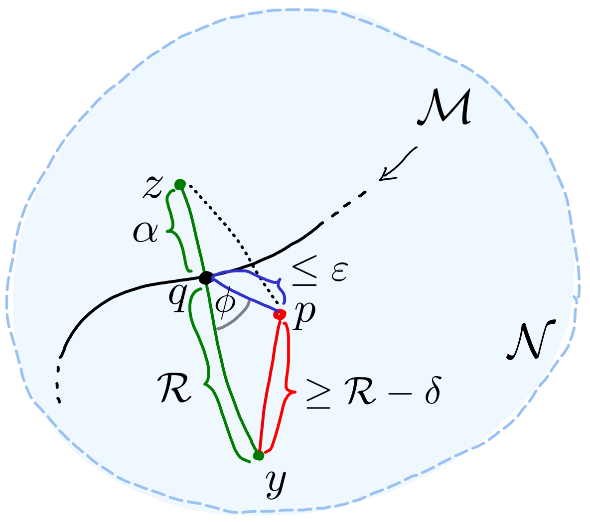
(b)

Figure 21: Overview of the notation used in the proof of Lemma B.11. On the right we see the two comparison triangles $ypq$ and $zpq$.

Further, let $v\in\mathrm{Nor}(q,\mathcal{M})\subseteq N_{q}\mathcal{M}\subseteq T_{q}\mathcal{N}$ . Denote the geodesic emanating from the point $q$ in direction $v$ by $\gamma_{q,v}$ and write $\gamma_{q,v}(\mathcal{R})=x$ and $\gamma_{q,-v}(\mathcal{R})=y$ . Thanks to Lemma B.6, the manifold $\mathcal{M}$ and the ball $B(x,\mathcal{R})^{\circ}$ (resp. $B(y,\mathcal{R})^{\circ}$) do not intersect, and thus

$$p\notin B(x,\mathcal{R}-\delta)^{\circ},\quad\text{as well as}\quad p\notin B(y,\mathcal{R}-\delta)^{\circ}.$$ (36)

Finally, write $\gamma_{q,v}(\alpha)=z$. Our goal is to upper bound the distance between the point $p$ and the point $z$. To this end, we consider two geodesic triangles: $ypq$ and $zpq$. We sketch the situation in Figure 21. The lengths of their edges satisfy:

$$d_{\mathcal{N}}(y,q)=\mathcal{R},\qquad d_{\mathcal{N}}(y,p)\geq\mathcal{R}-\delta,\qquad d_{\mathcal{N}}(p,q)\leq\varepsilon,\qquad d_{\mathcal{N}}(z,q)=\alpha.$$

In the remainder of the proof, we use the terminology and results from comparison theory, which we summarize in Appendix C. We first determine a lower bound $\phi_{\ell}$ on the angle $\phi=\angle yqp$, by applying Alexandrov-Toponogov angle comparison theorem (Theorem C.4) to the triangle $ypq$.

Having established a bound on the angle $\phi$, we apply Alexandrov-Toponogov distance comparison Theorem (Theorem C.3) to the triangle $qpz$. Since $\angle zqp=\pi-\phi$, Theorem C.3 gives us an upper bound on the length of the edge $pz$, which we denote by $r_{m}$. We stress that $\pi-\phi_{\ell}$ is an upper bound on the angle $\angle zqp$.

The length of the closing edge of a hinge in a space form is monotone in the lengths of the edges and the angle of the hinge, since, in the case when ${\Lambda_{\ell}}>0$, we can assume that $\mathcal{R}\leq\frac{\pi}{2\sqrt{{\Lambda_{\ell}}}}$.

Thus, $r_{m}$ is upper bounded by the closing edge of the hinge with edge lengths $\alpha$ and $\varepsilon$, and the angle $\pi-\phi_{\ell}$. Using the law of cosines for space forms (Proposition C.7) we deduce that $r_{m}$ satisfies

$$\cos\left(\sqrt{{\Lambda_{\ell}}}r_{m}\right)= \cos\left(\sqrt{{\Lambda_{\ell}}}\alpha\right)\cos\left(\sqrt{{\Lambda_{\ell}}}\varepsilon\right)$$

$$-\frac{\sin\left(\sqrt{{\Lambda_{\ell}}}\alpha\right)}{\sin\left(\sqrt{{\Lambda_{\ell}}}\mathcal{R}\right)}\left(\cos\left(\sqrt{{\Lambda_{\ell}}}(\mathcal{R}-\delta)\right)-\cos\left(\sqrt{{\Lambda_{\ell}}}\mathcal{R}\right)\cos\left(\sqrt{{\Lambda_{\ell}}}\varepsilon\right)\right),$$

$$= \frac{1}{\sin\left(\sqrt{{\Lambda_{\ell}}}\mathcal{R}\right)}\left[\sin\left(\sqrt{{\Lambda_{\ell}}}\left(\mathcal{R}+\alpha\right)\right)\cos\left(\sqrt{{\Lambda_{\ell}}}\varepsilon\right)-\sin\left(\sqrt{{\Lambda_{\ell}}}\alpha\right)\cos\left(\sqrt{{\Lambda_{\ell}}}(\mathcal{R}-\delta)\right)\right], {\Lambda_{\ell}}>0$$ (if )

$$r_{m}^{2}= \alpha^{2}+\varepsilon^{2}+\frac{\alpha}{\mathcal{R}}\left(\mathcal{R}^{2}+\varepsilon^{2}-(\mathcal{R}-\delta)^{2}\right), {\Lambda_{\ell}}=0$$ (if )

$$\cosh\left(\sqrt{{{\left\lvert{\Lambda_{\ell}}\right\rvert}}}r_{m}\right)= \cosh\left(\sqrt{{{\left\lvert{\Lambda_{\ell}}\right\rvert}}}\alpha\right)\cosh\left(\sqrt{{{\left\lvert{\Lambda_{\ell}}\right\rvert}}}\varepsilon\right)$$

$$-\frac{\sinh\left(\sqrt{{{\left\lvert{\Lambda_{\ell}}\right\rvert}}}\alpha\right)}{\sinh\left(\sqrt{{{\left\lvert{\Lambda_{\ell}}\right\rvert}}}\mathcal{R}\right)}\left(\cosh\left(\sqrt{{{\left\lvert{\Lambda_{\ell}}\right\rvert}}}(\mathcal{R}-\delta)\right)-\cosh\left(\sqrt{{{\left\lvert{\Lambda_{\ell}}\right\rvert}}}\mathcal{R}\right)\cosh\left(\sqrt{{{\left\lvert{\Lambda_{\ell}}\right\rvert}}}\varepsilon\right)\right)$$

$$= \frac{1}{\sinh\left(\sqrt{{{\left\lvert{\Lambda_{\ell}}\right\rvert}}}\mathcal{R}\right)}\left[\sinh\left(\sqrt{{{\left\lvert{\Lambda_{\ell}}\right\rvert}}}\left(\mathcal{R}+\alpha\right)\right)\cosh\left(\sqrt{{{\left\lvert{\Lambda_{\ell}}\right\rvert}}}\varepsilon\right)\right.$$

$$\left.-\sinh\left(\sqrt{{{\left\lvert{\Lambda_{\ell}}\right\rvert}}}\alpha\right)\cosh\left(\sqrt{{{\left\lvert{\Lambda_{\ell}}\right\rvert}}}(\mathcal{R}-\delta)\right)\right]. {\Lambda_{\ell}}<0$$ (if )

We are now ready to generalize Proposition 4.5. The philosophy of the proof is the same as in Proposition 5.3 — we combine the conditions of Theorem B.8 and the bounds of Lemma B.11. However, the involvement of trigonometric functions makes the analysis significantly more complicated.

See 5.4

Proof B.13.

We combine Theorem B.8 and Lemma B.11. To improve the readability of the formulas, we write $\tilde{x}=\sqrt{{{\left\lvert{\Lambda_{\ell}}\right\rvert}}}x$.

At first, we assume that ${\Lambda_{\ell}}>0$. Combining Equations (29) and (35) yields:

$$\frac{1}{\sin\tilde{\mathcal{R}}}\left[\sin\left(\tilde{\mathcal{R}}+\tilde{\alpha}\right)\cos\tilde{\varepsilon}-\sin\tilde{\alpha}\cos(\tilde{\mathcal{R}}-\tilde{\delta})\right]\geq\cos\tilde{r}_{m}\geq\frac{\cos\left(\tilde{\mathcal{R}}-\tilde{\delta}\right)}{\cos\left(\tilde{\mathcal{R}}-\tilde{\alpha}\right)}.$$ (38)

By multiplying both sides of the inequality by $\sin\tilde{\mathcal{R}}\cos\left(\tilde{\mathcal{R}}-\tilde{\alpha}\right)$ and subtracting $\sin\tilde{\mathcal{R}}\cos\left(\tilde{\mathcal{R}}-\tilde{\delta}\right)$, we obtain

$$0\leq\cos\tilde{\varepsilon}\left[\cos\left(\tilde{\mathcal{R}}-\tilde{\alpha}\right)\sin\left(\tilde{\mathcal{R}}+\tilde{\alpha}\right)\right]-\cos\left(\tilde{\mathcal{R}}-\tilde{\delta}\right)\left[\cos\left(\tilde{\mathcal{R}}-\tilde{\alpha}\right)\sin\tilde{\alpha}+\sin\tilde{\mathcal{R}}\right].$$ (39)

Observe that the terms are neatly divided: We have one term with $\tilde{\varepsilon}$, followed by an expression involving $\tilde{\mathcal{R}}$ and $\tilde{\alpha}$ in square brackets, and one term with $\tilde{\mathcal{R}}-\tilde{\delta}$, followed again by an expression involving $\tilde{\mathcal{R}}$ and $\tilde{\alpha}$ in square brackets.

Using the standard sum and double angle formulas for trigonometric functions, we transform the terms in the square brackets into

$$\cos\left(\tilde{\mathcal{R}}-\tilde{\alpha}\right)\sin\left(\tilde{\mathcal{R}}+\tilde{\alpha}\right)=\frac{1}{2}\left[\sin 2\tilde{\alpha}+\sin 2\tilde{\mathcal{R}}\right]$$

and

$$\cos\left(\tilde{\mathcal{R}}-\tilde{\alpha}\right)\sin\tilde{\alpha}+\sin\tilde{\mathcal{R}}=\frac{1}{2}\left[\sin 2\tilde{\alpha}\cos\tilde{\mathcal{R}}+\sin\tilde{\mathcal{R}}\left(3-\cos 2\tilde{\alpha}\right)\right].$$

With this reformulation we extracted all expressions with $\tilde{\alpha}$. Denoting $x:=2\tilde{\alpha}$ we finally rearrange the inequality (39) in terms of $\cos x$ and $\sin x$:

$$0\leq\sin x\left[\cos\tilde{\varepsilon}-\cos\left(\tilde{\mathcal{R}}-\tilde{\delta}\right)\cos\tilde{\mathcal{R}}\right]+\cos x\left[\sin\tilde{\mathcal{R}}\cos\left(\tilde{\mathcal{R}}-\tilde{\delta}\right)\right]+\cos\tilde{\varepsilon}\sin 2\tilde{\mathcal{R}}-3\sin\tilde{\mathcal{R}}\cos\left(\tilde{\mathcal{R}}-\tilde{\delta}\right).$$

Recall that we want to determine conditions on $\varepsilon$ and $\delta$ (in terms of $\mathcal{R}$), under which there exists a value $x\in[0,\pi]$ that satisfies the inequality above. To this end, let

$$A:=\cos\tilde{\varepsilon}-\cos\left(\tilde{\mathcal{R}}-\tilde{\delta}\right)\cos\tilde{\mathcal{R}},$$

$$B:=\sin\tilde{\mathcal{R}}\cos\left(\tilde{\mathcal{R}}-\tilde{\delta}\right),$$

$$C:=\cos\tilde{\varepsilon}\sin 2\tilde{\mathcal{R}}-3\sin\tilde{\mathcal{R}}\cos\left(\tilde{\mathcal{R}}-\tilde{\delta}\right),$$

denote the three terms of the right hand side of the inequality. Observe that

$$A >0, B >0, C <0.$$ and (40)

Indeed, the inequalities

$$0\leq\tilde{\mathcal{R}}-\tilde{\delta}\leq\tilde{\mathcal{R}}\leq\pi/2\quad\text{and}\quad\varepsilon<\tilde{\mathcal{R}}$$

imply

$$0\leq\cos\tilde{\mathcal{R}}\leq\cos\left(\tilde{\mathcal{R}}-\tilde{\delta}\right)\quad\text{and}\quad\cos\tilde{\mathcal{R}}<\cos\varepsilon,$$

and thus

$$A =\cos\tilde{\varepsilon}-\cos\left(\tilde{\mathcal{R}}-\tilde{\delta}\right)\cos\tilde{\mathcal{R}}>\cos\tilde{\mathcal{R}}\left(1-\cos\left(\tilde{\mathcal{R}}-\tilde{\delta}\right)\right)\geq 0,$$

$$\tfrac{C}{\sin\tilde{\mathcal{R}}} =2\cos\tilde{\varepsilon}\cos\tilde{\mathcal{R}}-3\cos\left(\tilde{\mathcal{R}}-\tilde{\delta}\right)<\cos\tilde{\mathcal{R}}\left(2\cos\tilde{\varepsilon}-3\right)<0.$$

Define

$$f:[0,\pi]\to\mathbb{R},\qquad f(x)=A\sin x+B\cos x+C.$$

Our goal is to determine if there exists a point $x\in[0,\pi]$ with $f(x)\geq 0$. Consider $x_{0}\in[0,\pi]$ such that $\cos x_{0}=\frac{B}{\sqrt{A^{2}+B^{2}}}$ and $\sin x_{0}=\frac{A}{\sqrt{A^{2}+B^{2}}}$. With this definition we can rewrite $f(x)\geq 0$ as

$$f(x)=\sqrt{A^{2}+B^{2}}\left(\cos(x-x_{0})+\frac{C}{\sqrt{A^{2}+B^{2}}}\right)\geq 0.$$ (41)

We see that $f$ has only one global maximum value in the interval $[0,\pi]$, namely at $x_{0}$. Hence, there exists a point $x\in[0,\pi]$ with $f(x)\geq 0$ if and only if the global maximum $x_{0}$ of $f$ satisfies $f(x_{0})\geq 0$. This, in turns, translates into

$$1+\frac{C}{\sqrt{A^{2}+B^{2}}}\geq 0,$$

that is, $-C\leq\sqrt{A^{2}+B^{2}}$. Thanks to (40), this can be rewritten as $C^{2}\leq A^{2}+B^{2}$.

Plugging in the values of $A$, $B$, and $C$ yields

$$\left(2\cos\tilde{\varepsilon}\cos\tilde{\mathcal{R}}-3\cos\left(\tilde{\mathcal{R}}-\tilde{\delta}\right)\right)^{2}\leq\left(\frac{\cos\tilde{\varepsilon}-\cos\left(\tilde{\mathcal{R}}-\tilde{\delta}\right)\cos\tilde{\mathcal{R}}}{\sin\tilde{\mathcal{R}}}\right)^{2}+\cos^{2}\left(\tilde{\mathcal{R}}-\tilde{\delta}\right).$$ (8)

When ${\Lambda_{\ell}}=0$, the proof reduces to calculations identical to those in the proof of Proposition 4.5. We refrain from repeating them here, and refer the reader back to the proof.

Finally, we assume that ${\Lambda_{\ell}}<0$. Our procedure is identical to the treatment of the case where ${\Lambda_{\ell}}>0$. Combining Equations (29) and (35) yields:

$$\frac{1}{\sinh\tilde{\mathcal{R}}}\left[\sinh\left(\tilde{\mathcal{R}}+\tilde{\alpha}\right)\cosh\tilde{\varepsilon}-\sinh\tilde{\alpha}\cosh(\tilde{\mathcal{R}}-\tilde{\delta})\right]\leq\cosh\tilde{r}_{m}\leq\frac{\cosh\left(\tilde{\mathcal{R}}-\tilde{\delta}\right)}{\cosh\left(\tilde{\mathcal{R}}-\tilde{\alpha}\right)}.$$ (42)

By multiplying both sides of the inequality by $\sinh\tilde{\mathcal{R}}\cosh\left(\tilde{\mathcal{R}}-\tilde{\alpha}\right)$ and subtracting $\sinh\tilde{\mathcal{R}}\cosh\left(\tilde{\mathcal{R}}-\tilde{\delta}\right)$, we obtain

$$0\geq\cosh\tilde{\varepsilon}\left[\cosh\left(\tilde{\mathcal{R}}-\tilde{\alpha}\right)\sinh\left(\tilde{\mathcal{R}}+\tilde{\alpha}\right)\right]-\cosh\left(\tilde{\mathcal{R}}-\tilde{\delta}\right)\left[\cosh\left(\tilde{\mathcal{R}}-\tilde{\alpha}\right)\sinh\tilde{\alpha}+\sinh\tilde{\mathcal{R}}\right].$$ (43)

We transform the terms in the square brackets into

$$\cosh\left(\tilde{\mathcal{R}}-\tilde{\alpha}\right)\sinh\left(\tilde{\mathcal{R}}+\tilde{\alpha}\right)=\frac{1}{2}\left[\sinh 2\tilde{\alpha}+\sinh 2\tilde{\mathcal{R}}\right]$$

and

$$\cosh\left(\tilde{\mathcal{R}}-\tilde{\alpha}\right)\sinh\tilde{\alpha}+\sinh\tilde{\mathcal{R}}=\frac{1}{2}\left[\sinh 2\tilde{\alpha}\cosh\tilde{\mathcal{R}}+\sinh\tilde{\mathcal{R}}\left(3-\cosh 2\tilde{\alpha}\right)\right].$$

Denoting $x:=2\tilde{\alpha}$ we finally rearrange the inequality (43) into a polynomial in $\cosh x$ and $\sinh x$:

$$0\geq \sinh x\left[\cosh\tilde{\varepsilon}-\cosh\left(\tilde{\mathcal{R}}-\tilde{\delta}\right)\cosh\tilde{\mathcal{R}}\right]+\cosh x\left[\cosh\left(\tilde{\mathcal{R}}-\tilde{\delta}\right)\sinh\tilde{\mathcal{R}}\right]$$

$$\quad+\cosh\tilde{\varepsilon}\sinh 2\tilde{\mathcal{R}}-3\sinh\tilde{\mathcal{R}}\cosh\left(\tilde{\mathcal{R}}-\tilde{\delta}\right).$$

Recall that we want to determine conditions on $\varepsilon$ and $\delta$ (in terms of $\mathcal{R}$), under which there exists a value $x\geq 0$ that satisfies the inequality above. To this end, let

$$A_{h}:=\cosh\tilde{\varepsilon}-\cosh\left(\tilde{\mathcal{R}}-\tilde{\delta}\right)\cosh\tilde{\mathcal{R}},$$

$$B_{h}:=\sinh\tilde{\mathcal{R}}\cosh\left(\tilde{\mathcal{R}}-\tilde{\delta}\right),$$

$$C_{h}:=\cosh\tilde{\varepsilon}\sinh 2\tilde{\mathcal{R}}-3\sinh\tilde{\mathcal{R}}\cosh\left(\tilde{\mathcal{R}}-\tilde{\delta}\right),$$

denote the three terms of the right hand side of the inequality. Observe that

$$A_{h}<0,\qquad B_{h}>0,\qquad\text{and}\qquad A_{h}+B_{h}>0.$$

Indeed, the inequality $0\leq\tilde{\varepsilon}<\tilde{\mathcal{R}}$ implies $\cosh\tilde{\varepsilon}<\cosh\tilde{\mathcal{R}}$, and thus

$$A_{h} =\cosh\tilde{\varepsilon}-\cosh\left(\tilde{\mathcal{R}}-\tilde{\delta}\right)\cosh\tilde{\mathcal{R}}<\cosh\tilde{\mathcal{R}}\left(1-\cosh\left(\tilde{\mathcal{R}}-\tilde{\delta}\right)\right)\leq 0,$$

$$A_{h}+B_{h} =\cosh\tilde{\varepsilon}-e^{-\tilde{\mathcal{R}}}\cosh\left(\tilde{\mathcal{R}}-\tilde{\delta}\right)\geq\cosh\tilde{\varepsilon}-e^{-\tilde{\mathcal{R}}}\cosh\tilde{\mathcal{R}}=\cosh\tilde{\varepsilon}-\tfrac{1}{2}\left(1+e^{-2\tilde{\mathcal{R}}}\right)>0.$$

Define

$$g:[0,\infty)\to\mathbb{R},\qquad g(x)=A_{h}\sinh x+B_{h}\cosh x+C_{h}.$$

Because $A_{h}+B_{h}>0$, we have that $B_{h}^{2}-A_{h}^{2}>0$. We now define $\rho$ to be the positive solution of the equations

$$\rho^{2}=B_{h}^{2}-A_{h}^{2}.$$

Because $\cosh^{2}(x)-\sinh^{2}(x)=1$ and $0\leq-A_{h}<B_{h}$, there exists an $x_{0}$ such that $-A_{h}=\rho\sinh x_{0}$ and $B_{h}=\rho\cosh x_{0}$. Indeed, $x_{0}$ is given by $x_{0}=\arctan(-A_{h}/B_{h})$. Using the sum formula for $\cosh(a-b)$ we get the condition

$$\frac{1}{\rho}g(x)=\cosh(x-x_{0})+\frac{C_{h}}{\rho}\leq 0.$$ (44)

Since the minimum of $t\mapsto\cosh t$ is $1$, this condition reduces to $\frac{C_{h}}{\rho}\leq-1$, or equivalently

$$C_{h}\leq-\sqrt{B_{h}^{2}-A_{h}^{2}}.$$ (45)

It is not difficult to recover the interval where $g(x)\leq 0$ from (44). It is convenient to reformulate (45) as

$$C_{h}\leq 0\qquad\text{and}\qquad B_{h}^{2}\leq A_{h}^{2}+C_{h}^{2}.$$

In terms of $\tilde{\varepsilon},\tilde{\delta}$, and $\tilde{\mathcal{R}}$, these inequalities are equivalent to

$$2\cosh\tilde{\varepsilon}\cosh\tilde{\mathcal{R}} \leq 3\cosh\left(\tilde{\mathcal{R}}-\tilde{\delta}\right)\qquad\text{and}\qquad$$

$$\cosh^{2}\left(\tilde{\mathcal{R}}-\tilde{\delta}\right) \leq\left(\frac{\cosh\tilde{\varepsilon}-\cosh\left(\tilde{\mathcal{R}}-\tilde{\delta}\right)\cosh\tilde{\mathcal{R}}}{\sinh\tilde{\mathcal{R}}}\right)^{2}+\left(2\cosh\tilde{\varepsilon}\cosh\tilde{\mathcal{R}}-3\cosh\left(\tilde{\mathcal{R}}-\tilde{\delta}\right)\right)^{2}.$$ (9)

B.4 Tightness of the bounds on the sampling parameters

We now prove that the bounds in the Riemannian setting are also tight in the following sense:

Proposition B.14.

Let ${\Lambda_{\ell}}\in\mathbb{R}$. Assume that the one-sided Hausdorff distances $\varepsilon$ and $\delta$ fail to satisfy bound (6). Then there exists a manifold $\mathcal{N}$ (namely a space form) of dimension $d\geq 2$ whose sectional curvatures satisfy $K\geq{\Lambda_{\ell}}$ (in fact $K={\Lambda_{\ell}}$), a subset ${\mathcal{S}}\subseteq\mathcal{N}$ of positive (cut locus) reach $\mathcal{R}$, and a sample $P$ that satisfy Universal Assumption 5.1, while the homology of the union of balls $P^{\boxplus r}$ does not equal the homology of ${\mathcal{S}}$ for any $r$.

Proposition B.15.

Let ${\Lambda_{\ell}}\in\mathbb{R}$. Assume moreover that the one-sided Hausdorff distances $\varepsilon$ and $\delta$ fail to satisfy bound (8), and $\delta\leq\varepsilon$. Then there exists a manifold $\mathcal{N}$ (namely a space form) of dimension $d\geq 3$ whose sectional curvatures satisfy $K\geq{\Lambda_{\ell}}$ (in fact $K={\Lambda_{\ell}}$), a submanifold $\mathcal{M}\subseteq\mathcal{N}$ of positive (cut locus) reach, and a sample $P$ that satisfy Universal Assumption 5.1, while the homology of the union of balls $P^{\boxplus r}$ does not equal the homology of $\mathcal{M}$ for any $r$.

As in Section 4.4, we prove Propositions B.14 and B.15 by an explicit construction. We construct the set ${\mathcal{S}}$, the manifold $\mathcal{M}$, and the corresponding samples in Examples B.18 and B.22, respectively.

Remark B.16.

As in Section 4.4, our construction involves a large (but finite) number of annuli or tori in a space form. If the curvature of the space form is positive then its volume is finite, such as in Figure 22. To be able to accommodate all the annuli, resp. tori, in our space form, we have to assume that it consists of multiple connected components.

Instead of resorting to multiple connected components one could also weaken the statement as follows:

Proposition B.17.

Let ${\Lambda_{\ell}}\in\mathbb{R}$. Assume that the one-sided Hausdorff distances $\varepsilon$ and $\delta$ fail to satisfy bound (6) ((8) respectively). Then there exists no $r$ such that

• for any manifold $\mathcal{N}$ of dimension $d\geq 2$ ($d\geq 3$ respectively), whose sectional curvatures satisfy $K\geq{\Lambda_{\ell}}$,

• for any a subset ${\mathcal{S}}\subseteq\mathcal{N}$ of positive cut locus reach $\mathcal{R}$ (for every manifold $\mathcal{M}\subseteq\mathcal{N}$ of positive cut locus reach $\mathcal{R}$, respectively), and

• for any sample $P$ that satisfies Universal Assumption 5.1

the homology of the union of balls $P^{\boxplus r}$ equals the homology of ${\mathcal{S}}$ ($\mathcal{M}$ respectively).

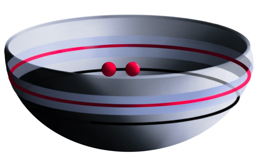
Figure 22: An illustration of an annulus (in blue) on the sphere (in gray, we depict only half the sphere for the visualization) as well as the sample $P$ (in red). It is clear from the figure that the annulus takes up so much space that placing another one in the same sphere is impossible.

B.4.1 Subsets of Riemannian manifolds with positive reach

The construction of example in a space form of non-zero curvature, with which we prove Proposition B.14, generalizes the construction in Euclidean space (Example A.19) quite directly, see Figure 23.

Example B.18.

We choose $\mathcal{N}$ to be a two-dimensional space form of curvature ${\Lambda_{\ell}}$, which we denote by $\mathbb{H}^{2}({\Lambda_{\ell}})$. The set ${\mathcal{S}}$ is a union of annuli, where by an annulus $A_{i}$ we mean a set $A_{i}=B(z_{i},\mathcal{R}+{2}\varepsilon)\setminus B^{\circ}(z_{i},\mathcal{R})\subseteq\mathbb{H}^{2}({\Lambda_{\ell}})$. We call the point $z_{i}\in\mathbb{H}^{2}({\Lambda_{\ell}})$ the centre of the annulus. We assume the annuli lie at a distance at least $2\mathcal{R}$ away from each other.

The sample consists of a geodesic circle $C_{i}=\partial B(z_{i},\mathcal{R}+\varepsilon)$ and two points $\{p_{i},\tilde{p}_{i}\}\subseteq\partial B(z_{i},\mathcal{R}-\delta)$ that are separated by a distance $2r_{i}$ for each annulus $A_{i}$. We provide an explicit definition for the parameter $r_{i}$ shortly.

We recall that bisectors in $\mathbb{H}^{2}({\Lambda_{\ell}})$ are geodesics. Thus, the bisector of the points $p_{i}$ and $\tilde{p}_{i}$ intersects the circle $C_{i}$ in two points. We let $q_{i}$ be the intersection point that is the closest to $p_{i}$ (and thus $\tilde{p}_{i}$).

Consider the triangle $p_{i}\tilde{p}_{i}q_{i}$. We denote its circumradius by $R_{i}$ and note that $R_{i}\geq r_{i}$. Finally, we define the distance $2r_{i}$ between each pair of points $p_{i}$ and $\tilde{p}_{i}$: We set the distance $r_{0}$ to be

$$r_{0}=\tfrac{1}{2}d\left(q_{0},\tilde{q}_{0}\right),$$

and define

$$r_{i+1}=\begin{cases}R_{i},&\text{if }R_{i}<1-\delta,\\ 1-\delta,&\text{otherwise}.\end{cases}$$

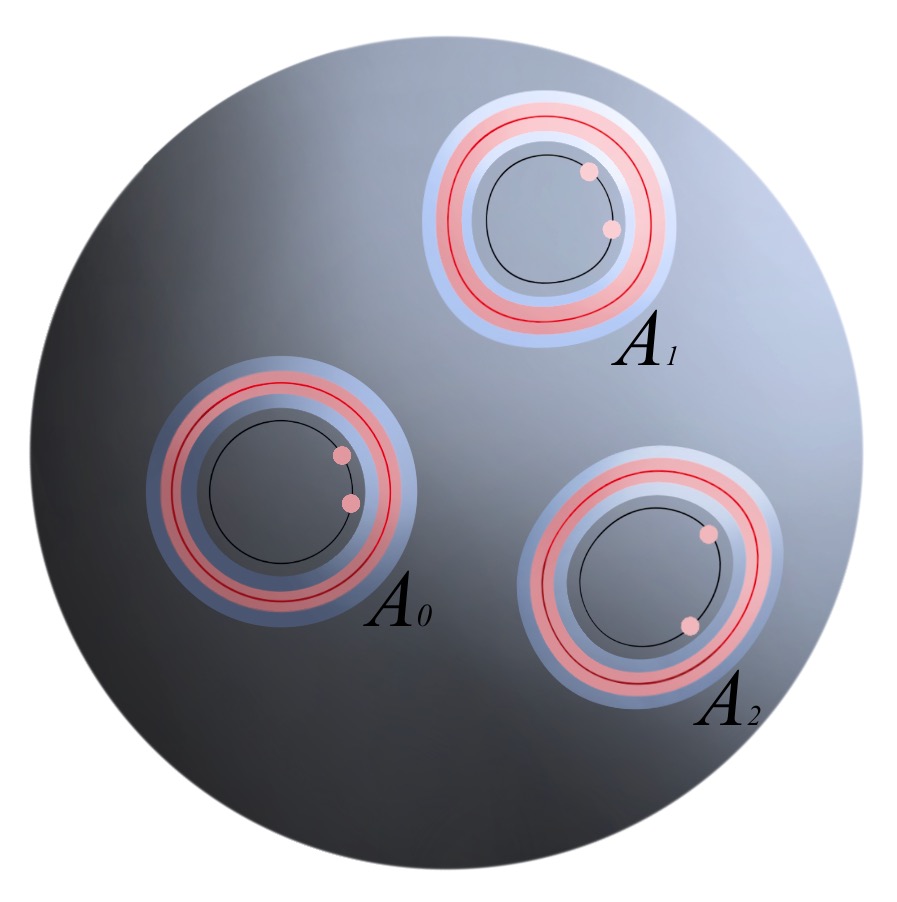
Figure 23: A sequence of annuli on a space form.

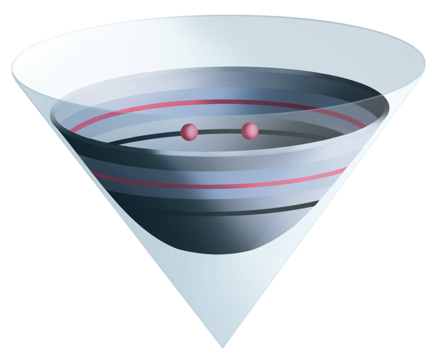
Figure 24: A single annulus with sample in hyperbolic space, visualized using the Minkowski or hyperboloid model [69]. The limiting cone of the hyperboloid is included in transparent light blue.

Next, we prove the generalization of Lemma A.20.

Lemma B.19.

If $\varepsilon$ and $\delta$ fail to satisfy the bound (6), then, for any $r_{i}\in[0,1-\delta]$,

• the triangle $p_{i}\tilde{p}_{i}q_{i}$ is strictly self-centred;

• there exists a constant $c>0$, depending only on $\delta$, $\varepsilon$, and ${\Lambda_{\ell}}$, such that $R_{i}-r_{i}\geq c\,r_{i}$.

Proof B.20.

We observe that the triangle $p_{i}\tilde{p}_{i}q_{i}$ is self-centred for a sufficiently small value of $r_{i}$ (see Figure 25).

Recall that the point $z_{i}$ is the centre of $C_{i}$, and let $C^{\prime}_{i}$ be the geodesic circle centred at $z_{i}$ with radius $\mathcal{R}-\delta$. That is,

$$C^{\prime}_{i}=\partial B(z_{i},\mathcal{R}-\delta).$$

By construction, the circle $C_{i}^{\prime}$ contains the points $p_{i}$ and $\tilde{p}_{i}$, while the circle $C_{i}$ contains the point $q_{i}$. Because the circumcentre of a triangle in a two-dimensional space lies on the bisector of any two of its vertices, the circumcentre of the triangle $p_{i}\tilde{p}_{i}q_{i}$ lies on the geodesic that contains the points $q_{i}$ and $z_{i}$ — the bisector of $p_{i}$ and $\tilde{p}_{i}$. By definition, the midpoint $\mu_{i}$ of the segment connecting $p_{i}$ and $\tilde{p}_{i}$ lies on the bisector of $p_{i}$ and $\tilde{p}_{i}$.

We observe that the triangle $p_{i}\tilde{p}_{i}q_{i}$ is (strictly) self-centred if and only if the distance $d(q_{i},\mu_{i})$ is (strictly) longer than the circumradius of $p_{i}\tilde{p}_{i}q_{i}$. In other words, the transition between self-centredness and non-self-centredness happens when $d(q_{i},\mu_{i})=d(p_{i},\mu_{i})=d(\tilde{p}_{i},\mu_{i})=r_{i}$.

We now consider the triangle $z_{i}q_{i}p_{i}$, which is right-angled. At the moment when the triangle $p_{i}\tilde{p}_{i}q_{i}$ transitions from self-centred to non-self-centred, the edge lengths of the triangle $z_{i}q_{i}p_{i}$ are $\mathcal{R}-\delta$, $\mathcal{R}+\varepsilon-r_{i}$, and $r_{i}$ (see Figure 25). Applying the law of cosines yields

$$\cos(\sqrt{{\Lambda_{\ell}}}(\mathcal{R}-\delta)) =\cos(\sqrt{{\Lambda_{\ell}}}(\mathcal{R}+\varepsilon-r_{i}))\cos(\sqrt{{\Lambda_{\ell}}}r_{i})$$

$$=\frac{1}{2}\left(\cos(\sqrt{{\Lambda_{\ell}}}(\mathcal{R}+\varepsilon))+\cos(\sqrt{{\Lambda_{\ell}}}(\mathcal{R}+\varepsilon-2r_{i}))\right), {\Lambda_{\ell}}>0$$ (if )

$$\cosh(\sqrt{{{\left\lvert{\Lambda_{\ell}}\right\rvert}}}(\mathcal{R}-\delta)) =\cosh(\sqrt{{{\left\lvert{\Lambda_{\ell}}\right\rvert}}}(\mathcal{R}+\varepsilon-r_{i}))\cosh(\sqrt{{{\left\lvert{\Lambda_{\ell}}\right\rvert}}}r_{i})$$

$$=\frac{1}{2}\left(\cosh(\sqrt{{{\left\lvert{\Lambda_{\ell}}\right\rvert}}}(\mathcal{R}+\varepsilon))+\cosh(\sqrt{{{\left\lvert{\Lambda_{\ell}}\right\rvert}}}(\mathcal{R}+\varepsilon-2r_{i}))\right), {\Lambda_{\ell}}<0$$ (if )

Thus, the triangle $p_{i}\tilde{p}_{i}q_{i}$ transitions between self-centred and non-self-centred if the above equations have a real solution. Finally, since for a sufficiently small value of $r_{i}$ the triangle $p_{i}\tilde{p}_{i}q_{i}$ is self-centred if there is no solution to the equation (LABEL:eq:conditionsTransitionPosReachRiemannMan), the triangle $p_{i}\tilde{p}_{i}q_{i}$ is self-centred for all $r_{i}\in[0,1-\delta]$.

The solution to (LABEL:eq:conditionsTransitionPosReachRiemannMan) being vacuous is equivalent to $\varepsilon$ and $\delta$ failing to satisfy the bound (6). This completes the proof of the first statement. We note that because the triangle $p_{i}\tilde{p}_{i}q_{i}$ is strictly self-centred, $R_{i}>r_{i}$ and the second statement of the lemma also follows.

Figure 25: The figure illustrates the positive curvature case.

Proof B.21 (Proof of Proposition B.14).

The example has been set up in such a way that the transitions of the homology are precisely the same as in the Euclidean setting, and as we have described in the proof of Proposition 4.6. Hence, the set ${\mathcal{S}}$ never has the same homology as the union of balls $\bigcup_{p\in P}B(p,r)$, and thus the two never have the same homotopy.

B.4.2 Submanifolds of Riemannian manifolds with positive reach

The construction of the submanifold of $\mathbb{H}^{d}({\Lambda_{\ell}})$ proving Proposition B.15 generalizes the construction of Example A.23.

Example B.22.

We choose $\mathcal{N}$ to be a three-dimensional space form of curvature ${\Lambda_{\ell}}$, which we denote by $\mathbb{H}^{3}({\Lambda_{\ell}})$, and define $\mathcal{M}\subseteq\mathbb{H}^{3}({\Lambda_{\ell}})$ to be a union of tori $T_{i}$. A geodesic circle $S^{1}(z,r)$ with centre $z$ and radius $r$ in a subspace $\mathbb{H}^{2}({\Lambda_{\ell}})\subseteq\mathbb{H}^{3}({\Lambda_{\ell}})$ is the boundary of a geodesic 2-ball (disk) $B(z,r)\subseteq\mathbb{H}^{2}({\Lambda_{\ell}})$. We write $H_{S}$ for the subspace $\mathbb{H}^{2}({\Lambda_{\ell}})\subseteq\mathbb{H}^{3}({\Lambda_{\ell}})$ that contains the circle $S^{1}(z,r)$. Whenever we want to express a circle in terms of the subspace $H_{S}$ it is lying in, we write $S^{1}(z,r,H_{S})$. We refer to $H_{S}$ as the symmetry plane. Finally, each of the tori $T_{i}$ is a $\mathcal{R}$-offset of the circle $S^{1}_{i}(z_{i},2\mathcal{R},H_{S})$ — a circle of radius $2\mathcal{R}$ in $\mathbb{H}^{3}({\Lambda_{\ell}})$. We refer to $z_{i}$ as the centre of the torus.

We number the tori from $i=0$, and we assume that their centres lie on a geodesic at a distance at least $2\mathcal{R}$ apart from one another, in such a way that they all share one symmetry plane $H_{S}$. Due to this assumption, the cut locus reach of $\mathcal{M}=\bigcup_{i}T_{i}$ equals $\mathcal{R}$.

The sample $P$ consists of sets $C_{i}$ which are tori with a part cut out, and pairs of points $\{p_{i},\tilde{p}_{i}\}$ lying inside the hole of each torus $T_{i}$. To construct each set $C_{i}$ we take the $\delta$-offset of the torus $T_{i}$, keep the part that lies inside the solid torus bounded by $T_{i}$, and remove an $\varepsilon$-neighbourhood of the circle $S^{1}(z,\mathcal{R},H_{S})$.

Each pair of points, $p_{i}$ and $\tilde{p}_{i}$, lies on the circle $S^{1}(z,\mathcal{R}-\delta,H_{S})$ at a distance $2r_{i}$ from each other. Let $q_{i}$ and $\tilde{q}_{i}$ be the two points in the intersection of the bisector of $p_{i}$ and $\tilde{p}_{i}$ and the set $C_{i}$ that lie closest to $p_{i}$ and $\tilde{p}_{i}$. Note that $q_{i}$ and $\tilde{q}_{i}$ lie on the boundary of $C_{i}$. We denote the circumradius of the simplex $p_{i}\tilde{p}_{i}q_{i}\tilde{q}_{i}$ by $R_{i}$.

As in the Euclidean setting, we define the distance $2r_{i}$ between each pair of points $p_{i}$ and $\tilde{p}_{i}$ inductively. We set the distance $r_{0}$ to be:

$$r_{0}=\tfrac{1}{2}d\left(q_{0},\tilde{q}_{0}\right).$$

Moreover, we define

$$r_{i+1}=\begin{cases}R_{i},&\text{if }R_{i}<1-\delta,\\ 1-\delta,&\text{otherwise}.\end{cases}$$

As before, we need a result on self-centredness of simplices.

Lemma B.23.

If $\varepsilon$ and $\delta$ fail to satisfy bound (8), and $r_{i}$ satisfies

$$r_{i} \leq 1-\delta, 2r_{i} \geq d(q_{i},\tilde{q}_{i}),$$ (19)

then

• the simplex $p_{i}\tilde{p}_{i}q_{i}\tilde{q}_{i}$ is strictly self-centred;

• there exists a constant $c>0$, depending only on $\delta$, $\varepsilon$ and ${\Lambda_{\ell}}$, such that $R_{i}\geq r_{i}+c$.

Figure 26: The figure illustrates the transition between self-centred and non-self-centred simplices in the Euclidean case. The blue circles lie in $H_{S}$.

Proof B.24.

By definition, the circumcentre of the simplex $p_{i}\tilde{p}_{i}q_{i}\tilde{q}_{i}$ lies on the bisector of $p_{i}$ and $\tilde{p}_{i}$ and the bisector of $q_{i}$ and $\tilde{q}_{i}$. Hence, the circumcentre of $p_{i}\tilde{p}_{i}q_{i}\tilde{q}_{i}$ lies on the geodesic $\gamma_{i}$ that contains the midpoint $\mu_{i}$ of $p_{i},\tilde{p}_{i}$, and $z_{i}$. For convenience we assume that $\gamma_{i}$ is arc length parametrized, that $\gamma_{i}(0)=z_{i}$, and that, for some parameter $t>0$, $\gamma_{i}([0,t])$ is the minimizing geodesic connecting the points $z_{i}$ and $\mu_{i}$. We write $Q=\gamma_{i}(\mathcal{R})$ and $\tilde{z}_{i}=\gamma_{i}(2\mathcal{R})$. Finally, we denote the midpoint of $q_{i}$ and $\tilde{q}_{i}$ by $\tilde{\mu_{i}}$, and note that $\tilde{\mu}_{i}\in\gamma_{i}$.

We start by noting that if $2r_{i}=d(q_{i},\tilde{q}_{i})$, the circumcentre of the simplex $p_{i}\tilde{p}_{i}q_{i}\tilde{q}_{i}$ is the midpoint of $\mu_{i}$ and $\tilde{\mu}_{i}$. Therefore, the simplex $p_{i}\tilde{p}_{i}q_{i}\tilde{q}_{i}$ is self-centred. We denote this midpoint by $\gamma_{i}(\tau)$. As we increase the value of the parameter $r_{i}$, the circumcentre of $p_{i}\tilde{p}_{i}q_{i}\tilde{q}_{i}$ moves along $\gamma_{i}$ in such a way that if we parametrize the movement by $\gamma_{i}(\tau^{\prime})$, the parameter $\tau^{\prime}$ decreases.

The transition between self-centredness and non-self-centredness of $p_{i}\tilde{p}_{i}q_{i}\tilde{q}_{i}$ takes place when the midpoint $\mu_{i}$ is the circumcentre of $p_{i}\tilde{p}_{i}q_{i}\tilde{q}_{i}$. This critical point is depicted in Figure 26. In this case, the distance between the points $q_{i}$ and $\mu_{i}$ equals $d(q_{i},\mu_{i})=r_{i}$, and, by symmetry, $d(q_{i},\mu_{i})=\tilde{r}_{i}$).

Let $\alpha^{\prime}=d(Q_{i},\mu_{i})$, and consider the two triangles $\mu_{i}Q_{i}q_{i}$ and $Q_{i}q_{i}\tilde{z}_{i}$ (or the symmetric triangles $\mu_{i}Q_{i}q_{i}$ and $Q_{i}q_{i}\tilde{z}_{i}$). Applying the law of cosines and using the fact that $\angle\mu_{i}Q_{i}q_{i}=\pi-\angle q_{i}Q_{i}\tilde{z}_{i}$ yields

$$\cos\left(\sqrt{{\Lambda_{\ell}}}r_{i}\right)= \cos\left(\sqrt{{\Lambda_{\ell}}}\alpha^{\prime}\right)\cos\left(\sqrt{{\Lambda_{\ell}}}\varepsilon\right),$$

$$+\frac{\sin\left(\sqrt{{\Lambda_{\ell}}}\alpha^{\prime}\right)}{\sin\left(\sqrt{{\Lambda_{\ell}}}\mathcal{R}\right)}\left(\cos\left(\sqrt{{\Lambda_{\ell}}}(\mathcal{R}-\delta)\right)-\cos\left(\sqrt{{\Lambda_{\ell}}}\mathcal{R}\right)\cos\left(\sqrt{{\Lambda_{\ell}}}\varepsilon\right)\right) {\Lambda_{\ell}}>0$$ (if )

$$\cosh\left(\sqrt{{{\left\lvert{\Lambda_{\ell}}\right\rvert}}}r_{i}\right)= \cosh\left(\sqrt{{{\left\lvert{\Lambda_{\ell}}\right\rvert}}}\alpha^{\prime}\right)\cosh\left(\sqrt{{{\left\lvert{\Lambda_{\ell}}\right\rvert}}}\varepsilon\right)$$

$$+\frac{\sinh\left(\sqrt{{{\left\lvert{\Lambda_{\ell}}\right\rvert}}}\alpha^{\prime}\right)}{\sinh\left(\sqrt{{{\left\lvert{\Lambda_{\ell}}\right\rvert}}}\mathcal{R}\right)}\left(\cosh\left(\sqrt{{{\left\lvert{\Lambda_{\ell}}\right\rvert}}}(\mathcal{R}-\delta)\right)-\cosh\left(\sqrt{{{\left\lvert{\Lambda_{\ell}}\right\rvert}}}\mathcal{R}\right)\cosh\left(\sqrt{{{\left\lvert{\Lambda_{\ell}}\right\rvert}}}\varepsilon\right)\right), {\Lambda_{\ell}}<0$$ (if )

Non-coincidentally, this expression is, up to relabeling of certain variables, the same as Equation (LABEL:eqdef:rm).

On the other hand, applying the law of cosines to the triangle $p_{i}\mu_{i}z_{i}$ (or symmetrically to $\tilde{p}_{i}\mu_{i}z_{i}$) yields

$$\cos\sqrt{{\Lambda_{\ell}}}(\mathcal{R}-\delta) =\cos\sqrt{{\Lambda_{\ell}}}r_{i}\cos\sqrt{{\Lambda_{\ell}}}(\mathcal{R}-\alpha^{\prime}), {\Lambda_{\ell}}>0$$ (if )

$$\cosh\sqrt{{{\left\lvert{\Lambda_{\ell}}\right\rvert}}}(\mathcal{R}-\delta) =\cosh\sqrt{{{\left\lvert{\Lambda_{\ell}}\right\rvert}}}r_{i}\cosh\sqrt{{{\left\lvert{\Lambda_{\ell}}\right\rvert}}}(\mathcal{R}-\alpha^{\prime}). {\Lambda_{\ell}}<0$$ (if )

Combining Equations (LABEL:eq:CritManRiem1) and (LABEL:eq:ConditionThirdTriangle) yields inequalities (38) and (42), with the inequality replaced by an equality, and $\alpha$ replaced by $\alpha^{\prime}$. A transition between self-centred and non-self-centred simplices can thus only take place if this equation has a real solution. The existence of this solution has been analyzed in the proof of Proposition 5.4, leading to the inequalities (8) and (9).

In summary, the simplex $p_{i}\tilde{p}_{i}q_{i}\tilde{q}_{i}$ is self-centred if the conditions (19) are satisfied.

Since, for any $\varepsilon$ and $\delta$ failing inequalities (8) and (9), the simplex $p_{i}\tilde{p}_{i}q_{i}\tilde{q}_{i}$ is strictly self-centred for all $r\in\left[\frac{d(q_{i},\tilde{q})}{2},1-\delta\right]$, there is a lower bound on the difference between the length $2r_{i}$ of the edge $p_{i}\tilde{p}_{i}$ and the circumradius of the simplex $p_{i}\tilde{p}_{i}q_{i}\tilde{q}_{i}$. From this we deduce the second claim of the lemma.

Proof B.25 (Proof of Proposition B.15).

The example has been set up in such a way that the transitions of the homology are precisely the same as in the Euclidean setting, and as we have described in the proof of Proposition 4.7. Once again, the manifold $\mathcal{M}$ never has the same homology as the union of balls $\bigcup_{p\in P}B(p,r)$, and thus the two never have the same homotopy.

Appendix II: Additional material

Appendix C The Toponogov comparison theorem and spaces of constant curvature

We rely on the Toponogov comparison theorems and the geometry of spaces of constant curvature. In this appendix we recall the results we use, however for the reader that is completely unfamiliar with the topic it may help to also take a look at the pedagogical overview in [16].

We use the notation $\mathbb{H}(\Lambda)$ for the complete, simply connected space of dimension $2$ with constant sectional curvature $\Lambda$. A complete simply connected space with constant sectional curvature is also called a space form. Unless we state differently we assume a space of constant curvature to mean a space form.

The $2$-dimensional space of constant curvature $\Lambda$ is, explicitly [16, Theorem 39, pp. 228]:

$$\mathbb{H}(\Lambda)=\begin{cases}\frac{1}{\sqrt{-\Lambda}}\mathbb{HYP}^{2}&\text{if}\quad\Lambda<0\\ \mathbb{E}^{2}&\text{if}\quad\Lambda=0\\ \frac{1}{\sqrt{\Lambda}}\mathbb{S}^{2}&\text{if}\quad\Lambda>0.\end{cases}$$ (49)

where $\mathbb{HYP}^{2}$, $\mathbb{E}^{2}$ and $\mathbb{S}^{2}$ denote, respectively, the $2$-dimensional hyperbolic space, Euclidean space and sphere.

We are now ready to make the following definitions.

Definition C.1 (Geodesic triangle).

A geodesic triangle $ABC$ in a Riemannian manifold $\mathcal{N}$ consists of three minimizing geodesics connecting the three points $A,B,C$, sometimes also referred to as vertices. (We stress that a geodesic triangle does not include an interior.)

Complete Riemannian manifolds with positive lower bound on sectional curvature have bounded diameter [16, Theorem 62, pp. 266]:

Theorem C.2 (Bonnet-Schoenberg-Myers theorem).

If a complete Riemannian manifold $\mathcal{N}$ has sectional curvature $K$ bounded below by a positive constant ${\Lambda_{\ell}}$:

$$0<{\Lambda_{\ell}}\leq K,$$

then it satisfies:

$$\operatorname{diam}(\mathcal{N})\leq\frac{\pi}{\sqrt{{\Lambda_{\ell}}}}.$$ (50)

The next two theorems are adapted from [24, Theorems IX.5.1 and IX.5.2]. Since, unlike in [24], our definition of geodesic triangles requires each edge to be a minimizing geodesic, and thanks to (50), the statements in [24] can be simplified.

Theorem C.3 (Alexandrov-Toponogov distance comparison theorem).

Let $\mathcal{N}$ be a complete Riemannian manifold with sectional curvatures bounded below by ${\Lambda_{\ell}}$.

Let $ABC$ be a geodesic triangle in $\mathcal{N}$. Let us denote by $a$,$b$,and $c$ the respective lengths of sides $BC$,$CA$, and $AB$, and by $\alpha$ the angle at vertex $A$ (see Figure 27). Then there exists a geodesic triangle $A^{\prime}B^{\prime}C^{\prime}$ in $\mathbb{H}({\Lambda_{\ell}})$ such that sides $A^{\prime}B^{\prime}$ and $A^{\prime}C^{\prime}$ have respective lengths $c$ and $b$ and whose angle at $A^{\prime}$ is $\alpha$. If $a^{\prime}$ is the length of edge $B^{\prime}C^{\prime}$, then:

$$a\leq a^{\prime}$$

Theorem C.4 (Alexandrov-Toponogov angle comparison theorem).

Let $\mathcal{N}$ be a complete Riemannian manifold with sectional curvatures bounded below by ${\Lambda_{\ell}}$.

Let $ABC$ be a geodesic triangle in $\mathcal{N}$. Let us denote by $a$,$b$,and $c$ the respective lengths of sides $BC$,$CA$, and $AB$, and by $\alpha$, $\beta$ and $\gamma$ the respective angles at vertex $A$, $B$, and $C$ (see Figure 27).

Then there exists a geodesic triangle $A^{\prime}B^{\prime}C^{\prime}$ in $\mathbb{H}({\Lambda_{\ell}})$ such that sides $B^{\prime}C^{\prime}$,$C^{\prime}A^{\prime}$, and $A^{\prime}B^{\prime}$ have respective lengths $a$,$b$, and $c$, and, if $\alpha^{\prime}$, $\beta^{\prime}$ and $\gamma^{\prime}$ are the respective angles at vertex $A^{\prime}$, $B^{\prime}$, and $C^{\prime}$, then:

$$\alpha \geq\alpha^{\prime}$$

$$\beta \geq\beta^{\prime}$$

$$\gamma \geq\gamma^{\prime}.$$

Unless ${\Lambda_{\ell}}>0$, and one of side lengths $a$,$b$, or $c$, is $\frac{\pi}{\sqrt{{\Lambda_{\ell}}}}$, the triangle $A^{\prime}B^{\prime}C^{\prime}$ is uniquely determined, up to isometries.

Figure 27: Triangle with the standard symbols for angles and lengths.

Remark C.5.

The case, in Theorem C.4, where ${\Lambda_{\ell}}>0$, and one of side lengths $a$,$b$, or $c$, is $\frac{\pi}{\sqrt{{\Lambda_{\ell}}}}$ can be ignored, in light of (50), if the sectional curvature is assumed bounded below by some ${\Lambda_{\ell}}^{\prime}>{\Lambda_{\ell}}$, where ${\Lambda_{\ell}}^{\prime}$ can be chosen arbitrarily close to ${\Lambda_{\ell}}$.

Remark C.6.

Propositions similar to Theorems C.3 and C.4 hold for manifolds with upper bounded sectional curvature, that imply reversed inequalities, but they require additional conditions, in particular for the edge lengths to not exceed the injectivity radius.

Theorem C.3 will be combined with the law of cosines for spaces of constant curvature.

Proposition C.7 (Law of cosines).

We consider a geodesic triangle $ABC$ in $\mathbb{H}({\Lambda_{\ell}})$. We denote by $a=\operatorname{length}(BC)$, $b=\operatorname{length}(CA)$ and $c=\operatorname{length}(AB)$ the side lengths and by $\alpha$ the angle at vertex $A$, as pictured on Figure 27.

In the hyperbolic case, that is when $\Lambda<0$, then:

$$\cosh\sqrt{|\Lambda|}a=\cosh\sqrt{|\Lambda|}c\>\cosh\sqrt{|\Lambda|}b\,-\,\sinh\sqrt{|\Lambda|}c\>\sinh\sqrt{|\Lambda|}b\>\cos\alpha$$

In the Euclidean case, that is when $\Lambda=0$, then:

$$a^{2}=c^{2}+b^{2}-2\,c\,b\cos\alpha$$

In the spherical case, that is when $\Lambda>0$, then:

$$\cos\sqrt{\Lambda}a=\cos\sqrt{\Lambda}c\>\cos\sqrt{\Lambda}b\,+\,\sin\sqrt{\Lambda}c\>\sin\sqrt{\Lambda}b\>\cos\alpha$$

Appendix D Bounds on the reach of submanifolds of Riemannian manifolds with positive lower bound on the curvature

In Theorem B.8 we have used the Bonnet-Schoenberg-Myers theorem (Theorem C.2) to prove that the reach of a set in a Riemannian manifold with positive curvature ${\Lambda_{\ell}}$ is upper bounded by $\frac{\pi}{\sqrt{{\Lambda_{\ell}}}}$. In this section we improve this bound by a factor of two in the case where the set in question is a manifold. The proof adjusts the argument for the Bonnet-Schoenberg-Myers theorem as given in [16, Theorem 62]. For this, we need to recall notation and a result from [16, Section 6.2].

Let $[a,b]\subseteq\mathbb{R}$ be an interval in $\mathbb{R}$, and $t\in[a,b]$. Following Berger [16], we write $c_{\alpha}(t)=c(\alpha,t)$ for a family of curves neighbouring a geodesic $\gamma(t)=c_{0}(t)$. The infinitesimal displacement is denoted by

$$Y(t)=\frac{\partial c}{\partial\alpha}\bigg{|}_{\alpha=0}.$$

We assume that the displacement is orthogonal to the geodesic. We denote the sectional curvature for the directions $v,w$ by $K(v,w)$, and write $\nabla_{t}$ for the covariant derivative. If the endpoints of $c_{\alpha}$ are fixed then [16, Equation (6.7)]

$$\frac{\partial^{2}\text{length}\,c_{\alpha}}{\partial\alpha^{2}}\bigg{|}_{\alpha=0}=\int_{a}^{b}\left(\|\nabla_{t}Y(t)\|^{2}-K(\gamma^{\prime}(t),Y(t))\|Y(t)\|^{2}\right)\mathrm{d}t.$$ (51)

If the endpoints are not fixed, Equation (51) gains an additional term [24, Theorem II.4.3]:

$$\frac{\partial^{2}\text{length}\,c_{\alpha}}{\partial\alpha^{2}}\bigg{|}_{\alpha=0}=\langle\nabla_{\alpha}\partial_{\alpha}c(\alpha,t)\mid_{\alpha=0},\gamma^{\prime}(t)\rangle\mid^{t=b}_{t=a}+\int_{a}^{b}\left(\|\nabla_{t}Y(t)\|^{2}-K(\gamma^{\prime}(t),Y(t))\|Y(t)\|^{2}\right)\mathrm{d}t.$$ (52)

Naturally, if the endpoints of $c_{\alpha}$ are not fixed, the first variation is non-zero (see [24, Theorem II.4.1]) and, using that $\gamma$ is a geodesic, we have

$$\frac{\partial\text{length}\,c_{\alpha}}{\partial\alpha}\bigg{|}_{\alpha=0}=\langle Y(t),\gamma^{\prime}(t)\rangle\mid^{t=b}_{t=a}.$$ (53)

Lemma D.1.

Suppose that the sectional curvatures of a Riemannian manifold $\mathcal{N}$ are lower bounded by ${\Lambda_{\ell}}>0$. Let $\mathcal{M}\subseteq\mathcal{N}$ be a $C^{2}$ submanifold of $\mathcal{N}$ of dimension and codimension at least one, with cut locus reach $\operatorname{cl}_{\mathcal{N}}(\mathcal{M})>0$. Then,

$$\mathrm{rch}^{\operatorname{cl}}_{\mathcal{N}}(\mathcal{M})\leq\frac{\pi}{2\sqrt{{\Lambda_{\ell}}}}.$$

Figure 28: The figure illustrates the notation used in Appendix D. The second order behaviour of $c_{\alpha}(t)$ is determined by the vector $W$. However, $W$ is not indicated in the figure.

Proof D.2.

To derive a contradiction assume that $\mathrm{rch}^{\operatorname{cl}}_{\mathcal{N}}(\mathcal{M})>\frac{\pi}{2\sqrt{{\Lambda_{\ell}}}}$. For any point $p\in\mathcal{N}\setminus\mathcal{M}$ sufficiently close to $\mathcal{M}$, the minimizing geodesic from $p$ to $\mathcal{M}$ has a tangent vector that is normal to $\mathcal{M}$ at the endpoint of the geodesic. Let us call this endpoint $q\in\mathcal{M}$, set $L=2\mathrm{rch}^{\operatorname{cl}}_{\mathcal{N}}(\mathcal{M})$, and parametrize the geodesic by a map

$$\gamma:\left[-\tfrac{L}{2},\tfrac{L}{2}\right]\to\mathcal{N}$$

in such a way that $\gamma$ is arc length parametrized and $\gamma(0)=q$. We refer to Figure 28 for an overview of the notation used. Furthermore, pick a tangent vector $Z\in T_{q}\mathcal{M}\subseteq T_{q}\mathcal{N}$. Due to the definition of $\gamma$, the vectors $Z$ and $\gamma^{\prime}(0)$ are perpendicular.

As in the proof of [16, Theorem 62], we then consider the parallel transport of $Z$ along $\gamma$, which we denote by $Z(t)$. With $L=2\mathrm{rch}^{\operatorname{cl}}_{\mathcal{N}}(\mathcal{M})$, we define

$$Y:\left[-\tfrac{L}{2},\tfrac{L}{2}\right]\to T\mathcal{N},\qquad Y(t)=\cos\left(\tfrac{\pi t}{L}\right)Z(t).$$

We choose the second order derivative of $c(\alpha,t)$ with respect to $\alpha$ as follows. We write $\eta(\alpha)$ for the geodesic in $\mathcal{M}$ emanating from $q$ in the direction $Z$, i.e., $\eta(0)=q$ and $\eta^{\prime}(0)=Z$. Next, we set

$$W:=\nabla_{\alpha}\eta^{\prime}(\alpha)\mid_{\alpha=0}$$

and, as with the vector $Z$, use parallel transport along $\gamma$ to extend the vector $W$ to a vector field $W(t)$ along the entire length of $\gamma$. Finally, we impose that

$$\nabla_{\alpha}\partial_{\alpha}c(\alpha,t)\mid_{\alpha=0}=\cos\left(\tfrac{\pi t}{L}\right)W(t).$$

We stress that, since the vector $Z$ lies in the tangent space $T_{q}\mathcal{M}$ and due to the way the vector field $W(t)$ is defined, the members of the family of curves $c_{\alpha}$ arising from $Y(t)$ pass (up to second order) through $\mathcal{M}$.

Finally, write $\psi_{\alpha}(t)$ for the restriction of $c_{\alpha}(t)$ to the interval $\left[-\tfrac{L}{2},0\right]$, and $\tilde{\psi}_{\alpha}(t)$ for the restriction of $c_{\alpha}(t)$ to the interval $\left[0,\tfrac{L}{2}\right]$. With this notation, and applying $L=2\mathrm{rch}^{\operatorname{cl}}_{\mathcal{N}}(\mathcal{M})>\frac{\pi}{\sqrt{{\Lambda_{\ell}}}}$, Equation (52) yields

$$\frac{\partial^{2}\text{length}\,\psi_{\alpha}(t)}{\partial\alpha^{2}}\bigg{|}_{\alpha=0} =\langle\nabla_{\alpha}\partial_{\alpha}c(\alpha,t)\mid_{\alpha=0},\gamma^{\prime}(t)\rangle\mid^{t=0}_{t=-L/2}$$

$$\phantom{=}+\int_{-L/2}^{0}\left(\frac{\pi^{2}}{L^{2}}\sin^{2}\left(\frac{\pi t}{L}\right)\|Z\|{{}^{2}}-K(\gamma^{\prime}(t),Y(t))\cos^{2}\left(\frac{\pi t}{L}\right)\|Z\|{{}^{2}}\right)\mathrm{d}t$$

$$\leq\langle W,\gamma^{\prime}(0)\rangle$$

$$\phantom{=}+\int_{-L/2}^{0}\left(\frac{\pi^{2}}{L^{2}}\sin^{2}\left(\frac{\pi t}{L}\right)\|Z\|{{}^{2}}-{\Lambda_{\ell}}\cos^{2}\left(\frac{\pi t}{L}\right)\|Z\|{{}^{2}}\right)\mathrm{d}t$$

$$=\langle W,\gamma^{\prime}(0)\rangle+\frac{L\|Z\|{{}^{2}}}{4}\left(\frac{\pi^{2}}{L^{2}}-{\Lambda_{\ell}}\right)$$

$$<\langle W,\gamma^{\prime}(0)\rangle,$$

and

$$\frac{\partial^{2}\text{length}\,\tilde{\psi}_{\alpha}(t)}{\partial\alpha^{2}}\bigg{|}_{\alpha=0} =\langle\nabla_{\alpha}\partial_{\alpha}c(\alpha,t)\mid_{\alpha=0},\gamma^{\prime}(t)\rangle\mid^{t=L/2}_{t=0}$$

$$\phantom{=}+\int_{0}^{L/2}\left(\frac{\pi^{2}}{L^{2}}\sin^{2}\left(\frac{\pi t}{L}\right)\|Z\|{{}^{2}}-K(\gamma^{\prime}(t),Y(t))\cos^{2}\left(\frac{\pi t}{L}\right)\|Z\|{{}^{2}}\right)\mathrm{d}t$$

$$\leq-\langle W,\gamma^{\prime}(0)\rangle$$

$$\phantom{=}+\int_{0}^{L/2}\left(\frac{\pi^{2}}{L^{2}}\sin^{2}\left(\frac{\pi t}{L}\right)\|Z\|{{}^{2}}-{\Lambda_{\ell}}\cos^{2}\left(\frac{\pi t}{L}\right)\|Z\|{{}^{2}}\right)\mathrm{d}t$$

$$=-\langle W,\gamma^{\prime}(0)\rangle+\frac{L\|Z\|{{}^{2}}}{4}\left(\frac{\pi^{2}}{L^{2}}-{\Lambda_{\ell}}\right)$$

$$<-\langle W,\gamma^{\prime}(0)\rangle.$$

Observe that, because $\langle Y(0),\gamma^{\prime}(0)\rangle=0$, the first order variation of the length is zero. We conclude that the length of at least one of the curves $\psi_{\alpha}(t)$ and $\tilde{\psi}_{\alpha}(t)$ decreases in the second order as $\alpha$ increases.

At the same time, the paths $\psi_{\alpha}(t)$ and $\tilde{\psi}_{\alpha}(t)$ end and start, respectively, at the second order Taylor approximation of $\eta(\alpha)$. Furthermore, the distance between $\eta(\alpha)$ and its second order Taylor approximation is zero up to second order. Hence, at least one of the paths $\{\gamma(t)|t\in\left[0,\pm\tfrac{L}{2}\right]\}$ is not the shortest geodesic to $\mathcal{M}$ — contradicting our assumption.

Remark D.3.

The assumption that $\mathcal{M}$ is $C^{2}$ can be removed with some additional technical work. Indeed, it is known [58, 59] that submanifolds of positive reach are $C^{1,1}$, meaning that the tangent bundle is Lipschitz. And one can locally smoothen $C^{1,1}$ manifolds without (significantly) decreasing their reach. We refer the reader to [50] for an introduction to smoothing.

Appendix E Alternative proofs

• Alternative proof of Theorem 4.1  Let us prove that the set $(q+\mathrm{Nor}(q,{\mathcal{S}}))\cap B(q,\mathcal{R})\cap P^{\boxplus r}$ is star-shaped with respect to $q$. For this, consider a point $x\in(q+\mathrm{Nor}(q,{\mathcal{S}}))\cap B(q,\mathcal{R})\cap P^{\boxplus r}$ and let us prove that the segment $xq$ is also contained in $P^{\boxplus r}$. We consider two cases. First, suppose that $\|x-q\|\leq\alpha$. In that case, $xq\subseteq B(q,\alpha)\subseteq{\mathcal{S}}^{\boxplus\alpha}\subseteq P^{\boxplus\alpha}$ and we are done. Second, suppose that $\|x-q\|>\alpha$ as illustrated on Figure 29.

Figure 29: For the alternate proof of Theorem 4.1.

In that case, $x\neq q$ and the half-line with origin at $q$ and passing through $x$ is well-defined. Let $y$ be the point on this half-line whose distance to $q$ is $\alpha$. Let $z$ be the point on this half-line whose distance to $q$ is $\mathcal{R}$. Because $x\in B(q,\mathcal{R})$, we have that $x$ lies on the segment $qz$. Let $p$ be any point of $P$ whose distance to $x$ is smaller than or equal to $r$. It is this assumption that later gives $\|x-p\|\leq r$. Let $p^{\prime}$ be the projection of $p$ onto the straight-line passing through $q$ and $x$. We have that the five points $x$, $y$, $z$, $q$ and $p^{\prime}$ are aligned and $y$ lies between $x$ and $q$. We claim that $y$ also lies between $x$ and $p^{\prime}$. The claim is clearly true if $q$ lies between $x$ and $p^{\prime}$. Let us assume that $q$ does not lie between $x$ and $p^{\prime}$, in other words, let us assume that $p^{\prime}$ is on the half-line with origin at $q$ and passing through $x$, as in Figure 29. Let $\varphi$ be the internal angle of triangle $xpz$ at $x$. The law of cosines gives:

$$\|z-p\|^{2}=\|z-x\|^{2}+\|x-p\|^{2}-2\|z-x\|\|x-p\|\cos\varphi.$$ (54)

By Theorem A.5, the interior of $B(z,\mathcal{R})$ does not intersect ${\mathcal{S}}$ and because $P\subseteq{\mathcal{S}}^{\boxplus\delta}$, we have $\|z-p\|\geq\mathcal{R}-\delta$. By construction, we have that $\|x-p\|\leq r$. Furthermore, $\|z-x\|=\|z-q\|-\|q-x\|\leq\mathcal{R}-\alpha$. It follows that

$$2\|z-x\|\|x-p\|\cos\varphi =\|z-x\|^{2}+\|x-p\|^{2}-\|z-p\|^{2}$$ (reshuffling (54))

$$\leq(\mathcal{R}-\alpha)^{2}+r^{2}-(\mathcal{R}-\delta)^{2}$$

$$\leq 0,$$

showing that $\cos\varphi\leq 0$, or equivalently $\varphi\geq\frac{\pi}{2}$. Hence, $p^{\prime}$ lies on the segment $qx$. Let us show that $\|q-p^{\prime}\|\leq\alpha$. Because $p^{\prime}$ belongs to the segment $qx\subseteq qz$, we have

$$\|q-p^{\prime}\| =\|q-z\|-\|p^{\prime}-z\|$$

$$=\mathcal{R}-\sqrt{\|z-p\|^{2}-\|p^{\prime}-p\|^{2}}$$

$$\leq\mathcal{R}-\sqrt{\|z-p\|^{2}-\|x-p\|^{2}}$$

$$\leq\mathcal{R}-\sqrt{(\mathcal{R}-\delta)^{2}-r^{2}}$$

$$\leq\alpha=\|q-y\|.$$

Hence, $y$ lies between $x$ and $p^{\prime}$. This shows that the distance to $p$ decreases as we move along the segment $xy$, starting from $x$ and going toward $y$. It follows that $xy\subseteq B(p,r)\subseteq P^{\boxplus r}$. Since $yq\subseteq B(q,\alpha)\subseteq{\mathcal{S}}^{\boxplus\alpha}\subseteq P^{\boxplus r}$, we deduce that the whole segment $xq$ belongs to $P^{\boxplus r}$. The proof is completed by using the same deformation retract argument as in the first version of the proof.  $\square$

As mentioned in the Remark A.10, the interval (4) can be extended somewhat to

$$r\in\left[\frac{1}{2}\left(\mathcal{R}+\varepsilon-\sqrt{\Delta}\right),\sqrt{\frac{1}{2}(\mathcal{R}-\delta)^{2}+\frac{1}{2}(\mathcal{R}+\varepsilon)\sqrt{\Delta}}\right].$$ (12)

This is a consequence of this slightly more complicated proof.

• Alternative proof of Proposition 4.5  Combining the bound from Lemma A.6 with the conditions of Theorem 4.1, we obtain that the union of balls $P^{\boxplus r}$ deformation-retracts onto ${\mathcal{S}}$ along the closest point projection as soon as the following two inequalities are satisfied:

  $$(\alpha+\varepsilon)^{2}\leq r^{2}\leq(\mathcal{R}-\delta)^{2}-(\mathcal{R}-\alpha)^{2}.$$ (55)

  In particular, the inequality between leftmost and rightmost members, which needs to be satisfied for a non-empty range of values for $r$ to exist, can be rearranged as:

  $$2\alpha^{2}+2\alpha(\varepsilon-\mathcal{R})-(\mathcal{R}-\delta)^{2}+\varepsilon^{2}+\mathcal{R}^{2}\leq 0.$$

  Using the abc-formula for quadratic equations, the above inequality is satisfied for all $\alpha\in[\alpha_{\min},\alpha_{\max}]$, with

  $$\alpha_{\min} =\frac{1}{2}\left(\mathcal{R}-\varepsilon-\sqrt{\Delta}\right),$$

  $$\alpha_{\max} =\frac{1}{2}\left(\mathcal{R}-\varepsilon+\sqrt{\Delta}\right),$$

  where the discriminant is

  $$\Delta=2(\mathcal{R}-\delta)^{2}-(\mathcal{R}+\varepsilon)^{2}.$$

  The interval $[\alpha_{\min},\alpha_{\max}]$ is non-empty whenever the discriminant is positive, that is, whenever $\varepsilon+\sqrt{2}\,\delta\leq(\sqrt{2}-1)\mathcal{R}$, which we have assumed to be true. We thus deduce that for all $r$ such that

  $$(\alpha_{\min}+\varepsilon)^{2}\leq r^{2}\leq(\mathcal{R}-\delta)^{2}-(\mathcal{R}-\alpha_{\max})^{2},$$

  or equivalently for all $r$ that satisfies (12), we can find $\alpha\in[\alpha_{\min},\alpha_{\max}]$ that satisfies the inequalities in (55). Hence, for that $\alpha$, the assumptions of Lemma A.6 are satisfied, which in turn implies that Theorem 4.1 can be applied, allowing us to conclude the proof.  $\square$

Appendix F Previous work on the reach and medial axis in Riemannian manifolds

The reach and medial axis in Riemannian manifolds have been studied intensely in the past by Kleinjohann [53, 54] and Bangert [14], see also [22]. We introduce Bangert’s definition, which makes Kleinjohann’s definition a little more precise. The unique projection point set is the complement of the medial axis $\textrm{ax}_{\mathcal{N}}({\mathcal{S}})$ (defined by Equation (22)). It is defined as

$$\operatorname{Unp}({\mathcal{S}}):=\{q\in\mathcal{N}\mid\operatorname{Card}(\pi_{\mathcal{S}}(q))=1\},$$

where $\operatorname{Card}(A)$ denotes the cardinality of the set $A$. With this notation, Bangert defines the local feature size ($\mathrm{lfs}_{\mathcal{S}}^{B}$) and the reach $\mathrm{rch}^{B}({\mathcal{S}})$ as follows:

Definition F.1 (Bangert’s reach [14]).

The local feature size of a point $p\in{\mathcal{S}}$ is defined as

$$\mathrm{lfs}_{\mathcal{S}}^{B}(p):=\sup\{r\geq 0\mid B(p,r)\subseteq\operatorname{Unp}({\mathcal{S}})\}.$$

The reach of the set ${\mathcal{S}}$ is given by $\mathrm{rch}^{B}({\mathcal{S}})=\inf_{p\in{\mathcal{S}}}\mathrm{lfs}_{\mathcal{S}}^{B}(p)$.

This definition is not sufficient for our purposes. Indeed, consider an example where $\mathcal{N}$ is a sphere, and ${\mathcal{S}}$ is a point on it. In this setting, $\operatorname{Unp}({\mathcal{S}})=\mathcal{N}$, and thus $\mathrm{rch}^{B}({\mathcal{S}})=\infty$. As a result, the cut locus (Definition 5.1) is ignored, which is not possible in our setting. In particular, because the reach is infinite one would expect that the ball centred at the point itself has the homotopy type of a point for any radius. However, clearly, this ball has the homotopy type of the sphere itself once the radius of the ball is $\pi$ times the radius of sphere.

Recently, Boissonnat et al. [22] suggested to add the injectivity radius as a bound on the reach. However, this too is slightly suboptimal. This is illustrated by the example of the cylinder, that is the product of $\mathbb{R}$ and the circle $S$. With a slight abuse of notation we’ll also refer to the symmetrically embedded circle in $S\times\mathbb{R}$ as $S$ as well. Let $P\subset S$ be a sample. For any sufficiently large radius $r$ the thickening $P^{\boxplus r}$ deformation retracts onto $S$. Another (compact and slightly more sophisticated) example illustrating the suboptimality of including the injectivity radius in the definition of the reach is a subset of the flat torus $(\varepsilon\mathbb{S}^{1})\times\mathbb{S}^{1}$, where $0<\varepsilon<1$. The sectional curvature (or Gaussian curvature) of this flat torus is identically equal to zero and its injectivity radius is $\pi\varepsilon$. Let $0<\theta<\pi-\varepsilon$. We now consider the set

$$[-\theta,\theta]_{\mathbb{S}^{1}}:=\{(\cos t,\sin t)\in\mathbb{S}^{1}\mid t\in[-\theta,\theta]\}.$$

The cut locus reach of the set ${\mathcal{S}}=(\varepsilon\mathbb{S}^{1})\times[-\theta,\theta]_{\mathbb{S}^{1}}\subset(\varepsilon\mathbb{S}^{1})\times\mathbb{S}^{1}$ is $\pi-\theta$. The cut locus reach corresponds to the upper bound of the range $r$ for which the offset $P^{\boxplus r}$ of a sample $P\subset(\varepsilon\mathbb{S}^{1})\times[-\theta,\theta]_{\mathbb{S}^{1}}$ deformation retracts onto ${\mathcal{S}}$.

It therefore makes sense to use the cut locus reach in our context and not the reach as defined in [22]. We should admit that in some contexts (in particular when triangulating submanifolds) it is convenient for the balls in the ambient manifold to be topological balls, which is not the case for large radii here. In [22], Bangert’s reach is called the pre-reach.

Appendix G The cut locus is the singular set of the distance function

This section in the appendix has been added for the convenience of the reader (and to maintain the anonymity of the authors), but the results are part of a separate larger project, the full details of which will be reported upon later.

G.1 generalized gradient of the distance function in Riemannian manifolds

In this section we recall some definitions and results from [9, Section 4].

We denote by $T^{\ast}_{p}\mathcal{N}$ the dual space of $T_{p}\mathcal{N}$. We use the natural map from the tangent space to its dual induced by the metric. In particular, for $u\in T^{\ast}_{p}\mathcal{N}$, $u^{\ast}\in T_{p}\mathcal{N}$ denotes its dual vector, defined by: $\forall v\in T_{p}\mathcal{N},\langle u^{\ast},v\rangle=u(v)$.

We now recall a version of Hadamard’s definition of differentiation [37] for manifolds. If $f:\mathcal{N}\rightarrow\mathbb{R}$ is a smooth function and $df\in T^{\ast}_{p}\mathcal{N}$ its differential at $p$, then:

$$\forall w\in T_{p}\mathcal{N},\quad f(\exp_{p}(w))-f(p)=\langle df(p)^{\ast},w\rangle+o(|w|),\quad w\rightarrow 0,$$ (56)

where $\langle\cdot,\cdot\rangle:T_{p}\mathcal{N}\times T_{p}\mathcal{N}\rightarrow\mathbb{R}$ denotes the Riemannian inner product at $p$ and $\exp$ the exponential map.

Definition G.1 (Superdifferential [9]).

Consider a (not necessarily smooth) function $f:\mathcal{N}\rightarrow\mathbb{R}$. We say that $v\in T_{p}\mathcal{N}$ belongs to the superdifferential of $f$ at $p$, denoted $d^{+}f(p)$, if:

$$\forall w\in T_{p}\mathcal{N},\quad f(\exp_{p}(w))-f(p)\leq\langle v,w\rangle+o(|w|),$$ (57)

as $w\rightarrow 0$.

Remark G.2.

By definition, $d^{+}f(p)$ is a convex closed subset of $T_{p}\mathcal{N}$. Moreover, the superdifferential $d^{+}f(p)$ is uniformly bounded for every $p$ in some open set $U$ if and only if $f$ is uniformly Lipschitz in $U$.

Remark G.3.

Note also that $f$ is differentiable at $x$ if and only if $d^{+}f(p)$ is a single point, in which case $d^{+}f(p)=\{df(p)^{\ast}\}$.

In this appendix we make the following global assumption and use the following abbreviated notation:

In [57] it was proven that any open bounded subset in Euclidean space has the same homotopy type as its medial axis. Albano et al. [9] extended this result to any open bounded subset $\Omega$ of a Riemannian manifold. The proof (in [9]) made use of more sophisticated tools from non-smooth analysis [34], namely the properties of semi-concave functions [8], compared to the tools in [57]. These techniques shortened the proof of [57] as well as allowing the extension to the Riemannian setting.

However the formulation of [9] diverges quite significantly from the standard definition (in computational geometry and topology) of the set of interest and instead hacks back to Thom’s work on singularity theory and in particular his results on the singularities of the cut locus [68]. In Albano et al.’s main Theorem [9, Theorem 5.3], the medial axis is replaced, in the Riemannian context, by the singular set of the distance function $\rho_{\partial\Omega}$ to the boundary $\partial\Omega$ of $\Omega$, set of points where $\rho_{\partial\Omega}$ is not differentiable. In the introduction [9, Page 3] we read that “the singular set of the distance function is closely related to the cut-locus of the boundary of $\Omega$”, as part of the motivation for their work. However, no more formal assertion is given in [9].

Our Theorem G.5 below asserts that the singular set is the cut locus of $\partial\Omega$. Although our initial motivation for this work was the homotopy learning result in the main body of this text we believe that our practical characterization of the singular set of the distance function will be of more general use in computational geometry and topology.

The main idea of the proof in [9] resembles the core of [57] quite closely. More precisely, the authors build a continuous flow $\Phi:\Omega\times[0,\infty)\rightarrow\Omega$ induced by a generalized gradient of $\rho_{\partial\Omega}$ as defined in Definition G.1. This flow is proven to realize a homotopy equivalence (more precisely a weak deformation retraction) between $\Omega$ and the singular set of $\rho_{\partial\Omega}$. The flow, in the setting of [9], “pushes” points in the open set $\Omega$ inside $\Omega$ away from its boundary $\partial\Omega$. In our setting we consider a closed ${\mathcal{S}}=\Omega^{c}$ and the same flow $\Phi_{{\mathcal{S}}}:{\mathcal{S}}^{c}\times[0,\infty)\rightarrow{\mathcal{S}}^{c}$ “pushes” points in ${\mathcal{S}}^{c}$ away from ${\mathcal{S}}$, in the direction of steepest ascent of $\rho_{{\mathcal{S}}}$.

G.2 Result: the characterization of the singular set

Our main result is more general than just the characterization of the singular set. We give a geometric interpretation of the superdifferential. For this geometric interpretation we have to make the following definition.

Definition G.4 (Directions of shortest paths to ${\mathcal{S}}$).

Let ${\mathcal{S}}$ be a closed subset of the complete Riemannian manifold $\mathcal{N}$. If $p$ is a point in $\mathcal{N}\setminus{\mathcal{S}}$, then the directions of shortest paths to ${\mathcal{S}}$ at $p$, denoted $\Gamma_{{\mathcal{S}}}(p)$ is the subset of the unit sphere in $T_{p}\mathcal{N}$ of all directions of minimizing geodesics from $p$ to ${\mathcal{S}}$, that is,

$$\Gamma_{{\mathcal{S}}}(p):=\frac{1}{\rho_{{\mathcal{S}}}(p)}\exp_{p}^{-1}\left(B(p,\rho_{{\mathcal{S}}}(p))\cap{\mathcal{S}}\right).$$ (58)

Having defined our geometric interpretation we are ready to state our main result on the superdifferential.

Theorem G.5.

If ${\mathcal{S}}$ is a closed subset of the complete Riemann manifold $\mathcal{N}$ and $p$ a point in $\mathcal{N}\setminus{\mathcal{S}}$, then

$$d^{+}\rho_{{\mathcal{S}}}(p)=-\mathcal{CH}\left(\Gamma_{{\mathcal{S}}}(p)\right),$$ (59)

where $\mathcal{CH}(\cdot)$ denotes the convex hull.

Section G.3 is dedicated to the proof of Theorem G.5.

The singular set of $\rho_{\partial\Omega}:\Omega\rightarrow\mathbb{R}$, where $\rho_{\partial\Omega}$ is as defined in [9], is the singular set of our $\rho_{{\mathcal{S}}}:{\mathcal{S}}^{c}\rightarrow\mathbb{R}$ in our setting. This singular set is by definition the set of points where $\rho_{{\mathcal{S}}}$ is not differentiable, it corresponds to the set of points $p$ where $d^{+}\rho_{{\mathcal{S}}}(p)$ is a not a singleton, and thus, by Theorem G.5, is the set of points where $\Gamma_{{\mathcal{S}}}(p)$ is a not a singleton, which in turn coincides with the set of point $p$ where there are more than one minimizing geodesics to ${\mathcal{S}}$. It follows that:

Corollary G.6.

The singular set of both our distance function and the distance function as defined in [9] coincides with the cut locus of Definition 5.1.

The rest of this section will discuss the consequences of this central result. In particular we are working towards characterizations of the medial axis and normal cones that imitate Federer’s definitions in Euclidean space as closely as possible.

We now need to recall/introduce some notation. We write $\Phi_{{\mathcal{S}}}:\mathcal{N}\setminus{\mathcal{S}}\times[0,\infty)\rightarrow\mathcal{N}\setminus{\mathcal{S}}$ for the outward directed flow. As in [9], the trajectory of a single point $p\in\mathcal{N}\setminus{\mathcal{S}}$ is denoted by $\gamma:[0,\infty)\rightarrow\mathcal{N}\setminus{\mathcal{S}}$, so that $\gamma(t)=\Phi_{{\mathcal{S}}}(p,t)$ and in particular $\gamma(0)=p$.

It is convenient for us to give an explicit expression of the relation between the superdifferential and the (right) derivative of $t\mapsto\Phi_{{\mathcal{S}}}(p,t)$ below. This relation is only implicit in [9, Theorem 4.4].

Lemma G.7.

For all $p\in\mathcal{N}\setminus{\mathcal{S}}$, $t\mapsto\Phi_{{\mathcal{S}}}(p,t)$ is Lipschitz. In particular it is differentiable for almost all $t\in[0,\infty)$ and

$$\frac{d}{dt}\Phi_{{\mathcal{S}}}(p,t)=\pi_{d^{+}\rho_{{\mathcal{S}}}(\Phi_{{\mathcal{S}}}(p,t))}(0)\quad a.e.$$ (60)

where $\pi_{d^{+}\rho_{{\mathcal{S}}}(p)}(0):=\operatorname*{argmin}_{w\in d^{+}\rho_{{\mathcal{S}}}(p)}|w|$ is the orthogonal projection of $0$ on the convex set $d^{+}\rho_{{\mathcal{S}}}(p)$.

Moreover, for all $p\in\mathcal{N}\setminus{\mathcal{S}}$, the map $t\mapsto\Phi_{{\mathcal{S}}}(p,t)$ is right differentiable for all $t\in[0,\infty)$ and:

$$\frac{d}{dt^{+}}\Phi_{{\mathcal{S}}}(p,t)=\pi_{d^{+}\rho_{{\mathcal{S}}}(\Phi_{{\mathcal{S}}}(p,t))}(0)$$ (61)

where $\frac{d}{dt^{+}}$ denotes the right derivative with respect to $t$.

Proof G.8.

We follow [9, Section 4] and denote the supergradient of $\rho_{{\mathcal{S}}}$ at point $p$ by $C$, that is $C:=d^{+}\rho_{{\mathcal{S}}}(p)$. Theorem [9, Theorem 4.4] tells us that $y\mapsto\gamma(t)$ is Lipschitz and a has a right derivative everywhere. (Actually it is $1$-Lipschitz by Theorem G.5).

Note that Equations (4.5) and (4.6) in [9, Theorem 4.4] give,

$$\gamma^{\prime}(t)\in C:=d^{+}\rho_{{\mathcal{S}}}(p),$$ (62)

where $\gamma^{\prime}(t):=\frac{d}{dt^{+}}\gamma(t)=\frac{d}{dt^{+}}\Phi_{{\mathcal{S}}}(p,t)$ is the right derivative of $t\mapsto\gamma(t)$, and

$$\frac{d}{dt^{+}}\rho_{{\mathcal{S}}}(\gamma(t))=\left\langle\gamma^{\prime}(t),\gamma^{\prime}(t)\right\rangle$$ (63)

respectively in our setting. Since $\rho_{{\mathcal{S}}}$ is Lipschitz, one has:

$$\frac{d}{dt^{+}}\rho_{{\mathcal{S}}}(\gamma(t))=\frac{d}{du^{+}}_{\mid u=0}\rho_{{\mathcal{S}}}\left(\exp_{\gamma(t)}u\gamma^{\prime}(t)\right).$$ (64)

By writing out the definition of the super differential, we see that

$$\forall v\in C,\forall w\in T_{p}\mathcal{N},\quad\rho_{\mathcal{S}}(\exp_{p}(w))-\rho_{\mathcal{S}}(p)\leq\langle v,w\rangle+o(|w|).$$

In particular, taking $w=u\gamma^{\prime}(t)$, we have

$$\forall v\in C,\quad\rho_{\mathcal{S}}(\exp_{p}(u\gamma^{\prime}(t)))-\rho_{\mathcal{S}}(p)\leq u\langle v,\gamma^{\prime}(t)\rangle+o(|u\gamma^{\prime}(t)|).$$

Thanks to the definition of the right derivative we have that

$$\lim_{u\searrow 0}\frac{\rho_{\mathcal{S}}(\exp_{p}(u\gamma^{\prime}(t)))-\rho_{\mathcal{S}}(p)}{u}=\frac{d}{du^{+}}_{\mid u=0}\rho_{{\mathcal{S}}}\left(\exp_{\gamma(t)}u\gamma^{\prime}(t)\right),$$

so that together with (64), we find

$$\forall v\in C,\>\frac{d}{dt^{+}}\rho_{{\mathcal{S}}}(\gamma(t))\leq\left\langle v,\gamma^{\prime}(t)\right\rangle.$$

Combining this with (63) yields

$$\forall v\in C,\>\left\langle\gamma^{\prime}(t),\gamma^{\prime}(t)\right\rangle\leq\left\langle v,\gamma^{\prime}(t)\right\rangle,$$

which can be reshuffled into

$$\forall v\in C,\>\left\langle v-\gamma^{\prime}(t),\gamma^{\prime}(t)\right\rangle\geq 0.$$

We finally rewrite this identity as

$$\forall v\in C,\>\left\langle v,v\right\rangle-\left\langle\gamma^{\prime}(t),\gamma^{\prime}(t)\right\rangle=\left\langle v-\gamma^{\prime}(t),v-\gamma^{\prime}(t)\right\rangle+2\left\langle v-\gamma^{\prime}(t),\gamma^{\prime}(t)\right\rangle\geq 0.$$

Since $\gamma^{\prime}(t)\in C$ by (62), this shows that $\gamma^{\prime}(t)$ is the point in $C$ closest to $0$ which proves (61). Because $\gamma$ is Lipschitz, it is differentiable almost everywhere and, when it is, its derivative is equal to its right derivative, which gives (60).

Remark G.9.

Since $t\mapsto\Phi_{{\mathcal{S}}}(p,t)$ is $1$-Lipschitz, it is differentiable almost everywhere and is the integral of its derivative.

Following the flow of the distance function for time $\tau$ decreases the distance to ${\mathcal{S}}$ with $\tau$ if one stays outside the cut locus. More precisely we have,

Lemma G.10.

For any $p\in\mathcal{N}\setminus{\mathcal{S}}$:

$$\frac{d}{dt^{+}}\rho_{{\mathcal{S}}}\left(\Phi_{{\mathcal{S}}}(p,t)\right)=\left|\frac{d}{dt^{+}}\Phi_{{\mathcal{S}}}(p,t)\right|^{2}\begin{cases}=1\quad\text{if}\quad\Phi_{{\mathcal{S}}}(p,t)\notin\operatorname{cl}_{\mathcal{N}}({\mathcal{S}})\\ <1\quad\text{if}\quad\Phi_{{\mathcal{S}}}(p,t)\in\operatorname{cl}_{\mathcal{N}}({\mathcal{S}})\end{cases}$$ (65)

Proof G.11.

The first equality is exactly Equation (4.6) in [9, Theorem 4.4] rewritten in our notation and for our setting. By definition of the cut locus, $\Phi_{{\mathcal{S}}}(p,t)\in\operatorname{cl}_{\mathcal{N}}({\mathcal{S}})$ if and only if $\Gamma_{{\mathcal{S}}}(\Phi_{{\mathcal{S}}}(p,t))$ contains at least two points. Since $\Gamma_{{\mathcal{S}}}(\Phi_{{\mathcal{S}}}(p,t))$ is a subset of the unit sphere in $T_{\Phi_{{\mathcal{S}}}(p,t)}\mathcal{N}$, we get that the projection of $0$ on the convex hull of $\Gamma_{{\mathcal{S}}}(\Phi_{{\mathcal{S}}}(p,t))$ is strictly inside the unit ball if and only if $\Phi_{{\mathcal{S}}}(p,t)$ is on the cut locus. The second equality/inequality follows then by Theorem G.5 and (61) of Lemma G.7.

We also have the following result which is reminiscent of part of Theorem 4.8 (12) of [41] and improves a result that is implicit in the work of Kleinjohann [54]. See B.1

Proof G.12.

For $t\in[0,\rho-\rho_{{\mathcal{S}}}(p)]$ one has $\rho_{{\mathcal{S}}}(\Phi_{{\mathcal{S}}}(p,t))\leq\rho_{{\mathcal{S}}}(p)+t\leq\rho$, by (65). Therefore $\Phi_{{\mathcal{S}}}(p,t)$ is not in the cut locus, so that there is a unique minimizing geodesic from $\Phi_{{\mathcal{S}}}(p,t)$ to ${\mathcal{S}}$. Moreover, again thanks to (65), the length of $\Phi_{{\mathcal{S}}}(p,[0,t])$ is $t$ and $\rho_{{\mathcal{S}}}(\Phi_{{\mathcal{S}}}(p,t))=\rho_{{\mathcal{S}}}(p)+t$, so that the length of the concatenation of the minimizing geodesic from $p$ to ${\mathcal{S}}$ with the trajectory $\Phi_{{\mathcal{S}}}(p,[0,t])$ is $\rho_{{\mathcal{S}}}(p)+t=\rho_{{\mathcal{S}}}(\Phi_{{\mathcal{S}}}(p,t))$, which proves the claim.

We also improve Kleinjohann’s result on ‘Dilatationen’ [54, Satz 3.2 and 3.3]. For this we recall the following notation. The complement of the open offset of ${\mathcal{S}}$ is denoted:

$$\mathsf{C}^{\rho}({\mathcal{S}}):=\left\{p\in\mathcal{N}\mid\rho_{\mathcal{S}}(p)\geq\rho\right\}$$ (24)

See B.3

Proof G.13.

Since $\rho^{\prime}<\mathrm{rch}^{\operatorname{cl}}_{\mathcal{N}}({\mathcal{S}})$, Lemma B.1 yields that for any $p\in\mathsf{C}^{\rho^{\prime}}({\mathcal{S}})\setminus{\mathcal{S}}$, there is a minimizing geodesic from $\Phi_{{\mathcal{S}}}(p,\rho^{\prime}-\rho_{Su}(p))$ to $\pi_{{\mathcal{S}}}(p)$.

Equation (65) in Lemma G.10, gives that for $t\in[0,\rho^{\prime}-\rho_{Su}(p)]$, $\frac{d}{dt^{+}}_{\mid t=t^{\prime}}\rho_{{\mathcal{S}}}\left(\Phi_{{\mathcal{S}}}(p,t)\right)=1$. It follows that $\rho_{{\mathcal{S}}}(\Phi_{{\mathcal{S}}}(p,\rho^{\prime}-\rho_{{\mathcal{S}}}(p)))=\rho^{\prime}$, so that $\Phi_{{\mathcal{S}}}(p,\rho^{\prime}-\rho_{Su}(p))\in\partial\mathsf{C}^{\rho^{\prime}}({\mathcal{S}})$ and $\rho_{\mathsf{C}^{\rho^{\prime}}({\mathcal{S}})}(p)\leq\rho^{\prime}-\rho_{{\mathcal{S}}}(p)$. By the triangle inequality $\rho_{{\mathcal{S}}}(p)+\rho_{\mathsf{C}^{\rho^{\prime}}({\mathcal{S}})}(p)\geq\rho^{\prime}$ and hence we get

$$\forall p\in\mathsf{C}^{\rho^{\prime}}({\mathcal{S}})\setminus{\mathcal{S}},\>\rho_{{\mathcal{S}}}(p)+\rho_{\mathsf{C}^{\rho^{\prime}}({\mathcal{S}})}(p)=\rho^{\prime}.$$

In other words we have that $\rho_{\mathcal{S}}$ is minus $\rho_{\mathsf{C}^{\rho^{\prime}}({\mathcal{S}})}$ up to a constant. It now follows fromt the definition of the supergradient that

$$d^{+}\rho_{\mathsf{C}^{\rho^{\prime}}({\mathcal{S}})}(p)=-d^{+}\rho_{{\mathcal{S}}}(p).$$ (66)

Because $d^{+}\rho_{{\mathcal{S}}}(p)$ is a single point, (66) yields that $d^{+}\rho_{\mathsf{C}^{\rho^{\prime}}({\mathcal{S}})}(p)$ is also a single point. This in turn implies that $\rho_{\mathsf{C}^{\rho^{\prime}}({\mathcal{S}})}$ is differentiable at $p$. Hence, by Theorem G.5, $p$ is not in the cut locus of $\mathsf{C}^{\rho^{\prime}}({\mathcal{S}})$ which gives (25).

The second claim of the lemma and (26) follow then by considering the flow associated to the set $\mathsf{C}^{\rho^{\prime}}({\mathcal{S}})$ (or its restriction of he flow to ${\mathcal{S}}^{\boxplus\rho}$). The flow is continuous with respect to both $p$ and $t$ and sends the complement $\mathsf{C}^{\rho^{\prime}}({\mathcal{S}})^{c}$ of $\mathsf{C}^{\rho^{\prime}}({\mathcal{S}})$ to $\partial{\mathcal{S}}$.

G.3 Proof of the geometric interpretation of the superdifferential

Before proving Theorem G.5 we need a few definitions and lemmas. However, we first make some simple observations. First observe that, for any $\rho$ such that $0<\rho\leq\rho_{{\mathcal{S}}}(p)$, one has $\rho_{{\mathcal{S}}^{\boxplus\rho_{{\mathcal{S}}}(p)-\rho}}(p)=\rho$ and

$$\Gamma_{{\mathcal{S}}}(p)=\frac{1}{\rho}\exp_{p}^{-1}\left(B(p,\rho)\cap{\mathcal{S}}^{\boxplus\rho_{{\mathcal{S}}}(p)-\rho}\right)=\Gamma_{{\mathcal{S}}^{\boxplus\rho_{{\mathcal{S}}}(p)-\rho}}(p).$$ (67)

Secondly, because $\rho_{{\mathcal{S}}^{\boxplus\rho_{{\mathcal{S}}}(p)-\rho}}(x)=\rho_{{\mathcal{S}}}(x)-\rho_{{\mathcal{S}}}(p)+\rho$, one has

$$d^{+}\rho_{{\mathcal{S}}}(p)=d^{+}\rho_{{\mathcal{S}}^{\boxplus\rho_{{\mathcal{S}}}(p)-\rho}}(p)$$ (68)

for any $p$ in $\mathcal{N}\setminus{\mathcal{S}}^{\boxplus\rho_{{\mathcal{S}}}(p)-\rho}$.

The proof below exploits the fact that the exponential map is locally a diffeomorphism, in particular we have:

Lemma G.14.

Let $\mathcal{N}$ be a complete smooth (at least $C^{2}$) Riemann manifold. For any $p\in\mathcal{N}$, there and $\rho>0$ and $\lambda>0$ such that:

• $2\rho$ is smaller than the injectivity radius of $\mathcal{N}$,

• for any $p\in\mathcal{N}$, the maps $\exp_{p}$ and $\exp_{p}^{-1}$ restricted to $B(p,2\rho)$ are $\lambda$-Lipschitz,

• for any $p\in\mathcal{N}$, the maps $d\exp_{p}$ and $(d\exp_{p})^{-1}$ restricted to $B(p,2\rho)$ are uniformly continuous.

Proof G.15.

The injectivity radius of $\mathcal{N}$ is known to be positive. Taking $2\rho$ smaller than the injectivity radius, we get that the exponential map is a $C^{1}$ diffeomorphism on $B(p,2\rho)$. Because $B(p,2\rho)$ is compact, conditions $(2)$ and $(3)$ follow.

Lemma G.16.

Let $\mathcal{N}$ be a complete Riemann manifold and $p,q\in\mathcal{N}$ such that $0<d(p,q)\leq\rho$ where $\rho$ is defined in Lemma G.14. Let $v\in T_{p}\mathcal{N}$ , be a unit vector such that $\{\exp_{p}(tv)\mid t\in[0,d(p,q)]\}$ is the unique minimizing geodesic between $p$ and $q$ i.e. $d(p,q)v=\exp_{p}^{-1}(q)$. Then:

$$\frac{d}{dt}_{\mid t=0}d(q,\exp_{p}(tw))=-\langle v,w\rangle$$ (69)

In other words one has:

$$\left(d\,\rho_{\{q\}}(p)\right)^{\ast}=-v$$ (70)

Moreover, there is $\eta>0$ such that the map $t\mapsto d(q,\exp_{p}(tw))$ is $C^{1}$ on $(-\eta,\eta)$ and there is a uniform modulus of continuity independent of $q$ on its derivative, formally:

$$\forall p\in\mathcal{N},\forall\epsilon>0,\exists\alpha>0\mid\forall q\in B(p,\rho),\forall t_{1},t_{2}\in(-\eta,\eta),$$

$$|t_{1}-t_{2}|<\alpha\Rightarrow\left|\frac{d}{dt}_{\mid t=t_{1}}d(q,\exp_{p}(tw))-\frac{d}{dt}_{\mid t=t_{2}}d(q,\exp_{p}(tw))\right|<\epsilon$$ (71)

such that derivative of the function $t\mapsto d(q,\exp_{p}(tw))$ is uniformly continuous on $(-\eta,\eta)$,

Proof G.17.

Because the exponential map preserves radial distances

$$d(q,\exp_{p}(tw))=|\exp_{q}^{-1}\exp_{p}(tw)|,$$

so that

$$d(q,\exp_{p}(tw))^{2}=\langle\exp_{q}^{-1}\exp_{p}(tw),\exp_{q}^{-1}\exp_{p}(tw)\rangle.$$ (72)

Since $t\mapsto\exp_{p}tv$ and $t\mapsto\exp_{p}t(d\exp_{q})_{p}^{-1}(-v)$ both parametrize the geodesic between $p$ and $q$, one also has

$$q=\exp_{p}d(p,q)v\Rightarrow p=\exp_{q}d(p,q)(d\exp_{q})_{p}^{-1}(-v)$$ (73)

We find that

$$\exp_{q}^{-1}\exp_{p}(tw)_{\mid t=0}=\exp_{q}^{-1}(p)=(d\exp_{q})_{p}^{-1}(-d(p,q)v),$$ (74)

where the first equality is due to the fact that $\exp_{p}(0w)=\exp_{p}(0)=p$ and the second equality follows from (73) and the fact that differentiation is linear.

Differentiating (72) we get

$$\frac{d}{dt}_{\mid t=0}d(q,\exp_{p}(tw))^{2} =\frac{d}{dt}_{\mid t=0}\langle\exp_{q}^{-1}\exp_{p}(tw),\exp_{q}^{-1}\exp_{p}(tw)\rangle$$

$$=2\langle(d\exp_{q})_{p}^{-1}(-d(p,q)v),(d\exp_{q})_{p}^{-1}w\rangle$$

$$=2d(p,q)\langle-v,w\rangle,$$

where the second equality holds thanks to $\frac{d}{dt}_{\mid t=0}\exp_{p}(tw)=w$ and (74) and the last equality holds by applying Gauss Lemma [36, Lemma 3.5 of Chapter 3] to $v^{\prime},w^{\prime}$, with $v^{\prime}=(d\exp_{q})_{p}^{-1}(-v)$ and $w^{\prime}=(d\exp_{q})_{p}^{-1}w$. We stress that with this notation one has $(-v)=(d\exp_{q})_{p}(v^{\prime})$ and $w=(d\exp_{q})_{p}(w^{\prime})$.

For $0<\eta<\rho$ and $t\in(-\eta,\eta)$, $\exp_{p}(tw)$ remains in $B(p,2\rho)$. Therefore, by Lemma G.14, $t\mapsto d(q,\exp_{p}(tw))=|\exp_{q}^{-1}\exp_{p}(tw)|$ is the composition of $C^{1}$ functions whose modulii of continuity are independent of $q$ and $\exp_{p}(tw)$ and this gives us (71).

Following Federer’s definition in [41, Theorem 4.8 (2)] we introduce the following in the Riemannian setting

Definition G.18 (Set of closest points).

If ${\mathcal{S}}$ is a closed subset of the complete Riemann manifold $\mathcal{N}$ and $p$ a point in $\mathcal{N}\setminus{\mathcal{S}}$, the set of closest points to ${\mathcal{S}}$ at $p$, denoted $\tilde{\Gamma}_{{\mathcal{S}}}(p)$ is the set of points in ${\mathcal{S}}$ closests to $p$:

$$\tilde{\Gamma}_{{\mathcal{S}}}(p)=\{q\in{\mathcal{S}}\mid d(p,q)=\rho_{{\mathcal{S}}}(p)\}$$ (75)

We have the following semi-continuity of $\tilde{\Gamma}_{{\mathcal{S}}}$:

Lemma G.19.

If ${\mathcal{S}}$ is a closed subset of a complete Riemann manifold $\mathcal{N}$, then

$$\forall p\in\mathcal{N}\setminus{\mathcal{S}},\>\forall\varepsilon>0,\>\exists\alpha>0\mid B\left(p,\rho_{{\mathcal{S}}}(p)+\alpha\right)\cap{\mathcal{S}}\subseteq\tilde{\Gamma}_{{\mathcal{S}}}(p)^{\boxplus\varepsilon}$$ (76)

and

$$\forall p\in\mathcal{N}\setminus{\mathcal{S}},\>\forall\varepsilon>0,\>\exists\alpha>0\mid d(p^{\prime},p)<\alpha\Rightarrow\tilde{\Gamma}_{{\mathcal{S}}}(p^{\prime})\subseteq\tilde{\Gamma}_{{\mathcal{S}}}(p)^{\boxplus\varepsilon}.$$ (77)

Proof G.20.

Consider the sequence of sets

$$K_{n}=\left(B\left(p,\rho_{{\mathcal{S}}}(p)+\frac{1}{n}\right)\cap{\mathcal{S}}\right)\setminus\tilde{\Gamma}_{{\mathcal{S}}}(p)^{\boxplus\circ\varepsilon}$$

where $\tilde{\Gamma}_{{\mathcal{S}}}(p)^{\boxplus\circ\varepsilon}$ denotes the “open offset” of $\tilde{\Gamma}_{{\mathcal{S}}}(p)$, that is

$$\tilde{\Gamma}_{{\mathcal{S}}}(p)^{\boxplus\circ\varepsilon}:=\left\{y\in\mathcal{N}\mid d\left(y,\tilde{\Gamma}_{{\mathcal{S}}}(p)\right)<\varepsilon\right\}.$$

The sets $K_{n}$ are compact sets and

$$\bigcap_{n\in\mathbb{N}}K_{n}=\left(B\left(p,\rho_{{\mathcal{S}}}(p)\right)\cap{\mathcal{S}}\right)\setminus\tilde{\Gamma}_{{\mathcal{S}}}(p)^{\boxplus\circ\varepsilon}=\emptyset.$$

It follows from Cantor’s intersection theorem [60, Section 48] that for some $n$ one has $K_{n}=\emptyset$, so that taking $2\alpha=\frac{1}{n}$ gives $\left(B\left(p,\rho_{{\mathcal{S}}}(p)+2\alpha\right)\cap{\mathcal{S}}\right)\setminus\tilde{\Gamma}_{{\mathcal{S}}}(p)^{\boxplus\circ\varepsilon}=\emptyset$, that is,

$$B\left(p,\rho_{{\mathcal{S}}}(p)+2\alpha\right)\cap{\mathcal{S}}\subseteq\tilde{\Gamma}_{{\mathcal{S}}}(p)^{\boxplus\circ\varepsilon}.$$ (78)

This already gives (76). For any $p^{\prime}\in B(p,\alpha)$, one has $\rho_{{\mathcal{S}}}(p^{\prime})\leq\rho_{{\mathcal{S}}}(p)+\alpha$, which gives

$$\tilde{\Gamma}_{{\mathcal{S}}}(p^{\prime})=B(p^{\prime},\rho_{{\mathcal{S}}}(p^{\prime}))\cap{\mathcal{S}}\subseteq B(p^{\prime},\rho_{{\mathcal{S}}}(p)+\alpha)\cap{\mathcal{S}}\subseteq B(p,\rho_{{\mathcal{S}}}(p)+2\alpha)\cap{\mathcal{S}}\subseteq\tilde{\Gamma}_{{\mathcal{S}}}(p)^{\boxplus\circ\varepsilon}.$$ (79)

This is precisely (77).

To prove the main result we need a result from functional analysis. It seems likely results similar to the following have been proven, however we have not been able to find a specific reference. The phrasing of the following elementary lemma is tailored to the proof of the next one.

Lemma G.21.

Let $\eta>0$ and a set of continuous functions $F_{X}=\{f_{x}:(-\eta,\eta)\rightarrow\mathbb{R}\mid x\in X\}$ indexed by a set $X$ such that:

• every $f_{x}\in F_{X}$ is $C^{1}$ smooth on $(-\eta,\eta)$ and the family of derivatives function $\{f^{\prime}_{x}\mid x\in X\}$ is uniformly equicontinuous, formally:

  $$\forall\varepsilon>0,\exists\alpha>0\mid\quad \forall x\in X,\>\forall t_{1},t_{2}\in(-\eta,\eta),$$

  $$|t_{1}-t_{2}|<\alpha\Rightarrow\left|f^{\prime}(t_{2})-f^{\prime}(t_{1})\right|<\varepsilon,$$ (80)

• the derivatives are uniformly bounded:

  $$\forall x\in X,\forall t\in(-\eta,\eta),f^{\prime}_{x}(t)\in[-1,1].$$ (81)

• We denote by $X_{\min}^{0}\subseteq X$ the set of indices of functions whose value at $0$ is minimal and we assume that $X_{\min}^{0}$ is not empty:

  $$X_{\min}^{0}:=\left\{y\in X\mid f_{y}(0)=\inf_{x\in X}f_{x}(0)\right\}\neq\emptyset,$$ (82)

• we assume moreover that:

  $$\forall\varepsilon>0, \>\exists\alpha>0\mid\forall x\in X$$

  $$f_{x}(0)-\inf_{x^{\prime}\in X}f_{x^{\prime}}(0)<\alpha\Rightarrow\exists y\in X_{\min}^{0}\mid\left|f^{\prime}_{x}(0)-f^{\prime}_{y}(0)\right|<\varepsilon.$$ (83)

Then the function $t\mapsto\inf_{x\in X}f_{x}(t)$ has a right derivative at $t=0$ and

$$\frac{d}{dt^{+}}_{\mid t=0}\>\inf_{x\in X}f_{x}(t)=\inf_{x\in X_{\min}^{0}}\>\frac{d}{dt}_{\mid t=0}f_{x}(t).$$

Proof G.22.

We define the minimal function $f:(-\eta,\eta)\rightarrow\mathbb{R}$ by:

$$f(t):=\inf_{x\in X}f_{x}(t)$$ (84)

We denote the uniform modulus of equicontinuity of (80) by $\alpha\mapsto\epsilon(\alpha)$, that is

$$\forall\alpha>0,\quad \forall x\in X,\>\forall t_{1},t_{2}\in(-\eta,\eta),$$

$$|t_{1}-t_{2}|<\alpha\Rightarrow\left|f^{\prime}(t_{2})-f^{\prime}(t_{1})\right|<\epsilon(\alpha),$$ (85)

where $\alpha\mapsto\epsilon(\alpha)$ is not decreasing and $\lim_{\alpha\rightarrow 0}\epsilon(\alpha)=0$. We stress that we use the notation $\epsilon$ for the modulus of equicontinuity instead of the frequently used $\varepsilon$.

For any $x\in X$, one has, by the fundamental theorem of calculus, that

$$f_{x}(t)=f_{x}(0)+\int_{0}^{t}f^{\prime}_{x}(u)du=f_{x}(0)+f^{\prime}_{x}(0)t+\int_{0}^{t}(f^{\prime}_{x}(u)-f^{\prime}_{x}(0))du.$$

This means that the first order Taylor expansion can be expressed with a uniform remainder, that is a remainder bounded by $t\mapsto\epsilon(t)t=o(t)$ which is independent of $x\in X$

$$\forall x\in X,\left|f_{x}(t)-\Big{(}f_{x}(0)+f^{\prime}_{x}(0)t\Big{)}\right|<\int_{0}^{t}|f^{\prime}_{x}(u)-f^{\prime}_{x}(0)|du<\epsilon(t)t.$$ (86)

Let us define

$$a:=\inf_{y\in X_{\min}^{0}}f^{\prime}_{y}(0),$$ (87)

and observe that, by assumption (b), one has $a\in[-1,1]$.

Because of this definition we have that, for any $\varepsilon>0$ there is $y\in X_{\min}^{0}$ such that $f^{\prime}_{y}(0)<a+\varepsilon$.

Since $f(0)=f_{y}(0)$ (due to Assumption (c) or (82)) and $f(t)\leq f_{y}(t)$ (by definition of the infimum), and since the remainder $t\mapsto\epsilon(t)t$ in (86) is independent of $x$, we get

$$f(t)-f(0)<(a+\varepsilon)t+\epsilon(t)t.$$

Since this holds for any $\varepsilon>0$, we get the following upper bound on $f(t)-f(0)$:

$$f(t)-f(0)\leq at+\epsilon(t)t.$$ (88)

Using $f(0)=\inf_{x^{\prime}\in X}f_{x^{\prime}}(0)$ in Assumption (d) or rather (83) gives that

$$\forall\varepsilon>0, \>\exists\alpha>0\mid\forall x\in X$$

$$f_{x}(0)-f(0)<\alpha\Rightarrow\exists y\in X_{\min}^{0}\mid\left|f^{\prime}_{x}(0)-f^{\prime}_{y}(0)\right|<\varepsilon.$$

Changing notation this means that for any $\varepsilon^{\prime}>0$ there is $\alpha>0$ such that for any $x\in X$:

$$f_{x}(0)-f(0)<\alpha\Rightarrow\exists y\in X_{\min}^{0}\mid\>\left|f^{\prime}_{x}(0)-f^{\prime}_{y}(0)\right|<\varepsilon^{\prime}.$$ (89)

We now assume that the quantity $a\in[-1,1]$, defined by (87), is restricted to $a\in(-1,1]$. We treat the cases

• $f_{x}(0)-f(0)\geq\alpha$ and

• $f_{x}(0)-f(0)<\alpha$,

separately. Once we have treated these two cases we’ll consider the special setting where $a=1$.

In case (1) we use the Assumption (b), that is the uniform bound (by $1$) on the derivatives as described in (81) to conclude that $|f_{x}(t)-f(0)|\leq|\int_{0}^{t}f^{\prime}_{x}(\tau)\mathrm{d}\tau|\leq\int_{0}^{t}|f^{\prime}_{x}(\tau)|\mathrm{d}\tau\leq t$. Combining this with $f_{x}(0)-f(0)\geq\alpha$ (the assumption (1)) yields $f_{x}(t)-f(0)\geq\alpha-t$. This means that for any $a>-1$ and in particular the $a$ defined by (87), we have,

$$\forall t\in\left[0,\frac{\alpha}{1+a}\right),\>f_{x}(t)-f(0)>at.$$ (90)

In case (2), that is when $f_{x}(0)-f(0)<\alpha$, combining (87) and (89) yields $f^{\prime}_{x}(0)\geq a-\varepsilon^{\prime}$. Using (86) now gives

$$f_{x}(t)-f(0)\geq(a-\varepsilon^{\prime})t-\epsilon(t)t.$$ (91)

The inequalities both (90) and (91) imply, or put differently in both cases we have,

$$\forall\varepsilon^{\prime}>0,\exists\alpha^{\prime}>0\mid\forall x\in X,\>t\in[0,\alpha^{\prime}]\Rightarrow f_{x}(t)-f(0)\geq(a-\varepsilon^{\prime})t-\epsilon(t)t$$ (92)

So that, since $f(t)=\inf_{x\in X}f_{x}(t)$:

$$\forall\varepsilon^{\prime}>0,\exists\alpha^{\prime}>0\mid t\in[0,\alpha^{\prime}]\Rightarrow f(t)-f(0)\geq(a-\varepsilon^{\prime})t-\epsilon(t)t$$ (93)

which gives:

$$f(t)-f(0)\geq at-o(t)$$ (94)

Up to this point we assumed $a>-1$. However, from Assumption (b) we know that, for any $x\in X$, $f_{x}$ is $1$-Lipschitz. Therefore, $f(t)=\inf_{x\in X}f_{x}(t)$ is also $1$-Lipschitz, and we have that $\forall t\in[0,\eta),f(t)-f(0)\geq-t$. It follows that (94) holds as well in the case $a=-1$.

Combining (88) and (94) yields the desired expression for the right derivative

$$\frac{d}{dt^{+}}_{\mid t=0}f(t)=a.$$

Having established our preparatory result on right derivatives, we now concentrate on our core technical lemma.

Lemma G.23.

If ${\mathcal{S}}$ is a closed subset of the complete Riemann manifold $\mathcal{N}$, $p$ is a point in $\mathcal{N}\setminus{\mathcal{S}}$, and $w$ is a unit vector $T_{p}\mathcal{N}$, then:

$$\frac{d}{dt^{+}}_{\mid t=0}\rho_{{\mathcal{S}}}(\exp_{p}(tw))=\inf_{v\in\Gamma_{{\mathcal{S}}}(p)}-\langle v,w\rangle=\min_{v\in\Gamma_{{\mathcal{S}}}(p)}-\langle v,w\rangle.$$ (95)

Proof G.24.

We first observe that we can localize the problem. More precisely we have the following: The distance $d(\exp_{p}(tw),{\mathcal{S}})$ to ${\mathcal{S}}$ and the distance $d(\exp_{p}(tw),{\mathcal{S}}^{\boxplus\rho_{{\mathcal{S}}}(p)-\rho})$ to its offset differ by the constant $\rho_{{\mathcal{S}}}(p)-\rho$. Thanks to (67) the directions of shortest paths to ${\mathcal{S}}$ remain the same. This means that for any $0<\rho\leq\rho_{{\mathcal{S}}}(p)$, we can replace ${\mathcal{S}}$ by ${\mathcal{S}}^{\prime}={\mathcal{S}}^{\boxplus\rho_{{\mathcal{S}}}(p)-\rho}$ without loss of generality.

In particular we can restrict ourselves to a neighbourhood that is smaller than $\rho$ where $\rho$ is as chosen in Lemma G.14.

Thanks to the semi-continuity of the directions of shortest paths to ${\mathcal{S}}$, see (77), we have that for any $\varepsilon>0$ there is some $\alpha>0$ such that for any $t\in[0,\alpha]$

$$\tilde{\Gamma}_{{\mathcal{S}}^{\prime}}(\exp_{p}(tw))\subseteq\tilde{\Gamma}_{{\mathcal{S}}^{\prime}}(p)^{\boxplus\varepsilon}.$$ (96)

We apply Lemma G.21 where, for $x\in X:=\tilde{\Gamma}_{{\mathcal{S}}^{\prime}}(p)^{\boxplus\varepsilon}$, we define:

$$f_{x}(t):=d(\exp_{p}(tw),x),$$ (97)

and one has, for $t\in[0,\alpha]$:

$$f(t):=d\left(\exp_{p}(tw),{\mathcal{S}}^{\prime}\right)=d\left(\exp_{p}(tw),\tilde{\Gamma}_{{\mathcal{S}}^{\prime}}(p)^{\boxplus\varepsilon}\right)=\inf_{x\in X}f_{x}(t).$$ (98)

We verify that this family of functions satisfies the conditions of Lemma G.21.

• Condition $(a)$ is given by Lemma G.16, and the uniform equicontinuity specifically by (71).

• Condition $(b)$ follows from the fact that, since $w$ is a unit vector, both $t\mapsto\exp_{p}(tw)$ and $y\mapsto d(y,x)$ are $1$-Lipschitz functions.

• Condition $(c)$ follows, since, because $\tilde{\Gamma}_{{\mathcal{S}}^{\prime}}(p)$ is not empty:

  $$X_{\min}^{0}=\{x\in\tilde{\Gamma}_{{\mathcal{S}}^{\prime}}(p)^{\boxplus\varepsilon}\mid d(p,x)=\rho_{{\mathcal{S}}^{\prime}}(p)\}=\tilde{\Gamma}_{{\mathcal{S}}^{\prime}}(p)\neq\emptyset.$$

• Establishing Condition $(d)$ is significantly more involved. Thanks to Lemma G.16 one has:

  $$\frac{d}{dt}_{\mid t=0}d(x,\exp_{p}(tw))=-\langle v,w\rangle,$$ (69)

  where $v=\exp_{p}^{-1}(x)$. Because we localized the problem to a neighbourhood whose size is given in Lemma G.14, the map $\exp_{p}^{-1}$ is continuous in $B(p,2\rho)$. This means that there is $\varepsilon^{\prime}>0$ such that

  $$d(y,x)<\varepsilon^{\prime}\Rightarrow|\langle\exp_{p}^{-1}(x),w\rangle-\langle\exp_{p}^{-1}(y),w\rangle|<\varepsilon,$$

  or, by (69)

  $$d(x,y)<\varepsilon^{\prime}\Rightarrow\left|\frac{d}{dt}_{\mid t=0}d(\exp_{p}(tw),x)-\frac{d}{dt}_{\mid t=0}d(\exp_{p}(tw),y)\right|<\varepsilon.$$ (99)

  We now use Lemma G.19 where (76) reads

  $$\forall p\in\mathcal{N}\setminus{\mathcal{S}}^{\prime},\>\forall\varepsilon^{\prime}>0,\>\exists\alpha>0\mid B\left(p,\rho_{{\mathcal{S}}}(p)+\alpha\right)\cap{\mathcal{S}}\subseteq\tilde{\Gamma}_{{\mathcal{S}}}(p)^{\boxplus\varepsilon^{\prime}}.$$ (76)

  Since $\inf_{x^{\prime}\in X}f_{x^{\prime}}(0)=\rho_{{\mathcal{S}}^{\prime}}(p)$ and $X_{\min}^{0}=\tilde{\Gamma}_{{\mathcal{S}}^{\prime}}(p)$, we get:

  $$\forall\varepsilon>0,\>\exists\alpha>0\mid\forall x\in X$$

  $$f_{x}(0)-\rho_{{\mathcal{S}}^{\prime}}(p)<\alpha \Rightarrow\exists y\in\tilde{\Gamma}_{{\mathcal{S}}^{\prime}}(p)\mid d(x,y)<\varepsilon^{\prime} \text{by }\eqref{eq:SemiContinuityGammaTilde2},$$

  $$\Rightarrow\exists y\in\tilde{\Gamma}_{{\mathcal{S}}^{\prime}}(p)\mid\left|f^{\prime}_{x}(0)-f^{\prime}_{y}(0)\right|<\varepsilon \text{by }\eqref{eq:XtoDerivativeContinue}.$$ (100)

We get as a result of Lemma G.21 that

$$\frac{d}{dt^{+}}_{\mid t=0}d(\exp_{p}(tw),{\mathcal{S}}) =\inf_{y\in\tilde{\Gamma}_{{\mathcal{S}}}(p)}\frac{d}{dt}_{\mid t=0}d(y,\exp_{p}(tw))$$

$$=\inf_{v\in\Gamma_{{\mathcal{S}}}(p)}-\langle v,w\rangle. \text{by }\eqref{eq:DistanceToOnePoint1}$$

The “$\inf$” becomes a “$\min$” in (95) because $\Gamma_{{\mathcal{S}}}(p)$ is compact and therefore the minimum is attained.

We can now finally establish the main result of this appendix.

Proof G.25 (Proof of Theorem G.5).

By the definition of the superdifferential and in particular (57), one has:

$$d^{+}\rho_{{\mathcal{S}}}(p) =\left\{v\in T_{p}\mathcal{N}\middle|\forall w\in T_{p}\mathcal{N},\>\rho_{{\mathcal{S}}}(\exp_{p}(w))-\rho_{{\mathcal{S}}}(p)\leq\langle v,w\rangle+o(|w|)\right\}$$

$$=\bigcap_{w\in T_{p}\mathcal{N}}\left\{v\in T_{p}\mathcal{N}\middle|\>\rho_{{\mathcal{S}}}(\exp_{p}(w))-\rho_{{\mathcal{S}}}(p)\leq\langle v,w\rangle+o(|w|)\right\}$$

$$=\bigcap_{w\in T_{p}\mathcal{N}}\left\{v\in T_{p}\mathcal{N}\middle|\>\frac{d}{dt^{+}}_{\mid t=0}\rho_{{\mathcal{S}}}(\exp_{p}(tw))\leq\langle v,w\rangle)\right\}$$

$$=\bigcap_{w\in T_{p}\mathcal{N}}\left\{v\in T_{p}\mathcal{N}\middle|\>\inf_{u\in\Gamma_{{\mathcal{S}}}(p)}-\langle u,w\rangle\leq\langle v,w\rangle)\right\}\quad(\text{by Lemma }\ref{lemma:SemiContinuityGamma})$$

$$=\bigcap_{\begin{subarray}{c}w\in T_{p}\mathcal{N}\\ |w|=1\end{subarray}}\left\{v\in T_{p}\mathcal{N}\middle|\>\langle-v,w\rangle\leq\sup_{u\in\Gamma_{{\mathcal{S}}}(p)}\langle u,w\rangle\right\}.$$ (101)

Note that $\left\{-v\in T_{p}\mathcal{N}\mid\>\langle-v,w\rangle\leq\sup_{u\in\Gamma_{{\mathcal{S}}}(p)}\langle u,w\rangle\right\}$ is the intersection of all half-spaces orthogonal to $w$, with $w$ pointing outward and containing $\Gamma_{{\mathcal{S}}}(p)$. With this observation (101) is precisely (59).

References

- [1] Eddie Aamari, Catherine Aaron, and Clément Levrard. Minimax boundary estimation and estimation with boundary, 2021. URL: https://arxiv.org/abs/2108.03135, doi:10.48550/ARXIV.2108.03135.
- [2] Eddie Aamari, Clément Berenfeld, and Clément Levrard. Optimal reach estimation and metric learning, 2022. URL: https://arxiv.org/abs/2207.06074, doi:10.48550/ARXIV.2207.06074.
- [3] Eddie Aamari, Jisu Kim, Frédéric Chazal, Bertrand Michel, Alessandro Rinaldo, and Larry Wasserman. Estimating the reach of a manifold. Electronic Journal of Statistics, 13(1):1359 – 1399, 2019. doi:10.1214/19-EJS1551.
- [4] Eddie Aamari and Alexander Knop. Statistical query complexity of manifold estimation. In Proceedings of the 53rd Annual ACM SIGACT Symposium on Theory of Computing, STOC 2021, pages 116–122, New York, NY, USA, 2021. Association for Computing Machinery. doi:10.1145/3406325.3451135.
- [5] Eddie Aamari and Clément Levrard. Stability and minimax optimality of tangential Delaunay complexes for manifold reconstruction. Discrete & Computational Geometry, 59:923–971, 2018.
- [6] Michał Adamaszek and Henry Adams. The Vietoris–Rips complexes of a circle. Pacific Journal of Mathematics, 290(1):1–40, 2017.
- [7] Michał Adamaszek, Henry Adams, and Samadwara Reddy. On Vietoris–Rips complexes of ellipses. Journal of Topology and Analysis, 11(03):661–690, 2019. arXiv:https://doi.org/10.1142/S1793525319500274, doi:10.1142/S1793525319500274.
- [8] Paolo Albano and Piermarco Cannarsa. Structural properties of singularities of semiconcave functions. Annali della Scuola Normale Superiore di Pisa-Classe di Scienze, 28(4):719–740, 1999.
- [9] Paolo Albano, Piermarco Cannarsa, Khai T Nguyen, and Carlo Sinestrari. Singular gradient flow of the distance function and homotopy equivalence. Mathematische Annalen, 356(1):23–43, 2013.
- [10] Nina Amenta, Sunghee Choi, Tamal K Dey, and Naveen Leekha. A simple algorithm for homeomorphic surface reconstruction. In Proceedings of the sixteenth annual symposium on Computational geometry, pages 213–222, 2000.
- [11] Aleksander Antasik. Sampling -submanifolds of . In Colloquium Mathematicum, volume 168, pages 211–228. Instytut Matematyczny Polskiej Akademii Nauk, 2022.
- [12] Dominique Attali and André Lieutier. Reconstructing shapes with guarantees by unions of convex sets. 33 pages, December 2009. URL: https://hal.archives-ouvertes.fr/hal-00427035v2.
- [13] Dominique Attali, André Lieutier, and David Salinas. Vietoris–rips complexes also provide topologically correct reconstructions of sampled shapes. Computational Geometry, 46(4):448–465, 2013. 27th Annual Symposium on Computational Geometry (SoCG 2011). URL: https://www.sciencedirect.com/science/article/pii/S0925772112001423, doi:https://doi.org/10.1016/j.comgeo.2012.02.009.
- [14] Victor Bangert. Sets with positive reach. Archiv der Mathematik, 38(1):54–57, 1982.
- [15] Clément Berenfeld, John Harvey, Marc Hoffmann, and Krishnan Shankar. Estimating the reach of a manifold via its convexity defect function. Discrete & Computational Geometry, 67(2):403–438, 2022.
- [16] Marcel Berger. A panoramic view of Riemannian geometry. Springer, 2003.
- [17] Matthew Berger, Andrea Tagliasacchi, Lee M Seversky, Pierre Alliez, Gael Guennebaud, Joshua A Levine, Andrei Sharf, and Claudio T Silva. A survey of surface reconstruction from point clouds. In Computer Graphics Forum, volume 36, pages 301–329. Wiley Online Library, 2017.
- [18] Anders Björner. Topological methods. handbook of combinatorics, vol. 1, 2, 1819–1872, 1995.
- [19] Jean-Daniel Boissonnat. Geometric structures for three-dimensional shape representation. ACM Transactions on Graphics (TOG), 3(4):266–286, 1984.
- [20] Jean-Daniel Boissonnat. Shape reconstruction from planar cross sections. Computer vision, graphics, and image processing, 44(1):1–29, 1988.
- [21] Jean-Daniel Boissonnat, Frédéric Chazal, and Mariette Yvinec. Geometric and Topological Inference. Cambridge Texts in Applied Mathematics. Cambridge University Press, 2018. doi:10.1017/9781108297806.
- [22] Jean-Daniel Boissonnat and Mathijs Wintraecken. The reach of subsets of manifolds. Journal of Applied and Computational Topology, pages 1–23, 2023.
- [23] P. Buser and H. Karcher. Gromov’s almost flat manifolds, volume 81 of Astérique. Société mathématique de France, 1981.
- [24] Isaac Chavel. Riemannian geometry: a modern introduction, volume 98. Cambridge university press, 2006.
- [25] F. Chazal, D. Cohen-Steiner, and A. Lieutier. A sampling theory for compact sets in Euclidean space. Discrete and Computational Geometry, 41(3):461–479, 2009.
- [26] F. Chazal and A. Lieutier. The -medial axis. Graphical Models, 67(4):304–331, 2005.
- [27] Frédéric Chazal, David Cohen-Steiner, and Quentin Mérigot. Geometric inference for measures based on distance functions. Foundations of computational mathematics, 11(6):733–751, 2011.
- [28] Frédéric Chazal, Leonidas J Guibas, Steve Y Oudot, and Primoz Skraba. Persistence-based clustering in Riemannian manifolds. Journal of the ACM (JACM), 60(6):1–38, 2013.
- [29] Frédéric Chazal and André Lieutier. Weak feature size and persistent homology: computing homology of solids in from noisy data samples. In Proceedings of the twenty-first annual symposium on Computational geometry, pages 255–262, 2005.
- [30] Frédéric Chazal and André Lieutier. Smooth manifold reconstruction from noisy and non-uniform approximation with guarantees. Computational Geometry, 40(2):156–170, 2008.
- [31] Frédéric Chazal and Steve Yann Oudot. Towards persistence-based reconstruction in Euclidean spaces. In Proceedings of the twenty-fourth annual symposium on Computational geometry, pages 232–241, 2008.
- [32] Jeff Cheeger and David G. Ebin. Comparison Theorems in Riemannian Geometry, volume 365. American Mathematical Soc., 2008.
- [33] Aruni Choudhary, Siargey Kachanovich, and Mathijs Wintraecken. Coxeter triangulations have good quality. Mathematics in Computer Science, 14(1):141–176, 2020.
- [34] Frank H. Clarke. Optimization and Nonsmooth Analysis, volume 5 of Classics in applied mathematics. SIAM, 1990.
- [35] Tamal Krishna Dey and Yusu Wang. Computational topology for data analysis. Cambridge University Press, 2022.
- [36] Manfredo Perdigao Do Carmo and J Flaherty Francis. Riemannian geometry, volume 6. Springer, 1992.
- [37] JJ Duistermaat and JAC Kolk. Multidimensional real analysis I: differentiation, volume 86. Cambridge University Press, 2004.
- [38] Herbert Edelsbrunner. Alpha shapes-a survey. In Tessellations in the Sciences: Virtues, Techniques and Applications of Geometric Tilings. 2011.
- [39] Herbert Edelsbrunner and John Harer. Computational topology: an introduction. American Mathematical Soc., 2010.
- [40] Herbert Edelsbrunner and Nimish R Shah. Triangulating topological spaces. In Proceedings of the tenth annual symposium on Computational geometry, pages 285–292, 1994.
- [41] H. Federer. Curvature measures. Transactions of the America mathematical Society, 93:418–491, 1959.
- [42] Charles Fefferman, Sergei Ivanov, Yaroslav Kurylev, Matti Lassas, and Hariharan Narayanan. Fitting a putative manifold to noisy data. In Conference On Learning Theory, pages 688–720. PMLR, 2018.
- [43] Charles Fefferman, Sergei Ivanov, Matti Lassas, and Hariharan Narayanan. Fitting a manifold of large reach to noisy data. arXiv preprint arXiv:1910.05084, 2019.
- [44] Charles Fefferman, Sergei Ivanov, Matti Lassas, and Hariharan Narayanan. Reconstruction of a Riemannian manifold from noisy intrinsic distances. SIAM Journal on Mathematics of Data Science, 2(3):770–808, 2020.
- [45] Alvina Goh and René Vidal. Clustering and dimensionality reduction on Riemannian manifolds. In 2008 IEEE Conference on computer vision and pattern recognition, pages 1–7. IEEE, 2008.
- [46] Detlef Gromoll, Wilhelm Klingenberg, and Wolfgang Meyer. Riemannsche Geometrie im Großen. Lecture Notes in Mathematics. Springer, 1975. doi:https://doi.org/10.1007/BFb0079185.
- [47] Jihun Hamm and Daniel D Lee. Grassmann discriminant analysis: a unifying view on subspace-based learning. In Proceedings of the 25th international conference on Machine learning, pages 376–383, 2008.
- [48] Mehrtash T Harandi, Conrad Sanderson, Sareh Shirazi, and Brian C Lovell. Graph embedding discriminant analysis on Grassmannian manifolds for improved image set matching. In CVPR 2011, pages 2705–2712. IEEE, 2011.
- [49] Jean-Claude Hausmann et al. On the Vietoris-Rips complexes and a cohomology theory for metric spaces. Annals of Mathematics Studies, 138:175–188, 1995.
- [50] Morris W Hirsch. Differential topology, volume 33. Springer, 2012.
- [51] H. Karcher. Riemannian comparison constructions. In S.S. Chern, editor, Global Differential Geometry, pages 170–222. The mathematical association of America, 1989.
- [52] Jisu Kim, Jaehyeok Shin, Frédéric Chazal, Alessandro Rinaldo, and Larry Wasserman. Homotopy Reconstruction via the Cech Complex and the Vietoris-Rips Complex. In Sergio Cabello and Danny Z. Chen, editors, 36th International Symposium on Computational Geometry (SoCG 2020), volume 164 of Leibniz International Proceedings in Informatics (LIPIcs), pages 54:1–54:19, Dagstuhl, Germany, 2020. Schloss Dagstuhl–Leibniz-Zentrum für Informatik. URL: https://drops.dagstuhl.de/opus/volltexte/2020/12212, doi:10.4230/LIPIcs.SoCG.2020.54.
- [53] Norbert Kleinjohann. Convexity and the unique footpoint property in Riemannian geometry. Archiv der Mathematik, 35(1):574–582, 1980.
- [54] Norbert Kleinjohann. Nächste Punkte in der Riemannschen Geometrie. Mathematische Zeitschrift, 176(3):327–344, 1981.
- [55] Janko Latschev. Vietoris-Rips complexes of metric spaces near a closed Riemannian manifold. Archiv der Mathematik, 77(6):522–528, 2001.
- [56] David Levin. The approximation power of moving least-squares. Mathematics of computation, 67(224):1517–1531, 1998.
- [57] André Lieutier. Any open bounded subset of has the same homotopy type as its medial axis. Computer-Aided Design, 36(11):1029 – 1046, 2004. Solid Modeling Theory and Applications. URL: http://www.sciencedirect.com/science/article/pii/S0010448504000065, doi:https://doi.org/10.1016/j.cad.2004.01.011.
- [58] Alexander Lytchak. On the geometry of subsets of positive reach. manuscripta mathematica, 115(2):199–205, 2004.
- [59] Alexander Lytchak. Almost convex subsets. Geometriae Dedicata, 115(1):201–218, 2005.
- [60] James Munkres. Topology. Pearson, 2000.
- [61] P. Niyogi, S. Smale, and S. Weinberger. Finding the homology of submanifolds with high confidence from random samples. Discrete & Computational Geometry, 39(1-3):419–441, 2008.
- [62] Xavier Pennec, Pierre Fillard, and Nicholas Ayache. A Riemannian framework for tensor computing. International Journal of computer vision, 66:41–66, 2006.
- [63] Robert Pless and Richard Souvenir. A survey of manifold learning for images. IPSJ Transactions on Computer Vision and Applications, 1:83–94, 2009.
- [64] Jan Rataj and Martina Zähle. Curvature measures of singular sets. Springer, 2019.
- [65] Jan Rataj and Luděk Zajíček. On the structure of sets with positive reach. Mathematische Nachrichten, 290(11-12):1806–1829, 2017. URL: https://onlinelibrary.wiley.com/doi/abs/10.1002/mana.201600237, arXiv:https://onlinelibrary.wiley.com/doi/pdf/10.1002/mana.201600237, doi:https://doi.org/10.1002/mana.201600237.
- [66] Yogesh Rathi, Allen Tannenbaum, and Oleg Michailovich. Segmenting images on the tensor manifold. In 2007 IEEE Conference on Computer Vision and Pattern Recognition, pages 1–8. IEEE, 2007.
- [67] Barak Sober and David Levin. Manifold approximation by moving least-squares projection (MMLS). Constructive Approximation, 52(3):433–478, 2020.
- [68] René Thom. Sur le cut-locus d’une variété plongée. Journal of Differential Geometry, 6(4):577–586, 1972.
- [69] William P Thurston. Three-Dimensional Geometry and Topology, Volume 1:(PMS-35), volume 31. Princeton University Press, 2014.
- [70] Oncel Tuzel, Fatih Porikli, and Peter Meer. Region covariance: A fast descriptor for detection and classification. In Computer Vision–ECCV 2006: 9th European Conference on Computer Vision, Graz, Austria, May 7-13, 2006. Proceedings, Part II 9, pages 589–600. Springer, 2006.
- [71] Raviteja Vemulapalli and David W Jacobs. Riemannian metric learning for symmetric positive definite matrices. arXiv preprint arXiv:1501.02393, 2015.
- [72] Yuan Wang and Bei Wang. Topological inference of manifolds with boundary. Computational Geometry, 88:101606, 2020. URL: https://www.sciencedirect.com/science/article/pii/S0925772119301476, doi:https://doi.org/10.1016/j.comgeo.2019.101606.
- [73] Xikang Zhang, Yin Wang, Mengran Gou, Mario Sznaier, and Octavia Camps. Efficient temporal sequence comparison and classification using gram matrix embeddings on a riemannian manifold. In Proceedings of the IEEE conference on computer vision and pattern recognition, pages 4498–4507, 2016.
- [74] Pengfei Zhu, Hao Cheng, Qinghua Hu, Qilong Wang, and Changqing Zhang. Towards generalized and efficient metric learning on riemannian manifold. In International Joint Conference on Artificial Intelligence, pages 3235–3241, 2018.