Shifted Compression Framework: Generalizations and Improvements

Egor Shulgin King Abdullah University of Science and Technology (KAUST)
Thuwal, Saudi Arabia
Peter Richtárik King Abdullah University of Science and Technology (KAUST)
Thuwal, Saudi Arabia
Abstract

Communication is one of the key bottlenecks in the distributed training of large-scale machine learning models, and lossy compression of exchanged information, such as stochastic gradients or models, is one of the most effective instruments to alleviate this issue. Among the most studied compression techniques is the class of unbiased compression operators with variance bounded by a multiple of the square norm of the vector we wish to compress. By design, this variance may remain high, and only diminishes if the input vector approaches zero. However, unless the model being trained is overparameterized, there is no a-priori reason for the vectors we wish to compress to approach zero during the iterations of classical methods such as distributed compressed SGD, which has adverse effects on the convergence speed. Due to this issue, several more elaborate and seemingly very different algorithms have been proposed recently, with the goal of circumventing this issue. These methods are based on the idea of compressing the difference between the vector we would normally wish to compress and some auxiliary vector that changes throughout the iterative process. In this work we take a step back, and develop a unified framework for studying such methods, both conceptually and theoretically. Our framework incorporates methods compressing both gradients and models, using unbiased and biased compressors, and sheds light on the construction of the auxiliary vectors. Furthermore, our general framework can lead to the improvement of several existing algorithms, and can produce new algorithms. Finally, we performed several numerical experiments to illustrate and support our theoretical findings.

1 INTRODUCTION

We consider the distributed optimization problem

minxd[f(x)1ni=1nfi(x)],subscript𝑥superscript𝑑𝑓𝑥1𝑛superscriptsubscript𝑖1𝑛subscript𝑓𝑖𝑥\min_{x\in\mathbb{R}^{d}}\leavevmode\nobreak\ \left[f(x)\coloneqq\frac{1}{n}\sum_{i=1}^{n}f_{i}(x)\right], (\star)

where n𝑛n is the number of workers/clients and fi:d:subscript𝑓𝑖superscript𝑑f_{i}:\mathbb{R}^{d}\to\mathbb{R} is a smooth function representing the loss of the model parametrized by xd𝑥superscript𝑑x\in\mathbb{R}^{d} for data stored on node i𝑖i. This formulation has become very popular in recent years due to the increasing need for training large-scale machine learning models (Goyal et al., 2018).

Communication bottleneck. Compute nodes have to exchange information in a distributed learning process. The size of the sent messages (usually gradients or model updates) can be very large, which creates a significant bottleneck (Luo et al., 2018; Peng et al., 2019; Sapio et al., 2021) to the whole training procedure. One of the main practical solutions to this problem is lossy communication compression (Seide et al., 2014; Konečný et al., 2016; Alistarh et al., 2017). It suggests applying a (possibly randomized) mapping 𝒞𝒞\mathcal{C} to a vector/matrix/tensor x𝑥x before it is transmitted in order to produce a less accurate estimate 𝒞(x):dd:𝒞𝑥superscript𝑑superscript𝑑\mathcal{C}(x):\mathbb{R}^{d}\to\mathbb{R}^{d} and thus save bits sent per every communication round.

Table 1: Overview of results for methods obtained as special cases of our general framework DCGD-SHIFT (Alg. 1). Iteration complexities are presented in 𝒪~~𝒪\tilde{\mathcal{O}}-notation to omit log1/ε1𝜀\log 1/\varepsilon factors and for the simplified case ωiω,δiδ,LiLformulae-sequencesubscript𝜔𝑖𝜔formulae-sequencesubscript𝛿𝑖𝛿subscript𝐿𝑖𝐿\omega_{i}\equiv\omega,\delta_{i}\equiv\delta,L_{i}\equiv L, pipsubscript𝑝𝑖𝑝p_{i}\equiv p. More refined statements are in theorems with links in the last column. Complexities for DCGD-SHIFT and GDCI are shown in the interpolation regimes: fi(x)=0=xγfi(x)subscript𝑓𝑖superscript𝑥0superscript𝑥𝛾subscript𝑓𝑖superscript𝑥\nabla f_{i}(x^{\star})=0=x^{\star}-\gamma\nabla f_{i}(x^{\star}).
Instance of DCGD-SHIFT Shift Previous Our result Theorem
DCGD-FIXED (this work) (6) - κ(1+ωn)𝜅1𝜔𝑛\kappa\left(1+\frac{\omega}{n}\right) 1
DCGD-STAR (this work) (8) - κ(1+ωn(1δ))𝜅1𝜔𝑛1𝛿\kappa\left(1+\frac{\omega}{n}\left(1-\delta\right)\right) 2
DIANA (Mishchenko et al., 2019) (10) max{κ(1+ωn),ω}𝜅1𝜔𝑛𝜔\max\left\{\kappa\left(1+\frac{\omega}{n}\right),\omega\right\} max{κ(1+ωn(1δ)),ω(1δ)}𝜅1𝜔𝑛1𝛿𝜔1𝛿\max\left\{\kappa\left(1+\frac{\omega}{n}{\color[rgb]{0,1,1}\definecolor[named]{pgfstrokecolor}{rgb}{0,1,1}\pgfsys@color@cmyk@stroke{1}{0}{0}{0}\pgfsys@color@cmyk@fill{1}{0}{0}{0}\left(1-\delta\right)}\right),\omega{\color[rgb]{0,1,1}\definecolor[named]{pgfstrokecolor}{rgb}{0,1,1}\pgfsys@color@cmyk@stroke{1}{0}{0}{0}\pgfsys@color@cmyk@fill{1}{0}{0}{0}\left(1-\delta\right)}\right\} 3
Rand-DIANA (this work) (12) - max{κ(1+ωn(1δ)),1p}𝜅1𝜔𝑛1𝛿1𝑝\max\left\{\kappa\left(1+\frac{\omega}{n}\left(1-\delta\right)\right),\frac{1}{p}\right\} 4
GDCI (Khaled and Richtárik, 2019) (13) κ2(1+ωn)superscript𝜅21𝜔𝑛\kappa^{\color[rgb]{1,0,0}\definecolor[named]{pgfstrokecolor}{rgb}{1,0,0}2}\left(1+\frac{\omega}{n}\right) κ(1+ωn)𝜅1𝜔𝑛\kappa\left(1+\frac{\omega}{n}\right) 5

Compression operators. The topic of gradient compression in distributed learning has been studied extensively over the last years from both practical (Xu et al., 2020) and theoretical (Beznosikov et al., 2020; Safaryan et al., 2021b; Albasyoni et al., 2020) approaches. Compression operators are typically divided into two large groups: unbiased and biased operators. The first group includes methods based on some sort of rounding or quantization: Random Dithering (Goodall, 1951; Roberts, 1962), Ternary quantization (Wen et al., 2017), Natural (Horváth et al., 2019a), and Integer (Mishchenko et al., 2022) compression. Another popular example is random sparsificationRand-K (Wangni et al., 2018; Stich et al., 2018; Konečný and Richtárik, 2018), which preserves only a subset of the original vector coordinates. These two approaches can also be combined (Basu et al., 2019) for even more aggressive compression. There are also many other approaches based on low-rank approximation (Vogels et al., 2020; Wang et al., 2018; Safaryan et al., 2022), vector quantization (Gandikota et al., 2021), etc. The second group of biased compressors mainly includes greedy sparsification – Top-K (Alistarh et al., 2018; Stich et al., 2018) and various sign-based quantization methods (Seide et al., 2014; Bernstein et al., 2018; Safaryan and Richtárik, 2021). For a more complete review of compression operators, one can refer to the surveys by Xu et al. (2020) and Beznosikov et al. (2020); Safaryan et al. (2021b).

Optimization algorithms. Compression operators on their own are not sufficient for building a distributed learning system because they always go along with optimization algorithms. Distributed Compressed Gradient Descent (DCGD) (Khirirat et al., 2018) is one of the first theoretically analyzed methods which considered arbitrary unbiased compressors. The issue with DCGD is that it was proven to converge linearly only to a neighborhood of the optimal point with constant step-size. DIANA (Mishchenko et al., 2019) fixed this problem by compressing specially designed gradient differences. Later DIANA was generalized (Condat and Richtárik, 2021), combined with variance reduction (Horváth et al., 2019b), accelerated (Li et al., 2020) in Nesterov’s sense (Nesterov, 1983) and by using smoothness matrices (Safaryan et al., 2021a) with a properly designed sparsification technique.

On the other side are methods working with biased compressors, which require the use of the error-feedback (EF) mechanism (Seide et al., 2014; Alistarh et al., 2018; Stich and Karimireddy, 2020). Such algorithms were often considered to be better in practice due to the smaller variance of biased updates (Beznosikov et al., 2020). However, it was recently demonstrated that biased compressors can be incorporated into specially designed unbiased operators, and show superior to error-feedback results (Horváth and Richtárik, 2021). In addition, error-feedback was recently combined with the DIANA trick (Gorbunov et al., 2020b), which led to the first linearly converging method with EF. Later Condat et al. (2022) proposed a unified framework for methods with biased and unbiased compressors.

Compressed iterates. Most of the existing literature (including all methods described above) focuses on compression of the gradients, while in applications like Federated Learning (McMahan et al., 2017; Konečný et al., 2016; by: Peter Kairouz and McMahan, 2021), it is vital to reduce the size of the broadcasted model parameters (Reisizadeh et al., 2020). This demand gives rise to optimization algorithms with compressed iterates. The first attempt to analyze such methods was done by Khaled and Richtárik (2019) for Gradient Descent with Compressed iterates (GDCI) in a single node set up. Later GDCI was combined with variance-reduction for noise introduced by compression and generalized to a much more general setting of distributed fixed-point methods (Chraibi et al., 2019).

Summary of contributions. The obtained results are summarized in Table 1, with the improvements over previous works highlighted. The main contributions include:

1. Generalizations of existing methods. We introduce the concept of a Shifted Compressor, which generalizes a common definition of compression operators used in distributed learning. This technique allows to study various strategies for updating the shifts using both biased and unbiased compressors, to recover and improve such previously known methods as DCGD and DIANA. Additionally, as a byproduct, a new algorithm is obtained: DCGD-STAR, which achieves linear convergence to the exact solution if we know the local gradients at the optimum.

2. Improved rates. The notion of a shifted compressor allows us to revisit existing analysis of distributed methods with compressed iterates and improve guarantees in both cases: with and without variance-reduction. Obtained results indicate that algorithms with model compression can have the same complexity as compressed gradient methods.

3. New algorithm. We present a novel distributed algorithm with compression, called Randomized DIANA, with linear convergence rate to the exact optimum. It has a significantly simpler analysis than the original DIANA method. Via examination of its experimental performance we highlight the cases when it can outperform DIANA in practice.

2 GENERAL FRAMEWORK

In this section we introduce compression operators and the framework of shifted compressors.

2.1 Standard Compression

At first recall some basic definitions.

Definition 1 (General contractive compressor).

A (possibly) randomized mapping 𝒞:dd:𝒞superscript𝑑superscript𝑑\mathcal{C}:\mathbb{R}^{d}\to\mathbb{R}^{d} is a compression operator (𝒞𝔹(δ)𝒞𝔹𝛿\mathcal{C}\in\mathbb{B}(\delta) for brevity) if for some δ(0,1]𝛿01\delta\in(0,1] and xdfor-all𝑥superscript𝑑\forall x\in\mathbb{R}^{d}

𝐄𝒞(x)x2(1δ)x2,𝐄superscriptnorm𝒞𝑥𝑥21𝛿superscriptnorm𝑥2\operatorname{\mathbf{E}}{\|\mathcal{C}(x)-x\|^{2}}\leq(1-\delta)\|x\|^{2},

where the expectation is taken w.r.t. (possible) randomness of operator 𝒞𝒞\mathcal{C}.

One of the most known operators from this class is greedy sparsification (Top-K for K{1,,d}𝐾1𝑑K\in\{1,\dots,d\}):

𝒞Top-K(x)i=dK+1dx(i)e(i),subscript𝒞Top-K𝑥superscriptsubscript𝑖𝑑𝐾1𝑑subscript𝑥𝑖subscript𝑒𝑖\mathcal{C}_{\texttt{Top-K}}(x)\coloneqq\sum\limits_{i=d-K+1}^{d}x_{(i)}e_{(i)},

where coordinates are ordered by their magnitudes so that |x(1)||x(2)||x(d)|subscript𝑥1subscript𝑥2subscript𝑥𝑑|x_{(1)}|\leq|x_{(2)}|\leq\cdots\leq|x_{(d)}|, and e1,,eddsubscript𝑒1subscript𝑒𝑑superscript𝑑e_{1},\dots,e_{d}\in\mathbb{R}^{d} are the standard unit basis vectors. This compressor belongs to 𝔹(K/d)𝔹𝐾𝑑\mathbb{B}\left(K/d\right).

Definition 2 (Unbiased compressor).

A randomized mapping 𝒬:dd:𝒬superscript𝑑superscript𝑑\mathcal{Q}:\mathbb{R}^{d}\to\mathbb{R}^{d} is an unbiased compression operator (𝒬𝕌(ω)𝒬𝕌𝜔\mathcal{Q}\in\mathbb{U}(\omega) for brevity) if for some ω0𝜔0\omega\geq 0 and xdfor-all𝑥superscript𝑑\forall x\in\mathbb{R}^{d}

(a)𝐄𝒬(x)=x, (Unbiasedness)𝑎𝐄𝒬𝑥𝑥 (Unbiasedness)\displaystyle(a)\operatorname{\mathbf{E}}\mathcal{Q}(x)=x,\hskip 58.0pt\text{ (Unbiasedness)}
(b)𝐄𝒬(x)x2ωx2 (Bounded variance)𝑏𝐄superscriptnorm𝒬𝑥𝑥2𝜔superscriptnorm𝑥2 (Bounded variance)\displaystyle(b)\operatorname{\mathbf{E}}\|\mathcal{Q}(x)-x\|^{2}\leq\omega\|x\|^{2}\quad\text{ (Bounded variance)}

The last inequality implies that

𝐄𝒬(x)2(1+ω)x2.𝐄superscriptnorm𝒬𝑥21𝜔superscriptnorm𝑥2\operatorname{\mathbf{E}}\|\mathcal{Q}(x)\|^{2}\leq(1+\omega)\|x\|^{2}. (1)

A notable example from this class is the random sparsification (Rand-K for K{1,,d}𝐾1𝑑K\in\{1,\dots,d\}) operator:

𝒬Rand-K(x)dKiSxiei,subscript𝒬Rand-K𝑥𝑑𝐾subscript𝑖𝑆subscript𝑥𝑖subscript𝑒𝑖\mathcal{Q}_{\texttt{Rand-K}}(x)\coloneqq\frac{d}{K}\sum\limits_{i\in S}x_{i}e_{i}, (2)

where S𝑆S is a random subset of [d]{1,,d}delimited-[]𝑑1𝑑[d]\coloneqq\{1,\dots,d\} sampled from the uniform distribution on the all subsets of [d]delimited-[]𝑑[d] with cardinality K𝐾K. Rand-K belongs to 𝕌(d/K1)𝕌𝑑𝐾1\mathbb{U}\left(d/K-1\right).

Notice that property (a) from Definition 2 is \sayuniform across all vectors x𝑥x, while property (b) is not. Namely, vector x=0𝑥0x=0 is treated in a special way because 𝐄𝒬(0)02=0𝐄superscriptnorm𝒬0020\operatorname{\mathbf{E}}\|\mathcal{Q}(0)-0\|^{2}=0, which means that the compressed zero vector has zero variance. In other words, zero is mapped to itself with probability 1.

2.2 Compression with Shift

We can generalize the class of unbiased compressors 𝕌(ω)𝕌𝜔\mathbb{U}(\omega) to a class of operators with other (not only 0) \sayspecial vectors. Specifically, this class allows for shifts away from the origin, which is formalized in the following definition.

Definition 3 (Shifted compressor).

A randomized mapping 𝒬h:dd:subscript𝒬superscript𝑑superscript𝑑\mathcal{Q}_{h}:\mathbb{R}^{d}\to\mathbb{R}^{d} is a shifted compression operator (𝒬h𝕌(ω;h)subscript𝒬𝕌𝜔\mathcal{Q}_{h}\in\mathbb{U}(\omega;h) in short) if exists ω0𝜔0\omega\geq 0 such that xdfor-all𝑥superscript𝑑\forall x\in\mathbb{R}^{d}

(a)𝐄𝒬h(x)=x𝑎𝐄subscript𝒬𝑥𝑥\displaystyle(a)\operatorname{\mathbf{E}}\mathcal{Q}_{h}(x)=x
(b)𝐄𝒬h(x)x2ωxh2.𝑏𝐄superscriptnormsubscript𝒬𝑥𝑥2𝜔superscriptnorm𝑥2\displaystyle(b)\operatorname{\mathbf{E}}\|\mathcal{Q}_{h}(x)-x\|^{2}\leq\omega\|x-h\|^{2}.

Vector hdsuperscript𝑑h\in\mathbb{R}^{d} is called a shift. Note that class of unbiased compressors 𝕌(ω)𝕌𝜔\mathbb{U}(\omega) is equivalent to 𝕌(ω;0)𝕌𝜔0\mathbb{U}(\omega;0).

The next lemma shows that shifts add up and all shifted compression operators 𝒬h𝕌(ω;h)subscript𝒬𝕌𝜔\mathcal{Q}_{h}\in\mathbb{U}(\omega;h) arise by a shift of some operator 𝒬0subscript𝒬0\mathcal{Q}_{0} from 𝕌(ω;0)𝕌𝜔0\mathbb{U}(\omega;0).

Lemma 1 (Shifting a shifted compressor).

Let 𝒬h𝕌(ω;h)subscript𝒬𝕌𝜔\mathcal{Q}_{h}\in\mathbb{U}(\omega;h) and vd𝑣superscript𝑑v\in\mathbb{R}^{d}. Then the (possibly) randomized mapping 𝒬𝒬\mathcal{Q} defined by

𝒬(x)v+𝒬h(xv)𝒬𝑥𝑣subscript𝒬𝑥𝑣\mathcal{Q}(x)\coloneqq v+\mathcal{Q}_{h}(x-v)

satisfies 𝒬𝕌(ω;h+v)𝒬𝕌𝜔𝑣\mathcal{Q}\in\mathbb{U}(\omega;h+v).

The shifted compressor concept allows us to construct a shifted compressed gradient estimator 𝒬h𝕌(ω;h)subscript𝒬𝕌𝜔\mathcal{Q}_{h}\in\mathbb{U}(\omega;h) given by

gh(x)=𝒬h(f(x))=h+𝒬(f(x)h),subscript𝑔𝑥subscript𝒬𝑓𝑥𝒬𝑓𝑥g_{h}(x)=\mathcal{Q}_{h}\left(\nabla f(x)\right)=h+\mathcal{Q}(\nabla f(x)-h), (3)

which is the main focus of this work. In particular, we are going to study different mechanisms for choosing this shift vector throughout the optimization process.

Note: The estimator (3) is clearly unbiased, as soon as the operator 𝒬𝒬\mathcal{Q} satisfies 𝐄𝒬(x)=x𝐄𝒬𝑥𝑥\operatorname{\mathbf{E}}\mathcal{Q}(x)=x.

Estimator (3) uses operator 𝒬𝒬\mathcal{Q} from class of unbiased compressors 𝕌(ω)𝕌𝜔\mathbb{U}(\omega), which are usually easier to analyze but have higher empirical variance than their biased counterparts (Beznosikov et al., 2020). In an attempt to kill two birds with one stone, we can incorporate the (possibly) biased compressor 𝒞𝔹(δ)𝒞𝔹𝛿\mathcal{C}\in\mathbb{B}(\delta) into hh using a similar shift trick:

h=s+𝒞(f(x)s),𝑠𝒞𝑓𝑥𝑠h=s+\mathcal{C}(\nabla f(x)-s), (4)

as gh(x)subscript𝑔𝑥g_{h}(x) allows for virtually any shift vector. This leads to the following estimator111The resulting estimator is related to induced compressor (Horváth and Richtárik, 2021) 𝒬ind(x)=𝒞(x)+𝒬(x𝒞(x))subscript𝒬𝑖𝑛𝑑𝑥𝒞𝑥𝒬𝑥𝒞𝑥\mathcal{Q}_{ind}(x)=\mathcal{C}(x)+\mathcal{Q}\left(x-\mathcal{C}(x)\right), which belongs to the 𝕌(ω(1δ))𝕌𝜔1𝛿\mathbb{U}(\omega(1-\delta)) class for 𝒞𝔹(δ)𝒞𝔹𝛿\mathcal{C}\in\mathbb{B}(\delta) and 𝒬𝕌(ω)𝒬𝕌𝜔\mathcal{Q}\in\mathbb{U}(\omega).

gh(x)=h+𝒬(f(x)h)=s+𝒞(f(x)s)+𝒬(f(x)s𝒞(f(x)s)).subscript𝑔𝑥absent𝒬𝑓𝑥missing-subexpressionabsent𝑠𝒞𝑓𝑥𝑠missing-subexpression𝒬𝑓𝑥𝑠𝒞𝑓𝑥𝑠\boxed{\begin{aligned} g_{h}(x)&=h+\mathcal{Q}\left(\nabla f(x)-h\right)\\ &=s+\mathcal{C}(\nabla f(x)-s)\\ &\hskip 18.0pt+\mathcal{Q}\left(\nabla f(x)-s-\mathcal{C}(\nabla f(x)-s)\right).\end{aligned}} (5)

2.3 The Meta-Algorithm

Now we are ready to present the general distributed optimization algorithm for solving (\star1) that employs shifted gradient estimators

gh(x)=1ni=1nghi(x)=1ni=1n[hi+𝒬i(fi(x)hi)].subscript𝑔𝑥1𝑛superscriptsubscript𝑖1𝑛subscript𝑔subscript𝑖𝑥1𝑛superscriptsubscript𝑖1𝑛delimited-[]subscript𝑖subscript𝒬𝑖subscript𝑓𝑖𝑥subscript𝑖g_{h}(x)=\frac{1}{n}\sum_{i=1}^{n}g_{h_{i}}(x)=\frac{1}{n}\sum_{i=1}^{n}\left[h_{i}+\mathcal{Q}_{i}\left(\nabla f_{i}(x)-h_{i}\right)\right].
1:Parameters: learning rate γ>0𝛾0\gamma>0; unbiased compressors 𝒬1,,𝒬nsubscript𝒬1subscript𝒬𝑛\mathcal{Q}_{1},\ldots,\mathcal{Q}_{n}; initial iterate x0dsuperscript𝑥0superscript𝑑x^{0}\in\mathbb{R}^{d}, initial local shifts h10,,hn0dsuperscriptsubscript10superscriptsubscript𝑛0superscript𝑑h_{1}^{0},\ldots,h_{n}^{0}\in\mathbb{R}^{d} (stored on the n𝑛n nodes)
2:Initialize: h0=1ni=1nhi0superscript01𝑛superscriptsubscript𝑖1𝑛superscriptsubscript𝑖0h^{0}=\frac{1}{n}\sum_{i=1}^{n}h_{i}^{0} (stored on the master)
3:for k=0,1,2𝑘012k=0,1,2\ldots do
4:     Broadcast xksuperscript𝑥𝑘x^{k} to all workers
5:     for i=1,n𝑖1𝑛i=1,\ldots n do in parallel
6:         Compute local gradient: fi(xk)subscript𝑓𝑖superscript𝑥𝑘\nabla f_{i}(x^{k})
7:         Compress: mik=𝒬i(fi(xk)hik)superscriptsubscript𝑚𝑖𝑘subscript𝒬𝑖subscript𝑓𝑖superscript𝑥𝑘superscriptsubscript𝑖𝑘m_{i}^{k}=\mathcal{Q}_{i}(\nabla f_{i}(x^{k})-h_{i}^{k})
8:         Update the local shift: hik+1Update the local shift: superscriptsubscript𝑖𝑘1\text{Update the local shift: }h_{i}^{k+1}
9:         Send miksuperscriptsubscript𝑚𝑖𝑘m_{i}^{k} and/or (maybe) hik+1superscriptsubscript𝑖𝑘1h_{i}^{k+1} to the master
10:     end for
11:     Aggregate received messages: mk=1ni=1nmiksuperscript𝑚𝑘1𝑛superscriptsubscript𝑖1𝑛superscriptsubscript𝑚𝑖𝑘m^{k}=\frac{1}{n}\sum_{i=1}^{n}m_{i}^{k}
12:     Compute global estimator: gk=hk+mksuperscript𝑔𝑘superscript𝑘superscript𝑚𝑘g^{k}=h^{k}+m^{k}
13:     Take gradient descent step: xk+1=xkγgksuperscript𝑥𝑘1superscript𝑥𝑘𝛾superscript𝑔𝑘x^{k+1}=x^{k}-\gamma g^{k}
14:     Update aggregated shift: hk+1=1ni=1nhik+1Update aggregated shift: superscript𝑘11𝑛superscriptsubscript𝑖1𝑛superscriptsubscript𝑖𝑘1\text{Update aggregated shift: }h^{k+1}=\frac{1}{n}\sum_{i=1}^{n}h_{i}^{k+1}
15:end for
Algorithm 1 Distributed Compressed Gradient Descent with Shift (DCGD-SHIFT)

In Algorithm 1, each worker i=1,,n𝑖1𝑛i=1,\dots,n queries the gradient oracle fi(xk)subscript𝑓𝑖superscript𝑥𝑘\nabla f_{i}(x^{k}) in iteration k𝑘k. Then, a compression operator is applied to the difference between the local gradient and shift, and the result is sent to the master (and also possibly the new shift). The shift is updated on both the server and workers. After receiving the messages miksuperscriptsubscript𝑚𝑖𝑘m_{i}^{k}, a global gradient estimator gksuperscript𝑔𝑘g^{k} is formed on the server, and a gradient step is performed.

Note that this method is not fully defined because it requires a description of the mechanism for updating the shifts hik+1superscriptsubscript𝑖𝑘1h_{i}^{k+1} (highlighted in color) throughout the iteration process on both workers and master. In the next section, we illustrate how the shifts can be chosen and updated.

3 CHOOSING THE SHIFTS

First, in Table 2, we show the generality of our approach by presenting some of the existing and new distributed methods that fall into our framework of DCGD-SHIFT with shift updates of the form (4).

Table 2: List of existing and new algorithms that fit our general framework. VR – variance reduced method. 𝒪/𝒪\mathcal{O}/\mathcal{I} – zero/identity operator, pisubscriptsubscript𝑝𝑖\mathcal{B}_{p_{i}} – Bernoulli333p(x){x with probability p0 with probability 1psubscript𝑝𝑥cases𝑥 with probability 𝑝0 with probability 1𝑝\mathcal{B}_{p}(x)\coloneqq\left\{\begin{array}[]{ll}x&\text{ with probability }p\\ 0&\text{ with probability }1-p\end{array}\right. compressor. DGD refers to Distributed Gradient Descent.
Shift hik+1=sik+𝒞i(fi(xk)sik)superscriptsubscript𝑖𝑘1superscriptsubscript𝑠𝑖𝑘subscript𝒞𝑖subscript𝑓𝑖superscript𝑥𝑘superscriptsubscript𝑠𝑖𝑘h_{i}^{k+1}=s_{i}^{k}+\mathcal{C}_{i}\left(\nabla f_{i}(x^{k})-s_{i}^{k}\right)
Method Reference VR siksuperscriptsubscript𝑠𝑖𝑘s_{i}^{k} 𝒞isubscript𝒞𝑖\mathcal{C}_{i}
DCGD (Khirirat et al., 2018) 00 𝒪𝒪\mathcal{O}
DCGD-SHIFT (this work) si0superscriptsubscript𝑠𝑖0s_{i}^{0} 𝒪𝒪\mathcal{O}
DGD (folklore) 00 \mathcal{I}
DCGD-STAR (this work) fi(x)subscript𝑓𝑖superscript𝑥\nabla f_{i}(x^{\star}) any 𝒞i𝔹(δ)subscript𝒞𝑖𝔹𝛿\mathcal{C}_{i}\in\mathbb{B}(\delta)
DIANA (Mishchenko et al., 2019) hiksuperscriptsubscript𝑖𝑘h_{i}^{k} α𝒬i,𝒬i𝕌(ωi)𝛼subscript𝒬𝑖subscript𝒬𝑖𝕌subscript𝜔𝑖\alpha\mathcal{Q}_{i},\ \mathcal{Q}_{i}\in\mathbb{U}(\omega_{i})
Rand-DIANA (this work) hiksuperscriptsubscript𝑖𝑘h_{i}^{k} pisubscriptsubscript𝑝𝑖\mathcal{B}_{p_{i}}
GDCI (Chraibi et al., 2019) xk/γsuperscript𝑥𝑘𝛾x^{k}/\gamma 𝒪𝒪\mathcal{O}

The following assumptions are needed to analyze convergence and compare with previous results.

Assumption 1 (Strong convexity).

Function f:d:𝑓superscript𝑑f:\mathbb{R}^{d}\to\mathbb{R} is μ𝜇\mu-strongly convex if

f(x)f(y)+f(y),xy+μ2xy2,x,yd.formulae-sequence𝑓𝑥𝑓𝑦𝑓𝑦𝑥𝑦𝜇2superscriptnorm𝑥𝑦2for-all𝑥𝑦superscript𝑑f(x)\geq f(y)+\left\langle\nabla f(y),x-y\right\rangle+\frac{\mu}{2}\|x-y\|^{2},\ \forall x,y\in\mathbb{R}^{d}.

If μ=0𝜇0\mu=0, then the function is convex.

Assumption 2 (Smoothness).

Function f:d:𝑓superscript𝑑f:\mathbb{R}^{d}\to\mathbb{R} is L𝐿L-smooth if

f(x)f(y)+f(y),xy+L2xy2,x,yd.formulae-sequence𝑓𝑥𝑓𝑦𝑓𝑦𝑥𝑦𝐿2superscriptnorm𝑥𝑦2for-all𝑥𝑦superscript𝑑f(x)\leq f(y)+\left\langle\nabla f(y),x-y\right\rangle+\frac{L}{2}\|x-y\|^{2},\ \forall x,y\in\mathbb{R}^{d}.

Now, we can provide a general convergence guarantee for Algorithm 1 with fixed shifts

hikhi.subscriptsuperscript𝑘𝑖subscript𝑖h^{k}_{i}\equiv h_{i}. (6)
Theorem 1 (DCGD with fixed SHIFT).

Assume each fisubscript𝑓𝑖f_{i} is convex and Lisubscript𝐿𝑖L_{i}-smooth, and f𝑓f is L𝐿L-smooth and μ𝜇\mu-strongly convex. Let 𝒬i𝕌(ωi)subscript𝒬𝑖𝕌subscript𝜔𝑖\mathcal{Q}_{i}\in\mathbb{U}(\omega_{i}) be independent unbiased compression operators. If the step-size satisfies

γ1L+2maxi(Liωi/n),𝛾1𝐿2subscript𝑖subscript𝐿𝑖subscript𝜔𝑖𝑛\gamma\leq\frac{1}{L+2\max_{i}\left(L_{i}\omega_{i}/n\right)},

then the iterates of Algorithm 1 with fixed shifts hikhisuperscriptsubscript𝑖𝑘subscript𝑖h_{i}^{k}\equiv h_{i} satisfy

𝐄xkx2𝐄superscriptnormsuperscript𝑥𝑘superscript𝑥2\displaystyle\operatorname{\mathbf{E}}\left\|x^{k}-x^{\star}\right\|^{2} (1γμ)kx0x2absentsuperscript1𝛾𝜇𝑘superscriptnormsuperscript𝑥0superscript𝑥2\displaystyle\leq(1-\gamma\mu)^{k}\|x^{0}-x^{\star}\|^{2} (7)
+2γμ1ni=1nωinfi(x)hi2.2𝛾𝜇1𝑛superscriptsubscript𝑖1𝑛subscript𝜔𝑖𝑛superscriptnormsubscript𝑓𝑖superscript𝑥subscript𝑖2\displaystyle\quad\ +\frac{2\gamma}{\mu}\frac{1}{n}\sum_{i=1}^{n}\frac{\omega_{i}}{n}\left\|\nabla f_{i}(x^{\star})-h_{i}\right\|^{2}.

This theorem establishes a linear convergence rate up to a certain oscillation radius, controlled by the average distance of shift vectors hisubscript𝑖h_{i} to the optimal local gradients fi(x)subscript𝑓𝑖superscript𝑥\nabla f_{i}(x^{\star}) multiplied by the step-size γ𝛾\gamma. This means that in the interpolation/overparameterized regime (fi(x)=0subscript𝑓𝑖superscript𝑥0\nabla f_{i}(x^{\star})=0 for all i𝑖i), method reaches exact solution with zero shifts hi0=0superscriptsubscript𝑖00h_{i}^{0}=0.

In the following subsections, we study how the shifts can be formed to guarantee linear convergence to the exact optimum. We start by introducing practically useless, but theoretically insightful DCGD-STAR, and then move onto implementable algorithms that learn the optimal shifts.

3.1 Optimal Shifts

Assume, for the sake of argument, that we know the values fi(x)subscript𝑓𝑖superscript𝑥\nabla f_{i}(x^{\star}) for every i[n]𝑖delimited-[]𝑛i\in[n]. Then, we can construct optimally shifted compressed shift updates sequence using the form (4)

hik+1=fi(x)+𝒞i(fi(xk)fi(x)).superscriptsubscript𝑖𝑘1subscript𝑓𝑖superscript𝑥subscript𝒞𝑖subscript𝑓𝑖superscript𝑥𝑘subscript𝑓𝑖superscript𝑥h_{i}^{k+1}=\nabla f_{i}(x^{\star})+\mathcal{C}_{i}(\nabla f_{i}(x^{k})-\nabla f_{i}(x^{\star})). (8)

This is enough to fully characterize the Algorithm 1 and obtain the following convergence guarantee:

Theorem 2 (DCGD-STAR).

Assume each fisubscript𝑓𝑖f_{i} is convex and Lisubscript𝐿𝑖L_{i}-smooth, and f𝑓f is L𝐿L-smooth and μ𝜇\mu-strongly convex. Let 𝒬i𝕌(ωi),𝒞i𝕌(δi)formulae-sequencesubscript𝒬𝑖𝕌subscript𝜔𝑖subscript𝒞𝑖𝕌subscript𝛿𝑖\mathcal{Q}_{i}\in\mathbb{U}(\omega_{i}),\mathcal{C}_{i}\in\mathbb{U}(\delta_{i}) be independent compression operators. If the step-size satisfies

γ1L+maxi(Liωi(1δi)/n),𝛾1𝐿subscript𝑖subscript𝐿𝑖subscript𝜔𝑖1subscript𝛿𝑖𝑛\gamma\leq\frac{1}{L+\max_{i}\left(L_{i}\omega_{i}(1-\delta_{i})/n\right)}, (9)

then the iterates of DCGD with optimally shifted compressed shift update (8) satisfy

𝐄xkx2(1γμ)kx0x2.𝐄superscriptnormsuperscript𝑥𝑘superscript𝑥2superscript1𝛾𝜇𝑘superscriptnormsuperscript𝑥0superscript𝑥2\operatorname{\mathbf{E}}\left\|x^{k}-x^{\star}\right\|^{2}\leq(1-\gamma\mu)^{k}\|x^{0}-x^{\star}\|^{2}.

This is the first presented algorithm with linear convergence to the exact solution for the general not-overparameterized case. Notice that for zero-identity operators 𝒞i0subscript𝒞𝑖0\mathcal{C}_{i}\equiv 0 we obtain the simplest optimal shift hi=fi(x)subscript𝑖subscript𝑓𝑖superscript𝑥h_{i}=\nabla f_{i}(x^{\star}) and the term δisubscript𝛿𝑖\delta_{i} in (9) should be interpreted as zero.

The issue with the described method is that, in general, we do not know the values hifi(x)superscriptsubscript𝑖subscript𝑓𝑖superscript𝑥h_{i}^{\star}\coloneqq\nabla f_{i}(x^{\star}) (unless the problem is overparametrized), which makes method impractical.

3.2 Learning the Optimal Shifts

We need to design the sequences {h1k}k0,,{hnk}k0subscriptsuperscriptsubscript1𝑘𝑘0subscriptsuperscriptsubscript𝑛𝑘𝑘0\{h_{1}^{k}\}_{k\geq 0},\dots,\{h_{n}^{k}\}_{k\geq 0} in such a way that they all converge to the optimal shifts:

hikfi(x) as k.formulae-sequencesuperscriptsubscript𝑖𝑘subscript𝑓𝑖superscript𝑥 as 𝑘h_{i}^{k}\to\nabla f_{i}(x^{\star})\quad\text{ as }\quad k\to\infty.

However, at the same time, we do not want to send uncompressed vectors from workers to the master. So, the challenge is not only learning the shifts, but doing so in a communication-efficient way. We present two different solutions to this problem in this work.

3.2.1 DIANA-like Trick

Our first approach is based on the celebrated DIANA (Mishchenko et al., 2019; Horváth et al., 2019b) algorithm:

hik+1superscriptsubscript𝑖𝑘1\displaystyle h_{i}^{k+1} =hik+α[𝒞i(fi(xk)hik)\displaystyle=h_{i}^{k}+\alpha\big{[}\mathcal{C}_{i}(\nabla f_{i}(x^{k})-h_{i}^{k}) (10)
+𝒬i(fi(xk)hik𝒞i(fi(xk)hik))],\displaystyle\ +\mathcal{Q}_{i}\left(\nabla f_{i}(x^{k})-h_{i}^{k}-\mathcal{C}_{i}(\nabla f_{i}(x^{k})-h_{i}^{k})\right)\big{]},

where α𝛼\alpha is a suitably chosen step-size. For 𝒞i0subscript𝒞𝑖0\mathcal{C}_{i}\equiv 0, it takes the simplified form

hik+1=hik+α𝒬i(fi(xk)hik).superscriptsubscript𝑖𝑘1superscriptsubscript𝑖𝑘𝛼subscript𝒬𝑖subscript𝑓𝑖superscript𝑥𝑘superscriptsubscript𝑖𝑘h_{i}^{k+1}=h_{i}^{k}+\alpha\mathcal{Q}_{i}\left(\nabla f_{i}(x^{k})-h_{i}^{k}\right). (11)

This recursion resolves both of the raised issues earlier. Firstly, this sequence of hiksuperscriptsubscript𝑖𝑘h_{i}^{k} indeed converges to the optimal shifts fi(x)subscript𝑓𝑖superscript𝑥\nabla f_{i}(x^{\star}), which is formalized in the Theorem 3 presented later. Moreover, the shift on the master hk+1=1ni=1nhik+1superscript𝑘11𝑛superscriptsubscript𝑖1𝑛superscriptsubscript𝑖𝑘1h^{k+1}=\frac{1}{n}\sum_{i=1}^{n}h_{i}^{k+1} is updated as follows:

hk+1superscript𝑘1\displaystyle h^{k+1} =1ni=1n{hik+α[𝒞i(fi(xk)hik)\displaystyle=\frac{1}{n}\sum_{i=1}^{n}\Big{\{}h_{i}^{k}+\alpha\big{[}\mathcal{C}_{i}(\nabla f_{i}(x^{k})-h_{i}^{k})
+𝒬i(fi(xk)hik𝒞i(fi(xk)hik))]}\displaystyle\qquad\ +\mathcal{Q}_{i}\left(\nabla f_{i}(x^{k})-h_{i}^{k}-\mathcal{C}_{i}(\nabla f_{i}(x^{k})-h_{i}^{k})\right)\big{]}\Big{\}}
=1ni=1nhik+α1ni=1n{cik+mik}absent1𝑛superscriptsubscript𝑖1𝑛superscriptsubscript𝑖𝑘𝛼1𝑛superscriptsubscript𝑖1𝑛superscriptsubscript𝑐𝑖𝑘superscriptsubscript𝑚𝑖𝑘\displaystyle=\frac{1}{n}\sum_{i=1}^{n}h_{i}^{k}+\alpha\frac{1}{n}\sum_{i=1}^{n}\left\{c_{i}^{k}+m_{i}^{k}\right\}
=hk+α(ck+mk),absentsuperscript𝑘𝛼superscript𝑐𝑘superscript𝑚𝑘\displaystyle=h^{k}+\alpha\left(c^{k}+m^{k}\right),

which requires aggregation of the compressed vectors cik𝒞i(fi(xk)hik)superscriptsubscript𝑐𝑖𝑘subscript𝒞𝑖subscript𝑓𝑖superscript𝑥𝑘superscriptsubscript𝑖𝑘c_{i}^{k}\coloneqq\mathcal{C}_{i}(\nabla f_{i}(x^{k})-h_{i}^{k}) and mik𝒬i(fi(xk)hikcik)superscriptsubscript𝑚𝑖𝑘subscript𝒬𝑖subscript𝑓𝑖superscript𝑥𝑘superscriptsubscript𝑖𝑘superscriptsubscript𝑐𝑖𝑘m_{i}^{k}\coloneqq\mathcal{Q}_{i}\left(\nabla f_{i}(x^{k})-h_{i}^{k}-c_{i}^{k}\right) from the workers. In the case of update (11), it is not even needed to send anything in addition to the messages miksuperscriptsubscript𝑚𝑖𝑘m_{i}^{k} required by default in Algorithm 1.

Furthermore, simplified recursion (11) can be interpreted as one step of Compressed Gradient Descent (CGD) with step-size α𝛼\alpha applied to such optimization problem:

maxhid[ϕik(hi)12hifi(xk)2],subscriptsubscript𝑖superscript𝑑superscriptsubscriptitalic-ϕ𝑖𝑘subscript𝑖12superscriptnormsubscript𝑖subscript𝑓𝑖superscript𝑥𝑘2\max_{h_{i}\in\mathbb{R}^{d}}\left[\phi_{i}^{k}\left(h_{i}\right)\coloneqq-\frac{1}{2}\left\|h_{i}-\nabla f_{i}(x^{k})\right\|^{2}\right],

which is in fact a 1-smooth and 1-strongly concave function. In this way, hik+1superscriptsubscript𝑖𝑘1h_{i}^{k+1} keeps track of the latest local gradient and produces a better estimate than the previous shift hiksuperscriptsubscript𝑖𝑘h_{i}^{k}.

Now we present the convergence result for the Algorithm 1 with described before shift learning procedure.

Theorem 3 (Generalized DIANA).

Assume each fisubscript𝑓𝑖f_{i} is convex and Lisubscript𝐿𝑖L_{i}-smooth, and f𝑓f is μ𝜇\mu-strongly convex. Let 𝒬i𝕌(ωi),𝒞i𝕌(δi)formulae-sequencesubscript𝒬𝑖𝕌subscript𝜔𝑖subscript𝒞𝑖𝕌subscript𝛿𝑖\mathcal{Q}_{i}\in\mathbb{U}(\omega_{i}),\mathcal{C}_{i}\in\mathbb{U}(\delta_{i}) be independent compression operators. If the step-sizes for all i𝑖i satisfy

α𝛼\displaystyle\alpha 11+ωi(1δi),absent11subscript𝜔𝑖1subscript𝛿𝑖\displaystyle\leq\frac{1}{1+\omega_{i}(1-\delta_{i})},
γ𝛾\displaystyle\gamma 12nmaxi(ωiLi)+(1+αM)Lmax,absent12𝑛subscript𝑖subscript𝜔𝑖subscript𝐿𝑖1𝛼𝑀subscript𝐿\displaystyle\leq\frac{1}{\frac{2}{n}\max_{i}\left(\omega_{i}L_{i}\right)+(1+\alpha M)L_{\max}},

where LmaxmaxiLi,M>2/(nα)formulae-sequencesubscript𝐿subscript𝑖subscript𝐿𝑖𝑀2𝑛𝛼L_{\max}\coloneqq\max_{i}L_{i},M>2/(n\alpha) and δisubscript𝛿𝑖\delta_{i} should be interpreted as zero for 𝒞i0subscript𝒞𝑖0\mathcal{C}_{i}\equiv 0, then the iterates of DCGD with the DIANA-like shift update (10) satisfy

𝐄Vkmax{(1γμ)k,(1α+2ωnM)k}V0,𝐄superscript𝑉𝑘superscript1𝛾𝜇𝑘superscript1𝛼2𝜔𝑛𝑀𝑘superscript𝑉0\operatorname{\mathbf{E}}V^{k}\leq\max\left\{(1-\gamma\mu)^{k},\left(1-\alpha+\frac{2\omega}{nM}\right)^{k}\right\}V^{0},

where the Lyapunov function Vksuperscript𝑉𝑘V^{k} is defined by

Vkxkx2+Mγ21ni=1nωihikfi(x)2.superscript𝑉𝑘superscriptnormsuperscript𝑥𝑘superscript𝑥2𝑀superscript𝛾21𝑛superscriptsubscript𝑖1𝑛subscript𝜔𝑖superscriptnormsuperscriptsubscript𝑖𝑘subscript𝑓𝑖superscript𝑥2\textstyle V^{k}\coloneqq\left\|x^{k}-x^{\star}\right\|^{2}+M\gamma^{2}\cdot\frac{1}{n}\sum\limits_{i=1}^{n}\omega_{i}\left\|h_{i}^{k}-\nabla f_{i}(x^{\star})\right\|^{2}.

Our result represents an improvement over the original DIANA in several ways. Firstly, we use a much more general shift updates involving 𝒞isubscript𝒞𝑖\mathcal{C}_{i}, which allow biased operators to be used for learning the optimal shifts. Secondly, one can use different compressors 𝒬isubscript𝒬𝑖\mathcal{Q}_{i}, which can be particularly beneficial when different workers have various bandwidths/connection speeds to the master. Thus, the slower workers can compress more, and therefore use operators with higher ωisubscript𝜔𝑖\omega_{i}. At the same, time the opposite makes sense for \sayfaster workers.

3.2.2 Randomized DIANA (Rand-DIANA)

Recalling the original issue stated in Section 3.2 that we are dealing with:

design sequences {hik}k0 such that hikfi(x).design sequences subscriptsuperscriptsubscript𝑖𝑘𝑘0 such that superscriptsubscript𝑖𝑘subscript𝑓𝑖superscript𝑥\text{{design sequences} }\{h_{i}^{k}\}_{k\geq 0}\ \text{ such that }\ h_{i}^{k}\to\nabla f_{i}(x^{\star}).

The simplest possible solution would be just to set hiksuperscriptsubscript𝑖𝑘h_{i}^{k} to fi(xk)subscript𝑓𝑖superscript𝑥𝑘\nabla f_{i}(x^{k}) because if xkxsuperscript𝑥𝑘superscript𝑥x^{k}\to x^{\star} in the optimization process, then fi(xk)subscript𝑓𝑖superscript𝑥𝑘\nabla f_{i}(x^{k}) converges to the optimal local shift. However, this approach is not efficient, as workers have to transfer full (uncompressed) vectors hik=fi(xk)superscriptsubscript𝑖𝑘subscript𝑓𝑖superscript𝑥𝑘h_{i}^{k}=\nabla f_{i}(x^{k}). Our alternative to the DIANA solution is to update a reference point wiksuperscriptsubscript𝑤𝑖𝑘w_{i}^{k} for calculating the shift hik=fi(wik)superscriptsubscript𝑖𝑘subscript𝑓𝑖superscriptsubscript𝑤𝑖𝑘h_{i}^{k}=\nabla f_{i}(w_{i}^{k}) infrequently (with a small probability pi(0,1]subscript𝑝𝑖01p_{i}\in(0,1]), so that hiksuperscriptsubscript𝑖𝑘h_{i}^{k} needs to be communicated very rarely:

hiksuperscriptsubscript𝑖𝑘\displaystyle h_{i}^{k} =fi(wik)absentsubscript𝑓𝑖superscriptsubscript𝑤𝑖𝑘\displaystyle=\nabla f_{i}(w_{i}^{k}) (12)
wik+1superscriptsubscript𝑤𝑖𝑘1\displaystyle w_{i}^{k+1} ={xk with probability piwik with probability 1piabsentcasessuperscript𝑥𝑘 with probability subscript𝑝𝑖missing-subexpressionsuperscriptsubscript𝑤𝑖𝑘 with probability 1subscript𝑝𝑖missing-subexpression\displaystyle=\left\{\begin{array}[]{ll}x^{k}\,\text{ with probability }p_{i}\\ w_{i}^{k}\text{ with probability }1-p_{i}\end{array}\right.

This method has a remarkably simpler analysis than DIANA, but can solve the original problem of eliminating the variance introduced by gradient compression. Next, we state the convergence result for DCGD with shifts updated in a randomized fashion (12). We named it Randomized-DIANA (Rand-DIANA in short) to acknowledge the original method (Mishchenko et al., 2019) to first solve this problem.

Theorem 4 (Rand-DIANA).

Assume that fisubscript𝑓𝑖f_{i} are convex, Lisubscript𝐿𝑖L_{i}-smooth for all i𝑖i and f𝑓f is μ𝜇\mu-convex. If the step-size satisfies

γ1(1+2ωn)Lmax+Mmaxi(piLi),𝛾112𝜔𝑛subscript𝐿𝑀subscript𝑖subscript𝑝𝑖subscript𝐿𝑖\gamma\leq\frac{1}{\left(1+\frac{2\omega}{n}\right)L_{\max}+M\max_{i}(p_{i}L_{i})},

where M>2ωnpm𝑀2𝜔𝑛subscript𝑝𝑚M>\frac{2\omega}{np_{m}} and pmminipisubscript𝑝𝑚subscript𝑖subscript𝑝𝑖p_{m}\coloneqq\min_{i}p_{i}. Then, the iterates of DCGD with Randomized-DIANA shift update (12) satisfy

𝐄Vkmax{(1γμ)k,(1pm+2ωnM)k}V0,𝐄superscript𝑉𝑘superscript1𝛾𝜇𝑘superscript1subscript𝑝𝑚2𝜔𝑛𝑀𝑘superscript𝑉0\operatorname{\mathbf{E}}V^{k}\leq\max\left\{(1-\gamma\mu)^{k},\left(1-p_{m}+\frac{2\omega}{nM}\right)^{k}\right\}V^{0},

where the Lyapunov function Vksuperscript𝑉𝑘V^{k} is defined by

Vkxkx2+Mγ21ni=1nhikfi(x)2.superscript𝑉𝑘superscriptnormsuperscript𝑥𝑘superscript𝑥2𝑀superscript𝛾21𝑛superscriptsubscript𝑖1𝑛superscriptnormsuperscriptsubscript𝑖𝑘subscript𝑓𝑖superscript𝑥2V^{k}\coloneqq\left\|x^{k}-x^{\star}\right\|^{2}+M\gamma^{2}\cdot\frac{1}{n}\sum\limits_{i=1}^{n}\left\|h_{i}^{k}-\nabla f_{i}(x^{\star})\right\|^{2}.

Though appropriate choice of the parameters M=4ωnpm𝑀4𝜔𝑛subscript𝑝𝑚M=\frac{4\omega}{np_{m}} and pip=1ω+1subscript𝑝𝑖𝑝1𝜔1p_{i}\equiv p=\frac{1}{\omega+1} for every i𝑖i, we can obtain basically the same iteration complexity as the original DIANA (Horváth et al., 2019b)

max{1γμ,1pm2ωnM}=max{Lmaxμ(1+ωn),ω+1}.1𝛾𝜇1subscript𝑝𝑚2𝜔𝑛𝑀subscript𝐿𝜇1𝜔𝑛𝜔1\max\left\{\frac{1}{\gamma\mu},\frac{1}{p_{m}-\frac{2\omega}{nM}}\right\}=\max\left\{\frac{L_{\max}}{\mu}\left(1+\frac{\omega}{n}\right),\omega+1\right\}.

3.3 Compressing the Iterates

In this section, we discuss how the shifted compression framework can be applied and leads to improved results for the case where the iterates/models themselves need to be compressed.

Let 𝒬𝕌(ω)𝒬𝕌𝜔\mathcal{Q}\in\mathbb{U}(\omega). Consider the following shifted by vector x/γ𝑥𝛾x/\gamma compressor

𝒬^(z)xγ+𝒬(zxγ),^𝒬𝑧𝑥𝛾𝒬𝑧𝑥𝛾\hat{\mathcal{Q}}(z)\coloneqq\frac{x}{\gamma}+\mathcal{Q}\left(z-\frac{x}{\gamma}\right),

which clearly belongs to the class 𝕌(ω;x/γ)𝕌𝜔𝑥𝛾\mathbb{U}(\omega;x/\gamma). Based on the fact that for γ0𝛾0\gamma\neq 0 compressor 𝒬¯(z)1γ𝒬(γz)𝕌(ω)¯𝒬𝑧1𝛾𝒬𝛾𝑧𝕌𝜔\bar{\mathcal{Q}}(z)\coloneqq-\frac{1}{\gamma}\cdot\mathcal{Q}\left(-\gamma z\right)\in\mathbb{U}(\omega) we can transform 𝒬^^𝒬\hat{\mathcal{Q}} to operator

𝒬~(z)xγ+𝒬¯(zxγ)=1γ[x𝒬(xγz)],~𝒬𝑧𝑥𝛾¯𝒬𝑧𝑥𝛾1𝛾delimited-[]𝑥𝒬𝑥𝛾𝑧\tilde{\mathcal{Q}}(z)\coloneqq\frac{x}{\gamma}+\bar{\mathcal{Q}}\left(z-\frac{x}{\gamma}\right)=\frac{1}{\gamma}\left[x-\mathcal{Q}(x-\gamma z)\right],

which also belongs to 𝕌(ω;x/γ)𝕌𝜔𝑥𝛾\mathbb{U}(\omega;x/\gamma) and is helpful for analysing algorithms with compressed iterates.

Distributed Gradient Descent with Compressed Iterates (GDCI) was first analyzed by Khaled and Richtárik (2019) for single node and, in short, was relaxed and formulated in a convenient form by Chraibi et al. (2019):

xk+1=(1η)xk+η𝒬(xkγf(xk)).superscript𝑥𝑘11𝜂superscript𝑥𝑘𝜂𝒬superscript𝑥𝑘𝛾𝑓superscript𝑥𝑘x^{k+1}=(1-\eta)x^{k}+\eta\mathcal{Q}\left(x^{k}-\gamma\nabla f(x^{k})\right). (GDCI)

This algorithm can be reformulated using the previously described shifted compressor 𝒬~𝕌(ω;xk/γ)~𝒬𝕌𝜔superscript𝑥𝑘𝛾\tilde{\mathcal{Q}}\in\mathbb{U}(\omega;x^{k}/\gamma)

xk+1superscript𝑥𝑘1\displaystyle x^{k+1} =xk(ηγ)1γ[xk𝒬(xkγf(xk))]absentsuperscript𝑥𝑘𝜂𝛾1𝛾delimited-[]superscript𝑥𝑘𝒬superscript𝑥𝑘𝛾𝑓superscript𝑥𝑘\displaystyle=x^{k}-\left(\eta\gamma\right)\frac{1}{\gamma}\left[x^{k}-\mathcal{Q}\left(x^{k}-\gamma\nabla f(x^{k})\right)\right]
=xk(ηγ)𝒬~k(f(xk)),absentsuperscript𝑥𝑘𝜂𝛾superscript~𝒬𝑘𝑓superscript𝑥𝑘\displaystyle=x^{k}-(\eta\gamma)\tilde{\mathcal{Q}}^{k}(\nabla f(x^{k})),

which for the distributed case takes the form

xk+1=(1η)xk+η1ni=1n𝒬i(xkγfi(xk)).superscript𝑥𝑘11𝜂superscript𝑥𝑘𝜂1𝑛superscriptsubscript𝑖1𝑛subscript𝒬𝑖superscript𝑥𝑘𝛾subscript𝑓𝑖superscript𝑥𝑘x^{k+1}=(1-\eta)x^{k}+\eta\frac{1}{n}\sum_{i=1}^{n}\mathcal{Q}_{i}\left(x^{k}-\gamma\nabla f_{i}(x^{k})\right). (13)
Refer to caption
Refer to caption
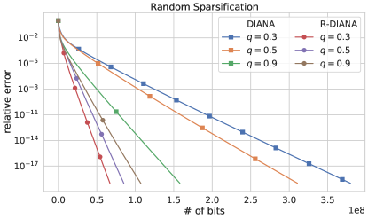
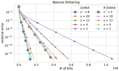
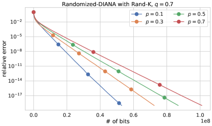
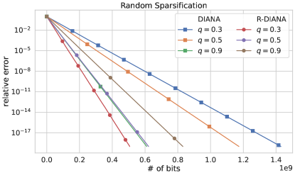
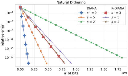
Figure 1: Comparison of DIANA and Randomized-DIANA. Left plot: methods equipped with Rand-K for different q𝑞q values. Right plot: selected results of a grid search for the ND parameter s𝑠s over {2,,20}220\{2,\dots,20\}.

The essence of this method is compression of the local workers’ iterates 𝒬i(xkγfi(xk))subscript𝒬𝑖superscript𝑥𝑘𝛾subscript𝑓𝑖superscript𝑥𝑘\mathcal{Q}_{i}\left(x^{k}-\gamma\nabla f_{i}(x^{k})\right), their aggregation on the master and convex combination with the previous model. Next we present established linear convergence up to a neighborhood introduced due to variance of compression operator (similarly to DCGD with fixed shifts Theorem 1).

Theorem 5 (GDCI).

Assume each fisubscript𝑓𝑖f_{i} is convex and Lisubscript𝐿𝑖L_{i}-smooth, and f𝑓f is L𝐿L-smooth and μ𝜇\mu-strongly convex. Let 𝒬i𝕌(ω)subscript𝒬𝑖𝕌𝜔\mathcal{Q}_{i}\in\mathbb{U}(\omega) be independent compression operators. If the step-sizes satisfy

η[Lμ+2ωn(Lmaxμ1)]1,γ1+2ηω/nη(L+2Lmaxω/n),formulae-sequence𝜂superscriptdelimited-[]𝐿𝜇2𝜔𝑛subscript𝐿𝜇11𝛾12𝜂𝜔𝑛𝜂𝐿2subscript𝐿𝜔𝑛\eta\leq\left[\frac{L}{\mu}+\frac{2\omega}{n}\left(\frac{L_{\max}}{\mu}-1\right)\right]^{-1},\gamma\leq\frac{1+2\eta\omega/n}{\eta\left(L+2L_{\max}\omega/n\right)},

then the iterates of the Distributed GDCI (13) satisfy

𝐄xkx2𝐄superscriptnormsuperscript𝑥𝑘superscript𝑥2\displaystyle\operatorname{\mathbf{E}}\left\|x^{k}-x^{\star}\right\|^{2} (1η)kx0x2absentsuperscript1𝜂𝑘superscriptnormsuperscript𝑥0superscript𝑥2\displaystyle\leq(1-\eta)^{k}\|x^{0}-x^{\star}\|^{2} (14)
+η2ωn1ni=1nxγfi(x)2.𝜂2𝜔𝑛1𝑛superscriptsubscript𝑖1𝑛superscriptnormsuperscript𝑥𝛾subscript𝑓𝑖superscript𝑥2\displaystyle\ \ +\eta\frac{2\omega}{n}\frac{1}{n}\sum_{i=1}^{n}\left\|x^{\star}-\gamma\nabla f_{i}(x^{\star})\right\|^{2}.

In the interpolation regime (fi(x)=0=xγfi(x)subscript𝑓𝑖superscript𝑥0superscript𝑥𝛾subscript𝑓𝑖superscript𝑥\nabla f_{i}(x^{\star})=0=x^{\star}-\gamma\nabla f_{i}(x^{\star}), for every i𝑖i) this result matches the complexity of DCGD with fixed shifts (7)

𝒪~(κ(1+ω/n))~𝒪𝜅1𝜔𝑛\tilde{\mathcal{O}}\left(\kappa\left(1+\omega/n\right)\right)

and improves over the original rate of GDCI by Chraibi et al. (2019) analyzed for fixed point problems and specialized for gradient mappings:

𝒪~(κmax{1,κω/n})𝒪~(κ2ω/n).greater-than-or-equivalent-to~𝒪𝜅1𝜅𝜔𝑛~𝒪superscript𝜅2𝜔𝑛\tilde{\mathcal{O}}\left(\kappa\max\left\{1,\kappa\omega/n\right\}\right)\gtrsim\tilde{\mathcal{O}}\left(\kappa^{2}\omega/n\right).

Due to space limitations, the results for Distributed Variance-Reduced Gradient Descent with Compressed Iterates (VR-GDCI), which eliminates the neighborhood in (14), along with detailed proofs of all stated theorems are presented in the Supplementary Material.
Refer to caption
Refer to caption
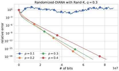
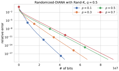
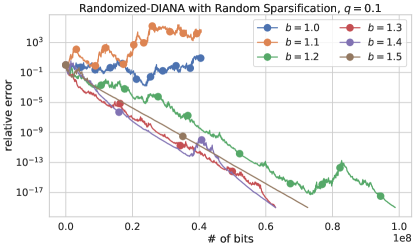
Figure 2: Study of the stability and performance of Rand-DIANA with varying parameters b𝑏b and p𝑝p.

4 EXPERIMENTS

In this section, we present some of the experimental results obtained. The remainder of the results (including real-world data and other models) are available in Section C of the Supplementary Material. To provide evidence that our theory translates into observable predictions, we focus on well-controlled settings that satisfy the assumptions in our work.

Consider a classical ridge-regression optimization problem

minxd[f(x)12Axy2+λ2x2],subscript𝑥superscript𝑑𝑓𝑥12superscriptnormA𝑥𝑦2𝜆2superscriptnorm𝑥2\min_{x\in\mathbb{R}^{d}}\left[f(x)\coloneqq\frac{1}{2}\|\mathrm{A}x-y\|^{2}+\frac{\lambda}{2}\|x\|^{2}\right],

where λ=1/m𝜆1𝑚\lambda=1/m and Am×d,ymformulae-sequenceAsuperscript𝑚𝑑𝑦superscript𝑚\mathrm{A}\in\mathbb{R}^{m\times d},y\in\mathbb{R}^{m} are generated using the Scikit-learn library (Pedregosa et al., 2011) method sklearn.datasets.make_regression with default parameters for m=100,d=80formulae-sequence𝑚100𝑑80m=100,d=80. The obtained data is uniformly, evenly, and randomly distributed among 10 workers. To compare selected algorithms, we evaluate the logarithm of a relative argument error log(xkx2/x0x2)superscriptnormsuperscript𝑥𝑘superscript𝑥2superscriptnormsuperscript𝑥0superscript𝑥2\log\left(\|x^{k}-x^{\star}\|^{2}/\|x^{0}-x^{\star}\|^{2}\right) on the vertical axis, while the horizontal axis presents the number of communicated bits needed to reach a certain error tolerance ε𝜀\varepsilon. The starting point x0dsuperscript𝑥0superscript𝑑x^{0}\in\mathbb{R}^{d} entries are sampled from the normal distribution 𝒩(0,10)𝒩010\mathcal{N}(0,10).

In our simulations we thoroughly examine the Rand-DIANA method, which is presented for the first time. Extensive studies of the methods with compressed iterates can be found in the works by Khaled and Richtárik (2019); Chraibi et al. (2019).

4.1 Randomized-DIANA vs DIANA

In the first set of experiments, we compare Rand-DIANA and DIANA with different compressors 𝒬isubscript𝒬𝑖\mathcal{Q}_{i} (𝒞i0subscript𝒞𝑖0\mathcal{C}_{i}\equiv 0) and varied operators’ parameters. The results obtained are summarized in Figure 1. The designation qk/d𝑞𝑘𝑑q\coloneqq k/d is used for the share of non-zeroed coordinates of the Random sparsification (Rand-K) operator, and s𝑠s corresponds to the number of levels for the Natural Dithering (ND) (Horváth et al., 2019a) compressor. The p𝑝p parameter of Rand-DIANA was set at 1/(ω+1)1𝜔11/(\omega+1) for every run.

The left plot in Figure 1 clearly shows that Rand-DIANA performs better than DIANA for every value of the Rand-K compressor parameter. It is worth noting that DIANA performs better at higher q𝑞q, while the opposite holds for Rand-DIANA.

From the right plot in Figure 1, one can see that DIANA with ND can be superior to Rand-DIANA for the optimized parameter ssuperscript𝑠s^{\star}. Nevertheless, Rand-DIANA is highly preferable for very aggressive compression (e.g., s=2𝑠2s=2).

In the next experimental setup, we more closely investigate the behavior of Rand-DIANA with respect to its parameters.

4.2 Randomized-DIANA Study

According to the formulation of Theorem 4, the constant M𝑀M has to be strictly greater than M2ω/(np)superscript𝑀2𝜔𝑛𝑝M^{\prime}\coloneqq 2\omega/(np). In the left plot of Figure 2, we show that the method becomes less stable and can even diverge for smaller values of M𝑀M (set to Mbsuperscript𝑀𝑏M^{\prime}\cdot b). However, too high M𝑀M (for b=1.5𝑏1.5b=1.5) can lead to an overall (stable) slowdown. We conclude that the condition imposed by theoretical analysis is indeed critical.

The right plot in Figure 2 examines how the parameter p𝑝p affects the convergence in a high compression regime (q=0.1𝑞0.1q=0.1). The method converges faster for smaller p𝑝p and can diverge above a certain threshold, similarly to the previous study of M𝑀M trade-off.

We did not conduct additional experiments to show the effect of combining unbiased compressors with biased counterparts, as the benefits of such an approach have already been clearly demonstrated by Horváth and Richtárik (2021) for distributed training of deep neural networks.

Acknowledgements.
We would like to thank the anonymous reviewers, Laurent Condat and Konstantin Mishchenko for their helpful comments and suggestions to improve the manuscript.

References

  • Albasyoni et al. (2020) Albasyoni A., Safaryan M., Condat L. and Richtárik P. Optimal gradient compression for distributed and federated learning. arXiv preprint arXiv:2010.03246, 2020.
  • Alistarh et al. (2017) Alistarh D., Grubic D., Li J., Tomioka R. and Vojnovic M. QSGD: Communication-efficient SGD via gradient quantization and encoding. volume 30. 2017.
  • Alistarh et al. (2018) Alistarh D., Hoefler T., Johansson M., Konstantinov N., Khirirat S. and Renggli C. The convergence of sparsified gradient methods. In Advances in Neural Information Processing Systems, pp. 5973–5983. 2018.
  • Basu et al. (2019) Basu D., Data D., Karakus C. and Diggavi S. Qsparse-local-SGD: Distributed SGD with quantization, sparsification and local computations. In Advances in Neural Information Processing Systems, pp. 14668–14679. 2019.
  • Bernstein et al. (2018) Bernstein J., Wang Y.X., Azizzadenesheli K. and Anandkumar A. signSGD: compressed optimisation for non-convex problems. In International Conference on Machine Learning. 2018.
  • Beznosikov et al. (2020) Beznosikov A., Horváth S., Richtárik P. and Safaryan M. On biased compression for distributed learning. arXiv preprint arXiv:2002.12410, 2020.
  • by: Peter Kairouz and McMahan (2021) by: Peter Kairouz E. and McMahan H.B. Advances and open problems in federated learning. Foundations and Trends® in Machine Learning, 14(1), 2021.
  • Chang and Lin (2011) Chang C.C. and Lin C.J. LIBSVM: A library for support vector machines. ACM Transactions on Intelligent Systems and Technology, 2:27:1, 2011. Software available at http://www.csie.ntu.edu.tw/~cjlin/libsvm.
  • Chraibi et al. (2019) Chraibi S., Khaled A., Kovalev D., Richtárik P., Salim A. and Takáč M. Distributed fixed point methods with compressed iterates. arXiv preprint arXiv:2102.07245, 2019.
  • Condat and Richtárik (2021) Condat L. and Richtárik P. MURANA: A generic framework for stochastic variance-reduced optimization. arXiv preprint arXiv:2106.03056, 2021.
  • Condat et al. (2022) Condat L., Yi K. and Richtárik P. EF-BV: A unified theory of error feedback and variance reduction mechanisms for biased and unbiased compression in distributed optimization. arXiv preprint arXiv:2205.04180, 2022.
  • Gandikota et al. (2021) Gandikota V., Kane D., Maity R.K. and Mazumdar A. vqSGD: Vector quantized stochastic gradient descent. In International Conference on Artificial Intelligence and Statistics, pp. 2197–2205. PMLR, 2021.
  • Goodall (1951) Goodall W. Television by pulse code modulation. Bell System Technical Journal, 30(1):33, 1951.
  • Gorbunov et al. (2020a) Gorbunov E., Hanzely F. and Richtárik P. A unified theory of SGD: Variance reduction, sampling, quantization and coordinate descent. In The 23rd International Conference on Artificial Intelligence and Statistics. 2020a.
  • Gorbunov et al. (2020b) Gorbunov E., Kovalev D., Makarenko D. and Richtárik P. Linearly converging error compensated SGD. volume 33, pp. 20889–20900. 2020b.
  • Goyal et al. (2018) Goyal P., Dollár P., Girshick R., Noordhuis P., Wesolowski L., Kyrola A., Tulloch A., Jia Y. and He K. Accurate, large minibatch SGD: Training ImageNet in 1 hour. arXiv preprint arXiv:1706.02677, 2018.
  • Horváth et al. (2019a) Horváth S., Ho C.Y., Horváth Ľ., Sahu A.N., Canini M. and Richtárik P. Natural compression for distributed deep learning. arXiv preprint arXiv:1905.10988, 2019a.
  • Horváth et al. (2019b) Horváth S., Kovalev D., Mishchenko K., Stich S. and Richtárik P. Stochastic distributed learning with gradient quantization and variance reduction. arXiv preprint arXiv:1904.05115, 2019b.
  • Horváth and Richtárik (2021) Horváth S. and Richtárik P. A better alternative to error feedback for communication-efficient distributed learning. In International Conference on Learning Representations. 2021.
  • Khaled and Richtárik (2019) Khaled A. and Richtárik P. Gradient descent with compressed iterates. NeurIPS 2019 Workshop on Federated Learning for Data Privacy and Confidentiality, 2019.
  • Khirirat et al. (2018) Khirirat S., Feyzmahdavian H.R. and Johansson M. Distributed learning with compressed gradients. arXiv preprint arXiv:1806.06573, 2018.
  • Konečný and Richtárik (2018) Konečný J. and Richtárik P. Randomized distributed mean estimation: Accuracy vs. communication. Frontiers in Applied Mathematics and Statistics, 4:62, 2018.
  • Konečný et al. (2016) Konečný J., McMahan H.B., Yu F.X., Richtárik P., Suresh A.T. and Bacon D. Federated learning: Strategies for improving communication efficiency. NIPS Private Multi-Party Machine Learning Workshop, 2016.
  • Kovalev et al. (2020) Kovalev D., Horváth S. and Richtárik P. Don’t jump through hoops and remove those loops: Svrg and katyusha are better without the outer loop. In Proceedings of the 31st International Conference on Algorithmic Learning Theory, volume 117 of Proceedings of Machine Learning Research, pp. 451–467. PMLR, 2020.
  • Li et al. (2020) Li Z., Kovalev D., Qian X. and Richtárik P. Acceleration for compressed gradient descent in distributed and federated optimization. Proceedings of the 37th International Conference on Machine Learning, 2020.
  • Luo et al. (2018) Luo L., Nelson J., Ceze L., Phanishayee A. and Krishnamurthy A. Parameter hub: a rack-scale parameter server for distributed deep neural network training. In Proceedings of the ACM Symposium on Cloud Computing, SoCC 2018, pp. 41–54. 2018.
  • McMahan et al. (2017) McMahan B., Moore E., Ramage D., Hampson S. and y Arcas B.A. Communication-efficient learning of deep networks from decentralized data. In Artificial intelligence and statistics, pp. 1273–1282. PMLR, 2017.
  • Mishchenko et al. (2019) Mishchenko K., Gorbunov E., Takáč M. and Richtárik P. Distributed learning with compressed gradient differences. arXiv preprint arXiv:1901.09269, 2019.
  • Mishchenko et al. (2022) Mishchenko K., Wang B., Kovalev D. and Richtárik P. IntSGD: Floatless compression of stochastic gradients. In International Conference on Learning Representations. 2022.
  • Nesterov (1983) Nesterov Y. A method of solving a convex programming problem with convergence rate o(1/k2)𝑜1superscript𝑘2o(1/k^{2}). Doklady Akademii Nauk USSR, 269(3):543, 1983.
  • Pedregosa et al. (2011) Pedregosa F., Varoquaux G., Gramfort A., Michel V., Thirion B., Grisel O., Blondel M., Prettenhofer P., Weiss R., Dubourg V., Vanderplas J., Passos A., Cournapeau D., Brucher M., Perrot M. and Duchesnay E. Scikit-learn: Machine learning in Python. Journal of Machine Learning Research, 12:2825, 2011.
  • Peng et al. (2019) Peng Y., Zhu Y., Chen Y., Bao Y., Yi B., Lan C., Wu C. and Guo C. A generic communication scheduler for distributed DNN training acceleration. In Proceedings of the 27th ACM Symposium on Operating Systems Principles, SOSP 2019, pp. 16–29. 2019.
  • Reisizadeh et al. (2020) Reisizadeh A., Mokhtari A., Hassani H., Jadbabaie A. and Pedarsani R. FedPAQ: A communication-efficient federated learning method with periodic averaging and quantization. In International Conference on Artificial Intelligence and Statistics, pp. 2021–2031. PMLR, 2020.
  • Roberts (1962) Roberts L. Picture coding using pseudo-random noise. IRE Transactions on Information Theory, 8(2):145, 1962.
  • Safaryan et al. (2021a) Safaryan M., Hanzely F. and Richtárik P. Smoothness matrices beat smoothness constants: better communication compression techniques for distributed optimization. Advances in Neural Information Processing Systems, 34, 2021a.
  • Safaryan et al. (2022) Safaryan M., Islamov R., Qian X. and Richtárik P. FedNL: Making newton-type methods applicable to federated learning. In International Conference on Machine Learning. 2022.
  • Safaryan and Richtárik (2021) Safaryan M. and Richtárik P. Stochastic sign descent methods: New algorithms and better theory. In International Conference on Machine Learning, pp. 9224–9234. PMLR, 2021.
  • Safaryan et al. (2021b) Safaryan M., Shulgin E. and Richtárik P. Uncertainty principle for communication compression in distributed and federated learning and the search for an optimal compressor. Information and Inference: A Journal of the IMA, 2021b.
  • Sapio et al. (2021) Sapio A., Canini M., Ho C., Nelson J., Kalnis P., Kim C., Krishnamurthy A., Moshref M., Ports D.R.K. and Richtárik P. Scaling distributed machine learning with in-network aggregation. In 18th USENIX Symposium on Networked Systems Design and Implementation, NSDI 2021, April 12-14, pp. 785–808. USENIX Association, 2021.
  • Seide et al. (2014) Seide F., Fu H., Droppo J., Li G. and Yu D. 1-bit stochastic gradient descent and its application to data-parallel distributed training of speech dnns. In Fifteenth Annual Conference of the International Speech Communication Association. 2014.
  • Stich et al. (2018) Stich S.U., Cordonnier J.B. and Jaggi M. Sparsified SGD with memory. In Advances in Neural Information Processing Systems, pp. 4447–4458. 2018.
  • Stich and Karimireddy (2020) Stich S.U. and Karimireddy S.P. The error-feedback framework: SGD with delayed gradients. Journal of Machine Learning Research, 21(237):1, 2020.
  • Vogels et al. (2020) Vogels T., Karimireddy S.P. and Jaggi M. Practical low-rank communication compression in decentralized deep learning. volume 33, pp. 14171–14181. 2020.
  • Wang et al. (2018) Wang H., Sievert S., Liu S., Charles Z., Papailiopoulos D. and Wright S. Atomo: Communication-efficient learning via atomic sparsification. In Advances in Neural Information Processing Systems, volume 31. 2018.
  • Wangni et al. (2018) Wangni J., Wang J., Liu J. and Zhang T. Gradient sparsification for communication-efficient distributed optimization. In Advances in Neural Information Processing Systems, pp. 1299–1309. 2018.
  • Wen et al. (2017) Wen W., Xu C., Yan F., Wu C., Wang Y., Chen Y. and Li H. Terngrad: Ternary gradients to reduce communication in distributed deep learning. In Advances in Neural Information Processing Systems, pp. 1509–1519. 2017.
  • Xu et al. (2020) Xu H., Ho C.Y., Abdelmoniem A.M., Dutta A., Bergou E.H., Karatsenidis K., Canini M. and Kalnis P. Compressed communication for distributed deep learning: Survey and quantitative evaluation. Technical report, 2020.

Supplementary Material

Appendix A BASIC FACTS

Bregman Divergence associated with a continuously differentiable, strictly convex function f:dd:𝑓superscript𝑑superscript𝑑f:\mathbb{R}^{d}\to\mathbb{R}^{d} is defined as

Df(x,y)f(x)f(y)f(y),xy.subscript𝐷𝑓𝑥𝑦𝑓𝑥𝑓𝑦𝑓𝑦𝑥𝑦D_{f}(x,y)\coloneqq f(x)-f(y)-\langle\nabla f(y),x-y\rangle.
Bregman Divergence and Strong Convexity Inequality:
f(x)f(y),xyDf(x,y)+μ2xy2.𝑓𝑥𝑓𝑦𝑥𝑦subscript𝐷𝑓𝑥𝑦𝜇2superscriptnorm𝑥𝑦2\langle\nabla f(x)-\nabla f(y),x-y\rangle\geq D_{f}(x,y)+\frac{\mu}{2}\|x-y\|^{2}. (15)
Bregman Divergence and L𝐿L-smoothness Inequality:
f(x)f(y)22LDf(x,y).superscriptnorm𝑓𝑥𝑓𝑦22𝐿subscript𝐷𝑓𝑥𝑦\|\nabla f(x)-\nabla f(y)\|^{2}\leq 2LD_{f}(x,y). (16)
Basic Inequalities.

For all vectors a,bd𝑎𝑏superscript𝑑a,b\in\mathbb{R}^{d} and random vector Xd𝑋superscript𝑑X\in\mathbb{R}^{d}:

a+b22a2+2b2,superscriptnorm𝑎𝑏22superscriptnorm𝑎22superscriptnorm𝑏2\|a+b\|^{2}\leq 2\|a\|^{2}+2\|b\|^{2}, (17)
2a,b=a2+b2ab2,2𝑎𝑏superscriptnorm𝑎2superscriptnorm𝑏2superscriptnorm𝑎𝑏22\langle a,b\rangle=\|a\|^{2}+\|b\|^{2}-\|a-b\|^{2}, (18)
𝐄Xa2=𝐄X𝐄X2+𝐄Xa2.𝐄superscriptnorm𝑋𝑎2𝐄superscriptnorm𝑋𝐄𝑋2superscriptnorm𝐄𝑋𝑎2\operatorname{\mathbf{E}}\|X-a\|^{2}=\operatorname{\mathbf{E}}\|X-\operatorname{\mathbf{E}}X\|^{2}+\|\operatorname{\mathbf{E}}X-a\|^{2}. (19)

Appendix B PROOFS

For brevity, we can use the notation 𝐄x2𝐄superscriptnorm𝑥2\operatorname{\mathbf{E}}\left\|x\right\|^{2} instead of 𝐄[x2]𝐄delimited-[]superscriptnorm𝑥2{\mathbf{E}}\left[\left\|x\right\|^{2}\right].

B.1 Shifted Compression

B.1.1 Proof of Lemma 1

Proof.

For the proof, we need to show unbiasedness and the (shifted) bounded variance property for operator 𝒬v+𝒬h(xv)𝒬𝑣subscript𝒬𝑥𝑣\mathcal{Q}\coloneqq v+\mathcal{Q}_{h}(x-v) with 𝒬h𝕌(ω;h)subscript𝒬𝕌𝜔\mathcal{Q}_{h}\in\mathbb{U}(\omega;h).
(a) Unbiasdeness:

𝐄𝒬(x)=𝐄[v+𝒬h(xv)]=v+𝐄𝒬h(xv)=v+(xv)=x.𝐄𝒬𝑥𝐄delimited-[]𝑣subscript𝒬𝑥𝑣𝑣𝐄subscript𝒬𝑥𝑣𝑣𝑥𝑣𝑥\operatorname{\mathbf{E}}\mathcal{Q}(x)={\mathbf{E}}\left[v+\mathcal{Q}_{h}(x-v)\right]=v+\operatorname{\mathbf{E}}\mathcal{Q}_{h}(x-v)=v+(x-v)=x.

(b) Variance:

𝐄𝒬(x)x2𝐄superscriptnorm𝒬𝑥𝑥2\displaystyle\operatorname{\mathbf{E}}\left\|\mathcal{Q}(x)-x\right\|^{2} =𝐄v+𝒬h(xv)x2absent𝐄superscriptnorm𝑣subscript𝒬𝑥𝑣𝑥2\displaystyle=\operatorname{\mathbf{E}}\left\|v+\mathcal{Q}_{h}(x-v)-x\right\|^{2}
=𝐄𝒬h(xv)(xv)2absent𝐄superscriptnormsubscript𝒬𝑥𝑣𝑥𝑣2\displaystyle=\operatorname{\mathbf{E}}\left\|\mathcal{Q}_{h}(x-v)-(x-v)\right\|^{2}
ωx(v+h)2,absent𝜔superscriptnorm𝑥𝑣2\displaystyle\leq\omega\left\|x-(v+h)\right\|^{2},

where the last inequality is due to the Shifted Compressor Definition 3. ∎

B.1.2 Compression of the Iterates

Lemma 2.

Let 𝒬𝕌(ω)𝒬𝕌𝜔\mathcal{Q}\in\mathbb{U}(\omega), then for

𝒬^(z)t𝒬(zt),t0,formulae-sequence^𝒬𝑧𝑡𝒬𝑧𝑡𝑡0\hat{\mathcal{Q}}(z)\coloneqq-t\cdot\mathcal{Q}\left(-\frac{z}{t}\right),\qquad t\neq 0, (20)

we have 𝒬^(z)𝕌(ω)^𝒬𝑧𝕌𝜔\hat{\mathcal{Q}}(z)\in\mathbb{U}(\omega).

Proof.

We consequentially show the unbiasedness (1) and bounded variance (2) properties according to Definition 2

1)𝐄𝒬^(z)=t𝐄𝒬(zt)=t(zt)=z;\displaystyle 1)\operatorname{\mathbf{E}}\hat{\mathcal{Q}}(z)=-t\cdot\operatorname{\mathbf{E}}\mathcal{Q}\left(-\frac{z}{t}\right)=-t\cdot\left(-\frac{z}{t}\right)=z;
2)𝐄𝒬^(z)2=𝐄t𝒬(zt)2=t2𝐄𝒬(zt)2t2(ω+1)zt2=(ω+1)z2.\displaystyle 2)\operatorname{\mathbf{E}}\left\|\hat{\mathcal{Q}}(z)\right\|^{2}=\operatorname{\mathbf{E}}\left\|-t\cdot\mathcal{Q}\left(-\frac{z}{t}\right)\right\|^{2}=t^{2}\operatorname{\mathbf{E}}\left\|\mathcal{Q}\left(-\frac{z}{t}\right)\right\|^{2}\leq t^{2}(\omega+1)\left\|-\frac{z}{t}\right\|^{2}=(\omega+1)\|z\|^{2}.

Now, we prove that the shifted compressor 𝒬~(z)1γ[x𝒬(xγz)]~𝒬𝑧1𝛾delimited-[]𝑥𝒬𝑥𝛾𝑧\tilde{\mathcal{Q}}(z)\coloneqq\frac{1}{\gamma}\left[x-\mathcal{Q}(x-\gamma z)\right], obtained from (20) by the procedure described in Section 3.3, belongs to class 𝕌(ω;x/γ)𝕌𝜔𝑥𝛾\mathbb{U}\left(\omega;x/\gamma\right) for 𝒬𝕌(ω)𝒬𝕌𝜔\mathcal{Q}\in\mathbb{U}(\omega).

Proof.

1) Unbiasedness follows from 𝐄𝒬(x)=x𝐄𝒬𝑥𝑥\operatorname{\mathbf{E}}\mathcal{Q}(x)=x.

2) Computation of the variance:

𝐄𝒬~(z)2𝐄superscriptnorm~𝒬𝑧2\displaystyle\operatorname{\mathbf{E}}\left\|\tilde{\mathcal{Q}}(z)\right\|^{2} =𝐄1γ[x𝒬(xγz)]2absent𝐄superscriptnorm1𝛾delimited-[]𝑥𝒬𝑥𝛾𝑧2\displaystyle=\operatorname{\mathbf{E}}\left\|\frac{1}{\gamma}\left[x-\mathcal{Q}(x-\gamma z)\right]\right\|^{2}
=1γ2𝐄x𝒬(xγz)2absent1superscript𝛾2𝐄superscriptnorm𝑥𝒬𝑥𝛾𝑧2\displaystyle=\frac{1}{\gamma^{2}}\operatorname{\mathbf{E}}\left\|x-\mathcal{Q}(x-\gamma z)\right\|^{2}
=1γ2𝐄xγz𝒬(xγz)+γz2absent1superscript𝛾2𝐄superscriptnorm𝑥𝛾𝑧𝒬𝑥𝛾𝑧𝛾𝑧2\displaystyle=\frac{1}{\gamma^{2}}\operatorname{\mathbf{E}}\left\|x-\gamma z-\mathcal{Q}(x-\gamma z)+\gamma z\right\|^{2}
=1γ2[𝐄xγz𝒬(xγz)2+γz2]absent1superscript𝛾2delimited-[]𝐄superscriptnorm𝑥𝛾𝑧𝒬𝑥𝛾𝑧2superscriptnorm𝛾𝑧2\displaystyle=\frac{1}{\gamma^{2}}\left[\operatorname{\mathbf{E}}\left\|x-\gamma z-\mathcal{Q}(x-\gamma z)\right\|^{2}+\|\gamma z\|^{2}\right]
21γ2[ωxγz2+γz2]superscript2absent1superscript𝛾2delimited-[]𝜔superscriptnorm𝑥𝛾𝑧2superscriptnorm𝛾𝑧2\displaystyle\stackrel{{\scriptstyle\ref{def:unbiased_compressor}}}{{\leq}}\frac{1}{\gamma^{2}}\left[\omega\left\|x-\gamma z\right\|^{2}+\|\gamma z\|^{2}\right]
=ωxγz2+z2,absent𝜔superscriptnorm𝑥𝛾𝑧2superscriptnorm𝑧2\displaystyle=\omega\left\|\frac{x}{\gamma}-z\right\|^{2}+\|z\|^{2},

which implies

𝐄𝒬~(z)z2ωzxγ2.𝐄superscriptnorm~𝒬𝑧𝑧2𝜔superscriptnorm𝑧𝑥𝛾2\operatorname{\mathbf{E}}\left\|\tilde{\mathcal{Q}}(z)-z\right\|^{2}\leq\omega\left\|z-\frac{x}{\gamma}\right\|^{2}.

B.1.3 Induced Compressor

Definition 4 (Induced Compression Operator (Horváth and Richtárik, 2021)).

For 𝒞𝔹(δ)𝒞𝔹𝛿\mathcal{C}\in\mathbb{B}(\delta), choose 𝒬𝕌(ω)𝒬𝕌𝜔\mathcal{Q}\in\mathbb{U}(\omega) and define the induced compressor via

𝒞ind(x)𝒞(x)+𝒬(x𝒞(x)).subscript𝒞ind𝑥𝒞𝑥𝒬𝑥𝒞𝑥\mathcal{C}_{\mathrm{ind}}(x)\coloneqq\mathcal{C}(x)+\mathcal{Q}(x-\mathcal{C}(x)). (21)
Lemma 3.

The induced operator satisfies 𝒞ind𝕌(ω~)subscript𝒞ind𝕌~𝜔\mathcal{C}_{\mathrm{ind}}\in\mathbb{U}(\tilde{\omega}) for

ω~=ω(1δ).~𝜔𝜔1𝛿\tilde{\omega}=\omega(1-\delta). (22)
Proof.
𝐄𝒞ind(x)x2𝐄superscriptnormsubscript𝒞ind𝑥𝑥2\displaystyle\operatorname{\mathbf{E}}\|\mathcal{C}_{\mathrm{ind}}(x)-x\|^{2} =(21)𝐄𝒬(x𝒞(x))(x𝒞(x))2superscriptitalic-(21italic-)absent𝐄superscriptnorm𝒬𝑥𝒞𝑥𝑥𝒞𝑥2\displaystyle\stackrel{{\scriptstyle\eqref{eq:induced_compressor}}}{{=}}\operatorname{\mathbf{E}}\|\mathcal{Q}(x-\mathcal{C}(x))-(x-\mathcal{C}(x))\|^{2}
2ω𝐄x𝒞(x)2superscript2absent𝜔𝐄superscriptnorm𝑥𝒞𝑥2\displaystyle\stackrel{{\scriptstyle\ref{def:unbiased_compressor}}}{{\leq}}\omega\operatorname{\mathbf{E}}\|x-\mathcal{C}(x)\|^{2}
1ω(1δ)x2superscript1absent𝜔1𝛿superscriptnorm𝑥2\displaystyle\stackrel{{\scriptstyle\ref{def:general_compressor}}}{{\leq}}\omega(1-\delta)\|x\|^{2}
=ω~x2.absent~𝜔superscriptnorm𝑥2\displaystyle=\tilde{\omega}\|x\|^{2}.

B.2 Proof of Theorem 1 (DCGD-SHIFT)

According to Algorithm 1, the gradient estimator always has the following form

gh(x)=1ni=1nghi(x)=1ni=1n[hi+𝒬i(fi(x)hi)].subscript𝑔𝑥1𝑛superscriptsubscript𝑖1𝑛subscript𝑔subscript𝑖𝑥1𝑛superscriptsubscript𝑖1𝑛delimited-[]subscript𝑖subscript𝒬𝑖subscript𝑓𝑖𝑥subscript𝑖g_{h}(x)=\frac{1}{n}\sum_{i=1}^{n}g_{h_{i}}(x)=\frac{1}{n}\sum_{i=1}^{n}\left[h_{i}+\mathcal{Q}_{i}\left(\nabla f_{i}(x)-h_{i}\right)\right]. (23)

The obvious unbiasedness (as 𝒬i𝕌(ωi)subscript𝒬𝑖𝕌subscript𝜔𝑖\mathcal{Q}_{i}\in\mathbb{U}(\omega_{i})) of this estimator for any hisubscript𝑖h_{i} will be used in all further proofs.

Decomposition due to (19)

𝐄gh(xk)f(x)2=𝐄gh(xk)f(xk)2+f(xk)f(x)2.𝐄superscriptnormsubscript𝑔superscript𝑥𝑘𝑓superscript𝑥2𝐄superscriptnormsubscript𝑔superscript𝑥𝑘𝑓superscript𝑥𝑘2superscriptnorm𝑓superscript𝑥𝑘𝑓superscript𝑥2\operatorname{\mathbf{E}}\left\|g_{h}(x^{k})-\nabla f(x^{\star})\right\|^{2}=\operatorname{\mathbf{E}}\left\|g_{h}(x^{k})-\nabla f(x^{k})\right\|^{2}+\left\|\nabla f(x^{k})-\nabla f(x^{\star})\right\|^{2}. (24)

Next, we upper-bound the first term from (24).

Expectation conditional on xksuperscript𝑥𝑘x^{k} and h=(h1,,hn)subscript1subscript𝑛h=(h_{1},\dots,h_{n}) for brevity

𝐄gh(xk)f(xk)2𝐄superscriptnormsubscript𝑔superscript𝑥𝑘𝑓superscript𝑥𝑘2\displaystyle\operatorname{\mathbf{E}}\left\|g_{h}(x^{k})-\nabla f(x^{k})\right\|^{2} =𝐄gh(xk)f(xk)2absent𝐄superscriptnormsubscript𝑔superscript𝑥𝑘𝑓superscript𝑥𝑘2\displaystyle=\operatorname{\mathbf{E}}\left\|g_{h}(x^{k})-\nabla f(x^{k})\right\|^{2}
=(23)𝐄1ni=1n𝒬i(fi(xk)hi)+hifi(xk)bik2superscriptitalic-(23italic-)absent𝐄superscriptnorm1𝑛superscriptsubscript𝑖1𝑛subscriptsubscript𝒬𝑖subscript𝑓𝑖superscript𝑥𝑘subscript𝑖subscript𝑖subscript𝑓𝑖superscript𝑥𝑘superscriptsubscript𝑏𝑖𝑘2\displaystyle\stackrel{{\scriptstyle\eqref{eq:grad_estimator}}}{{=}}\operatorname{\mathbf{E}}\Bigg{\|}\frac{1}{n}\sum_{i=1}^{n}\underbracket{\mathcal{Q}_{i}\left(\nabla f_{i}(x^{k})-h_{i}\right)+h_{i}-\nabla f_{i}(x^{k})}_{b_{i}^{k}}\Bigg{\|}^{2}
=1n2𝐄[i=1nbik2+ijbik,bjk]absent1superscript𝑛2𝐄delimited-[]superscriptsubscript𝑖1𝑛superscriptnormsuperscriptsubscript𝑏𝑖𝑘2subscript𝑖𝑗superscriptsubscript𝑏𝑖𝑘superscriptsubscript𝑏𝑗𝑘\displaystyle=\frac{1}{n^{2}}{\mathbf{E}}\left[\sum_{i=1}^{n}\|b_{i}^{k}\|^{2}+\sum_{i\neq j}\langle b_{i}^{k},b_{j}^{k}\rangle\right]
=1n2i=1n𝐄bik2+1n2ij𝐄bik,𝐄bjk=0(𝐄𝒬i(x)=x)absent1superscript𝑛2superscriptsubscript𝑖1𝑛𝐄superscriptnormsuperscriptsubscript𝑏𝑖𝑘21superscript𝑛2subscript𝑖𝑗subscript𝐄superscriptsubscript𝑏𝑖𝑘𝐄superscriptsubscript𝑏𝑗𝑘absent0𝐄subscript𝒬𝑖𝑥𝑥\displaystyle=\frac{1}{n^{2}}\sum_{i=1}^{n}\operatorname{\mathbf{E}}\|b_{i}^{k}\|^{2}+\frac{1}{n^{2}}\sum_{i\neq j}\underbracket{\langle\operatorname{\mathbf{E}}b_{i}^{k},\operatorname{\mathbf{E}}b_{j}^{k}\rangle}_{=0\ (\operatorname{\mathbf{E}}\mathcal{Q}_{i}(x)=x)}
=1n2i=1n𝐄𝒬i(fi(xk)hi)+hifi(xk)2absent1superscript𝑛2superscriptsubscript𝑖1𝑛𝐄superscriptnormsubscript𝒬𝑖subscript𝑓𝑖superscript𝑥𝑘subscript𝑖subscript𝑖subscript𝑓𝑖superscript𝑥𝑘2\displaystyle=\frac{1}{n^{2}}\sum_{i=1}^{n}\operatorname{\mathbf{E}}\|\mathcal{Q}_{i}\left(\nabla f_{i}(x^{k})-h_{i}\right)+h_{i}-\nabla f_{i}(x^{k})\|^{2}
21n2i=1nωifi(xk)hi2superscript2absent1superscript𝑛2superscriptsubscript𝑖1𝑛subscript𝜔𝑖superscriptnormsubscript𝑓𝑖superscript𝑥𝑘subscript𝑖2\displaystyle\stackrel{{\scriptstyle\ref{def:unbiased_compressor}}}{{\leq}}\frac{1}{n^{2}}\sum_{i=1}^{n}\omega_{i}\|\nabla f_{i}(x^{k})-h_{i}\|^{2}
=1n2i=1nωifi(xk)fi(x)(hifi(x))2absent1superscript𝑛2superscriptsubscript𝑖1𝑛subscript𝜔𝑖superscriptnormsubscript𝑓𝑖superscript𝑥𝑘subscript𝑓𝑖superscript𝑥subscript𝑖subscript𝑓𝑖superscript𝑥2\displaystyle=\frac{1}{n^{2}}\sum_{i=1}^{n}\omega_{i}\|\nabla f_{i}(x^{k})-\nabla f_{i}(x^{\star})-\left(h_{i}-\nabla f_{i}(x^{\star})\right)\|^{2}
(17)2n2i=1nωi[fi(xk)fi(x)2+hifi(x)2]superscriptitalic-(17italic-)absent2superscript𝑛2superscriptsubscript𝑖1𝑛subscript𝜔𝑖delimited-[]superscriptnormsubscript𝑓𝑖superscript𝑥𝑘subscript𝑓𝑖superscript𝑥2superscriptnormsubscript𝑖subscript𝑓𝑖superscript𝑥2\displaystyle\stackrel{{\scriptstyle\eqref{eq:triangle}}}{{\leq}}\frac{2}{n^{2}}\sum_{i=1}^{n}\omega_{i}\left[\left\|\nabla f_{i}(x^{k})-\nabla f_{i}(x^{\star})\right\|^{2}+\left\|h_{i}-\nabla f_{i}(x^{\star})\right\|^{2}\right]
(16)2n2i=1nωi2LiDfi(xk,x)+2n2i=1nωihifi(x)2superscriptitalic-(16italic-)absent2superscript𝑛2superscriptsubscript𝑖1𝑛subscript𝜔𝑖2subscript𝐿𝑖subscript𝐷subscript𝑓𝑖superscript𝑥𝑘superscript𝑥2superscript𝑛2superscriptsubscript𝑖1𝑛subscript𝜔𝑖superscriptnormsubscript𝑖subscript𝑓𝑖superscript𝑥2\displaystyle\stackrel{{\scriptstyle\eqref{eq:smooth_bregman}}}{{\leq}}\frac{2}{n^{2}}\sum_{i=1}^{n}\omega_{i}\cdot 2L_{i}D_{f_{i}}(x^{k},x^{\star})+\frac{2}{n^{2}}\sum_{i=1}^{n}\omega_{i}\left\|h_{i}-\nabla f_{i}(x^{\star})\right\|^{2}
4nmax(ωiLi)1ni=1nDfi(xk,x)+2n2i=1nωihifi(x)2absent4𝑛subscript𝜔𝑖subscript𝐿𝑖1𝑛superscriptsubscript𝑖1𝑛subscript𝐷subscript𝑓𝑖superscript𝑥𝑘superscript𝑥2superscript𝑛2superscriptsubscript𝑖1𝑛subscript𝜔𝑖superscriptnormsubscript𝑖subscript𝑓𝑖superscript𝑥2\displaystyle\leq\frac{4}{n}\max\left(\omega_{i}L_{i}\right)\frac{1}{n}\sum_{i=1}^{n}D_{f_{i}}(x^{k},x^{\star})+\frac{2}{n^{2}}\sum_{i=1}^{n}\omega_{i}\left\|h_{i}-\nabla f_{i}(x^{\star})\right\|^{2}
4nmax(ωiLi)Df(xk,x)+2n2i=1nωihifi(x)2.absent4𝑛subscript𝜔𝑖subscript𝐿𝑖subscript𝐷𝑓superscript𝑥𝑘superscript𝑥2superscript𝑛2superscriptsubscript𝑖1𝑛subscript𝜔𝑖superscriptnormsubscript𝑖subscript𝑓𝑖superscript𝑥2\displaystyle\leq\frac{4}{n}\max\left(\omega_{i}L_{i}\right)D_{f}(x^{k},x^{\star})+\frac{2}{n^{2}}\sum_{i=1}^{n}\omega_{i}\left\|h_{i}-\nabla f_{i}(x^{\star})\right\|^{2}.

Combined with (24), we obtain

𝐄[gh(xk)f(x)2xk,h]2[2nmax(ωiLi)+L]Df(xk,x)+2n2i=1nωihifi(x)2𝐄delimited-[]conditionalsuperscriptnormsubscript𝑔superscript𝑥𝑘𝑓superscript𝑥2superscript𝑥𝑘2delimited-[]2𝑛subscript𝜔𝑖subscript𝐿𝑖𝐿subscript𝐷𝑓superscript𝑥𝑘superscript𝑥2superscript𝑛2superscriptsubscript𝑖1𝑛subscript𝜔𝑖superscriptnormsubscript𝑖subscript𝑓𝑖superscript𝑥2{\mathbf{E}}\left[\left\|g_{h}(x^{k})-\nabla f(x^{\star})\right\|^{2}\mid x^{k},h\right]\leq 2\left[\frac{2}{n}\max\left(\omega_{i}L_{i}\right)+L\right]D_{f}(x^{k},x^{\star})+\frac{2}{n^{2}}\sum_{i=1}^{n}\omega_{i}\left\|h_{i}-\nabla f_{i}(x^{\star})\right\|^{2}

Now from Gorbunov et al. (2020a, Theorem 4.1), we obtain the statement of Theorem 3.

B.3 Proof of Theorem 2 (DCGD-STAR)

The Distributed Compressed Gradient Descent with optimal Shift is determined by the update

hik=hi+𝒞i(fi(xk)hi),superscriptsubscript𝑖𝑘superscriptsubscript𝑖subscript𝒞𝑖subscript𝑓𝑖superscript𝑥𝑘superscriptsubscript𝑖h_{i}^{k}=h_{i}^{\star}+\mathcal{C}_{i}(\nabla f_{i}(x^{k})-h_{i}^{\star}),

where hi=fi(x)superscriptsubscript𝑖subscript𝑓𝑖superscript𝑥h_{i}^{\star}=\nabla f_{i}(x^{\star}).

Proof.

First, we compute the variance of the estimator.

We use expectation conditional on xksuperscript𝑥𝑘x^{k} and hk=(h1k,,hnk)superscript𝑘subscriptsuperscript𝑘1subscriptsuperscript𝑘𝑛h^{k}=(h^{k}_{1},\dots,h^{k}_{n}), for brevity

𝐕𝐚𝐫[gk]𝐕𝐚𝐫superscript𝑔𝑘\displaystyle\operatorname{{\bf Var}}[g^{k}] =𝐄gk𝐄[gk]2absent𝐄superscriptnormsuperscript𝑔𝑘𝐄delimited-[]superscript𝑔𝑘2\displaystyle=\operatorname{\mathbf{E}}\left\|g^{k}-{\mathbf{E}}\left[g^{k}\right]\right\|^{2} (25)
=𝐄1ni=1n𝒬i(fi(xk)hik)+hikf(xk)2absent𝐄superscriptnorm1𝑛superscriptsubscript𝑖1𝑛subscript𝒬𝑖subscript𝑓𝑖superscript𝑥𝑘superscriptsubscript𝑖𝑘superscriptsubscript𝑖𝑘𝑓superscript𝑥𝑘2\displaystyle=\operatorname{\mathbf{E}}\Bigg{\|}\frac{1}{n}\sum_{i=1}^{n}\mathcal{Q}_{i}\left(\nabla f_{i}(x^{k})-h_{i}^{k}\right)+h_{i}^{k}-\nabla f(x^{k})\Bigg{\|}^{2}
=𝐄1ni=1n[𝒬i(fi(xk)hik)+hikfi(xk)]2absent𝐄superscriptnorm1𝑛superscriptsubscript𝑖1𝑛delimited-[]subscript𝒬𝑖subscript𝑓𝑖superscript𝑥𝑘superscriptsubscript𝑖𝑘superscriptsubscript𝑖𝑘subscript𝑓𝑖superscript𝑥𝑘2\displaystyle=\operatorname{\mathbf{E}}\Bigg{\|}\frac{1}{n}\sum_{i=1}^{n}\left[\mathcal{Q}_{i}\left(\nabla f_{i}(x^{k})-h_{i}^{k}\right)+h_{i}^{k}-\nabla f_{i}(x^{k})\right]\Bigg{\|}^{2}
=1n2i=1n𝐄𝒬i(fi(xk)hik)+hikfi(xk)2absent1superscript𝑛2superscriptsubscript𝑖1𝑛𝐄superscriptnormsubscript𝒬𝑖subscript𝑓𝑖superscript𝑥𝑘superscriptsubscript𝑖𝑘superscriptsubscript𝑖𝑘subscript𝑓𝑖superscript𝑥𝑘2\displaystyle=\frac{1}{n^{2}}\sum_{i=1}^{n}\operatorname{\mathbf{E}}\|\mathcal{Q}_{i}\left(\nabla f_{i}(x^{k})-h_{i}^{k}\right)+h_{i}^{k}-\nabla f_{i}(x^{k})\|^{2}
21n2i=1nωi𝐄fi(xk)hik2superscript2absent1superscript𝑛2superscriptsubscript𝑖1𝑛subscript𝜔𝑖𝐄superscriptnormsubscript𝑓𝑖superscript𝑥𝑘superscriptsubscript𝑖𝑘2\displaystyle\stackrel{{\scriptstyle\ref{def:unbiased_compressor}}}{{\leq}}\frac{1}{n^{2}}\sum_{i=1}^{n}\omega_{i}\operatorname{\mathbf{E}}\|\nabla f_{i}(x^{k})-h_{i}^{k}\|^{2}
=1n2i=1nωi𝐄fi(xk)hi𝒞i(fi(xk)hi)2absent1superscript𝑛2superscriptsubscript𝑖1𝑛subscript𝜔𝑖𝐄superscriptnormsubscript𝑓𝑖superscript𝑥𝑘superscriptsubscript𝑖subscript𝒞𝑖subscript𝑓𝑖superscript𝑥𝑘superscriptsubscript𝑖2\displaystyle=\frac{1}{n^{2}}\sum_{i=1}^{n}\omega_{i}\operatorname{\mathbf{E}}\|\nabla f_{i}(x^{k})-h_{i}^{\star}-\mathcal{C}_{i}\left(\nabla f_{i}(x^{k})-h_{i}^{\star}\right)\|^{2}
11n2i=1nωi(1δi)fi(xk)fi(x)2superscript1absent1superscript𝑛2superscriptsubscript𝑖1𝑛subscript𝜔𝑖1subscript𝛿𝑖superscriptnormsubscript𝑓𝑖superscript𝑥𝑘subscript𝑓𝑖superscript𝑥2\displaystyle\stackrel{{\scriptstyle\ref{def:general_compressor}}}{{\leq}}\frac{1}{n^{2}}\sum_{i=1}^{n}\omega_{i}(1-\delta_{i})\|\nabla f_{i}(x^{k})-\nabla f_{i}(x^{\star})\|^{2}
(16)1n2i=1nωi(1δi)2LiDfi(xk,x)superscriptitalic-(16italic-)absent1superscript𝑛2superscriptsubscript𝑖1𝑛subscript𝜔𝑖1subscript𝛿𝑖2subscript𝐿𝑖subscript𝐷subscript𝑓𝑖superscript𝑥𝑘superscript𝑥\displaystyle\stackrel{{\scriptstyle\eqref{eq:smooth_bregman}}}{{\leq}}\frac{1}{n^{2}}\sum_{i=1}^{n}\omega_{i}(1-\delta_{i})\cdot 2L_{i}D_{f_{i}}(x^{k},x^{\star})
2nmax{ωi(1δi)Li}1ni=1nDfi(xk,x)absent2𝑛subscript𝜔𝑖1subscript𝛿𝑖subscript𝐿𝑖1𝑛superscriptsubscript𝑖1𝑛subscript𝐷subscript𝑓𝑖superscript𝑥𝑘superscript𝑥\displaystyle\leq\frac{2}{n}\max\{\omega_{i}(1-\delta_{i})L_{i}\}\frac{1}{n}\sum_{i=1}^{n}D_{f_{i}}(x^{k},x^{\star})
2nmax{ωi(1δi)Li}Df(xk,x).absent2𝑛subscript𝜔𝑖1subscript𝛿𝑖subscript𝐿𝑖subscript𝐷𝑓superscript𝑥𝑘superscript𝑥\displaystyle\leq\frac{2}{n}\max\{\omega_{i}(1-\delta_{i})L_{i}\}D_{f}(x^{k},x^{\star}).

Now we can move to the convergence proof. Expectation conditional on xksuperscript𝑥𝑘x^{k} and hksuperscript𝑘h^{k}:

𝐄rk+12𝐄superscriptnormsuperscript𝑟𝑘12\displaystyle\operatorname{\mathbf{E}}\|r^{k+1}\|^{2} =𝐄xk+1x2absent𝐄superscriptnormsuperscript𝑥𝑘1superscript𝑥2\displaystyle=\operatorname{\mathbf{E}}\|x^{k+1}-x^{\star}\|^{2}
=𝐄xkγgk(xγf(x))2absent𝐄superscriptnormsuperscript𝑥𝑘𝛾superscript𝑔𝑘superscript𝑥𝛾𝑓superscript𝑥2\displaystyle=\operatorname{\mathbf{E}}\|x^{k}-\gamma g^{k}-(x^{\star}-\gamma\nabla f(x^{\star}))\|^{2}
=𝐄xkxγ(gkf(x))2absent𝐄superscriptnormsuperscript𝑥𝑘superscript𝑥𝛾superscript𝑔𝑘𝑓superscript𝑥2\displaystyle=\operatorname{\mathbf{E}}\|x^{k}-x^{\star}-\gamma(g^{k}-\nabla f(x^{\star}))\|^{2}
=rk22γxkx,𝐄gkf(x)+γ2𝐄gkf(x)2absentsuperscriptnormsuperscript𝑟𝑘22𝛾superscript𝑥𝑘superscript𝑥𝐄superscript𝑔𝑘𝑓superscript𝑥superscript𝛾2𝐄superscriptnormsuperscript𝑔𝑘𝑓superscript𝑥2\displaystyle=\|r^{k}\|^{2}-2\gamma\langle x^{k}-x^{\star},\operatorname{\mathbf{E}}g^{k}-\nabla f(x^{\star})\rangle+\gamma^{2}\operatorname{\mathbf{E}}\left\|g^{k}-\nabla f(x^{\star})\right\|^{2}
=rk22γxkx,f(xk)f(x)absentsuperscriptnormsuperscript𝑟𝑘22𝛾superscript𝑥𝑘superscript𝑥𝑓superscript𝑥𝑘𝑓superscript𝑥\displaystyle=\|r^{k}\|^{2}-2\gamma\langle x^{k}-x^{\star},\nabla f(x^{k})-\nabla f(x^{\star})\rangle
+γ2[𝐄gkf(xk)2+f(xk)f(x)2]superscript𝛾2delimited-[]𝐄superscriptnormsuperscript𝑔𝑘𝑓superscript𝑥𝑘2superscriptnorm𝑓superscript𝑥𝑘𝑓superscript𝑥2\displaystyle\qquad+\gamma^{2}\left[\operatorname{\mathbf{E}}\left\|g^{k}-\nabla f(x^{k})\right\|^{2}+\left\|\nabla f(x^{k})-\nabla f(x^{\star})\right\|^{2}\right]
(15)rk22γ[Df(xk,x)+μ2xkx2]superscriptitalic-(15italic-)absentsuperscriptnormsuperscript𝑟𝑘22𝛾delimited-[]subscript𝐷𝑓superscript𝑥𝑘superscript𝑥𝜇2superscriptnormsuperscript𝑥𝑘superscript𝑥2\displaystyle\stackrel{{\scriptstyle\eqref{eq:conv_bregman}}}{{\leq}}\|r^{k}\|^{2}-2\gamma\left[D_{f}(x^{k},x^{\star})+\frac{\mu}{2}\|x^{k}-x^{\star}\|^{2}\right]
+γ2[𝐕𝐚𝐫[gk]+f(xk)f(x)2]superscript𝛾2delimited-[]𝐕𝐚𝐫superscript𝑔𝑘superscriptnorm𝑓superscript𝑥𝑘𝑓superscript𝑥2\displaystyle\qquad+\gamma^{2}\left[\operatorname{{\bf Var}}[g^{k}]+\left\|\nabla f(x^{k})-\nabla f(x^{\star})\right\|^{2}\right]
(25)(1γμ)rk22γDf(xk,x)superscriptitalic-(25italic-)absent1𝛾𝜇superscriptnormsuperscript𝑟𝑘22𝛾subscript𝐷𝑓superscript𝑥𝑘superscript𝑥\displaystyle\stackrel{{\scriptstyle\eqref{eq:optimal_var}}}{{\leq}}(1-\gamma\mu)\|r^{k}\|^{2}-2\gamma D_{f}(x^{k},x^{\star})
+γ2[2nmax{ωi(1δi)Li}Df(xk,x)+2LDf(xk,x)]superscript𝛾2delimited-[]2𝑛subscript𝜔𝑖1subscript𝛿𝑖subscript𝐿𝑖subscript𝐷𝑓superscript𝑥𝑘superscript𝑥2𝐿subscript𝐷𝑓superscript𝑥𝑘superscript𝑥\displaystyle\qquad+\gamma^{2}\left[\frac{2}{n}\max\{\omega_{i}(1-\delta_{i})L_{i}\}D_{f}(x^{k},x^{\star})+2LD_{f}(x^{k},x^{\star})\right]
=(1γμ)rk22γ[1γ(L+max{Liωi(1δi)/n})]Df(xk,x)absent1𝛾𝜇superscriptnormsuperscript𝑟𝑘22𝛾delimited-[]1𝛾𝐿subscript𝐿𝑖subscript𝜔𝑖1subscript𝛿𝑖𝑛subscript𝐷𝑓superscript𝑥𝑘superscript𝑥\displaystyle=(1-\gamma\mu)\|r^{k}\|^{2}-2\gamma\left[1-\gamma\left(L+\max\{L_{i}\omega_{i}(1-\delta_{i})/n\}\right)\right]D_{f}(x^{k},x^{\star})
(1γμ)rk2,absent1𝛾𝜇superscriptnormsuperscript𝑟𝑘2\displaystyle\leq(1-\gamma\mu)\|r^{k}\|^{2}, (26)

where the last inequality is due to the step-size choice

γ1L+maxi(Liωi(1δi)/n).𝛾1𝐿subscript𝑖subscript𝐿𝑖subscript𝜔𝑖1subscript𝛿𝑖𝑛\gamma\leq\frac{1}{L+\max_{i}\left(L_{i}\omega_{i}(1-\delta_{i})/n\right)}.

Therefore,

𝐄xk+1x2𝐄superscriptnormsuperscript𝑥𝑘1superscript𝑥2\displaystyle\operatorname{\mathbf{E}}\|x^{k+1}-x^{\star}\|^{2} =𝐄[𝐄[xk+1x2xk,hk]]absent𝐄delimited-[]𝐄delimited-[]conditionalsuperscriptnormsuperscript𝑥𝑘1superscript𝑥2superscript𝑥𝑘superscript𝑘\displaystyle={\mathbf{E}}\left[{\mathbf{E}}\left[\|x^{k+1}-x^{\star}\|^{2}\mid x^{k},h^{k}\right]\right]
(26)(1γμ)𝐄xkx2superscriptitalic-(26italic-)absent1𝛾𝜇𝐄superscriptnormsuperscript𝑥𝑘superscript𝑥2\displaystyle\stackrel{{\scriptstyle\eqref{eq:convergence_opt}}}{{\leq}}(1-\gamma\mu)\operatorname{\mathbf{E}}\|x^{k}-x^{\star}\|^{2}
(1γμ)k+1x0x2,absentsuperscript1𝛾𝜇𝑘1superscriptnormsuperscript𝑥0superscript𝑥2\displaystyle\leq(1-\gamma\mu)^{k+1}\|x^{0}-x^{\star}\|^{2},

which concludes the proof. ∎

B.4 Proof of Theorem 3 (DIANA-like)

DIANA-like shift update has the following form

hik+1=hik+α[𝒞i(fi(xk)hik)+𝒬i(fi(xk)hik𝒞i(fi(xk)hik))].superscriptsubscript𝑖𝑘1superscriptsubscript𝑖𝑘𝛼delimited-[]subscript𝒞𝑖subscript𝑓𝑖superscript𝑥𝑘superscriptsubscript𝑖𝑘subscript𝒬𝑖subscript𝑓𝑖superscript𝑥𝑘superscriptsubscript𝑖𝑘subscript𝒞𝑖subscript𝑓𝑖superscript𝑥𝑘superscriptsubscript𝑖𝑘h_{i}^{k+1}=h_{i}^{k}+\alpha\left[\mathcal{C}_{i}(\nabla f_{i}(x^{k})-h_{i}^{k})+\mathcal{Q}_{i}\left(\nabla f_{i}(x^{k})-h_{i}^{k}-\mathcal{C}_{i}(\nabla f_{i}(x^{k})-h_{i}^{k})\right)\right].

which is in fact equivalent to the standard DIANA shift update with induced compressor 𝒬iind𝕌(ωi(1δi))superscriptsubscript𝒬𝑖ind𝕌subscript𝜔𝑖1subscript𝛿𝑖\mathcal{Q}_{i}^{\mathrm{ind}}\in\mathbb{U}\left(\omega_{i}(1-\delta_{i})\right) defined before (4):

hik+1=hik+α𝒬iind(fi(xk)hik),superscriptsubscript𝑖𝑘1superscriptsubscript𝑖𝑘𝛼superscriptsubscript𝒬𝑖indsubscript𝑓𝑖superscript𝑥𝑘superscriptsubscript𝑖𝑘h_{i}^{k+1}=h_{i}^{k}+\alpha\mathcal{Q}_{i}^{\mathrm{ind}}\left(\nabla f_{i}(x^{k})-h_{i}^{k}\right),

The proof of Theorem 3 is mainly a generalization of the original DIANA analysis. Our approach is based on (Gorbunov et al., 2020a, Theorem 4.1), which requires the following Lemma (referred to as Assumption 4.1 in (Gorbunov et al., 2020a)).

Lemma 4.

Assume that functions fisubscript𝑓𝑖f_{i} are convex and Lisubscript𝐿𝑖L_{i}-smooth for all i𝑖i, and 𝒬i𝕌(ωi),𝒞i𝔹(δi)formulae-sequencesubscript𝒬𝑖𝕌subscript𝜔𝑖subscript𝒞𝑖𝔹subscript𝛿𝑖\mathcal{Q}_{i}\in\mathbb{U}(\omega_{i}),\mathcal{C}_{i}\in\mathbb{B}(\delta_{i}). Let h=(h1,h2,,hn)d×d×d=ndsubscript1subscript2subscript𝑛superscript𝑑superscript𝑑superscript𝑑superscript𝑛𝑑h=\left(h_{1},h_{2},\ldots,h_{n}\right)\in\mathbb{R}^{d}\times\mathbb{R}^{d}\ldots\times\mathbb{R}^{d}=\mathbb{R}^{nd} and define σ:nd[0,):𝜎superscript𝑛𝑑0\sigma:\mathbb{R}^{nd}\rightarrow[0,\infty) and σksuperscript𝜎𝑘\sigma^{k} by

σ(h)=1ni=1nωihifi(x)2,σkσ(hk)=1ni=1nωihikfi(x)2.formulae-sequence𝜎1𝑛superscriptsubscript𝑖1𝑛subscript𝜔𝑖superscriptnormsubscript𝑖subscript𝑓𝑖superscript𝑥2superscript𝜎𝑘𝜎superscript𝑘1𝑛superscriptsubscript𝑖1𝑛subscript𝜔𝑖superscriptnormsuperscriptsubscript𝑖𝑘subscript𝑓𝑖superscript𝑥2\sigma(h)=\frac{1}{n}\sum_{i=1}^{n}\omega_{i}\left\|h_{i}-\nabla f_{i}(x^{\star})\right\|^{2},\qquad\sigma^{k}\coloneqq\sigma(h^{k})=\frac{1}{n}\sum_{i=1}^{n}\omega_{i}\left\|h_{i}^{k}-\nabla f_{i}(x^{\star})\right\|^{2}.

Then, for all iterations of DCGD with the DIANA-like shift update, we have

𝐄[gkxk,hk]𝐄delimited-[]conditionalsuperscript𝑔𝑘superscript𝑥𝑘superscript𝑘\displaystyle{\mathbf{E}}\left[g^{k}\mid x^{k},h^{k}\right] =f(xk),absent𝑓superscript𝑥𝑘\displaystyle=\nabla f(x^{k}),
𝐄[gkf(x)2xk,hk]𝐄delimited-[]conditionalsuperscriptnormsuperscript𝑔𝑘𝑓superscript𝑥2superscript𝑥𝑘superscript𝑘\displaystyle{\mathbf{E}}\left[\left\|g^{k}-\nabla f(x^{\star})\right\|^{2}\mid x^{k},h^{k}\right] 2(2maxi(Liωi/n)+Lmax)Df(xk,x)+2nσk,absent22subscript𝑖subscript𝐿𝑖subscript𝜔𝑖𝑛subscript𝐿subscript𝐷𝑓superscript𝑥𝑘superscript𝑥2𝑛superscript𝜎𝑘\displaystyle\leq 2\left(2\max_{i}(L_{i}\omega_{i}/n)+L_{\max}\right)D_{f}(x^{k},x^{\star})+\frac{2}{n}\sigma^{k},
𝐄[σk+1xk,hk]𝐄delimited-[]conditionalsuperscript𝜎𝑘1superscript𝑥𝑘superscript𝑘\displaystyle{\mathbf{E}}\left[\sigma^{k+1}\mid x^{k},h^{k}\right] (1α)σk+2αmaxi(Liωi)Df(xk,x).absent1𝛼superscript𝜎𝑘2𝛼subscript𝑖subscript𝐿𝑖subscript𝜔𝑖subscript𝐷𝑓superscript𝑥𝑘superscript𝑥\displaystyle\leq(1-\alpha)\sigma^{k}+2\alpha\max_{i}(L_{i}\omega_{i})D_{f}(x^{k},x^{\star}).
Proof.

The lemma consists of three statements.
The 1) unbiasedness of the shifted gradient estimator was already shown in B.2.

2) Expected smoothness:

Gksuperscript𝐺𝑘\displaystyle G^{k} 𝐄[gkf(x)2xk,hk]absent𝐄delimited-[]conditionalsuperscriptnormsuperscript𝑔𝑘𝑓superscript𝑥2superscript𝑥𝑘superscript𝑘\displaystyle\coloneqq{\mathbf{E}}\left[\left\|g^{k}-\nabla f(x^{\star})\right\|^{2}\mid x^{k},h^{k}\right]
=(19)𝐄[gkf(xk)2xk,hk]+f(xk)f(x)2superscriptitalic-(19italic-)absent𝐄conditionalsuperscriptnormsuperscript𝑔𝑘𝑓superscript𝑥𝑘2superscript𝑥𝑘superscript𝑘superscriptnorm𝑓superscript𝑥𝑘𝑓superscript𝑥2\displaystyle\stackrel{{\scriptstyle\eqref{eq:variance_decomposition}}}{{=}}\operatorname{\mathbf{E}}\left[\|g^{k}-\nabla f(x^{k})\|^{2}\mid x^{k},h^{k}\right]+\left\|\nabla f(x^{k})-\nabla f(x^{\star})\right\|^{2}
(16)𝐄[gkf(xk)2xk,hk]+2LDf(xk,x)superscriptitalic-(16italic-)absent𝐄conditionalsuperscriptnormsuperscript𝑔𝑘𝑓superscript𝑥𝑘2superscript𝑥𝑘superscript𝑘2𝐿subscript𝐷𝑓superscript𝑥𝑘superscript𝑥\displaystyle\stackrel{{\scriptstyle\eqref{eq:smooth_bregman}}}{{\leq}}\operatorname{\mathbf{E}}\left[\|g^{k}-\nabla f(x^{k})\|^{2}\mid x^{k},h^{k}\right]+2LD_{f}(x^{k},x^{\star})
=(23)𝐄[1ni=1n(hik+𝒬i(fi(xk)hik)fi(xk))2xk,hk]+2LDf(xk,x)superscriptitalic-(23italic-)absent𝐄conditionalsuperscriptnorm1𝑛superscriptsubscript𝑖1𝑛superscriptsubscript𝑖𝑘subscript𝒬𝑖subscript𝑓𝑖superscript𝑥𝑘superscriptsubscript𝑖𝑘subscript𝑓𝑖superscript𝑥𝑘2superscript𝑥𝑘superscript𝑘2𝐿subscript𝐷𝑓superscript𝑥𝑘superscript𝑥\displaystyle\stackrel{{\scriptstyle\eqref{eq:grad_estimator}}}{{=}}\operatorname{\mathbf{E}}\left[\left\|\frac{1}{n}\sum_{i=1}^{n}\left(h_{i}^{k}+\mathcal{Q}_{i}\left(\nabla f_{i}(x^{k})-h_{i}^{k}\right)-\nabla f_{i}(x^{k})\right)\right\|^{2}\mid x^{k},h^{k}\right]+2LD_{f}(x^{k},x^{\star})
1n2i=1n𝐄[𝒬i(fi(xk)hik)(fi(xk)hik)2xk,hk]+2LDf(xk,x)absent1superscript𝑛2superscriptsubscript𝑖1𝑛𝐄conditionalsuperscriptnormsubscript𝒬𝑖subscript𝑓𝑖superscript𝑥𝑘superscriptsubscript𝑖𝑘subscript𝑓𝑖superscript𝑥𝑘superscriptsubscript𝑖𝑘2superscript𝑥𝑘superscript𝑘2𝐿subscript𝐷𝑓superscript𝑥𝑘superscript𝑥\displaystyle\leq\frac{1}{n^{2}}\sum_{i=1}^{n}\operatorname{\mathbf{E}}\left[\left\|\mathcal{Q}_{i}\left(\nabla f_{i}(x^{k})-h_{i}^{k}\right)-(\nabla f_{i}(x^{k})-h_{i}^{k})\right\|^{2}\mid x^{k},h^{k}\right]+2LD_{f}(x^{k},x^{\star})
21n2i=1nωifi(xk)hik)2+2LDf(xk,x)\displaystyle\stackrel{{\scriptstyle\ref{def:unbiased_compressor}}}{{\leq}}\frac{1}{n^{2}}\sum_{i=1}^{n}\omega_{i}\left\|\nabla f_{i}(x^{k})-h_{i}^{k})\right\|^{2}+2LD_{f}(x^{k},x^{\star})
(17)1n2i=1nωi[2fi(xk)fi(x))2+2fi(x)hik)2]+2LDf(xk,x)\displaystyle\stackrel{{\scriptstyle\eqref{eq:triangle}}}{{\leq}}\frac{1}{n^{2}}\sum_{i=1}^{n}\omega_{i}\left[2\left\|\nabla f_{i}(x^{k})-\nabla f_{i}(x^{\star}))\right\|^{2}+2\left\|\nabla f_{i}(x^{\star})-h_{i}^{k})\right\|^{2}\right]+2LD_{f}(x^{k},x^{\star})
(16)22nmax(ωiLi)1ni=1nDfi(xk,x)+2n1ni=1nωifi(x)hik)2+2LDf(xk,x)\displaystyle\stackrel{{\scriptstyle\eqref{eq:smooth_bregman}}}{{\leq}}2\frac{2}{n}\max(\omega_{i}L_{i})\frac{1}{n}\sum_{i=1}^{n}D_{f_{i}}(x^{k},x^{\star})+\frac{2}{n}\frac{1}{n}\sum_{i=1}^{n}\omega_{i}\left\|\nabla f_{i}(x^{\star})-h_{i}^{k})\right\|^{2}+2LD_{f}(x^{k},x^{\star})
2[2nmax(ωiLi)+Lmax]Df(xk,x)+2nσk.absent2delimited-[]2𝑛subscript𝜔𝑖subscript𝐿𝑖subscript𝐿subscript𝐷𝑓superscript𝑥𝑘superscript𝑥2𝑛superscript𝜎𝑘\displaystyle\leq 2\left[\frac{2}{n}\max(\omega_{i}L_{i})+L_{\max}\right]D_{f}(x^{k},x^{\star})+\frac{2}{n}\sigma^{k}.

3) Sigma-k𝑘k recursion: Denote mik𝒬iind(fi(xk)hik)superscriptsubscript𝑚𝑖𝑘superscriptsubscript𝒬𝑖indsubscript𝑓𝑖superscript𝑥𝑘superscriptsubscript𝑖𝑘m_{i}^{k}\coloneqq\mathcal{Q}_{i}^{\mathrm{ind}}\left(\nabla f_{i}(x^{k})-h_{i}^{k}\right) and hi=fi(x)superscriptsubscript𝑖subscript𝑓𝑖superscript𝑥h_{i}^{\star}=\nabla f_{i}(x^{\star}).

𝐄[σk+1xk,hk]𝐄delimited-[]conditionalsuperscript𝜎𝑘1superscript𝑥𝑘superscript𝑘\displaystyle{\mathbf{E}}\left[\sigma^{k+1}\mid x^{k},h^{k}\right] =𝐄[1ni=1nωihik+1fi(x)2xk,hk]absent𝐄conditional1𝑛superscriptsubscript𝑖1𝑛subscript𝜔𝑖superscriptnormsuperscriptsubscript𝑖𝑘1subscript𝑓𝑖superscript𝑥2superscript𝑥𝑘superscript𝑘\displaystyle=\operatorname{\mathbf{E}}\left[\frac{1}{n}\sum_{i=1}^{n}\omega_{i}\left\|h_{i}^{k+1}-\nabla f_{i}(x^{\star})\right\|^{2}\mid x^{k},h^{k}\right]
=𝐄[1ni=1nωihik+αmikhi2xk,hk]absent𝐄conditional1𝑛superscriptsubscript𝑖1𝑛subscript𝜔𝑖superscriptnormsuperscriptsubscript𝑖𝑘𝛼superscriptsubscript𝑚𝑖𝑘superscriptsubscript𝑖2superscript𝑥𝑘superscript𝑘\displaystyle=\operatorname{\mathbf{E}}\left[\frac{1}{n}\sum_{i=1}^{n}\omega_{i}\left\|h_{i}^{k}+\alpha m_{i}^{k}-h_{i}^{\star}\right\|^{2}\mid x^{k},h^{k}\right]
=1ni=1nωi(hikhi2+2α𝐄mik,hikhi+α2𝐄[mik2xk,hk])absent1𝑛superscriptsubscript𝑖1𝑛subscript𝜔𝑖superscriptnormsuperscriptsubscript𝑖𝑘superscriptsubscript𝑖22𝛼𝐄superscriptsubscript𝑚𝑖𝑘superscriptsubscript𝑖𝑘superscriptsubscript𝑖superscript𝛼2𝐄conditionalsuperscriptnormsuperscriptsubscript𝑚𝑖𝑘2superscript𝑥𝑘superscript𝑘\displaystyle=\frac{1}{n}\sum_{i=1}^{n}\omega_{i}\left(\left\|h_{i}^{k}-h_{i}^{\star}\right\|^{2}+2\alpha\left\langle\operatorname{\mathbf{E}}m_{i}^{k},h_{i}^{k}-h_{i}^{\star}\right\rangle+\alpha^{2}\operatorname{\mathbf{E}}\left[\left\|m_{i}^{k}\right\|^{2}\mid x^{k},h^{k}\right]\right)
=σk+1ni=1nωi(2αfi(xk)hik,hikhi+α2𝐄[mik2xk,hk])absentsuperscript𝜎𝑘1𝑛superscriptsubscript𝑖1𝑛subscript𝜔𝑖2𝛼subscript𝑓𝑖superscript𝑥𝑘superscriptsubscript𝑖𝑘superscriptsubscript𝑖𝑘superscriptsubscript𝑖superscript𝛼2𝐄conditionalsuperscriptnormsuperscriptsubscript𝑚𝑖𝑘2superscript𝑥𝑘superscript𝑘\displaystyle=\sigma^{k}+\frac{1}{n}\sum_{i=1}^{n}\omega_{i}\left(2\alpha\left\langle\nabla f_{i}(x^{k})-h_{i}^{k},h_{i}^{k}-h_{i}^{\star}\right\rangle+\alpha^{2}\operatorname{\mathbf{E}}\left[\left\|m_{i}^{k}\right\|^{2}\mid x^{k},h^{k}\right]\right)
(1,22)σk+1ni=1nωi(2αfi(xk)hik,hikhi+α2(1+ωi(1δi)fi(xk)hik2)\displaystyle\stackrel{{\scriptstyle(\ref{eq:second_moment},\ref{eq:omega_induced})}}{{\leq}}\sigma^{k}+\frac{1}{n}\sum_{i=1}^{n}\omega_{i}\left(2\alpha\left\langle\nabla f_{i}(x^{k})-h_{i}^{k},h_{i}^{k}-h_{i}^{\star}\right\rangle+\alpha^{2}\left(1+\omega_{i}(1-\delta_{i}\right)\left\|\nabla f_{i}(x^{k})-h_{i}^{k}\right\|^{2}\right)
()σk+1ni=1nωiα(2fi(xk)hik,hikhi+fi(xk)hik2)superscriptabsentsuperscript𝜎𝑘1𝑛superscriptsubscript𝑖1𝑛subscript𝜔𝑖𝛼2subscript𝑓𝑖superscript𝑥𝑘superscriptsubscript𝑖𝑘superscriptsubscript𝑖𝑘superscriptsubscript𝑖superscriptnormsubscript𝑓𝑖superscript𝑥𝑘superscriptsubscript𝑖𝑘2\displaystyle\stackrel{{\scriptstyle(\ast)}}{{\leq}}\sigma^{k}+\frac{1}{n}\sum_{i=1}^{n}\omega_{i}\alpha\left(2\left\langle\nabla f_{i}(x^{k})-h_{i}^{k},h_{i}^{k}-h_{i}^{\star}\right\rangle+\left\|\nabla f_{i}(x^{k})-h_{i}^{k}\right\|^{2}\right)
=(18)σk+1ni=1nαωi(fi(xk)hi2hikhi2)superscriptitalic-(18italic-)absentsuperscript𝜎𝑘1𝑛superscriptsubscript𝑖1𝑛𝛼subscript𝜔𝑖superscriptnormsubscript𝑓𝑖superscript𝑥𝑘superscriptsubscript𝑖2superscriptnormsuperscriptsubscript𝑖𝑘superscriptsubscript𝑖2\displaystyle\stackrel{{\scriptstyle\eqref{eq:dot_product}}}{{=}}\sigma^{k}+\frac{1}{n}\sum_{i=1}^{n}\alpha\omega_{i}\left(\left\|\nabla f_{i}(x^{k})-h_{i}^{\star}\right\|^{2}-\left\|h_{i}^{k}-h_{i}^{\star}\right\|^{2}\right)
=σk+1ni=1nαωifi(xk)hi2ασkabsentsuperscript𝜎𝑘1𝑛superscriptsubscript𝑖1𝑛𝛼subscript𝜔𝑖superscriptnormsubscript𝑓𝑖superscript𝑥𝑘superscriptsubscript𝑖2𝛼superscript𝜎𝑘\displaystyle=\sigma^{k}+\frac{1}{n}\sum_{i=1}^{n}\alpha\omega_{i}\left\|\nabla f_{i}(x^{k})-h_{i}^{\star}\right\|^{2}-\alpha\sigma^{k}
(16)(1α)σk+1ni=1nαωi2LiDfi(xk,x)superscriptitalic-(16italic-)absent1𝛼superscript𝜎𝑘1𝑛superscriptsubscript𝑖1𝑛𝛼subscript𝜔𝑖2subscript𝐿𝑖subscript𝐷subscript𝑓𝑖superscript𝑥𝑘superscript𝑥\displaystyle\stackrel{{\scriptstyle\eqref{eq:smooth_bregman}}}{{\leq}}(1-\alpha)\sigma^{k}+\frac{1}{n}\sum_{i=1}^{n}\alpha\omega_{i}\cdot 2L_{i}D_{f_{i}}(x^{k},x^{\star})
(1α)σk+2αmaxi(Liωi)Df(xk,x),absent1𝛼superscript𝜎𝑘2𝛼subscript𝑖subscript𝐿𝑖subscript𝜔𝑖subscript𝐷𝑓superscript𝑥𝑘superscript𝑥\displaystyle\leq(1-\alpha)\sigma^{k}+2\alpha\max_{i}(L_{i}\omega_{i})D_{f}(x^{k},x^{\star}),

where (\ast) follows from the condition on the step-size α11+ωi(1δi)𝛼11subscript𝜔𝑖1subscript𝛿𝑖\alpha\leq\frac{1}{1+\omega_{i}\left(1-\delta_{i}\right)} (for every i𝑖i). ∎

Now, by direct application of (Gorbunov et al., 2020a, Theorem 4.1), we obtain the statement of Theorem 3.

B.5 Proof of Theorem 4 (Randomized-DIANA)

In short, Rand-DIANA is defined by the shift update

hiksuperscriptsubscript𝑖𝑘\displaystyle h_{i}^{k} =fi(wik)absentsubscript𝑓𝑖superscriptsubscript𝑤𝑖𝑘\displaystyle=\nabla f_{i}(w_{i}^{k})
wik+1superscriptsubscript𝑤𝑖𝑘1\displaystyle w_{i}^{k+1} ={xk with probability piwik with probability 1pi,absentcasessuperscript𝑥𝑘 with probability subscript𝑝𝑖missing-subexpressionsuperscriptsubscript𝑤𝑖𝑘 with probability 1subscript𝑝𝑖missing-subexpression\displaystyle=\left\{\begin{array}[]{ll}x^{k}\,\text{ with probability }p_{i}\\ w_{i}^{k}\text{ with probability }1-p_{i}\end{array}\right.,

which is similar to the gradient estimator structure of Loopless-SVRG (Kovalev et al., 2020).

The proof of Theorem 4 is also based on (Gorbunov et al., 2020a, Theorem 4.1), which requires a modified version of Lemma 4.

Lemma 5.

Assume that functions fisubscript𝑓𝑖f_{i} are convex and Lisubscript𝐿𝑖L_{i}-smooth for all i𝑖i, and 𝒬i𝕌(ω)subscript𝒬𝑖𝕌𝜔\mathcal{Q}_{i}\in\mathbb{U}(\omega) for all i𝑖i. Let h=(h1,h2,,hn)d×d×d=ndsubscript1subscript2subscript𝑛superscript𝑑superscript𝑑superscript𝑑superscript𝑛𝑑h=\left(h_{1},h_{2},\ldots,h_{n}\right)\in\mathbb{R}^{d}\times\mathbb{R}^{d}\ldots\times\mathbb{R}^{d}=\mathbb{R}^{nd} and define σ:nd[0,):𝜎superscript𝑛𝑑0\sigma:\mathbb{R}^{nd}\rightarrow[0,\infty) and σksuperscript𝜎𝑘\sigma^{k} by

σ(h)=1ni=1nhifi(x)2σkσ(hk)=1ni=1nhikfi(x)2.formulae-sequence𝜎1𝑛superscriptsubscript𝑖1𝑛superscriptnormsubscript𝑖subscript𝑓𝑖superscript𝑥2superscript𝜎𝑘𝜎superscript𝑘1𝑛superscriptsubscript𝑖1𝑛superscriptnormsuperscriptsubscript𝑖𝑘subscript𝑓𝑖superscript𝑥2\sigma(h)=\frac{1}{n}\sum_{i=1}^{n}\left\|h_{i}-\nabla f_{i}(x^{\star})\right\|^{2}\quad\sigma^{k}\coloneqq\sigma(h^{k})=\frac{1}{n}\sum_{i=1}^{n}\left\|h_{i}^{k}-\nabla f_{i}(x^{\star})\right\|^{2}.

Then, for all iterations of Rand-DIANA we have

𝐄[gkxk,hk]𝐄conditionalsuperscript𝑔𝑘superscript𝑥𝑘superscript𝑘\displaystyle\operatorname{\mathbf{E}}\left[g^{k}\mid x^{k},h^{k}\right] =f(xk),absent𝑓superscript𝑥𝑘\displaystyle=\nabla f(x^{k}),
𝐄[gkf(x)2xk,hk]𝐄conditionalsuperscriptnormsuperscript𝑔𝑘𝑓superscript𝑥2superscript𝑥𝑘superscript𝑘\displaystyle\operatorname{\mathbf{E}}\left[\left\|g^{k}-\nabla f(x^{\star})\right\|^{2}\mid x^{k},h^{k}\right] 2(2ωn+1)LmaxDf(xk,x)+2ωnσk,absent22𝜔𝑛1subscript𝐿subscript𝐷𝑓superscript𝑥𝑘superscript𝑥2𝜔𝑛superscript𝜎𝑘\displaystyle\leq 2\left(\frac{2\omega}{n}+1\right)L_{\max}D_{f}(x^{k},x^{\star})+\frac{2\omega}{n}\sigma^{k},
𝐄[σk+1xk,hk]𝐄conditionalsuperscript𝜎𝑘1superscript𝑥𝑘superscript𝑘\displaystyle\operatorname{\mathbf{E}}\left[\sigma^{k+1}\mid x^{k},h^{k}\right] 2maxi(piLi)Df(xk,x)+(1minipi)σk.absent2subscript𝑖subscript𝑝𝑖subscript𝐿𝑖subscript𝐷𝑓superscript𝑥𝑘superscript𝑥1subscript𝑖subscript𝑝𝑖superscript𝜎𝑘\displaystyle\leq 2\max_{i}(p_{i}L_{i})D_{f}(x^{k},x^{\star})+(1-\min_{i}p_{i})\sigma^{k}.
Proof.

The 1) unbiasedness of the shifted gradient estimator was already shown in B.2.

2) Expected smoothness: Exactly the same as in Lemma 4 with simplified σksuperscript𝜎𝑘\sigma^{k} (without ωisubscript𝜔𝑖\omega_{i}) and ωiωsubscript𝜔𝑖𝜔\omega_{i}\equiv\omega.

3) Sigma-k𝑘k recursion:

𝐄[σk+1xk,hk]𝐄delimited-[]conditionalsuperscript𝜎𝑘1superscript𝑥𝑘superscript𝑘\displaystyle{\mathbf{E}}\left[\sigma^{k+1}\mid x^{k},h^{k}\right] =1ni=1n𝐄[hik+1hi2xk,hk]absent1𝑛superscriptsubscript𝑖1𝑛𝐄delimited-[]conditionalsuperscriptnormsuperscriptsubscript𝑖𝑘1superscriptsubscript𝑖2superscript𝑥𝑘superscript𝑘\displaystyle=\frac{1}{n}\sum_{i=1}^{n}{\mathbf{E}}\left[\|h_{i}^{k+1}-h_{i}^{\star}\|^{2}\mid x^{k},h^{k}\right]
=𝐄[1ni=1nfi(wik+1)fi(x)2xk,hk]absent𝐄delimited-[]conditional1𝑛superscriptsubscript𝑖1𝑛superscriptnormsubscript𝑓𝑖superscriptsubscript𝑤𝑖𝑘1subscript𝑓𝑖superscript𝑥2superscript𝑥𝑘superscript𝑘\displaystyle={\mathbf{E}}\left[\frac{1}{n}\sum_{i=1}^{n}\|\nabla f_{i}(w_{i}^{k+1})-\nabla f_{i}(x^{\star})\|^{2}\mid x^{k},h^{k}\right]
=1ni=1n[pifi(xk)fi(x)2+(1pi)f(wik)fi(x)2]absent1𝑛superscriptsubscript𝑖1𝑛delimited-[]subscript𝑝𝑖superscriptnormsubscript𝑓𝑖superscript𝑥𝑘subscript𝑓𝑖superscript𝑥21subscript𝑝𝑖superscriptnorm𝑓superscriptsubscript𝑤𝑖𝑘subscript𝑓𝑖superscript𝑥2\displaystyle=\frac{1}{n}\sum_{i=1}^{n}\left[p_{i}\|\nabla f_{i}(x^{k})-\nabla f_{i}(x^{\star})\|^{2}+(1-p_{i})\|\nabla f(w_{i}^{k})-\nabla f_{i}(x^{\star})\|^{2}\right]
1ni=1npi2LiDfi(xk,x)+maxi(1pi)1ni=1nf(wik)fi(x)2absent1𝑛superscriptsubscript𝑖1𝑛subscript𝑝𝑖2subscript𝐿𝑖subscript𝐷subscript𝑓𝑖subscript𝑥𝑘superscript𝑥subscript𝑖1subscript𝑝𝑖1𝑛superscriptsubscript𝑖1𝑛superscriptnorm𝑓superscriptsubscript𝑤𝑖𝑘subscript𝑓𝑖superscript𝑥2\displaystyle\leq\frac{1}{n}\sum_{i=1}^{n}p_{i}\cdot 2L_{i}D_{f_{i}}(x_{k},x^{\star})+\max_{i}(1-p_{i})\frac{1}{n}\sum_{i=1}^{n}\|\nabla f(w_{i}^{k})-\nabla f_{i}(x^{\star})\|^{2}
2maxi(piLi)Df(xk,x)+(1minipi)σk.absent2subscript𝑖subscript𝑝𝑖subscript𝐿𝑖subscript𝐷𝑓subscript𝑥𝑘superscript𝑥1subscript𝑖subscript𝑝𝑖superscript𝜎𝑘\displaystyle\leq 2\max_{i}(p_{i}L_{i})D_{f}(x_{k},x^{\star})+(1-\min_{i}p_{i})\sigma^{k}.

Applying Theorem 4.1 from Gorbunov et al. (2020a), we obtain the statement of Theorem 4. ∎

B.6 Proof of Theorem 5 (GDCI)

This analysis and Subsection B.7 rely on Lemma 2 and results from Subsection B.1.2.

Distributed Gradient Descent with Compressed Iterates (GDCI) has the form

xk+1=xk(ηγ)1γ[xk1ni=1n𝒬i(xkγfi(xk))]=xk(ηγ)𝒬~k(f(xk)).superscript𝑥𝑘1superscript𝑥𝑘𝜂𝛾1𝛾delimited-[]superscript𝑥𝑘1𝑛superscriptsubscript𝑖1𝑛subscript𝒬𝑖superscript𝑥𝑘𝛾subscript𝑓𝑖superscript𝑥𝑘superscript𝑥𝑘𝜂𝛾superscript~𝒬𝑘𝑓superscript𝑥𝑘x^{k+1}=x^{k}-\left(\eta\gamma\right)\frac{1}{\gamma}\left[x^{k}-\frac{1}{n}\sum_{i=1}^{n}\mathcal{Q}_{i}\left(x^{k}-\gamma\nabla f_{i}(x^{k})\right)\right]=x^{k}-(\eta\gamma)\tilde{\mathcal{Q}}^{k}(\nabla f(x^{k})).

where shifted compressor 𝒬~k(f(xk))superscript~𝒬𝑘𝑓superscript𝑥𝑘\tilde{\mathcal{Q}}^{k}(\nabla f(x^{k})) belongs to class 𝕌(ω;xk/γ)𝕌𝜔superscript𝑥𝑘𝛾\mathbb{U}\left(\omega;\,x^{k}/\gamma\right) for 𝒬i𝕌(ω)subscript𝒬𝑖𝕌𝜔\mathcal{Q}_{i}\in\mathbb{U}(\omega)

Convergence analysis for the non-regularized case (f(x)=0)𝑓superscript𝑥0\left(\nabla f(x^{\star})=0\right).

Proof.

Expectation conditional on xksuperscript𝑥𝑘x^{k}:

𝐄rk+12𝐄superscriptnormsuperscript𝑟𝑘12\displaystyle\operatorname{\mathbf{E}}\|r^{k+1}\|^{2} 𝐄xk+1x2absent𝐄superscriptnormsuperscript𝑥𝑘1superscript𝑥2\displaystyle\coloneqq\operatorname{\mathbf{E}}\|x^{k+1}-x^{\star}\|^{2} (27)
=(13)𝐄xkηγ𝒬~k(f(xk))x2superscriptitalic-(13italic-)absent𝐄superscriptnormsuperscript𝑥𝑘𝜂𝛾superscript~𝒬𝑘𝑓superscript𝑥𝑘superscript𝑥2\displaystyle\stackrel{{\scriptstyle\eqref{eq:distributed_gdci}}}{{=}}\operatorname{\mathbf{E}}\left\|x^{k}-\eta\gamma\tilde{\mathcal{Q}}^{k}(\nabla f(x^{k}))-x^{\star}\right\|^{2}
=𝐄xkηγ𝒬~k(f(xk))(xηγf(x))2absent𝐄superscriptnormsuperscript𝑥𝑘𝜂𝛾superscript~𝒬𝑘𝑓superscript𝑥𝑘superscript𝑥𝜂𝛾𝑓superscript𝑥2\displaystyle=\operatorname{\mathbf{E}}\left\|x^{k}-\eta\gamma\tilde{\mathcal{Q}}^{k}(\nabla f(x^{k}))-\left(x^{\star}-\eta\gamma\nabla f(x^{\star})\right)\right\|^{2}
=rk2+(ηγ)2𝐄𝒬~k(f(xk))f(x)22ηγxkx,f(xk)f(x)absentsuperscriptnormsuperscript𝑟𝑘2superscript𝜂𝛾2𝐄superscriptnormsuperscript~𝒬𝑘𝑓superscript𝑥𝑘𝑓superscript𝑥22𝜂𝛾superscript𝑥𝑘superscript𝑥𝑓superscript𝑥𝑘𝑓superscript𝑥\displaystyle=\|r^{k}\|^{2}+(\eta\gamma)^{2}\operatorname{\mathbf{E}}\left\|\tilde{\mathcal{Q}}^{k}(\nabla f(x^{k}))-\nabla f(x^{\star})\right\|^{2}-2\eta\gamma\langle x^{k}-x^{\star},\nabla f(x^{k})-\nabla f(x^{\star})\rangle
=(19)rk2+(ηγ)2[𝐄𝒬~k(f(xk))f(xk)2+f(xk)f(x)2]superscriptitalic-(19italic-)absentsuperscriptnormsuperscript𝑟𝑘2superscript𝜂𝛾2delimited-[]𝐄superscriptnormsuperscript~𝒬𝑘𝑓superscript𝑥𝑘𝑓superscript𝑥𝑘2superscriptnorm𝑓superscript𝑥𝑘𝑓superscript𝑥2\displaystyle\stackrel{{\scriptstyle\eqref{eq:variance_decomposition}}}{{=}}\|r^{k}\|^{2}+(\eta\gamma)^{2}\left[\operatorname{\mathbf{E}}\left\|\tilde{\mathcal{Q}}^{k}(\nabla f(x^{k}))-\nabla f(x^{k})\right\|^{2}+\left\|\nabla f(x^{k})-\nabla f(x^{\star})\right\|^{2}\right]
2ηγxkx,f(xk)f(x).2𝜂𝛾superscript𝑥𝑘superscript𝑥𝑓superscript𝑥𝑘𝑓superscript𝑥\displaystyle\quad-2\eta\gamma\langle x^{k}-x^{\star},\nabla f(x^{k})-\nabla f(x^{\star})\rangle.

Next, we upper-bound the variance of 𝒬~k(f(xk))superscript~𝒬𝑘𝑓superscript𝑥𝑘\tilde{\mathcal{Q}}^{k}(\nabla f(x^{k}))

𝐄𝒬~k(f(xk))f(xk)2𝐄superscriptnormsuperscript~𝒬𝑘𝑓superscript𝑥𝑘𝑓superscript𝑥𝑘2\displaystyle\operatorname{\mathbf{E}}\left\|\tilde{\mathcal{Q}}^{k}(\nabla f(x^{k}))-\nabla f(x^{k})\right\|^{2} =𝐄1γ[xk1ni=1n𝒬i(xkγfi(xk))]1ni=1nfi(xk)2absent𝐄superscriptnorm1𝛾delimited-[]superscript𝑥𝑘1𝑛superscriptsubscript𝑖1𝑛subscript𝒬𝑖superscript𝑥𝑘𝛾subscript𝑓𝑖superscript𝑥𝑘1𝑛superscriptsubscript𝑖1𝑛subscript𝑓𝑖superscript𝑥𝑘2\displaystyle=\operatorname{\mathbf{E}}\left\|\frac{1}{\gamma}\left[x^{k}-\frac{1}{n}\sum_{i=1}^{n}\mathcal{Q}_{i}\left(x^{k}-\gamma\nabla f_{i}(x^{k})\right)\right]-\frac{1}{n}\sum_{i=1}^{n}\nabla f_{i}(x^{k})\right\|^{2}
=𝐄1n2i=1n(fi(xk)1γ[xk𝒬i(xkγfi(xk))])2absent𝐄superscriptnorm1superscript𝑛2superscriptsubscript𝑖1𝑛subscript𝑓𝑖superscript𝑥𝑘1𝛾delimited-[]superscript𝑥𝑘subscript𝒬𝑖superscript𝑥𝑘𝛾subscript𝑓𝑖superscript𝑥𝑘2\displaystyle=\operatorname{\mathbf{E}}\left\|\frac{1}{n^{2}}\sum_{i=1}^{n}\left(\nabla f_{i}(x^{k})-\frac{1}{\gamma}\left[x^{k}-\mathcal{Q}_{i}\left(x^{k}-\gamma\nabla f_{i}(x^{k})\right)\right]\right)\right\|^{2}
[independence of 𝒬i]delimited-[]independence of subscript𝒬𝑖\displaystyle\left[\text{independence of }\mathcal{Q}_{i}\right] 1n2i=1n𝐄fi(xk)1γ[xk𝒬i(xkγfi(xk))]2absent1superscript𝑛2superscriptsubscript𝑖1𝑛𝐄superscriptnormsubscript𝑓𝑖superscript𝑥𝑘1𝛾delimited-[]superscript𝑥𝑘subscript𝒬𝑖superscript𝑥𝑘𝛾subscript𝑓𝑖superscript𝑥𝑘2\displaystyle\leq\frac{1}{n^{2}}\sum_{i=1}^{n}\operatorname{\mathbf{E}}\left\|\nabla f_{i}(x^{k})-\frac{1}{\gamma}\left[x^{k}-\mathcal{Q}_{i}\left(x^{k}-\gamma\nabla f_{i}(x^{k})\right)\right]\right\|^{2}
21n2i=1nωfi(xk)1γxk2superscript2absent1superscript𝑛2superscriptsubscript𝑖1𝑛𝜔superscriptnormsubscript𝑓𝑖superscript𝑥𝑘1𝛾superscript𝑥𝑘2\displaystyle\stackrel{{\scriptstyle\ref{def:unbiased_compressor}}}{{\leq}}\frac{1}{n^{2}}\sum_{i=1}^{n}\omega\left\|\nabla f_{i}(x^{k})-\frac{1}{\gamma}x^{k}\right\|^{2}
=1n2i=1nωγ2xkγfi(xk)2absent1superscript𝑛2superscriptsubscript𝑖1𝑛𝜔superscript𝛾2superscriptnormsuperscript𝑥𝑘𝛾subscript𝑓𝑖superscript𝑥𝑘2\displaystyle=\frac{1}{n^{2}}\sum_{i=1}^{n}\frac{\omega}{\gamma^{2}}\left\|x^{k}-\gamma\nabla f_{i}(x^{k})\right\|^{2}
=ωn2γ2i=1nxkγfi(xk)±(xγfi(x))2absent𝜔superscript𝑛2superscript𝛾2superscriptsubscript𝑖1𝑛superscriptnormplus-or-minussuperscript𝑥𝑘𝛾subscript𝑓𝑖superscript𝑥𝑘superscript𝑥𝛾subscript𝑓𝑖superscript𝑥2\displaystyle=\frac{\omega}{n^{2}\gamma^{2}}\sum_{i=1}^{n}\left\|x^{k}-\gamma\nabla f_{i}(x^{k})\pm\left(x^{\star}-\gamma\nabla f_{i}(x^{\star})\right)\right\|^{2}
(17)ωn2γ2i=1n2[xkγfi(xk)(xγfi(x))2+xγfi(x)2]superscriptitalic-(17italic-)absent𝜔superscript𝑛2superscript𝛾2superscriptsubscript𝑖1𝑛2delimited-[]superscriptnormsuperscript𝑥𝑘𝛾subscript𝑓𝑖superscript𝑥𝑘superscript𝑥𝛾subscript𝑓𝑖superscript𝑥2superscriptnormsuperscript𝑥𝛾subscript𝑓𝑖superscript𝑥2\displaystyle\stackrel{{\scriptstyle\eqref{eq:triangle}}}{{\leq}}\frac{\omega}{n^{2}\gamma^{2}}\sum_{i=1}^{n}2\left[\left\|x^{k}-\gamma\nabla f_{i}(x^{k})-\left(x^{\star}-\gamma\nabla f_{i}(x^{\star})\right)\right\|^{2}+\left\|x^{\star}-\gamma\nabla f_{i}(x^{\star})\right\|^{2}\right]
=2ωn2γ2i=1n[xkx22γxkx,fi(xk)fi(x)\displaystyle=\frac{2\omega}{n^{2}\gamma^{2}}\sum_{i=1}^{n}\Big{[}\left\|x^{k}-x^{\star}\right\|^{2}-2\gamma\langle x^{k}-x^{\star},\nabla f_{i}(x^{k})-\nabla f_{i}(x^{\star})\rangle
+γ2fi(xk)fi(x)2+xγfi(x)2]\displaystyle\qquad+\gamma^{2}\left\|\nabla f_{i}(x^{k})-\nabla f_{i}(x^{\star})\right\|^{2}+\left\|x^{\star}-\gamma\nabla f_{i}(x^{\star})\right\|^{2}\Big{]}
(16,15)2ωn2γ2i=1n[rk22γ(Dfi(xk,x)+μ2xkx2)\displaystyle\stackrel{{\scriptstyle(\ref{eq:smooth_bregman},\ref{eq:conv_bregman})}}{{\leq}}\frac{2\omega}{n^{2}\gamma^{2}}\sum_{i=1}^{n}\Big{[}\left\|r^{k}\right\|^{2}-2\gamma\left(D_{f_{i}}(x^{k},x^{\star})+\frac{\mu}{2}\|x^{k}-x^{\star}\|^{2}\right)
+γ22LiDfi(xk,x)+xγfi(x)2]\displaystyle\quad+\gamma^{2}2L_{i}D_{f_{i}}(x^{k},x^{\star})+\left\|x^{\star}-\gamma\nabla f_{i}(x^{\star})\right\|^{2}\Big{]}
=2ωn2γ2i=1n[(1γμ)rk22γ(1γLi)Dfi(xk,x)+xγfi(x)2]absent2𝜔superscript𝑛2superscript𝛾2superscriptsubscript𝑖1𝑛delimited-[]1𝛾𝜇superscriptnormsuperscript𝑟𝑘22𝛾1𝛾subscript𝐿𝑖subscript𝐷subscript𝑓𝑖superscript𝑥𝑘superscript𝑥superscriptnormsuperscript𝑥𝛾subscript𝑓𝑖superscript𝑥2\displaystyle=\frac{2\omega}{n^{2}\gamma^{2}}\sum_{i=1}^{n}\Big{[}(1-\gamma\mu)\left\|r^{k}\right\|^{2}-2\gamma\left(1-\gamma L_{i}\right)D_{f_{i}}(x^{k},x^{\star})+\left\|x^{\star}-\gamma\nabla f_{i}(x^{\star})\right\|^{2}\Big{]}
2ωnγ2(1γμ)rk2+2ωn2γ2i=1nxγfi(x)2absent2𝜔𝑛superscript𝛾21𝛾𝜇superscriptnormsuperscript𝑟𝑘22𝜔superscript𝑛2superscript𝛾2superscriptsubscript𝑖1𝑛superscriptnormsuperscript𝑥𝛾subscript𝑓𝑖superscript𝑥2\displaystyle\leq\frac{2\omega}{n\gamma^{2}}(1-\gamma\mu)\left\|r^{k}\right\|^{2}+\frac{2\omega}{n^{2}\gamma^{2}}\sum_{i=1}^{n}\left\|x^{\star}-\gamma\nabla f_{i}(x^{\star})\right\|^{2}
2ωnγ22γ(1γLmax)Df(xk,x).2𝜔𝑛superscript𝛾22𝛾1𝛾subscript𝐿subscript𝐷𝑓superscript𝑥𝑘superscript𝑥\displaystyle\quad-\frac{2\omega}{n\gamma^{2}}\cdot 2\gamma\left(1-\gamma L_{\max}\right)D_{f}(x^{k},x^{\star}).

Combining it with (27) and using notation 𝒯i(x)xγfi(x)subscript𝒯𝑖𝑥𝑥𝛾subscript𝑓𝑖𝑥\mathcal{T}_{i}(x)\coloneqq x-\gamma\nabla f_{i}(x) we get

𝐄rk+12𝐄superscriptnormsuperscript𝑟𝑘12\displaystyle\operatorname{\mathbf{E}}\|r^{k+1}\|^{2} rk22ηγxkx,f(xk)f(x)+(ηγ)2f(xk)f(x)2absentsuperscriptnormsuperscript𝑟𝑘22𝜂𝛾superscript𝑥𝑘superscript𝑥𝑓superscript𝑥𝑘𝑓superscript𝑥superscript𝜂𝛾2superscriptnorm𝑓superscript𝑥𝑘𝑓superscript𝑥2\displaystyle\leq\|r^{k}\|^{2}-2\eta\gamma\langle x^{k}-x^{\star},\nabla f(x^{k})-\nabla f(x^{\star})\rangle+(\eta\gamma)^{2}\left\|\nabla f(x^{k})-\nabla f(x^{\star})\right\|^{2}
+2ωη2n[(1γμ)rk22γ(1γLmax)Df(xk,x)+1ni=1n𝒯i(x)2]2𝜔superscript𝜂2𝑛delimited-[]1𝛾𝜇superscriptnormsuperscript𝑟𝑘22𝛾1𝛾subscript𝐿subscript𝐷𝑓superscript𝑥𝑘superscript𝑥1𝑛superscriptsubscript𝑖1𝑛superscriptnormsubscript𝒯𝑖superscript𝑥2\displaystyle\qquad+\frac{2\omega\eta^{2}}{n}\left[(1-\gamma\mu)\left\|r^{k}\right\|^{2}-2\gamma\left(1-\gamma L_{\max}\right)D_{f}(x^{k},x^{\star})+\frac{1}{n}\sum_{i=1}^{n}\left\|\mathcal{T}_{i}(x^{\star})\right\|^{2}\right]
(16,15)rk22ηγ[Df(xk,x)+μ2xkx2]+(ηγ)22LDf(xk,x)superscript1615absentsuperscriptnormsuperscript𝑟𝑘22𝜂𝛾delimited-[]subscript𝐷𝑓superscript𝑥𝑘superscript𝑥𝜇2superscriptnormsuperscript𝑥𝑘superscript𝑥2superscript𝜂𝛾22𝐿subscript𝐷𝑓superscript𝑥𝑘superscript𝑥\displaystyle\stackrel{{\scriptstyle(\ref{eq:smooth_bregman},\ref{eq:conv_bregman})}}{{\leq}}\|r^{k}\|^{2}-2\eta\gamma\left[D_{f}(x^{k},x^{\star})+\frac{\mu}{2}\|x^{k}-x^{\star}\|^{2}\right]+(\eta\gamma)^{2}\cdot 2LD_{f}(x^{k},x^{\star})
+2ωη2n[(1γμ)rk22γ(1γLmax)Df(xk,x)+1ni=1n𝒯i(x)2]2𝜔superscript𝜂2𝑛delimited-[]1𝛾𝜇superscriptnormsuperscript𝑟𝑘22𝛾1𝛾subscript𝐿subscript𝐷𝑓superscript𝑥𝑘superscript𝑥1𝑛superscriptsubscript𝑖1𝑛superscriptnormsubscript𝒯𝑖superscript𝑥2\displaystyle\qquad+\frac{2\omega\eta^{2}}{n}\left[(1-\gamma\mu)\left\|r^{k}\right\|^{2}-2\gamma\left(1-\gamma L_{\max}\right)D_{f}(x^{k},x^{\star})+\frac{1}{n}\sum_{i=1}^{n}\left\|\mathcal{T}_{i}(x^{\star})\right\|^{2}\right]
=[1ηγμ+2ωη2n(1γμ)]rk2+2ωη2n1ni=1n𝒯i(x)2absentdelimited-[]1𝜂𝛾𝜇2𝜔superscript𝜂2𝑛1𝛾𝜇superscriptnormsuperscript𝑟𝑘22𝜔superscript𝜂2𝑛1𝑛superscriptsubscript𝑖1𝑛superscriptnormsubscript𝒯𝑖superscript𝑥2\displaystyle=\left[1-\eta\gamma\mu+\frac{2\omega\eta^{2}}{n}\left(1-\gamma\mu\right)\right]\|r^{k}\|^{2}+\frac{2\omega\eta^{2}}{n}\frac{1}{n}\sum_{i=1}^{n}\left\|\mathcal{T}_{i}(x^{\star})\right\|^{2}
2ηγ[1ηγL+2ωηn(1γLmax)]Df(xk,x),2𝜂𝛾delimited-[]1𝜂𝛾𝐿2𝜔𝜂𝑛1𝛾subscript𝐿subscript𝐷𝑓superscript𝑥𝑘superscript𝑥\displaystyle\quad-2\eta\gamma\left[1-\eta\gamma L+\frac{2\omega\eta}{n}\left(1-\gamma L_{\max}\right)\right]D_{f}(x^{k},x^{\star}),

which, after choosing the step-size

γ1+2ηω/nη(L+2Lmaxω/n)𝛾12𝜂𝜔𝑛𝜂𝐿2subscript𝐿𝜔𝑛\gamma\leq\frac{1+2\eta\omega/n}{\eta\left(L+2L_{\max}\omega/n\right)}

and optimizing over γ𝛾\gamma and η𝜂\eta (to maximize the contraction term before rk2superscriptnormsuperscript𝑟𝑘2\|r^{k}\|^{2}), leads to

𝐄[xk+1x2xk](1η)rk2+2ωη2n1ni=1n𝒯i(x)2,𝐄delimited-[]conditionalsuperscriptnormsuperscript𝑥𝑘1superscript𝑥2superscript𝑥𝑘1𝜂superscriptnormsuperscript𝑟𝑘22𝜔superscript𝜂2𝑛1𝑛superscriptsubscript𝑖1𝑛superscriptnormsubscript𝒯𝑖superscript𝑥2{\mathbf{E}}\left[\|x^{k+1}-x^{\star}\|^{2}\mid x^{k}\right]\leq\left(1-\eta\right)\|r^{k}\|^{2}+\frac{2\omega\eta^{2}}{n}\frac{1}{n}\sum_{i=1}^{n}\left\|\mathcal{T}_{i}(x^{\star})\right\|^{2},

for

η[Lμ+2ωn(Lmaxμ1)]1,𝜂superscriptdelimited-[]𝐿𝜇2𝜔𝑛subscript𝐿𝜇11\eta\leq\left[\frac{L}{\mu}+\frac{2\omega}{n}\left(\frac{L_{\max}}{\mu}-1\right)\right]^{-1},

And after unrolling the recursion and standard simplifications, we obtain the desired result

𝐄xkx2(1η)kx0x2+2ωηn1ni=1nxγfi(x)2.𝐄superscriptnormsuperscript𝑥𝑘superscript𝑥2superscript1𝜂𝑘superscriptnormsuperscript𝑥0superscript𝑥22𝜔𝜂𝑛1𝑛superscriptsubscript𝑖1𝑛superscriptnormsuperscript𝑥𝛾subscript𝑓𝑖superscript𝑥2\operatorname{\mathbf{E}}\|x^{k}-x^{\star}\|^{2}\leq\left(1-\eta\right)^{k}\left\|x^{0}-x^{\star}\right\|^{2}+\frac{2\omega\eta}{n}\frac{1}{n}\sum_{i=1}^{n}\left\|x^{\star}-\gamma\nabla f_{i}(x^{\star})\right\|^{2}.

B.7 Variance-Reduced Gradient Descent with Compressed Iterates (VR-GDCI)

In this section, we describe the method first introduced by Chraibi et al. (2019) and show its improved analysis.

1:Parameters: learning rates α,γ,η>0𝛼𝛾𝜂0\alpha,\gamma,\eta>0; compressors 𝒬i𝕌(ω)subscript𝒬𝑖𝕌𝜔\mathcal{Q}_{i}\in\mathbb{U}(\omega), initial iterate x0dsuperscript𝑥0superscript𝑑x^{0}\in\mathbb{R}^{d}, initial local shifts h10,,hn0dsuperscriptsubscript10superscriptsubscript𝑛0superscript𝑑h_{1}^{0},\ldots,h_{n}^{0}\in\mathbb{R}^{d} (stored on the n𝑛n nodes)
2:Initialize: h0=1ni=1nhi0superscript01𝑛superscriptsubscript𝑖1𝑛superscriptsubscript𝑖0h^{0}=\frac{1}{n}\sum_{i=1}^{n}h_{i}^{0} (stored on the master)
3:for k=0,1,2𝑘012k=0,1,2\ldots do
4:     Broadcast xksuperscript𝑥𝑘x^{k} to all workers
5:     for i=1,n𝑖1𝑛i=1,\ldots n do in parallel
6:         Compress shifted local model δik+1=𝒬i(xkγfi(xk)hik)superscriptsubscript𝛿𝑖𝑘1subscript𝒬𝑖superscript𝑥𝑘𝛾subscript𝑓𝑖superscript𝑥𝑘superscriptsubscript𝑖𝑘\delta_{i}^{k+1}=\mathcal{Q}_{i}\left(x^{k}-\gamma\nabla f_{i}(x^{k})-h_{i}^{k}\right)
7:         Update the local shift: hik+1=hik+αδik+1Update the local shift: superscriptsubscript𝑖𝑘1superscriptsubscript𝑖𝑘𝛼superscriptsubscript𝛿𝑖𝑘1\text{Update the local shift: }h_{i}^{k+1}=h_{i}^{k}+\alpha\delta_{i}^{k+1}
8:         Send message δik+1superscriptsubscript𝛿𝑖𝑘1\delta_{i}^{k+1} to the master
9:     end for
10:     Aggregate received messages: δk+1=1ni=1nδik+1superscript𝛿𝑘11𝑛superscriptsubscript𝑖1𝑛superscriptsubscript𝛿𝑖𝑘1\delta^{k+1}=\frac{1}{n}\sum_{i=1}^{n}\delta_{i}^{k+1}
11:     Update aggregated shift: hk+1=hk+αδk+1Update aggregated shift: superscript𝑘1superscript𝑘𝛼superscript𝛿𝑘1\text{Update aggregated shift: }h^{k+1}=h^{k}+\alpha\delta^{k+1}
12:     Compute Δk+1=δk+1+hksuperscriptΔ𝑘1superscript𝛿𝑘1superscript𝑘\Delta^{k+1}=\delta^{k+1}+h^{k}
13:     Take \saymodel step: xk+1=(1η)xk+ηΔk+1superscript𝑥𝑘11𝜂superscript𝑥𝑘𝜂superscriptΔ𝑘1x^{k+1}=(1-\eta)x^{k}+\eta\Delta^{k+1}
14:end for
Algorithm 2 Distributed Variance-Reduced Gradient Descent with Compressed Iterates (VR-GDCI)

We can rewrite VR-GDCI (Algorithm 2) in the following equivalent way

δk+1superscript𝛿𝑘1\displaystyle\delta^{k+1} =1ni=1nδik+1=1ni=1n𝒬i(𝒯i(xk)hik),absent1𝑛superscriptsubscript𝑖1𝑛superscriptsubscript𝛿𝑖𝑘11𝑛superscriptsubscript𝑖1𝑛subscript𝒬𝑖subscript𝒯𝑖superscript𝑥𝑘superscriptsubscript𝑖𝑘\displaystyle=\frac{1}{n}\sum_{i=1}^{n}\delta_{i}^{k+1}=\frac{1}{n}\sum_{i=1}^{n}\mathcal{Q}_{i}\left(\mathcal{T}_{i}(x^{k})-h_{i}^{k}\right),
hk+1superscript𝑘1\displaystyle h^{k+1} =hk+αδk,absentsuperscript𝑘𝛼superscript𝛿𝑘\displaystyle=h^{k}+\alpha\delta^{k},

which leads to the update rule:

xk+1superscript𝑥𝑘1\displaystyle x^{k+1} =xkη(xkhkδk)absentsuperscript𝑥𝑘𝜂superscript𝑥𝑘superscript𝑘superscript𝛿𝑘\displaystyle=x^{k}-\eta\left(x^{k}-h^{k}-\delta^{k}\right)
=xk(ηγ)1γ(xkhk1ni=1n𝒬i(xkhikγfi(xk)))absentsuperscript𝑥𝑘𝜂𝛾1𝛾superscript𝑥𝑘superscript𝑘1𝑛superscriptsubscript𝑖1𝑛subscript𝒬𝑖superscript𝑥𝑘superscriptsubscript𝑖𝑘𝛾subscript𝑓𝑖superscript𝑥𝑘\displaystyle=x^{k}-(\eta\gamma)\frac{1}{\gamma}\left(x^{k}-h^{k}-\frac{1}{n}\sum_{i=1}^{n}\mathcal{Q}_{i}\left(x^{k}-h_{i}^{k}-\gamma\nabla f_{i}(x^{k})\right)\right)
=xk(ηγ)𝒬~k(f(xk)).absentsuperscript𝑥𝑘𝜂𝛾superscript~𝒬𝑘𝑓superscript𝑥𝑘\displaystyle=x^{k}-(\eta\gamma)\tilde{\mathcal{Q}}^{k}(\nabla f(x^{k})).
Theorem 6.

Let ΨksuperscriptΨ𝑘\Psi^{k} be the following Lyapunov function:

Ψkxkx2+4η2ωαnσk,σk1ni=1nhik𝒯i(x)2.formulae-sequencesuperscriptΨ𝑘superscriptnormsuperscript𝑥𝑘superscript𝑥24superscript𝜂2𝜔𝛼𝑛superscript𝜎𝑘superscript𝜎𝑘1𝑛superscriptsubscript𝑖1𝑛superscriptnormsuperscriptsubscript𝑖𝑘subscript𝒯𝑖superscript𝑥2\Psi^{k}\coloneqq\|x^{k}-x^{\star}\|^{2}+\frac{4\eta^{2}\omega}{\alpha n}\sigma^{k},\qquad\sigma^{k}\coloneqq\frac{1}{n}\sum_{i=1}^{n}\left\|h_{i}^{k}-\mathcal{T}_{i}(x^{\star})\right\|^{2}.

Suppose that f𝑓f is L𝐿L-smooth and μ𝜇\mu-strongly convex. Choose the step-sizes α,η,γ𝛼𝜂𝛾\alpha,\eta,\gamma, such that

α1ω+1,η=[Lμ+6ωn(Lmaxμ1)]1,γ1+6ωη/nη(L+6Lmaxω/n).formulae-sequence𝛼1𝜔1formulae-sequence𝜂superscriptdelimited-[]𝐿𝜇6𝜔𝑛subscript𝐿𝜇11𝛾16𝜔𝜂𝑛𝜂𝐿6subscript𝐿𝜔𝑛\alpha\leq\frac{1}{\omega+1},\qquad\eta=\left[\frac{L}{\mu}+\frac{6\omega}{n}\left(\frac{L_{\max}}{\mu}-1\right)\right]^{-1},\qquad\gamma\leq\frac{1+6\omega\eta/n}{\eta(L+6L_{\max}\omega/n)}.

Then, the iterates defined by Algorithm 2 satisfy

𝐄Ψk(1min{α2,η})kx0x2Ψ0.𝐄superscriptΨ𝑘superscript1𝛼2𝜂𝑘superscriptnormsuperscript𝑥0superscript𝑥2superscriptΨ0\operatorname{\mathbf{E}}\Psi^{k}\leq\left(1-\min\left\{\frac{\alpha}{2},\eta\right\}\right)^{k}\|x^{0}-x^{\star}\|^{2}\Psi^{0}.
Proof.

The beginning of the analysis is exactly the same as in the previous section (27).
Expectation conditional on xksuperscript𝑥𝑘x^{k} and hksuperscript𝑘h^{k}

𝐄rk+12𝐄\displaystyle\operatorname{\mathbf{E}}\|r^{k+1}\|^{2}\coloneqq\operatorname{\mathbf{E}}\| xk+1x2=rk22ηγxkx,f(xk)f(x)\displaystyle x^{k+1}-x^{\star}\|^{2}=\|r^{k}\|^{2}-2\eta\gamma\langle x^{k}-x^{\star},\nabla f(x^{k})-\nabla f(x^{\star})\rangle (28)
+(ηγ)2[𝐄𝒬~k(f(xk))f(xk)2τk+f(xk)f(x)2].superscript𝜂𝛾2delimited-[]𝐄subscriptsuperscriptnormsuperscript~𝒬𝑘𝑓superscript𝑥𝑘𝑓superscript𝑥𝑘2superscript𝜏𝑘superscriptnorm𝑓superscript𝑥𝑘𝑓superscript𝑥2\displaystyle+(\eta\gamma)^{2}\Big{[}\operatorname{\mathbf{E}}\underbracket{\left\|\tilde{\mathcal{Q}}^{k}(\nabla f(x^{k}))-\nabla f(x^{k})\right\|^{2}}_{\tau^{k}}+\left\|\nabla f(x^{k})-\nabla f(x^{\star})\right\|^{2}\Big{]}.

Let 𝒯i(x)xγfi(x)subscript𝒯𝑖𝑥𝑥𝛾subscript𝑓𝑖𝑥\mathcal{T}_{i}(x)\coloneqq x-\gamma\nabla f_{i}(x). For term τksuperscript𝜏𝑘\tau^{k}, we employ a similar upper bound using the fact that 𝒬~ik𝕌(ω;(xkhik)/γ)superscriptsubscript~𝒬𝑖𝑘𝕌𝜔superscript𝑥𝑘superscriptsubscript𝑖𝑘𝛾\tilde{\mathcal{Q}}_{i}^{k}\in\mathbb{U}(\omega;\left(x^{k}-h_{i}^{k}\right)/\gamma)

𝐄[𝒬~k(f(xk))f(xk)2xk,hk]𝐄delimited-[]conditionalsuperscriptnormsuperscript~𝒬𝑘𝑓superscript𝑥𝑘𝑓superscript𝑥𝑘2superscript𝑥𝑘superscript𝑘\displaystyle{\mathbf{E}}\left[\left\|\tilde{\mathcal{Q}}^{k}(\nabla f(x^{k}))-\nabla f(x^{k})\right\|^{2}\mid x^{k},h^{k}\right] ωn2i=1nfi(xk)(xkhik)/γ2absent𝜔superscript𝑛2superscriptsubscript𝑖1𝑛superscriptnormsubscript𝑓𝑖superscript𝑥𝑘superscript𝑥𝑘superscriptsubscript𝑖𝑘𝛾2\displaystyle\leq\frac{\omega}{n^{2}}\sum_{i=1}^{n}\left\|\nabla f_{i}(x^{k})-\left(x^{k}-h_{i}^{k}\right)/\gamma\right\|^{2} (29)
=ωn21γ2i=1nxkhikγfi(xk)±𝒯i(x)2absent𝜔superscript𝑛21superscript𝛾2superscriptsubscript𝑖1𝑛superscriptnormplus-or-minussuperscript𝑥𝑘superscriptsubscript𝑖𝑘𝛾subscript𝑓𝑖superscript𝑥𝑘subscript𝒯𝑖superscript𝑥2\displaystyle=\frac{\omega}{n^{2}}\frac{1}{\gamma^{2}}\sum_{i=1}^{n}\left\|x^{k}-h_{i}^{k}-\gamma\nabla f_{i}(x^{k})\pm\mathcal{T}_{i}(x^{\star})\right\|^{2}
(17)2ωn2γ2i=1n𝒯i(xk)𝒯i(x)2superscriptitalic-(17italic-)absent2𝜔superscript𝑛2superscript𝛾2superscriptsubscript𝑖1𝑛superscriptnormsubscript𝒯𝑖superscript𝑥𝑘subscript𝒯𝑖superscript𝑥2\displaystyle\stackrel{{\scriptstyle\eqref{eq:triangle}}}{{\leq}}\frac{2\omega}{n^{2}\gamma^{2}}\sum_{i=1}^{n}\left\|\mathcal{T}_{i}(x^{k})-\mathcal{T}_{i}(x^{\star})\right\|^{2}
+2ωγ2n1ni=1nhik𝒯i(x)2σk.2𝜔superscript𝛾2𝑛subscript1𝑛superscriptsubscript𝑖1𝑛superscriptnormsuperscriptsubscript𝑖𝑘subscript𝒯𝑖superscript𝑥2superscript𝜎𝑘\displaystyle\qquad+\frac{2\omega}{\gamma^{2}n}\underbracket{\frac{1}{n}\sum_{i=1}^{n}\left\|h_{i}^{k}-\mathcal{T}_{i}(x^{\star})\right\|^{2}}_{\sigma^{k}}.

Next, we upper-bound the σk+1superscript𝜎𝑘1\sigma^{k+1} term (expectation conditional on xksuperscript𝑥𝑘x^{k} and hksuperscript𝑘h^{k}):

𝐄σk+1𝐄superscript𝜎𝑘1\displaystyle\operatorname{\mathbf{E}}\sigma^{k+1} =1ni=1n𝐄hik+1𝒯i(x)2absent1𝑛superscriptsubscript𝑖1𝑛𝐄superscriptnormsuperscriptsubscript𝑖𝑘1subscript𝒯𝑖superscript𝑥2\displaystyle=\frac{1}{n}\sum_{i=1}^{n}\operatorname{\mathbf{E}}\left\|h_{i}^{k+1}-\mathcal{T}_{i}(x^{\star})\right\|^{2}
=1ni=1n𝐄hik+α𝒬i(𝒯i(xk)hik)(xγfi(x))2absent1𝑛superscriptsubscript𝑖1𝑛𝐄superscriptnormsuperscriptsubscript𝑖𝑘𝛼subscript𝒬𝑖subscript𝒯𝑖superscript𝑥𝑘superscriptsubscript𝑖𝑘superscript𝑥𝛾subscript𝑓𝑖superscript𝑥2\displaystyle=\frac{1}{n}\sum_{i=1}^{n}\operatorname{\mathbf{E}}\left\|h_{i}^{k}+\alpha\mathcal{Q}_{i}\left(\mathcal{T}_{i}(x^{k})-h_{i}^{k}\right)-\left(x^{\star}-\gamma\nabla f_{i}(x^{\star})\right)\right\|^{2}
=1ni=1n[hik𝒯i(x)2+α2𝐄𝒬i(𝒯i(xk)hik)2+2αhik𝒯i(x),𝒯i(xk)hik]absent1𝑛superscriptsubscript𝑖1𝑛delimited-[]superscriptnormsuperscriptsubscript𝑖𝑘subscript𝒯𝑖superscript𝑥2superscript𝛼2𝐄superscriptnormsubscript𝒬𝑖subscript𝒯𝑖superscript𝑥𝑘superscriptsubscript𝑖𝑘22𝛼superscriptsubscript𝑖𝑘subscript𝒯𝑖superscript𝑥subscript𝒯𝑖superscript𝑥𝑘superscriptsubscript𝑖𝑘\displaystyle=\frac{1}{n}\sum_{i=1}^{n}\Big{[}\|h_{i}^{k}-\mathcal{T}_{i}(x^{\star})\|^{2}+\alpha^{2}\operatorname{\mathbf{E}}\left\|\mathcal{Q}_{i}\left(\mathcal{T}_{i}(x^{k})-h_{i}^{k}\right)\right\|^{2}+2\alpha\langle h_{i}^{k}-\mathcal{T}_{i}(x^{\star}),\mathcal{T}_{i}(x^{k})-h_{i}^{k}\rangle\Big{]}
2σk+1ni=1n[α2(ω+1)𝒯i(xk)hik22αhik𝒯i(x),hik𝒯i(xk)]superscript2absentsuperscript𝜎𝑘1𝑛superscriptsubscript𝑖1𝑛delimited-[]superscript𝛼2𝜔1superscriptnormsubscript𝒯𝑖superscript𝑥𝑘superscriptsubscript𝑖𝑘22𝛼superscriptsubscript𝑖𝑘subscript𝒯𝑖superscript𝑥superscriptsubscript𝑖𝑘subscript𝒯𝑖superscript𝑥𝑘\displaystyle\stackrel{{\scriptstyle\ref{def:unbiased_compressor}}}{{\leq}}\sigma^{k}+\frac{1}{n}\sum_{i=1}^{n}\left[\alpha^{2}(\omega+1)\left\|\mathcal{T}_{i}(x^{k})-h_{i}^{k}\right\|^{2}-2\alpha\langle h_{i}^{k}-\mathcal{T}_{i}(x^{\star}),h_{i}^{k}-\mathcal{T}_{i}(x^{k})\rangle\right]
()σk+1ni=1n[α𝒯i(xk)hik22αhik𝒯i(x),hik𝒯i(xk)]superscriptabsentsuperscript𝜎𝑘1𝑛superscriptsubscript𝑖1𝑛delimited-[]𝛼superscriptnormsubscript𝒯𝑖superscript𝑥𝑘superscriptsubscript𝑖𝑘22𝛼superscriptsubscript𝑖𝑘subscript𝒯𝑖superscript𝑥superscriptsubscript𝑖𝑘subscript𝒯𝑖superscript𝑥𝑘\displaystyle\stackrel{{\scriptstyle(\ast)}}{{\leq}}\sigma^{k}+\frac{1}{n}\sum_{i=1}^{n}\left[\alpha\left\|\mathcal{T}_{i}(x^{k})-h_{i}^{k}\right\|^{2}-2\alpha\langle h_{i}^{k}-\mathcal{T}_{i}(x^{\star}),h_{i}^{k}-\mathcal{T}_{i}(x^{k})\rangle\right]
=(18)σk+1ni=1nα[𝒯i(xk)𝒯i(x)2hik𝒯i(x)2]superscriptitalic-(18italic-)absentsuperscript𝜎𝑘1𝑛superscriptsubscript𝑖1𝑛𝛼delimited-[]superscriptnormsubscript𝒯𝑖superscript𝑥𝑘subscript𝒯𝑖superscript𝑥2superscriptnormsuperscriptsubscript𝑖𝑘subscript𝒯𝑖superscript𝑥2\displaystyle\stackrel{{\scriptstyle\eqref{eq:dot_product}}}{{=}}\sigma^{k}+\frac{1}{n}\sum_{i=1}^{n}\alpha\left[\left\|\mathcal{T}_{i}(x^{k})-\mathcal{T}_{i}(x^{\star})\right\|^{2}-\left\|h_{i}^{k}-\mathcal{T}_{i}(x^{\star})\right\|^{2}\right]
=(1α)σk+α1ni=1n𝒯i(xk)𝒯i(x)2,absent1𝛼superscript𝜎𝑘𝛼1𝑛superscriptsubscript𝑖1𝑛superscriptnormsubscript𝒯𝑖superscript𝑥𝑘subscript𝒯𝑖superscript𝑥2\displaystyle=(1-\alpha)\sigma^{k}+\alpha\frac{1}{n}\sum_{i=1}^{n}\left\|\mathcal{T}_{i}(x^{k})-\mathcal{T}_{i}(x^{\star})\right\|^{2},

where (\ast) follows from α1/(ω+1)𝛼1𝜔1\alpha\leq\nicefrac{{1}}{{(\omega+1)}}.

Simplification of the second term (same as the first term in (29))

1ni=1n𝒯i(xk)𝒯i(x)21𝑛superscriptsubscript𝑖1𝑛superscriptnormsubscript𝒯𝑖superscript𝑥𝑘subscript𝒯𝑖superscript𝑥2\displaystyle\frac{1}{n}\sum_{i=1}^{n}\left\|\mathcal{T}_{i}(x^{k})-\mathcal{T}_{i}(x^{\star})\right\|^{2} =1ni=1nxkγfi(xk)(xγfi(x))2absent1𝑛superscriptsubscript𝑖1𝑛superscriptnormsuperscript𝑥𝑘𝛾subscript𝑓𝑖superscript𝑥𝑘superscript𝑥𝛾subscript𝑓𝑖superscript𝑥2\displaystyle=\frac{1}{n}\sum_{i=1}^{n}\left\|x^{k}-\gamma\nabla f_{i}(x^{k})-\left(x^{\star}-\gamma\nabla f_{i}(x^{\star})\right)\right\|^{2} (30)
=1ni=1n[xkx2+γ2fi(xk)fi(x)2\displaystyle=\frac{1}{n}\sum_{i=1}^{n}\Big{[}\left\|x^{k}-x^{\star}\right\|^{2}+\gamma^{2}\left\|\nabla f_{i}(x^{k})-\nabla f_{i}(x^{\star})\right\|^{2}
2γxkx,fi(xk)fi(x)]\displaystyle\qquad-2\gamma\langle x^{k}-x^{\star},\nabla f_{i}(x^{k})-\nabla f_{i}(x^{\star})\rangle\Big{]}
(16,15)rk2+1ni=1n[γ22LiDfi(xk,x)2γ(Dfi(xk,x)+μ2xkx2)]superscript1615absentsuperscriptnormsuperscript𝑟𝑘21𝑛superscriptsubscript𝑖1𝑛delimited-[]superscript𝛾22subscript𝐿𝑖subscript𝐷subscript𝑓𝑖superscript𝑥𝑘superscript𝑥2𝛾subscript𝐷subscript𝑓𝑖superscript𝑥𝑘superscript𝑥𝜇2superscriptnormsuperscript𝑥𝑘superscript𝑥2\displaystyle\stackrel{{\scriptstyle(\ref{eq:smooth_bregman},\ref{eq:conv_bregman})}}{{\leq}}\left\|r^{k}\right\|^{2}+\frac{1}{n}\sum_{i=1}^{n}\Big{[}\gamma^{2}2L_{i}D_{f_{i}}(x^{k},x^{\star})-2\gamma\left(D_{f_{i}}(x^{k},x^{\star})+\frac{\mu}{2}\|x^{k}-x^{\star}\|^{2}\right)\Big{]}
=(1γμ)rk22γ1ni=1n(1γLi)Dfi(xk,x)absent1𝛾𝜇superscriptnormsuperscript𝑟𝑘22𝛾1𝑛superscriptsubscript𝑖1𝑛1𝛾subscript𝐿𝑖subscript𝐷subscript𝑓𝑖superscript𝑥𝑘superscript𝑥\displaystyle=(1-\gamma\mu)\left\|r^{k}\right\|^{2}-2\gamma\cdot\frac{1}{n}\sum_{i=1}^{n}\left(1-\gamma L_{i}\right)D_{f_{i}}(x^{k},x^{\star})
(1γμ)xkx22γ(1γLmax)Df(xk,x).absent1𝛾𝜇superscriptnormsuperscript𝑥𝑘superscript𝑥22𝛾1𝛾subscript𝐿subscript𝐷𝑓superscript𝑥𝑘superscript𝑥\displaystyle\leq(1-\gamma\mu)\left\|x^{k}-x^{\star}\right\|^{2}-2\gamma\cdot\left(1-\gamma L_{\max}\right)D_{f}(x^{k},x^{\star}).

Combining the obtained bounds for rk+12superscriptnormsuperscript𝑟𝑘12\|r^{k+1}\|^{2} and σk+1superscript𝜎𝑘1\sigma^{k+1}, we obtain (expectation conditional on xk,hksuperscript𝑥𝑘superscript𝑘x^{k},h^{k}):

𝐄Ψk+1𝐄superscriptΨ𝑘1\displaystyle\operatorname{\mathbf{E}}\Psi^{k+1} 𝐄xk+1x2+4η2ωαn𝐄σk+1absent𝐄superscriptnormsuperscript𝑥𝑘1superscript𝑥24superscript𝜂2𝜔𝛼𝑛𝐄superscript𝜎𝑘1\displaystyle\coloneqq\operatorname{\mathbf{E}}\left\|x^{k+1}-x^{\star}\right\|^{2}+\frac{4\eta^{2}\omega}{\alpha n}\operatorname{\mathbf{E}}\sigma^{k+1}
rk22ηγxkx,f(xk)f(x)+(ηγ)2f(xk)f(x)2absentsuperscriptnormsuperscript𝑟𝑘22𝜂𝛾superscript𝑥𝑘superscript𝑥𝑓superscript𝑥𝑘𝑓superscript𝑥superscript𝜂𝛾2superscriptnorm𝑓superscript𝑥𝑘𝑓superscript𝑥2\displaystyle\leq\|r^{k}\|^{2}-2\eta\gamma\langle x^{k}-x^{\star},\nabla f(x^{k})-\nabla f(x^{\star})\rangle+(\eta\gamma)^{2}\left\|\nabla f(x^{k})-\nabla f(x^{\star})\right\|^{2}
+(ηγ)2[2ωn2γ2i=1n𝒯i(xk)𝒯i(x)2+2ωγ2nσk]superscript𝜂𝛾2delimited-[]2𝜔superscript𝑛2superscript𝛾2superscriptsubscript𝑖1𝑛superscriptnormsubscript𝒯𝑖superscript𝑥𝑘subscript𝒯𝑖superscript𝑥22𝜔superscript𝛾2𝑛superscript𝜎𝑘\displaystyle\qquad+(\eta\gamma)^{2}\left[\frac{2\omega}{n^{2}\gamma^{2}}\sum_{i=1}^{n}\left\|\mathcal{T}_{i}(x^{k})-\mathcal{T}_{i}(x^{\star})\right\|^{2}+\frac{2\omega}{\gamma^{2}n}\sigma^{k}\right]
+4η2ωαn[(1α)σk+α1ni=1n𝒯i(xk)𝒯i(x)2]4superscript𝜂2𝜔𝛼𝑛delimited-[]1𝛼superscript𝜎𝑘𝛼1𝑛superscriptsubscript𝑖1𝑛superscriptnormsubscript𝒯𝑖superscript𝑥𝑘subscript𝒯𝑖superscript𝑥2\displaystyle\qquad+\frac{4\eta^{2}\omega}{\alpha n}\left[(1-\alpha)\sigma^{k}+\alpha\frac{1}{n}\sum_{i=1}^{n}\left\|\mathcal{T}_{i}(x^{k})-\mathcal{T}_{i}(x^{\star})\right\|^{2}\right]
(15,16)(1ηγμ)rk22ηγ(1Lηγ)Df(xk,x)superscript1516absent1𝜂𝛾𝜇superscriptnormsuperscript𝑟𝑘22𝜂𝛾1𝐿𝜂𝛾subscript𝐷𝑓superscript𝑥𝑘superscript𝑥\displaystyle\stackrel{{\scriptstyle(\ref{eq:conv_bregman},\ref{eq:smooth_bregman})}}{{\leq}}(1-\eta\gamma\mu)\|r^{k}\|^{2}-2\eta\gamma\left(1-L\eta\gamma\right)D_{f}(x^{k},x^{\star})
+4η2ωαn(1α2)σk+6ωη2αn1ni=1n𝒯i(xk)𝒯i(x)24superscript𝜂2𝜔𝛼𝑛1𝛼2superscript𝜎𝑘6𝜔superscript𝜂2𝛼𝑛1𝑛superscriptsubscript𝑖1𝑛superscriptnormsubscript𝒯𝑖superscript𝑥𝑘subscript𝒯𝑖superscript𝑥2\displaystyle\qquad+\frac{4\eta^{2}\omega}{\alpha n}\left(1-\frac{\alpha}{2}\right)\sigma^{k}+\frac{6\omega\eta^{2}}{\alpha n}\frac{1}{n}\sum_{i=1}^{n}\left\|\mathcal{T}_{i}(x^{k})-\mathcal{T}_{i}(x^{\star})\right\|^{2}
(30)[1μηγ+6ωη2n(1γμ)]rk2+4η2ωαn(1α2)σksuperscriptitalic-(30italic-)absentdelimited-[]1𝜇𝜂𝛾6𝜔superscript𝜂2𝑛1𝛾𝜇superscriptnormsuperscript𝑟𝑘24superscript𝜂2𝜔𝛼𝑛1𝛼2superscript𝜎𝑘\displaystyle\stackrel{{\scriptstyle\eqref{eq:unroll_mapping}}}{{\leq}}\left[1-\mu\eta\gamma+\frac{6\omega\eta^{2}}{n}\left(1-\gamma\mu\right)\right]\|r^{k}\|^{2}+\frac{4\eta^{2}\omega}{\alpha n}\left(1-\frac{\alpha}{2}\right)\sigma^{k}
2ηγ[1Lηγ+6ηωn(1γLmax)]Df(xk,x)2𝜂𝛾delimited-[]1𝐿𝜂𝛾6𝜂𝜔𝑛1𝛾subscript𝐿subscript𝐷𝑓superscript𝑥𝑘superscript𝑥\displaystyle\qquad-2\eta\gamma\left[1-L\eta\gamma+\frac{6\eta\omega}{n}\left(1-\gamma L_{\max}\right)\right]D_{f}(x^{k},x^{\star})
()[1μηγ+6ωη2n(1γμ)]rk2+4η2ωαn(1α2)σksuperscriptabsentdelimited-[]1𝜇𝜂𝛾6𝜔superscript𝜂2𝑛1𝛾𝜇superscriptnormsuperscript𝑟𝑘24superscript𝜂2𝜔𝛼𝑛1𝛼2superscript𝜎𝑘\displaystyle\stackrel{{\scriptstyle(\ast)}}{{\leq}}\left[1-\mu\eta\gamma+\frac{6\omega\eta^{2}}{n}\left(1-\gamma\mu\right)\right]\|r^{k}\|^{2}+\frac{4\eta^{2}\omega}{\alpha n}\left(1-\frac{\alpha}{2}\right)\sigma^{k}
(1η)xkx2+4η2ωαn(1α2)σk,absent1𝜂superscriptnormsuperscript𝑥𝑘superscript𝑥24superscript𝜂2𝜔𝛼𝑛1𝛼2superscript𝜎𝑘\displaystyle\leq\left(1-\eta\right)\|x^{k}-x^{\star}\|^{2}+\frac{4\eta^{2}\omega}{\alpha n}\left(1-\frac{\alpha}{2}\right)\sigma^{k},

where ()(\ast) follows from the condition on γ𝛾\gamma

γ1+6ωnηη(L+6ωnLmax),𝛾16𝜔𝑛𝜂𝜂𝐿6𝜔𝑛subscript𝐿\gamma\leq\frac{1+\frac{6\omega}{n}\eta}{\eta\left(L+\frac{6\omega}{n}L_{\max}\right)},

and for

η=μ[L+6ωn(Lmaxμ)]1.𝜂𝜇superscriptdelimited-[]𝐿6𝜔𝑛subscript𝐿𝜇1\eta=\mu\left[L+\frac{6\omega}{n}\left(L_{\max}-\mu\right)\right]^{-1}.

The last inequality is obtained via minimization of the term [1μηγ+6ωη2n(1γμ)]delimited-[]1𝜇𝜂𝛾6𝜔superscript𝜂2𝑛1𝛾𝜇\left[1-\mu\eta\gamma+\frac{6\omega\eta^{2}}{n}\left(1-\gamma\mu\right)\right] w.r.t. γ,η𝛾𝜂\gamma,\eta and using a contraction inequality constraint. Using the definition of the Lyapunov function, we obtain

𝐄[Ψk+1xk,hk](1min{η,α2})xkx2Ψk,𝐄delimited-[]conditionalsuperscriptΨ𝑘1superscript𝑥𝑘superscript𝑘1𝜂𝛼2superscriptnormsuperscript𝑥𝑘superscript𝑥2superscriptΨ𝑘{\mathbf{E}}\left[\Psi^{k+1}\mid x^{k},h^{k}\right]\leq\left(1-\min\left\{\eta,\frac{\alpha}{2}\right\}\right)\|x^{k}-x^{\star}\|^{2}\Psi^{k},

which, by unrolling the recursion and taking full expectation, leads to the statement of the Theorem 6. ∎

The theorem obtained gives rise to the following iteration complexity result

max{2(ω+1),Lμ+6ωn(Lmaxμ1)}log1/ε,2𝜔1𝐿𝜇6𝜔𝑛subscript𝐿𝜇11𝜀\max\left\{2(\omega+1),\frac{L}{\mu}+\frac{6\omega}{n}\left(\frac{L_{\max}}{\mu}-1\right)\right\}\log 1/\varepsilon,

which, after simplification (LiLsubscript𝐿𝑖𝐿L_{i}\equiv L), is equivalent to the complexity of DIANA up to numerical constants

max{2(ω+1),(1+6ωn)κ}log1/ε,2𝜔116𝜔𝑛𝜅1𝜀\max\left\{2(\omega+1),\left(1+6\frac{\omega}{n}\right)\kappa\right\}\log 1/\varepsilon,

and improves over the original rate of VR-GDCI from (Chraibi et al., 2019) for fixed point problems and specialized for gradient mappings:

2max{ω+1,κmin(1,12ωnκ)}log1/ε.2𝜔1𝜅112𝜔𝑛𝜅1𝜀2\max\left\{\omega+1,\kappa\min\left(1,12\frac{\omega}{n}\kappa\right)\right\}\log 1/\varepsilon.

Appendix C ADDITIONAL EXPERIMENTS

Here, we supplement the Section 4 with further experimental details and results.

All simulations are performed on a machine with 24Intel(R)Xeon(R)24IntelRXeonR24\operatorname{Intel}(\mathrm{R})\operatorname{Xeon}(\mathrm{R}) Gold 6246 CPUCPU\mathrm{CPU} @ 3.30 GHzGHz\mathrm{GHz}.

Rand-DIANA stability.

In this section, we show complementary stability results for Rand-DIANA plotted in Figure 2 for different values of Rand-K parameter q𝑞q.

Rand-DIANA vs DIANA on Logistic Regression.
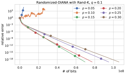
Refer to caption
Refer to caption
Refer to caption
Refer to caption
Figure 3: Performance of Rand-DIANA with the Rand-K sparsification operator for different values of p𝑝p.

Consider an 2subscript2\ell_{2}-regularized logistic regression optimization problem with the w2a dataset from the LibSVM repository (Chang and Lin, 2011).

fi(x)1ml=1mlog(1+exp(Ai,lxbi,l))+λ2x2,subscript𝑓𝑖𝑥1𝑚superscriptsubscript𝑙1𝑚1superscriptsubscriptA𝑖𝑙top𝑥subscript𝑏𝑖𝑙𝜆2superscriptnorm𝑥2f_{i}(x)\coloneqq\frac{1}{m}\sum_{l=1}^{m}\log\left(1+\exp\left(-\mathrm{A}_{i,l}^{\top}x\cdot b_{i,l}\right)\right)+\frac{\lambda}{2}\|x\|^{2},

where λ𝜆\lambda is set to guarantee that the condition number of the loss function f𝑓f is equal to 100. Ai,ld,bi,l{1,1}formulae-sequencesubscriptA𝑖𝑙superscript𝑑subscript𝑏𝑖𝑙11\mathrm{A}_{i,l}\in\mathbb{R}^{d},b_{i,l}\in\{-1,1\} are the feature and label of l𝑙l-th data point on the i𝑖i-th worker. The “optimum” xsuperscript𝑥x^{\star} is obtained by running AGD (Accelerated Gradient Descent) for the whole dataset using one CPU core until f(x)21032superscriptnorm𝑓𝑥2superscript1032\|\nabla f(x)\|^{2}\leq 10^{-32}.

Refer to caption
Refer to caption
Figure 4: Comparison of DIANA and Randomized-DIANA. Left plot: methods equipped with Rand-K for different q𝑞q values. Right plot: selected results of the grid search for Natural Dithering parameter s𝑠s over {2,,20}220\{2,\dots,20\}.

Conclusions are basically the same as the ones for Ridge Regression problem presented in Section 4.1, although DIANA performs slightly better with the Rand-K compressor for q=0.9𝑞0.9q=0.9.