Solving linear systems of the form $(A+\gamma UU^{T})\,{\bf x}={\bf b}$
by preconditioned iterative methods

Abstract.

We consider the iterative solution of large linear systems of equations in which the coefficient matrix is the sum of two terms, a sparse matrix $A$ and a possibly dense, rank deficient matrix of the form $\gamma UU^{T}$, where $\gamma>0$ is a parameter which in some applications may be taken to be 1. The matrix $A$ itself can be singular, but we assume that the symmetric part of $A$ is positive semidefinite and that $A+\gamma UU^{T}$ is nonsingular. Linear systems of this form arise frequently in fields like optimization, fluid mechanics, computational statistics, and others. We investigate preconditioning strategies based on an alternating splitting approach combined with the use of the Sherman-Morrison-Woodbury matrix identity. The potential of the proposed approach is demonstrated by means of numerical experiments on linear systems from different application areas.

Keywords:augmented systems, saddle point problems, augmented Lagrangian method, Schur complement, iterative methods, Krylov subspace methods, preconditioning techniques

2010 AMS Subject Classification: 65F10.

1. Introduction

A problem that frequently arises in large-scale scientific computing is the solution of linear systems of the form

(1) $$(A+\gamma UU^{T})\,x=b\,,$$

where $A\in\mathbb{R}^{n\times n}$, $U\in\mathbb{R}^{n\times k}$, $\gamma>0$ and ${\bf b}\in\mathbb{R}^{n}$ are given. We make the following assumptions:

• The matrix $A$ is positive semidefinite, in the sense that the symmetric matrix $A+A^{T}$ is positive semidefinite (sometimes, the term semipositive real is used).

• The matrix $A+\gamma UU^{T}$ is nonsingular; that is, ${\rm Ker}(A)\cap{\rm Ker}(U^{T})=\{{\bf 0}\}$.

• The number of columns $k$ of $U$ satisfies $k<n$ (and often $k\ll n$).

• Forming $A+\gamma UU^{T}$ explicitly would lead to loss of sparsity/structure and should be avoided.

Linear systems of the form (1) with such features arise for instance in the solution of the augmented Lagrangian formulation of saddle point problems, in the solution of reduced KKT systems from interior point methods in constrained optimization, and in the solution of sparse-dense least-squares problems.

In principle, approaches based on the Sherman-Morrison-Woodbury (SMW) matrix identity (see [23]) could be used to solve (1), assuming that systems with coefficient matrix $A$ can be solved efficiently. In this paper we focus mostly on situations where such an approach is not viable; for example, $A$ can be singular, and/or the problem size is too large for linear systems with $A$ to be solved accurately. Nevertheless, the SMW identity will play an important role in this paper, albeit not applied directly to (1).

Our focus is on the construction of preconditioners tailored to problem (1), to be used in conjunction with Krylov subspace methods. Since Krylov methods only need the coefficient matrix in the form of matrix-vector products, it is not necessary to explicitly add the two terms comprising the matrix $A+\gamma UU^{T}$, as long as matrix-vector products involving the matrices $A$, $U$ and $U^{T}$ can be performed efficiently. Our main goal, then, is to develop preconditioners that can be set up without explicitly forming $A+\gamma UU^{T}$, but working only with $A$, $U$ and $U^{T}$. The preconditioners must be inexpensive to construct and to apply, and effective at producing fast convergence of the preconditioned Krylov method. Robustness with respect to $\gamma$ is also highly desirable.

The remainder of the paper is organized as follows. In section 2 we discuss motivating examples for the proposed solution techniques, which will be described in section 3. In section 4 we briefly review some related work, while in section 5 we present some estimates on the eigenvalues of preconditioned matrices. Numerical experiments aimed at illustrating the performance of the proposed solvers are presented in section 6; conclusions and suggestions for future work are given in section 7.

2. Motivation

Large linear systems of the form (1) arise frequently in scientific computing. Examples include:

• Augmented Lagrangian methods for PDE-related saddle point problems [5, 11, 13, 20, 21, 22];

• Solution of KKT systems in constrained optimization [30];

• Solution of sparse-dense least squares problems [35, 36, 37];

• Solution of PDEs modeling almost incompressible materials [15, Ch. 8];

• Numerical solution of PDEs with nonlocal BC’s [24].

Another situation where systems of the form (1) may arise is when solving singular linear systems with a known kernel.

Next, we describe in some detail linear systems of the form (1) from the first three of these applications.

2.1. Linear systems from the augmented Lagrangian formulation

Consider the saddle point problem

$${\mathcal{A}}\,{\bf x}=\begin{bmatrix}A&B^{T}\\ B&0\end{bmatrix}\begin{bmatrix}u\\ p\end{bmatrix}=\begin{bmatrix}f\\ g\end{bmatrix}={\bf f}.$$

Such systems arise frequently from the finite element discretization of systems of PDEs, such as for example the Stokes equations, the Oseen problem (obtained from the steady Navier-Stokes equations via Picard linearization), or from first-order system formulations of second-order elliptic PDEs; see, e.g., [15, 19]. A powerful approach to solve such systems is the one based on the augmented Lagrangian formulation [21]. This method is also widely used for solving constrained optimization problems [30]. The idea is to replace the original saddle point problem with an equivalent one of the form:

$${\mathcal{A}}_{\gamma}\,{\bf x}=\begin{bmatrix}A+\gamma B^{T}W^{-1}B&B^{T}\\ B&0\end{bmatrix}\begin{bmatrix}u\\ p\end{bmatrix}=\begin{bmatrix}\hat{f}\\ g\end{bmatrix}=\hat{\bf f}\,,$$

where $\gamma>0$ and $\hat{f}:=f+\gamma B^{T}W^{-1}g$. Here $W$ is usually diagonal and positive definite. In the setting of finite element models of fluid flow, $W$ is often the diagonal of the (pressure) mass matrix. This new, augmented system is then solved by a Krylov subspace method with preconditioner

(2) $${\mathcal{P}}_{\gamma}=\begin{bmatrix}A+\gamma B^{T}W^{-1}B&B^{T}\\ 0&-\gamma^{-1}W\,.\end{bmatrix}$$

The convergence of the preconditioned iteration is very fast independent of parameters like the mesh size and (for the Oseen problem) the viscosity, especially for large $\gamma$ (see [11, 20]); to be practical, however, the preconditioner must be applied inexactly. Evidently, the only difficulty in applying the preconditioner is the solution of linear systems associated with the (1,1) block, i.e., a linear system with coefficient matrix $A+\gamma B^{T}W^{-1}B$ must be solved at each application of the preconditioner. This linear system is of the form (1) with $U=B^{T}W^{-1/2}$. Here $A$ is sparse, often block diagonal, and positive definite (or $A+A^{T}$ is). Forming $A+\gamma B^{T}W^{-1}B$ explicitly leads to loss of structure, and depending on the discretization used the resulting matrix can be considerably less sparse than $A$. The condition number increases with $\gamma$, and solving this system is the main challenge associated with the augmented Lagrangian approach; hence, the need to develop efficient iterative methods for it. In [11] and [20], specialized geometric multigrid methods have been developed for this task. While these methods have proven efficient, they suffer from the limitations of geometric multigrid methods, primarily the fact that they are tied to very specific types of meshes and discretizations. Here we consider algebraic approaches that can be applied to very general situations. We note that our preconditioned iteration being non-stationary, it will require the (inexact) augmented Lagrangian preconditioner ${\mathcal{P}}_{\gamma}$ to be used as a (right) preconditioner for Flexible GMRES [33]. For symmetric problems, the Flexible Conjugate Gradient method may also be viable under certain conditions [31].

The solution of linear systems of the form (1) is also required by the Relaxed Dimensional Factorization (RDF) preconditioner [10, 7], which has been developed in particular for the Oseen problem. Here $A$ is the discretization of a (scalar) convection-diffusion operator and $U^{T}$ represents the discretization of the partial derivative with respect to one of the space variables. For 3D problems, three such linear systems must be solved at each application of the preconditioner.

2.2. Schur complement systems arising from Interior Point methods

The solution of (smooth) constrained minimization problems by Interior Point (IP) methods (see [30]) leads to sequences of linear systems of the form

$${\mathcal{A}}\,{\bf x}=\begin{bmatrix}H&-C^{T}&0\\ C&0&-I_{k}\\ 0&Z&\Lambda\end{bmatrix}\begin{bmatrix}\delta x\\ \delta\lambda\\ \delta z\end{bmatrix}=\begin{bmatrix}-r_{1}\\ -r_{2}\\ -r_{3}\end{bmatrix}={\bf f}.$$

Here $H=H^{T}$ is the $n\times n$ Hessian of the objective function at the current point $\bar{x}$, $C$ is the $k\times n$ Jacobian of the constraints at the same point, and $Z$ and $\Lambda$ are diagonal, positive definite $k\times k$ matrices associated with the current values of the Lagrange multipliers $\bar{\lambda}$ and slack variables $\bar{z}$, respectively. The right-hand sides contains the nonlinear residuals. The variable $\delta z$ can easily be obtained using the last equation:

$$\delta z=-\Lambda^{-1}(r_{3}+Z\delta\lambda)$$

and substituted into the second (block) equation. This yields the reduced system

$$\begin{bmatrix}H&-C^{T}\\ C&\Lambda^{-1}Z\end{bmatrix}\begin{bmatrix}\delta x\\ \delta\lambda\end{bmatrix}=\begin{bmatrix}-r_{1}\\ -r_{2}-\Lambda^{-1}r_{3}\end{bmatrix}.$$

Eliminating $\delta\lambda$ leads to the fully reduced (Schur complement) system

(3) $$(H+C^{T}Z^{-1}\Lambda C)\delta x=-r_{1}-C^{T}Z^{-1}(r_{3}+\Lambda r_{2})=:b.$$

After solving for $\delta x$, the other unknowns $\delta\lambda$ and $\delta z$ are readily obtained. This system is of the form (1) with $A=H$, $U=C^{T}(Z^{-1}\Lambda)^{1/2}$ and $\gamma=1$. The coefficient matrix is nonsingular if and only if $\text{Ker}(H)\cap\text{Ker}(C)=\{0\}$. The Hessian is usually positive (semi)definite, sparse and possibly structured. The coefficient matrix is nonsingular if and only if $\text{Ker}(H)\cap\text{Ker}(C)=\{0\}$. Especially for very large problems, forming $H+C^{T}Z^{-1}\Lambda C$ explicitly is generally undesirable. Instead, we propose to solve the fully reduced system with PCG or another Krylov method using a suitable (algebraic) preconditioner.

2.3. Sparse-dense least squares problems

Consider a large linear least squares (LS) problem of the form

$$\|Bx-c\|_{2}=\min,$$

where $B\in\mathbb{R}^{m\times n}$, and $c\in\mathbb{R}^{m}$. We assume that $B$ has full column rank and that it has the following structure:

$$B=\begin{bmatrix}B_{1}\\ B_{2}\end{bmatrix}\,,\quad B_{1}\in\mathbb{R}^{(m-k)\times n},\quad B_{2}\in\mathbb{R}^{k\times n},$$

where $B_{1}$ is sparse and $B_{2}$ is dense. Then the LS problem is equivalent to the $n\times n$ system of normal equations:

(4) $$B^{T}Bx=(B_{1}^{T}B_{1}+B_{2}^{T}B_{2})x=B^{T}c\,,$$

which is of the form (1) with $A=B_{1}^{T}B_{1}$, $U=B_{2}^{T}$, $\gamma=1$ and $b=B^{T}c$. Once again, we would like to solve this system by an iterative method, so the matrix $B^{T}B$ is never formed explicitly. The main challenge is again constructing an effective preconditioner.

Recently, sparse-dense LS problems and various methods for their solution have been investigated in [35, 36, 37].

3. The proposed method and its variants

In this section we first describe a stationary iterative method for solving (1), then we develop a more practical preconditioner based on this solver. Although not strictly necessary, we assume that the coefficient matrix $A_{\gamma}:=A+\gamma UU^{T}$ is nonsingular for all $\gamma>0$. As we have seen in the previous section, in many applications the matrix $A$ (or $A+A^{T}$) is usually at least positive semidefinite, and we will make this assumption. Then the nonsingularity of $A_{\gamma}$ is equivalent to the condition

$$\textnormal{Ker}\,(A)\cap\textnormal{Ker}\,(U^{T})=\{0\}\,,$$

hence if $A$ is symmetric positive semidefinite and the above condition holds, then $A_{\gamma}$ is symmetric positive definite (SPD) for all $\gamma>0$.

When $A$ is nonsingular, one could use the Sherman-Morrison-Woodbury (SMW) formula to solve (1), but this can be expensive for large problems. Recall that SMW states that

$$(A+\gamma UU^{T})^{-1}=A^{-1}-\gamma A^{-1}U(I_{k}+\gamma U^{T}A^{-1}U)^{-1}U^{T}A^{-1},$$

hence $k+1$ linear systems of size $n\times n$ with coefficient matrix $A$ and an additional $k\times k$ system must be solved “exactly”. Another possibility would be to build preconditioners based on the SMW formula, where the action of $A^{-1}$ is replaced by some inexpensive approximation, but our attempts in this direction were unsuccessful. Also, $A$ is frequently singular.

When $k$ is small (say, $k=10$ or less), then any good preconditioner for $A$ (or $A+\alpha I_{n}$, $\alpha>0$, if $A$ is singular) can be expected to give good results. In fact, using a Krylov method preconditioned with $A^{-1}$ yields convergence in at most $k+1$ steps, hence convergence should be fast if a good approximation of the action of $A^{-1}$ is available. However, if $k$ is in the hundreds (or larger), this approach is not appealing.

Hence, it is necessary to take into account both $A$ and $\gamma UU^{T}$ when building the preconditioner. We do this by forming a suitable product preconditioner, as follows.

Let $\alpha>0$ be a parameter and consider the two splittings

$$A+\gamma UU^{T}=(A+\alpha I_{n})-(\alpha I_{n}-\gamma UU^{T})$$

and

$$A+\gamma UU^{T}=(\alpha I_{n}+\gamma UU^{T})-(\alpha I_{n}-A).$$

Note that both $A+\alpha I_{n}$ and $\alpha I_{n}+\gamma UU^{T}$ are invertible under our assumptions. Let $x^{(0)}\in\mathbb{R}^{n}$ and consider the alternating iteration

(5) $$\begin{cases}\,(A+\alpha I_{n})\,x^{(k+1/2)}=(\alpha I_{n}-\gamma UU^{T})\,x^{(k)}+b\,,\\ \,(\alpha I_{n}+\gamma UU^{T})\,x^{(k+1)}=(\alpha I_{n}-A)\,x^{(k+1/2)}+b\,,\end{cases}$$

with $k=0,1,\ldots$ This alternating scheme is analogous to that of other well-known iterative methods like ADI [14], HSS [4], MHSS [4], RDF [10], etc. Similar to these methods, we have the following convergence result.

Theorem 3.1.

If $A+A^{T}$ is positive definite, the sequence $\{x^{(k)}\}$ defined by (5) converges, as $k\to\infty$, to the unique solution of equation (1), for any choice of $x^{(0)}$ and for all $\alpha>0$.

Proof.

First we observe that under our assumptions the linear system (1) has a unique solution. Eliminating the intermediate vector $x^{(k+1/2)}$, we can rewrite (5) as a one-step stationary iteration of the form

$$x^{(k+1)}=T_{\alpha}x^{(k)}+d\,,\qquad k=0,1,\ldots,$$

where $d$ is a suitable vector and the iteration matrix $T_{\alpha}$ is given by

$$T_{\alpha}=(\alpha I_{n}+\gamma UU^{T})^{-1}(\alpha I_{n}-A)(\alpha I_{n}+A)^{-1}(\alpha I_{n}-\gamma UU^{T}).$$

This matrix is similar to

$$\hat{T}_{\alpha}=(\alpha I_{n}-A)(\alpha I_{n}+A)^{-1}(\alpha I_{n}-\gamma UU^{T})(\alpha I_{n}+\gamma UU^{T})^{-1}\,,$$

hence the spectral radius of $T_{\alpha}$ satisfies

$$\rho(T_{\alpha})=\rho(\hat{T}_{\alpha})\leq\|\hat{T}_{\alpha}\|_{2}\leq\|(\alpha I_{n}-A)(\alpha I_{n}+A)^{-1}\|_{2}\|(\alpha I_{n}-\gamma UU^{T})(\alpha I_{n}+\gamma UU^{T})^{-1}\|_{2}\,.$$

The first norm on the right-hand side is strictly less than 1 for $\alpha>0$ since the symmetric part of $A$ is positive definite (this result is sometimes referred to as “Kellogg’s Lemma”, see [27, page 13]), while the second one is obviously equal to 1 for all $\alpha>0$, since $UU^{T}$ is symmetric positive semidefinite and singular. Therefore $\rho(T_{\alpha})<1$ and the iteration is convergent for all $\alpha>0$. ∎

Remark 3.2.

If $A+A^{T}$ is only positive semidefinite, then all we can say is that $\rho(T_{\alpha})\leq 1$ and that 1 is not an eigenvalue of $T_{\alpha}$, for all $\alpha>0$. In this case we can still use the iterates $x^{(k)}$ to construct a convergent sequence that approximates the unique solution of (1); indeed, it is enough to replace $T_{\alpha}$ with $(1-\beta)\,I_{n}+\beta\,T_{\alpha}$, with $\beta\in(0,1)$, to obtain a convergent sequence; see [8, p. 27].

In practice, the stationary iteration (5) may not be very efficient. It requires exactly solving two linear systems with matrices $A+\alpha I_{n}$ and $\alpha I_{n}+\gamma UU^{T}$ at each step; even if these two systems are generally easier to solve than the original system (1), convergence can be slow and the overall method expensive. To turn this into a practical method, we will use it as a preconditioner for a Krylov-type method rather than as a stationary iterative scheme. This will also allow inexact solves.

To derive the preconditioner we eliminate $x^{(k+1/2)}$ from (5) and write the iterative scheme as the fixed-point iteration

$$x^{(k+1)}=T_{\alpha}x^{(k)}+c=(I_{n}-P_{\alpha}^{-1}A_{\gamma})x^{(k)}+P_{\alpha}^{-1}b\,.$$

An easy calculation (see also [12]) reveals that the preconditioner $P_{\alpha}$ is given, in factored form, by

(6) $$P_{\alpha}=\frac{1}{2\alpha}(A+\alpha I_{n})(\alpha I_{n}+\gamma UU^{T}).$$

The scalar factor $\frac{1}{2\alpha}$ in (6) is immaterial for preconditioning, and can be ignored in practice. Applying this preconditioner within a Krylov method requires, at each step, the solution of two linear systems with coefficient matrices $A+\alpha I_{n}$ and $\alpha I_{n}+\gamma UU^{T}$. Consider first solves involving $A+\alpha I_{n}$. If $A$ is sparse and/or structured (e.g., block diagonal, banded, Toeplitz, etc.), then so is $A+\alpha I_{n}$. If expensive, exact solves with $A+\alpha I_{n}$ can be replaced, if necessary, with inexact solves using either a good preconditioner for $A+\alpha I_{n}$, such as an incomplete factorization, or a fixed number (one may be enough) of cycles of some multigrid method if $A$ originates from a second-order elliptic PDE. We note here a typical trade-off: larger values of $\alpha$ make solves with $A+\alpha I_{n}$ easier (since the matrix becomes better conditioned and more diagonally dominant), but may degrade the performance of the preconditioner $P_{\alpha}$. In practice, we found that high accuracy is not required in the solution of linear systems associated with $A+\alpha I_{n}$.

On the other hand, numerical experiments suggest that the solution of linear systems involving $\alpha I_{n}+\gamma UU^{T}$ is more critical. Note that this matrix is SPD for all $\alpha>0$, but ill-conditioned for small $\alpha$ (or very large $\gamma$). The Sherman-Morrison-Woodbury formula yields

(7) $$(\alpha I_{n}+\gamma UU^{T})^{-1}=\alpha^{-1}I_{n}-\alpha^{-1}\gamma U(\alpha I_{k}+\gamma U^{T}U)^{-1}U^{T}.$$

The main cost is the solution at each step of a $k\times k$ linear system with matrix $\alpha I_{k}+\gamma U^{T}U$, which can be performed by Cholesky factorization (computed once and for all at the outset) or possibly by a suitable inner PCG iteration or maybe an (algebraic) MG method. Formula (7) shows why this $k\times k$ linear system must be solved accurately: any error affecting $(\alpha I_{k}+\gamma U^{T}U)^{-1}$, and therefore $U(\alpha I_{k}+\gamma U^{T}U)^{-1}U^{T}$, will be be amplified by the factor $\gamma/\alpha$, which will be quite large for small $\alpha$ and large or even moderate values of $\gamma$. Note that for linear systems arising from the augmented Lagrangian method applied to incompressible flow problems, the matrix $\alpha I_{k}+\gamma U^{T}U$ is a (shifted and scaled) discrete pressure Laplacian. Also, this matrix remains constant in the course of the numerical solution of the Navier–Stokes equations using Picard or Newton iteration, whereas the matrix $A$ changes. Hence, the cost of a Cholesky factorization of $\alpha I_{k}+\gamma U^{T}U$ can be amortized over many nonlinear (or time) steps. Similar observations apply if one uses an algebraic multigrid (AMG) solver instead of a direct factorization, in the sense that the preconditioner set-up needs to be done only once.

3.1. Some variants

Building on the main idea, different variants of the preconditioner can be envisioned. If $A$ happens to be nonsingular and linear systems with $A$ are not too difficult to solve (inexactly or perhaps even exactly), then it may not be necessary to shift $A$, leading to a preconditioner of the form

$$\hat{P}_{\alpha}=A(\alpha I_{n}+\gamma UU^{T}).$$

Note that Theorem 3.1, however, is no longer applicable in general.

When $A$ is symmetric positive semidefinite and the usual assumption $\textnormal{Ker}\,(A)\cap\textnormal{Ker}\,(U^{T})=\{0\}$ holds (so that $A_{\gamma}$ is SPD for $\gamma>0$), one would like to solve system (1) using the preconditioned conjugate gradient (PCG) method. Unless $A$ and $UU^{T}$ commute, however, the preconditioner (6) is nonsymmetric, and the preconditioned matrix $P_{\alpha}^{-1}A_{\gamma}$ is generally not symmetrizable. In this case we can consider a symmetrized version of the preconditioner, for example

(8) $$P_{\alpha}^{S}=\frac{1}{2\alpha}L\,(\alpha I_{n}+\gamma UU^{T})\,L^{T}\,,$$

where $L$ is the Cholesky (or incomplete Cholesky) factor of $A+\alpha I_{n}$ (or of $A$ itself if $A$ is SPD and not very ill-conditioned). Again, Theorem 3.1 no longer holds, in general.

In some cases (but not always) the performance of the method improves if $A_{\gamma}$ is diagonally scaled so that it has unit diagonal prior to forming the preconditioner. Note that the matrix

$$D_{\gamma}:=\text{diag}\,(A+\gamma UU^{T})$$

can be easily computed:

$$(D_{\gamma})_{ii}=a_{ii}+\gamma\|u_{i}^{T}\|_{2}^{2}\,,$$

where $u_{i}^{T}$ is the $i$th row of $U$. It is easy to see that applying the preconditioner to the diagonally scaled matrix $D_{\gamma}^{-1/2}A_{\gamma}D_{\gamma}^{-1/2}$ is mathematically equivalent to using the modified preconditioner

$$(A+\alpha D_{\gamma})D_{\gamma}^{-1}(\alpha D_{\gamma}+\gamma UU^{T})$$

on the original matrix. We emphasize that whether this diagonal scaling is beneficial or not appears to be strongly problem-dependent. Numerical experiments indicate that such scaling can lead to a degradation of performance in some cases. Clearly, different SPD matrices (other than the diagonal of $A_{\gamma}$) could be used for $D_{\gamma}$.

One can also conceive two-parameter variants, $P_{\alpha,\beta}=(A+\alpha I_{n})(\beta I_{n}+\gamma UU^{T})$, but we shall not pursue such generalizations here.

Finally, we observe that the extension to the complex case (under the obvious assumptions) is straightforward.

4. Related work

There seems to have been relatively little work on the development of specific solvers for linear systems of the form (1). The few papers we are aware of either advocate for the use of the SMW formula directly applied to (1), or treat specialized methods for very specific situations.

In the recent papers [25, 26], the author addresses the solution of linear systems closely related to (1) by means of an auxiliary space preconditioning approach. This approach is specific to finite element discretizations of PDE problems involving the De Rham complex and the Hodge Laplacian, such as those arising from the solution of the curl-curl formulation of Maxwell’s equations.

Potentially relevant to our approach is the work on robust multigrid preconditioners for finite element discretizations of the operator $\mathcal{L}=I-\gamma\,\text{grad}\,\text{div}$, defined on the space $H(\text{div})$. Indeed, for the type of incompressible flow problems described in section 2.1 the matrix $\alpha I_{n}+\gamma UU^{T}$ may be regarded as a discretized version of this operator, which plays an important role in several applications; see, e.g., [2, 3, 28]. In cases where direct use of the SMW formula for solving linear systems with matrix $\alpha I_{n}+\gamma UU^{T}$ is not viable, for example in very large 3D situations where Cholesky factorization of a $k\times k$ matrix may be too expensive, such multigrid methods could be an attractive alternative in view of their robustness and fast convergence.

Finally, we mention the work in [16], although it concerns a somewhat different type of problem, namely, linear systems with coefficient matrix of the form $A+UCU^{T}$ with $A=A^{T}$ and $C=-C^{T}$. Here $U\in\mathbb{R}^{n\times k}$ and $C\in\mathbb{R}^{k\times k}$. We point out that for this type of problem, our approach reduces to the well-known HSS method (or preconditioner), see [4].

5. Eigenvalue bounds

As is also the case for other solvers and preconditioners like ADI or HSS, the choice of $\alpha$ is important for the success of the method. It is not easy to determine an “optimal” or even good value of $\alpha$ a priori. Usually it is necessary to resort to heuristics, one of which will be discussed in the next section. Here we attempt to shed some light on the effect of $\alpha$ on the spectrum of the preconditioned matrix $P_{\alpha}^{-1}A_{\gamma}$. Note that by virtue of Theorem 3.1 and Remark 3.2, we know that the spectrum of $\sigma(P_{\alpha}^{-1}A_{\gamma})$ lies in the disk of center $(1,0)$ and radius 1 in the complex plane, for all $\alpha>0$. In particular, all the eigenvalues have imaginary part bounded by 1 in magnitude.

First we consider the case where $A$ is SPD. Let $0<\lambda_{1}\leq\cdots\leq\lambda_{n}$ be the eigenvalues of $A$. As shown in the proof of Theorem 3.1, the spectral radius of the iteration matrix $T_{\alpha}=I_{n}-P_{\alpha}^{-1}A_{\gamma}$ of the stationary iteration (5) satisfies

$$\rho(T_{\alpha})\leq\|(\alpha I_{n}-A)(\alpha I_{n}+A)^{-1}\|_{2}=\max_{1\leq i\leq n}\frac{|\alpha-\lambda_{i}|}{|\alpha+\lambda_{i}|}\,,$$

for all $\alpha>0$. The upper bound on $\rho(T_{\alpha})$ is minimized, as is well known, taking $\alpha=\sqrt{\lambda_{1}\lambda_{n}}$. A similar observation, incidentally, has been made for the HSS method in [4], with the eigenvalues of $H=\frac{1}{2}(A+A^{T})$ playing the role of the $\lambda_{i}$’s. This choice of $\alpha$ is completely independent of $\gamma$ and $U$, and thus it is not likely to be always a good choice, especially when the method is used as a preconditioner rather than as a stationary solver.

In order to state the next result, we note that there is no loss of generality if we assume that $\|A\|_{2}=1$ and $\|U\|_{2}=1$, since we can always divide both sides of (1) by $\|A\|_{2}$, replace $\gamma$ with $\tilde{\gamma}:=\gamma\|U\|_{2}^{2}/\|A\|_{2}$ and $U$ with $\tilde{U}:=U/\|U\|_{2}$.

Theorem 5.1.

Let $A$ be such that $A+A^{T}$ is positive definite. Assume that $\|A\|_{2}=\|U\|_{2}=1$. Let $P_{\alpha}$ be given by (6). If $(\lambda,x)$ is a real eigenpair of the preconditioned matrix $P_{\alpha}^{-1}A_{\gamma}$, with $\|x\|_{2}=1$, then $\lambda\in[\mu,2)$ where

(9) $$\mu=\frac{\alpha\,\lambda_{\min}(A+A^{T})}{(1+\alpha)(\alpha+\gamma)}.$$

If $(\eta,x)$ is an eigenpair of $A$ with $x\in\textnormal{Ker}\,(U^{T})$, then $x$ is eigenvector of $P_{\alpha}^{-1}A_{\gamma}$ associated to the eigenvalue

(10) $$\lambda=\frac{2\,\eta}{\eta+\alpha}$$

(independent of $\gamma$).

Proof.

The eigenpairs $(\lambda,x)$ of $P_{\alpha}^{-1}A_{\gamma}$ (or, equivalently, of $A_{\gamma}P_{\alpha}^{-1}$) satisfy the generalized eigenvalue problem

(11) $$(A+\gamma UU^{T})\,x=\frac{\lambda}{2\alpha}\,(\alpha A+\gamma AUU^{T}+\alpha^{2}I_{n}+\alpha\,\gamma\,UU^{T})\,x\,.$$

Premultiplying by $x^{*}$ and using $x^{*}x=1$, we obtain

(12) $$\lambda=\frac{2\alpha\,(x^{*}Ax+\gamma\|U^{T}x\|_{2}^{2})}{\alpha\,x^{*}Ax+\gamma\,x^{*}AUU^{T}x+\alpha^{2}+\alpha\,\gamma\,\|U^{T}x\|_{2}^{2}}\,.$$

If $\lambda$ is real then $x$ can be taken real and $x^{*}$ becomes $x^{T}$. Clearly $0<\lambda<2$ as an immediate consequence of Theorem 3.1, which states that $|\lambda-1|<1$. To prove the lower bound on $\lambda$, note that a lower bound on the numerator in (12) is given by $\alpha\,\lambda_{\min}(A+A^{T})$, while an upper bound for the denominator is given by $\alpha+\gamma+\alpha^{2}+\alpha\gamma=(1+\alpha)(\alpha+\gamma)$, yielding the value (9) for the lower bound on $\lambda$.

If $U^{T}x=0$ we immediately obtain (10) from (12). Note that all such $\lambda$’s (if there are any) are necessarily real if $A=A^{T}$. ∎

Remark 5.2.

If we assume $A$ to be symmetric positive definite, then using (12) one can easily establish the following lower bound on the real part of the eigenvalues of $P_{\alpha}^{-1}A_{\gamma}$, whether real or not:

(13) $$Re(\lambda)\geq\frac{2\,\alpha(\alpha+1)(\alpha+\gamma)\,\lambda_{\min}(A)}{(\alpha+1)^{2}(\alpha+\gamma)^{2}+\gamma^{2}}\,.$$

We computed the eigenvalues in several cases with an SPD matrix $A$ (see next section) and we found that usually the lower bound given by (9) yields a much better estimate of the smallest real part of $\lambda\in\sigma(P_{\alpha}^{-1}A_{\gamma})$ than (13), suggesting that the eigenvalue of smallest real part is actually real in many cases. Our experiments confirm that when $A$ is SPD, the smallest eigenvalue of $P_{\alpha}^{-1}A_{\gamma}$ is often real, but this is not true in general. Note that all the bounds still hold if $A$ is singular, but give no useful information in this case.

Remark 5.3.

If $A$ is singular and if $(\lambda,x)$ is an eigenpair of $P_{\alpha}^{-1}A_{\gamma}$ with $x\in\textnormal{Ker}(A^{T})$, then $U^{T}x\neq 0$ and

$$\lambda=\frac{2}{1+\frac{\alpha}{\gamma\|U^{T}x\|_{2}^{2}}}$$

(independent of $A$). Indeed, we have $x^{*}Ax=0$ and $x^{*}AUU^{T}x=0$. Thus, (12) reduces to

$$\lambda=\frac{2\,\alpha\,\gamma\|U^{T}x\|_{2}^{2}}{\alpha^{2}+\alpha\,\gamma\,\|U^{T}x\|_{2}^{2}}\,$$

Clearly $U^{T}x\neq 0$ since we are assuming that $A_{\gamma}$ is nonsingular. Dividing the numerator and denominator by $\alpha\,\gamma\,\|U^{T}x\|_{2}^{2}$ we obtain the result. Note that such a $\lambda$, if it exists, is real.

Remark 5.4.

Theorem 5.1 is of limited use for guiding in the choice of $\alpha$. It is easy to see that the lower bound (9) is maximized (when $A$ is nonsingular) by taking $\alpha=\sqrt{\gamma}$. While such a choice of $\alpha$ may prevent the smallest eigenvalue of the preconditioned matrix from getting too close to 0, in most cases such value of $\alpha$ is suboptimal. We also note that the lower bound approaches zero as $\alpha\to 0$ and $\gamma\to\infty$, yet small values of $\alpha$ often yield faster convergence, even for large values of $\gamma$, suggesting that a better clustering of the preconditioned spectrum is achieved for smaller values of $\alpha$. One should also keep in mind that the result assumes that the preconditioner is applied exactly, which is often not the case in practice, and that eigenvalues alone may not be descriptive of the convergence of Krylov subspace methods like GMRES. Nevertheless, setting $\alpha=\sqrt{\gamma}$ could be a reasonable choice in the absence of other information, provided of course that the problem is scaled so that $\|A\|_{2}=\|U\|_{2}=1$.

We conclude this section with a result concerning the symmetrized preconditioner (8).

Theorem 5.5.

Let $A$ be SPD, $A_{\gamma}=A+\gamma UU^{T}$, with $\|A\|_{2}=1$ and $\|U\|_{2}=1$, and let $P_{\alpha}^{S}=\frac{1}{2\alpha}L\,(\alpha I_{n}+\gamma UU^{T})\,L^{T}$ where $L$ is the Cholesky factor of $A+\alpha I_{n}$. Then the eigenvalues $\lambda$ of the preconditioned matrix $(P_{\alpha}^{S})^{-1}A_{\gamma}$ are all real and lie in the interval

(14) $$\frac{2\,\alpha\,\lambda_{\min}(A)}{(1+\alpha)(\alpha+\gamma)}<\lambda<\frac{2+2\,\gamma}{\lambda_{\min}(A)+\alpha}\,.$$

Proof.

That the eigenvalues of the preconditioned matrix are real (and positive) is an immediate consequence of the fact that both the preconditioner $P_{\alpha}^{S}$ in (8) and the coefficient matrix $A_{\gamma}=A+\gamma UU^{T}$ are SPD. If $(\lambda,x)$ is an eigenpair of $(P_{\alpha}^{S})^{-1}A_{\gamma}$ then

$$\lambda=\frac{2\,\alpha\,\,x^{T}(A+\gamma UU^{T})\,x}{x^{T}L(\alpha I_{n}+\gamma UU^{T})L^{T}x}=\frac{2\,\alpha\,x^{T}Ax+2\,\alpha\,\gamma\,\|U^{T}x\|_{2}^{2}}{\alpha\,x^{T}Ax+\alpha^{2}\,+\gamma\,\|U^{T}L^{T}x\|_{2}^{2}}\,.$$

The lower bound in (14) is obtained my minimizing the numerator and maximizing the denominator in the last expression, keeping in mind that $\|x\|_{2}=1$ and that $\|U^{T}L^{T}\|_{2}^{2}\leq\|L^{T}\|_{2}^{2}=\|A+\alpha I_{n}\|_{2}=1+\alpha$. Similarly, the upper bound is obtained by maximizing the numerator and minimizing the denominator in the last expression. ∎

We remark that the lower bound in (14) is identical to the one in (9) since now $A=A^{T}$. The bound suggests the possibility of a high condition number for $(P_{\alpha}^{S})^{-1}A_{\gamma}$ if $A$ is ill-conditioned (small $\lambda_{\min}(A)$), if $\alpha$ is very small, or if $\gamma$ is very large. On the other hand, it is well known that estimates of the rate of convergence of the PCG method based on the condition number can be very pessimistic, particularly in the presence of eigenvalue clustering. Also, we found that the upper bound in (14) tends to be rather loose.

6. Numerical experiments

In this section we describe the results of numerical experiments with several matrices from the three application areas discussed in section 2. First we present the results of some computations aimed at assessing the quality of the eigenvalue bounds on $Re(\lambda)$ given in Theorem 5.1, then we provide an evaluation of the performance of the proposed preconditioners in terms of iteration counts and timings on a selection of test problems. All the computations were performed using MATLAB.R2020b on a laptop with a 4 Intel core i7-8565U CPU @ 1.80GHz - 1.99 GHz and 16.0GB RAM.

6.1. Eigenvalue bounds

Here we consider matrices arising from the following three problems:

1. A stationary Stokes problem discretized with Q2-Q1 mixed finite elements on a uniform $64\times 64$ mesh;

2. A stationary Oseen problem with viscosity $\nu=0.01$ discretized with Q2-Q1 mixed finite elements on a stretched $64\times 64$ mesh;

3. A Schur complement arising from a KKT system in constrained optimization;

The first two matrices are generated using IFISS [18] and they are of the form $A_{\gamma}=A+\gamma B^{T}W^{-1}B$ where $A$ is the stiffness velocity matrix, $B^{T}$ the discrete gradient, and $W$ is the diagonal of the pressure mass matrix. Here $U^{T}=W^{-1/2}B$, $n=8450$ and $k=1089$. For the Stokes problem $A$ is SPD, for the Oseen problem $A\neq A^{T}$ but $A+A^{T}$ is SPD. In both cases the flow problem being modeled is the 2D leaky-lid driven cavity problem, see [19].

The third matrix is a Schur complement $H+C^{T}Z^{-1}\Lambda C$ obtained from reduction of a KKT system in constrained optimization [29]. Here $A=H$ is SPD, $U^{T}=(Z^{-1}\Lambda)^{1/2}C^{T}$, $\gamma=1$, $n=2500$ and $k=700$.

In all cases $A$ and $U$ have been normalized so that $\|A\|_{2}=\|U\|_{2}=1$. In Tables 1, 2 and 3 we report the minimum and maximum real part of the eigenvalues of $P_{\alpha}^{-1}A_{\gamma}$ together with the value of the estimate $\mu$ in (9). In Tables 1 and 2 we vary $\alpha$ and $\gamma$, in Table 3 we fix $\gamma=1$ and vary $\alpha$.

First we comment on the results for the linear systems arising from the incompressible Stokes and Oseen problems. In both cases the expression (9), which strictly speaking is a lower bound only for the real eigenvalues of the preconditioned matrix, is always a lower bound for the smallest $Re(\lambda)$ (here we only show a few values of $\alpha$ and $\gamma$, but the same was found in many more cases). We checked and found that for the preconditioned matrix $P_{\alpha}^{-1}A_{\gamma}$ associated with the Stokes problem, for which $A$ is SPD, the eigenvalue of smallest real part is in fact always real; hence, (9) is guaranteed to be a lower bound, as is confirmed by the results in Table 1. On the other hand, in the case of the matrix associated with the Oseen problem, for some combinations of $\alpha$ and $\gamma$ the eigenvalue with smallest real part was found to be non-real. Even in these cases, however, the estimate (9) yielded a lower bound on $Re(\lambda)$.

Generally speaking we see that the lower bound is reasonably tight, typically within an order of magnitude of the true value except in a few cases.

Table 1. Results for eigenvalues of preconditioned $A_{\gamma}$ matrix from Stokes problem with $64\times 64$ mesh and Q2-Q1 discretization. Here $A$ is SPD. In boldface the value $\alpha=\sqrt{\gamma}$.

$\gamma$	$\alpha$	$\max{(Re(\lambda))}$	$\min{(Re(\lambda))}$	lower bound (9)
0.1	0.1	1.818e+00	1.700e-02	5.709e-04
	0.3162	1.519e+00	5.409e-03	7.250e-04
	5.0	3.333e-01	3.430e-04	2.052e-04
1.0	0.5	1.333e+00	6.590e-03	2.791e-04
	1.0	1.000e+00	3.300e-03	3.140e-04
	5.0	4.683e-01	6.609e-04	1.744e-04
50.0	1.0	1.532e+00	3.323e-03	1.231e-05
	7.0711	1.658e+00	4.707e-04	1.928e-05
	10.0	1.606e+00	3.328e-04	1.903e-05

Table 2. Results for eigenvalues of preconditioned $A_{\gamma}$ matrix from Oseen problem with a stretched $64\times 64$ mesh, $\nu=0.01$, and Q2-Q1 discretization. Here $A\neq A^{T}$ but $A+A^{T}$ is SPD. In boldface the value $\alpha=\sqrt{\gamma}$.

$\gamma$	$\alpha$	$\max{(Re(\lambda))}$	$\min{(Re(\lambda))}$	lower bound (9)
0.1	0.1	1.818e+00	5.317e-03	1.581e-04
	0.3162	1.520e+00	1.684e-03	2.008e-04
	5.0	3.333e-01	1.066e-04	5.684e-05
1.0	0.5	1.333e+00	2.691e-03	7.730e-05
	1.0	1.000e+00	1.346e-03	8.697e-05
	5.0	4.423e-01	2.694e-04	4.831e-05
50.0	1.0	1.693e+00	9.185e-04	3.410e-06
	7.0711	1.668e+00	1.300e-04	5.340e-06
	10.0	1.613e+00	9.189e-05	5.271e-06

Table 3. Results for eigenvalues of preconditioned Schur complement matrix from KKT system (problem mosarqp1 from Maros and Mészáros collection). Here $A=H$ is SPD.

$\alpha$	$\max{(Re(\lambda))}$	$\min{(Re(\lambda))}$	lower bound (9)
0.001	1.998e+00	6.508e-03	7.343e-04
0.01	1.980e+00	6.321e-02	7.213e-03
0.1	1.818e+00	4.834e-01	6.081e-02
0.5	1.333e+00	8.484e-01	1.635e-01
1.0	1.000e+00	5.384e-01	1.839e-01
5.0	4.335e-01	1.372e-01	1.022e-01
10.0	2.457e-01	7.106e-02	6.081e-02
20.0	1.313e-01	3.617e-02	3.337e-02

Looking at the results reported in Table 3, we see that the bound is even more accurate for this (non PDE-related) problem. Furthermore, the eigenvalue distribution for this test case is especially favorable for the convergence of preconditioned iterations, suggesting fast convergence. For this particular problem we checked and found that the eigenvalue of smallest real part is always real, and actually all the eigenvalues of the preconditioned matrix are real.

We also note that in all cases the largest value of the lower bound corresponds to $\alpha={\sqrt{\gamma}}$, which is expected since the right-hand side of (9) attains its maximum for this value of $\alpha$.

6.2. Test results for problems from incompressible fluid mechanics

Here we present results obtained with the proposed approach on linear systems of the form

(15) $$(A+\gamma B^{T}W^{-1}B)\,x=b$$

associated with Stokes and Oseen problems. The matrices arise from Q2-Q1 discretizations of the driven cavity problem. We are interested in the performance of the solver with respect to the mesh size and the parameters $\alpha$ and $\gamma$. For both Stokes and Oseen, $A$ is block diagonal but $A_{\gamma}=A+\gamma B^{T}W^{-1}B$ is not.

In our experiments we use right-preconditioned restarted GMRES with restart $m=20$ [34]. The ideal preconditioner

$$P_{\alpha}=(A+\alpha I_{n})(\alpha I_{n}+\gamma B^{T}W^{-1}B)$$

is replaced by the inexact variant

(16) $$\tilde{P}_{\alpha}=M_{\alpha}(\alpha I_{n}+\gamma B^{T}W^{-1}B)\,,$$

where $M_{\alpha}=\tilde{L}\tilde{L}^{T}$ is the no-fill incomplete Cholesky (or, in the case of Oseen, incomplete LU) factorization of $A+\alpha I_{n}$; see, e.g., [6]. This approximation is inexpensive in terms of cost and memory and it greatly reduces the cost of the proposed preconditioner without adversely impacting its effectiveness. On the other hand, the factor $(\alpha I+\gamma B^{T}W^{-1}B)$ is inverted exactly via the SMW formula (7) with a sparse Cholesky factorization of the $k\times k$ matrix $\alpha I_{k}+\gamma W^{-1/2}BB^{T}W^{-1/2}$. The sparse Cholesky factorization makes use of the Approximate Minimum Degree (AMD) reordering strategy to reduce fill-in [1]. It is important to note that in the solution of the Navier–Stokes equations by Picard iteration, the matrices $B$ and $W$ of the Oseen problem remain constant throughout the solution process, hence the Cholesky factorization of $\alpha I_{k}+\gamma W^{-1/2}BB^{T}W^{-1/2}$ needs to be performed only once at the beginning of the process. The matrix $A$, on the other hand, changes at each Picard step (since the convective term changes). Recomputing the no-fill incomplete LU factorization of $A+\alpha I_{n}$, however, is inexpensive.

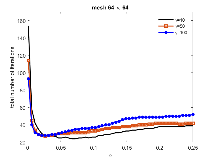
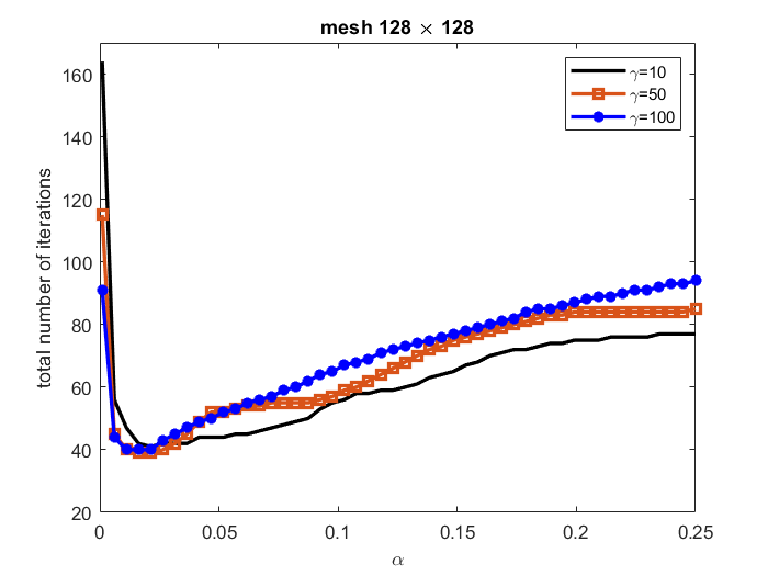
Figure 1. Number of preconditioned iterations versus $\alpha$ for the linear systems (15) arising from the 2D Stokes problem with Q2-Q1 finite element discretization on $64\times 64$ mesh (left) and on $128\times 128$ mesh (right) for different values of $\gamma$.

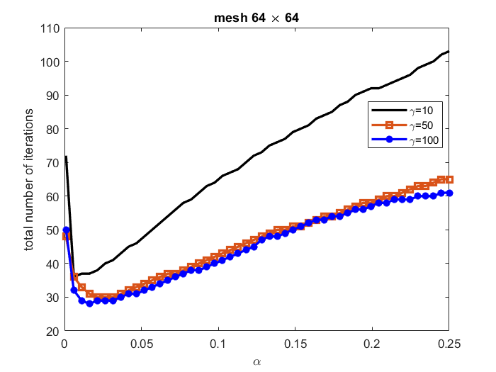
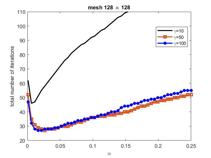
Figure 2. Number of preconditioned iterations versus $\alpha$ for the linear systems (15) arising from 2D Oseen problem with $\nu=0.01$, Q2-Q1 finite element discretization on stretched $64\times 64$ (left) and $128\times 128$ (right) meshes for different values of $\gamma$.

In Figures 1 and 2 we show results for linear systems of the form (15) arising from the Stokes and Oseen problems discretized on two meshes of size $64\times 64$ and $128\times 128$, for three different values of $\gamma$ ($=10,50,100$). Uniform meshes are used for the Stokes-related problem, stretched ones for the Oseen-related one. We apply a symmetric diagonal scaling to $A_{\gamma}$ prior to constructing the preconditioner. The plots show the number of right preconditioned GMRES(20) iterations (with the preconditioner (16)) as a function of the parameter $\alpha$. The stopping criterion used is $\|b-A_{\gamma}x_{k}\|_{2}<10^{-6}\|b\|_{2}$, with initial guess $x_{0}=0$. We mention that this stopping criterion is much more stringent than the one that would be used when performing inexact preconditioner solves in the context of the augmented Lagrangian preconditioner (2).

For the Stokes-related problem, the first observation is that the fastest convergence is obtained for small values of $\alpha$ and the number of iterations is fairly insensitive to the value of $\gamma$, at least for the range of $\alpha$ values showed. Also, if $\alpha$ is not too small, the curves are relatively flat and the number of iterations increases slowly with $\alpha$. As the mesh is refined the number of iterations increases, and the optimum $\alpha$ decreases slightly.

When passing from the Stokes to the Oseen-related problem (with viscosity $\nu=0.01$), the behavior of the solver is strikingly different. The convergence behavior is more sensitive to the value of $\gamma$; the fastest convergence is observed for larger values of $\gamma$, for which the matrix $A_{\gamma}$ is more ill-conditioned. This is probably due to the fact that the term $\gamma B^{T}W^{-1}B$ becomes dominant, and the factor $\alpha I_{n}+\gamma B^{T}W^{-1}B$ (with small $\alpha$) is a good approximation to $A_{\gamma}$. The location of the optimal value of $\alpha$ appears to be roughly the same as for the Stokes problem, but the curves are less flat and the number of iterations increases more rapidly as $\alpha$ moves away from the optimum. The most striking phenomenon, however, is that (contrary to the case of Stokes) the number of iterations appears to decrease as the mesh is refined. This finding is very welcome in view of the fact that the augmented Lagrangian approach is especially effective in the (challenging) case of the Oseen problem with small viscosity, as shown, e.g., in [11, 20]. We also note that the optimal $\alpha$ is independent of $\gamma$ when $\gamma$ is large enough.

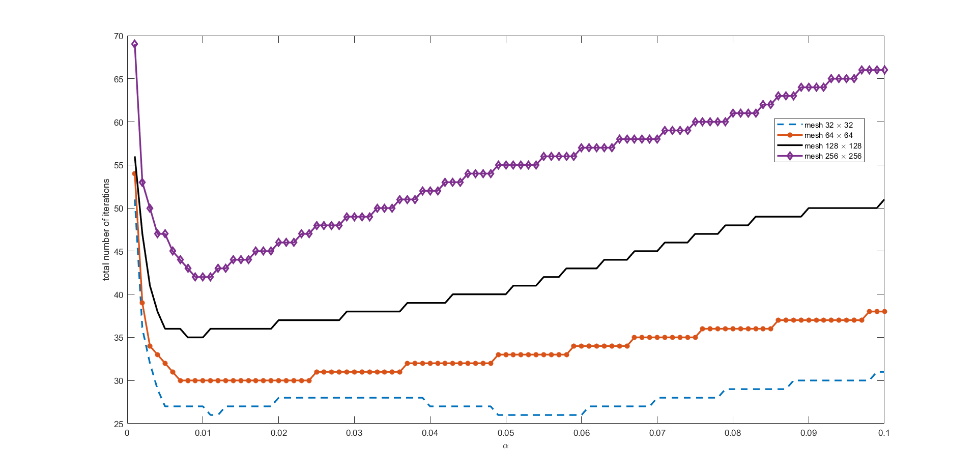
Figure 3. Number of iterations versus $\alpha$ for the linear systems (15) arising from the 2D Oseen problem with $\nu=0.1$, $\gamma=100$, Q2-Q1 finite element discretization and different mesh sizes. GMRES restart $m=20$, convergence residual tolerance = $10^{-6}$. Diagonal scaling is applied.

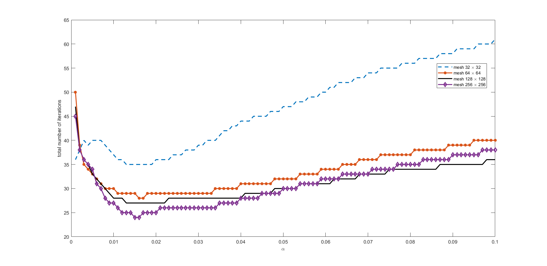
Figure 4. Number of iterations versus $\alpha$ for the linear systems (15) arising from the 2D Oseen problem with $\nu=0.01$, $\gamma=100$, Q2-Q1 finite element discretization and different mesh sizes. GMRES restart $m=20$, convergence residual tolerance = $10^{-6}$. Diagonal scaling is applied.

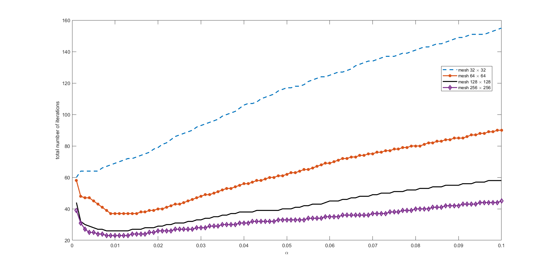
Figure 5. Number of iterations versus $\alpha$ for the linear systems (15) arising from the 2D Oseen problem with $\nu=0.002$, $\gamma=100$, Q2-Q1 finite element discretization and different mesh sizes. GMRES restart $m=20$, convergence residual tolerance = $10^{-6}$. Diagonal scaling is applied.

In Figures 3, 4 and 5 we show results for the Oseen-related problem for three different values of the viscosity $\nu$, discretized on four different (stretched) meshes. The value of $\gamma$ is fixed at 100. Several observations are in order. The number of iterations does not seem to be very sensitive to $\alpha$, as long as this is small, and the best $\alpha$ is about the same in all cases. The behavior of the solver improves as the mesh is refined and as the viscosity gets smaller, i.e., the harder the problem, the faster the convergence. This is especially welcome given that the augmented Lagrangian-based preconditioner is best employed on problems with small viscosity.

Table 4. Linear system from Oseen problem with $\gamma=100$. For each mesh we use $\alpha=0.011$ for $\nu=0.1$, $\alpha=0.0135$ for $\nu=0.01$, and $\alpha=0.009$ for $\nu=0.002$. Stretched Q2-Q1 finite element discretization. Diagonal scaling is used. $M_{\alpha}$ is ILU(0) of $A+\alpha I$, $\tilde{P}_{\alpha}=M_{\alpha}(\alpha I_{n}+\gamma UU^{T})$ with sparse Cholesky factorization of $k\times k$ matrix in SMW formula. M-Time and P-Time are the preconditioner construction times. Sol-Time is the time for the preconditioned iteration to achieve a relative residual norm below $10^{-6}$. All timings are in seconds.

				$M_{\alpha}$		$\tilde{P}_{\alpha}$
$\nu$	mesh	M-Time	P-Time	Sol-Time	Its	Sol-Time	Its
0.1	$32\times 32$	7.52e-04	1.39e-03	5.29e-02	173	6.75e-03	26
	$64\times 64$	1.22e-03	2.92e-03	3.83e-01	469	3.61e-02	30
	$128\times 128$	6.64e-03	1.54e-02	2.39e+00	603	2.41e-01	36
	$256\times 256$	2.48e-02	8.63e-02	2.03e+01	919	2.21e+00	42
0.01	$32\times 32$	7.26e-04	1.34e-03	1.56e-01	412	1.93e-02	35
	$64\times 64$	3.15e-03	1.48e-02	7.44e-01	466	5.61e-02	29
	$128\times 128$	1.29e-02	3.13e-02	3.05e+00	493	3.31e-01	27
	$256\times 256$	3.95e-02	1.38e-01	1.52e+01	486	1.53e+00	25
0.002	$32\times 32$	4.86e-04	9.36e-04	1.37e-01	754	1.42e-02	68
	$64\times 64$	1.35e-03	3.05e-03	4.89e-01	522	4.85e-02	37
	$128\times 128$	6.16e-03	1.51e-02	4.09e+00	1037	1.80e-01	26
	$256\times 256$	2.44e-02	8.26e-02	1.52e+01	767	1.06e+00	23

In Table 4 we report iteration counts and timings for the Oseen-related problems with the three values of $\nu=0.1,0.01,0.002$ for different mesh sizes and $\gamma=100$. For completeness we also include results obtained using the simple no-fill incomplete factorization $\tilde{L}\tilde{U}\approx A+\alpha I_{n}$ as a preconditioner for the system (15). Not surprisingly, this preconditioner yields very slow convergence, showing the importance of including the $\gamma$-dependent term in the preconditioner. Note that the cost of forming the preconditioner (16) is quite low, only slightly higher than the cost of $M_{\alpha}$, and that the iterative solution time dominates the overall cost. The results confirm the effectiveness of the proposed preconditioner, especially for small values of $\nu$ and finer meshes. We also note that the cost of the preconditioner construction is low compared to the overall solution costs, and it is dominated by the Cholesky factorization of the $k\times k$ matrix in the SMW formula. As already mentioned, when solving the Navier-Stokes equations this factorization needs to be performed only once since the matrix being factored does not change in the course of the Picard iteration.

6.3. Test results on Schur complements from KKT systems

Here we present the results of some tests on two linear systems of the form (3). In the first problem (stcqp2 from [29]) we have $n=4097$, $k=2052$. The Schur complement matrix $H+C^{T}(Z^{-1}\Lambda)C$ has condition number $2.63\times 10^{4}$.

In the second problem (mosarqp1 from [29]) we have $n=2500$, $k=700$, and the condition number of $H+C^{T}(Z^{-1}\Lambda)C$ is $3.35\times 10^{4}$.

We report results for GMRES(20) with the inexact preconditioner $\tilde{P}_{\alpha}=M_{\alpha}(\alpha I_{n}+C^{T}(Z^{-1}\Lambda)C)$, where $M_{\alpha}=\tilde{L}\tilde{L}^{T}$ is the no-fill incomplete Cholesky factorization of $H+\alpha I_{n}$, as well as for CG preconditioned with $M_{\alpha}$ and with the symmetrized preconditioner $\tilde{P}_{\alpha}^{S}:=\tilde{L}(\alpha I_{n}+C^{T}(Z^{-1}\Lambda)C)\tilde{L}^{T}$. In the tables, an entry ‘$2000^{*}$’ means that the stopping criterion was not met after 2000 iterations.

The results are shown in Tables 5 and 6. We can see that for fast convergence of the preconditioned iterations, larger values of $\alpha$ must be used compared to the previous set of test problems, especially with CG. We also see that the performance of GMRES with the unsymmetric preconditioner $\tilde{P}_{\alpha}$ is generally better than the performance of CG with the symmetrized preconditioner $\tilde{P}_{\alpha}^{S}$. For both problems, preconditioning only with $M_{\alpha}=\tilde{L}\tilde{L}^{T}\approx H+\alpha I_{n}$ is ineffective. We mention that for these problems, diagonal scaling prior to computing the preconditioner led to worse performance in some cases and was generally not beneficial.

Table 5. Iteration counts for stcqp2. Left: GMRES(20). Right: CG

$\alpha$	$M_{\alpha}$	$\tilde{P}_{\alpha}$	no prec.
1.0	873	159	1260
10.0	446	46
20.0	732	34
30.0	785	33
40.0	776	36
50.0	809	38
70.0	854	40
100.0	853	42

$\alpha$	$M_{\alpha}$	$\tilde{P}_{\alpha}^{S}$	no prec. CG
1.0	236	2000*	278
20.0	229	485
50.0	241	210
100.0	248	111
150.0	250	80
220.0	259	79
260.0	261	83
300.0	256	83

Table 6. Iteration counts for mosarqp1. Left: GMRES(20). Right: CG.

$\alpha$	$M_{\alpha}$	$\tilde{P}_{\alpha}$	no prec.
0.01	2000*	66
0.1	2000*	20
1.0	2000*	6
10.0	2000*	11
20.0	2000*	13
30.0	2000*	16

$\alpha$	$M_{\alpha}$	$\tilde{P}_{\alpha}^{S}$	no prec. CG
0.01	225	178	246
0.1	225	60
1.0	228	18
10.0	244	15
20.0	244	15
30.0	244	19

6.4. Test results for sparse-dense least squares problems

Finally, we present some results for three linear systems of the form (4) stemming from the solution of sparse-dense least squares problem.

The first test problem, scfxm1-2r is from [17]. Here $B_{1}$ is $65886\times 37980$, $B_{2}$ is $57\times 37980$ (so $n=37980$, $k=57$), $\kappa_{2}(B_{1}^{T}B_{1}+B_{2}^{T}B_{2})=9.32\times 10^{6}$. We note that $B_{1}$ is rank deficient, hence $A=B_{1}^{T}B_{1}$ is singular. Diagonal scaling is applied here.

The second problem is neos, again from [17]. Here $m=515905$, $n=479119$ and $k=2708$. No diagonal scaling was applied to this problem.

The third and largest test problem, stormg2-1000, is taken from [32]. Here $B_{1}$ is $1377185\times 528185$, $B_{2}$ is $121\times 528185$ (hence we have $n=528185$, $k=121$). No diagonal scaling is used on this matrix.

Table 7. Iteration counts for scfxm1-2r problem. Left: GMRES(20). Right: CG.

$\alpha$	$M_{\alpha}$	$\tilde{P}_{\alpha}$	no prec.
0.001	1572	555	240
0.01	693	91
0.1	183	36
0.5	154	39
1.0	155	50
10.0	213	141

$\alpha$	$M_{\alpha}$	$\tilde{P}_{\alpha}^{S}$	no prec. CG
0.001	198	2000*	180
0.01	171	1066
0.1	130	349
0.5	129	123
1.0	134	96
10.0	169	105

Table 8. Iteration counts for neos problem. Left: GMRES(20). Right: CG.

$\alpha$	$M_{\alpha}$	$\tilde{P}_{\alpha}$	no prec.
0.1	2000*	280	1638
1.0	1641	53
5.0	1585	34
10.0	913	32
20.0	1404	34
30.0	1272	38

$\alpha$	$M_{\alpha}$	$\tilde{P}_{\alpha}^{S}$	no prec. CG
1.0	496	2000*	325
5.0	409	974
10.0	371	466
100.0	342	83
120.0	338	81
150.0	342	87

Table 9. Iteration counts for stormg2-1000. Left: GMRES(20). Right: CG.

$\alpha$	$M_{\alpha}$	$\tilde{P}_{\alpha}$	no prec.
0.001	2000*	2000*	2000*
0.01	2000*	334
0.1	2000*	98
0.5	2000*	43
1.0	2000*	50
5.0	2000*	89
10.0	2000*	118

$\alpha$	$M_{\alpha}$	$\tilde{P}_{\alpha}^{S}$	no prec. CG
100.0	2000*	2000*	2000*
110.0	2000*	1906
600.0	2000*	613
1200.0	2000*	514
1600.0	2000*	470
1800.0	2000*	497
2000.0	2000*	507

As in all previous tests, we do not form the coefficient matrix explicitly but we perform sparse matrix-vector products with $B_{1}$, $B_{2}$ and their transposes. We present results for GMRES with the preconditioner $\tilde{P}_{\alpha}=M_{\alpha}(\alpha I_{n}+B_{2}^{T}B_{2})$, where $M_{\alpha}=\tilde{L}\tilde{L}^{T}$ is given by the no-fill incomplete Cholesky factorization of $B_{1}^{T}B_{1}+\alpha I_{n}$, and for CG with the symmetrized preconditioner $\tilde{P}_{\alpha}^{S}=\tilde{L}(\alpha I_{n}+B_{2}^{T}B_{2})\tilde{L}^{T}$. The inversion of $(\alpha I_{n}+B_{2}^{T}B_{2})$ via the SMW formula is inexpensive, as it requires computing a $k\times k$ dense Cholesky factorization with small $k$. Computing the incomplete Cholesky factor of $B_{1}^{T}B_{1}+\alpha I_{n}$ is also very cheap.

The results are presented in Tables 7, 8 and 9. We see again that for appropriate values of $\alpha$ the convergence is fast, especially for GMRES with the nonsymmetric version of the preconditioner. As in the case of the Schur complement systems from constrained optimization, and unlike the case of incompressible flow problems, the optimal $\alpha$ is often relatively large. One should keep in mind that these matrices have entries of very different magnitude from the ones encountered in finite element problems, so the scaling is very different, as is the relative size of the two terms $A$ and $UU^{T}$.

Table 10. GMRES(20) iterations and timings (secs.) for scfxm1-2r problem.

			$M_{\alpha}$		$\tilde{P}_{\alpha}$		$\tilde{P}_{\alpha}^{S}$
$\alpha$	M-Time	P-Time	Sol-Time	Its	Sol-Time	Its	Sol-Time	Its
0.1	6.37e-03	6.47e-03	4.34e-01	183	8.78e-02	36	6.29e-01	349
1.0	6.62e-03	6.68e-03	3.76e-01	155	1.28e-01	50	1.76e-01	96
1.5	6.77e-03	6.83e-03	3.70e-01	155	1.50e-01	61	1.71e-01	96

Table 11. GMRES(20) iterations and timings (secs.) for stormg2-1000 problem.

			$M_{\alpha}$		$\tilde{P}_{\alpha}$
$\alpha$	M-Time	P-Time	Sol-Time	Its	Sol-Time	Its
0.5	7.05e-02	7.09e-02	1.01e+02	2000*	2.28e+00	43
1.0	6.90e-02	6.93e-02	1.01e+02	2000*	2.61e+00	50
1.5	6.93e-02	6.96e-02	1.01e+02	2000*	3.10e+00	59

In Tables 10 and 11 we report some timings for the test problems scfxm1-2r and stormg2-1000. We remark that the cost for constructing the preconditioner $\tilde{P}_{\alpha}$ (or $\tilde{P}_{\alpha}^{S}$) is only slightly higher than for $M_{\alpha}$, and is negligible compared to the cost of the iterative solution phase.

7. Conclusions

In this paper we have proposed and investigated some approaches for solving large linear systems of the form $(A+\gamma UU^{T})\,x=b$. Such linear systems arise in several applications and can be challenging due to possible ill-conditioning and the fact that the coefficient matrix $A_{\gamma}=A+\gamma UU^{T}$ often cannot be formed explicitly. We have proposed a preconditioning technique for use with GMRES, together with a symmetric variant which can be used with the CG method when $A=A^{T}$. Some bounds on the eigenvalues of the preconditioned matrices have been obtained. Numerical experiments on a variety of test problems from different application areas indicate that the proposed approach is quite robust and can yield very fast convergence even when applied inexactly. In some cases we have been able to describe a heuristic for estimating the optimal value of the parameter $\alpha$ that appears in the preconditioner.

Future work should focus on obtaining better estimates of the preconditioned spectra and on heuristics for the choice of $\alpha$ for general problems. For PDE-related problems, estimates of the optimal $\alpha$ could be obtained based on a Local Fourier Analysis, as done for other preconditioners (e.g., [10]). Also, we plan to investigate the use of the preconditioner in the context of augmented Lagrangian preconditioning of incompressible flow problems, in order to determine how accurately one needs to solve the system (15) at each appplication of the block triangular preconditioner (2) without adversely impacting the performance of FGMRES.

Finally, for SPD problems the use of CG with the symmetrized variant of the preconditioner generally led to worse results (in terms of solution times) than the use of restarted GMRES with the nonsymmetric preconditioner. Hence, the question of how to best symmetrize the preconditioner when $A$ is symmetric remains open.

References

- [1] P. R. Amestoy, T. A. Davis, and I. S. Duff, An approximate minimum degree ordering algorithm, SIAM J. Matrix Anal. Appl., 17 (1996), pp. 886–905.
- [2] D. N. Arnold, R. S. Falk, and R. Winther, Preconditioning in and applications, Math. Comp., 66 (1997), pp. 957–984.
- [3] D. N. Arnold, R. S. Falk, and R. Winther, Multigrid in and , Numer. Math., 85 (2000), pp. 197–217.
- [4] Z.-Z. Bai, G. H. Golub, and M. K. Ng, Hermitian and skew-Hermitian splitting methods for non-Hermtian positive definite linear systems, SIAM J. Matrix Anal. Appl., 24 (2003), pp. 603–626.
- [5] F. P. A. Beik and M. Benzi, Preconditioning techniques for the coupled Stokes–Darcy problem: spectral and field-of-values analysis, Numer. Math., 150 (2022), pp. 257–298.
- [6] M. Benzi, Preconditioning techniques for large linear systems: a survey, J. Comput. Phys. 182 (2002), pp. 418–477.
- [7] M. Benzi, S. Deparis, G. Grandperrin, and A. Quarteroni, Parameter estimates for the relaxed dimensional factorization preconditioner and application to hemodynamics, Computer Meth. Appl. Mech. Engrng., 300 (2016), pp. 129–145.
- [8] M. Benzi and G. H. Golub, A preconditioner for generalized saddle point problems, SIAM J. Matrix Anal. Appl., 26 (2004), pp. 20–41.
- [9] M. Benzi, G. H. Golub, and J. Liesen, Numerical solution of saddle point problems, Acta Numerica, 14 (2005), pp. 1–137.
- [10] M. Benzi, M. K. Ng, Q. Niu, and Z. Wang, A relaxed dimensional factorization preconditioner for the incompressible Navier–Stokes equations, J. Comput. Phys., 230 (2011), pp. 6185–6202.
- [11] M. Benzi and M. A. Olshanskii, An augmented Lagrangian-based approach to the Oseen problem, SIAM J. Sci. Comput., 28 (2006), pp. 2095–2113.
- [12] M. Benzi and D. B. Szyld, Existence and uniqueness of splittings for stationary iterative methods with applications to alternating methods, Numer. Math., 76 (1997), pp. 309–321.
- [13] M. Benzi and Z. Wang, A parallel implementation of the modified augmented Lagrangian preconditioner for the incompressible Navier–Stokes equations, Numer. Algorithms, 64 (2013), pp. 73–84.
- [14] G. Birkhoff, R. S. Varga, and D. Young, Alternating Direction Implicit Methods, Advances in Computers, 3 (1962), pp. 189–273.
- [15] D. Boffi, F. Brezzi and M. Fortin, Mixed Finite Element Methods and Applications, Springer Series in Computational Mathematics vol. 44, Springer, 2013.
- [16] J. Cerdán, D. Guerrero, J. Marín, and J. Mas, Preconditioners for nonsymmetric linear systems with low-rank skew-symmetric part, J. Comput. Appl. Math., 343 (2018), pp. 318–327.
- [17] T. A. Davis, SuiteSparse Matrix Collection, available at www.sparse.tamu.edu/about.
- [18] H. C. Elman, A. Ramage, and D. J. Silvester, Algorithm 866: IFISS, a Matlab toolbox for modeling incompressible flow, ACM Trans. Math. Softw., 33 (2007), 14-es.
- [19] H. C. Elman, D. J. Silvester, and A. J. Wathen, Finite Elements and Fast Iterative Solvers with Applications in Incompressible Fluid Dynamics. Second Edition, Oxford Science Publications, 2014.
- [20] P. E. Farrell, L. Mitchell, and F. Wechsung, An augmented Lagrangian preconditioner for the 3D stationary incompressible Navier-Stokes equations at high Reynolds numbers, SIAM J. Sci. Comput., 41 (2019), pp. A3075–A3096.
- [21] M. Fortin and R. Glowinski, Augmented Lagrangian Methods: Applications to the Numerical Solution of Boundary-Value Problems, Studies in Mathematics and its Applications, North-Holland, Amsterdam/New York/Oxford, 1983.
- [22] G. H. Golub and C. Greif, On solving block-structured indefinite linear systems, SIAM J. Sci. Comput., 24 (2003), pp. 2076–2092.
- [23] G. H. Golub and C. F. Van Loan, Matrix Computations. 4th Edition, Johns Hopkins University Press, Baltimore and London, 2013.
- [24] L. Hu, L. Ma, and J. Shen, Efficient spectral-Galerkin method and analysis for elliptic PDEs with non-local boundary conditions, J. Sci. Comput., 68 (2016), pp. 417–437.
- [25] Z. Lu, Auxiliary iterative schemes for the discrete operators on De Rham complex, arXiv:2105.02065v2, July 2021.
- [26] Z. Lu, Solving discrete constrained problems on De Rham complex, arXiv:2107.06695v2, July 2021.
- [27] G. I. Marchuk, Methods of Numerical Mathematics, Springer-Verlag, New York, 1984.
- [28] K.-A. Mardal and R. Winther, Preconditioning discretizations of systems of partial differential equations, Numer. Linear Algebra Appl., 18 (2011), pp. 1–40.
- [29] I. Maros and C. Mészáros, A repository of convex quadratic programming problems, Optim. Methods Softw., 11-12 (1999), pp. 671–681.
- [30] J. Nocedal and S. J. Wright, Numerical Optimization, Second Edition, Springer, New York, 2006.
- [31] Y. Notay, Flexible conjugate gradients, SIAM J. Scientific Comput., 22 (2000), pp. 1444–1460.
- [32] R. A. Rossi and N. K. Ahmed, Network Repository: A Scientific Network Data Repository with Interactive Visualization and Mining Tools, available at https://networkrepository.com/pubs.php.
- [33] Y. Saad, A flexible inner-outer preconditioned GMRES algorithm, SIAM J. Sci. Comput., 14 (1993), pp. 461–469.
- [34] Y. Saad, Iterative Methods for Sparse Linear Systems. Second Edition, SIAM, Philadelphia, 2003.
- [35] J. Scott and M. Tuma, A Schur complement approach to preconditioning sparse linear least-squares problems with some sparse dense rows, Numer. Algorithms, 79 (2018), pp. 1147–1168.
- [36] J. Scott and M. Tuma, Sparse stretching for solving sparse-dense linear least-squares problems, SIAM J. Sci. Comput., 41 (2019), pp. A1604-A1625.
- [37] J. Scott and M. Tuma, A computational study of using black-box QR solvers for large-scale sparse-dense linear least-squares problems, ACM Trans. Math. Softw., 48 (2022), no. 1, Article 5.