A Single-Timescale Analysis For Stochastic Approximation
With Multiple Coupled Sequences

Abstract

Stochastic approximation (SA) with multiple coupled sequences has found broad applications in machine learning such as bilevel learning and reinforcement learning (RL). In this paper, we study the finite-time convergence of nonlinear SA with multiple coupled sequences. Different from existing multi-timescale analysis, we seek for scenarios where a fine-grained analysis can provide the tight performance guarantee for multi-sequence single-timescale SA (STSA). At the heart of our analysis is the smoothness property of the fixed points in multi-sequence SA that holds in many applications. When all sequences have strongly monotone increments, we establish the iteration complexity of $\mathcal{O}(\epsilon^{-1})$ to achieve $\epsilon$-accuracy, which improves the existing $\mathcal{O}(\epsilon^{-1.5})$ complexity for two coupled sequences. When all but the main sequence have strongly monotone increments, we establish the iteration complexity of $\mathcal{O}(\epsilon^{-2})$. The merit of our results lies in that applying them to stochastic bilevel and compositional optimization problems, as well as RL problems leads to either relaxed assumptions or improvements over their existing performance guarantees.

1 Introduction

Stochastic approximation (SA) is an iterative procedure used to find the zero of a function when only the noisy estimate of the function is observed. Specifically, with the mapping $v:\mathbb{R}^{d}\mapsto\mathbb{R}^{d}$, the single-sequence SA seeks to solve for $v(x)=0$ with the following iterative update:

$$x_{k+1}=x_{k}+\alpha_{k}(v(x_{k})+\xi_{k}),$$ (1)

where $\alpha_{k}$ is the step size and $\xi_{k}$ is a random variable. Since its introduction in (Robbins and Monro, 1951), the single-sequence SA has received great interests because of its broad range of applications to areas including stochastic optimization and reinforcement learning (RL) (Bottou et al., 2018; Sutton et al., 2009). The asymptotic convergence of single-sequence SA can be established by the ordinary differential equation method; see e.g., (Borkar, 2009). To gain more insights into the performance difference of various stochastic optimization algorithms, the finite-time convergence of SA has been widely studied in recent years; see e.g., (Nemirovski et al., 2009; Moulines and Bach, 2011; Karimi et al., 2019; Srikant and Ying, 2019; Mou et al., 2020; Durmus et al., 2021).

While most of the SA studies focus on the single-sequence case, the double-sequence SA was introduced in (Borkar, 1997), which has been extensively applied to the stochastic optimization and RL methods involving a double-sequence stochastic update structure (Sutton et al., 2009; Konda, 2002; Dalal et al., 2020). With mappings $v:\mathbb{R}^{d_{0}}\times\mathbb{R}^{d_{1}}\mapsto\mathbb{R}^{d_{0}}$ and $h:\mathbb{R}^{d_{0}}\times\mathbb{R}^{d_{1}}\mapsto\mathbb{R}^{d_{1}}$, the double-sequence SA seeks to solve $v(x,y)=h(x,y)=0$ with the following update:

$$x_{k+1} =x_{k}+\alpha_{k}(v(x_{k},y_{k})+\xi_{k}),$$ (2a)

$$y_{k+1} =y_{k}+\beta_{k}(h(x_{k},y_{k})+\psi_{k}),$$ (2b)

where $\alpha_{k},\beta_{k}$ are the step sizes, and $\xi_{k},\psi_{k}$ are random variables. In (2), the update of $x_{k}$ and that of $y_{k}$ depend on each other and thus the sequences are coupled. Due to this coupling, the double-sequence SA is more challenging to analyze than its single-sequence counterpart.

Prior art on double-sequence SA. Many recent analyses of the double-sequence SA focus on the linear case where $v(x,y)$ and $h(x,y)$ are linear mappings; see e.g., (Konda and Tsitsiklis, 2004; Dalal et al., 2018; Gupta et al., 2019; Kaledin et al., 2020). The key idea there is to use the so-called two-time-scale (TTS) step sizes: One sequence is updated in the faster time scale while the other is updated in the slower time scale; that is $\lim_{k\rightarrow\infty}\alpha_{k}/\beta_{k}=0$. By doing so, the two sequences are shown to decouple asymptotically, which allows us to leverage the analysis of the single-sequence SA. In particular, (Kaledin et al., 2020) proves an iteration complexity of $\mathcal{O}(\epsilon^{-1})$ to achieve $\epsilon$-accuracy for the TTS linear SA, which is shown to be tight. With similar choice of the step sizes, the TTS nonlinear SA was analyzed in (Mokkadem and Pelletier, 2006; Doan, 2021). In (Mokkadem and Pelletier, 2006), the finite-time convergence rate of TTS nonlinear SA was established under an assumption that the two sequences converge asymptotically. Later, (Doan, 2021) alleviates this assumption and shows that TTS nonlinear SA achieves an iteration complexity of $\mathcal{O}(\epsilon^{-1.5})$. However, this iteration complexity is larger than $\mathcal{O}(\epsilon^{-1})$ of the TTS linear SA.

The gap between the complexities of nonlinear and linear SA motivates an interesting question:

Q1: Is it possible to prove a faster rate for the nonlinear SA with two coupled sequences?

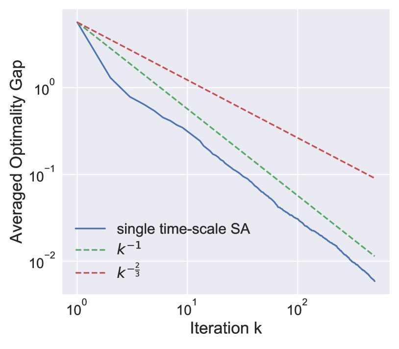
Figure 1: Solving (1) via double-sequence nonlinear SA (2). The single time-scale nonlinear SA converges with rate $\mathcal{O}(k^{-1})$, which is faster than the theoretical $\mathcal{O}(k^{-\frac{2}{3}})$ rate in (Doan, 2021).

Experiment. We first conduct an experiment to examine the possibility. Figure 1 shows the performance of using the double-sequence SA (2) to solve the following problem

$$\max_{x\in\mathbb{R}} ~{}~{}~{}-\frac{1}{2}\Big{(}x^{2}+\frac{1}{1+e^{-y^{*}(x)}}\Big{)}$$

$${\rm s.t.}~{}~{}y^{*}(x)=\arg\min_{y\in\mathbb{R}}\frac{1}{2}(y-x)^{2}.$$ (3)

We use the double-sequence SA (2) to solve (1), where

$$v(x,y)=-x-\frac{e^{-y}}{(1+e^{-y})^{2}},~{}~{}~{}h(x,y)=x-y$$ (4)

and $\zeta_{k}$, $\xi_{k}$ are independent Gaussian random variables with zero mean and standard deviations of $0.15$. It is easy to check that (4) satisfies the assumptions in the existing TTS-SA analysis (Doan, 2021). Therefore, we can use the two time-scale step sizes and achieve the iteration complexity of $\mathcal{O}(\epsilon^{-1.5})$. However, as suggested by Figure 1, the iterates still converge with step sizes in a single time-scale ($\alpha_{k}=\Theta(\frac{1}{k})$, $\beta_{k}=\Theta(\frac{1}{k})$). In this case, the iteration complexity is $\mathcal{O}(\epsilon^{-1})$, which is the same as that of double-sequence linear SA (Kaledin et al., 2020). This suggests that existing analysis of double-sequence SA might not be tight, at least for the class of updates similar to (4). Indeed, as we will show later, the iterates generated by (4) will converge with the iteration complexity of $\mathcal{O}(\epsilon^{-1})$.

	General result		Application to SBO				Application to multi-level SCO
	​​​​Ours​​​​	​​​​TTS SA ​​​​	​​​​ Ours ​​​​	​​​​​​ TTSA​​​​​​	​​​​​​​ ALSET​​​​	​​​​ ALSET-AC ​​​​	​​​​ Ours ​​​​	​​​​ $\alpha$-TSCGD ​​​​	​​​​ SG-MRL​​ ​​
​​​​SM​​​​	​​​​$\mathcal{O}(\epsilon^{-1})$​​​​	​​​​​ $\mathcal{O}(\epsilon^{-1.5})$ ​​​​​	​​​​ $\tilde{\mathcal{O}}(\epsilon^{-1})$	​​​$\tilde{\mathcal{O}}(\epsilon^{-1.5})$ ​​​​	​​​​ ~ ​​​​	​​​​ ~ ​​​​	​​​​ $\mathcal{O}(\epsilon^{-1})$ ​​​​	​​​​ $\mathcal{O}(\epsilon^{-\frac{N+5}{4}})$ ​​​​	​​​​ ~
​​​​N-SM ​​​​	$\mathcal{O}(\epsilon^{-2})$	~	​​​ $\tilde{\mathcal{O}}(\epsilon^{-2})$ ​​​	​​​ $\tilde{\mathcal{O}}(\epsilon^{-2.5})$ ​​​	​​​ $\tilde{\mathcal{O}}(\epsilon^{-2})$​​​	​​​ $\mathcal{O}(\epsilon^{-2})$​​​	​​ $\mathcal{O}(\epsilon^{-2})$	​​$\mathcal{O}(\epsilon^{-\frac{N+8}{4}})$	​​ $\mathcal{O}(\epsilon^{-4})$
​​​​Merit ​​​​	​​​​ ~ ​​​​	​​​​ Rate $\uparrow$ ​​​​	​​​​ ~ ​​​​	​​​​ Rate $\uparrow$ ​​​​	​​​​ Relax ​​​​	​​​​ Relax ​​​​	​​​​ ~ ​​​​	​​​​ Rate $\uparrow$	Rate $\uparrow$

Table 1: Comparisons with TTS SA (Doan, 2021), TTSA (Hong et al., 2020), ALSET and ALSET-AC (Chen et al., 2021b), $\alpha$-TSCGD (Yang et al., 2018a) and SG-MRL (Fallah et al., 2021). Strongly-monotone (SM) and non-strongly-monotone (N-SM) respectively represents the case where the main sequence has strongly-monotone and non-strongly-monotone increments. Rows of SM/N-SM are for the complexity and the row of Merit is for the improvements of this work over the existing work (“Rate $\uparrow$” stands for faster rate; “Relax” for relaxed assumptions).

Furthermore, existing works on TTS SA mainly focus on the double-sequence case. While in cases such as the multi-level stochastic optimization; see e.g., (Yang et al., 2018a; Sato et al., 2021), more than two sequences are involved. This necessitates the use of the multi-sequence SA. Specifically, with mappings $v:\mathbb{R}^{d_{0}}\times\mathbb{R}^{d_{1}}\dots\times\mathbb{R}^{d_{N}}\mapsto\mathbb{R}^{d_{0}}$, $h^{n}:\mathbb{R}^{d_{n-1}}\times\mathbb{R}^{d_{n}}\mapsto\mathbb{R}^{d_{n}}$, we consider the following multi-sequence Single-Timescale SA (STSA) update in this work:

where $\alpha_{k},\beta_{k,1},...,\beta_{k,N}$ are the step sizes, and $\xi_{k},\psi_{k}^{1},\dots,\psi_{k}^{N}$ are random variables. For conciseness, we have used $y_{k}^{0}\coloneqq x_{k}$ here. We call the update (5) a single-timescale update since we will show the two sequences are updated in the same time scale; that is $\lim_{k\rightarrow\infty}\alpha_{k}/\beta_{k}=c$ for some constant $c>0$. Our goal is to find the unique fixed-points $x^{*},y^{1,*},\dots,y^{N,*}$ such that

$$v(x^{*},y^{1,*},\dots,y^{N,*})=h^{1}(x^{*},y^{1,*})=\dots=h^{N}(y^{N-1,*},y^{N,*})=0.$$ (6)

Observing that in (5), for every $n$, the sequence of $y_{k}^{n}$ is coupled with that of $y_{k}^{n-1}$ and is ultimately coupled with the main sequence $x_{k}$. Meanwhile, the update of $x_{k}$ also depends on $\{y_{k}^{n}\}_{n=1}^{N}$. Since all sequences in (5) are coupled, (5) is more challenging to analyze than the double-sequence SA.

Prior art related to multi-sequence SA. The multilevel optimization problem (Sato et al., 2021) and the multilevel SCO problem (Balasubramanian et al., 2022; Xiao et al., 2022; Zhang and Xiao, 2021; Ruszczynski, 2021; Zhang and Lan, 2020) are closely related to the multi-sequence SA. To tackle the multi-level structure, these recent advances have modified the vanilla multi-sequence SA update to achieve the state-of-the-art complexity and thus their updates are not exactly in the form of (5). In particular, the recent work Sato et al. (2021) mainly focuses on the deterministic multilevel optimization, where it approximates the desired increment of $x$ by a nested algorithm, and thus its update is not in the form of (5). In contrast, we focus on the multi-sequence STSA update in (5). To the best of our knowledge, the only analysis for the exact update (5) is (Yang et al., 2018a), where the TTS technique is generalized to multi-time-scale. However, in (Yang et al., 2018a), the iteration complexity will get worse as the number of sequences $N$ increases.

This gives rise to another interesting question:

Q2: Is it possible to establish convergence rate of the update (5) that is independent of $N$?

In this work, we give affirmative answers to both Questions Q1 and Q2.

Our contributions. By exploiting the smooth assumption of the fixed points that can be satisfied in many applications, we show that the vanilla nonlinear STSA can run in a single time scale! We further prove that the order of the convergence rate is independent of the number of sequences $N$. Intuitively, this is possible because when the fixed point $y^{n,*}$ is smooth in $x$, the $y_{k}^{n}$-update converges fast enough such that its fixed-point residual after one update is at the same order as the drift of $y^{n,*}$.

In the context of prior art, our contributions can be summarized as follows (see Table 1).

C1) Single-timescale analysis for multi-sequence SA. Different from existing two-timescale analysis (Mokkadem and Pelletier, 2006; Borkar and Konda, 1997), we establish a unifying Single-Timescale analysis for SA with multiple coupled sequences that we term STSA. When all the sequences have strongly-monotone increments, we improve the $\mathcal{O}(\epsilon^{-1.5})$ iteration complexity for multi-sequence TTS-SA in (Doan, 2021) to $\mathcal{O}(\epsilon^{-1})$. When all but the main sequence have strongly monotone increments, we provide the $\mathcal{O}(\epsilon^{-2})$ iteration complexity.

C2) STSA for stochastic bilevel optimization (SBO). When applying our generic results to the SBO problem with double-sequence SA, for strongly-concave objective functions, we improve the best-known sample complexity $\tilde{\mathcal{O}}(\epsilon^{-1.5})$ of TTSA in (Hong et al., 2020) to $\tilde{\mathcal{O}}(\epsilon^{-1})$. For the non-concave objective function, we achieve the same sample complexity $\mathcal{O}(\epsilon^{-2})$ of ALSET while relaxing the bounded upper-level gradient assumption made in (Chen et al., 2021b).

C3) STSA for stochastic compositional optimization (SCO). When applying our results to the multi-level SCO problems, we improve the level-dependent sample complexities $\mathcal{O}(\epsilon^{-\frac{N+5}{4}})$ and $\mathcal{O}(\epsilon^{-\frac{N+8}{4}})$ of multi-sequence SA based $\alpha$-TSCGD method in (Yang et al., 2018a) to the level-independent iteration complexities $\tilde{\mathcal{O}}(\epsilon^{-1})$ and $\mathcal{O}(\epsilon^{-2})$, under the strongly-concave and non-concave objective functions, respectively.

C4) STSA for policy optimization in RL problems. Moreover, applying our results to the actor-critic method achieves the same $\mathcal{O}(\epsilon^{-2})$ sample complexity of ALSET-AC in (Chen et al., 2021b) while relaxing the unverifiable assumption on the stationary distribution of Markov chains; applying our results to the meta policy gradient improves the $\mathcal{O}(\epsilon^{-4})$ sample complexity of SG-MRL in (Fallah et al., 2021) to $\mathcal{O}(\epsilon^{-2})$.

Roadmap. We organize the results as follows. With the multi-sequence SA update introduced in this section, we first present our main results in Section 2. In Section 3, we apply our results to the SBO problem which also encompasses the actor-critic method. In Section 4, we apply our result to the SCO problem which also encompasses the model-agnostic meta policy gradient method.

2 Main Results: Convergence of Single-timescale Multi-sequence SA

Before introducing the main results, we will first make some standard assumptions. Throughout the discussion, we define $[N]\coloneqq\{1,2,...,N\}$, $[K]\coloneqq\{1,2,...,K\}$ and $y^{0}\coloneqq x$ for conciseness.

Assumption 1 (Smoothness of the fixed points)

For any $n\in[N]$ and $y^{n-1}\in\mathbb{R}^{d_{n-1}}$, there exists a unique $y^{n,*}(y^{n-1})\in\mathbb{R}^{d_{n}}$ such that $h^{n}(y^{n-1},y^{n,*}(y^{n-1}))=0$. Moreover, there exist constants $L_{y,n}$ and $L_{y^{\prime},n}$ such that for any $y^{n-1},\bar{y}^{n-1}\in\mathbb{R}^{d_{n-1}}$, the following inequalities hold

$$\|y^{n,*}(y^{n-1})-y^{n,*}(\bar{y}^{n-1})\| \leq L_{y,n}\|y^{n-1}-\bar{y}^{n-1}\|,$$ (7a)

$$\|\nabla y^{n,*}(y^{n-1})-\nabla y^{n,*}(\bar{y}^{n-1})\| \leq L_{y^{\prime},n}\|y^{n-1}-\bar{y}^{n-1}\|.$$ (7b)

Due to the change of $y_{k}^{n-1}$ at each iteration, the solution of $h^{n}(y_{k}^{n-1},y^{n})=0$ with respect to (w.r.t.) $y^{n}$, that is $y^{n,*}(y_{k}^{n-1})$, is drifting over consecutive iterations. Given $y_{k}^{n-1}$, since only one-step of $y_{k}^{n}$ update is performed at each iteration, one can only hope to establish convergence of $y_{k}^{n}$ if the drift of its optimal solution is controlled in some sense. Assumption 1 ensures both the zeroth-order and first-order drifts are controlled in the same scale of the change of $y_{k}^{n-1}$. This assumption is satisfied in linear SA (Kaledin et al., 2020) and other applications which will be shown later.

Define $v(x)\coloneqq v\big{(}x,y^{1,*}(x),y^{2,*}(y^{1,*}(x)),\dots,y^{N,*}(\dots y^{2,*}(y^{1,*}(x))\dots)\big{)}$. With $y^{1:N}$ as a concise notation for $(y^{1},...,y^{N})$, we make the following assumption.

Assumption 2 (Lipschitz continuity of increments)

For any $n\in[N]$, $x,\bar{x}\in\mathbb{R}^{d_{0}}$ and $y^{n},\bar{y}^{n}\in\mathbb{R}^{d_{n}}$, there exist constants $L_{v}$, $L_{v,y}$ and $L_{h,n}$ such that the following inequalities hold

$$\|v(x)-v(\bar{x})\| \!\leq\!L_{v}\|x-\bar{x}\|,$$ (8a)

$$\|v(x,y^{1:N})\!-\!v(x,\bar{y}^{1:N})\| \!\leq\!L_{v,y}\!\sum_{n=1}^{N}\!\|y^{n}\!-\!\bar{y}^{n}\|,\!$$ (8b)

$$\|h^{n}(y^{n-1},y^{n})\!-\!h^{n}(y^{n-1},\bar{y}^{n})\| \!\leq\!L_{h,n}\|y^{n}-\bar{y}^{n}\|.$$ (8c)

Define $\mathcal{F}_{k}$ as the $\sigma$-algebra generated by the random variables in $\{x_{i},y_{i}^{1:N}\}_{i=1}^{k}$ and $\mathcal{F}_{k}^{n}$ as the $\sigma$-algebra generated by $\{x_{i},y_{i}^{1:N}\}_{i=1}^{k}\cup\{y_{k+1}^{n}\}$. We make the following assumption on the noises.

Assumption 3 (Bias and variance)

There exist constants $\{c_{n},\sigma_{n}\}_{n=0}^{N}$ such that $\forall k,n$, $\|\mathbb{E}[\xi_{k}|\mathcal{F}_{k}^{1}]\|^{2}\leq c_{0}^{2}\alpha_{k}$ and $\|\mathbb{E}[\psi_{k}^{n}|\mathcal{F}_{k}^{n+1}]\|^{2}\leq c_{n}^{2}\beta_{k,n}$; $\mathbb{E}[\|\xi_{k}\|^{2}|\mathcal{F}_{k}^{1}]\leq\sigma_{0}^{2}$ and $\mathbb{E}[\|\psi_{k}^{n}\||\mathcal{F}_{k}^{n+1}]\leq\sigma_{n}^{2}$.

Here we define $\mathcal{F}_{k}^{N+1}\coloneqq\mathcal{F}_{k}$. Assumption 3 is a generalized version of the standard zero-mean noise with bounded moments assumption (Konda and Tsitsiklis, 2004). Given $\mathcal{F}_{k}$, if $\psi_{k}^{n}$ and $\xi_{k}$ are independent of each other and have zero-mean, Assumption 3 holds with $c_{n}=0$ for any $n$.

Assumption 4 (Monotonicity of $h$)

For $n\in[N]$, $h^{n}(y^{n-1},y^{n})$ is one-point strongly monotone on $y^{n,*}(y^{n-1})$ given any $y^{n-1}$; that is, there exists constant $\lambda_{n}>0$ such that (cf. $h^{n}(y^{n-1},y^{n,*})=0$)

$$\big{\langle}y^{n}\!-\!y^{n,*}(y^{n-1}),h^{n}(y^{n-1},y^{n})\big{\rangle}\leq-\lambda_{n}\|y^{n}\!-\!y^{n,*}(y^{n-1})\|^{2}.$$ (9)

Assumption 4 is implied by the standard regularity assumptions in the previous works on TTS linear SA (Konda and Tsitsiklis, 2004; Kaledin et al., 2020), and has also been exploited in the TTS nonlinear SA works; see e.g., (Mokkadem and Pelletier, 2006; Doan, 2021).

2.1 The strongly-monotone case

We first consider the case when the main sequence $x_{k}$ has strongly-monotone increment.

Assumption 5 (Monotonicity of $v$)

Suppose $v(x)$ is one-point strongly monotone on $x^{*}$; that is, there exists a positive constant $\lambda_{0}$ such that (cf. $v(x^{*})=0$)

$$\big{\langle}x-x^{*},v(x)\big{\rangle}\leq-\lambda_{0}\|x-x^{*}\|^{2}.$$ (10)

Same as Assumption 4, Assumption 5 is standard in the previous works on TTS SA (Mokkadem and Pelletier, 2006; Doan, 2021). This assumption is a regularity assumption in the case of TTS linear SA; see e.g., (Konda and Tsitsiklis, 2004, Assumption 2.3). Or in the case of bilevel optimization which will be discussed later, this assumption is satisfied when the objective function is strongly-concave.

Due to space limitation, we directly present the result below and defer the proof to Appendix B.

It is worth noting that with (7a), Theorem 1 also implies the same convergence result for the error metric $\|x_{k}-x^{*}\|^{2}+\sum_{n=1}^{N}\|y_{k}^{n}-y^{n,*}\|^{2}$, the formal justification of which is deferred to the proof of Theorem 1. In addition, the order of convergence rate in Theorem 1 is independent of $N$, which is in contrast to the convergence rate that gets worse as $N$ increases (Doan, 2021; Yang et al., 2018a).

Remark 1 (Comparison with prior art in multi-sequence SA)

Theorem 1 fills the gap between the convergence rate of double-sequence linear SA and that of double-sequence nonlinear SA by improving over the $\mathcal{O}(k^{-\frac{2}{3}})$ rate shown in (Doan, 2021). While this is done under the additional assumption (7b), as will be shown later, this assumption is satisfied in various applications. Theorem 1 also generalizes the $\mathcal{O}(\frac{1}{k})$ convergence rate in the double-sequence linear SA analysis (e.g., (Kaledin et al., 2020)) to the multi-sequence nonlinear SA case.

2.2 The non-strongly-monotone case

Some applications of multi-sequence nonlinear SA such as the actor-critic method (Konda, 2002), Assumption 5 does not hold. This motivates us to consider a more general setting in this subsection where $v(x)$ is non-strongly-monotone.

Throughout this subsection, we make the following assumption.

Assumption 6

Suppose there exists a mapping $F:\mathbb{R}^{d_{0}}\mapsto\mathbb{R}$ such that $\nabla F(x)=v(x)$. The sequence of $\{x_{k}\}$ is contained in an open set over which $F(x)$ is upper bounded; e.g., $F(x)\leq C_{F}$.

Assumption 6 is standard in SA; see e.g., (Karimi et al., 2019). As will be shown later, $F(x)$ can be chosen as the objective function when applying SA to maximization problems.

The following theorem gives the general finite-time convergence result of the nonlinear SA when the main sequence has the non-strongly-monotone increment. The proof is deferred to Appendix C.

Theorem 2 implies a finite-time convergence rate of $\mathcal{O}(K^{-2})$, which is independent of the number of sequences $N$. The error metric $\|\nabla F(x_{k})\|$ used in Theorem 2 is of interest since it is a general measure of the convergence of $x_{k}$ widely adopted in many applications of SA, especially when the increment of $x_{k}$ is not strongly-monotone. Moreover, although we have assumed the existence and uniqueness of $x^{*}$ in (6), the proof of Theorem 2 does not utilize this fact and thus the theorem applies to the more general case where $x^{*}$ is not unique or even does not exist.

Given the generic results in Theorems 1 and 2, next we will showcase that many existing SA-type algorithms for stochastic optimization and RL problems indeed satisfy either Assumptions 1–5 or Assumptions 1–4 and 6, and therefore, their convergence results can be automatically deduced from the generic STSA results in Theorems 1 and 2.

3 Application to the stochastic bilevel optimization method

In this section, we apply our generic STSA results to the stochastic bilevel optimization problems and its applications to the actor-critic algorithm in RL.

With mappings $f:\mathbb{R}^{d_{0}}\times\mathbb{R}^{d_{1}}\mapsto\mathbb{R}$ and $g:\mathbb{R}^{d_{0}}\times\mathbb{R}^{d_{1}}\mapsto\mathbb{R}$, consider the following formulation of the bilevel optimization problem:

$$\max_{x\in\mathbb{R}^{d_{0}}}F(x) \coloneqq f(x,y^{*}(x))\coloneqq\mathbb{E}_{\zeta}\big{[}f(x,y^{*}(x);\zeta)\big{]}$$ (14a)

$${\rm s.t.}~{}y^{*}(x) \coloneqq\arg\min_{y\in\mathbb{R}^{d_{1}}}g(x,y)\coloneqq\mathbb{E}_{\varphi}\big{[}g(x,y;\varphi)\big{]}$$ (14b)

where $\zeta$ and $\varphi$ are two random variables.

3.1 Reduction from the generic results

A popular approach to solving (14) is the gradient-based method (Ghadimi and Wang, 2018; Hong et al., 2020; Chen et al., 2021b). Under some conditions that will be specified later, it has been shown in (Ghadimi and Wang, 2018) that the gradient of $F(x)$ takes the following form:

$$\nabla F(x)=\nabla_{x}f(x,y^{*}(x))-\nabla_{xy}^{2}g(x,y^{*}(x))[\nabla_{yy}^{2}g(x,y^{*}(x))]^{-1}\nabla_{y}f(x,y^{*}(x)).$$ (15)

Note that here $\nabla_{x}f(x,y^{*}(x))=\frac{\partial f(x,y)}{\partial x}|_{y=y^{*}(x)}$, $\nabla_{xy}^{2}g(x,y^{*}(x))=\frac{\partial g(x,y)}{\partial x\partial y}|_{y=y^{*}(x)}$ and the same thing applies to $\nabla_{y}f(x,y^{*}(x))$ and $\nabla_{yy}^{2}g(x,y^{*}(x))$. It is clear that computing (15) requires $y^{*}(x)$, which is often unknown in practice. Instead, one can iteratively update $y_{k}$ to approach $y^{*}(x_{k})$ while using $y_{k}$ in place of $y^{*}(x_{k})$ during the computation of (15) (Hong et al., 2020; Chen et al., 2021b). This leads to an update same as that in (5) with $N\!=\!1$, where the generic mapping is defined as

$$h(x,y) =-\nabla_{y}g(x,y),$$ (16a)

$$\psi_{k} \!=\!-h(x_{k},y_{k})\!-\!\nabla_{y}g(x_{k},y_{k};\varphi_{k}),$$ (16b)

$$v(x,y) =\nabla_{x}f(x,y)-\nabla_{xy}^{2}g(x,y)[\nabla_{yy}g(x,y)]^{-1}\nabla_{y}f(x,y),$$ (16c)

$$\xi_{k} =-v(x_{k},y_{k})+\nabla_{x}f(x_{k},y_{k};\zeta_{k})-\nabla_{xy}^{2}g(x_{k},y_{k};\varphi_{k}^{\prime})H^{yy}_{k}\nabla_{y}f(x_{k},y_{k};\zeta_{k}).$$ (16d)

Since here we only have two sequences, that is $N\!=\!1$, we omit the index $n$ to simplify notations. In (16), $\zeta_{k}$ is a random variable with the same distribution as that of $\zeta$, and $\varphi_{k}$, $\varphi_{k}^{\prime}$ have the same distribution as that of $\varphi$. Here $H_{k}^{yy}$ is a stochastic approximation of the Hessian inverse $[\nabla_{yy}g(x_{k},y_{k})]^{-1}$. Given $x_{k}$, when $y_{k}$ reaches the optimal solution $y^{*}(x_{k})$, it follows from (15) that $v(x_{k},y^{*}(x_{k}))=\nabla F(x_{k})$.

As being discussed below Assumption 1, the lower-level optimal solution $y^{*}(x_{k})$ is drifting at each iteration. Under the Lipschitz continuity assumption of $y^{*}(x)$, the drifting $\|y^{*}(x_{k+1})-y^{*}(x_{k})\|$ scales with $\|x_{k+1}-x_{k}\|$ which ultimately scales with $\|\nabla F(x_{k})\|$. To control the drift scale, former analysis heavily relies on the condition that $\|\nabla F(x_{k})\|$ is bounded for any $k$. In SBO, this means to either make a strong assumption on the Lipschitz continuity of $f(x,y)$ w.r.t. $(x,y)$, which leads to the Lipschitz continuity of $F(x)$ and the boundedness of $\|\nabla F(x_{k})\|$ (Chen et al., 2021b); or to introduce projection in (16) to confine $x_{k}$ in a compact set (Hong et al., 2020), all of which greatly narrow the range of application. We will show that neither of these the conditions is not needed by applying our generic results to SBO.

Lemma 1 (Verifying assumptions of STSA)

Consider the following conditions

1. For any $x\in\mathbb{R}^{d_{1}}$, $g(x,y)$ is strongly convex w.r.t. $y$ with modulus $\lambda_{1}>0$.

2. There exist constants $L_{xy},l_{xy},l_{yy}$ such that $\nabla_{y}g(x,y)$ is $L_{xy}$-Lipschitz continuous w.r.t. x; $\nabla_{y}g(x,y)$ is $L_{h}$-Lipschitz continuous w.r.t. $y$. $\nabla_{xy}g(x,y)$, $\nabla_{yy}g(x,y)$ are respectively $l_{xy}$-Lipschitz and $l_{yy}$-Lipschitz continuous w.r.t. $(x,y)$.

3. There exist constants $l_{fx},l_{fy},l_{fy}^{\prime},l_{y}$ such that $\nabla_{x}f(x,y)$ and $\nabla_{y}f(x,y)$ are respectively $l_{fx}$ and $l_{fy}$ Lipschitz continuous w.r.t. $y$; $\nabla_{y}f(x,y)$ is $l_{fy}^{\prime}$-Lipschitz continuous w.r.t. $x$; $f(x,y)$ is $l_{y}$-Lipschitz continuous w.r.t. $y$.

4. $F(x)$ satisfies the restricted secant inequality: There exists a constant $\lambda_{0}>0$ such that $\langle\nabla F(x),x-x^{*}\rangle\leq-\lambda_{0}\|x-x^{*}\|^{2}$, where $x^{*}\coloneqq\arg\max_{x\in\mathbb{R}^{d_{1}}}F(x)$.

5. For any $k$, there exist constants $c_{0},c_{1}$ such that $\|\mathbb{E}[\xi_{k}|\mathcal{F}_{k}^{1}]\|^{2}\leq c_{0}^{2}\alpha_{k}$ and $\|\mathbb{E}[\psi_{k}|\mathcal{F}_{k}]\|^{2}\leq c_{1}^{2}\beta_{k}$. Additionally, there exist constants $\sigma_{0},\sigma_{1}$ such that $\mathbb{E}[\|\xi_{k}\|^{2}|\mathcal{F}_{k}^{1}]\leq\sigma_{0}^{2}$ and $\mathbb{E}[\|\psi_{k}\|^{2}|\mathcal{F}_{k}]\leq\sigma_{1}^{2}$.

6. There exists a constant $C_{F}$ such that $F(x)\leq C_{F}$.

We use $a\xrightarrow[]{}b$ to indicate that $a$ is a sufficient condition of $b$. Then we have

$$\ref{item:strong convex}~{}\textit{and}~{}\ref{item:g lip 2}\xrightarrow[]{}\textit{ Assumption \ref{assumption:y*}};~{}~{}\ref{item:strong convex}-\ref{item:f lip}\xrightarrow[]{}\textit{ Assumption \ref{assumption:vglip}};~{}~{}\ref{item:noise bilevel}\xrightarrow[]{}\textit{Assumption \ref{assumption:noise}};$$

$$\ref{item:strong convex}\xrightarrow[]{}\textit{ Assumption \ref{assumption:strongly g}};~{}~{}\ref{item:F RSI}\xrightarrow[]{}\textit{ Assumption \ref{assumption:strongly v}};~{}~{}\ref{item:F}\xrightarrow[]{}\textit{ Assumption \ref{assumption:integral}}.$$ (17)

The conditions listed above are standard in the literature (Ghadimi and Wang, 2018; Hong et al., 2020; Chen et al., 2021b). It is worth noting that Lemma 1 does not need the $L_{xy}$-Lipschitz continuity condition of $f(x,y)$ w.r.t. $(x,y)$. This Lipschitz condition, along with the $L_{y}$-Lipschitz continuity of $y^{*}(x)$ implied by the conditions in Lemma 1, further leads to the Lipschitz continuity of $F(x)$:

$$|F(x)-F(x^{\prime})|\leq L_{xy}(\|x-x^{\prime}\|+\|y^{*}(x)-y^{*}(x^{\prime})\|)\leq L_{xy}(L_{y}+1)\|x-x^{\prime}\|.$$ (18)

Although it is rather restrictive, this condition has been used in the previous work when $F(x)$ is not strongly-concave/convex. Lastly, condition (e) can be guaranteed by using (Ghadimi and Wang, 2018, Algorithm 3) to obtain a good enough $H_{k}^{yy}$, which requires extra $\Omega(\log\epsilon^{-1})$ samples per iteration. With Lemma 1, we have the following corollary regarding the convergence of (16).

Corollary 1 (STSA for SBO)

Consider the STSA sequences with the update in (16). Under Conditions (a)–(e), Theorem 1 holds; that is, with $\alpha_{k}=\Theta(\frac{1}{k})$ and $\beta_{k}=\Theta(\frac{1}{k})$ we have

$$\mathbb{E}\|x_{k}-x^{*}\|^{2}+\mathbb{E}\|y_{k}-y^{*}(x_{k})\|^{2}\!=\!\mathcal{O}\Big{(}\frac{1}{k}\Big{)},$$ (19a)

$$\lim_{k\xrightarrow[]{}\infty}\|x_{k}-x^{*}\|^{2}=0~{}~{}~{}{\rm and}~{}~{}~{}\lim_{k\xrightarrow[]{}\infty}\|y_{k}-y^{*}(x_{k})\|^{2}=0~{}~{}a.s.$$ (19b)

Under Conditions (a)–(c), (e) and (f), Theorem 2 holds; i.e., with $\alpha_{k}\!=\!\Theta(\frac{1}{\sqrt{K}})$, $\beta_{k}\!=\!\Theta(\frac{1}{\sqrt{K}})$, we have

$$\frac{1}{K}\sum_{k=1}^{K}\Big{(}\mathbb{E}\|\nabla F(x_{k})\|^{2}+\mathbb{E}\|y_{k}-y^{*}(x_{k})\|^{2}\Big{)}=\mathcal{O}\Big{(}\frac{1}{\sqrt{K}}\Big{)}.$$ (20)

Remark 2 (Comparison with prior art in single-loop SBO)

If $F(x)$ is strongly concave, Corollary 1 implies the sample complexity of $\mathcal{O}(\epsilon^{-1}\!\log\epsilon^{-1})$, which improves over the best-known sample complexity $\mathcal{O}(\epsilon^{-1.5}\log\epsilon^{-1})$ in (Hong et al., 2020). Different from (Hong et al., 2020), we do not need the projection of $x_{k}$ to a compact set. When $F(x)$ is non-concave, corollary 1 suggests a sample complexity of $\mathcal{O}(\epsilon^{-2}\log\epsilon^{-1})$, which is the same as the state-of-art complexity established in (Chen et al., 2021b). Corollary 1 improves the result in (Chen et al., 2021b) in two major aspects: 1) By carefully utilizing the smoothness of $y^{*}(x)$, we avoid directly bounding the term $\|x_{k+1}-x_{k}\|^{2}$ in the proof, which was originally bounded using the bounded gradient assumption in (Chen et al., 2021b). Thus we relax the Lipschitz continuity assumption on $f(x,y)$ on $x$; and, 2) An alternating update is adopted in (Chen et al., 2021b) to ensure stability, while some applications of SBO only allow simultaneous updates. Corollary 1 applies to those cases and thus has a broader range of application.

3.2 Application to advantage actor-critic

The advantage actor-critic (AC) is one of the most celebrated methods in RL. We will apply our new nonlinear SA results to AC by starting with the basic concepts in RL.

RL problems are often modeled as a MDP described by $\mathcal{M}=\{\mathcal{S},\mathcal{A},\mathcal{P},r,\gamma\}$, where $\mathcal{S}$ is the state space, $\mathcal{A}$ is the action space; $\mathcal{P}(s^{\prime}|s,a)$ is the probability of transitioning to $s^{\prime}\in\mathcal{S}$ given $(s,a)\!\in\!\mathcal{S}\!\times\!\mathcal{A}$; $r(s,a)\in[0,1]$ is the reward associated with $(s,a)$; and $\gamma\in(0,1)$ is a discount factor. A policy $\pi$ maps $\mathcal{S}$ to a probability distribution over $\mathcal{A}$, and we use $\pi(a|s)$ to denote the probability of choosing $a$ under $s$. Given a policy $\pi$, we define the value functions as $V_{\pi}(s)\coloneqq\mathbb{E}_{\pi}\!\Big{[}\sum_{t=0}^{\infty}\gamma^{t}r(s_{t},a_{t})\mid s_{0}\!=\!s\Big{]}$, where $\mathbb{E}_{\pi}$ is taken over the trajectory $(s_{0},a_{0},s_{1},a_{1},\ldots)$ generated under policy $\pi$ and transition kernel $\mathcal{P}$. With $\rho$ denoting the initial state distribution, the discounted visitation distribution induced by policy $\pi$ is defined via $d_{\pi}(s,a)=(1-\gamma)\sum_{t=0}^{\infty}\gamma^{t}\mathbf{Pr}_{\pi}(s_{t}=s\mid s_{0}\sim\rho)\pi(a|s)$. To overcome the difficulty of learning a function, we parameterize the policy with $x\in\mathbb{R}^{d_{0}}$, and solve

$$\max_{x\in\mathbb{R}^{d_{0}}}~{}F(x)\coloneqq(1-\gamma)\mathbb{E}_{s\sim\rho}[V_{\pi_{x}}(s)].$$ (21)

The policy gradient method seeks to solve this optimization problem with gradient ascent (Sutton et al., 2000), which takes the following form:

$$\nabla F(x)\!=\!\mathbb{E}_{s,a\sim d_{\pi_{x}},s^{\prime}\!\sim\!\mathcal{P}}[(r(s,a)\!+\!\gamma V_{\pi_{x}}(s^{\prime})\!-\!V_{\pi_{x}}(s))\nabla\log\pi_{x}(a|s)].$$ (22)

In order to compute (22), one will need to know the value function $V_{\pi_{x}}$ which can be difficult to compute in practice. A popular method is to estimate the value function with $\hat{V}_{y}$ parameterized by $y\in\mathbb{R}^{d_{1}}$. In this work, we focus on the linear function approximation case, i.e. $\hat{V}_{y}(s)=\phi(s)^{\top}y$ where $\phi:\mathcal{S}\mapsto\mathbb{R}^{d_{1}}$ is the feature vector. We update $y$ with the temporal difference (TD) learning method (Sutton, 1988) which takes the same form as that of (5a) with $N\!=\!1$, given by

$$h(x,y) =\mathbb{E}_{s\sim\mu_{\pi_{x}},a\sim\pi_{x},s^{\prime}\sim\mathcal{P}}[\phi(s)(\gamma\phi(s^{\prime})-\phi(s))^{\top}]y+\mathbb{E}_{s\sim\mu_{\pi_{x}},a\sim\pi_{x}}[r(s,a)\phi(s)],$$

$$\psi_{k} =-h(x_{k},y_{k})+\phi(s_{k})(\gamma\phi(s_{k}^{\prime})-\phi(s_{k}))^{\top}y+r(s_{k},a_{k})\phi(s_{k})$$ (23)

where $\mu_{\pi_{x}}$ is the stationary distribution of the Markov chain induced by policy $\pi_{x}$. Sample $(s_{k},a_{k},s_{k}^{\prime})$ is returned by some sampling protocol. Under some regularity conditions, it is known that there exists a unique $y^{*}(x)$ such that $h(x,y^{*}(x))=0$ (Bhandari et al., 2018). For simplicity, we focus on the case where $V_{\pi_{x}}(s)$ is linear-realizable; that is, $V_{\pi_{x}}(s)=\hat{V}_{y^{*}(x)}(s)$ for any $s$.

With the estimated value function $\hat{V}_{y_{k}}$, we can then perform the policy gradient update by replacing $V_{\pi_{\theta}}$ with $\hat{V}_{y_{k}}$ in (22). This update is a special case of (5b) by defining

$$v(x,y) =\mathbb{E}_{s,a\sim d_{\pi_{x}},s^{\prime}\sim\mathcal{P}}[(r(s,a)\!+\!(\gamma\phi(s^{\prime})\!-\!\phi(s))^{\top}y)\nabla\log\pi_{x}(a|s)],$$ (24a)

$$\xi_{k} =-v(x_{k},y_{k})+r(\bar{s}_{k},\bar{a}_{k})+\gamma(\phi(\bar{s}_{k}^{\prime})-\phi(\bar{s}_{k}))^{\top}y_{k}\nabla\log\pi_{x_{k}}(\bar{a}_{k}|\bar{s}_{k}).$$ (24b)

With the AC update (3.2) and (24) written in the form of STSA, we next verify the assumptions of STSA. With $A_{x}\coloneqq\mathbb{E}_{s\sim\mu_{\pi_{x}},a\sim\pi_{x},s^{\prime}\sim\mathcal{P}}[\phi(s)(\gamma\phi(s^{\prime})-\phi(s))^{\top}],b_{x}\coloneqq\mathbb{E}_{s\sim\mu_{\pi_{x}},a\sim\pi_{x}}[r(s,a)\phi(s)]$, we have the following lemma.

Lemma 2 (Verifying the assumptions of STSA)

Consider the following conditions

1. For any $s\in\mathcal{S}$, $\|\phi(s)\|\leq 1$. For any $x\in\mathbb{R}^{d_{0}}$, there exists a constant $\lambda_{1}>0$ such that $\langle y-y^{\prime},A_{x}(y-y^{\prime})\rangle\leq-\lambda_{1}\|y-y^{\prime}\|^{2}$ for any $y,y^{\prime}\in\mathbb{R}^{d_{1}}$. The smallest singular value of $A_{x}$ is lower bounded by $\sigma>0$.

2. There exist constants $L_{\pi}$,$L_{\pi}^{\prime}$ and $C_{\pi}$ such that for any $s\in\mathcal{S}$ and $a\in\mathcal{A}$ and $x,x^{\prime}\in\mathbb{R}^{d_{0}}$, the following inequalities hold: i) $\|\pi_{x}(a|s)-\pi_{x^{\prime}}(a|s)\|\leq L_{\pi}\|x-x^{\prime}\|$. ii) $\|\nabla\log\pi_{x}(a|s)-\nabla\log\pi_{x^{\prime}}(a|s)\|\leq L^{\prime}_{\pi}\|x-x^{\prime}\|$. iii) $\|\nabla\log\pi_{x}(a|s)\|\leq C_{\pi}$.

3. For any $x\in\mathbb{R}^{d_{0}}$, the Markov chain induced by the policy $\pi_{x}$ and transition kernel $\mathcal{P}$ is ergodic. There exist positive constants $\kappa$ and $\rho<1$ such that

   $$\|\mathbb{P}_{\pi_{x}}(s_{t}\in\cdot|s_{0}=s,a_{0}=a)-\mu_{\pi_{x}}(\cdot)\|_{TV}\leq\kappa\rho^{t},~{}\forall(s,a)\in\mathcal{S}\times\mathcal{A}$$ (25)

   where $\mathbb{P}_{\pi_{x}}(s_{t}\in\cdot|s_{0},a_{0})$ is the probability measure of the $t$th state $s_{t}$ on the Markov chain induced by policy $\pi_{x}$ and transition kernel $\mathcal{P}$, given the initial state and action $s_{0},a_{0}$.

4. We sample by $s_{k},a_{k}\!\sim\!d_{\pi_{x}}$, $s_{k}\!\sim\!\mathcal{P}(\cdot|s_{k},a_{k})$; $\bar{s}_{k}\!\sim\!\mu_{x}$, $\bar{a}_{k}\!\sim\!\pi_{x}(\cdot|\bar{s}_{k})$, $\bar{s}_{k}^{\prime}\!\sim\!\mathcal{P}(\cdot|\bar{s}_{k},\bar{a}_{k})$.

Then we have

$$\textit{\ref{item:A ac}--\ref{item:ergodic}}\xrightarrow[]{}\textit{Assumption \ref{assumption:y*}};~{}~{}~{}\textit{\ref{item:A ac}~{}and~{}\ref{item:policy ac}}\xrightarrow[]{}\textit{Assumption \ref{assumption:vglip}~{}and~{}\ref{assumption:strongly g}};$$

$$\textit{Assumption \ref{assumption:integral} holds with bounded reward}.$$ (26)

Moreover, a slightly modified version of Assumption 3 holds under condition (o) and (r):

$$\mathbb{E}[\xi_{k}|\mathcal{F}_{k}^{1}]=0,~{}\mathbb{E}[\psi_{k}|\mathcal{F}_{k}]=0$$

$$\|\xi_{k}\|^{2}\leq\sigma_{0}^{2}+\bar{\sigma}_{0}^{2}\|y_{k}-y^{*}(x_{k})\|^{2},\|\psi_{k}\|^{2}\leq\sigma_{1}^{2}+\bar{\sigma}_{1}^{2}\|y_{k}-y^{*}(x_{k})\|^{2}$$ (27)

where $\sigma_{0}^{2}=8C_{\pi}^{2}(1+4\sigma^{-2})$, $\bar{\sigma}_{0}^{2}=32C_{\pi}^{2}$, $\sigma_{1}^{2}=32\sigma^{-2}+8$ and $\bar{\sigma}_{1}^{2}=32$.

The conditions listed above are standard in the literature (Wu et al., 2020; Chen et al., 2021b). For the AC update in (3.2) and (24), Assumption 2–4 and 6 or their sufficient conditions have been explored in the RL context by previous works (Wu et al., 2020). However, the smoothness of $y^{*}(x)$ in Assumption 1, which is the key condition leading to a faster convergence rate, has yet been proven and was directly assumed in (Chen et al., 2021b). While in the proof of Lemma 2, we provide a formal justification for the smoothness of $y^{*}(x)$. Lastly, note that Assumption 3 is modified to (2) in AC. As $y_{k}$ converges to $y^{*}(x_{k})$, (2) reduces to Assumption 3. As a result, though (2) is a special property for AC, the convergence analysis is still within the framework of STSA.

We then directly present the following theorem with the proof deferred to Appendix E.

Theorem 3

Consider the sequences generated by (3.2) and (24) for $k=[K]$. Under conditions (o)–(r), Theorem 2 holds; that is, with $\alpha_{k}\!=\!\Theta(\frac{1}{\sqrt{K}})$ and $\beta_{k}\!=\!\Theta(\frac{1}{\sqrt{K}})$, we have

$$\frac{1}{K}\sum_{k=1}^{K}\Big{(}\mathbb{E}\|\nabla F(x_{k})\|^{2}+\mathbb{E}\|y_{k}-y^{*}(x_{k})\|^{2}\Big{)}=\mathcal{O}\Big{(}\frac{1}{\sqrt{K}}\Big{)}.$$ (28)

In (Chen et al., 2021b), the projection step is adopted in the $y_{k}$ update to ensure that $\|y_{k}\|<\infty,\forall k$. Since the projection radius is unknown in practice, adopting the projection is essentially assuming that $\|y_{k}\|$ is bounded for any $k$, which is strong. Theorem 3 holds without this projection.

4 Application to the stochastic compositional optimization method

In this section, we apply our generic STSA results to the stochastic compositional optimization problems and its applications to the meta policy gradient algorithm in RL.

Define mappings $f^{n}:\mathbb{R}^{d_{n}}\mapsto\mathbb{R}^{d_{n+1}}$ for $n=0,1,...,N$ with $d_{N+1}=1$. The stochastic compositional problem can be formulated as

$$\max_{x\in\mathbb{R}^{d_{0}}}F(x) \coloneqq f^{N}(f^{N-1}(\dots f^{0}(x)\dots)$$

$${\rm with}~{}~{}~{}f^{n}(x) \coloneqq\mathbb{E}_{\zeta^{n}}[f^{n}(x;\zeta^{n})],~{}n=0,1,...,N$$ (29)

where $\zeta^{0},\zeta^{1},\dots,\zeta^{N}$ are random variables. Here we slightly overload the notation and use $f^{n}(x;\zeta^{n})$ to represent the stochastic version of the mapping.

4.1 Reduction from the generic STSA results

To solve the problem in (4), a natural scheme is to use the stochastic gradient descent method with the gradient given by

$$\nabla F(x)\!=\!\nabla f^{0}(x)\nabla f^{1}(f^{0}(x))\cdots\nabla f^{N}(f^{N-1}(\cdots f^{0}(x)\cdots))$$ (30)

where we use $\nabla f^{n}(f^{n-1}(\dots f^{0}(x)\dots))=\nabla f^{n}(x)|_{x=f^{n-1}(\dots f^{0}(x)\dots)}$. To obtain a stochastic estimator of $\nabla F(x)$, we will need to obtain the stochastic estimators for $\nabla f^{n}(f^{n-1}(...f^{0}(x)...))$ for each $n$. For example, when $n=1$, one need the estimator of $\nabla f^{1}(\mathbb{E}_{\zeta^{0}}[f^{0}(x;\zeta^{0})])$. However, due to the possible non-linearity of $\nabla f^{1}(\cdot)$, the natural candidate $\nabla f^{1}(f^{0}(x;\zeta^{0}))$ is not an unbiased estimator of $\nabla f^{1}(\mathbb{E}_{\zeta^{0}}[f^{0}(x;\zeta^{0})])$. To tackle this issue, a popular method is to directly track $\mathbb{E}_{\zeta^{n}}[f^{n}(\cdot;\zeta^{n})]$ by variable $y^{n},n=0,1,...,N$. The update takes the following form (Yang et al., 2018a):

$$y_{k+1}^{n} =y_{k}^{n}-\beta_{k,n}(y_{k}^{n}-f^{n-1}(y_{k}^{n-1};\zeta_{k}^{n-1})),~{}n\in[N]$$ (31a)

$$x_{k+1} =x_{k}+\alpha_{k}\nabla f^{0}(x_{k};\hat{\zeta}_{k}^{0})\nabla f^{1}(y_{k}^{1};\zeta_{k}^{1})\cdots\nabla f^{N}(y_{k}^{N};\zeta_{k}^{N})$$ (31b)

where $\hat{\zeta_{k}^{0}}$ and $\zeta_{k}^{0}$ have the same distribution as that of $\zeta^{0}$, and $\zeta_{k}^{1},\dots,\zeta_{k}^{N}$ have the same distributions as that of $\zeta^{1},\dots,\zeta^{N}$ respectively. When every $y_{k}^{n}$ reaches its fixed-point $y_{k}^{n,*}$, i.e. $y_{k}^{n}=y_{k}^{n,*}\coloneqq f^{n-1}(y_{k}^{n-1})$ for any $n\in[N]$, then it follows from (30) that $\nabla f^{0}(x)\nabla f^{1}(y_{k}^{1,*})\cdots\nabla f^{N}(y_{k}^{N,*})\!=\!\nabla F(x_{k})$, which indicates that the expected update direction of $x_{k}$ in (31) is $\nabla F(x_{k})$.

Therefore, the update of $y^{n}$ in (31a) is a special case of the STSA update in (5a) by defining

$$h^{n}(y^{n-1},y^{n}) =f^{n-1}(y^{n-1})-y^{n},$$ (32a)

$$\psi_{k}^{n} =-h^{n}(y_{k}^{n-1},y_{k}^{n})+f^{n-1}(y_{k}^{n-1};\zeta_{k}^{n-1})-y_{k}^{n}.$$ (32b)

Likewise, the update of $x$ in (31b) is a special case of the STSA update in (5b) by defining

$$v(x,y^{1},y^{2},\dots,y^{N}) =\nabla f^{0}(x)\nabla f^{1}(y^{1})...\nabla f^{N}(y^{N}),$$ (33a)

$$\xi_{k} \!=\!-v(x_{k},y_{k}^{1},\dots,y_{k}^{N})+\nabla f^{0}(x_{k};\hat{\zeta}_{k}^{0})\cdots\nabla f^{N}(y_{k}^{N};\zeta_{k}^{N}).$$ (33b)

Next we provide a lemma that summarizes the sufficient conditions of Assumption 1–6. The listed conditions are standard in the literature (Yang et al., 2018a; Chen et al., 2021a).

Lemma 3 (Verifying assumptions of STSA)

Consider the following conditions

1. Given any $n\in\{0,1,\dots,N\}$, there exist positive constants $L_{y,n}$ and $L_{y^{\prime},n}$ such that the mapping $f^{n}(\cdot)$ is $L_{y,n}$-Lipschitz continuous and $L_{y^{\prime},n}$-smooth.

2. Given $\mathcal{F}_{k}$, for any $n\in[N]$: $f^{n}(y_{k}^{n-1};\zeta_{k}^{n})$ and $\nabla f^{n}(y_{k}^{n-1};\zeta_{k}^{n})$ are respectively the unbiased estimators of $f^{n}(y_{k}^{n-1})$ and $\nabla f^{n}(y_{k}^{n-1})$ with bounded variance; $f^{0}(x_{k};\hat{\zeta}_{k}^{0})$ and $\nabla f^{0}(x_{k};\hat{\zeta}_{k}^{0})$ are respectively the unbiased estimators of $f^{0}(x_{k})$ and $\nabla f^{0}(x_{k})$ with bounded variance.

3. At each iteration $k$, $\hat{\zeta}_{k}^{0},\zeta_{k}^{0},\zeta_{k}^{1},\dots,\zeta_{k}^{N}$ are conditionally independent of each other given $\mathcal{F}_{k}$.

4. Function $F(x)$ satisfies the restricted secant inequality: There exists a constant $\lambda_{0}>0$ such that $\langle\nabla F(x),x-x^{*}\rangle\leq-\lambda_{0}\|x-x^{*}\|^{2}$, where $x^{*}\coloneqq\arg\max_{x\in\mathbb{R}^{d_{1}}}F(x)$.

5. There exists a constant $C_{F}$ such that $F(x)\leq C_{F}$.

We use $a\xrightarrow[]{}b$ to indicate that $a$ is a sufficient condition of $b$. Then we have

$$\ref{item:f sc}\xrightarrow[]{}\textit{Assumption \ref{assumption:y*}~{}and~{}\ref{assumption:vglip}};~{}~{}~{}\ref{item:noise sc}\textit{~{}and~{}}\ref{item:ind}\xrightarrow[]{}\textit{Assumption \ref{assumption:noise}};~{}~{}~{}\ref{item:v monotone sc}\xrightarrow[]{}\textit{Assumption {\ref{assumption:strongly v}}};$$

$$\ref{item:F sc}\xrightarrow[]{}\textit{Assumption \ref{assumption:integral}};~{}~{}~{}\textit{Assumption \ref{assumption:strongly g} holds naturally for \eqref{eq:scha}}.$$ (34)

With Lemma 3, we can directly arrive at the following corollary on the convergence of the stochastic compositional optimization method.

Corollary 2 (STSA for multi-level SCO)

Consider the STSA sequences generated by update (31). Under Conditions (g)–(j), Theorem 1 holds. Under Conditions (g)–(i) and (k), Theorem 2 holds.

Remark 3 (Comparison with prior art in single-loop SCO)

Corollary 2 establishes the sample complexity of $\mathcal{O}(\epsilon^{-1})$ for the strongly monotone case and the complexity of $\mathcal{O}(\epsilon^{-2})$ for the non-monotone case, which are both independent of $N$. This improves over the $\mathcal{O}(\epsilon^{-\frac{N+5}{4}})$ complexity for the strongly concave case and the $\mathcal{O}(\epsilon^{-\frac{N+8}{4}})$ complexity for the non-concave case shown in (Yang et al., 2018a). There are other works that establish the same complexity as that in Corollary 2, but they require modification to the basic SA update (32) to achieve acceleration; see e.g., (Chen et al., 2021a; Balasubramanian et al., 2022; Ruszczynski, 2021).

4.2 Application to model-agnostic meta policy gradient

The model-agnostic meta policy gradient (MAMPG) aims to find a good starting policy that can be generalized to new tasks in a few stochastic policy gradient steps (Finn et al., 2017; Fallah et al., 2021). In this section, we will apply the STSA result in Section 2 to MAMPG.

Consider a set of MDPs $\{\mathcal{M}_{i}\}_{i=1}^{M}$ with $\mathcal{M}_{i}=\{\mathcal{S},\mathcal{A},\mathcal{P}_{i},r_{i},\gamma\}$. The MDPs model a set of RL tasks that share the same state and action space while having different transition kernels $\mathcal{P}_{i}$ and reward functions $r_{i}$. To be better aligned with previous works (Fallah et al., 2021), instead of the infinite-horizon objective function defined in (21), we consider the finite-horizon one. Suppose the policy $\pi$ is parametrized by $x\in\mathbb{R}^{d_{0}}$, then the objective function of task $i$ is defined as

$$F_{i}(x)\coloneqq\mathbb{E}_{\zeta\sim\pi_{x}}\Big{[}\sum_{t=0}^{H}\gamma^{t}r_{i}(s_{t},a_{t})\mid\rho_{i},\mathcal{P}_{i}\Big{]}$$ (35)

where $H\in\mathbb{N}^{+}$ is the horizon, and $\mathbb{E}_{\zeta\sim\pi_{x}}$ is taken over the trajectory $\zeta\coloneqq(s_{0},a_{0},s_{1},a_{1},...,s_{H},a_{H})$ generated under the policy $\pi_{x}$, the initial distribution $\rho_{i}$ and the transition kernels $\mathcal{P}_{i}$.

The goal of MAMPG is to find an initial policy $\pi_{x}$ that can achieve good performance in new tasks by performing a few policy gradient steps. In the case where $N$ steps of gradient update are performed, the problem of finding an initial policy parameter $x$ can be formulated as

$$\max_{x\in\mathbb{R}^{d_{0}}}F(x)\coloneqq\frac{1}{M}\sum_{i=1}^{M}F_{i}(\tilde{x}_{i}^{N}(x))~{}~{}~{}{\rm with}\,\,\tilde{x}_{i}^{n+1}=\tilde{x}_{i}^{n}+\eta\nabla F_{i}(\tilde{x}_{i}^{n}),~{}n=0,1,...,N\!-\!1$$ (36)

where $x$ is the shared initial policy parameter, i.e. $\tilde{x}_{i}^{0}=x$ for any task $i$ and $\tilde{x}_{i}^{N}(x)$ is the parameter after running $N$ steps of gradient ascent with respect to $F_{i}$ starting from $x$.

Solving (36) with SCO method. The MAMPG problem in (36) can be solved by the stochastic compositional optimization method introduced before. In order to get $\nabla F(x)$, one will need $\nabla F_{i}(\tilde{x}_{i}^{N}(x))$ for each task $i$. Observe that $F_{i}(\tilde{x}_{i}^{N}(x))$ can be written as a compositional function:

$$F_{i}(\tilde{x}_{i}^{N}(x))=f_{i}^{N}(f_{i}^{N-1}(\dots f^{0}_{i}(x)\dots))~{}~{}{\rm with}~{}~{}f_{i}^{n}(x)\coloneqq x+\eta\nabla F_{i}(x),~{}n=0,...,N\!-\!1$$ (37)

where $f_{i}^{N}(x)=F_{i}(x)$. In order to approximate $\nabla F_{i}(\tilde{x}_{i}^{N}(x))$, we can follow the discussion in Section 4.1 and introduce tracking variables $y_{i}^{n}\in\mathbb{R}^{d_{0}}$ for $n\in[N]$ which are updated as follows

$$y_{k+1,i}^{n} =y_{k,i}^{n}-\beta_{k,n}(y_{k,i}^{n}-f_{i}^{n-1}(y_{k}^{n-1};\zeta_{k,i}^{n-1})),~{}n=0,1,...,N\!-\!1$$ (38)

where we define $f_{i}^{n}(\cdot;\zeta)$ as a stochastic approximation of $f_{i}^{n}(\cdot)$ with the random trajectory $\zeta$. Then we estimate $\nabla F_{i}(\tilde{x}_{i}^{N}(x))$ by $\hat{\nabla}F_{i,k}\!\coloneqq\!\nabla f_{i}^{0}(x;\hat{\zeta}_{k,i}^{0})\nabla f_{i}^{1}(y_{k,i}^{1};\zeta_{k,i}^{1})\cdots\nabla f_{i}^{N}(y_{k,i}^{N};\zeta_{k,i}^{N})$. Once we obtain $\hat{\nabla}F_{i,k}$ for each task, we update the initial policy as $x_{k+1}=x_{k}+\frac{\alpha_{k}}{M}\sum_{i=1}^{M}\hat{\nabla}F_{i,k}$.

Let $y^{n}\in\mathbb{R}^{d_{n}M}$ concatenate $y_{i}^{n}$ for $i\in[M]$, and $f^{n}(y_{k}^{n};\zeta_{k}^{n})$ concatenate $f_{i}^{n}(y_{k,i}^{n};\zeta_{k,i}^{n})$ for $i\in[M]$. We can write the MAMPG update as a special case of STSA (5) by

$$\!\!\!h^{n}(y^{n-1},y^{n}) =f^{n-1}(y^{n-1})-y^{n},~{}~{}\psi_{k}^{n}=-h^{n}(y_{k}^{n-1},y_{k}^{n})+f^{n-1}(y_{k}^{n-1};\zeta_{k}^{n-1})-y_{k}^{n},$$ (39a)

$$\!\!\!\!\!v(x,y^{1},\ldots,y^{N}) \!=\!\frac{1}{M}\sum_{i=1}^{M}\nabla f_{i}^{0}(x)\cdots\nabla f_{i}^{N}(y_{i}^{N}),~{}\xi_{k}\!=\!-v(x_{k},y_{k}^{1},\ldots,y_{k}^{N})\!+\!\frac{1}{M}\sum_{i=1}^{M}\hat{\nabla}F_{i,k}.\!$$ (39b)

With the update (39), we summarize the sufficient conditions for the assumptions of Theorem 2.

Lemma 4 (Verifying assumptions of STSA)

Consider the following conditions:

1. There exist constants $L_{\pi}$,$L_{\pi}^{\prime}$, $L_{\pi}^{\prime\prime}$ and $C_{\pi}$ such that for any $(s,a)\!\in\!\mathcal{S}\!\times\!\mathcal{A}$ and $x,x^{\prime}\!\in\!\mathbb{R}^{d_{0}}$, we have: i) $\|\pi_{x}(a|s)\!\!-\!\!\pi_{x^{\prime}}(a|s)\|\!\!\leq\!\!L_{\pi}\|x\!\!-\!\!x^{\prime}\|$; ii) $\|\nabla\log\pi_{x}(a|s)\!-\!\nabla\log\pi_{x^{\prime}}(a|s)\|\!\leq\!L^{\prime}_{\pi}\|x\!-\!x^{\prime}\|$; iii) $\|\nabla^{2}\log\pi_{x}(a|s)\!-\!\nabla^{2}\log\pi_{x^{\prime}}(a|s)\|\!\leq\!L^{\prime\prime}_{\pi}\|x\!-\!x^{\prime}\|$ and iv) $\|\nabla\log\pi_{x}(a|s)\|\!\leq\!C_{\pi}$.

2. Given $\mathcal{F}_{k}$, we have for any $n\in[N]$ and $i\in[M]$: $f_{i}^{n}(y_{k,i}^{n-1};\zeta_{k,i}^{n})$ and $\nabla f_{i}^{n}(y_{k,i}^{n};\zeta_{k,i}^{n})$ are respectively the unbiased estimators of $f_{i}^{n}(y_{k,i}^{n-1})$ and $\nabla f_{i}^{n}(y_{k,i}^{n})$ with bounded variance. Likewise, $f_{i}^{0}(x_{k};\zeta_{k,i}^{0})$ and $\nabla f_{i}^{0}(x_{k};\hat{\zeta}_{k,i}^{0})$ are respectively unbiased estimators of $f_{i}^{0}(x_{k})$ and $\nabla f_{i}^{0}(x_{k})$ with bounded variance.

3. Given $\mathcal{F}_{k}$, $\hat{\zeta}_{k,i}^{0},\zeta_{k,i}^{0},\zeta_{k,i}^{1},\dots,\zeta_{k,i}^{N}$ are conditionally independent of each other for $i\in[M]$.

We use $a\xrightarrow[]{}b$ to indicate that $a$ is a sufficient condition of $b$. Then we have

$$\ref{item:policy}\xrightarrow[]{}\textit{Assumption \ref{assumption:y*}~{}and~{} \ref{assumption:vglip}};~{}~{}~{}\ref{item:noise mampg}\textit{~{}and~{}}\ref{item:traj}\xrightarrow[]{}\textit{Assumption \ref{assumption:noise}};$$

$$\textit{Assumption \ref{assumption:strongly g} holds by plugging in \eqref{eq:mampg h}};~{}\textit{Assumption \ref{assumption:integral} holds under the bounded reward}.$$ (40)

Condition (l) is a standard assumption commonly adopted in the literature; see e.g., (Fallah et al., 2021; Agarwal et al., 2020). It is satisfied with certain popular policy parameterization such as the softmax policy. Conditions (m) and (n) can be satisfied with the certain choice of estimators and sampling protocols which we will specify in the appendix.

Theorem 4 (Complexity of MAMPG)

Consider the STSA sequences generated by the MAMPG update in (39) for $k=[K]$. We have Theorem 2 holds under conditions (l)–(n).

Theorem 4 implies a sample complexity of $\mathcal{O}(\epsilon^{-2})$ to achieve $\epsilon$-accuracy, which improves over the $\mathcal{O}(\epsilon^{-4})$ sample complexity in (Fallah et al., 2021). Moreover, Theorem 4 holds for any $N\geq 1$ in (36), while the method in (Fallah et al., 2021) only applies to the case $N=1$.

5 Conclusions

In this work, we consider the general nonlinear SA with multiple coupled sequences, and study its non-asymptotic performance. Different from the dominating two-timescale SA analysis, we are particularly interested in under which conditions, single-timescale analysis can be applied to nonlinear SA with multiple coupled sequences. When all the sequences have strongly monotone increments, we establish the iteration complexity of $\mathcal{O}(\epsilon^{-1})$. When the main sequence is not strongly-monotone, we establish the iteration complexity of $\mathcal{O}(\epsilon^{-2})$. We then apply our generic SA analysis to stochastic bilevel and compositional optimization and improve their existing results. Specifically, we improve the state-of-the-art convergence rate of: 1) the SBO method and its application to the AC method; and, 2) the multi-level SCO method and its application to the MAMPG method.

Appendix A Additional related works

In this section, we review additional prior work on the applications of multi-sequence SA.

Gradient-based stochastic bilevel optimization. One recent application of multi-sequence SA is on the stochastic gradient-based bilevel optimization. The bilevel optimization was first introduced in (Stackelberg, 1952). Recently, the gradient-based bilevel methods have gained growing popularity (Sabach and Shtern, 2017; Franceschi et al., 2018; Grazzi et al., 2020; Liu et al., 2020). The finite-time convergence of the double-loop bilevel optimization methods has been studied in some previous works; see e.g., (Ghadimi and Wang, 2018; Ji et al., 2021; Ji and Liang, 2021). Later, (Hong et al., 2020) proved the finite-time convergence rate for the single-loop two time-scale bilevel optimization method, which was then improved by (Chen et al., 2021b) to the optimal rate with additional assumptions and a more refined analysis. There are also other works that incorporate momentum to accelerate the convergence rate; see e.g., (Chen et al., 2022; Khanduri et al., 2021; Guo and Yang, 2021; Yang et al., 2021). After our initial conference submission, we have also noticed some concurrent works that are relevant to this work; e.g., (Dagreou et al., 2022; Grazzi et al., 2022; Li et al., 2022; Hu et al., 2022). Specifically, (Dagreou et al., 2022) proposed a SBO method with the variance-reduction technique and achieved optimal rate. And (Grazzi et al., 2022) proposed a SBO method that achieves the optimal rate without warm-start. The algorithms in (Dagreou et al., 2022; Grazzi et al., 2022) are not a case of the plain-vanilla SA update discussed in this work and thus its analysis is not applicable to our problem. In addition, the multi-block min-max bilevel algorithm has been studied in (Hu et al., 2022). Lastly, (Li et al., 2022) proposed a single-loop SBO method without Hessian inverse, but it required the bounded-gradient assumption not needed in this work.

Gradient-based stochastic compositional optimization. Stochastic compositional optimization algorithm is also a recent application of multi-sequence SA. The two time-scale stochastic compositional optimization method has been proposed in (Wang et al., 2017a, b). Due to the two time-scale step sizes choice, the convergence rate of (Wang et al., 2017a, b) is slower than that of the SGD. In order to improve the convergence, (Ghadimi et al., 2020; Chen et al., 2021a; Ruszczynski, 2021; Balasubramanian et al., 2022) have modified the basic update in (Wang et al., 2017a; Yang et al., 2018a) and successfully established the convergence rate same as that of SGD. Concurrent to this work, (Jiang et al., 2022) proposed a variance-reduced SCO method that achieved the optimal rate under variance-reduction, but the present work focuses on establishing an optimal rate for the SA update without having diminishing variance. Due to the difference in the update scheme, their analysis is not directly applicable to our SCO case.

Actor-critic method with linear function approximation. After its first introduction in (Konda and Borkar, 1999), the finite-sample guarantee for the AC algorithm has been established in (Yang et al., 2018b; Kumar et al., 2019; Fu et al., 2020) with i.i.d. sampling. In (Qiu et al., 2019), the finite-time convergence rate has been established for the nested-loop AC under the Markovian setting, which was later improved improved by (Xu et al., 2020). On the other hand, the finite-time convergence of two-timescale AC has been studied in (Wu et al., 2020) under Markovian sampling and (Hong et al., 2020; Chen et al., 2021b) under i.i.d. sampling. Concurrent to our work, a recent work (Olshevsky and Gharesifard, 2022) has used the small-gain theorem to analyze the single-loop AC algorithm and achieved the sample complexity with the best-known dependence on the condition number. However, (Olshevsky and Gharesifard, 2022) still requires projection in the critic update.

Appendix B Proof of Theorem 1

B.1 Analysis of the lower-level sequences

For brevity, we define the shorthand notations $y_{k}^{n,*}\coloneqq y^{n,*}(y^{n-1}_{k})$ with $y_{k}^{1,*}\coloneqq y^{1,*}(x_{k})$. Also, we write $\mathbb{E}[\cdot|\mathcal{F}_{k}]$ as $\mathbb{E}_{k}[\cdot]$ for brevity.

One-step contraction of lower-level sequences. With $y_{k}^{0}=x_{k}$, it holds for any $n\in[N]$ that

$$\mathbb{E}_{k}\|y_{k+1}^{n}\!-\!y_{k}^{n,*}\|^{2} \!=\!\|y_{k}^{n}-y_{k}^{n,*}\|^{2}\!+\!2\beta_{k,n}\mathbb{E}_{k}\langle y_{k}^{n}\!-\!y_{k}^{n,*},h^{n}(y_{k}^{n-1},y_{k}^{n})\!+\!\psi_{k}^{n}\rangle\!+\!\mathbb{E}_{k}\|y_{k+1}^{n}\!-\!y_{k}^{n}\|^{2}\!.\!$$ (41)

The second term in (41) can be bounded as

$$\mathbb{E}_{k}\langle y_{k}^{n}-y_{k}^{n,*},h^{n}(y_{k}^{n-1},y_{k}^{n})+\psi_{k}^{n}\rangle =\langle y_{k}^{n}-y_{k}^{n,*},h^{n}(y_{k}^{n-1},y_{k}^{n}))\rangle+\langle y_{k}^{n}-y_{k}^{n,*},\mathbb{E}_{k}[\psi_{k}^{n}]\rangle$$

$$\leq-\lambda_{n}\|y_{k}^{n}-y_{k}^{n,*}\|^{2}+\|y_{k}^{n}-y_{k}^{n,*}\|\|\mathbb{E}_{k}[\psi_{k}^{n}]\|$$

$$\leq-\lambda_{n}\|y_{k}^{n}-y_{k}^{n,*}\|^{2}+\frac{\lambda_{n}}{4}\|y_{k}^{n}-y_{k}^{n,*}\|^{2}+\frac{1}{\lambda_{n}}\|\mathbb{E}_{k}[\psi_{k}^{n}]\|^{2}$$

$$\leq-\frac{3\lambda_{n}}{4}\|y_{k}^{n}-y_{k}^{n,*}\|^{2}+\frac{c_{n}^{2}}{\lambda_{n}}\beta_{k,n},$$ (42)

where the first inequality follows from the strong monotonicity of $h(y^{n-1},y^{n})$ in Assumption 4, the second inequality follows from the Young’s inequality, and the last inequality follows from the bias of the increment $\psi_{k}^{n}$ in Assumption 3.

The third term in (41) can be bounded as

$$\mathbb{E}_{k}\|y_{k+1}^{n}-y_{k}^{n}\|^{2} \leq 2\beta_{k,n}^{2}\big{(}\|h^{n}(y_{k}^{n-1},y_{k}^{n})\|^{2}+\sigma_{n}^{2}\big{)}\leq 2L_{h,n}^{2}\beta_{k,n}^{2}\|y_{k}^{n}-y_{k}^{n,*}\|+2\sigma_{n}^{2}\beta_{k,n}^{2}$$ (43)

where the last inequality follows from Assumption 2 which gives

$$\|h^{n}(y_{k}^{n-1},y_{k}^{n})\|=\|h^{n}(y_{k}^{n-1},y_{k}^{n})-\underbrace{h^{n}(y_{k}^{n-1},y_{k}^{n,*}(y_{k}^{n-1}))}_{=0}\|\leq L_{h,n}\|y_{k}^{n}-y_{k}^{n,*}(y_{k}^{n-1})\|.$$ (44)

Collecting the upper bounds in (B.1) and (43) yields

$$\mathbb{E}_{k}\|y_{k+1}^{n}-y_{k}^{n,*}\|^{2} \leq(1-\frac{3}{2}\lambda_{n}\beta_{k,n}+2L_{h,n}^{2}\beta_{k,n}^{2})\|y_{k}^{n}-y_{k}^{n,*}\|^{2}+2(\sigma_{n}^{2}\!+\!c_{n}^{2}\lambda_{n}^{-1})\beta_{k,n}^{2}$$

$$\leq(1-\lambda_{n}\beta_{k,n})\|y_{k}^{n}-y_{k}^{n,*}\|^{2}+2(\sigma_{n}^{2}\!+\!c_{n}^{2}\lambda_{n}^{-1})\beta_{k,n}^{2},$$ (45)

where the last inequality is due to the choice of step size that satisfies $2L_{h,n}^{2}\beta_{k,n}^{2}\leq\frac{\lambda_{n}}{2}\beta_{k,n}$.

Bounding the drifting optimality gap. For any $n\geq 1$, we have

$$\|y_{k+1}^{n}-y_{k+1}^{n,*}\|^{2} =\|y_{k+1}^{n}-y_{k}^{n,*}\|^{2}+2\langle y_{k}^{n,*}-y_{k+1}^{n},y_{k+1}^{n,*}-y_{k}^{n,*}\rangle+\|y_{k}^{n,*}-y_{k+1}^{n,*}\|^{2}.$$ (46)

(1) When $n\geq 2$. By the mean-value theorem, for some $\hat{y}_{k+1}^{n-1}=ay_{k}^{n-1}+(1-a)y_{k+1}^{n-1},a\in[0,1]$, the second term in (46) can be rewritten as

$$\langle y_{k}^{n,*}-y_{k+1}^{n},y_{k+1}^{n,*}-y_{k}^{n,*}\rangle =\langle y_{k}^{n,*}-y_{k+1}^{n},\nabla y^{n,*}(\hat{y}_{k+1}^{n-1})^{\top}(y_{k+1}^{n-1}-y_{k}^{n-1})\rangle$$

$$=\langle y_{k}^{n,*}-y_{k+1}^{n},\beta_{k,n-1}\nabla y^{n,*}(\hat{y}_{k+1}^{n-1})^{\top}h^{n-1}(y_{k}^{n-2},y_{k}^{n-1})\rangle$$

$$\quad+\langle y_{k}^{n,*}-y_{k+1}^{n},\beta_{k,n-1}\nabla y^{n,*}(\hat{y}_{k+1}^{n-1})^{\top}\psi_{k}^{n-1}\rangle.$$ (47)

The first term in the right-hand side (RHS) of (B.1) can be bounded as

$$\langle y_{k}^{n,*}-y_{k+1}^{n},\beta_{k,n-1}\nabla y^{n,*}(\hat{y}_{k+1}^{n-1})^{\top}h^{n-1}(y_{k}^{n-2},y_{k}^{n-1})\rangle$$

$$\leq L_{y,n}\beta_{k,n-1}\|y_{k}^{n,*}-y_{k+1}^{n}\|\|h^{n-1}(y_{k}^{n-2},y_{k}^{n-1})\|$$

$$\leq L_{y,n}L_{h,n-1}\beta_{k,n-1}\|y_{k}^{n,*}-y_{k+1}^{n}\|\|y_{k}^{n-1}-y_{k}^{n-1,*}\|$$

$$\leq\frac{2L_{y,n}^{2}L_{h,n-1}^{2}}{\lambda_{n-1}}\beta_{k,n-1}\|y_{k}^{n,*}-y_{k+1}^{n}\|^{2}+\frac{\lambda_{n-1}}{8}\beta_{k,n-1}\|y_{k}^{n-1}-y_{k}^{n-1,*}\|^{2}$$ (48)

where the second inequality follows from

$$\|h^{n-1}(y_{k}^{n-2},y_{k}^{n-1})\| =\|h^{n-1}(y_{k}^{n-2},y_{k}^{n-1})-h^{n-1}(y_{k}^{n-2},y_{k}^{n-1,*})\|$$

$$\leq L_{h,n-1}\|y_{k}^{n-1}-y_{k}^{n-1,*}\|.$$ (49)

The second term in the RHS of (B.1) can be further decomposed into

$$\langle y_{k}^{n,*}-y_{k+1}^{n},\beta_{k,n-1}\nabla y^{n,*}(\hat{y}_{k+1}^{n-1})^{\top}\psi_{k}^{n-1}\rangle$$

$$=\langle y_{k}^{n,*}-y_{k+1}^{n},\beta_{k,n-1}(\nabla y^{n,*}(\hat{y}_{k+1}^{n-1})-\nabla y^{n,*}(y_{k}^{n-1}))^{\top}\psi_{k}^{n-1}\rangle$$

$$\quad+\langle y_{k}^{n,*}-y_{k+1}^{n},\beta_{k,n-1}\nabla y^{n,*}(y_{k}^{n-1})^{\top}\psi_{k}^{n-1}\rangle.$$ (50)

Taking expectation on the first term in the RHS of (B.1) leads to

$$\mathbb{E}_{k}\langle y_{k}^{n,*}-y_{k+1}^{n},\beta_{k,n-1}\big{(}\nabla y^{n,*}(\hat{y}_{k+1}^{n-1})-\nabla y^{n,*}(y_{k}^{n-1})\big{)}^{\top}\psi_{k}^{n-1}\rangle$$

$$\leq L_{y^{\prime},n}\beta_{k,n-1}\mathbb{E}_{k}\big{[}\|y_{k}^{n,*}-y_{k+1}^{n}\|\|\hat{y}_{k+1}^{n-1}-y_{k}^{n-1}\|\|\psi_{k}^{n-1}\|\big{]}$$

$$\stackrel{{\scriptstyle(a)}}{{\leq}}L_{y^{\prime},n}\beta_{k,n-1}\mathbb{E}_{k}\big{[}\|y_{k}^{n,*}-y_{k+1}^{n}\|\|y_{k+1}^{n-1}-y_{k}^{n-1}\|\|\psi_{k}^{n-1}\|\big{]}$$

$$\stackrel{{\scriptstyle(b)}}{{\leq}}L_{y^{\prime},n}\beta_{k,n-1}^{2}\Big{(}\mathbb{E}_{k}\big{[}\|y_{k}^{n,*}-y_{k+1}^{n}\|\|h^{n-1}(y_{k}^{n-2},y_{k}^{n-1})\|\|\psi_{k}^{n-1}\|\big{]}+\mathbb{E}_{k}\big{[}\|y_{k}^{n,*}-y_{k+1}^{n}\|\|\psi_{k}^{n-1}\|^{2}\big{]}\Big{)}$$

$$=L_{y^{\prime},n}\beta_{k,n-1}^{2}\Big{(}\mathbb{E}_{k}\big{[}\|y_{k}^{n,*}-y_{k+1}^{n}\|\|h^{n-1}(y_{k}^{n-2},y_{k}^{n-1})\|\mathbb{E}[\|\psi_{k}^{n-1}\||\mathcal{F}_{k}^{n}]\big{]}+\mathbb{E}_{k}\big{[}\|y_{k}^{n,*}-y_{k+1}^{n}\|\|\psi_{k}^{n-1}\|^{2}\big{]}\Big{)}$$

$$\stackrel{{\scriptstyle(c)}}{{\leq}}L_{y^{\prime},n}\beta_{k,n-1}^{2}\Big{(}\sigma_{n-1}\mathbb{E}_{k}\big{[}\|y_{k}^{n,*}-y_{k+1}^{n}\|\|h^{n-1}(y_{k}^{n-2},y_{k}^{n-1})\|\big{]}+\sigma_{n-1}^{2}\mathbb{E}_{k}\|y_{k}^{n,*}-y_{k+1}^{n}\|\Big{)}$$

$$\!\leq\!L_{y^{\prime},n}\beta_{k,n\!-\!1}^{2}\Big{(}\sigma_{n\!-\!1}\mathbb{E}_{k}\big{[}\|y_{k}^{n,*}\!-\!y_{k+1}^{n}\|\|h^{n\!-\!1}(y_{k}^{n\!-\!2},y_{k}^{n\!-\!1})\|\big{]}+\frac{\sigma_{n\!-\!1}^{2}}{2}\mathbb{E}_{k}\|y_{k}^{n,*}\!-\!y_{k+1}^{n}\|^{2}+\frac{\sigma_{n\!-\!1}^{2}}{2}\Big{)}\!\!\!$$

$$\stackrel{{\scriptstyle(d)}}{{\leq}}L_{y^{\prime},n}\sigma_{n\!-\!1}\beta_{k,n\!-\!1}^{2}\Big{(}\frac{L_{h,n\!-\!1}\!+\!\sigma_{n\!-\!1}}{2}\mathbb{E}_{k}\|y_{k+1}^{n}\!-\!y_{k}^{n,*}\|^{2}+\frac{L_{h,n\!-\!1}}{2}\|y_{k}^{n\!-\!1}\!-\!y_{k}^{n\!-\!1,*}\|^{2}+\frac{\sigma_{n\!-\!1}}{2}\Big{)},$$ (51)

where (a) is due to

$$\|\hat{y}_{k+1}^{n-1}-y_{k}^{n-1}\|=(1-a)\|y_{k}^{n-1}-y_{k+1}^{n-1}\|\leq\|y_{k}^{n-1}-y_{k+1}^{n-1}\|,$$ (52)

then (b) is due to

$$\|y_{k+1}^{n-1}-y_{k}^{n-1}\|\leq\beta_{k}^{n-1}\big{(}\|h^{n-1}(y_{k}^{n-2},y_{k}^{n-1})\|+\|\psi_{k}^{n-1}\|\big{)}$$ (53)

and (c) follows from Assumption 3 and Jensen’s inequality:

$$\mathbb{E}[\|\psi_{k}^{n}\|]=\mathbb{E}[\sqrt{\|\psi_{k}^{n}\|^{2}}]\leq\sqrt{\mathbb{E}\|\psi_{k}^{n}\|^{2}}\leq\sigma_{n},$$ (54)

the (d) follows from (B.1) and one-step Young’s inequality:

$$\|y_{k}^{n,*}\!-\!y_{k+1}^{n}\|\|h^{n\!-\!1}(y_{k}^{n\!-\!2},y_{k}^{n\!-\!1})\| \stackrel{{\scriptstyle\eqref{eq:hn-1}}}{{\leq}}L_{h,n-1}\|y_{k}^{n,*}\!-\!y_{k+1}^{n}\|\|y_{k}^{n-1}-y_{k}^{n-1,*}\|$$

$$\leq\frac{L_{h,n-1}}{2}\|y_{k}^{n,*}\!-\!y_{k+1}^{n}\|^{2}+\frac{L_{h,n-1}}{2}\|y_{k}^{n-1}-y_{k}^{n-1,*}\|^{2}.$$ (55)

The second term in (B.1) can be bounded as

$$\mathbb{E}_{k}\langle y_{k}^{n,*}-y_{k+1}^{n},\beta_{k-1,n}\nabla y^{n,*}(y_{k}^{n-1})^{\top}\psi_{k}^{n-1}\rangle =\mathbb{E}_{k}\big{[}\langle y_{k}^{n,*}-y_{k+1}^{n},\beta_{k,n-1}\nabla y^{n,*}(x_{k})^{\top}\mathbb{E}[\psi_{k}^{n-1}|\mathcal{F}_{k}^{n}]\rangle\big{]}$$

$$\leq L_{y,n}\beta_{k,n-1}\mathbb{E}_{k}[\|y_{k}^{n,*}-y_{k+1}^{n}\|\|\mathbb{E}[\psi_{k}^{n-1}|\mathcal{F}_{k}^{n}]\|]$$

$$\stackrel{{\scriptstyle(a)}}{{\leq}}\frac{L_{y,n}c_{n-1}}{2}\beta_{k,n-1}\big{(}\mathbb{E}_{k}\|y_{k}^{n,*}-y_{k+1}^{n}\|^{2}+\beta_{k,n-1}\big{)}$$ (56)

where (a) follows from Assumption 3.

Collecting and substituting the upper bounds in (B.1), (B.1) and (B.1) into (B.1) yields

$$\mathbb{E}_{k}\langle y_{k}^{n,*}-y_{k+1}^{n},y_{k+1}^{n,*}-y_{k}^{n,*}\rangle$$

$$\leq\big{(}\big{(}\frac{L_{y,n}c_{n-1}}{2}+\frac{2L_{y,n}^{2}L_{h,n-1}^{2}}{\lambda_{n-1}}\big{)}\beta_{k,n-1}+L_{y^{\prime},n}\sigma_{n-1}\frac{L_{h,n-1}\!+\!\sigma_{n-1}}{2}\beta_{k,n-1}^{2}\big{)}\mathbb{E}_{k}\|y_{k+1}^{n}-y_{k}^{n,*}\|^{2}$$

$$\quad\!+\!\big{(}\frac{\lambda_{n-1}}{8}\beta_{k,n-1}\!+\!\frac{L_{y^{\prime},n}\sigma_{n-1}L_{h,n-1}}{2}\beta_{k,n-1}^{2}\big{)}\|y_{k}^{n-1}\!-\!y_{k}^{n-1,*}\|^{2}\!+\!\frac{L_{y^{\prime},n}\sigma_{n-1}^{2}\!+\!L_{y,n}c_{n-1}}{2}\beta_{k,n-1}^{2}.$$ (57)

The last term in (46) can be bounded as

$$\mathbb{E}_{k}\|y_{k}^{n,*}-y_{k+1}^{n,*}\|^{2} \leq L_{y,n}^{2}\beta_{k,n-1}^{2}\mathbb{E}_{k}\|h^{n-1}(y_{k}^{n-2},y_{k}^{n-1})+\psi_{k}^{n-1}\|^{2}$$

$$\leq 2L_{y,n}^{2}\beta_{k,n-1}^{2}\|h^{n-1}(y_{k}^{n-2},y_{k}^{n-1})\|^{2}+2L_{y,n}^{2}\sigma_{n-1}^{2}\beta_{k,n-1}^{2}$$

$$\stackrel{{\scriptstyle\eqref{eq:hn-1}}}{{\leq}}2L_{y,n}^{2}L_{h,n-1}^{2}\beta_{k,n-1}^{2}\|y_{k}^{n-1}-y_{k}^{n-1,*}\|^{2}+2L_{y,n}^{2}\sigma_{n-1}^{2}\beta_{k,n-1}^{2}.$$ (58)

Substituting the upper bounds in (B.1) and (B.1) into (46) yields (for $2\leq\!n\leq N$)

$$\mathbb{E}_{k}\|y_{k+1}^{n}-y_{k+1}^{n,*}\|^{2}$$

$$\leq\big{(}1+\big{(}L_{y,n}c_{n-1}+\frac{4L_{y,n}^{2}L_{h,n-1}^{2}}{\lambda_{n-1}}\big{)}\beta_{k,n-1}+L_{y^{\prime},n}\sigma_{n-1}(L_{h,n-1}\!+\!\sigma_{n-1})\beta_{k,n-1}^{2}\big{)}\mathbb{E}_{k}\|y_{k+1}^{n}-y_{k}^{n,*}\|^{2}$$

$$\quad\!+\!\frac{\lambda_{n-1}}{2}\beta_{k,n-1}\|y_{k}^{n-1}\!-\!y_{k}^{n-1,*}\|^{2}\!+\!(L_{y^{\prime},n}\sigma_{n-1}^{2}\!+\!L_{y,n}c_{n-1}\!+\!2L_{y,n}^{2}\sigma_{n-1}^{2})\beta_{k,n-1}^{2}$$ (59)

where we have used the following condition of the step size to simplify the inequality:

$$(L_{y^{\prime},n}\sigma_{n-1}L_{h,n-1}+2L_{y,n}^{2}L_{h,n-1}^{2})\beta_{k,n-1}^{2}\leq\frac{\lambda_{n-1}}{4}\beta_{k,n-1},~{}~{}~{}2\leq n\leq N.$$ (60)

(2) When $n=1$. The update of $y_{k}^{1}$ is correlated with its upper level variable $x_{k}$ instead of $y_{k}^{n-1}$ when $n\!\geq\!2$. And since the update of $x_{k}$ depends on all variables while the update of $y_{k}^{n-1}~{}(n\!\geq\!2)$ only depends on $y_{k}^{n-2}$, the analysis of $y_{k}^{1}$ is different from that of $y_{k}^{n}~{}(n\!>\!2)$. The difference therefore lies in analyzing (46), which captures the dependence of lower level variable to its upper level variable.

By the mean-value theorem, for some $\hat{x}_{k+1}=ax_{k}+(1-a)x_{k+1},a\in[0,1]$, the second term in (46) can be rewritten as

$$\langle y_{k}^{1,*}-y_{k+1}^{1},y_{k+1}^{1,*}-y_{k}^{1,*}\rangle =\langle y_{k}^{1,*}-y_{k+1}^{1},\nabla y^{1,*}(\hat{x}_{k+1})^{\top}(x_{k+1}-x_{k})\rangle$$

$$=\langle y_{k}^{1,*}-y_{k+1}^{1},\alpha_{k}\nabla y^{1,*}(\hat{x}_{k+1})^{\top}v(x_{k},y_{k}^{1:N})\rangle$$

$$\quad+\langle y_{k}^{1,*}-y_{k+1}^{1},\alpha_{k}\nabla y^{1,*}(\hat{x}_{k+1})^{\top}\xi_{k}\rangle.$$ (61)

The first term in the RHS of (B.1) can be bounded as

$$\langle y_{k}^{1,*}-y_{k+1}^{1},\alpha_{k}\nabla y^{1,*}(\hat{x}_{k+1})^{\top}v(x_{k},y_{k}^{1:N})\rangle$$

$$\leq L_{y,1}\alpha_{k}\|y_{k}^{1,*}-y_{k+1}^{1}\|\|v(x_{k},y_{k}^{1:N})\|$$ (62)

$$\stackrel{{\scriptstyle(a)}}{{\leq}}L_{y,1}\alpha_{k}\big{(}L_{v,y}\|y_{k}^{1,*}-y_{k+1}^{1}\|\sum_{n=1}^{N}L_{y}(n)\|y_{k}^{n}-y_{k}^{n,*}\|+L_{v}\|y_{k}^{1,*}-y_{k+1}^{1}\|\|x_{k}-x^{*}\|\big{)}$$

$$\stackrel{{\scriptstyle(b)}}{{\leq}}L_{y,1}\alpha_{k}\big{(}\frac{L_{v,y}}{2}\|y_{k}^{1,*}\!-\!y_{k\!+\!1}^{1}\|^{2}\!+\!\frac{L_{v,y}N}{2}\sum_{n=1}^{N}L^{2}_{y}(n)\|y_{k}^{n}\!-\!y_{k}^{n,*}\|^{2}\!+\!\frac{L_{y,1}L_{v}^{2}}{\lambda_{0}}\|y_{k}^{1,*}\!-\!y_{k\!+\!1}^{1}\|^{2}\!+\!\frac{\lambda_{0}}{4L_{y,1}}\|x_{k}\!-\!x^{*}\|^{2}\big{)}$$

$$\!=\!(\frac{L_{y,1}L_{v,y}}{2}\!+\!\frac{L_{y,1}^{2}L_{v}^{2}}{\lambda_{0}})\alpha_{k}\|y_{k\!+\!1}^{1}\!-\!y_{k}^{1,*}\|^{2}\!+\!\frac{L_{y,1}L_{v,y}N}{2}\alpha_{k}\sum_{n=1}^{N}L^{2}_{y}(n)\|y_{k}^{n}\!-\!y_{k}^{n,*}\|^{2}\!+\!\frac{\lambda_{0}}{4}\alpha_{k}\|x_{k}\!-\!x^{*}\|^{2}\!$$ (63)

and (a) follows from

$$\|v(x_{k},y_{k}^{1:N})\| =\|v(x_{k},y_{k}^{1:N})-v(x_{k})+v(x_{k})-\underbrace{v(x^{*})}_{=0}\|$$

$$\leq\|v(x_{k},y_{k}^{1:N})-v(x_{k})\|+L_{v}\|x_{k}-x^{*}\|$$

$$\leq L_{v,y}\sum_{n=1}^{N}L_{y}(n)\|y_{k}^{n}-y_{k}^{n,*}\|+L_{v}\|x_{k}-x^{*}\|,$$ (64)

where the first inequality follows from Assumption 2 and the last inequality follows from Lemma 8; and (b) follows from Young’s inequality:

$$\|y_{k}^{1,*}-y_{k+1}^{1}\|\sum_{n=1}^{N}L_{y}(n)\|y_{k}^{n}-y_{k}^{n,*}\| \leq\frac{1}{2}\|y_{k}^{1,*}-y_{k+1}^{1}\|^{2}+\frac{1}{2}\big{(}\sum_{n=1}^{N}L_{y}(n)\|y_{k}^{n}-y_{k}^{n,*}\|\big{)}^{2}$$

$$\leq\frac{1}{2}\|y_{k}^{1,*}-y_{k+1}^{1}\|^{2}+\sum_{n=1}^{N}\frac{N}{2}L^{2}_{y}(n)\|y_{k}^{n}-y_{k}^{n,*}\|^{2},$$ (65a)

and

$$L_{v}\|y_{k}^{1,*}-y_{k+1}^{1}\|\|x_{k}-x^{*}\|\leq\frac{L_{y,1}L_{v}^{2}}{\lambda_{0}}\|y_{k}^{1,*}\!-\!y_{k\!+\!1}^{1}\|^{2}\!+\!\frac{\lambda_{0}}{4L_{y,1}}\|x_{k}\!-\!x^{*}\|^{2}.$$ (65b)

The second term in the RHS of (B.1) can be further decomposed as

$$\mathbb{E}_{k}\langle y_{k}^{1,*}-y_{k+1}^{1},\alpha_{k}\nabla y^{1,*}(\hat{x}_{k+1})^{\top}\xi_{k}\rangle$$

$$=\mathbb{E}_{k}\langle y_{k}^{1,*}-y_{k+1}^{1},\alpha_{k}\big{(}\nabla y^{1,*}(\hat{x}_{k+1})-\nabla y^{1,*}(x_{k})\big{)}^{\top}\xi_{k}\rangle+\mathbb{E}_{k}\langle y_{k}^{1,*}-y_{k+1}^{1},\alpha_{k}\nabla y^{1,*}(x_{k})^{\top}\xi_{k}\rangle.$$ (66)

The first term in the RHS of (B.1) can be bounded similarly to (B.1), with the upper level update term $\|x_{k+1}-x_{k}\|$ in place of $\|y_{k+1}^{n-1}-y_{k}^{n-1}\|~{}(n\!>\!2)$, that is

$$\mathbb{E}_{k}\langle y_{k}^{1,*}-y_{k+1}^{1},\alpha_{k}\big{(}\nabla y^{1,*}(\hat{x}_{k+1})-\nabla y^{1,*}(x_{k})\big{)}^{\top}\xi_{k}\rangle$$

$$=\mathbb{E}_{k}\langle y_{k}^{1,*}-y_{k+1}^{1},\alpha_{k}\big{(}\nabla y^{1,*}(\hat{x}_{k+1})-\nabla y^{1,*}(x_{k})\big{)}^{\top}\xi_{k}\rangle$$

$$\leq L_{y^{\prime},1}\alpha_{k}\mathbb{E}_{k}\big{[}\|y_{k}^{1,*}-y_{k+1}^{1}\|\|\hat{x}_{k+1}-x_{k}\|\|\xi_{k}\|\big{]}$$

$$\leq L_{y^{\prime},1}\alpha_{k}\mathbb{E}_{k}\big{[}\|y_{k}^{1,*}-y_{k+1}^{1}\|\|x_{k+1}-x_{k}\|\|\xi_{k}\|\big{]}$$

$$\leq L_{y^{\prime},1}\alpha_{k}^{2}\Big{(}\mathbb{E}_{k}\big{[}\|y_{k}^{1,*}-y_{k+1}^{1}\|\|v(x_{k},y_{k}^{1:N})\|\|\xi_{k}\|\big{]}+\mathbb{E}_{k}\big{[}\|y_{k}^{1,*}-y_{k+1}^{1}\|\|\xi_{k}\|^{2}\big{]}\Big{)}$$

$$=L_{y^{\prime},1}\alpha_{k}^{2}\Big{(}\mathbb{E}_{k}\big{[}\|y_{k}^{1,*}-y_{k+1}^{1}\|\|v(x_{k},y_{k}^{1:N})\|\mathbb{E}[\|\xi_{k}\||\mathcal{F}_{k}^{1}]\big{]}+\mathbb{E}_{k}\big{[}\|y_{k}^{1,*}-y_{k+1}^{1}\|\mathbb{E}[\|\xi_{k}\|^{2}|\mathcal{F}_{k}^{1}]\big{]}\Big{)}$$

$$\leq L_{y^{\prime},1}\alpha_{k}^{2}\Big{(}\sigma_{0}\mathbb{E}_{k}\big{[}\|y_{k}^{1,*}-y_{k+1}^{1}\|\|v(x_{k},y_{k}^{1:N})\|\big{]}+\sigma_{0}^{2}\mathbb{E}_{k}\|y_{k}^{1,*}-y_{k+1}^{1}\|\Big{)}$$

$$\leq L_{y^{\prime},1}\alpha_{k}^{2}\Big{(}\sigma_{0}\mathbb{E}_{k}\big{[}\|y_{k}^{1,*}-y_{k+1}^{1}\|\|v(x_{k},y_{k}^{1:N})\|\big{]}+\frac{\sigma_{0}^{2}}{2}\mathbb{E}_{k}\|y_{k}^{1,*}-y_{k+1}^{1}\|^{2}+\frac{\sigma_{0}^{2}}{2}\Big{)}$$ (67)

$$\leq L_{y^{\prime},1}\sigma_{0}\alpha_{k}^{2}\Big{(}\frac{\sigma_{0}\!+\!L_{v,y}\!+\!L_{v}}{2}\mathbb{E}_{k}\|y_{k\!+\!1}^{1}-y_{k}^{1,*}\|^{2}\!+\!\frac{L_{v,y}N}{2}\sum_{n=1}^{N}\|y_{k}^{n}-y_{k}^{n,*}\|^{2}\!+\!\frac{L_{v}}{2}\|x_{k}-x^{*}\|^{2}\!+\!\frac{\sigma_{0}}{2}\Big{)},\!$$ (68)

where the fourth inequality follows from Assumption 3 and the last inequality follows from similar derivations of the upper bound of $\|y_{k}^{1,*}-y_{k+1}^{1}\|\|v(x_{k},y_{k}^{1:N})\|$ shown in (B.1)–(63).

The second term in the RHS of (B.1) can be bounded as

$$\mathbb{E}_{k}\langle y_{k}^{1,*}-y_{k+1}^{1},\alpha_{k}\nabla y^{1,*}(x_{k})^{\top}\xi_{k}\rangle =\mathbb{E}_{k}\big{[}\langle y_{k}^{1,*}-y_{k+1}^{1},\alpha_{k}\nabla y^{1,*}(x_{k})^{\top}\mathbb{E}[\xi_{k}|\mathcal{F}_{k}^{1}]\rangle\big{]}$$

$$\leq L_{y,1}\alpha_{k}\mathbb{E}_{k}[\|y_{k}^{1,*}-y_{k+1}^{1}\|\|\mathbb{E}[\xi_{k}|\mathcal{F}_{k}^{1}]\|]$$

$$\leq\frac{L_{y,1}c_{0}}{2}\alpha_{k}\big{(}\mathbb{E}_{k}\|y_{k}^{1,*}-y_{k+1}^{1}\|^{2}+\alpha_{k}\big{)}.$$ (69)

Substituting the upper bounds in (63), (68) and (B.1) into (B.1) yields

$$\mathbb{E}_{k}\langle y_{k}^{1,*}-y_{k+1}^{1},y_{k+1}^{1,*}-y_{k}^{1,*}\rangle$$

$$\leq\Big{(}\big{(}\frac{L_{y,1}L_{v,y}}{2}+\frac{L_{y,1}^{2}L_{v}^{2}}{\lambda_{0}}+\frac{L_{y,1}c_{0}}{2}\big{)}\alpha_{k}+L_{y^{\prime},1}\frac{\sigma_{0}^{2}+(L_{v,y}\!+\!L_{v})\sigma_{0}}{2}\alpha_{k}^{2}\Big{)}\mathbb{E}_{k}\|y_{k+1}^{1}-y_{k}^{1,*}\|^{2}$$

$$\quad+\big{(}\frac{L_{y,1}L_{v,y}N}{2}\alpha_{k}+\frac{L_{y^{\prime},1}\sigma_{0}L_{v,y}N}{2}\alpha_{k}^{2}\big{)}N\sum_{n=1}^{N}L^{2}_{y}(n)\|y_{k}^{n}-y_{k}^{n,*}\|^{2}$$

$$\quad+\big{(}\frac{\lambda_{0}}{4}\alpha_{k}+\frac{L_{y^{\prime},1}L_{v}\sigma_{0}}{2}\alpha_{k}^{2}\big{)}\|x_{k}-x^{*}\|^{2}+\frac{L_{y^{\prime},1}\sigma_{0}^{2}+L_{y,1}c_{0}}{2}\alpha_{k}^{2}.$$ (70)

The last term in (46) can be bounded as

$$\mathbb{E}_{k}\|y_{k}^{1,*}-y_{k+1}^{1}\|^{2}$$

$$\leq L_{y,1}^{2}\alpha_{k}^{2}\mathbb{E}_{k}\|v(x_{k},y_{k}^{1:N})+\xi_{k}\|^{2}$$

$$\leq 2L_{y,1}^{2}\alpha_{k}^{2}\|v(x_{k},y_{k}^{1:N})\|^{2}+2L_{y,1}^{2}\sigma_{0}^{2}\alpha_{k}^{2}$$

$$\stackrel{{\scriptstyle\eqref{eq:vk}}}{{\leq}}4L_{y,1}^{2}\alpha_{k}^{2}\big{(}L_{v,y}^{2}N\sum_{n=1}^{N}L_{y}(n)^{2}\|y_{k}^{n}-y_{k}^{n,*}\|^{2}\!+\!L_{v}^{2}\|x_{k}-x^{*}\|^{2}\big{)}\!+\!2L_{y,1}^{2}\sigma_{0}^{2}\alpha_{k}^{2}.$$ (71)

Substituting the upper bounds in (B.1) and (B.1) into (46) yields

$$\mathbb{E}_{k}\|y_{k+1}^{1}-y_{k+1}^{1,*}\|^{2}$$

$$\leq\big{(}1+L_{y,1}\big{(}L_{v,y}\!+\!2L_{y,1}L_{v}^{2}\lambda_{0}^{-1}\!+\!c_{0}\big{)}\alpha_{k}+L_{y^{\prime},1}\sigma_{0}(L_{v,y}\!+\!L_{v}\!+\!\sigma_{0})\alpha_{k}^{2}\big{)}\mathbb{E}_{k}\|y_{k+1}^{1}-y_{k}^{1,*}\|^{2}$$

$$\quad+\big{(}L_{y,1}L_{v,y}N\alpha_{k}+(L_{y^{\prime},1}\sigma_{0}L_{v,y}+4L_{y,1}^{2}L_{v,y}^{2})N\alpha_{k}^{2}\big{)}\sum_{n=1}^{N}L^{2}_{y}(n)\|y_{k}^{n}-y_{k}^{n,*}\|^{2}$$

$$\quad+\big{(}\frac{\lambda_{0}}{2}\alpha_{k}+(L_{y^{\prime},1}L_{v}\sigma_{0}\!+\!4L_{y,1}^{2}L_{v}^{2})\alpha_{k}^{2}\big{)}\|x_{k}-x^{*}\|^{2}+(L_{y^{\prime},1}\sigma_{0}^{2}\!+\!L_{y,1}c_{0}\!+\!2L_{y,1}^{2}\sigma_{0}^{2})\alpha_{k}^{2}.$$ (72)

This completes the analysis of lower-level sequences.

B.2 Analysis of the main sequence

Recall that we defined the shorthand notations $y_{k}^{n,*}=y^{n,*}(y^{n-1}_{k})$ with $y_{k}^{1,*}=y^{1,*}(x_{k})$; $y_{k}^{1:N}=(y_{k}^{1},y_{k}^{2},\ldots,y_{k}^{N})$. For convenience, we write $\mathbb{E}[\cdot|\mathcal{F}_{k}]$ as $\mathbb{E}_{k}[\cdot]$. In this section, we will analyze the main sequence and then establish the convergence rate.

First we have

$$\mathbb{E}_{k}\|x_{k+1}-x^{*}\|^{2}$$

$$=\|x_{k}-x^{*}\|^{2}+2\alpha_{k}\mathbb{E}_{k}\langle x_{k}-x^{*},v(x_{k},y_{k}^{1:N})+\xi_{k}\rangle+\mathbb{E}_{k}\|x_{k+1}-x_{k}\|^{2}$$

$$=\|x_{k}-x^{*}\|^{2}+2\alpha_{k}\mathbb{E}_{k}\langle x_{k}-x^{*},v(x_{k},y_{k}^{1:N})-v(x_{k})\rangle+2\alpha_{k}\langle x_{k}-x^{*},v(x_{k})\rangle$$

$$\quad+2\alpha_{k}\langle x_{k}-x^{*},\mathbb{E}_{k}[\xi_{k}]\rangle+\alpha_{k}^{2}\mathbb{E}_{k}\|v(x_{k},y_{k}^{1:N})+\xi_{k}\|^{2}.$$ (73)

By Lemma 8, the second term in (B.2) can be bounded as

$$\langle x_{k}-x^{*},v(x_{k},y_{k}^{1:N})\!-\!v(x_{k})\rangle \leq L_{v,y}\|x_{k}-x^{*}\|\sum_{n=1}^{N}L_{y}(n)\|y_{k}^{n}-y_{k}^{n,*}\|$$

$$\leq\frac{\lambda_{0}}{8}\|x_{k}-x^{*}\|^{2}+\frac{2L_{v,y}^{2}N}{\lambda_{0}}\sum_{n=1}^{N}L_{y}(n)^{2}\|y_{k}^{n}-y_{k}^{n,*}\|^{2}.$$ (74)

By the strong monotonicity of $v(x,y^{*}(x))$ in Assumption 5, the third term in (B.2) can be bounded as

$$\langle x_{k}-x^{*},v(x_{k})\rangle\leq-\lambda_{0}\|x_{k}-x^{*}\|^{2}.$$ (75)

Using Assumption 3, the fourth term in (B.2) can be bounded as

$$\langle x_{k}-x^{*},\mathbb{E}_{k}[\xi_{k}]\rangle\leq\frac{\lambda_{0}}{8}\|x_{k}-x^{*}\|^{2}+\frac{2c_{0}^{2}}{\lambda_{0}}\alpha_{k}.$$ (76)

The last term in (B.2) can be bounded as

$$\mathbb{E}_{k}\|v(x_{k},y_{k}^{1:N})+\xi_{k}\|^{2} \leq 2\|v(x_{k},y_{k}^{1:N})\|^{2}+2\sigma_{0}^{2}$$

$$\stackrel{{\scriptstyle\eqref{eq:vk}}}{{\leq}}4L_{v}^{2}\|x_{k}-x^{*}\|^{2}+4NL_{v,y}^{2}\sum_{n=1}^{N}L_{y}(n)^{2}\|y_{k}^{n}-y_{k}^{n,*}\|^{2}+2\sigma_{0}^{2}.$$ (77)

Substituting the upper bounds in (B.2)–(B.2) into (B.2) yields

$$\mathbb{E}_{k}\|x_{k+1}-x^{*}\|^{2} \leq\big{(}1\!-\!\frac{3}{2}\lambda_{0}\alpha_{k}\!+\!4L_{v}^{2}\alpha_{k}^{2})\|x_{k}-x^{*}\|^{2}\!+\!4\big{(}\frac{L_{v,y}^{2}}{\lambda_{0}}\alpha_{k}\!+\!L_{v,y}^{2}\alpha_{k}^{2}\big{)}N\sum_{n=1}^{N}L^{2}_{y}(n)\|y_{k}^{n}\!-\!y_{k}^{n,*}\|^{2}$$

$$\quad+2\big{(}\sigma_{0}^{2}+\frac{2c_{0}^{2}}{\lambda_{0}}\big{)}\alpha_{k}^{2}.$$ (78)

Establishing convergence. For brevity, we fist define the following series

$$C_{0}(1)\coloneqq L_{y,1}\big{(}L_{v,y}\!+\!2L_{y,1}L_{v}^{2}\lambda_{0}^{-1}\!+\!c_{0}\big{)},~{}C_{1}(1)\coloneqq L_{y^{\prime},1}\sigma_{0}(L_{v}\!+\!L_{v,y}\!+\!\sigma_{0});$$

$$C_{0}(n)\coloneqq L_{y,n}c_{n-1}+\frac{4L_{y,n}^{2}L_{h,n-1}^{2}}{\lambda_{n-1}},~{}C_{1}(n)\coloneqq L_{y^{\prime},n}\sigma_{n-1}(L_{h,n-1}\!+\!\sigma_{n-1}),2\leq n\leq N;$$

$$C_{2}(n)\coloneqq(4\frac{L_{v,y}^{2}}{\lambda_{0}}+\frac{L_{y,1}L_{v,y}}{2})NL^{2}_{y}(n),~{}C_{3}(n)\coloneqq(L_{v,y}^{2}+\frac{L_{y^{\prime},1}\sigma_{0}L_{v,y}}{2})NL^{2}_{y}(n),\forall n.$$ (79)

Define a Lyapunov function $\mathcal{J}_{k}\coloneqq\|x_{k}-x^{*}\|^{2}+\sum_{n=1}^{N}\|y_{k}^{n}-y_{k}^{n,*}\|^{2}$. Then we have

$$\mathbb{E}_{k}[\mathcal{J}_{k+1}]-\mathcal{J}_{k} =\mathbb{E}_{k}\|x_{k+1}-x^{*}\|^{2}-\|x_{k}-x^{*}\|^{2}+\sum_{n=1}^{N}\|y_{k+1}^{n}-y_{k+1}^{n,*}\|^{2}-\|y_{k}^{n}-y_{k}^{n,*}\|^{2}.$$ (80)

Substituting (B.1), (B.1) and (B.2) into (80), and then applying (B.1) yields

$$\mathbb{E}_{k}[\mathcal{J}_{k+1}]-\mathcal{J}_{k}$$

$$\leq\big{(}-\lambda_{0}\alpha_{k}+\big{(}L_{y^{\prime},1}L_{v}\sigma_{0}+4L_{y,1}^{2}L_{v}^{2}+4L_{v}^{2}\big{)}\alpha_{k}^{2}\big{)}\|x_{k}-x^{*}\|^{2}$$

$$\quad\!+\!\sum_{n=1}^{N\!-\!1}\big{(}(1\!+\!C_{0}(n)\beta_{k,n\!-\!1}\!+\!C_{1}(n)\beta_{k,n\!-\!1}^{2})(1\!-\!\lambda_{n}\beta_{k,n})\!-\!1\!+\!\frac{\lambda_{n}}{2}\beta_{k,n}\!+\!C_{2}(n)\alpha_{k}\!+\!C_{3}(n)\alpha_{k}^{2}\big{)}\|y_{k}^{n}\!-\!y_{k}^{n,*}\|^{2}$$

$$\quad\!+\!\big{(}(1\!+\!C_{0}(N)\beta_{k,N\!-\!1}\!+\!C_{1}(N)\beta_{k,N\!-\!1}^{2})(1\!-\!\lambda_{N}\beta_{k,N})\!-\!1\!+\!C_{2}(N)\alpha_{k}\!+\!C_{3}(N)\alpha_{k}^{2}\big{)}\|y_{k}^{N}\!-\!y_{k}^{N,*}\|^{2}$$

$$\quad+\Theta(\alpha_{k}^{2})+\Theta\big{(}\sum_{n=1}^{N}(1+\beta_{k,n-1}+\beta_{k,n-1}^{2})\beta_{k,n}^{2}\big{)},$$ (81)

where we define $\beta_{k,0}\coloneqq\alpha_{k}$ to simplify the result. As a clarification, the second term in the last inequality disappears when $N\leq 1$. Let the step sizes satisfy

$$-\lambda_{0}\alpha_{k}+\big{(}L_{y^{\prime},1}L_{v}\sigma_{0}+4L_{y,1}^{2}L_{v}^{2}+4L_{v}^{2}\big{)}\alpha_{k}^{2}\leq-\frac{\lambda_{0}}{2}\alpha_{k},$$ (82)

$$(1\!+\!C_{0}(n)\beta_{k,n\!-\!1}\!+\!C_{1}(n)\beta_{k,n\!-\!1}^{2})(1\!-\!\lambda_{n}\beta_{k,n})\!-\!1\!+\!\frac{\lambda_{n}}{2}\beta_{k,n}\!+\!C_{2}(n)\alpha_{k}\!+\!C_{3}(n)\alpha_{k}^{2}\leq\!-\frac{\lambda_{0}}{2}\alpha_{k},1\!\leq\!n\!\leq\!N-1,$$ (83)

$$(1\!+\!C_{0}(N)\beta_{k,n\!-\!1}\!+\!C_{1}(N)\beta_{k,n\!-\!1}^{2})(1\!-\!\lambda_{N}\beta_{k,N})\!-\!1\!+\!C_{2}(N)\alpha_{k}\!+\!C_{3}(N)\alpha_{k}^{2}\leq\!-\frac{\lambda_{0}}{2}\alpha_{k},$$ (84)

Note that (82) always admits solution for small enough $\alpha_{1}$. Given $\beta_{k,N}$, applying Lemma 9 for $n=N,\ldots,1$ to (84) and (83) implies that there exist solutions for $\beta_{k,n}(\forall n)$.

Then by (82)–(84), we have from (B.2) that

$$\mathbb{E}_{k}[\mathcal{J}_{k+1}]\leq\big{(}1-\frac{\lambda_{0}}{2}\alpha_{k}\big{)}\mathcal{J}_{k}+\Theta(\alpha_{k}^{2})+\Theta\big{(}\sum_{n=1}^{N}(1+\beta_{k,n-1}+\beta_{k,n-1}^{2})\beta_{k,n}^{2}\big{)}.$$ (85)

Note that (85) implies a finite-time convergence rate of $\frac{1}{k}$ with the choice of step size. Applying Robbins-Siegmund’s theorem stated in Lemma 10 to (85) gives $\sum_{k=1}^{\infty}\alpha_{k}\mathcal{J}_{k}<\infty$ and $\lim_{k\xrightarrow[]{}\infty}\mathcal{J}_{k}<\infty$ almost surely, which along with the fact that $\sum_{k=1}^{\infty}\alpha_{k}=\infty$ implies $\lim_{k\xrightarrow[]{}\infty}\mathcal{J}_{k}=0$, i.e. for any $n\in[N]$

$$\lim_{k\xrightarrow[]{}\infty}\|x_{k}-x^{*}\|^{2}=0,~{}~{}~{}~{}~{}~{}\lim_{k\xrightarrow[]{}\infty}\|y_{k}^{n}-y_{k}^{n,*}\|^{2}=0,~{}a.s.$$ (86)

Finally, as a direct result of Lemma 11, we can directly obtain the same convergence theorem for the alternative error metric $\|x_{k}-x^{*}\|^{2}+\sum_{n=1}^{N}\|y_{k}^{n}-y^{n,*}\|^{2}$. This completes the proof.

Appendix C Proof of Theorem 2

C.1 Analysis of the lower-level sequences

In this section, we provide a bound of the lower-level optimality gaps. Recall that we defined the shorthand notations $y_{k}^{n,*}=y^{n,*}(y^{n-1}_{k})$ with $y_{k}^{1,*}=y^{1,*}(x_{k})$; $y_{k}^{1:N}=(y_{k}^{1},y_{k}^{2},\ldots,y_{k}^{N})$. For convenience, we write $\mathbb{E}[\cdot|\mathcal{F}_{k}]$ as $\mathbb{E}_{k}[\cdot]$.

It follows from (B.1) that

$$\mathbb{E}_{k}\|y_{k+1}^{n}-y_{k}^{n,*}\|^{2} \leq(1-\lambda_{n}\beta_{k,n})\|y_{k}^{n}-y_{k}^{n,*}\|^{2}+2(\sigma_{n}^{2}\!+\!c_{n}^{2}\lambda_{n}^{-1})\beta_{k,n}^{2}.$$ (87)

Bounding the drifting optimality gap. For any $n\geq 1$, we have

$$\|y_{k+1}^{n}-y_{k+1}^{n,*}\|^{2} =\|y_{k+1}^{n}-y_{k}^{n,*}\|^{2}+2\langle y_{k}^{n,*}-y_{k+1}^{n},y_{k+1}^{n,*}-y_{k}^{n,*}\rangle+\|y_{k}^{n,*}-y_{k+1}^{n,*}\|^{2}.$$ (88)

(1) When $n=1$. By the mean-value theorem, for some $\hat{x}_{k+1}=ax_{k}+(1-a)x_{k+1},a\in[0,1]$, the second term in (88) can be rewritten as

$$\langle y_{k}^{1,*}-y_{k+1}^{1},y_{k+1}^{1,*}-y_{k}^{1,*}\rangle =\langle y_{k}^{1,*}-y_{k+1}^{1},\nabla y^{1,*}(\hat{x}_{k+1})^{\top}(x_{k+1}-x_{k})\rangle$$

$$=\langle y_{k}^{1,*}-y_{k+1}^{1},\alpha_{k}\nabla y^{1,*}(\hat{x}_{k+1})^{\top}v(x_{k},y_{k}^{1:N})\rangle$$

$$\quad+\langle y_{k}^{1,*}-y_{k+1}^{1},\alpha_{k}\nabla y^{1,*}(\hat{x}_{k+1})^{\top}\xi_{k}\rangle.$$ (89)

The first term in (C.1) can be bounded as

$$\langle y_{k}^{1,*}-y_{k+1}^{1},\alpha_{k}\nabla y^{1,*}(\hat{x}_{k+1})^{\top}v(x_{k},y_{k}^{1:N})\rangle$$

$$\leq L_{y,1}\alpha_{k}\|y_{k}^{1,*}-y_{k+1}^{1}\|\|v(x_{k},y_{k}^{1:N})\|$$ (90)

$$\leq L_{y,1}\alpha_{k}\Big{(}L_{v,y}\|y_{k}^{1,*}-y_{k+1}^{1}\|\sum_{n=1}^{N}L_{y}(n)\|y_{k}^{n}-y_{k}^{n,*}\|+\|y_{k}^{1,*}-y_{k+1}^{1}\|\|v(x_{k})\|\Big{)}$$

$$\leq L_{y,1}\alpha_{k}\Big{(}\frac{L_{v,y}}{2}\|y_{k}^{1,*}-y_{k+1}^{1}\|^{2}+\frac{L_{v,y}N}{2}\sum_{n=1}^{N}L^{2}_{y}(n)\|y_{k}^{n}-y_{k}^{n,*}\|^{2}$$

$$\quad\quad\quad\quad\quad+2L_{y,1}\|y_{k}^{1,*}-y_{k+1}^{1}\|^{2}+\frac{1}{8L_{y,1}}\|v(x_{k})\|^{2}\Big{)}$$

$$=L_{y,1}\big{(}\frac{L_{v,y}}{2}\!+\!2L_{y,1}\big{)}\alpha_{k}\|y_{k\!+\!1}^{1}\!-\!y_{k}^{1,*}\|^{2}\!+\!\frac{L_{y,1}L_{v,y}N}{2}\alpha_{k}\sum_{n=1}^{N}L^{2}_{y}(n)\|y_{k}^{n}\!-\!y_{k}^{n,*}\|^{2}\!+\!\frac{1}{8}\alpha_{k}\|v(x_{k})\|^{2},$$ (91)

where the second inequality follows from Lemma 8:

$$\|v(x_{k},y_{k}^{1:N})\| \leq\|v(x_{k},y_{k}^{1:N})-v(x_{k})\|+\|v(x_{k})\|$$

$$\leq L_{v,y}\sum_{n=1}^{N}L_{y}(n)\|y_{k}^{n}-y_{k}^{n,*}\|+\|v(x_{k})\|.$$ (92)

The second term in (C.1) can be further decomposed as

$$\mathbb{E}_{k}\langle y_{k}^{1,*}-y_{k+1}^{1},\alpha_{k}\nabla y^{1,*}(\hat{x}_{k+1})^{\top}\xi_{k}\rangle$$

$$=\mathbb{E}_{k}\langle y_{k}^{1,*}\!-\!y_{k+1}^{1},\alpha_{k}\big{(}\nabla y^{1,*}(\hat{x}_{k+1})\!-\!\nabla y^{1,*}(x_{k})\big{)}^{\top}\xi_{k}\rangle\!+\!\mathbb{E}_{k}\langle y_{k}^{1,*}\!-\!y_{k+1}^{1},\alpha_{k}\nabla y^{1,*}(x_{k})^{\top}\xi_{k}\rangle.\!$$ (93)

The first term in (C.1) can be bounded as

$$\mathbb{E}_{k}\langle y_{k}^{1,*}-y_{k+1}^{1},\alpha_{k}\big{(}\nabla y^{1,*}(\hat{x}_{k+1})-\nabla y^{1,*}(x_{k})\big{)}^{\top}\xi_{k}\rangle$$ (94)

$$\stackrel{{\scriptstyle\eqref{eq:driftI2-}}}{{\leq}}L_{y^{\prime},1}\sigma_{0}\alpha_{k}^{2}\Big{(}\mathbb{E}_{k}\big{[}\|y_{k}^{1,*}-y_{k+1}^{1}\|\|v(x_{k},y_{k}^{1:N})\|\big{]}+\frac{\sigma_{0}}{2}\mathbb{E}_{k}\|y_{k}^{1,*}-y_{k+1}^{1}\|^{2}+\frac{\sigma_{0}}{2}\Big{)}$$

$$\leq L_{y^{\prime},1}\sigma_{0}\alpha_{k}^{2}\Big{(}\frac{L_{v,y}\!\!+\!\!\sigma_{0}\!\!+\!\!1}{2}\mathbb{E}_{k}\|y_{k\!+\!1}^{1}\!-\!y_{k}^{1,*}\|^{2}\!+\!\frac{L_{v,y}N}{2}\sum_{n=1}^{N}L^{2}_{y}(n)\|y_{k}^{n}\!-\!y_{k}^{n,*}\|^{2}\!+\!\frac{1}{2}\|v(x_{k})\|^{2}\!+\!\frac{\sigma_{0}}{2}\Big{)}$$

where the last inequality follows from similar derivations of the upper bound of $\|y_{k}^{1,*}-y_{k+1}^{1}\|\|v(x_{k},y_{k}^{1:N})\|$ shown in (C.1)–(91).

The second term in (C.1) can be bounded as

$$\mathbb{E}_{k}\langle y_{k}^{1,*}-y_{k+1}^{1},\alpha_{k}\nabla y^{1,*}(x_{k})^{\top}\xi_{k}\rangle \stackrel{{\scriptstyle\eqref{eq:driftI3}}}{{\leq}}\frac{L_{y,1}c_{0}}{2}\alpha_{k}\big{(}\mathbb{E}_{k}\|y_{k}^{1,*}-y_{k+1}^{1}\|^{2}+\alpha_{k}\big{)}.$$ (95)

Substituting the upper bounds in (91), (94) and (95) into (C.1) yields

$$\langle y_{k}^{1,*}-y_{k+1}^{1},y_{k+1}^{1,*}-y_{k}^{1,*}\rangle \leq\big{(}L_{y,1}\big{(}\frac{L_{v,y}\!+\!c_{0}}{2}\!+\!2L_{y,1}\big{)}\alpha_{k}\!+\!L_{y^{\prime},1}\sigma_{0}\frac{L_{v,y}\!+\!\sigma_{0}\!+\!1}{2}\alpha_{k}^{2}\big{)}\|y_{k+1}^{1}-y_{k}^{1,*}\|^{2}$$

$$\quad+\frac{1}{2}\big{(}L_{y,1}L_{v,y}N\alpha_{k}+L_{y^{\prime},1}\sigma_{0}L_{v,y}N\alpha_{k}^{2}\big{)}\sum_{n=1}^{N}L^{2}_{y}(n)\|y_{k}^{n}-y_{k}^{n,*}\|^{2}$$

$$\quad+\big{(}\frac{1}{8}\alpha_{k}\!+\!\frac{L_{y^{\prime},1}\sigma_{0}}{2}\alpha_{k}^{2}\big{)}\|v(x_{k})\|^{2}\!+\!\frac{L_{y^{\prime},1}\sigma_{0}^{2}\!+\!L_{y,1}c_{0}}{2}\alpha_{k}^{2}.$$ (96)

The last term in (88) can be bounded as

$$\mathbb{E}_{k}\|y_{k}^{1,*}-y_{k+1}^{1,*}\|^{2}$$

$$\leq L_{y,1}^{2}\alpha_{k}^{2}\mathbb{E}_{k}\|v(x_{k},y_{k}^{1})+\xi_{k}\|^{2}\leq 2L_{y,1}^{2}\alpha_{k}^{2}\|v(x_{k},y_{k}^{1})\|^{2}+2L_{y,1}^{2}\sigma_{0}^{2}\alpha_{k}^{2}$$

$$\stackrel{{\scriptstyle\eqref{eq:vkc}}}{{\leq}}4L_{v,y}^{2}L_{y,1}^{2}N\alpha_{k}^{2}\sum_{n=1}^{N}L^{2}_{y}(n)\|y_{k}^{n}-y_{k}^{n,*}\|^{2}+4L_{y,1}^{2}\alpha_{k}^{2}\|v(x_{k})\|^{2}+2L_{y,1}^{2}\sigma_{0}^{2}\alpha_{k}^{2}.$$ (97)

Substituting the upper bounds in (C.1) and (C.1) into (88) yields

$$\mathbb{E}_{k}\|y_{k+1}^{1}-y_{k+1}^{1,*}\|^{2}$$

$$\leq\big{(}1+L_{y,1}\big{(}L_{v,y}\!+\!c_{0}\!+\!4L_{y,1}\big{)}\alpha_{k}+L_{y^{\prime},1}\sigma_{0}(L_{v,y}\!+\!\sigma_{0}\!+\!1)\alpha_{k}^{2}\big{)}\mathbb{E}_{k}\|y_{k+1}^{1}-y_{k}^{1,*}\|^{2}$$

$$\quad+\big{(}L_{y,1}L_{v,y}N\alpha_{k}+(L_{y^{\prime},1}\sigma_{0}L_{v,y}+4L_{v,y}^{2}L_{y,1}^{2})N\alpha_{k}^{2}\big{)}\sum_{n=1}^{N}L^{2}_{y}(n)\|y_{k}^{n}-y_{k}^{n,*}\|^{2}$$

$$\quad+\big{(}\frac{1}{4}\alpha_{k}+(L_{y^{\prime},1}\sigma_{0}\!+\!4L_{y,1}^{2})\alpha_{k}^{2}\big{)}\|v(x_{k})\|^{2}+(L_{y^{\prime},1}\sigma_{0}^{2}\!+\!L_{y,1}c_{0}\!+\!2L_{y,1}^{2}\sigma_{0}^{2})\alpha_{k}^{2}.$$ (98)

(2) When $n\geq 2$. The update of $y_{k}^{n}~{}(n\!\geq\!2)$ has no direct dependence on $x_{k}$, therefore the analysis is identical to that of Theorem 1. It directly follows from (B.1) that

$$\mathbb{E}_{k}\|y_{k+1}^{n}-y_{k+1}^{n,*}\|^{2}$$

$$\leq\big{(}1+\big{(}L_{y,n}c_{n-1}+\frac{4L_{y,n}^{2}L_{h,n-1}^{2}}{\lambda_{n-1}}\big{)}\beta_{k,n-1}+L_{y^{\prime},n}\sigma_{n-1}(L_{h,n-1}\!+\!\sigma_{n-1})\beta_{k,n-1}^{2}\big{)}\mathbb{E}_{k}\|y_{k+1}^{n}-y_{k}^{n,*}\|^{2}$$

$$\quad+\frac{\lambda_{n-1}}{2}\beta_{k,n-1}\|y_{k}^{n-1}-y_{k}^{n-1,*}\|^{2}+(L_{y^{\prime},n}\sigma_{n-1}^{2}\!+\!L_{y,n}c_{n-1}\!+\!2L_{y,n}^{2}\sigma_{n-1}^{2})\beta_{k,n-1}^{2}$$ (99)

where we have imposed the following condition on the step size

$$(L_{y^{\prime},n}\sigma_{n-1}L_{h,n-1}+2L_{y,n}^{2}L_{h,n-1}^{2})\beta_{k,n-1}^{2}\leq\frac{\lambda_{n-1}}{4}\beta_{k,n-1},2\leq n\leq N.$$ (100)

This completes the analysis of the lower-level sequences.

C.2 Analysis of the main sequence

In this section, we provide an analysis of the main sequence update, and then establish the finite-time convergence rate. Recall the shorthand notations $y_{k}^{n,*}=y^{n,*}(y^{n-1}_{k})$ with $y_{k}^{1,*}=y^{1,*}(x_{k})$.

By the $L_{v}$-smoothness of $F(x)$, we have

$$\mathbb{E}_{k}[F(x_{k+1})]-F(x_{k})$$

$$\geq\mathbb{E}_{k}\big{\langle}v(x_{k}),x_{k+1}-x_{k}\big{\rangle}-\frac{L_{v}}{2}\mathbb{E}_{k}\|x_{k+1}-x_{k}\|^{2}$$

$$=\mathbb{E}_{k}\big{\langle}v(x_{k}),\alpha_{k}v(x_{k},y_{k}^{1:N})\big{\rangle}+\mathbb{E}_{k}\big{\langle}v(x_{k}),\alpha_{k}\xi_{k}\big{\rangle}-\frac{L_{v}}{2}\mathbb{E}_{k}\|x_{k+1}-x_{k}\|^{2}.$$ (101)

Define $L_{y}(n)\coloneqq\sum_{i=n}^{N}L_{y,i-1}L_{y,i-2}\dots L_{y,n}$ with $L_{y,n-1}L_{y,i-2}\dots L_{y,n}\coloneqq 1$. Using Lemma 8, the first term in (C.2) can be bounded as

$$\big{\langle}v(x_{k}),\alpha_{k}v(x_{k},y_{k}^{1:N})\big{\rangle} =\big{\langle}v(x_{k}),\alpha_{k}(v(x_{k},y_{k}^{1:N})-v(x_{k}))\big{\rangle}+\alpha_{k}\|v(x_{k})\|^{2}$$

$$\geq-L_{v,y}\alpha_{k}\Big{[}\big{\|}v(x_{k})\big{\|}\sum_{n=1}^{N}L_{y}(n)\|y_{k}^{n}-y_{k}^{n,*}\|\Big{]}+\alpha_{k}\|v(x_{k})\|^{2}$$

$$\geq-\frac{\alpha_{k}}{4}\|v(x_{k})\|^{2}-L_{v,y}^{2}N\alpha_{k}\sum_{n=1}^{N}L^{2}_{y}(n)\|y_{k}^{n}-y_{k}^{n,*}\|^{2}+\alpha_{k}\|v(x_{k})\|^{2}$$

$$=\frac{3\alpha_{k}}{4}\|v(x_{k})\|^{2}-L_{v,y}^{2}N\alpha_{k}\sum_{n=1}^{N}L^{2}_{y}(n)\|y_{k}^{n}-y_{k}^{n,*}\|^{2}.$$ (102)

The second term in (C.2) can be bounded as

$$\mathbb{E}_{k}\big{\langle}v(x_{k}),\alpha_{k}\xi_{k}\big{\rangle} =\big{\langle}v(x_{k}),\alpha_{k}\mathbb{E}_{k}[\xi_{k}]\big{\rangle}$$

$$\geq-\frac{\alpha_{k}}{4}\|v(x_{k})\|^{2}-\alpha_{k}\|\mathbb{E}_{k}[\xi_{k}]\|^{2}$$

$$\geq-\frac{\alpha_{k}}{4}\|v(x_{k})\|^{2}-c_{0}^{2}\alpha_{k}^{2}.$$ (103)

The last term in (C.2) can be bounded as

$$\mathbb{E}_{k}\|x_{k+1}-x_{k}\|^{2} \leq 2\alpha_{k}^{2}\big{(}\|v(x_{k},y_{k}^{1:N})\|^{2}\!+\!\mathbb{E}_{k}\|\xi_{k}\|^{2}\big{)}$$

$$\stackrel{{\scriptstyle\eqref{eq:vkc}}}{{\leq}}4\alpha_{k}^{2}\|v(x_{k})\|^{2}\!+\!4L_{v,y}^{2}N\alpha_{k}^{2}\sum_{n=1}^{N}L^{2}_{y}(n)\|y_{k}^{n}-y_{k}^{n,*}\|^{2}\!+\!2\sigma_{0}^{2}\alpha_{k}^{2}.$$ (104)

Substituting the bounds in (C.2), C.2 and (C.2) into (C.2) yields

$$\mathbb{E}_{k}[F(x_{k+1})]-F(x_{k})$$

$$\geq(\frac{\alpha_{k}}{2}\!-\!2L_{v}\alpha_{k}^{2})\|v(x_{k})\|^{2}\!-\!N(L_{v,y}^{2}\alpha_{k}\!+\!2L_{v}L_{v,y}^{2}\alpha_{k}^{2})\sum_{n=1}^{N}L^{2}_{y}(n)\|y_{k}^{n}-y_{k}^{n,*}\|^{2}\!-\!(L_{v}\sigma_{0}^{2}\!+\!c_{0}^{2})\alpha_{k}^{2}.$$ (105)

Establishing convergence. For brevity, we fist define the following series

$$C_{4}(1)\coloneqq L_{y,1}\big{(}L_{v,y}\!+\!c_{0}\!+\!4L_{y,1}\big{)},~{}C_{5}(1)\coloneqq L_{y^{\prime},1}\sigma_{0}\big{(}L_{v,y}\!+\!\sigma_{0}\!+\!1\big{)};$$

$$C_{4}(n)\coloneqq L_{y,n}c_{n-1}+4L_{y,n}^{2}L_{h,n-1}^{2}\lambda_{n-1}^{-1},~{}C_{5}(n)\coloneqq L_{y^{\prime},n}\sigma_{n-1}(L_{h,n-1}\!+\!\sigma_{n-1}),2\leq n\leq N;$$

$$C_{6}(n)\coloneqq\big{(}L_{y,1}L_{v,y}+L_{v,y}^{2}\big{)}NL^{2}_{y}(n),~{}C_{7}(n)\coloneqq\big{(}L_{y^{\prime},1}\sigma_{0}L_{v,y}\!+\!4L_{v,y}^{2}L_{y,1}^{2}\!+\!2L_{v}L_{v,y}^{2}\big{)}NL^{2}_{y}(n),\forall n.$$ (106)

Define a Lyapunov function $\mathcal{L}_{k}\coloneqq-F(x_{k})+\sum_{n=1}^{N}\|y_{k}^{n}-y_{k}^{n,*}\|^{2}$. Then we have

$$\mathbb{E}_{k}[\mathcal{L}_{k+1}]-\mathcal{L}_{k} =F(x_{k})-\mathbb{E}_{k}[F(x_{k+1})]+\sum_{n=1}^{N}\mathbb{E}_{k}\|y_{k+1}^{n}-y_{k+1}^{n,*}\|^{2}-\|y_{k}^{n}-y_{k}^{n,*}\|^{2}.$$ (107)

Substituting (C.1), (C.1) and (C.2) into (107), and then applying (B.1) yields

$$\mathbb{E}_{k}[\mathcal{L}_{k+1}]-\mathcal{L}_{k}$$

$$\leq\big{(}\!-\!\frac{1}{4}\alpha_{k}+(L_{y^{\prime},1}\sigma_{0}\!+\!4L_{y,1}^{2}\!+\!2L_{v})\alpha_{k}^{2}\big{)}\|v(x_{k})\|^{2}$$

$$\quad\!+\!\sum_{n=1}^{N\!-\!1}\big{(}(1\!+\!C_{4}(n)\beta_{k,n\!-\!1}\!+\!C_{5}(n)\beta_{k,n\!-\!1}^{2})(1\!-\!\lambda_{n}\beta_{k,n})\!-\!1\!+\!\frac{\lambda_{n}}{2}\beta_{k,n}\!+\!C_{6}(n)\alpha_{k}\!+\!C_{7}(n)\alpha_{k}^{2}\big{)}\|y_{k}^{n}\!-\!y_{k}^{n,*}\|^{2}$$

$$\quad\!+\!\big{(}(1\!+\!C_{4}(N)\beta_{k,N\!-\!1}\!+\!C_{5}(N)\beta_{k,N\!-\!1}^{2})(1\!-\!\lambda_{N}\beta_{k,N})\!-\!1\!+\!C_{6}(N)\alpha_{k}\!+\!C_{7}(N)\alpha_{k}^{2}\big{)}\|y_{k}^{N}\!-\!y_{k}^{N,*}\|^{2}$$

$$\quad+\Theta(\alpha_{k}^{2})+\Theta\Big{(}\sum_{n=1}^{N}(1+\beta_{k,n-1}+\beta_{k,n-1}^{2})\beta_{k,n}^{2}\Big{)}.$$ (108)

As a clarification, the second term in the last inequality is $0$ when $N=1$. We have also used $\beta_{k,0}=\alpha_{k}$. Consider the following choice of step sizes

$$\!-\frac{1}{4}\alpha_{k}+(L_{y^{\prime},1}\sigma_{0}\!+\!4L_{y,1}^{2}\!+\!2L_{v})\alpha_{k}^{2}\leq-\frac{1}{8}\alpha_{k},$$ (109)

$$(1\!+\!C_{1}(n)\beta_{k,n-1}\!+\!C_{2}(n)\beta_{k,n-1}^{2})(1\!-\!\lambda_{n}\beta_{k,n})\!-\!1\!+\!\frac{\lambda_{n}}{2}\beta_{k,n}\!+\!C_{3}(n)\alpha_{k}\!+\!C_{4}(n)\alpha_{k}^{2}\leq-\lambda_{n}\alpha_{k},n\!\leq\!N\!-\!1,$$ (110)

$$(1\!+\!C_{1}(N)\beta_{k,N-1}\!+\!C_{2}(N)\beta_{k,N-1}^{2})(1-\lambda_{N}\beta_{k,N})-1\!+\!C_{3}(N)\alpha_{k}+C_{4}(N)\alpha_{k}^{2}\leq-\lambda_{N}\alpha_{k}.$$ (111)

Note that (109) always admits solution for small enough $\alpha_{1}$. Given $\beta_{k,N}$, applying Lemma 9 for $n=N,\ldots,1$ to (111) and (110) tells that there exist solutions for $\beta_{k,n}(\forall n)$.

With (109)–(111), it follows from (C.2) that

$$\mathbb{E}_{k}[\mathcal{L}_{k+1}]-\mathcal{L}_{k}$$

$$\!\leq\!-\frac{\alpha_{k}}{8}\|v(x_{k})\|^{2}\!-\!\sum_{n=1}^{N}\lambda_{n}\alpha_{k}\|y_{k}^{n}-y_{k}^{n,*}\|^{2}\!+\!\Theta(\alpha_{k}^{2})\!+\!\Theta\Big{(}\sum_{n=1}^{N}(1\!+\!\beta_{k,n-1}\!+\!\beta_{k,n-1}^{2})\beta_{k,n}^{2}\Big{)}.$$ (112)

Furthermore, taking expectation on both sides of (C.2) then summing over $k=1,\ldots,K$ yields

$$\sum_{k=1}^{K}\alpha_{k}\mathbb{E}\Big{[}\frac{1}{8}\|v(x_{k})\|^{2}+\lambda_{n}\|y_{k}^{n}-y_{k}^{n,*}\|^{2}\Big{]}$$

$$\leq\mathcal{L}_{1}-\mathbb{E}[\mathcal{L}_{K+1}]+\Theta\Big{(}\sum_{k=1}^{K}\alpha_{k}^{2}\Big{)}+\Theta\Big{(}\sum_{k=1}^{K}\sum_{n=1}^{N}(1+\beta_{k,n-1}+\beta_{k,n-1}^{2})\beta_{k,n}^{2}\Big{)}$$

$$\leq\mathcal{L}_{1}+C_{F}+\Theta\Big{(}\sum_{k=1}^{K}\alpha_{k}^{2}\Big{)}+\Theta\Big{(}\sum_{k=1}^{K}\sum_{n=1}^{N}(1+\beta_{k,n-1}+\beta_{k,n-1}^{2})\beta_{k,n}^{2}\Big{)}.$$ (113)

The inequality (C.2) implies a convergence rate of $\mathcal{O}(\frac{1}{\sqrt{K}})$ with step sizes $\alpha_{k}=\Theta(\frac{1}{\sqrt{K}})$ and $\beta_{k}=\Theta(\frac{1}{\sqrt{K}})$. This completes the proof.

Appendix D Proof of Lemma 1  and  Corollary 1

To prove the corollary, it suffices to prove Lemma 1 and then directly apply Theorem 1 and 2. We direct the readers interested in why we can relax the assumptions in (Chen et al., 2021b) to the proof of Theorem 1 and 2. In particular, we provide a refined technique on bounding the drifting optimality gap in (46) and (88), which is crucial in alleviating the assumption.

Proof D.1.

We start to verify the Assumptions by order.

(1) Conditions (a) and (b) $\xrightarrow[]{}$ Assumption 1. Since $g(x,y)$ is strongly-convex w.r.t. $y$, there exists a unique $y^{*}(x)$ such that $h(x,y^{*}(x))=-\nabla_{y}g(x,y^{*}(x))=0$.

By (Ghadimi and Wang, 2018, Lemma 2.2), we have

$$\|y^{*}(x)-y^{*}(x^{\prime})\|\leq L_{y}\|x-x^{\prime}\|,~{}L_{y}=\frac{L_{xy}}{\lambda_{1}}.$$ (114)

By (Chen et al., 2021b, Lemma 2), we have

$$\|\nabla y^{*}(x)-\nabla y^{*}(x^{\prime})\|\leq L_{y^{\prime}}\|x-x^{\prime}\|,~{}L_{y^{\prime}}=\frac{l_{xy}+l_{xy}L_{y}}{\lambda_{1}}+\frac{L_{xy}(l_{yy}+l_{yy}L_{y})}{\lambda_{1}^{2}}.$$ (115)

(2) Conditions (a)–(c) $\xrightarrow[]{}$ Assumption 2. By (Ghadimi and Wang, 2018, Lemma 2.2), we have

$$\|v(x,y)-v(x,y^{\prime})\| \leq L_{v,y}\|y-y^{\prime}\|,~{}L_{v,y}=l_{fx}+\frac{l_{fy}L_{xy}}{\lambda_{1}}+l_{y}(\frac{l_{xy}}{\lambda_{1}}+\frac{L_{h}L_{xy}}{\lambda_{1}^{2}})$$ (116a)

$$\|v(x)-v(x^{\prime})\| \leq L_{v}\|y-y^{\prime}\|,~{}L_{v}=\frac{L_{xy}(L_{v,y}+l_{fy}^{\prime})}{\lambda_{1}}+l_{fx}+l_{y}\big{(}\frac{l_{xy}l_{y}}{\lambda_{1}}+\frac{l_{yy}L_{xy}}{\lambda_{1}^{2}}\big{)}.$$ (116b)

Lastly, it follows from condition (b) that $\|h(x,y)-h(x,y^{\prime})\|\leq L_{h}\|y-y^{\prime}\|$.

(3) Condition (e) $\xrightarrow[]{}$ Assumption 3; (a) $\xrightarrow[]{}$ Assumption 4; (d) $\xrightarrow[]{}$ Assumption 5; (f) $\xrightarrow[]{}$ Assumption 6. These conditions directly imply their corresponding Assumption 3 when $N=1$.

Appendix E Proof of Theorem 3

Throughout this section, we omit all the index $n$ since $N=1$. We also write $y^{*}(x_{k})$ in short as $y_{k}^{*}$. In this section, we first give a proof of Lemma 2 and then a proof of Theorem 3.

E.1 Proof of Lemma 2

Proof E.1.

We will check the assumptions by order.

(1) Condition (o)–(q) $\xrightarrow[]{}$Assumption 1. Under condition (o), we have $y^{*}(x)=-A_{x}^{-1}b_{x}$. With Lemma 6 and $\|A_{x}^{-1}\|\leq\sigma^{-1},\|b_{x}\|\leq 1$, applying Lemma 12 to $y^{*}(x)$ implies that it is Lipschitz continuous with modulus $L_{y}\coloneqq(\sigma^{-1}+2\sigma^{-2})L_{\mu}^{\prime}$.

We next verify the Lipschitz continuity of $\nabla y^{*}(x)$. For a vector $x\in\mathbb{R}^{d}$ and a differentiable mapping $f:\mathbb{R}^{d}\mapsto\mathbb{R}^{d_{1}\times d_{2}}$, we denote $[x]_{i}$ as the $i$th element of $x$ and we use $\nabla_{i}f(x)\coloneqq\frac{\partial f(x)}{\partial[x]_{i}}$. Then we have

$$\nabla_{i}y^{*}(x)=A_{x}^{-1}\nabla_{i}A_{x}A_{x}^{-1}b_{x}-A_{x}^{-1}\nabla_{i}b_{x}=-A_{x}^{-1}\nabla_{i}A_{x}y^{*}(x)-A_{x}^{-1}\nabla_{i}b_{x}.$$ (117)

By Lemma 12, to prove $\nabla_{i}y^{*}(x)$ is Lipschitz continuous w.r.t. $x$, it suffices to prove $\nabla_{i}A_{x}$, $y^{*}(x)$, $\nabla_{i}b_{x}$ and $A_{x}^{-1}$ are bounded (in norm) and Lipschitz continuous. First we have

$$\|A_{x}^{-1}\|\leq\sigma^{-1},\|y^{*}(x)\|\leq\|A_{x}^{-1}\|\|b_{x}\|\leq\sigma^{-1}.$$ (118)

And by Lemma 6, we have

$$\|A_{x}^{-1}-A_{x^{\prime}}^{-1}\|\leq 2\sigma^{-2}L_{\mu}^{\prime}\|x-x^{\prime}\|.$$ (119)

Thus it suffices to prove $\nabla_{i}A_{x}$ and $\nabla_{i}b_{x}$ are bounded in norm and Lipschitz continuous.

We start by

$$\nabla_{i}b_{x}=\mathbb{E}_{s\sim\mu_{\pi_{x}},a\sim\pi_{x}(\cdot|s)}[\nabla_{i}\log\pi_{x}(a|s)G_{x}(s,a)],$$ (120)

where $G_{x}(s,a)\coloneqq\mathbb{E}_{\pi_{x}}[\sum_{t=0}^{\infty}\big{(}r(s_{t},a_{t})\phi(s_{t})-b_{x}\big{)}|s_{0}=s,a_{0}=a]$. By letting $\hat{r}(s,a,s^{\prime})=r(s,a)\phi(s)$ in Lemma 7, we have

$$\|G_{x}(s,a)\|\leq C_{G},~{}\|G_{x}(s,a)-G_{x^{\prime}}(s,a)\|\leq L_{G}\|x-x^{\prime}\|,$$ (121)

where $C_{G}\coloneqq 2+\frac{\rho\kappa}{1-\rho}$ and $L_{G}\coloneqq L_{\mu}^{\prime}+\frac{\rho\kappa L_{\pi}|\mathcal{A}|}{1-\rho}+\big{(}\frac{\kappa}{1-\rho}+1\big{)}^{2}(L_{\pi}|\mathcal{A}|+L_{\mu})+L_{\mu}$. Then we have $\|\nabla_{i}b_{x}\|$ is bounded as

$$\|\nabla_{i}b_{x}\|\leq C_{\pi}\mathbb{E}_{s\sim\mu_{x},a\sim\pi_{x}(\cdot|s)}[\|G_{x}(s,a)\|]\leq C_{\pi}C_{G},$$ (122)

Now we start to prove the Lipschitz continuity of $\nabla_{i}b_{x}$. First we have

$$\|\nabla_{i}b_{x}-\nabla_{i}b_{x^{\prime}}\|$$

$$\leq\big{\|}\mathbb{E}_{s\sim\mu_{\pi_{x}},a\sim\pi_{x}}[\nabla_{i}\log\pi_{x}(a|s)G_{x}(s,a)]-\mathbb{E}_{s\sim\mu_{\pi_{x^{\prime}}},a\sim\pi_{x^{\prime}}}[\nabla_{i}\log\pi_{x}(a|s)G_{x}(s,a)]\big{\|}$$

$$\quad+\mathbb{E}_{s\sim\mu_{\pi_{x^{\prime}}},a\sim\pi_{x^{\prime}}}\big{\|}\nabla_{i}\log\pi_{x}(a|s)G_{x}(s,a)-\nabla_{i}\log\pi_{x^{\prime}}(a|s)G_{x^{\prime}}(s,a)\big{\|}$$

$$\leq\|\mu_{\pi_{x}}\cdot\pi_{x}-\mu_{\pi_{x^{\prime}}}\cdot\pi_{x^{\prime}}\|_{TV}\sup\|\nabla\log\pi_{x}(a|s)G_{x}(s,a)\|$$

$$\quad+\mathbb{E}_{s\sim\mu_{\pi_{x^{\prime}}},a\sim\pi_{x^{\prime}}}\|\nabla_{i}\log\pi_{x}(a|s)G_{x}(s,a)-\nabla_{i}\log\pi_{x^{\prime}}(a|s)G_{x^{\prime}}(s,a)\|$$

$$\leq C_{G}L_{\mu}^{\prime}\|x-x^{\prime}\|+(C_{\pi}L_{G}+L_{\pi}C_{G})\|x-x^{\prime}\|\coloneqq L_{b}^{\prime}\|x-x^{\prime}\|,$$ (123)

where the $\mu_{\pi_{x}}\cdot\pi_{x}$ denotes the probability measure specified by the probability function $(\mu_{\pi_{x}}\cdot\pi_{x})(s,a)=\mu_{\pi_{x}}(s)\pi_{x}(a|s)$. In the second inequality, we apply Lemma 5 to the first term; and for the second term, we apply Lemma 12 along with (121) and condition (p).

For $\nabla_{i}A_{x}$, we have

$$\nabla_{i}A_{x}=\mathbb{E}_{s\sim\mu_{\pi_{x}},a\sim\pi_{x}}[\nabla_{i}\log\pi_{x}(a|s)G_{x}(s,a)],$$ (124)

where we slightly abuse the notation and define $G_{x}(s,a)\coloneqq\mathbb{E}_{\pi_{x}}\big{[}\sum_{t=0}^{\infty}\big{(}\phi(s_{t})\big{(}\gamma\phi(s_{t+1})-\phi(s_{t})\big{)}^{\top}-A_{x}\big{)}|s_{0}=s,a_{0}=a\big{]}$. Observing that $\nabla_{i}A_{x}$ has similar structure as that of $\nabla_{i}b_{x}$, we can apply the same technique and obtain

$$\|\nabla_{i}A_{x}\| \leq C_{\pi}C_{G}^{\prime},$$

$$\|\nabla_{i}A_{x}-\nabla_{i}A_{x^{\prime}}\| \leq C_{G}^{\prime}L_{\mu}^{\prime}\|x-x^{\prime}\|+(C_{\pi}L_{G}^{\prime}+L_{\pi}C_{G}^{\prime})\|x-x^{\prime}\|\coloneqq L_{A}^{\prime}\|x-x^{\prime}\|,$$ (125)

where $C_{G}^{\prime}\coloneqq 4+\frac{2\rho\kappa}{1-\rho}$ and $L_{G}^{\prime}\coloneqq 2L_{\mu}^{\prime}+\frac{\rho\kappa L_{\pi}|\mathcal{A}|}{1-\rho}+\big{(}\frac{\kappa}{1-\rho}+1\big{)}^{2}(L_{\pi}|\mathcal{A}|+L_{\mu})+L_{\mu}$.

Finally, applying Lemma 12 to (117) with (118), (119), (122), (E.1) and (E.1) yields

$$\|\nabla_{i}y^{*}(x)-\nabla_{i}y^{*}(x^{\prime})\|\leq L_{y^{\prime}}\|x-x^{\prime}\|,$$ (126)

where $L_{y^{\prime}}\coloneqq 2\sigma^{-3}L_{\mu}^{\prime}C_{\pi}C_{G}^{\prime}+L_{A}^{\prime}\sigma^{-2}+L_{y}C_{\pi}C_{G}^{\prime}\sigma^{-1}+2\sigma^{-2}L_{\mu}^{\prime}C_{\pi}C_{G}+\sigma^{-1}L_{b}^{\prime}$.

(2) Condition (o) and (p) $\xrightarrow[]{}$Assumption 2 and 4. We first check Assumption 2. In AC, we have $v(x)=v(x,y^{*}(x))=\nabla F(x)$. By (Zhang et al., 2019, Lemma 3.2), there exists a constant $L_{v}\coloneqq\frac{L_{\pi}^{\prime}}{(1-\gamma)^{2}}+\frac{(1+\gamma)C_{\pi}}{(1-\gamma)^{2}}$ such that

$$\|\nabla F(x)-\nabla F(x^{\prime})\|\leq L_{v}\|x-x^{\prime}\|.$$ (127)

Then we have

$$\|v(x,y)-v(x,y^{\prime})\| =\|\mathbb{E}[(\gamma\phi(s^{\prime})-\phi(s))^{\top}(y-y^{\prime})\nabla\log\pi_{x}(a|s)]\|\leq 2C_{\pi}\|y-y^{\prime}\|,$$

$$\|h(x,y)-h(x,y^{\prime})\| =\|A_{x}(y-y^{\prime})\|\leq 2\|y-y^{\prime}\|.$$ (128)

This completes the verification of Assumption 2. Lastly, Assumption 4 is directly implied by the inequality $\langle y-y^{\prime},A_{x}(y-y^{\prime})\rangle\leq-\lambda_{1}\|y-y^{\prime}\|^{2}$ in condition (o).

(3) Assumption 6 holds. It is clear that $|F(x)|\leq\frac{1}{1-\gamma}$.

(4) Proving (2). It is easy to check that $\mathbb{E}[\xi_{k}|\mathcal{F}_{k}^{1}]=0,~{}\mathbb{E}[\psi_{k}|\mathcal{F}_{k}]=0$. Next we have

$$\|\xi_{k}\|^{2} \leq 2\mathbb{E}\|(r(s,a)+(\gamma\phi(s^{\prime})-\phi(s))^{\top}y_{k})\nabla\log\pi_{x_{k}}(a|s)]\|^{2}$$

$$\quad+2\|(r(\bar{s}_{k},\bar{a}_{k})+(\gamma\phi(\bar{s}_{k})-\phi(\bar{s}_{k}))^{\top}y_{k})\nabla\log\pi_{x_{k}}(\bar{a}_{k}|\bar{s}_{k})\|^{2}$$

$$\leq 8C_{\pi}^{2}+16C_{\pi}^{2}\|y_{k}\|^{2}$$

$$\leq 8C_{\pi}^{2}+32C_{\pi}^{2}\|y_{k}^{*}\|^{2}+32C_{\pi}^{2}\|y_{k}-y_{k}^{*}\|^{2}$$

$$\leq 8C_{\pi}^{2}(1+4\sigma^{-2})+32C_{\pi}^{2}\|y_{k}-y_{k}^{*}\|^{2}\coloneqq\sigma_{0}^{2}+\bar{\sigma}_{0}^{2}\|y_{k}-y_{k}^{*}\|^{2},$$ (129)

where to get the last inequality we have used $\|y_{k}^{*}\|=\|A_{x_{k}}^{-1}b_{x_{k}}\|\leq\sigma^{-1}$. Similarly we have

$$\|\psi_{k}\|^{2} \leq 2\mathbb{E}\|\phi(s)(\gamma\phi(s^{\prime})-\phi(s))^{\top}y_{k}+r(s,a)\phi(s)\|^{2}$$

$$\quad+2\|\phi(s_{k})(\gamma\phi(s_{k}^{\prime})-\phi(s_{k}))^{\top}y_{k}+r(s_{k},a_{k})\phi(s_{k})\|^{2}$$

$$\leq 16\|y_{k}\|^{2}+8$$

$$\leq 32\|y_{k}-y_{k}^{*}\|^{2}+32\sigma^{-2}+8\coloneqq\sigma_{1}^{2}+\bar{\sigma}_{1}^{2}\|y_{k}-y_{k}^{*}\|^{2}.$$ (130)

This completes the proof.

E.2 Proof of Theorem 3

In this section, we will provide a proof of theorem 3.

Proof E.2.

The proof will be similar to that of Theorem 2, and only the steps that are different due to the adaptation of Assumption 3 to AC will be shown here.

In the following proof, we omit the index $n$ since $N=1$. We also write $\mathbb{E}[\cdot|\mathcal{F}_{k}]$ in short as $\mathbb{E}_{k}[\cdot]$ and $y^{*}(x_{k})$ as $y_{k}^{*}$.

Contraction of the critic optimality gap. First we have

$$\mathbb{E}_{k}\|y_{k+1}-y_{k}^{*}\|^{2} =\|y_{k}-y_{k}^{*}\|^{2}+2\beta_{k}\mathbb{E}_{k}\langle y_{k}-y_{k}^{*},h(x_{k},y_{k})+\psi_{k}\rangle+\mathbb{E}_{k}\|y_{k+1}-y_{k}\|^{2},$$ (131)

The second term in (131) can be bounded as

$$\mathbb{E}_{k}\langle y_{k}-y_{k}^{*},h(x_{k},y_{k})+\psi_{k}\rangle =\langle y_{k}-y_{k}^{*},h(x_{k},y_{k})\rangle+\langle y_{k}-y_{k}^{*},\mathbb{E}_{k}[\psi_{k}]\rangle$$

$$\leq-\lambda_{1}\|y_{k}-y_{k}^{*}\|^{2}.$$ (132)

where the last inequality follows from the strong monotonicity of $h(x,y)$ and $\mathbb{E}_{k}[\psi_{k}]=0$ verified in Lemma 2.

The third term in (131) can be bounded as

$$\mathbb{E}_{k}\|y_{k+1}-y_{k}\|^{2} =\beta_{k}^{2}\mathbb{E}_{k}\|h(x_{k},y_{k})+\psi_{k}\|^{2}$$

$$=\beta_{k}^{2}(\|h(x_{k},y_{k})\|^{2}+\mathbb{E}_{k}\|\psi_{k}\|^{2})$$

$$\leq\beta_{k}^{2}(\|h(x_{k},y_{k})\|^{2}+\sigma_{1}^{2}+\bar{\sigma}_{1}^{2}\|y_{k}-y_{k}^{*}\|^{2})$$

$$\leq(L_{h}^{2}+\bar{\sigma}_{1}^{2})\beta_{k}^{2}\|y_{k}-y_{k}^{*}\|^{2}+\sigma_{1}^{2}\beta_{k}^{2},$$ (133)

where the second last inequality follows from (2) and the last inequality follows from Assumption 2 which gives

$$\|h(x,y)\|=\|h(x,y)-\underbrace{h(x,y^{*}(x))}_{=0}\|\leq L_{h}\|y-y^{*}(x)\|.$$ (134)

Collecting the upper bounds in (E.2) and (E.2) yields

$$\mathbb{E}_{k}\|y_{k+1}-y_{k}^{*}\|^{2} \leq(1-2\lambda_{1}\beta_{k}+(L_{h}^{2}+\bar{\sigma}_{1}^{2})\beta_{k}^{2})\|y_{k}-y_{k}^{*}\|^{2}+\sigma_{1}^{2}\beta_{k}^{2}$$

$$\leq(1-\lambda_{1}\beta_{k})\|y_{k}-y_{k}^{*}\|^{2}+\sigma_{1}^{2}\beta_{k}^{2},$$ (135)

where the last inequality is due to the choice of step size that satisfies $(L_{h}^{2}+\bar{\sigma}_{1}^{2})\beta_{k}^{2}\leq\lambda_{1}\beta_{k}$.

Bounding the drifting optimality gap. Next we start to bound the second term in (C.1) as follows

$$\mathbb{E}_{k}\langle y_{k}^{*}-y_{k+1},\alpha_{k}\nabla y^{*}(\hat{x}_{k+1})^{\top}\xi_{k}\rangle$$

$$=\mathbb{E}_{k}\langle y_{k}^{*}-y_{k+1},\alpha_{k}\big{(}\nabla y^{*}(\hat{x}_{k+1})-\nabla y^{*}(x_{k})\big{)}^{\top}\xi_{k}\rangle+\mathbb{E}_{k}\langle y_{k}^{*}-y_{k+1},\alpha_{k}\nabla y^{*}(x_{k})^{\top}\mathbb{E}_{k}[\xi_{k}|\mathcal{F}_{k}^{1}]\rangle$$

$$=\mathbb{E}_{k}\langle y_{k}^{*}-y_{k+1},\alpha_{k}\big{(}\nabla y^{*}(\hat{x}_{k+1})-\nabla y^{*}(x_{k})\big{)}^{\top}\xi_{k}\rangle$$

$$\leq\alpha_{k}\mathbb{E}_{k}\big{[}\|y_{k}^{*}-y_{k+1}\|\|\nabla y^{*}(\hat{x}_{k+1})-\nabla y^{*}(x_{k})\|\|\xi_{k}\|\big{]}$$

$$\leq\sigma_{0}\alpha_{k}\mathbb{E}_{k}\big{[}\|y_{k}^{*}\!-\!y_{k+1}\|\|\nabla y^{*}(\hat{x}_{k+1})\!-\!\nabla y^{*}(x_{k})\|\big{]}$$

$$\quad+\bar{\sigma}_{0}\alpha_{k}\mathbb{E}_{k}\big{[}\|y_{k}^{*}\!-\!y_{k+1}\|\|\nabla y^{*}(\hat{x}_{k+1})\!-\!\nabla y^{*}(x_{k})\|\|y_{k}-y_{k}^{*}\|\big{]}.\!$$ (136)

where the second inequality follows from $\mathbb{E}_{k}[\xi_{k}|\mathcal{F}_{k}^{1}]=0$ shown in Lemma 2, and the last inequality follows from (2).

The first term in (E.2) can be bounded as

$$\mathbb{E}_{k}\big{[}\|y_{k}^{*}\!-\!y_{k+1}\|\|\nabla y^{*}(\hat{x}_{k+1})\!-\!\nabla y^{*}(x_{k})\|\big{]}$$

$$\leq L_{y^{\prime}}\mathbb{E}_{k}[\|y_{k}^{*}\!-\!y_{k+1}\|\|x_{k+1}-x_{k}\|]$$

$$\leq L_{y^{\prime}}\alpha_{k}\big{(}\mathbb{E}_{k}[\|y_{k}^{*}\!-\!y_{k+1}\|\|v(x_{k},y_{k})\|]+\mathbb{E}_{k}[\|y_{k}^{*}\!-\!y_{k+1}\|\|\xi_{k}\|]\big{)}$$

$$\leq\frac{1}{2}L_{y^{\prime}}\alpha_{k}\big{(}\mathbb{E}_{k}\|y_{k}^{*}\!-\!y_{k+1}\|^{2}+\|v(x_{k},y_{k})\|^{2}+\mathbb{E}_{k}\|y_{k}^{*}\!-\!y_{k+1}\|^{2}+\|\xi_{k}\|^{2}\big{)}$$

$$\leq\frac{1}{2}L_{y^{\prime}}\alpha_{k}\big{(}2\mathbb{E}_{k}\|y_{k}^{*}\!-\!y_{k+1}\|^{2}+\|v(x_{k},y_{k})\|^{2}+\sigma_{1}^{2}+\bar{\sigma}_{1}^{2}\|y_{k}-y_{k}^{*}\|^{2}\big{)}.$$ (137)

where the first inequality follows from Lemma 2 and the last inequality follows from (2).

The second term in (E.2) can be bounded as

$$\mathbb{E}_{k}\big{[}\|y_{k}^{*}\!-\!y_{k+1}\|\|\nabla y^{*}(\hat{x}_{k+1})\!-\!\nabla y^{*}(x_{k})\|\|y_{k}-y_{k}^{*}\|\big{]} \leq 2L_{y}\mathbb{E}_{k}\big{[}\|y_{k}^{*}\!-\!y_{k+1}\|\|y_{k}-y_{k}^{*}\|\big{]}$$

$$\leq L_{y}\mathbb{E}_{k}\|y_{k}^{*}\!-\!y_{k+1}\|^{2}+L_{y}\|y_{k}-y_{k}^{*}\|^{2}.$$ (138)

Substituting (E.2) and (E.2) into (E.2), then substituting (E.2) and (C.1) into (C.1) gives

$$\mathbb{E}_{k}\langle y_{k}^{*}-y_{k+1},y_{k+1}^{*}-y_{k}^{*}\rangle \leq\big{(}L_{y}\big{(}\frac{L_{v,y}}{2}\!+\!2L_{y}\!+\!\bar{\sigma}_{0}\big{)}\alpha_{k}+L_{y^{\prime}}\sigma_{0}\alpha_{k}^{2}\big{)}\mathbb{E}_{k}\|y_{k+1}-y_{k}^{*}\|^{2}$$

$$\quad+\frac{1}{2}\big{(}L_{y}(L_{v,y}+\bar{\sigma}_{0})\alpha_{k}+L_{y^{\prime}}\sigma_{0}\bar{\sigma}_{1}^{2}\alpha_{k}^{2}\big{)}\|y_{k}-y_{k}^{*}\|^{2}$$

$$\quad+\big{(}\frac{1}{8}\alpha_{k}+\frac{1}{2}L_{y^{\prime}}\sigma_{0}\alpha_{k}^{2}\big{)}\|v(x_{k})\|^{2}+\frac{1}{2}L_{y^{\prime}}\sigma_{0}\sigma_{1}^{2}\alpha_{k}^{2}.$$ (139)

The last term in (88) is bounded as

$$\mathbb{E}_{k}\|y_{k+1}^{*}-y_{k}^{*}\|^{2} \leq L_{y}^{2}\alpha_{k}^{2}\mathbb{E}_{k}\|v(x_{k},y_{k})+\xi_{k}\|^{2}=L_{y}^{2}\alpha_{k}^{2}(\|v(x_{k},y_{k})\|^{2}+\mathbb{E}_{k}\|\xi_{k}\|^{2})$$

$$\leq L_{y}^{2}\alpha_{k}^{2}(\|v(x_{k},y_{k})\|^{2}+\sigma_{0}^{2}+\bar{\sigma}_{0}^{2}\|y_{k}-y_{k}^{*}\|^{2}),$$ (140)

where the last inequality follows from (2). Substituting (E.2) and (E.2) into (88) gives

$$\mathbb{E}_{k}\|y_{k+1}-y_{k+1}^{*}\|^{2} \leq\big{(}1+L_{y}\big{(}L_{v,y}\!+\!4L_{y}\!+\!2\bar{\sigma}_{0}\big{)}\alpha_{k}+2L_{y^{\prime}}\sigma_{0}\alpha_{k}^{2}\big{)}\mathbb{E}_{k}\|y_{k+1}-y_{k}^{*}\|^{2}$$

$$\quad+\big{(}L_{y}(L_{v,y}+\bar{\sigma}_{0})\alpha_{k}+(L_{y^{\prime}}\sigma_{0}\bar{\sigma}_{1}^{2}+L_{y}^{2}\bar{\sigma}_{0}^{2})\alpha_{k}^{2}\big{)}\|y_{k}-y_{k}^{*}\|^{2}$$

$$\quad+\big{(}\frac{1}{4}\alpha_{k}+(L_{y^{\prime}}\sigma_{0}+L_{y}^{2})\alpha_{k}^{2}\big{)}\|v(x_{k},y_{k}*)\|^{2}+(\sigma_{0}\sigma_{1}^{2}+L_{y}^{2}\sigma_{0}^{2})\alpha_{k}^{2}.$$ (141)

Analysis of main sequence. The second term in (C.2) is instead bounded as

$$\mathbb{E}_{k}\langle v(x_{k},y_{k}),\alpha_{k}\xi_{k}\rangle=\langle v(x_{k},y_{k}),\alpha_{k}\mathbb{E}_{k}[\xi_{k}]\rangle=0.$$ (142)

Then the last term in (C.2) is instead bounded as

$$\mathbb{E}_{k}\|x_{k+1}-x_{k}\|^{2}=\alpha_{k}^{2}(\|v(x_{k},y_{k})\|^{2}+\mathbb{E}_{k}\|\xi_{k}\|^{2})\leq\alpha_{k}^{2}(\|v(x_{k},y_{k})\|^{2}+\sigma_{0}^{2}+\bar{\sigma}_{0}^{2}\|y_{k}-y_{k}^{*}\|^{2}).$$ (143)

Substituting the bounds in (C.2), (142) and (143) into (C.2) yields

$$\mathbb{E}_{k}[F(x_{k+1})]\!-\!F(x_{k}) \!\geq\!(\frac{3\alpha_{k}}{4}\!-\!\frac{L_{v}}{2}\alpha_{k}^{2})\|v(x_{k},y_{k}^{*})\|^{2}\!-\!(L_{v,y}^{2}\alpha_{k}\!+\!\frac{L_{v,y}}{2}\bar{\sigma}_{0}^{2}\alpha_{k}^{2})\|y_{k}-y_{k}^{*}\|^{2}\!-\!\frac{L_{v}\sigma_{0}^{2}}{2}\alpha_{k}^{2}.$$ (144)

Establishing convergence. Recall that the Lyapunov function $\mathcal{L}_{k}=-F(x_{k})+\|y_{k}-y_{k}^{*}\|^{2}$. With the bounds in (E.2), (E.2) and (144), we have

$$\mathbb{E}_{k}[\mathcal{L}_{k+1}]-\mathcal{L}_{k} \leq\big{(}-\frac{1}{2}\alpha_{k}+(\frac{L_{v}}{2}+L_{y^{\prime}}\sigma_{0}L_{y}^{2})\alpha_{k}^{2}\big{)}\|v(x_{k},y_{k}^{*})\|^{2}$$

$$\quad+\big{(}(1+C_{0}^{\prime}\alpha_{k}+C_{1}^{\prime}\alpha_{k}^{2})(1-\lambda_{1}\beta_{k})-1+C_{2}^{\prime}\alpha_{k}+C_{3}^{\prime}\alpha_{k}^{2}\big{)}\|y_{k}-y_{k}^{*}\|^{2}$$

$$\quad+\Theta(\alpha_{k}^{2}+(1+\alpha_{k}+\alpha_{k}^{2})\beta_{k}^{2}),$$ (145)

where $C_{0}^{\prime}\coloneqq L_{y}\big{(}L_{v,y}\!+\!4L_{y}\!+\!2\bar{\sigma}_{0}\big{)}$, $C_{1}^{\prime}\coloneqq 2L_{y^{\prime}}\sigma_{0}$, $C_{2}^{\prime}\coloneqq L_{y}(L_{v,y}+\bar{\sigma}_{0})+L_{v,y}^{2}$, $C_{3}^{\prime}\coloneqq L_{y^{\prime}}\sigma_{0}\bar{\sigma}_{1}^{2}+\frac{L_{v,y}}{2}\bar{\sigma}_{0}^{2}$. Notice that (E.2) takes a similar form to that of (C.2) ($N=1$).

If the step sizes are chosen such that

$$-\frac{1}{2}\alpha_{k}+(\frac{L_{v}}{2}+L_{y^{\prime}}\sigma_{0}L_{y}^{2})\alpha_{k}^{2}\leq-\frac{1}{4}\alpha_{k},$$

$$(1+C_{0}^{\prime}\alpha_{k}+C_{1}^{\prime}\alpha_{k}^{2})(1-\lambda_{1}\beta_{k})-1+C_{2}^{\prime}\alpha_{k}+C_{3}^{\prime}\alpha_{k}^{2}\leq-\lambda_{1}\alpha_{k},$$ (146)

then it follows from the derivation after (C.2) that Theorem 2 holds for AC update.

E.3 Supporting lemma

Lemma 5

(Zou et al., 2019, Lemma 3) Define $(\mu_{\pi_{x}}\cdot\pi_{x})(s,a)\coloneqq\mu_{\pi_{x}}(s)\pi_{x}(a|s)$. Under conditions (q) and (p), it holds that

$$\|\mu_{\pi_{x}}-\mu_{\pi_{x^{\prime}}}\|_{TV}\leq L_{\mu}\|x-x^{\prime}\|,~{}\|\mu_{\pi_{x}}\cdot\pi_{x}-\mu_{\pi_{x^{\prime}}}\cdot\pi_{x^{\prime}}\|_{TV}\leq L_{\mu}^{\prime}\|x-x^{\prime}\|.$$ (147)

where $L_{\mu}\coloneqq 2L_{\pi}|\mathcal{A}|(\log_{\rho}\kappa^{-1}+\frac{1}{1-\rho})$ and $L_{\mu}^{\prime}\coloneqq L_{\mu}+2L_{\pi}|\mathcal{A}|$.

Lemma 6

Define $\mu_{\pi_{x}}\cdot\pi_{x}(s,a)\coloneqq\mu_{\pi_{x}}(s)\pi_{x}(a|s)$. Under conditions (q) and (p), the following inequalities hold

$$\|A_{x}-A_{x^{\prime}}\|\leq 2L_{\mu}^{\prime}\|x-x^{\prime}\|,~{}\|A_{x}^{-1}-A_{x^{\prime}}^{-1}\|\leq 2\sigma^{-2}L_{\mu}^{\prime}\|x-x^{\prime}\|,~{}\|b_{x}-b_{x^{\prime}}\|\leq L_{\mu}^{\prime}\|x-x^{\prime}\|.$$ (148)

where $L_{\mu}^{\prime}=2L_{\pi}|\mathcal{A}|(1+\log_{\rho}\kappa^{-1}+\frac{1}{1-\rho})$.

Proof E.3.

First we have

$$\|b_{x}-b_{x^{\prime}}\|\leq\|\mu_{\pi_{x}}\cdot\pi_{x}-\mu_{\pi_{x^{\prime}}}\cdot\pi_{x^{\prime}}\|_{TV}\sup_{s,a}\|r(s,a)\phi(s)\|\leq L_{\mu}^{\prime}\|x-x^{\prime}\|,$$ (149)

where the last inequality follows from Lemma 5. And similarly

$$\|A_{x}-A_{x^{\prime}}\|\leq 2L_{\mu}^{\prime}\|x-x^{\prime}\|.$$ (150)

Finally, we have

$$\|A_{x}^{-1}-A_{x^{\prime}}^{-1}\|=\|A_{x^{\prime}}^{-1}(A_{x}-A_{x^{\prime}})A_{x}^{-1}\|\leq\sigma^{-2}\|A_{x}-A_{x^{\prime}}\|$$

$$\!\leq\!\sigma^{-2}\|\mu_{\pi_{x}}\cdot\pi_{x}-\mu_{\pi_{x^{\prime}}}\cdot\pi_{x^{\prime}}\|_{TV}\sup_{s,s^{\prime}}\|\phi(s)(\gamma\phi(s^{\prime})-\phi(s))\|\!\leq\!2\sigma^{-2}L_{\mu}^{\prime}\|x-x^{\prime}\|,$$ (151)

where the last inequality follows from Lemma 5. This completes the proof.

Lemma 7

Suppose conditions (o)–(q) hold. With mapping $\hat{r}:\mathcal{S}\times\mathcal{A}\times\mathcal{S}\mapsto\mathbb{R}^{d\times d^{\prime}}$ such that $\|r(s,a,s^{\prime})\|\leq C_{r}$ for any $(s,a,s^{\prime})$, define

$$G_{x}(s,a)\coloneqq\mathbb{E}_{\begin{subarray}{c}a_{t}\sim\pi_{x}(\cdot|s_{t})\\ s_{t+1}\sim\mathcal{P}(\cdot|s_{t},a_{t})\end{subarray}}\big{[}\sum_{t=0}^{\infty}\big{(}\hat{r}(s_{t},a_{t},s_{t+1})-\bar{r}_{x}\big{)}\big{|}s_{0}=s,a_{0}=a\big{]},$$

$${\rm with}~{}\bar{r}_{x}\coloneqq\mathbb{E}_{\begin{subarray}{c}s\sim\mu_{\pi_{x}},a\sim\pi_{x}(\cdot|s)\\ s^{\prime}\sim\mathcal{P}(\cdot|s,a)\end{subarray}}[\hat{r}(s,a,s^{\prime})],$$ (152)

Then there exists a constant $L_{G}$ such that for any $(s,a)\in\mathcal{S}\times\mathcal{A}$ and $x,x^{\prime}\in\mathbb{R}^{d}$, the following inequalities hold

$$\|G_{x}(s,a)-G_{x^{\prime}}(s,a)\| \leq L_{G}\|x-x^{\prime}\|,$$

$$\|G_{x}(s,a)\| \leq 2C_{r}+\frac{C_{r}\rho\kappa}{1-\rho}.$$ (153)

Proof E.4.

We write $G_{x}(s_{0},a_{0})$ as:

$$G_{x}(s_{0},a_{0}) =\mathbb{E}_{s_{1}\sim\mathcal{P}}[\hat{r}(s_{0},a_{0},s_{1})]\!-\!\bar{r}_{x}\!+\!\sum_{t=1}^{\infty}\Big{(}\!\!\!\sum_{(s,a)\in\mathcal{S}\times\mathcal{A}}\!\!\!\!\!\mathbf{Pr}_{\pi_{x}}(s_{t}\!=\!s|s_{0},a_{0})\pi_{x}(a|s)\mathbb{E}_{s^{\prime}\sim\mathcal{P}}[\hat{r}(s,a,s^{\prime})]$$

$$\quad-\!\!\!\sum_{(s,a)\in\mathcal{S}\times\mathcal{A}}\!\!\!\mu_{\pi_{x}}(s)\pi_{x}(a|s)\mathbb{E}_{s^{\prime}\sim\mathcal{P}}[\hat{r}(s,a,s^{\prime})]\Big{)}.$$ (154)

Given $(s_{0},a_{0})$, define the vector $p_{1}\coloneqq[\mathcal{P}(s^{(0)}|s_{0},a_{0}),\mathcal{P}(s^{(1)}|s_{0},a_{0}),\ldots,\mathcal{P}(s^{(|\mathcal{S}|)}|s_{0},a_{0})]$ where $s^{(0)},\ldots,s^{(|\mathcal{S}|)}$ are states in $\mathcal{S}$. Given $\pi_{x}$, define the following state transition matrix

$$P_{\pi_{x}}\coloneqq\begin{bmatrix}\mathcal{P}_{\pi_{x}}(s^{(0)}|s^{(0)})&\mathcal{P}_{\pi_{x}}(s^{(1)}|s^{(0)})&\dots&\mathcal{P}_{\pi_{x}}(s^{(|\mathcal{S}|)}|s^{(0)})\\ \vdots\\ \mathcal{P}_{\pi_{x}}(s^{(0)}|s^{(|\mathcal{S}|)})&\mathcal{P}_{\pi_{x}}(s^{(1)}|s^{(|\mathcal{S}|)})&\dots&\mathcal{P}_{\pi_{x}}(s^{(|\mathcal{S}|)}|s^{(|\mathcal{S}|)})\end{bmatrix},$$ (155)

where $\mathcal{P}_{\pi_{x}}(s^{\prime}|s)=\sum_{a\in\mathcal{A}}\mathcal{P}(s^{\prime}|s,a)\pi_{x}(a|s)$. Then it is clear that we can write the probability function $\mathbf{Pr}_{\pi_{x}}(s_{t}=\cdot|s_{0},a_{0})$ as its vector form $p_{1}P_{\pi_{x}}^{t-1}$. We slightly abuse the notation and use $[p_{1}P_{\pi_{x}}^{t}]_{s}=\mathbf{Pr}_{\pi_{x}}(s_{t}=s|s_{0},a_{0})$. Then (E.4) can be rewritten as

$$G_{x}(s_{0},a_{0}) =\mathbb{E}_{s_{1}\sim\mathcal{P}}[\hat{r}(s_{0},a_{0},s_{1})]-\bar{r}_{x}+\sum_{t=0}^{\infty}\Big{(}\sum_{(s,a)\in\mathcal{S}\times\mathcal{A}}[p_{1}P_{\pi_{x}}^{t}]_{s}\pi_{x}(a|s)\mathbb{E}_{s^{\prime}\sim\mathcal{P}}[\hat{r}(s,a,s^{\prime})]$$

$$\quad-\sum_{s,a}[p_{1}P_{\pi_{x}}^{\infty}]_{s}\pi_{x}(a|s)\mathbb{E}_{s^{\prime}\sim\mathcal{P}}[\hat{r}(s,a,s^{\prime})]\Big{)}$$

$$=\mathbb{E}_{s_{1}\sim\mathcal{P}}[\hat{r}(s_{0},a_{0},s_{1})]-\bar{r}_{x}+\sum_{t=0}^{\infty}\sum_{(s,a)}([p_{1}P_{\pi_{x}}^{t}]_{s}-[p_{1}P_{\pi_{x}}^{\infty}]_{s})\pi_{x}(a|s)\mathbb{E}_{s^{\prime}\sim\mathcal{P}}[\hat{r}(s,a,s^{\prime})]$$

$$=\mathbb{E}_{s_{1}\sim\mathcal{P}}[\hat{r}(s_{0},a_{0},s_{1})]-\bar{r}_{x}+\sum_{(s,a)}[p_{1}Y_{x}]_{s}\pi_{x}(a|s)\mathbb{E}_{s^{\prime}\sim\mathcal{P}}[\hat{r}(s,a,s^{\prime})],$$ (156)

where $Y_{x}\coloneqq\sum_{t=0}^{\infty}(P_{\pi_{x}}^{t}-P_{\pi_{x}}^{\infty})$. Then $\|G_{x}(s,a)\|$ can be bounded as follows

$$\|G_{x}(s,a)\| \leq 2C_{r}+C_{r}\sum_{s,a}|[p_{1}Y_{x}]_{s}|\pi_{x}(a|s)$$

$$\leq 2C_{r}+C_{r}\sum_{s}|[p_{1}Y_{x}]_{s}|$$

$$\leq 2C_{r}+\frac{C_{r}\rho\kappa}{1-\rho}\coloneqq C_{G},$$ (157)

where the last inequality follows from condition (q) and

$$\sum_{s}|[p_{1}Y_{x}]_{s}| \leq\sum_{t=1}^{\infty}\sum_{s}|\mathbf{Pr}_{\pi_{x}}(s_{t}=s|s_{0},a_{0})-\mu_{\pi_{x}}(s)|$$

$$=\sum_{t=1}^{\infty}\|\mathbb{P}_{\pi_{x}}(s_{t}\in\cdot|s_{0},a_{0})-\mu_{\pi_{x}}(\cdot)\|_{TV}\leq\frac{\rho\kappa}{1-\rho}.$$ (158)

Then we have

$$\|G_{x}(s,a)-G_{x^{\prime}}(s,a)\|$$

$$\leq\|\bar{r}_{x}-\bar{r}_{x^{\prime}}\|+C_{r}\sum_{s,a}\big{|}[p_{1}Y_{x}]_{s}\big{|}\big{\|}\pi_{x}(a|s)-\pi_{x^{\prime}}(a|s)\big{\|}+C_{r}\sum_{s,a}\big{|}[p_{1}(Y_{x}-Y_{x^{\prime}})]_{s}\big{|}\pi_{x^{\prime}}(a|s)$$

$$\leq\|\bar{r}_{x}-\bar{r}_{x^{\prime}}\|+\sum_{s}\big{|}[p_{1}Y_{x}]_{s}\big{|}L_{\pi}|\mathcal{A}|\|x-x^{\prime}\|+\|p_{1}(Y_{x}-Y_{x^{\prime}})\|_{1}$$

$$\leq\|\bar{r}_{x}-\bar{r}_{x^{\prime}}\|+\frac{\rho\kappa L_{\pi}|\mathcal{A}|}{1-\rho}\|x-x^{\prime}\|+\|Y_{x}-Y_{x^{\prime}}\|_{\infty}.$$ (159)

where the last inequality follows from (E.4). The first term in (E.4) can be bounded as

$$\|\bar{r}_{x}-\bar{r}_{x^{\prime}}\|\leq\|\mu_{x}\cdot\pi_{x}-\mu_{x^{\prime}}\cdot\pi_{x^{\prime}}\|_{TV}\sup_{s,a,s^{\prime}}\|r(s,a,s^{\prime})\|\leq C_{r}L_{\mu}^{\prime},$$ (160)

where the last inequality follows from Lemma 5. By (Moshe and Ludo, 1984, Theorem 2.5), we have $Y_{x}+P_{\pi_{x}}^{\infty}=(I-P_{\pi_{x}}+P_{\pi_{x}}^{\infty})^{-1}$. First note that

$$\|(I-P_{\pi_{x}}+P_{\pi_{x}}^{\infty})^{-1}\|_{\infty} \leq\|Y_{x}\|_{\infty}+\|P_{\pi_{x}}^{\infty}\|_{\infty}$$

$$\leq\sum_{t=0}^{\infty}\|P_{\pi_{x}}^{t}-P_{\pi_{x}}^{\infty}\|_{\infty}+1$$

$$=\sum_{t=0}^{\infty}\max_{s_{0}\in\mathcal{S}}\sum_{s}|\mathbf{Pr}_{\pi_{x}}(s_{t}=s|s_{0})-\mu_{\pi_{x}}(s)|+1$$

$$\leq\frac{\kappa}{1-\rho}+1,$$ (161)

where the last inequality follows from condition (q). We also have

$$\|(I-P_{\pi_{x}}+P_{\pi_{x}}^{\infty})^{-1}-(I-P_{\pi_{x^{\prime}}}+P_{\pi_{x^{\prime}}}^{\infty})^{-1}\|_{\infty}$$

$$\leq\|(I-P_{\pi_{x}}+P_{\pi_{x}}^{\infty})^{-1}\|_{\infty}\|P_{\pi_{x}}-P_{\pi_{x^{\prime}}}+P_{\pi_{x^{\prime}}}^{\infty}-P_{\pi_{x}}^{\infty}\|_{\infty}\|(I-P_{\pi_{x^{\prime}}}+P_{\pi_{x^{\prime}}}^{\infty})^{-1}\|_{\infty}$$

$$\stackrel{{\scriptstyle\eqref{eq:I-P+P}}}{{\leq}}\big{(}\frac{\kappa}{1-\rho}+1\big{)}^{2}\big{(}\|P_{\pi_{x}}-P_{\pi_{x^{\prime}}}\|_{\infty}+\|P_{\pi_{x^{\prime}}}^{\infty}-P_{\pi_{x}}^{\infty}\|_{\infty}\big{)}$$

$$\leq\big{(}\frac{\kappa}{1-\rho}+1\big{)}^{2}(L_{\pi}|\mathcal{A}|+L_{\mu})\|x-x^{\prime}\|.$$ (162)

where in the last inequality we have used

$$\|P_{\pi_{x}}-P_{\pi_{x^{\prime}}}\|_{\infty} =\max_{s}\sum_{s^{\prime}}|\sum_{a}\pi_{x}(a|s)\mathcal{P}(s^{\prime}|s,a)-\sum_{a}\pi_{x^{\prime}}(a|s)\mathcal{P}(s^{\prime}|s,a)|$$

$$=\max_{s}|\sum_{a}\pi_{x}(a|s)-\sum_{a}\pi_{x^{\prime}}(a|s)|\sum_{s^{\prime}}\mathcal{P}(s^{\prime}|s,a)$$

$$\quad\leq\max_{s}\sum_{a}|\pi_{x}(a|s)-\pi_{x^{\prime}}(a|s)|\leq L_{\pi}|\mathcal{A}|\|x-x^{\prime}\|,$$

$$\|P_{\pi_{x^{\prime}}}^{\infty}-P_{\pi_{x^{\prime}}}^{\infty}\|_{\infty} =\|\mu_{\pi_{x}}-\mu_{\pi_{x^{\prime}}}\|_{TV}\leq L_{\mu}\|x-x^{\prime}\|~{}~{}\text{(Lemma \ref{lemma:mu-mu'})}.$$ (163)

With (E.4) and (163), we can write

$$\|Y_{x}-Y_{x^{\prime}}\|_{\infty} \leq\|P_{\pi_{x}}^{\infty}-P_{\pi_{x^{\prime}}}^{\infty}\|_{\infty}+\|(I-P_{\pi_{x}}+P_{\pi_{x}}^{\infty})^{-1}-(I-P_{\pi_{x^{\prime}}}+P_{\pi_{x^{\prime}}}^{\infty})^{-1}\|_{\infty}$$

$$\leq\big{(}\big{(}\frac{\kappa}{1-\rho}+1\big{)}^{2}(L_{\pi}|\mathcal{A}|+L_{\mu})+L_{\mu}\big{)}\|x-x^{\prime}\|.$$ (164)

Substituting (160) and (E.4) into (E.4) gives

$$\|G_{x}(s,a)\!-\!G_{x^{\prime}}(s,a)\|\!\leq\!\Big{(}C_{r}L_{\mu}^{\prime}\!+\!\frac{\rho\kappa L_{\pi}|\mathcal{A}|}{1-\rho}\!+\!\big{(}\frac{\kappa}{1-\rho}\!+\!1\big{)}^{2}(L_{\pi}|\mathcal{A}|\!+\!L_{\mu})\!+\!L_{\mu}\Big{)}\|x-x^{\prime}\|.\!$$ (165)

This completes the proof.

Appendix F Proof of Lemma 3 and Corollary 2

Here we prove Lemma 3 which along with the generic Theorem 1 and 2 implies Corollary 2.

Proof F.1.

We will verify the assumptions by order.

(1) Condition (g) $\xrightarrow[]{}$ Assumption 1. Note that $y^{n,*}(y^{n-1})=f^{n-1}(y^{n-1})$, then (g) directly implies Assumption 1 holds.

(2) Condition (g) $\xrightarrow[]{}$ Assumption 2. First note

$$v(x) =v\big{(}x,y^{1,*}(x),y^{2,*}(y^{1,*}(x)),\dots,y^{N,*}(\dots y^{2,*}(y^{1,*}(x))\dots)\big{)}$$

$$=v\big{(}x,f^{0}(x),f^{1}(f^{0}(x)),\dots,f^{N-1}(\dots f^{1}(f^{0}(x))\dots)\big{)}$$

$$=\nabla f^{0}(x)\nabla f^{1}(f^{0}(x))\cdots\nabla f^{N}(f^{N-1}(\dots f^{1}(f^{0}(x))\dots)).$$ (166)

By Lemma 12, in order for $v(x)$ to be Lipschitz continuous, it suffices to let $\nabla f^{n}(x)$ be bounded and Lipschitz continuous for every $n=0,1,\ldots,N$. This is satisfied under condition (g).

Now in order for $v(x,y^{1},y^{2},\ldots,y^{N})$ be Lipschitz continuous w.r.t. $y^{1},y^{2},\ldots,y^{N}$, it again suffices to let $\nabla f^{n}(x)$ be bounded and Lipschitz continuous for every $n=0,1,\ldots,N$, which is satisfied under condition (g).

Finally, the Lipschitz continuity of $h^{n}(y^{n-1},y^{n})$ w.r.t. $y^{n}$ is directly implied by condition (g).

(3) Condition (h)  and  (i)$\xrightarrow[]{}$ Assumption 3. First we have

$$\mathbb{E}[\xi_{k}|\mathcal{F}_{k}^{1}] =-v(x_{k},y_{k}^{1},\dots,y_{k}^{N})\!+\!\mathbb{E}[\nabla f^{0}(x_{k};\hat{\zeta}_{k}^{0})\cdots\nabla f^{N}(y_{k}^{N};\zeta_{k}^{N})|\mathcal{F}_{k}^{1}]$$

$$=-v(x_{k},y_{k}^{1},\dots,y_{k}^{N})\!+\!\mathbb{E}[\nabla f^{0}(x_{k};\hat{\zeta}_{k}^{0})\cdots\nabla f^{N}(y_{k}^{N};\zeta_{k}^{N})|\mathcal{F}_{k}]$$

$$=-v(x_{k},y_{k}^{1},\dots,y_{k}^{N})\!+\!\nabla f^{0}(x_{k})\cdots\nabla f^{N}(y_{k}^{N})=0,$$ (167)

where we have used the condition that $\hat{\zeta}_{k}^{0},\zeta_{k}^{0},\zeta_{k}^{1},\dots,\zeta_{k}^{N}$ are conditionally independent of each other given $\mathcal{F}_{k}$. The same goes for $\psi_{k}^{n}$ that

$$\mathbb{E}[\psi_{k}^{n}|\mathcal{F}_{k}^{n+1}] =-h^{n}(y_{k}^{n-1},y_{k}^{n})+\mathbb{E}[f^{n-1}(y_{k}^{n-1},\zeta_{k}^{n-1})|\mathcal{F}_{k}]-y_{k}^{n}=0.$$ (168)

The bounded variance condition directly implies that $\mathbb{E}[\|\psi_{k}^{n}\|^{2}|\mathcal{F}_{k}^{n+1}]<\infty$. Now for $\xi_{k}$ we have

$$\mathbb{E}[\|\xi_{k}\|^{2}|\mathcal{F}_{k}^{1}]$$

$$=\mathbb{E}[\|\xi_{k}\|^{2}|\mathcal{F}_{k}]$$

$$=\mathbb{E}_{k}\|\nabla f^{0}(x)\nabla f^{1}(y^{1})\cdots\nabla f^{N}(y^{N})\!-\!\nabla f^{0}(x_{k};\hat{\zeta}_{k}^{0})\cdots\nabla f^{N}(y_{k}^{N};\zeta_{k}^{N})\|^{2}$$

$$=\mathbb{E}_{k}\|\nabla f^{0}(x_{k};\hat{\zeta}_{k}^{0})\|^{2}...\mathbb{E}_{k}\|\nabla f^{N}(y_{k}^{N};\zeta_{k}^{N})\|^{2}\!-\!\|\nabla f^{0}(x)\|^{2}\|\nabla f^{1}(y^{1})\|^{2}...\|\nabla f^{N}(y^{N})\|^{2},$$ (169)

which is bounded by a constant since under contion (h), we have $\mathbb{E}_{k}\|\nabla f^{n}(x_{k};\zeta_{k}^{n})\|^{2}<\infty$ for any $n$.

(4) Condition (j) $\xrightarrow[]{}$ Assumption 5, (k) $\xrightarrow[]{}$ Assumption 6. These assumptions are directly implied by the conditions.

(5) Verifying Assumption 4. By plugging in $y^{n,*}(y^{n-1})=f^{n-1}(y^{n-1})$, it is immediate that Assumption 4 holds with $\lambda_{n}=1$ for any $n\in[N]$.

Appendix G Proof of Lemma 4 and Theorem 4

Here we prove Lemma 4 which along with the generic Theorem 2 implies Theorem 4.

Proof G.1.

We now check the assumptions by order.

(1) Condition (l)$\xrightarrow[]{}$ Assumption 1. First we have $y^{n,*}(y^{n-1})=f^{n-1}(y^{n-1})$. In order for the concatenation $f^{n-1}(y^{n-1})$ to be Lipschitz continuous and smooth, we only need each block $f_{i}^{n-1}(y_{i}^{n-1})$ to be Lipschitz continuous and smooth. Recall that $f_{i}^{n-1}(y_{i}^{n-1})=y_{i}^{n-1}+\eta\nabla F_{i}(y_{i}^{n-1})$. The Lipschitz continuity of $f_{i}^{n-1}(y_{i}^{n-1})$ is guaranteed by the Lipschitz smoothness of $F_{i}(\cdot)$, which is well established in the literature (Zhang et al., 2019). Thus we only need to check the Lipschitz smoothness of $f_{i}^{n-1}(y_{i}^{n-1})$, that is, the Lipschitz continuity of $\nabla^{2}F_{i}(y_{i}^{n-1})$. By (Fallah et al., 2021), the policy hessian is given by

$$\nabla^{2}F(x)=\mathbb{E}_{\zeta\sim p(\cdot|x)}\Big{[}\underbrace{g(x;\zeta)\sum_{t=0}^{H}\nabla\log\pi_{x}(a_{t}|s_{t})^{\top}+\nabla g(x;\zeta)}_{H(x;\zeta)}\Big{]},$$ (170)

where $\zeta=(s_{0},a_{0},...,s_{H},a_{H})$ and $p(\zeta|x)=\rho(s_{0})\pi_{x}(a_{0}|s_{0})\Pi_{t=0}^{H-1}\mathcal{P}(s_{t+1}|a_{t},s_{t})\pi_{x}(a_{t+1}|s_{t+1})$; $g(x;\zeta)\coloneqq\sum_{h=0}^{H}\nabla\log\pi_{x}(a_{h}|s_{h})\sum_{t=h}^{H}\gamma^{t}r(s_{t},a_{t})$, and we omit $i$ since the result holds for general case.

For any $x,x^{\prime}\in\mathbb{R}^{d_{0}}$, we have

$$\|\nabla^{2}F(x)-\nabla^{2}F(x^{\prime})\|$$

$$\leq\big{\|}\mathbb{E}_{\zeta\sim p(\cdot|x)}[H(x;\zeta)]-\mathbb{E}_{\zeta\sim p(\cdot|x^{\prime})}[H(x;\zeta)]\big{\|}+\big{\|}\mathbb{E}_{\zeta\sim p(\cdot|x^{\prime})}[H(x;\zeta)]-\mathbb{E}_{\zeta\sim p(\cdot|x^{\prime})}[H(x^{\prime};\zeta)]\big{\|}$$

$$\leq\big{\|}\mathbb{E}_{\zeta\sim p(\cdot|x)}[H(x;\zeta)]-\mathbb{E}_{\zeta\sim p(\cdot|x^{\prime})}[H(x;\zeta)]\big{\|}+\mathbb{E}_{\zeta\sim p(\cdot|x^{\prime})}\big{\|}H(x;\zeta)-H(x^{\prime};\zeta)\big{\|}.$$ (171)

We consider the second term first. By Lemma 12, in order for $H(x;\zeta)$ to be Lipschitz continuous w.r.t. $x$, it suffices to prove: i) $\nabla\log\pi_{x}(a|s)$ is bounded and Lipschitz continuous; ii) $g(x;\zeta)$ is bounded and Lipschitz continuous; iii) $\nabla g(x;\zeta)$ is Lipschitz continuous. First, i) is directly implied by condition (l). We then prove ii) as follows

$$\|g(x;\zeta)\| \leq\sum_{h=0}^{H}\big{\|}\nabla\log\pi_{x}(a_{h}|s_{h})\big{\|}\big{|}\sum_{t=h}^{H}\gamma^{t}r(s_{t},a_{t})\big{|}\leq\frac{C_{\pi}}{(1-\gamma)^{2}}$$ (172)

$$\|g(x;\zeta)-g(x^{\prime};\zeta)\| =\sum_{h=0}^{H}\big{\|}\nabla\log\pi_{x}(a_{h}|s_{h})-\nabla\log\pi_{x^{\prime}}(a_{h}|s_{h})\big{\|}\sum_{t=h}^{H}|\gamma^{t}r(s_{t},a_{t})|$$

$$\leq\frac{L_{\pi}^{\prime}}{(1-\gamma)^{2}}\|x-x^{\prime}\|.$$ (173)

Next we prove iii) as follows

$$\|\nabla g(x;\zeta)-\nabla g(x^{\prime};\zeta)\| \leq\sum_{h=0}^{H}\big{\|}\nabla^{2}\log\pi_{x}(a_{h}|s_{h})-\nabla^{2}\log\pi_{x^{\prime}}(a_{h}|s_{h})\big{\|}\sum_{t=h}^{H}|\gamma^{t}r(s_{t},a_{t})|$$

$$\leq\frac{L_{\pi}^{\prime\prime}}{(1-\gamma)^{2}}\|x-x^{\prime}\|.$$ (174)

By Lemma 12, we know i), ii) and iii) imply the Lipschitz continuity of $H(x;\zeta)$, i.e. it holds that

$$\|H(x;\zeta)-H(x^{\prime};\zeta)\|\leq\frac{L_{\pi}^{\prime\prime}+2HC_{\pi}L_{\pi}^{\prime}}{(1-\gamma)^{2}}\|x-x^{\prime}\|.$$ (175)

The first term in (G.1) can be bounded as

$$\big{\|}\mathbb{E}_{\zeta\sim p(\cdot|x)}[H(x;\zeta)]-\mathbb{E}_{\zeta\sim p(\cdot|x^{\prime})}[H(x;\zeta)]\big{\|} \leq\sup_{\zeta}\big{\|}H(x;\zeta)\big{\|}\sum_{\zeta}|p(\zeta|x)-p(\zeta|x^{\prime})|$$

$$\stackrel{{\scriptstyle\eqref{eq:H upper}}}{{\leq}}\frac{HC_{\pi}^{2}+L_{\pi}^{\prime}}{(1-\gamma)^{2}}\sum_{\zeta}|p(\zeta|x)-p(\zeta|x^{\prime})|$$

$$\leq\frac{HC_{\pi}^{2}+L_{\pi}^{\prime}}{(1-\gamma)^{2}}(H+1)|\mathcal{A}|L_{\pi}\|x-x^{\prime}\|.$$ (176)

where the second inequality follows from

$$\big{\|}H(x;\zeta)\big{\|}\leq\|g(x;\zeta)\|\sum_{t=0}^{H}\|\nabla\log\pi_{x}(a_{t}|s_{t})\|+\|\nabla g(x;\zeta)\|\leq\frac{HC_{\pi}^{2}}{(1-\gamma)^{2}}+\frac{L_{\pi}^{\prime}}{(1-\gamma)^{2}}.$$ (177)

Substituting (175) and (G.1) into (G.1) yields

$$\|\nabla^{2}F(x)-\nabla^{2}F(x^{\prime})\|\leq\Big{(}\frac{L_{\pi}^{\prime\prime}+2HC_{\pi}L_{\pi}^{\prime}}{(1-\gamma)^{2}}+\frac{HC_{\pi}^{2}+L_{\pi}^{\prime}}{(1-\gamma)^{2}}(H+1)|\mathcal{A}|L_{\pi}\Big{)}\|x-x^{\prime}\|.$$ (178)

This implies that $f_{i}^{n-1}(\cdot)$ is $\eta\big{(}\frac{L_{\pi}^{\prime\prime}+2HC_{\pi}L_{\pi}^{\prime}}{(1-\gamma)^{2}}+\frac{HC_{\pi}^{2}+L_{\pi}^{\prime}}{(1-\gamma)^{2}}(H+1)|\mathcal{A}|L_{\pi}\big{)}$-Lipschitz smooth for $n\in[N]$.

(2) Conditions (m) and (n)$\xrightarrow[]{}$ Assumption 3. It is clear that conditions (m) and (n) imply condition (h) and (i). Thus by Lemma 3, Assumption 3 is satisfied.

We will specify the estimators that satisfy condition (m) as follow. To estimate $f_{i}^{n}(y)$ ($n=0,1,...,N-1$), one can use:

$$f_{i}^{n}(y;\zeta_{i}^{n})\coloneqq y+\eta\sum_{h=0}^{H}\nabla\log\pi_{y}(a_{h}|s_{h})\sum_{t=h}^{H}\gamma^{t}r_{i}(s_{t},a_{t}),~{}n=0,1,...,N-1,$$ (179)

where $\zeta_{i}^{n}=(s_{0},a_{0},...,s_{H},a_{H})$ is generated under policy $\pi_{y}$, transition distribution $\mathcal{P}_{i}$ and initial distribution $\rho_{i}$. The estimator satisfies condition (m):

$$\mathbb{E}_{\zeta_{i}^{n}}[f_{i}^{n}(y;\zeta_{i}^{n})] =y+\eta\nabla F_{i}(y)=f_{i}^{n}(y),$$

$$\mathbb{E}_{\zeta_{i}^{n}}[\|f_{i}^{n}(y;\zeta_{i}^{n})-f_{i}^{n}(x)\|^{2}] \leq\mathbb{E}_{\zeta_{i}^{n}}\|\sum_{h=0}^{H}\nabla\log\pi_{y}(a_{h}|s_{h})\sum_{t=h}^{H}\gamma^{t}r_{i}(s_{t},a_{t})\|^{2}\leq\frac{C_{\pi}^{2}}{(1-\gamma)^{4}}.$$ (180)

To estimate $\nabla f_{i}^{n}(y)$ ($n=0,1,...,N-1$), one can use:

$$\nabla f_{i}^{n}(y;\zeta_{i}^{n})\coloneqq I+\eta H(y;\zeta_{i}^{n}),~{}n=0,1,...,N-1,$$ (181)

where $\zeta_{i}^{n}=(s_{0},a_{0},...,s_{H},a_{H})$ is generated under policy $\pi_{y}$, transition distribution $\mathcal{P}_{i}$ and initial distribution $\rho_{i}$. The estimator satisfies condition (m):

$$\mathbb{E}_{\zeta_{i}^{n}}[\nabla f_{i}^{n}(y;\zeta_{i}^{n})] =I+\eta\nabla^{2}F_{i}(y)=\nabla f_{i}^{n}(y),$$

$$\mathbb{E}_{\zeta_{i}^{n}}\|\nabla f_{i}^{n}(y;\zeta_{i}^{n})-\nabla f_{i}^{n}(y)\|^{2} \leq\mathbb{E}_{\zeta_{i}^{n}}\|\nabla f_{i}^{n}(y;\zeta_{i}^{n})\|^{2}\stackrel{{\scriptstyle\eqref{eq:H upper}}}{{\leq}}2+2\eta^{2}\frac{(HC_{\pi}^{2}+L_{\pi}^{\prime})^{2}}{(1-\gamma)^{4}}.$$ (182)

To estimate $\nabla f_{i}^{N}(x)$, one can use

$$\nabla f_{i}^{N}(x;\zeta_{i}^{N})\coloneqq\sum_{h=0}^{H}\nabla\log\pi_{x}(a_{h}|s_{h})\sum_{t=h}^{H}\gamma^{t}r_{i}(s_{t},a_{t}),$$ (183)

where $\zeta_{i}^{n}=(s_{0},a_{0},...,s_{H},a_{H})$ is generated under policy $\pi_{y}$, transition kernel $\mathcal{P}_{i}$ and initial distribution $\rho_{i}$. This estimator satisfies Conditions (m), following the similar lines in (G.1).

(3) Verifying Assumption 4 and 6. Assumption 4 is satisfied with $\lambda_{n}=1$ by directly plugging in $y^{n,*}(y^{n-1})=f^{n-1}(y^{n-1})$. Assumption 6 is satisfied by observing that

$$F(x)=\frac{1}{M}\sum_{i=1}^{M}F_{i}(\tilde{x}_{i}^{N}(x))\leq\frac{1}{1-\gamma},$$ (184)

where we have used the fact that $F_{i}(x)\leq\frac{1}{1-\gamma}$ for any $x$.

Appendix H Technical lemmas

Lemma 8

Suppose Assumption 1  and  2 hold. Recall we defined $L_{y}(n)=\sum_{i=n}^{N}L_{y,i-1}L_{y,i-2}\dots L_{y,n}$ with $L_{y,n-1}L_{y,n-2}\dots L_{y,n}=1$ for any $n\in[N]$. Then it holds that

$$\big{\|}v(x_{k},y_{k}^{1:N})\!-\!v(x_{k})\big{\|}\!\leq\!L_{v,y}\sum_{n=1}^{N}L_{y}(n)\|y_{k}^{n}\!-\!y^{n,*}(y_{k}^{n\!-\!1})\|.$$ (185)

Proof H.1.

By the Lipschitz continuity of $v(x,y^{1},\dots,y^{N})$ w.r.t. $y^{1},\dots,y^{N}$, we have

$$\|v(x_{k},y_{k}^{1:N})-v(x_{k})\| \leq L_{v,y}\sum_{n=1}^{N}\|y_{k}^{n}-y^{n,*}(\dots y^{2,*}(y^{1,*}(x_{k}))\dots)\|.$$ (186)

For any $n\geq 2$, we have

$$\|y_{k}^{n}-y^{n,*}(\dots y^{2,*}(y^{1,*}(x_{k}))\dots)\|$$

$$\leq\|y_{k}^{n}-y^{n,*}(y_{k}^{n-1})\|+\|y^{n,*}(y_{k}^{n-1})-y^{n,*}(\dots y^{2,*}(y^{1,*}(x_{k}))\dots)\|$$

$$\leq\|y_{k}^{n}-y^{n,*}(y_{k}^{n-1})\|+L_{y,n-1}\|y_{k}^{n-1}-y^{n-1,*}(\dots y^{2,*}(y^{1,*}(x_{k}))\dots)\|.$$ (187)

Keep unraveling yields

$$\|y_{k}^{n}-y^{n,*}(\dots y^{2,*}(y^{1,*}(x_{k}))\dots)\| \leq\sum_{j=1}^{n}L_{y,n-1}L_{y,n-2}\dots L_{y,j}\|y_{k}^{j}-y^{j,*}(y_{k}^{j-1})\|,$$ (188)

where $L_{y,n-1}L_{y,n-2}\dots L_{y,n}\coloneqq 1$. Substituting (188) into the first inequality completes the proof.

Lemma 9

With any positive $\lambda_{1}$ and non-negative constants $\lambda_{0}$, $\lambda_{2}<\lambda_{1}$ and $C_{1},...,C_{4}$, consider the following inequality about the step size $\beta_{k,n-1}$:

$$(1+C_{1}\beta_{k,n-1}+C_{2}\beta_{k,n-1}^{2})(1-\lambda_{1}\beta_{k,n})-1+\lambda_{2}\beta_{k,n}+C_{3}\alpha_{k}+C_{4}\alpha_{k}^{2}\leq-\lambda_{0}\alpha_{k}.$$ (189)

Suppose all step sizes are in the same time-scale. Then given any $\beta_{k,n}$, if $\alpha_{k}\leq\beta_{k,n-1}\leq 1$, the above inequality always admits solutions for $\beta_{k,n-1}$.

Proof H.2.

First we have

$$C_{2}\beta_{k,n-1}^{2}\leq C_{2}\beta_{k,n-1},~{}~{}C_{4}\alpha_{k}^{2}\leq C_{4}\alpha_{k}.$$ (190)

With the above inequality, we can simplify (189) to

$$(1+(C_{1}+C_{2})\beta_{k,n-1})(1-\lambda_{1}\beta_{k,n})+\lambda_{2}\beta_{k,n}\leq 1-(\lambda_{0}+C_{3}+C_{4})\alpha_{k}.$$ (191)

By $\lambda_{2}\beta_{k,n}\!\leq\!(1\!+\!(C_{1}\!+\!C_{2})\beta_{k,n\!-\!1})\lambda_{2}\beta_{k,n}$, the sufficient condition of (189) is

$$(1+(C_{1}+C_{2})\beta_{k,n-1})(1-\lambda^{\prime}\beta_{k,n})\!\leq\!1-(\lambda_{0}+C_{3}+C_{4})\alpha_{k}.$$ (192)

where $\lambda^{\prime}=\lambda_{1}-\lambda_{2}>0$. Next we show that (192) holds. With $\alpha_{k}\leq\beta_{k,n-1}$, rearranging and simplifying (192) gives

$$\beta_{k,n-1}\leq\lambda^{\prime}\frac{\beta_{k,n}}{\lambda_{0}+C_{1}+C_{2}+C_{3}+C_{4}},$$ (193)

which can be satisfied if $\beta_{k,n-1},\beta_{k,n}$ are in the same scale, and $\beta_{1,n-1}$ is small relative to $\beta_{1,n}$.

Lemma 10 (Robbins-Siegmund (Gadet, 2017, Theorem 2.3.5))

Consider a sequence of $\sigma$-algebras $\{\mathcal{F}_{k}\}_{k\geq 1}$ and four integrable non-negative sequences $\{U_{k}\},\{V_{k}\},\{\tau_{k}\},\{\delta_{k}\}$ that satisfy

1. $U_{k},V_{k},\tau_{k},\delta_{k}$ are $\mathcal{F}_{k}$-measurable.

2. $\Pi_{k\geq 1}(1+\tau_{k})<\infty$ and $\sum_{k\geq 1}\mathbb{E}[\beta_{k}]<\infty$.

3. For $k\geq 1$, $\mathbb{E}[V_{k+1}|\mathcal{F}_{k}]\leq V_{k}(1+\tau_{k})+\delta_{k}-U_{k+1}$.

Then it holds that

1. $V_{k}\xrightarrow[]{k\xrightarrow[]{}\infty}V_{\infty}<\infty$ and $\sup_{k\geq 1}\mathbb{E}[V_{k}]<\infty$.

2. $\sum_{k\geq 1}\mathbb{E}[U_{k}]<\infty$ and $\sum_{k\geq 1}U_{k}<\infty$ a.s.

Lemma 11

Suppose Assumption 1 holds. Then there exists a positive constant $C_{N}$ such that

$$\|x_{k}-x^{*}\|^{2}+\sum_{n=1}^{N}\|y_{k}^{n}-y^{n,*}\|^{2}\leq C_{N}\big{(}\|x_{k}-x^{*}\|^{2}+\sum_{n=1}^{N}\|y_{k}^{n}-y^{n,*}(y_{k}^{n-1})\|^{2}\big{)}.$$ (194)

Proof H.3.

First note that under Assumption 1, we have

$$\sum_{n=1}^{N}\|y_{k}^{n}-y^{n,*}\| =\sum_{n=1}^{N}\|y_{k}^{n}-y^{n,*}(\dots y^{2,*}(y^{1,*}(x^{*}))\|.$$ (195)

To bound the RHS of (195), we can follow the derivation of (186)–(188) with $x_{k}=x^{*}$ and obtain

$$\sum_{n=1}^{N}\|y_{k}^{n}-y^{n,*}\| =\sum_{n=1}^{N}\|y_{k}^{n}-y^{n,*}(\dots y^{2,*}(y^{1,*}(x^{*}))\|$$

$$\leq L_{y}(1)\|y_{k}^{1}-y^{1,*}(x^{*})\|+\sum_{n=2}^{N}L_{y}(n)\|y_{k}^{n}\!-\!y^{n,*}(y_{k}^{n\!-\!1})\|,$$ (196)

where $\{L_{y}(n)\}_{n=1}^{N}$ is a series of constants specified in Lemma 8. From the last inequality, we have

$$\sum_{n=1}^{N}\|y_{k}^{n}-y^{n,*}\| \leq L_{y}(1)\|y^{1,*}(x_{k})\!-\!y^{1,*}(x^{*})\|\!+\!L_{y}(1)\|y_{k}^{1}-y^{1,*}(x_{k})\|\!+\!\sum_{n=2}^{N}L_{y}(n)\|y_{k}^{n}\!-\!y^{n,*}(y_{k}^{n\!-\!1})\|$$

$$\leq L_{y}(1)L_{y,1}\|x_{k}-x^{*}\|\!+\!\sum_{n=1}^{N}L_{y}(n)\|y_{k}^{n}\!-\!y^{n,*}(y_{k}^{n\!-\!1})\|.$$ (197)

Then we have

$$\|x_{k}-x^{*}\|^{2}+\sum_{n=1}^{N}\|y_{k}^{n}-y^{n,*}\|^{2} \leq\Big{(}\|x_{k}-x^{*}\|+\sum_{n=1}^{N}\|y_{k}^{n}-y^{n,*}\|\Big{)}^{2}$$ (198)

$$\stackrel{{\scriptstyle\eqref{eq:ykn-ykn* equiv}}}{{\leq}}2(1+L_{y}(1)L_{y,1})^{2}\|x_{k}-x^{*}\|^{2}\!+\!2N\sum_{n=1}^{N}L_{y}^{2}(n)\|y_{k}^{n}\!-\!y^{n,*}(y_{k}^{n\!-\!1})\|^{2}.$$

Choosing $C_{N}=2\max\{(1+L_{y}(1)L_{y,1})^{2},NL^{2}_{y}(1),...,NL^{2}_{y}(n)\}$ completes the proof.

Lemma 12 (Lipschitz continuity of a product.)

Define $f_{i}:\mathbb{R}^{d}\mapsto\mathbb{R}^{d_{i}\times d_{i+1}}$. If there exist positive constants $L_{1},L_{2},...,L_{n}$ and $C_{1},C_{2},...,C_{n}$ such that for any $x,x^{\prime}\in\mathbb{R}^{d}$ it holds that

$$\|f_{i}(x)-f_{i}(x^{\prime})\|\leq L_{i}\|x-x^{\prime}\|,~{}\|f_{i}(x)\|\leq C_{i},~{}\forall i\in[n].$$ (199)

Then it holds that

$$\|f_{1}(x)f_{2}(x)...f_{n}(x)-f_{1}(x^{\prime})f_{2}(x^{\prime})...f_{n}(x^{\prime})\|\leq\sum_{j=1}^{n}C_{1}C_{2}...L_{j}...C_{n}\|x-x^{\prime}\|.$$ (200)

Proof H.4.

We can decompose the product as

$$\|f_{1}(x)f_{2}(x)...f_{n}(x)-f_{1}(x^{\prime})f_{2}(x^{\prime})...f_{n}(x^{\prime})\|$$

$$=\|f_{1}(x)f_{2}(x)...f_{n}(x)-f_{1}(x^{\prime})f_{2}(x)...f_{n}(x)+f_{1}(x^{\prime})f_{2}(x)...f_{n}(x)-f_{1}(x^{\prime})f_{2}(x^{\prime})...f_{n}(x)$$

$$\quad+\cdots+f_{1}(x^{\prime})f_{2}(x^{\prime})...f_{n}(x)-f_{1}(x^{\prime})f_{2}(x^{\prime})...f_{n}(x^{\prime})\|$$

$$\leq C_{2}...C_{n}\|f_{1}(x)-f_{1}(x^{\prime})\|\!+\!C_{1}C_{3}..C_{n}\|f_{2}(x)-f_{2}(x^{\prime})\|\!+\!\cdots\!+\!C_{1}C_{2}..C_{n-1}\|f_{n}(x)-f_{n}(x^{\prime})\|$$

$$\leq\sum_{j=1}^{n}C_{1}C_{2}...L_{j}...C_{n}\|x-x^{\prime}\|.$$ (201)

This completes the proof.

References

- Agarwal et al. (2020) A. Agarwal, S. M. Kakade, J. D. Lee, and G. Mahajan. Optimality and approximation with policy gradient methods in markov decision processes. In Proc. of Thirty Third Conference on Learning Theory, 2020.
- Balasubramanian et al. (2022) K. Balasubramanian, S. Ghadimi, and A. Nguyen. Stochastic multi-level composition optimization algorithms with level-independent convergence rates. SIAM Journal on Optimization, 32(2):519–544, 2022.
- Bhandari et al. (2018) J. Bhandari, D. Russo, and R. Singal. A finite time analysis of temporal difference learning with linear function approximation. In Proc. of Conference on Learning Theory, 2018.
- Borkar (1997) V. Borkar. Stochastic approximation with two time scales. System control letter, 29, 1997.
- Borkar (2009) V. Borkar. Stochastic approximation: a dynamical systems viewpoint. Springer, 2009.
- Borkar and Konda (1997) V. Borkar and V. Konda. The actor-critic algorithm as multi-time-scale stochastic approximation. Sadhana, 22(4):525–543, 1997.
- Bottou et al. (2018) L. Bottou, F. Curtis, and J. Nocedal. Optimization methods for large-scale machine learning. SIAM Review, 60(2), 2018.
- Chen et al. (2021a) T. Chen, Y. Sun, and W. Yin. Solving stochastic compositional optimization is nearly as easy as solving stochastic optimization. IEEE Transactions on Signal Processing, 69:4937–4948, 2021a.
- Chen et al. (2021b) T. Chen, Y. Sun, and W. Yin. Tighter analysis of alternating stochastic gradient method for stochastic nested problems. In Proc. of Advances in Neural Information Processing Systems, 2021b.
- Chen et al. (2022) T. Chen, Y. Sun, Q. Xiao, and W. Yin. A single-timescale method for stochastic bilevel optimization. In Proc. of Intl. Conf. Artificial Intelligence and Statistics, pages 2466–2488, 2022.
- Dagreou et al. (2022) M. Dagreou, P. Ablin, S. Vaiter, and T. Moreau. A framework for bilevel optimization that enables stochastic and global variance reduction algorithms. arXiv preprint arXiv:2201.13409, 2022.
- Dalal et al. (2018) G. Dalal, B. Szorenyi, G. Thoppe, and S. Mannor. Finite sample analysis of two-timescale stochastic approximation with applications to reinforcement learning. In Proc. of Conference on Learning Theory, 2018.
- Dalal et al. (2020) G. Dalal, B. Szorenyi, and G. Thoppe. A tale of two-timescale reinforcement learning with the tightest finite-time bound. In Proc. of AAAI Conference on Artificial Intelligence, 2020.
- Doan (2021) T. Doan. Nonlinear two-time-scale stochastic approximation: Convergence and finite-time performance. arXiv preprint:2011.01868, 2021.
- Durmus et al. (2021) A. Durmus, E. Moulines, A. Naumov, S. Samsonov, and H. Wai. On the stability of random matrix product with markovian noise: Application to linear stochastic approximation and td learning, 2021.
- Fallah et al. (2021) A. Fallah, K. Georgiev, A. Mokhtari, and A. Ozdaglar. On the convergence theory of debiased model-agnostic meta-reinforcement learning. In Proc. of Advances in Neural Information Processing Systems, 2021.
- Finn et al. (2017) C. Finn, P. Abbeel, and S. Levine. Model-agnostic meta-learning for fast adaptation of deep networks. In Proc. of Intl. Conf. Machine Learning, 2017.
- Franceschi et al. (2018) L. Franceschi, P. Frasconi, S. Salzo, R. Grazzi, and M. Pontil. Bilevel programming for hyperparameter optimization and meta-learning. In Proc. of Intl. Conf. Machine Learning, 2018.
- Fu et al. (2020) Z. Fu, Z. Yang, and Z. Wang. Single-timescale actor-critic provably finds globally optimal policy. arXiv preprint:2008.00483, 2020.
- Gadet (2017) S. Gadet. Stochastic optimization algorithms. https://perso.math.univ-toulouse.fr/gadat/files/2012/12/cours_Algo_Stos_M2R.pdf, 2017.
- Ghadimi and Wang (2018) S. Ghadimi and M. Wang. Approximation methods for bilevel programming. arXiv preprint:1802.02246, 2018.
- Ghadimi et al. (2020) S. Ghadimi, A. Ruszczynski, and M. Wang. A single timescale stochastic approximation method for nested stochastic optimization. SIAM Journal on Optimization, 30(1):960–979, 2020.
- Grazzi et al. (2020) R. Grazzi, L. Franceschi, M. Pontil, and S. Salzo. On the iteration complexity of hypergradient computation. In Proc. of Intl. Conf. Machine Learning, pages 3748–3758, 2020.
- Grazzi et al. (2022) R. Grazzi, M. Pontil, and S. Salzo. Bilevel optimization with a lower-level contraction: Optimal sample complexity without warm-start. arXiv preprint arXiv:2202.03397, 2022.
- Guo and Yang (2021) Z. Guo and T. Yang. Randomized stochastic variance-reduced methods for stochastic bilevel optimization. arXiv preprint arXiv:2105.02266, 2021.
- Gupta et al. (2019) H. Gupta, R. Srikant, and L. Ying. Finite-time performance bounds and adaptive learning rate selection for two time-scale reinforcement learning. In Proc. of Advances in Neural Information Processing Systems, 2019.
- Hong et al. (2020) M. Hong, H.-T. Wai, Z. Wang, and Z. Yang. A two-timescale framework for bilevel optimization: Complexity analysis and application to actor-critic. arXiv preprint:2007.05170, 2020.
- Hu et al. (2022) Q. Hu, Y. Zhong, and T. Yang. Multi-block min-max bilevel optimization with applications in multi-task deep auc maximization. arXiv preprint arXiv:2206.00260, 2022.
- Ji and Liang (2021) K. Ji and Y. Liang. Lower bounds and accelerated algorithms for bilevel optimization. arXiv preprint arXiv:2102.03926, 2021.
- Ji et al. (2021) K. Ji, J. Yang, and Y. Liang. Provably faster algorithms for bilevel optimization and applications to meta-learning. In Proc. of Intl. Conf. Machine Learning, 2021.
- Jiang et al. (2022) W. Jiang, B. Wang, Y. Wang, L. Zhang, and T. Yang. Optimal algorithms for stochastic multi-level compositional optimization. arXiv preprint arXiv:2202.07530, 2022.
- Kaledin et al. (2020) M. Kaledin, E. Moulines, A. Naumov, V. Tadic, and H. Wai. Finite time analysis of linear two-timescale stochastic approximation with markovian noise. Proc. of Conference on Learning Theory, 2020.
- Karimi et al. (2019) B. Karimi, B. Miasojedow, E. Moulines, and H. Wai. Non-asymptotic analysis of biased stochastic approximation scheme. In Proc. of Conference on Learning Theory, 2019.
- Khanduri et al. (2021) P. Khanduri, S. Zeng, M. Hong, H. Wai, Z. Wang, and Z. Yang. A momentum-assisted single-timescale stochastic approximation algorithm for bilevel optimization. arXiv preprint arXiv:2102.07367, 2021.
- Konda (2002) V. Konda. Actor-critic algorithms. PhD thesis, Department of Electrical Engineering and Computer Science, Massachusetts Institute of Technology, 2002.
- Konda and Borkar (1999) V. Konda and V. Borkar. Actor-critic–type learning algorithms for markov decision processes. SIAM Journal on Control and Optimization, 38(1):94–123, 1999.
- Konda and Tsitsiklis (2004) V. Konda and J. Tsitsiklis. Convergence rate of linear two-time-scale stochastic approximation. The Annals of Applied Probability, 14(2), 2004.
- Kumar et al. (2019) H. Kumar, A. Koppel, and A. Ribeiro. On the sample complexity of actor-critic method for reinforcement learning with function approximation. arXiv preprint:1910.08412, 2019.
- Li et al. (2022) J. Li, B. Gu, and H. Huang. A fully single loop algorithm for bilevel optimization without hessian inverse. In Proc. of AAAI Conference on Artificial Intelligence, 2022.
- Liu et al. (2020) R. Liu, P. Mu, X. Yuan, S. Zeng, and J. Zhang. A generic first-order algorithmic framework for bi-level programming beyond lower-level singleton. In Proc. of Intl. Conf. Machine Learning, 2020.
- Mokkadem and Pelletier (2006) A. Mokkadem and M. Pelletier. Convergence rate and averaging of nonlinear two-time-scale stochastic approximation algorithms. The Annals of Applied Probability, 16(3), 2006.
- Moshe and Ludo (1984) H. Moshe and V. Ludo. Perturbation bounds for the stationary probabilities of a finite markov chain. Advances in Applied Probability, 16(4):804–818, 1984.
- Mou et al. (2020) W. Mou, J. Li, M. Wainwright, P. Bartlett, and M. Jordan. On linear stochastic approximation: Fine-grained polyak-ruppert and non-asymptotic concentration, 2020.
- Moulines and Bach (2011) E. Moulines and F. Bach. Non-asymptotic analysis of stochastic approximation algorithms for machine learning. In Proc. of Advances in Neural Information Processing Systems, 2011.
- Nemirovski et al. (2009) A. Nemirovski, A. Juditsky, G. Lan, and A. Shapiro. Robust stochastic approximation approach to stochastic programming. SIAM Journal on Optimization, 19(4):1574–1609, 2009.
- Olshevsky and Gharesifard (2022) A. Olshevsky and B. Gharesifard. A small gain analysis of single timescale actor critic. arXiv preprint arXiv:2203.02591, 2022.
- Qiu et al. (2019) S. Qiu, Z. Yang, J. Ye, and Z. Wang. On the finite-time convergence of actor-critic algorithm. In Optimization Foundations for Reinforcement Learning Workshop at Advances in Neural Information Processing Systems, 2019.
- Robbins and Monro (1951) H. Robbins and S. Monro. A stochastic approximation method. The Annals of Mathematical Statis- tics, 22(3):400–407, 1951.
- Ruszczynski (2021) A. Ruszczynski. A stochastic subgradient method for nonsmooth nonconvex multilevel composition optimization. SIAM Journal on Control and Optimization, 59(3):2301–2320, 2021.
- Sabach and Shtern (2017) S. Sabach and S. Shtern. A first order method for solving convex bilevel optimization problems. SIAM Journal on Optimization, 27(2):640–660, 2017.
- Sato et al. (2021) R. Sato, M. Tanaka, and A. Takeda. A gradient method for multilevel optimization. arXiv preprint:2105.13954, 2021.
- Srikant and Ying (2019) R. Srikant and L. Ying. Finite-time error bounds for linear stochastic approximation and td learning. In Proc. of Conference on Learning Theory, 2019.
- Stackelberg (1952) H. Stackelberg. The Theory of Market Economy. Oxford University Press, 1952.
- Sutton et al. (2009) R. Sutton, H. Maei, D. Precup, S. Bhatnagar, D. Silver, and E. Szepesvári, C.and Wiewiora. Fast gradient-descent methods for temporal-difference learning with linear function approximation. In Proc. of Intl. Conf. Machine Learning, 2009.
- Sutton et al. (2000) R. S. Sutton, D. McAllester, S. Singh, and Y. Mansour. Policy gradient methods for reinforcement learning with function approximation. In Proc. of Advances in Neural Information Processing Systems, 2000.
- Sutton (1988) R.S. Sutton. Learning to predict by the methods of temporal differences. Machine Learning, 3:9–44, 1988.
- Wang et al. (2017a) M. Wang, E. Fang, and H. Liu. Stochastic compositional gradient descent: Algorithms for minimizing compositions of expected-value functions. Mathematical Programming, 161:419–449, 2017a.
- Wang et al. (2017b) M. Wang, J. Liu, and E. Fang. Accelerating stochastic composition optimization. Journal of Machine Learning Research, 18(1):3721–3743, 2017b.
- Wu et al. (2020) Y. Wu, W. Zhang, P. Xu, and Q. Gu. A finite time analysis of two time-scale actor critic methods. In Proc. of Advances in Neural Information Processing Systems, 2020.
- Xiao et al. (2022) T. Xiao, K. Balasubramanian, and S. Ghadimi. A projection-free algorithm for constrained stochastic multi-level composition optimization. arXiv preprint:2202.04296, 2022.
- Xu et al. (2020) T. Xu, Z. Wang, and Y. Liang. Improving sample complexity bounds for (natural) actor-critic algorithms. In Proc. of Advances in Neural Information Processing Systems, 2020.
- Yang et al. (2021) J. Yang, K. Ji, and Y. Liang. Provably faster algorithms for bilevel optimization. arXiv preprint arXiv:2106.04692, 2021.
- Yang et al. (2018a) S. Yang, M. Wang, and E. Fang. Multi-level stochastic gradient methods for nested composition optimization. SIAM Journal on Optimization, 29(1), 2018a.
- Yang et al. (2018b) Z. Yang, K. Zhang, M. Hong, and T. Başar. A finite sample analysis of the actor-critic algorithm. In Proc. of IEEE Conference on Decision and Control, pages 2759–2764, 2018b.
- Zhang and Xiao (2021) J. Zhang and L. Xiao. Multilevel composite stochastic optimization via nested variance reduction. SIAM Journal on Optimization, 31(2):1131–1157, 2021.
- Zhang et al. (2019) K. Zhang, A. Koppel, H. Zhu, and T. Başar. Global convergence of policy gradient methods to (almost) locally optimal policies. SIAM Journal on Control and Optimization, 58(6):3586–3612, 2019.
- Zhang and Lan (2020) Z. Zhang and G. Lan. Optimal algorithms for convex nested stochastic composite optimization. arXiv preprint arXiv:2011.10076, 2020.
- Zou et al. (2019) S. Zou, T. Xu, and Y. Liang. Finite-sample analysis for SARSA with linear function approximation. In Proc. of Advances in Neural Information Processing Systems, 2019.