Density matrix of electrons coupled to phonons and the electron-phonon entanglement content of excited states

Abstract

We derive the exact reduced density matrix for the electrons in an analytically solvable electron-phonon model. Here, the electrons are described as a Luttinger liquid that is coupled to Einstein phonons. We further derive analytical expressions for the electron-phonon entanglement, its spectrum and mutual information at finite and zero temperature as well as for excited states. The entanglement entropy is additive in momentum for the quasi-particle excited states, but not in the electron-phonon coupled eigenmodes of the system.

I Introduction

The electron-phonon coupling plays an essential role for many phenomena in solid state physics, ranging all the way from Bardeen–Cooper–Schrieffer(BCS)-type superconductivity maxwell1950 ; reynolds1950 ; allen1950 ; cooper1956 ; schrieffer1957 ; bardeen1957 to the Peierls instability peierls1955 ; lee1973 ; loss2010 and charge-density-waves gruner1988 ; vanyolos2006 ; miller2000 . Multidimensional electron-phonon systems are in general not integrable, instead one needs to rely on, for example, diagrammatic perturbation theory midgal1958 ; eliashberg1960 , Monte-Carlo simulations mishchenko2014 ; prokofev1998 ; mishchenko2000 or the tensor-network approach pino2018 . In one dimension, the coupled system consisting of a Luttinger liquid and phonons is however integrable bardeen1951 ; loss1995 ; loss2010 ; wentzel1950 ; a series of exact results roosz2020 ; loss1995 ; loss2010 ; dora2017 ; varga1964 and, in addition, an accurate variational ansatz exist weisse2020 ; ku2002 ; toyozawa1961 ; barisic2002 .

In the present work, we derive the reduced density matrix of the electron subsystem in a Luttinger model coupled to Einstein phonons. Previous related work on the density matrix or the entanglement entropy includes: the entanglement between electrons at opposite momenta of the Luttinger liquid dora2017 , the entanglement entropy between a single spin and a bosonic bath costi2003 , and that between the electron and the protons in a $H_{2}^{+}$ ion sanz-vicaro2017 . For the Holstein model, the entanglement entropy between the electrons and the phonons has been investigated using numerical exact diagonalization vladimir2008 , and the thus calculated entanglement spectrum has been used to characterize ground-state nonanalyticities vladimir2020 . Also for the Su-Schrieffer-Heeger model vladimir2008 ; vladimir2020 nonanalyticities in the entanglement spectrum have been found. In contrast, using the variational method a continuous cross-over between small and large entanglement in the case of large and small polarons has been reported yang2004 . Further, bosonization has been used to calculate the entanglement entropy, mutual information and entanglement negativity between electrons and acoustic phonons in roosz2020 .

The entanglement entropy of excited states has become an active area of research in the last years. Among others, in critical spin chains the universal properties of the entanglement entropy has been derived using conformal field theory berganza2012 and the entanglement content of the Heisenberg chain has been investigated using the Bethe ansatz molter2014 . In Ref. pizorn2012, , quasi-particle excitations in one-dimensional fermionic system were studied using exact diagonalization and tensor networks, finding that the entanglement is proportional to the quasi-particle number. The entanglement of free fermions in excited states and its relationship to the Fermi surface has been investigated in Ref. storms2014, , and that of two-particle excited states in Ref. berkovits2013, . The latter shows that the entanglement entropy is the sum of two terms corresponding to the two particles, if the momentum of the two quasi particles is not too close. Finally, in Ref. alba2009, the entanglement entropy of the excited states of the XY and the Heisenberg XXZ spin chains has been investigated between spatial blocks.

The above listed works demonstrates, for various special examples with spatial bi-sectioning, that the entanglement increase by quasi-particle excitations is additive if the momentum of the quasi-particles is not too close. A unifying derivation in the case of free, homogeneous integrable models of this observation has been performed in a series of works szecsenyi2018 ; szechenyi2019_II ; szechenyi2019_III . Here, the entanglement $S$ between two spatial regions in a state which contains a finite number of quasi-particle excitations with different momenta $q_{1}\dots q_{n}$ generally is conjectured to be of the form

$$S=S_{\rm GS}+\sum_{i=1}^{n}s(q_{n})$$ (1)

where $s(q_{n})$ is a model dependent function which describes the entanglement content of the quasi-particle excitation at momentum $q_{n}$, and $S_{\rm GS}$ is the ground state entanglement entropy in the same setting. Here, we instead investigate a non-spatial bipartition, i.e., the bipartition between the electron and the phonon subsystem and find a similar additivity in momentum space.

The present work is organized as follows: In Section II we introduce the model and determine its eigenmodes in Section III. From these we derive the reduced density matrix in Section IV and present results on the mutual information and the entanglement entropy at zero and finite temperature in Section V and on excited states in Section VI. Finally, in Section VII, we make some closing remarks.

II Luttinger liquid description

In a preceding paper roosz2020 , we investigated the entanglement between a Luttinger liquid coupled to acoustic phonons. We considered several physically interesting versions of the problem, however not the model corresponding to the Luttinger liquid coupled to Einstein phonons which is at the focus of the present paper. To motivate our model, let us start with the Holstein Hamiltonian in momentum space which reads

$$H =\sum_{q}\epsilon(q)c_{q}^{\dagger}c_{q}^{{\phantom{\dagger}}}+\omega_{0}\sum_{q}a_{q}^{\dagger}a_{q}^{{\phantom{\dagger}}}$$

$$+\frac{g}{\sqrt{2\omega_{0}M}}\frac{1}{\sqrt{L}}\sum_{q}c^{\dagger}_{k}c^{{\phantom{\dagger}}}_{k+q}(a_{q}^{\dagger}+a_{-q})\;,$$ (2)

where $L$ is the linear size of the system, $c^{\dagger}_{k}$ and $c_{k}^{{\phantom{\dagger}}}$ are creation and annihilation operators for electrons, $\epsilon(k)$ is the one-particle electron energy, $a_{q}^{\dagger}$ and $a_{q}^{{\phantom{\dagger}}}$ are the creation and annihilation operators of the phonons, $\omega_{0}$ is the frequency of the Einstein phonons, $M$ is the oscillator mass, and $g$ is the strength of the electron-phonon coupling. After linearization around the Fermi energy and introducing left ($L_{k}^{{\phantom{\dagger}}}$, $L_{k}^{\dagger}$) and right movers ($R_{k}^{{\phantom{\dagger}}}$, $R_{k}^{\dagger}$), the kinetic energy term becomes

$$\sum_{k}c^{\dagger}_{k}c_{k}\epsilon(k)\rightarrow\sum_{k}v_{f}k(R_{k}^{\dagger}R_{k}^{{\phantom{\dagger}}}-L_{k}^{\dagger}L_{k}^{{\phantom{\dagger}}}).$$ (3)

Further after bosonization delft1998 with boson operators $b_{q}^{{\phantom{\dagger}}}$, $b_{q}^{\dagger}$ this becomes

$$\sum_{q}v_{f}|q|b_{q}^{\dagger}b_{q}^{{\phantom{\dagger}}}\;.$$ (4)

Neglecting backward scattering one gets – now also including the phonons:

$$H_{LL} =\sum_{q=-\infty}^{\infty}v_{f}|q|b_{q}^{\dagger}b_{q}+\omega_{0}\sum^{\infty}_{q=-\infty}a^{\dagger}_{q}a_{q}$$

$$+\frac{g}{\sqrt{4\pi\omega_{0}M}}\sum_{q=-{\rm cutoff}}^{q_{\rm cutoff}}\sqrt{|q|}(b_{-q}^{\dagger}+b_{q})(a_{q}^{\dagger}+a_{-q})\;.$$ (5)

Here, there is a new parameter $q_{\rm cutoff}$ since the Luttinger description is only valid in the low energy sector, so the high-momentum states are secluded from the electron-phonon interaction varga1964 . In the following, we will investigate the Hamiltonian defined in Eq. (5), the Holstein model (2) merely serves as a motivation. The main differences are the (infinite) linear electron dispersion of Hamiltonian (5), and the lack of the backscattering term. In the following, we set $\omega_{0}=M=v_{F}=1$.

III Canonical transformation

In this Section, we diagonalize the model (5) using a Bogoliubov transformation, calculate the pair correlation functions and from this in turn reconstruct the density matrix of the electrons in terms of the bosonized operators. In the literature of entanglement measures of free bosonic systems, canonical impulse and coordinate operators are used more often than the creation and annihilation operators $b^{\dagger}$, $b$ of the bosons, mainly due to historical reasons. To fit to this major part of the literature we define cosine and sine (or even and odd) canonical modes for the lattice. Specifically, the cosine modes for the lattice read

$$\hat{Q}_{C,q}= \frac{1}{2\sqrt{\omega_{0}}}(a^{\dagger}_{q}+a_{q}+a^{\dagger}_{-q}+a_{-q})\;,$$ (6)

$$\hat{P}_{C_{q}}= \frac{i\sqrt{\omega_{0}}}{2}(a^{\dagger}_{q}-a_{q}+a^{\dagger}_{-q}-a_{-q})\;,$$ (7)

and the sine modes

$$\hat{Q}_{S,q}= \frac{1}{2\sqrt{\omega_{0}}}(a^{\dagger}_{q}+a_{q}-a^{\dagger}_{-q}-a_{-q})\;,$$ (8)

$$\hat{P}_{S_{q}}= \frac{i\sqrt{\omega_{0}}}{2}(a^{\dagger}_{q}-a_{q}-a^{\dagger}_{-q}+a_{-q})\;,$$ (9)

representing cosine and since real space movements, respectively.

We also introduce cosine/sine modes in the electronic subsystem, however we would like to mention that there is no simple connection between these operators, and the electron movements (only to a modulation of the electron density). For the electrons, the cosine modes read

$$\hat{q}_{C,q}= \frac{1}{2\sqrt{v_{F}|q|}}(b^{\dagger}_{q}+b_{q}+b^{\dagger}_{-q}+b_{-q})\;,$$ (10)

$$\hat{p}_{C_{q}}= \frac{i\sqrt{v_{F}|q|}}{2}(b^{\dagger}_{q}-b_{q}+b^{\dagger}_{-q}-b_{-q})\;,$$ (11)

and the sine modes

$$\hat{q}_{S,q}= \frac{1}{2\sqrt{v_{F}|q|}}(b^{\dagger}_{q}+b_{q}-b^{\dagger}_{-q}-b_{-q})\;,$$ (12)

$$\hat{p}_{S_{q}}= \frac{i\sqrt{v_{F}|q|}}{2}(b^{\dagger}_{q}-b_{q}-b^{\dagger}_{-q}+b_{-q})\;.$$ (13)

The Hamiltonian then takes the following form

$$H= \frac{1}{2}\sum_{q>0}\left[\hat{p}_{C,q},\hat{P}_{C,q}\right]\left[\begin{array}[]{cc}1&0\\ 0&1\end{array}\right]\left[\begin{array}[]{c}\hat{p}_{C,q}\\ \hat{P}_{C,q}\end{array}\right]$$ (18)

$$+\left[\hat{q}_{C,q},\hat{Q}_{C,q}\right]\left[\begin{array}[]{cc}(v_{F}|q|)^{2}&gq\sqrt{\frac{2v_{F}}{\pi M}}\\ gq\sqrt{\frac{2v_{F}}{\pi M}}&\omega_{0}^{2}\end{array}\right]\left[\begin{array}[]{c}\hat{q}_{C,q}\\ \hat{Q}_{C,q}\end{array}\right]$$ (23)

$$+\left[\hat{p}_{S,q},\hat{P}_{S,q}\right]\left[\begin{array}[]{cc}1&\frac{g}{\omega_{0}}\sqrt{\frac{2}{\pi Mv_{F}}}\\ \frac{g}{\omega_{0}}\sqrt{\frac{2}{\pi Mv_{F}}}&1\end{array}\right]\left[\begin{array}[]{c}\hat{p}_{S,q}\\ \hat{P}_{S,q}\end{array}\right]$$ (28)

$$+\left[\hat{q}_{S,q},\hat{Q}_{S,q}\right]\left[\begin{array}[]{cc}(v_{F}|q|)^{2}&0\\ 0&\omega_{0}^{2}\end{array}\right]\left[\begin{array}[]{c}\hat{q}_{S,q}\\ \hat{Q}_{S,q}\end{array}\right]$$ (33)

The sine (cosine) mode of the lattice couples only to the sine (cosine) mode of the electrons. Next, we introduce new canonical variables $\hat{p}_{1,q},\hat{p}_{2,q},\hat{p}_{3,q},\hat{p}_{4,q}$, $\hat{q}_{1,q},\hat{q}_{2,q},\hat{q}_{3,q},\hat{q}_{4,q}$ to diagonalize the Hamiltonian

$$\left[\begin{array}[]{c}\hat{p}_{1,q}\\ \hat{p}_{2,q}\end{array}\right]=\left[\begin{array}[]{cc}A_{q}&-B_{q}\\ B_{q}&A_{q}\end{array}\right]\left[\begin{array}[]{c}\hat{p}_{c,q}\\ \hat{P}_{c,q}\end{array}\right]\;,$$ (34)

$$\left[\begin{array}[]{c}\hat{q}_{1,q}\\ \hat{q}_{2,q}\end{array}\right]=\left[\begin{array}[]{cc}A_{q}&-B_{q}\\ B_{q}&A_{q}\end{array}\right]\left[\begin{array}[]{c}\hat{q}_{c,q}\\ \hat{Q}_{c,q}\end{array}\right]\;.$$ (35)

Here, the $A_{q}$ and $B_{q}$ numbers (defined in Eqs. (42),(41) below) are the components of the eigenvectors of the momentum matrix of the Hamiltonian. The sine modes can be diagonalized by a slightly modified unitary transformation:

$$\left[\begin{array}[]{c}\hat{p}_{3,k}\\ \hat{p}_{4,k}\end{array}\right]=\left[\begin{array}[]{cc}A_{k}\frac{\omega_{3,k}}{v_{F}k}&-B_{k}\frac{\omega_{3,k}}{\omega_{0}}\\ B_{q}\frac{\omega_{4,k}}{v_{F}k}&A_{q}\frac{\omega_{4,k}}{\omega_{0}}\end{array}\right]\left[\begin{array}[]{c}\hat{p}_{s,q}\\ \hat{P}_{s,q}\end{array}\right]\;,$$ (36)

$$\left[\begin{array}[]{c}\hat{q}_{3,q}\\ \hat{q}_{4,q}\end{array}\right]=\left[\begin{array}[]{cc}A_{q}\frac{v_{F}q}{\omega_{3,k}}&-B_{q}\frac{\omega_{0}}{\omega_{3,q}}\\ B_{q}\frac{v_{F}q}{\omega_{4,q}}&A_{q}\frac{\omega_{0}}{\omega_{4,q}}\end{array}\right]\left[\begin{array}[]{c}\hat{q}_{s,q}\\ \hat{Q}_{s,q}\end{array}\right]\;.$$ (37)

The thus diagonalized Hamiltonian takes the following simple form of four uncoupled harmonic oscillators:

$$H=\sum_{q>0}\sum_{i=1}^{4}(\frac{1}{2}\hat{p}^{2}_{i,q}+\frac{1}{2}\omega^{2}_{i,q}\hat{q}^{2}_{i,q})\;.$$ (38)

Here, $A_{q}$, $B_{q}$, and $\omega_{1,q}\dots\omega_{4,q}$ are:

$$\omega^{2}_{1,q}=\omega^{2}_{3,k} =\frac{(v_{F}q)^{2}\!+\!\omega_{0}^{2}}{2}+\sqrt{\frac{((v_{F}q)^{2}\!-\!\omega_{0}^{2})^{2}}{4}\!+\!\frac{v_{F}g^{2}q^{2}}{\pi M}}\;,$$ (39)

$$\omega^{2}_{2,k}=\omega^{2}_{4,q} =\frac{(v_{F}q)^{2}\!+\!\omega_{0}^{2}}{2}-\sqrt{\frac{((v_{F}q)^{2}\!-\!\omega_{0}^{2})^{2}}{4}\!+\!\frac{v_{F}g^{2}q^{2}}{\pi M}}\;;$$ (40)

$$B_{q} =-\frac{gq}{\sqrt{N_{q}}}\sqrt{\frac{v_{F}}{\pi M}}\;,$$ (41)

$$A_{q} =\frac{1}{\sqrt{N_{q}}}\left((v_{F}|q|)^{2}-\omega^{2}_{1}\right),$$ (42)

$$N_{q} =q^{2}\frac{g^{2}q^{2}v_{F}}{\pi M}+\left((v_{F}|q|)^{2}-\omega^{2}_{1}\right)^{2}.$$ (43)

We can further rewrite the diagonalized Hamiltonian Eq. (38) again in terms of creation and annihilation operators

$$b_{i,q} =\sqrt{\frac{\omega_{i,q}}{2}}\left(\hat{q}_{i,q}+\frac{i}{\omega_{i,q}}\hat{p}_{i,q}\right)\;,$$ (44)

$$b^{\dagger}_{i,q} =\sqrt{\frac{\omega_{i,q}}{2}}\left(\hat{q}_{i,q}-\frac{i}{\omega_{i,q}}\hat{p}_{i,q}\right)\;.$$ (45)

With these operators the Hamiltonian becomes

$$H=\sum_{i,q>0}\omega_{i,q}(b^{\dagger}_{i,q}b_{i,q}^{{\phantom{\dagger}}}+1/2)\;;$$ (46)

and the excited states can be simply labeled by the occupation numbers $n_{i,q}$ for the bosonic degrees of freedom:

$$|\{n_{i,q}\}\rangle=\prod\limits_{\stackrel{{\scriptstyle\scriptsize q=0\ldots\pi}}{{\scriptsize i=1\ldots 4}}}\;(b^{\dagger}_{i,q})^{n_{i,q}}|0\rangle\;.$$ (47)

The stability criterion of the system in our notations is $\pi\omega^{2}_{0}v_{F}M>g^{2}$ wentzel1950 ; bardeen1951 ; varga1964 .

IV Reduced density matrix

Next, we calculate the reduced density matrix $S$ of the electrons from the pair correlation functions. Our quadratic Hamiltonian has been diagonalized by a canonical transformation. As a consequence, the Wick theorem holds in any subsystem, and the expectation value of any operator string can be calculated using the pair correlation functions. On the other hand, this means that if we find a Gaussian operator (exponential of a quadratic operator), which reproduces the pair correlation functions when used as a density matrix, this Gaussian operator must give the correct results for all operators, so it is the real density matrix of the subsystem. More details can be found in peschel2012 . Hence the strategy is to calculate all pair correlation functions (there are lot of zeros), and to find an appropriate Gaussian operator.

To obtain $S$, let us thus calculate every correlation function between the bosonized operators. The sine and cosine modes of the electron system are coupled to the corresponding phonon modes, but not to each other. Hence, the non-zero correlation functions of the electron subsystem are only $\langle q_{C,q}^{2}\rangle$, $\langle p_{C,q}^{2}\rangle$, $\langle p_{C,q}q_{C,q}\rangle$ and $\langle q_{S,q}^{2}\rangle$, $\langle p_{S,q}^{2}\rangle$, $\langle p_{S,q}q_{S,q}\rangle$. The coordinate-momentum correlation functions are constant $\langle p_{C,q}q_{C,q}\rangle=\langle p_{S,q}q_{S,q}\rangle=i$, which is a consequence of the commutator relations.

These correlation functions relate to the correlation functions of the eigenmodes $i=1\ldots 4$ as follows (any correlation function between different eigenmodes is zero):

$$\langle\hat{q}_{s,q}^{2}\rangle =\frac{\omega^{2}_{1,q}}{(v_{F}q)^{2}}A^{2}_{q}\langle\hat{q}^{2}_{3,q}\rangle+\frac{\omega^{2}_{2,q}}{(v_{F}q)^{2}}B^{2}_{q}\langle\hat{q}^{2}_{4,q}\rangle\;,$$ (48)

$$\langle\hat{p}_{s,q}^{2}\rangle =\frac{(v_{F}q)^{2}}{\omega^{2}_{1,q}}A^{2}_{q}\langle\hat{p}^{2}_{3,k}\rangle+\frac{(v_{F}q)^{2}}{\omega^{2}_{2,q}}B^{2}_{q}\langle\hat{p}^{2}_{4,q}\rangle\;,$$ (49)

$$\langle\hat{q}_{c,q}^{2}\rangle =A^{2}_{q}\langle\hat{q}^{2}_{1,q}\rangle+B^{2}_{q}\langle\hat{q}^{2}_{2,k}\rangle\;,$$ (50)

$$\langle\hat{p}_{c,q}^{2}\rangle =A^{2}_{q}\langle\hat{p}^{2}_{1,q}\rangle+B^{2}_{q}\langle\hat{p}^{2}_{2,q}\rangle\;.$$ (51)

These are in turn directly related to the the expectation values $\langle b^{\dagger}_{i,q}b_{i,q}^{\phantom{\dagger}}\rangle$, the bosonic occupation numbers, via

$$\langle\hat{q}^{2}_{i,q}\rangle =(2\langle b^{\dagger}_{i,k}b_{i,q}^{\phantom{\dagger}}\rangle+1)/(2\omega_{i,k})$$ (52)

$$\langle\hat{p}^{2}_{i,q}\rangle =\omega_{i,k}(2\langle b^{\dagger}_{i,q}b_{i,q}^{\phantom{\dagger}}\rangle+1)/2$$ (53)

For the ground state, excited states and thermal ensemble these expectation values are

$$\langle b^{\dagger}_{i,q}b_{i,q}^{{\phantom{\dagger}}}\rangle=\left\{\begin{array}[]{ccc}0&&\textrm{in the ground state}\\ n_{i,q}&&\textrm{in excited state }|\{n_{i,q}\}\rangle\\ \frac{1}{\exp(\beta\omega_{i,q})-1}&&\textrm{at temperature }T=1/\beta\end{array}\right.$$ (54)

Now we listed all pair correlation functions. Since there is no (non-trivial) correlation between the sine and the cosine modes of the lattice, the density matrix has to be a product of a sine-mode and cosine mode part as well as a product between different momenta $q>0$, i.e.:

$$\rho =\Pi_{q>0}^{q_{\rm cutoff}}(1-e^{\beta_{c,q}})e^{-\sum_{q}\beta_{c,q}B^{\dagger}_{c,q}B_{c,q}}$$

$$\times\Pi_{q>0}^{q_{\rm cutoff}}(1-e^{\beta_{s,q}})e^{-\sum_{q}\beta_{s,q}B^{\dagger}_{s,q}B_{s,q}}$$

$$\times\rho_{q>q_{\rm cutoff}}\;.$$ (55)

Here $B^{\dagger}_{s,q}$, $B_{s,q}$, $B^{\dagger}_{c,q}$, $B_{c,q}$ are bosonic creation and annihilation operators, which can be defined in the following way

$$B^{\dagger}_{s,q} =\sqrt{\frac{\alpha_{s,q}}{2}}(\hat{q}_{s,q}+\frac{i}{\alpha_{s,q}}\hat{p}_{s,q})$$ (56)

$$B_{s,q} =\sqrt{\frac{\alpha_{s,q}}{2}}(q_{s,q}-\frac{i}{\alpha_{s,q}}\hat{p}_{s,q})$$ (57)

$$B^{\dagger}_{c,q} =\sqrt{\frac{\alpha_{c,q}}{2}}(\hat{q}_{c,q}+\frac{i}{\alpha_{c,q}}\hat{p}_{c,q})$$ (58)

$$B_{c,q} =\sqrt{\frac{\alpha_{c,q}}{2}}(\hat{q}_{c,q}-\frac{i}{\alpha_{c,q}}\hat{p}_{c,q})$$ (59)

where $\alpha_{C,q}$, $\alpha_{S,q}$, $\beta_{C,q}$, $\beta_{S,q}$ are unknown parameters. These coefficients are the only remaining ”free” parameters of the density matrix, because of the high symmetries (lot of zero correlations). One has to choose these parameters in way, that the correct pair correlation functions as calculated above are restored. Now we calculated all pair correlation functions using the form Eq. (59) as the function of the unknown parameters (not shown here explicitly).

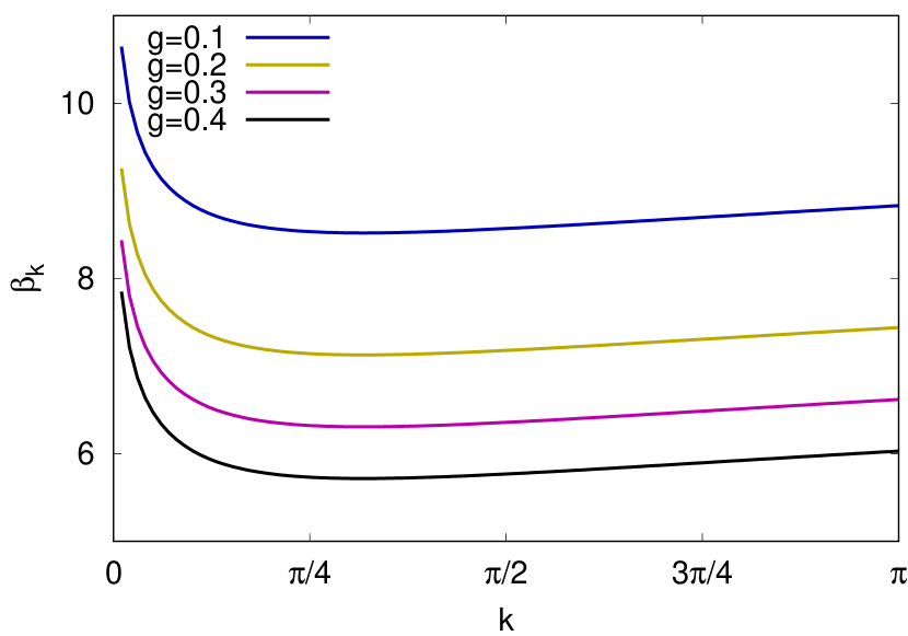
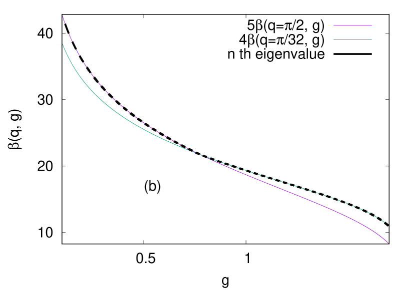
Figure 1: (a) One-particle spectrum $\beta_{C,k}=\beta_{S,k}=\beta_{k}$ of the entanglement Hamiltonian for various coupling strengths $g$ at zero temperature. (b) Crossing of different eigenvalues of the entanglement Hamiltonian. Here and in the following $\omega_{0}=M=v_{F}=1$.

We first find that the root of ${\langle\hat{p}^{2}_{S/C,q}\rangle}/{\langle\hat{q}^{2}_{S/C,q}\rangle}$ is $\alpha_{C/S,q}$. Then we realized, that the product of these (${\langle\hat{p}^{2}_{S/C,q}\rangle}{\langle\hat{q}^{2}_{C/S,q}\rangle}$) is related to the occupation numbers. With these findings all parameters can be determined as follows:

$$\alpha_{C/S,k} =\sqrt{\frac{\langle\hat{p}^{2}_{S/C,k}\rangle}{\langle\hat{q}^{2}_{S/C,k}\rangle}}\;,$$ (60)

$$\beta_{C/S,k} =\ln\left(1+\frac{1}{\sqrt{\langle\hat{p}^{2}_{S/C,k}\rangle\langle\hat{q}^{2}_{S/C,k}\rangle}-1/2}\right)\;.$$ (61)

These equations together with similar ones for the reduced density matrix of the phonons presented in Appendix B form the main result of this paper.

Generally, we have $\alpha_{C,k}\neq\alpha_{S,k}$, and $\beta_{S,k}\neq\beta_{C,k}$, but at zero temperature $\beta_{S,k}=\beta_{C,k}$. The bosonic $B_{s,q}$ and $B_{c,q}$ operators are related to the original bosonized $b_{q}$ operators and the ladder operators of the Harmonic oscillator through a Bogoliubov transformation.

From Eq. (59) it further follows that $\beta_{s,q}$, $\beta_{c,q}$ are the one-particle eigenvalues of the entanglement Hamiltonian $H_{\rm ent}=-\log\rho$, which is a bosonic free particle Hamiltonian. This one-particle spectrum of the entanglement Hamiltonian for various coupling strengths is shown in Fig. 1 (a). Please note that the full entanglement spectrum is not simply the set of the one-particle eigenvalues of the entanglement Hamiltonian. Even in our case of a free bosonic entanglement Hamiltonian, the spectrum of$H_{\rm ent}$ still includes all multiples of the one-particle eigenvalues (and all combination of different multiples).

Although the one-particle eigenvalues (as a function of the coupling strength) do not cross each other, there can hence still be level crossings in the full entanglement spectrum. An illustrative example is shown in Fig. 1 (b). If one arranges the entanglement eigenvalues by magnitude, the crossing simply implies a break in the derivative of the nth entanglement eigenvalue [but the eigenvalue itself remains a continuous function of the coupling, see Fig. 1 (b).]

In vladimir2020 it has been found by exact diagonalization of a Peierls-type Hamiltonian, that the entanglement spectrum is a nonanalytical function of the coupling strength, the $n$th entanglement eigenvalue is a continuous function of the coupling strength, but its derivative is not continuous. Our integrable model gives a simple explanation at least for some similar singularities. Due to the finite bandwidth of the Holstein Hamiltonian, singularities of a different origin may appear. Indeed not all singularities presented in vladimir2020 seems to be consistent with level crossing. On the other hand, the results of vladimir2020 result from exact diagonalization; and despite the usage of state-of-art methods, only a very small part of the entanglement spectrum can be explored with exact diagonalization. Hence, we do think that the crossing presented here exist also in finite bandwidth systems, but additional singularities may originate from th band-edge.

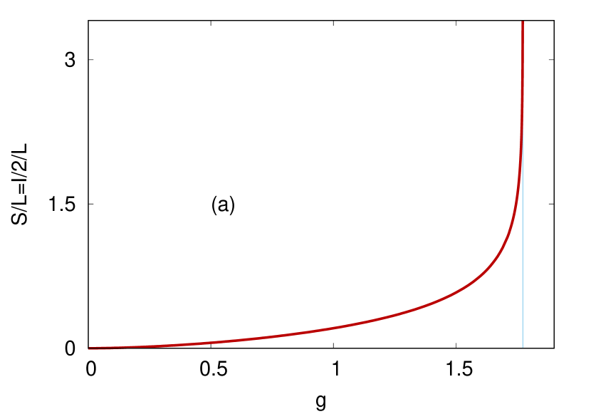
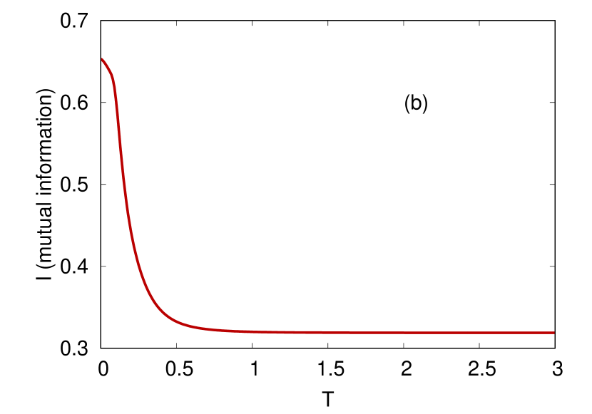
Figure 2: Upper panel: Entanglement entropy $S$ for the electronic subsystem (with a bipartition into electrons and phonons) as the function of the coupling strength $g$ for the ground state. Lower panel: Mutual information $I$ as the function of temperature at interaction $g=0.1$.

V Entanglement measures at zero and finite temperature

In this, section we present result for the entanglement entropy

$$S\equiv S_{e}=-{\rm Tr}\rho\log\rho$$ (62)

for the ground and thermally excited state with the reduced density operator $\rho$ for the electronic subsystem given by Eq. (55), and for the mutual information

$$I=S_{e}+S_{\rm ph}-S_{tot}\;,$$ (63)

where $S_{\rm ph}$ and $S_{tot}$ are in analogy to Eq. (62) the entanglement entropies of the phonon (see Appendix B) and total system, respectively. The results for the present model are shown in Fig. 2 (see Appendix A for calculational details). The entanglement entropy $S$ grows with the electron-phonon coupling strength $g$ and diverges at the Wentzel-Bardeen singularity. At zero temperature [panel (a)], the mutual information is $I=2S$ since for our bipartition $S_{e}=S_{\rm ph}$ and $S_{tot}=0$. However, at finite temperatures $T>0$ [panel (b)], neither of the latter two equations hold and there are deviations. Specifically, the mutual information decreases with increasing temperature, and after a local minimum around $T\approx 0.6$ reaches a plateau value for $T\to\infty$.

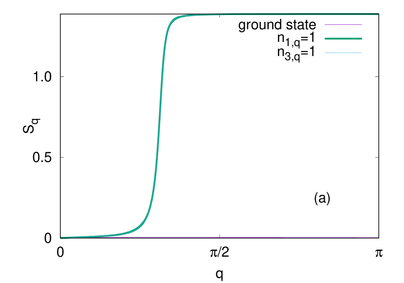
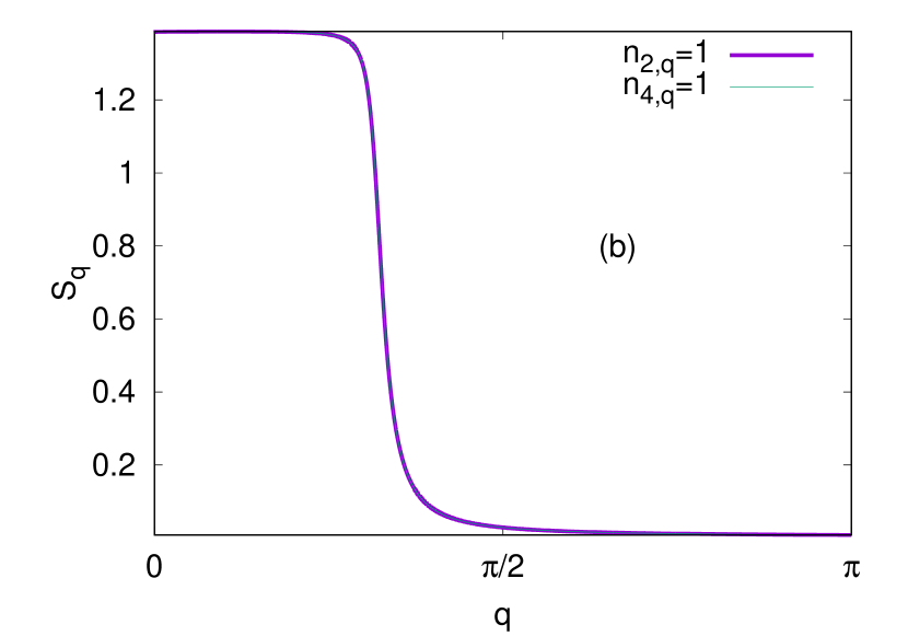
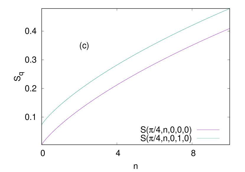
Figure 3: (a) Entanglement content of the mode with momentum $q$ in the ground state, and in the excited state with $n_{1,q}=1$ ($n_{3,q}=1$) and all other occupation numbers zero. Here and for all subpanels $g=0.1$. (b) Entanglement content of the mode with momentum $q$ in the excited states where $n_{2,q}=1$ ( $n_{4,q}=1$) and all other occupation numbers are zero. (c) Entanglement content of the excited state with $n_{1,\pi/4}\neq 0$ and all other occupation number zero as the function of the occupation number $n=n_{1,\pi/4}$ (purple line). The green line shows the entanglement content of the excited state where $n_{1,\pi/4}\neq 0$ and, in addition, $n_{3,\pi/4}=1$. The sum of the entanglement contents of the two states with only one non-zero occupation number (blue line) differs from the state where both are excited simultaneously (green line).

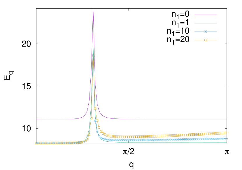
Figure 4: Logarithmic entanglement negativity content of modes with a given wave number at coupling $g=0.1$; $v_{F}=M=\omega_{0}=1$.

VI Entanglement content of excited states

In this section, we investigate the electron-phonon entanglement content of excited states $|\{n_{i,k}\}\rangle$. The entanglement entropy can be written as (see Appendix A)

$$S=\sum_{q>0}s(\langle\hat{p}^{2}_{C,q}\rangle\langle\hat{q}^{2}_{C,q}\rangle)+s(\langle\hat{p}^{2}_{S,q}\rangle\langle\hat{q}^{2}_{S,q}\rangle)$$ (64)

with $s(x)=(\sqrt{x}+1/2)\ln(\sqrt{x}+1/2)-(\sqrt{x}-1/2)\ln(\sqrt{x}-1/2)$. It is clear from Eq. (64), that the entanglement content of the different momenta is additive $S=\sum_{q}S_{q}$. This agrees with Ref. szecsenyi2018, and confirms Eq. (1), and further shows that a generalization to non-spatial bipartitions is possible. However, the entanglement content of the excitations $b^{\dagger}_{i,q}$ at the same momentum is not linearly additive for $i=1\dots 4$. If it was additive, the green and blue lines in Fig. 3 (c) would coincide. The entanglement is also not proportional to the occupation number as observed in Ref. pizorn2012, : clearly the red line in Fig. 3 (c) is not linear. The entanglement content of the 1st and 3rd and the 2nd and 4th kind of excitations are equal, see panels (a) and (b) of Fig. 3.

The entanglement negativity can be written as the following sum over the momentum

$${\cal E}=-2\sum_{q=0,\pm}^{q_{cutoff}}\ln\textnormal{min}(1,\sqrt{\Lambda_{C,q,\pm}})+\ln\textnormal{min}(1,\sqrt{\Lambda_{S,q,\pm}}),$$ (65)

the derivation and the $\Lambda_{C/S,k,\pm}$ values are given in Appendix C. In Fig. 4 the terms corresponding to a given momentum $k$ are shown for different occupation numbers $n_{1}$. Quite surprisingly, the contribution of a given mode to the entanglement negativity varies in a non-monotonic way with the occupation number. For small occupations the negativity become smaller then the ground state negativity, before starting to increase again for high occupation numbers. This is a rather different behavior than the entanglement entropy. The entanglement entropy always grows wit excitations, one can define a positive entanglement content for each one-particle excitation. As we have seen, the negativity can decrease with one-particle excitations. If one defines a ”negativity content of excitations”, this content could be positive or negative.

VII Conclusion and outlook

We have derived an analytical formula for the the entanglement entropy and the entanglement spectrum of a Luttinger liquid coupled to an Einstein phonon. The entanglement spectrum is $\sum_{q>0}\beta_{C,q}n_{C,q}+\sum_{q>0}\beta_{S,k}n_{S,q}$, where $n_{C,q}=0,\,1,\,2,\dots$ and $n_{S,q}=0,\,1,\,2,\dots$ are the occupation numbers and $\beta_{C/S,q}$ from Eq. (61) the eigenvalues of the bosonic modes of the entanglement Hamiltonian. The entanglement spectrum and thus the entanglement entropy is additive in momentum $q>0$. For each $q$ the Luttinger liquid coupled to Einstein phonons has four bosonic eigenmodes $\beta_{i,q}$, $i=1\ldots 4$, because $q$ and $-q$ couple into independent sine ($S$) and cosine ($C$) linear combinations dora2017 . For each of these in turn, electrons and phonons couple into two bosonic eigenmodes. In terms of the occupation of these four eigenmodes $\beta_{i,q}$ at fixed $q$, the entanglement entropy is not additive. In other words, while the momentum additivity conjectured in Eq. (1) holds in our model, there is no such additivity for the quasi-particle excitations at each momentum. As in exact diagonalization for a Peierls-type Hamiltonian vladimir2020 , we find that the entanglement spectrum is a nonanalytical function of the coupling strength, caused by a level crossing of the eigenvalues.

In our calculations, we did not include the electron spin. If included, there will be spin modes and charge modes, and only the charge modes couple to the phonon system. Another simple way of generalization is to include the Coulomb interaction between the electrons, but the main effect of these in a Luttinger liquid is the renormalization of the Fermi velocity.

Our results are predominately of fundamental, theoretical interest. However, for prospective applications let us mention that similar one-dimensional electron-phonon models describe the low energy behavior of carbon nanotubes suzuura2002 ; rosati2015 ; martino2003 ; benyamini2014 and the surface states of thin topological insulator wires egger2010 ; dorn2020 . There are also three-dimensional systems such as Li_0.9Mo₆O₁₇ giamarchi2012 where the electron system is quasi one-dimensional, and can be modeled as several parallel chain, each described by the Luttinger theory. For these systems, our results provide a first, general point of understanding, which need to be further detailed to actually describe these materials. Another non-trivial generalization for higher dimension is the inclusion the phonons to the coupled-wire description of topological systems meng2020 .

Appendix A Calculation of the entanglement entropy and the mutual information

The von Neumann entropy of the reduced density matrix is the entanglement entropy in the case of pure states (e.g. at zero temperature). It is also used in the definition of the mutual information in the case of general (for example thermal) states. The calculation of this quantity has been published in peschel2012 ; audenaert2002 ; roosz2020 , but to be self-contained we summarize it here in a nutshell.

The investigated subsystem contains $N$ bosonic modes with $\hat{q}_{1}\dots\hat{q}_{N}$ and $\hat{p}_{1}\dots\hat{p}_{N}$ canonical conjugated position-momentum operators with $[q_{i},p_{j}]=i\delta_{i,j}$. To calculate the entropy one first evaluates all pair-correlation functions $Q_{ij}=\langle\hat{q}_{i}\hat{q}_{j}\rangle$ and $P_{i,j}=\langle\hat{p}_{i}\hat{p}_{j}\rangle$ and $\text{Re}\langle\hat{q}_{1}\hat{p}_{l}\rangle$. Next, one forms the following correlation matrix of the correlation functions:

$$M=\left(\begin{array}[]{cccccc}\langle\hat{q}_{1}\hat{q}_{1}\rangle&\dots&\langle\hat{q}_{1}\hat{q}_{l}\rangle&\text{Re}\langle\hat{q}_{1}\hat{p}_{1}\rangle&\dots&\text{Re}\langle\hat{q}_{1}\hat{p}_{l}\rangle\\ \vdots&&\vdots&\vdots&&\vdots\\ \langle\hat{q}_{l}\hat{q}_{1}\rangle&\dots&\langle\hat{q}_{l}\hat{q}_{l}\rangle&\text{Re}\langle\hat{q}_{l}\hat{p}_{1}\rangle&\dots&\text{Re}\langle\hat{q}_{l}\hat{p}_{l}\rangle\\ \text{Re}\langle\hat{p}_{1}\hat{q}_{1}\rangle&\dots&\text{Re}\langle\hat{p}_{1}\hat{q}_{l}\rangle&\langle\hat{p}_{1}\hat{p}_{1}\rangle&\dots&\langle\hat{p}_{1}\hat{p}_{l}\rangle\\ \vdots&&\vdots&\vdots&&\vdots\\ \text{Re}\langle\hat{p}_{l}\hat{q}_{1}\rangle&\dots&\text{Re}\langle\hat{p}_{l}\hat{q}_{l}\rangle&\langle\hat{p}_{l}\hat{p}_{1}\rangle&\dots&\langle\hat{p}_{l}\hat{p}_{l}\rangle\end{array}\right).$$ (66)

Now one has to diagonalize the matrix using symplectic transformations and in this way obtain the symplectic spectrum $\Lambda_{1}\dots\Lambda_{N}$. Every eigenvalue of the $M$ matrix is twice degenerated, so $N$ numbers gives the symplectic spectrum of this $2N\times 2N$ matrix. Having the eigenvalues of the matrix in hand, one gets the entanglement entropy of the reduced density matrix as

$$S=\sum_{j=1}^{N}(\Lambda_{j}+1/2)\ln(\Lambda_{j}+1/2)-(\Lambda_{j}-1/2)\ln(\Lambda_{j}-1/2).$$ (67)

In our model, every coordinate-impulse correlation function is zero $\text{Re}\langle\hat{q}_{1}\hat{p}_{l}\rangle=0$. In this case, it can be shown that the square of the symplectic eigenvalues are the eigenvalues of the $PQ$ matrix, where $P$ is matrix containing all momentum-momentum functions (all of $\langle\hat{p}_{S,k}\hat{p}_{S,q}\rangle$ and $\langle\hat{p}_{C,k}\hat{p}_{C,q}\rangle$), and $Q$ is a matrix built up from the coordinate correlation functions in a similar manner.

When we consider the sinus-consinus modes defined in Eq. (11) and Eq. (13), the $QP$ matrix further become diagonal, and in the diagonal there are the $\langle\hat{p}_{S,k}^{2}\rangle$ and the $\langle\hat{p}_{C,k}^{2}\rangle$ values. This leads to the simple integral formula of Eq. (64).

Appendix B Density matrix of the phonons

With a similar reasoning as we used in the main text to derive the density matrix of the electrons, one can obtain the reduced density matrix of the phonons.

$$\rho =\Pi_{q>0}^{q_{\rm cutoff}}(1-e^{\beta^{Phonon}_{c,q}})e^{-\sum_{q}\beta^{Phonon}_{c,q}D^{\dagger}_{c,q}D_{c,q}}$$

$$\times\Pi_{q>0}^{q_{\rm cutoff}}(1-e^{\beta^{Phonon}_{s,q}})e^{-\sum_{q}\beta^{Phonon}_{s,q}D^{\dagger}_{s,q}D_{s,q}}$$

$$\times\rho_{q>q_{\rm cutoff}}^{\pi}\;.$$ (68)

Here $D^{\dagger}_{s,q}$, $D_{s,q}$, $D^{\dagger}_{c,q}$, $D_{c,q}$ are bosonic creation and annihilation operators, defined in the following way

$$D^{\dagger}_{S,q} =\sqrt{\frac{\gamma_{S,q}}{2}}(\hat{Q}_{S,q}+\frac{i}{\gamma_{S,q}}\hat{P}_{S,q})\;,$$ (69)

$$D_{S,q} =\sqrt{\frac{\gamma_{S,q}}{2}}(Q_{S,q}-\frac{i}{\gamma_{S,q}}\hat{P}_{S,q})\;,$$ (70)

$$D^{\dagger}_{C,q} =\sqrt{\frac{\gamma_{C,q}}{2}}(\hat{Q}_{C,q}+\frac{i}{\gamma_{C,q}}\hat{P}_{c,q})\;,$$ (71)

$$D_{C,q} =\sqrt{\frac{\gamma_{C,q}}{2}}(\hat{Q}_{C,q}-\frac{i}{\gamma_{C,q}}\hat{P}_{C,q})\;,$$ (72)

where the parameters $\gamma_{C,q}$, $\gamma_{S,q}$, $\beta_{C,q}$, $\beta_{S,q}$ are obtained in a similar way as in the case of the density matrix of the electrons, yielding

$$\gamma_{C/S,q} =\sqrt{\frac{\langle\hat{P}^{2}_{S/C,q}\rangle}{\langle\hat{Q}^{2}_{S/C,q}\rangle}}\;,$$ (73)

$$\beta^{Phonon}_{C/S,q} =\ln\left(1+\frac{1}{\sqrt{\langle\hat{P}^{2}_{S/C,q}\rangle\langle\hat{Q}^{2}_{S/C,q}\rangle}-1/2}\right)\;.$$ (74)

Here the expectation values of the squares of the bosonic operators are the following

$$\langle\hat{Q}^{2}_{C,q}\rangle=A^{2}_{k}\langle\hat{q}^{2}_{2,q}\rangle+B^{2}_{k}\langle\hat{q}^{2}_{1,q}\rangle\;,$$ (75)

$$\langle\hat{P}^{2}_{C,q}\rangle=A^{2}_{k}\langle\hat{p}^{2}_{2,q}\rangle+B^{2}_{k}\langle\hat{p}^{2}_{1,q}\rangle\;,$$ (76)

$$\langle\hat{Q}^{2}_{S,q}\rangle=A^{2}_{k}\frac{\omega^{2}_{4,q}}{\omega^{2}_{0}}\langle\hat{q}^{2}_{4,q}\rangle+B^{2}_{k}\frac{\omega^{2}_{3,q}}{\omega^{2}_{0}}\langle\hat{q}^{2}_{3,q}\rangle\;,$$ (77)

$$\langle\hat{P}^{2}_{S,q}\rangle=A^{2}_{k}\frac{\omega^{2}_{0}}{\omega^{2}_{4,q}}\langle\hat{p}^{2}_{4,q}\rangle+B^{2}_{k}\frac{\omega^{2}_{0}}{\omega^{2}_{3,q}}\langle\hat{p}^{2}_{3,q}\rangle\;.$$ (78)

Appendix C Calculation of the entanglement negativity

To calculate the entanglement negativity between the electrons and the phonons, one can consider the correlation matrix of the whole system, which is similar to $M$ in Eq. (66) but now contains all variables of the phonons and the bosonized fermions. Then one multiples all phonon momenta with $-1$. The thus transformed correlation matrix is the correlation matrix of the partial transpose of the density matrix.

One has to calculate the symplectic eigenvalues of the transformed matrix, let us denote these eigenvalues as $\lambda$. Then, the logarithmic negativity is calculated as

$${\cal E}=-\sum_{\lambda}\ln\min(1,\lambda)$$ (79)

In our problem the correlation matrix is block-diagonal, so one can find the symplectic eigenvalues block-by-block, and write the negativity as a sum over momentum.

$${\cal E}=-2\sum_{q=0,\pm}^{q_{\rm cutoff}}\ln\textnormal{min}(1,\sqrt{\Lambda_{C,q,\pm}})+\ln\textnormal{min}(1,\sqrt{\Lambda_{S,q,\pm}}),$$ (80)

where

$$\Lambda_{C/S,q,\pm}=\frac{1}{2}\left[a_{C/S,q}\pm\sqrt{a_{C/S,q}^{2}+4b_{C/S,q}-4c_{C/S,q}}\right]$$ (81)

with

$$a_{C/S,q} = \langle\hat{Q}_{C/S,q}\hat{Q}_{C/S,q}\rangle\langle\hat{P}_{C/S,q}\hat{P}_{C/S,q}\rangle+\langle\hat{q}_{C/S,q}\hat{q}_{C/S,q}\rangle\langle\hat{p}_{C/S,q}\hat{p}_{C/S,q}\rangle+2\langle\hat{P}_{C/S,q}\hat{p}_{C/S,q}\rangle\langle\hat{Q}_{C/S,q}\hat{q}_{C/S,q}\rangle,$$ (82)

$$b_{C/S,q} = \left(\langle\hat{Q}_{C/S,q}\hat{q}_{C/S,q}\rangle\langle\hat{P}_{C/S,q}\hat{P}_{C/S,q}\rangle-\langle\hat{q}_{C/S,q}\hat{q}_{C/S,q}\rangle\langle\hat{P}_{C/S,q}\hat{p}_{C/S,q}\rangle\right)$$ (83)

$$\times\left(\langle\hat{Q}_{C/S,q}\hat{q}_{C/S,q}\rangle\langle\hat{p}_{C/S,q}\hat{p}_{C/S,q}\rangle-\langle\hat{P}_{C/S,q}\hat{p}_{C/S,q}\rangle\langle\hat{Q}_{C/S,q}\hat{Q}_{C/S,q}\rangle\right),$$

$$c_{C/S,q} = \left(\langle\hat{Q}_{C/S,q}\hat{Q}_{C/S,q}\rangle\langle\hat{P}_{C/S,q}\hat{P}_{C/S,q}\rangle-\langle\hat{P}_{C/S,q}\hat{p}_{C/S,q}\rangle\langle\hat{Q}_{C/S,q}\hat{q}_{C/S,q}\rangle\right)$$ (84)

$$\times\left(\langle\hat{q}_{C/S,q}\hat{q}_{C/S,q}\rangle\langle\hat{p}_{C/S,q}\hat{p}_{C/S,q}\rangle-\langle\hat{P}_{C/S,q}\hat{p}_{C/S,q}\rangle\langle\hat{Q}_{C/S,q}\hat{q}_{C/S,q}\rangle\right).$$

References

- (1) E. Maxwell, Phys. Rev. 78, 477 (1950).
- (2) C. A. Reynolds, B. Serin, W. H. Wright, and L. B. Nesbitt, Phys. Rev. 78, 487 (1950).
- (3) W. D. Allen, R. H. Dawton, M. Bär, K. Mendelson, and J. L. Olsen, Nature (London) 166, 1071 (1950).
- (4) L. N. Cooper, Phys. Rev. 104, 1189 (1956).
- (5) J. Bardeen, L. N. Cooper, and J. R. Schrieffer, Phys. Rev. 106, 162 (1957).
- (6) J. Bardeen, L. N. Cooper, and J. R. Schrieffer, Phys. Rev. 108, 1175 (1957).
- (7) G. Roósz, C. Timm, Phys. Rev. B 104 (3), 035405 (2021)
- (8) R. E. Peierls, Quantum Theory of Solids, (Oxford University Press, Oxford, 1955), p. 108.
- (9) P. A. Lee, T. M. Rice, and P. W. Anderson, Phys. Rev. Lett. 31, 462 (1973).
- (10) B. Braunecker, G. I. Japaridze, J. Klinovaja, and D. Loss, Phys. Rev. B 82, 045127 (2010).
- (11) G. Grüner, Rev. Mod. Phys. 60, 1129 (1988).
- (12) A. Ványolos, B. Dóra, and A. Virosztek, Phys. Rev. B 73, 165127 (2006).
- (13) J. H. Miller, C. Ordóñez, and E. Prodan, Phys. Rev. Lett. 84, 1555 (2000).
- (14) A. B. Midgal, Sov. Phys. JETP 7, 996 (1958).
- (15) G. M. Éliashberg, Sov. Phys. JETP 11, 696 (1960).
- (16) A. S. Mishchenko, N. Nagaosa, and N. Prokof’ev, Phys. Rev. Lett. 113, 166402 (2014).
- (17) A. Mishchenko, N. Prokof’ev, A. Sakamoto, and B. Svistunov, Phys. Rev. B 62, 6317 (2000).
- (18) N. V. Prokof’ev and B. V. Svistunov, Phys. Rev. Lett. 81, 2514 (1998).
- (19) J. del Pino, F. A. Y. N. Schröder, A. W. Chin, J. Feist, and F. J. Garcia-Vidal, Phys. Rev. Lett. 121, 227401 (2018).
- (20) L. Amico, R. Fazio, A. Osterloh, and V. Vedral, Rev. Mod. Phys. 80, 517 (2008).
- (21) J. L. Sanz-Vicario, J. F. Pérez-Torres, and G. Moreno-Polo, Phys. Rev. A 96, 022503 (2017).
- (22) G. Wentzel, Phys. Rev. 83, 168 (1950).
- (23) J. Bardeen, Rev. Mod. Phys. 23, 3 (1951).
- (24) S. Engelsberg and B. B. Varga, Phys. Rev. 136, 14 (1964).
- (25) H. Suzuura and T. Ando, Phys. Rev. B 65, 235412 (2002).
- (26) R. Rosati, F. Dolcini, and F. Rossi, Phys. Rev. B 92, 235423 (2015).
- (27) A. De Martino and R. Egger, Phys. Rev. B 67, 235418 (2003).
- (28) A. Benyamini, A. Hamo, S. Viola Kusminskiy, F. von Oppen, and S. Ilani, Nature Phys. 10, 151 (2014).
- (29) M. I. Berganza, F. C. Alcaraz, G, Sierra J. Stat. Mech. 1201, P01016 (2012)
- (30) D. Loss and T. Martin, Phys. Rev. B 50, 16 (1994).
- (31) K. Audenaert, J. Eisert, M. B. Plenio, and R. F. Werner, Phys. Rev. A 66, 042327 (2002).
- (32) V. Eisler and Z. Zimborás, New J. Phys. 16, 123020 (2014).
- (33) J. von Delft and H. Schoeller, Annalen Phys. 7, 225 (1998).
- (34) F. Bloch, Z. Phys. 52, 555 (1929).
- (35) F. Giustino, Rev. Mod. Phys. 89, 015003 (2017).
- (36) I. Peschel, Braz. J. Phys. 42, 267 (2012).
- (37) B. Dóra, I. Lovas, and F. Pollmann, Phys. Rev. B 96, 085109 (2017).
- (38) A. Weisse, H. Fehske, G. Wellein, and A. R. Bishop, Phys. Rev. B 62, R747 (2000).
- (39) L.-C. Ku, S. A. Trugman, and J. Bonˇca, Phys. Rev. B 65, 174306 (2002)
- (40) Y. Toyozawa, Prog. Theor. Phys. 26, 29 (1961)
- (41) A. H. Romero, D. W. Brown, and K. Lindenberg, J. Chem. Phys. 109, 6540 (1998)
- (42) O. S. Barisic, Phys. Rev. B 65, 144301 (2002)
- (43) T. A. Costi, Ross H. McKenzie Phys. Rev. A 68, 034301 (2003)
- (44) V. M. Stojanovic, M. Vanevic Phys. Rev. B 78, 214301 (2008)
- (45) V. M. Stojanovic Phys. Rev. B 101, 134301 (2020)
- (46) Yang Zhao, Paolo Zanardi, and Guanhua Chen Phys. Rev. B 70, 195113 (2004)
- (47) R. Egger, A. Zazunov, and A. Levy Yeyati Phys. Rev. Lett. 105, 136403 (2010)
- (48) K. Dorn, A. De Martino, and R. Egger, Phase diagram and phonon-induced backscattering in topological insulator nanowires, Phys. Rev. B 101, 045402 (2020).
- (49) P. Chudzinski, T. N. Jarlborg, T. Giamarchi, Phys. Rev. B. 86, 075147 (2012)
- (50) T. Meng The European Physical Journal Special Topics 229 (4), 527-543 (2020)
- (51) O.A. Castro-Alvaredo, C. De Fazio, B. Doyon, I.M. Szécsényi PRL 121 (17), 170602 (2018)
- (52) O.A. Castro-Alvaredo, C. De Fazio, B. Doyon, I.M. Szécsényi Journal of Mathematical Physics 60 (8), 082301 (2019)
- (53) O.A. Castro-Alvaredo, C. De Fazio, B. Doyon, I.M. Szécsényi Journal of High Energy Physics 2019 (11), 1-47 (2019)
- (54) J. Mölter, T. Barthe, U. Schollwöck, V. Alba, J. Stat. Mech. 2014 (10), P10029 (2014)
- (55) I. Pizorn Universality in entanglement of quasiparticle excitations arXiv:1202.3336 (2012)
- (56) M. Storms, R. R. P. Singh Phys. Rev. E 89, 012125 (2014)
- (57) R. Berkovits Phys. Rev B 87, 075141 (2013)
- (58) V. Alba, M. Fagotti, P. Calabrese J. Stat. Mech 2009(10), P10020 (2009)
- (59) F. F. Assaad and T. C. Lang Phys. Rev. B 76, 035116 (2007)
- (60) C. Faugeras, M. Amado, P. Kossacki, M. Orlita, M. Sprinkle, C. Berger, W.A. de Heer, M. Potemski Phys. Rev. Lett. 103, 186803, (2009)
- (61) P. Postorino, A. Congeduti, P. Dore, A. Sacchetti, F. Gorelli, L. Ulivi, A. Kumar, and D. D. Sarma Phys. Rev. Lett. 91, 175501 (2003)