An Energy and Carbon Footprint Analysis of Distributed and Federated Learning

Abstract

Classical and centralized Artificial Intelligence (AI) methods require moving data from producers (sensors, machines) to energy hungry data centers, raising environmental concerns due to computational and communication resource demands, while violating privacy. Emerging alternatives to mitigate such high energy costs propose to efficiently distribute, or federate, the learning tasks across devices, which are typically low-power. This paper proposes a novel framework for the analysis of energy and carbon footprints in distributed and federated learning (FL). The proposed framework quantifies both the energy footprints and the carbon equivalent emissions for vanilla FL methods and consensus-based fully decentralized approaches. We discuss optimal bounds and operational points that support green FL designs and underpin their sustainability assessment. Two case studies from emerging 5G industry verticals are analyzed: these quantify the environmental footprints of continual and reinforcement learning setups, where the training process is repeated periodically for continuous improvements. For all cases, sustainability of distributed learning relies on the fulfillment of specific requirements on communication efficiency and learner population size. Energy and test accuracy should be also traded off considering the model and the data footprints for the targeted industrial applications.

I Introduction

Training deep Machine Learning (ML) models at the network edge has reached notable gains in terms of accuracy across many tasks, applications and scenarios. However, such improvements have been acquired at the cost of large computational and communication resources, as well as significant energy footprints which are currently overlooked. Vanilla ML requires all training procedures to be conducted inside data centers [1] that collect data from producers, such as sensors, machines and personal devices. Centralized based learning requires high energy costs for networking and data maintenance, while introduces privacy issues as well. In addition, many mission critical ML tasks require data centers to learn continuously [2] to track changes in dataset distributions. Data centers are thus becoming more and more energy-hungry and responsible of significant CO2 (carbon) emissions. These amount to about $15$% of the equivalent global Green House Gas (GHG) emissions of the entire Information and Communication Technology (ICT) ecosystem [3], estimated as $0.5\div 1$ GtCO2e (gigatonnes of CO2 equivalent emissions) in 2020. Electricity consumed by global data centers is also estimated to be between $1.1$% and $1.5$% of the total worldwide electricity use.

Emerging alternatives to centralized big-data analytics enable decisions to be made at much more granular levels [4]. The Federated Learning (FL) approach [5] is a recently proposed distributed AI paradigm [6] in line with this trend. Under FL, the ML model parameters, e.g. the weights and biases $\mathbf{W}$ of Deep Neural Networks (DNN), are collectively optimized across several resource-constrained edge/fog devices, that act as both data producers and local learners. FL distributes the computing tasks across many devices characterized by low-power consumption profiles, compared with data centers, and each device has access to small datasets [2] only. With a judicious system design taking into account both accuracy and energy, FL is expected to bring significant reduction in terms of energy footprints, obviating the need for a large centralized infrastructure for cooling or power delivery.

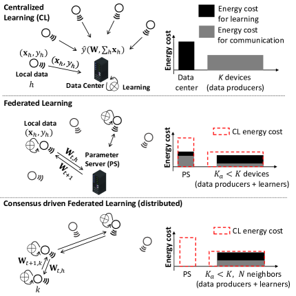
Figure 1: From top to bottom: Centralized Learning (CL), Federated Learning (FL) coordinated by the Parameter Server (PS), namely Federated Averaging (FA), and Consensus-driven Federated Learning, enabling fully decentralized implementations (i.e., without PS).

I-A Federated, consensus-driven and centralized learning: related works

As shown in Fig. 1, vanilla FL algorithms, such as Federated Averaging (FA) [4], allow devices to learn a local model under the orchestration of a Parameter Server (PS). Devices might be either co-located in the same geographic area or distributed in different zones. Typically, the PS aggregates the received local models to obtain a global model that is fed back to the devices. The PS functions are substantially less energy-hungry compared to centralized learning (CL) and can be implemented at the network edge. Different FL implementations have emerged in the past few years [7] targeting several scenarios [2, 8]. The optimization of the population of learners is critical in FL and is typically explored when power and bandwidth of devices are limited [9]. Delay and energy tradeoffs between learning and communication are considered in [10], while the problem of transmission scheduling in small-scale fading is analyzed in [11]. Quantization and compression of model parameters, or gradients, is useful to minimize bandwidth usage and to avoid straggler effects [12, 13, 14]. For a comprehensive survey on FL please refer to [4].

The above mentioned designs leverage on a server-client architecture [7] where the PS represents a single-point of failure and penalizes scalability. In analogy with distributed ledger, consensus-driven learning replaces the PS functions as it lets the local model parameters be consensually shared and synchronized across multiple devices via device-to-device (D2D) or sidelink communications [2]. Such fully decentralized solution relies solely on in-network processing and a consensus-based federation model, i.e., often based on distributed weighted averaging [15]-[18].

Regardless of whether the network architecture is server-client or decentralized via consensus methods, distributed learning requires many communication rounds for convergence that often consist of UpLink (UL) and DownLink (DL) communications through a Wireless Wide Area access and core Network (WWAN). Large energy bills might be therefore observed for communication [10]. The choice between distributed and centralized learning targeting sustainable, energy-aware designs is thus expected to be driven by communication vs computing cost balancing.

I-B Contributions

The paper develops a novel framework for the analysis of energy and carbon footprints in distributed ML, including, for the first time, comparisons and tradeoff considerations about vanilla, consensus-driven FL and centralized learning on the data center. Despite initial attempts to assess FL resource efficiency [8], optimize delay/energy [10, 11] and carbon footprints [3, 20], quantifying the optimal operating points towards green or sustainable setups is yet unexplored. To fill this void, the paper dives into the implementations of selected distributed learning tools, and discusses optimized designs and operational conditions with respect to energy-efficiency and low carbon emissions. A general framework is first developed for energy and carbon footprint assessment: differently from [3, 10], it considers all the system parameters and components of the learning process, including the PS, required in vanilla FL, as well as the distributed model averaging, required in decentralized setups. Next, sustainable regions in the parameter space are identified to steer the choice between centralized and distributed training in practical setups: the regions highlight bounds, or necessary conditions on communication, computing efficiencies, data and model size that make FL more promising than CL with respect to its carbon footprint. Unlike classical FL platforms [4, 10] defined on top of edge devices with large computing power [8], the paper focuses on learning tasks suitable for low-power embedded wireless devices (e.g., robots, vehicles, drones) typically adopted in Industrial Internet of Things (IIoT) applications [7]. These setups are characterized by devices/learners retaining small training datasets, while running medium/small-sized ML models due to their constrained internal memory. Devices are also equipped with low-power radio interfaces supporting deep sleep modes, cellular (e.g., 5G and NB-IoT), as well as direct mode, or sidelink, communication interfaces.

The proposed co-design of learning and communication is validated using real world data and a test-bed platform characterized by low-power devices implementing real-time distributed model training on top of the Message Queuing Telemetry Transport (MQTT) protocol. The real-time test-bed is used to measure the training time for different learning policies, while a what-if analysis quantifies the estimated energy and carbon footprints considering the impact of various communication settings, as well as the influence of the learner population size.

I-C Paper structure and organization

The paper is organized as follows. Section II describes the framework for energy consumption evaluation of different distributed learning strategies. Energy modelling is carried out separately for centralized learning (Sect.II-A), vanilla FA (Sect. II-B), including the novel policy FA-D that keeps inactive learners in deep-sleep, and decentralized consensus-driven FA (Sect. II-C). Necessary adaptations of the proposed energy models to continual and Reinforcement Learning (RL) paradigms [21] are also discussed in Sect. II-D.

Sect. III considers the carbon footprints (Sect. III-A) and the sustainable regions (Sect. III-B) that provide necessary requirements to steer the choice between centralized and distributed learning paradigms. Requirements are verified first in Sect. IV using the MNIST [22] and the CIFAR10 [23] datasets (Sect. IV-A) separately and through comparative analysis (Sect. IV-B). Next, practical design problems are explored in Sect. V targeting two industry relevant use cases. In particular, the FL network implementation is based on the MQTT protocol (Sect. V-A) while 4 communication efficiency profiles are considered (Sect. V-B). Both continual (Sect. V-C) and RL (Sect. V-D) scenarios are analyzed where the training process must be periodically repeated using new input data that change frequently to follow either a time-varying industrial process or the same model under training. These tools are critical in 5G industry verticals, i.e., Industry 4.0 (I4.0) applications, and could raise significant energy concerns unless specific actions are taken. Finally, conclusion are summarized in Sect. VI.

II Energy footprint modeling framework

The proposed framework provides insights into how the different components of the CL (i.e., the datacenter) and FL architectures (i.e. the local learners, the core network and the PS), contribute to the energy bill and to the carbon emissions in terms of system accuracy and number of rounds. The learning system consists of $K$ devices and one data center ($k=0$). Each device $k>0$ has a dataset $\mathcal{E}_{k}$ of examples $(\mathbf{x}_{h},y_{h})$ that are typically collected independently. In supervised learning, examples $\mathbf{x}_{h}$ are labelled as $y_{h}$ for training. Unsupervised setups, i.e., RL, are discussed in Sect. II-D. For all cases, the objective of the learning system is to train a DNN model $\hat{y}(\mathbf{W};\mathbf{x})$ that transforms the input data $\mathbf{x}$ into the desired $C$ outputs $\hat{y}\in\left\{y_{c}\right\}_{c=1}^{C}$, i.e., the output classes. Model parameters are here specified by the matrix $\mathbf{W}$ [4]. The training system uses the examples in $\mathcal{E}=\bigcup_{k=1}^{K}\mathcal{E}_{k}$ to minimize a loss function $L$ of the form

$$L(\mathcal{E}|\mathbf{W})=\sum_{k=1}^{K}L_{k}(\mathcal{E}_{k}|\mathbf{W}).$$ (1)

In what follows, unless stated otherwise, we use the cross-entropy loss function [4], namely $L_{k}=-\sum_{h}y_{h}\log\left[\hat{y}(\mathbf{W};\mathbf{x}_{h})\right]$. Minimization of (1) is typically iterative and gradient-based [5]: it runs over a pre-defined number ($n$) of learning rounds that depend on a specified target loss threshold, namely $L(\mathcal{E}|\mathbf{W})\leq\overline{\xi}$, i.e., corresponding to a required accuracy. For example, using Stochastic Gradient Descent (SGD)

$$\mathbf{W}_{t+1}\leftarrow\mathbf{W}_{t}-\mu_{s}\times\nabla L_{k}(\mathcal{E}_{k}|\mathbf{W}_{t}),$$ (2)

examples $\mathcal{E}_{k}$ are drawn randomly from the full training set $\mathcal{E}$, while $\mu_{s}$ is the step-size and $\nabla L_{k}(\mathcal{E}_{k}|\mathbf{W}_{t})=\nabla_{\mathbf{W}_{t}}\left[L(\mathcal{E}_{k}|\mathbf{W}_{t})\right]$ is the gradient of the loss function (1) over the assigned batches of data $\mathcal{E}_{k}$ given the model $\mathbf{W}_{t}$.

The energy footprint of device $k$, namely the total amount of energy consumed by the learning process, is broken down into computing and communication components. Considering one learning round, all the energy costs are modelled as a function of the computing energy $E_{k}^{(\mathrm{C})}$ required by the optimizer (2) and the energy $E_{k,h}^{(\mathrm{T})}$ per correctly received/transmitted bit over the wireless link ($k,h$). The training data or the DNN model parameters are quantized before transmission into $b(\mathcal{E}_{k})$ and $b(\mathbf{W})$ bits, respectively. The quantization scheme assigns a fixed number of bits (here 32 bits) to each parameter of the DNN model. Compression techniques such as model pruning, sparsification [24], parameter selection and/or differential transmission schemes [12, 25] are extremely helpful to scale down the footprint $b(\mathbf{W})$ in large DNNs. However, due to the great variety of compression techniques, we have considered here only a simple quantization scheme. The modifications to include a particular technique can be trivially detailed using the specific data $b(\mathcal{E}_{k})$ and model size $b(\mathbf{W})$ as the result of the compression processes.

We define the energy cost for UL communication with the data center (or the PS), co-located with the Base Station (BS), as $E_{k,0}^{(\mathrm{T})}$. Similarly, $E_{0,k}^{(\mathrm{T})}$ refers to DL communication, i.e., from the PS, or the BS, to the k-th device. Communication costs incorporate both transmission and decoding operations [26]. In contrast to digital implementations, analog FL designs [9, 17] get over the restrictions of time scheduled access: rather than spending energy $E_{k,h}^{(\mathrm{T})}$ for sending bits over orthogonal links, they exploit the superposition property of wireless transmissions for analog aggregation [27], scaling down the number of channel uses, and the communication cost. Although not considered in this paper, comparing analog and digital FL in the light of energy footprints is an open problem of wide interest. The energy $E_{k}^{(\mathrm{C})}$ for computing includes the cost of the learning round, namely the local gradient-based optimizer and the data storage costs. All costs are quantified on average: notice that routing through the radio access and the core network can vary but might be assumed as stationary apart from failures or replacements.

II-A Centralized Learning

Under CL, the model training is carried out inside the data center $k=0$, assumed co-located with the BS, and exploits the processing power provided by racks of CPU (Central Processing Units), GPU (Graphic Processing Units) and other specialized AI accelerators such as NPU (Neural Processing Units) and TPU (Tensor Processing Units). Therefore, the energy cost per round $E_{0}^{(\mathrm{C})}=P_{0}\cdot T_{0}\cdot B$ depends on the power consumption $P_{0}$ [20] of the aforementioned hardware units, the time span $T_{0}$ required for processing an individual batch of data, i.e. minimizing the loss $L(\cdot|\mathbf{W})$, and the number $B$ of batches per round [10]. Data are collected independently by the devices while we neglect here the cost of initial dataset loading since it is a one-step process only. For $n$ rounds, chosen to satisfy a target loss $\overline{\xi}$, the total energy $E_{\mathrm{CL}}$ in Joule [J] consists of computing $E_{\mathrm{CL}}^{(\mathrm{L})}$ and communication $E_{\mathrm{CL}}^{(\mathrm{C})}$ costs:

$$E_{\mathrm{CL}}(n)=\underset{E_{\mathrm{CL}}^{(\mathrm{L})}}{\underbrace{\gamma\cdot n\cdot E_{0}^{(\mathrm{C})}}}+\underset{E_{\mathrm{CL}}^{(\mathrm{C})}}{\underbrace{\alpha\cdot\sum_{k=1}^{K}b(\mathcal{E}_{k})\cdot E_{k,0}^{(\mathrm{T})}}.}$$ (3)

The energy cost for computing inside the data center scales as $E_{\mathrm{CL}}^{(\mathrm{L})}(n)=\gamma\cdot n\cdot E_{0}^{(\mathrm{C})}$ with $\mathrm{\gamma}>1$ being the Power Usage Effectiveness (PUE) of the data center [31, 32]. The PUE accounts for the additional power consumed for data storage, power delivery and cooling: $\gamma$ values are in the range $1.1\div 1.8$ [32, 44]. The energy consumed for communication of raw data is $E_{\mathrm{CL}}^{(\mathrm{C})}=\alpha\sum_{k=1}^{K}b(\mathcal{E}_{k})\cdot E_{k,0}^{(\mathrm{T})}$ and quantifies the energy for moving $b(\mathcal{E}_{k})$ bits of the $k$-th local training dataset $\mathcal{E}_{k}$ for $\alpha$ times and for all the $K$ devices. Parameter $\alpha$ counts the number of times a new training dataset is uploaded by the devices while learning is in progress. For example, in one-time learning processes, the full training dataset is available by devices before the training starts: therefore, it is $\alpha=1$. On the other hand, in continual learning applications, devices produce new training data continuously [2, 21]: data thus needs to be moved while learning is in progress, therefore it is $1<\alpha\leq n$.

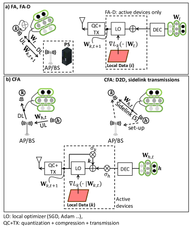
Figure 2: Distributed learning algorithms: a) Federated Averaging (FA, FA-D), b) CFA with sidelink communications.

II-B Federated learning with server (FA) and deep-sleep (FA-D)

Unlike CL, FL distributes the learning process across a selected, typically time-varying [4], subset $\mathcal{N}_{t}$ of $K_{a}<K$ active devices as shown in Fig. 1(a). At each round $t$, the local dataset $\mathcal{E}_{k}$ is used to train the local model $\mathbf{W}_{k,t}$ using a gradient-based Local Optimizer (LO) and a global model instance ($\mathbf{W}_{t}$), obtained from the server (PS). The goal is to minimize the local loss $L_{k}$ as

$$\mathbf{W}_{k,t}=\underset{\mathbf{W}}{\mathrm{arg}\mathrm{min}}\thinspace L_{k}(\cdot|\mathbf{W})+\upsilon\left\|\mathbf{W}-\mathbf{W}_{t}\right\|^{2},$$ (4)

where $\upsilon\left\|\mathbf{W}-\mathbf{W}_{t}\right\|^{2}$ is the proximal term [11, 28] often used when data is non-identically distributed (non-IID). The local model $\mathbf{W}_{k,t}$ is then forwarded to the PS [4] over the UL. The PS is co-located with the BS and is in charge of updating the global model $\mathbf{W}_{t+1}$ for the following round $t+1$ through the aggregation of the $K_{a}$ received models [5]:

$$\mathbf{W}_{t+1}\leftarrow\sum_{k\in\mathcal{N}_{t}}\sigma_{k}\cdot\mathbf{W}_{k,t},$$ (5)

with $\sigma_{k}=\tfrac{Q_{k}}{Q}$ being the ratio between the number of local examples $Q_{k}$ and global $Q=\sum_{k\in\mathcal{N}_{t}}Q_{k}$ ones, respectively. Notice that for IID data distributions, it is $\sigma_{k}=\tfrac{1}{K_{a}}$ [6]. The new model $\mathbf{W}_{t+1}$ is finally sent back to the devices over the DL.

Federated Averaging (FA). In vanilla FL methods, such as FA, the PS chooses $K_{a}<K$ active devices on each round to communicate their local model. During this process, the remaining $K-K_{a}$ devices are powered on [5, 6] as they run the LO (4) and decode the updated global model $\mathbf{W}_{t}$ obtained from the PS. For $n$ rounds, the total end-to-end energy can be written as

$$E_{\mathrm{FA}}(n)=E_{\mathrm{FA}}^{(\mathrm{L})}(n)+E_{\mathrm{FA}}^{(\mathrm{C})}(n),$$ (6)

namely, the superposition of the computing $E_{\mathrm{FA}}^{(\mathrm{L})}(n)$ and the communication $E_{\mathrm{FA}}^{(\mathrm{C})}(n)$ costs, considering both the devices and the PS consumption. In particular:

$$\begin{array}[]{c}E_{\mathrm{FA}}^{(\mathrm{L})}(n)=\gamma\cdot n\cdot\beta\cdot E_{0}^{(\mathrm{C})}\,+n\cdot\sum_{k=1}^{K}E_{k}^{(\mathrm{C})},\\ E_{\mathrm{FA}}^{(\mathrm{C})}(n)=b(\mathbf{W})\left[n\cdot\sum_{k=1}^{K}\gamma\cdot E_{0,k}^{(\mathrm{T})}+\sum_{t=1}^{n}\sum_{k\in\mathcal{N}_{t}}E_{k,0}^{(\mathrm{T})}\right].\end{array}\begin{aligned} \end{aligned}$$ (7)

The energy cost for computing $E_{\mathrm{FA}}^{(\mathrm{L})}(n)$ in (7) is due to the PS energy $\gamma\cdot n\cdot\beta\cdot E_{0}^{(\mathrm{C})}$ needed for model averaging and the LO, $n\cdot\sum_{k=1}^{K}E_{k}^{(\mathrm{C})}$ that is implemented by all the $K$ devices [10]. The energy for model averaging $\beta\cdot E_{0}^{(\mathrm{C})}$ is considerably smaller than the gradient-based optimization term $E_{0}^{(\mathrm{C})}$ on the data center, therefore it is $\beta\ll 1$. In IoT setups, the devices are also usually equipped with embedded low-consumption CPUs, SoCs (System on Chips) or $\mu$CU (microcontrollers): thus, it is reasonable to assume $E_{k}^{(\mathrm{C})}<E_{0}^{(\mathrm{C})}$. The communication energy $E_{\mathrm{FA}}^{(\mathrm{C})}(n)$ in (7) models the cost of the global model transmission over the DL, i.e., $n\cdot b(\mathbf{W})\sum_{k=1}^{K}\gamma\cdot E_{0,k}^{(\mathrm{T})}$, and the UL communication from selected $K_{a}$ active devices, i.e., $b(\mathbf{W})\sum_{t=1}^{n}\sum_{k\in\mathcal{N}_{t}}E_{k,0}^{(\mathrm{T})}$ in the set $\mathcal{N}_{t}$: as depicted in Fig. 2(a), it is assumed that the PS is co-located with the BS. The model size $b(\mathbf{W})$ quantifies the size in bits of model parameters to be exchanged. As analyzed in the Sect. III, both model $b(\mathbf{W})$ and local data size $b(\mathcal{E}_{k})$ are critical for sustainable designs. Notice that, as opposed to data, $b(\mathbf{W})$ is roughly the same for each device, although small changes might be observed when using lossy compression, sparsification or parameter selection methods [12, 24, 25].

Federated Averaging with deep-sleep (FA-D). An alternative to FA, referred to as FA-D, lets the inactive $K-K_{a}$ devices to turn off their computing hardware and communication interface, and set into a deep-sleep mode, when not needed by the PS. Deep sleep mode should be paired with efficient hardware able to power up and down in fractions of milliseconds: this is also a key component of 5G [26] and supported by popular interfaces, such as NB-IoT [47]. In contrast to vanilla FA, FA-D limits the consumption to the $K_{a}$ active devices, while these might change from round to round on a duty-cycle basis. As verified in the following, FA-D brings significant per-round energy benefits, in exchange for larger number of rounds $n_{\mathrm{FA-D}}>n_{\mathrm{FA}}$, for the same target accuracy $\overline{\xi}$. Considering the duty cycling process, the energy footprint of FA-D becomes

$$E_{\mathrm{FA-D}}(n)=E_{\mathrm{FA-D}}^{(\mathrm{L})}(n)+E_{\mathrm{FA-D}}^{(\mathrm{C})}(n),$$ (8)

now with

$$\begin{array}[]{c}E_{\mathrm{FA-D}}^{(\mathrm{L})}(n)=\gamma\cdot n\cdot\beta\cdot E_{0}^{(\mathrm{C})}\,+\sum_{t=1}^{n}\left[\sum_{k\in\mathcal{N}_{t}}E_{k}^{(\mathrm{C})}+\sum_{k\notin\mathcal{N}_{t}}E_{k,\mathrm{sleep}}^{(\mathrm{C})}\right],\\ E_{\mathrm{FA-D}}^{(\mathrm{C})}(n)=b(\mathbf{W})\cdot\sum_{t=1}^{n}\sum_{k\in\mathcal{N}_{t}}\left[\gamma\cdot E_{0,k}^{(\mathrm{T})}+E_{k,0}^{(\mathrm{T})}\right].\end{array}\begin{aligned} \end{aligned}$$ (9)

Notice that the LO cost is now constrained to the active devices, $\sum_{t=1}^{n}\sum_{k\in\mathcal{N}_{t}}E_{k}^{(\mathrm{C})}$ as with global model communication, $b(\mathbf{W})\cdot\sum_{t=1}^{n}\sum_{k\in\mathcal{N}_{t}}\gamma\cdot E_{0,k}^{(\mathrm{T})}$. Finally, $E_{k,\mathrm{sleep}}^{(\mathrm{C})}$ accounts for the energy consumption of inactive devices in deep-sleep mode (if not negligible w.r.t. $E_{k}^{(\mathrm{C})}$ ).

II-C Consensus-driven Federated Averaging (CFA)

Decentralized FL techniques [16, 17, 18] let the devices mutually exchange their local models, possibly over peer-to-peer networks. Unlike with FA, the PS is not needed as it is replaced by a consensus mechanism. In particular, we propose a consensus-driven FA approach (CFA) where the federated nodes exchange the local ML model parameters and update them sequentially by distributed averaging. As shown in Fig. 2(b), devices mutually exchange their local model parameters $\mathbf{W}_{k,t}$ with an assigned number $N$ of neighbors [12, 13, 17]. Distributed weighted averaging [16, 18] is used to combine the received models.

Let $\mathcal{N}_{k,t}$ be the set that contains the $N$ chosen neighbors of node $k$ at round $t$: on every new round ($t>0$), the device updates the local model $\mathbf{W}_{k,t}$ using the parameters $\mathbf{W}_{h,t}$ obtained from the neighbor device(s) as

$$\mathbf{W}_{k,t+1}\leftarrow\mathbf{W}_{k,t}+\sum_{h\in\mathcal{N}_{k,t}}\sigma_{h,k}\cdot(\mathbf{W}_{h,t}-\mathbf{W}_{k,t}),$$ (10)

where the weights $\sigma_{h,k}$ are chosen to guarantee a stable solution as

$$\sigma_{h,k}=\frac{Q_{h}}{\sum_{h\in\mathcal{N}_{k,t}}Q_{h}},$$ (11)

and for IID data, it is $\sigma_{h,k}=\tfrac{1}{N}$, $\forall h,k$. Distributed weighted averaging (10) is followed by LO (4) on $\mathcal{E}_{k}$ that can also include proximal regularization [28]. For $K_{a}<K$ active devices in the set $\mathcal{N}_{t}$ and $n$ rounds, the energy footprint is again broken down into learning and communication costs as

$$E_{\mathrm{CFA}}(n)=E_{\mathrm{CFA}}^{(\mathrm{L})}(n)+E_{\mathrm{CFA}}^{(\mathrm{C})}(n),$$ (12)

with

$$\begin{array}[]{c}E_{\mathrm{CFA}}^{(\mathrm{L})}(n)=\sum_{t=1}^{n}\left[\sum_{k\in\mathcal{N}_{t}}E_{k}^{(\mathrm{C})}+\sum_{k\notin\mathcal{N}_{t}}E_{k,\mathrm{sleep}}^{(\mathrm{C})}\right],\\ E_{\mathrm{CFA}}^{(\mathrm{C})}(n)=\sum_{t=1}^{n}\sum_{k\in\mathcal{N}_{t}}\sum_{h\in\mathcal{N}_{k,t}}b(\mathbf{W}_{k,t})\cdot E_{k,h}^{(\mathrm{T})}.\end{array}\begin{aligned} \end{aligned}$$ (13)

The sum $\sum_{h\in\mathcal{N}_{k,t}}b(\mathbf{W}_{k,t})\cdot E_{k,h}^{(\mathrm{T})}$ now models the total energy spent by the device $k$ to diffuse the local model parameters to selected neighbors $h$ in the set $\mathcal{N}_{t}$ at round $t$. Since the PS is not used, CFA is particularly promising in reducing the energy footprint.

CFA requires sending data over peer-to-peer links ($k,h$): in WWAN, each link is implemented by UL transmission from the source $k$ to the core network access point (i.e., router or BS), followed by a DL communication from the router(s) to the destination device $h$, therefore

$$E_{k,h}^{(\mathrm{T})}=E_{k,0}^{(\mathrm{T})}+\gamma\cdot E_{0,h}^{(\mathrm{T})},$$ (14)

where $\gamma$ is the PUE of the BS or router hardware (if any). Alternatively, CFA can leverage direct, or sidelink, transmissions [29]. Sidelink (SL) features were introduced by 3GPP (PC5 interface) in release $12$ and $13$, namely the proximity service (ProSe). They support direct (D2D) communications with minor involvement of the BS, or eNB [19, 41]. Since the signal relay through the BS is not needed, excluding an initial link setup for resource allocation, sidelink communications are expected to make a significant step towards green and sustainable networks, serving as enabling technology for an efficient implementation of CFA. Both communication architectures will be addressed next.

II-D Continual and reinforcement learning paradigms

The energy framework previously discussed is suitable for modelling the environmental footprints of conventional supervised, or one-time, ML problems. On the other hand, novel learning paradigms are emerging in industrial IoT setups. In the following sections, we highlight some necessary adaptations with a particular focus on continual and RL paradigms. Both scenarios are further discussed in the case studies of Sect. V-C.

Continual learning. In continual learning paradigms the training process must be periodically repeated to follow a time-varying industrial process and using new input data or observations that change frequently. When the input data changes, a new training process starts using either the most recent global model instance as an initialization or meta-learning tools [33] that quickly adapt to model changes or new tasks [35]. Continual learning methods consist of an initial training stage ($t_{0}$), where the model parameters are optimized over $n_{0}$ rounds using local training data $\mathcal{E}_{k}(t_{0})$, followed by periodic tuning/re-training stages at subsequent time instants $t_{1},...,t_{i}$. Model retraining uses a smaller amount of (few shot) data [34] as $b[\mathcal{E}_{k}(t_{i})]<b[\mathcal{E}_{k}(t_{0})]$, and a reduced number of rounds, namely $n_{i}\ll n_{0},\forall i\geq 1$. Each stage has a cost of $E^{(t_{i})}(n_{i})$, typically with $E^{(t_{i})}(n_{i})\ll E^{(t_{0})}(n_{0})$ since fewer rounds are needed.

Reinforcement learning (RL). RL [21] is used to train policies, typically deep ML models, that map observations of an environment to a set of actions, while trying to maximize a long-term reward. Similarly as for continual learning, the training process must be periodically repeated, i.e., at time instants $t_{0},...,t_{i}$ using new input observations $\mathcal{E}_{k}(t_{i})$, or states, that change frequently as they are influenced by the same model under training. In this paper, we resort to the popular Deep Q-Learning (DQL) method [30]. The goal is to train a state-action value function $\mathbf{W}$, namely the Q-function, that uses the input states to predict the expected future rewards for each output action, i.e., $\hat{y}\in\left\{y_{c}\right\}_{c=1}^{C}$. The Q-function is typically a deep ML model while training is obtained using gradient-based optimization. Considering $K$ learning devices, the training process on each round consists of new actions that generate new states/observations of the environment: actions could be obtained by maximizing the local Q-function $\mathbf{W}_{k,t}$ under training (exploitation) or they can be randomly and independently chosen by devices (exploration). The training data are therefore determined by the learned Q-function and change at every round [30]. For CL, the training data is moved to a data center on each round, therefore $\alpha=n$ in (3). On the other hand, FA, FA-D and CFA algorithms let the devices exchange the parameters of their local Q-functions, rather than the observations. All the algorithms proposed in Sects. II-B and II-C can be thus applied without significant modifications. Finally, it is worth noticing that since observations are collected on each new round, the energy footprint must also include the cost of training data collection. A specific example is given in Sect. V-D.

III Design principles for low-carbon emissions

The section discusses the main factors that are expected to steer the choice between centralized and federated learning paradigms towards sustainable designs. Sustainability is here measured in terms of equivalent GHG emissions, referred to as carbon footprints. The goal is to identify the operating conditions that are necessary for FL policies (FA, FA-D and CFA) to emit lower carbon than CL. Advantages of FL compared with CL are related to communication and computing costs, as well as model $b(\mathbf{W})$ and data $b(\mathcal{E}_{k})$ size. Considering the energy models detailed in Sect. II, the carbon footprints (Sect. III-A) are obtained for all the FL policies ($\mathrm{C}_{\mathrm{FA}},\mathrm{C}_{\mathrm{FA-D}}$ and $\mathrm{C}_{\mathrm{CFA}}$) as well as for CL ($\mathrm{C}_{\mathrm{CL}}$). Sustainable regions (Sect. III-B) highlight necessary conditions on communication and computing energy costs (energy and computing efficiencies) as well as on model v. data footprint ratio $\frac{b(\mathbf{W})}{b(\mathcal{E}_{k})}$.

III-A Carbon footprints and model simplifications

The carbon footprints $\mathrm{C}_{\mathrm{FA}},\mathrm{C}_{\mathrm{FA-D}},\mathrm{C}_{\mathrm{CFA}}$ and $\mathrm{C}_{\mathrm{CL}}$ are summarized in Tab. I for all the proposed FL algorithms as well as for CL. Based on the energy models (3)-(13), the estimated emissions are evaluated by multiplying each individual energy contribution, namely $E_{k}^{(\mathrm{C})}$ and $E_{k,h}^{(\mathrm{T})}$, by the corresponding carbon intensity ($\mathrm{CI}_{k}$) of the electricity generation [46]. The $\mathrm{CI}_{k}$ terms depend on the specific geographical regions where the devices $k=0,...,K$ are installed, and are measured in kg CO2-equivalent emissions per kWh (kgCO2-eq/kWh): they quantify how much carbon emissions are produced per kilowatt hour of locally generated electricity.

Targeting general rules for sustainability assessment, the following simplifications are applied to carbon footprints in Tab. I. First, communication costs are quantified on average, in terms of the corresponding energy efficiencies (EE), standardized by ETSI (European Telecommunications Standards Institute [38]). These are defined as the ratio between the data volume originated in DL ($\mathrm{EE}_{\mathrm{D}}=[E_{0,k}^{(\mathrm{T})}]^{-1}$), UL ($\mathrm{EE}_{\mathrm{U}}=[E_{k,0}^{(\mathrm{T})}]^{-1}$) or sidelink transmissions ($\mathrm{EE}_{\mathrm{S}}=[E_{k,h}^{(\mathrm{T})}]^{-1}$) and the network energy consumption observed during the period required to deliver the same data. Efficiency terms are measured here in bit/Joule [bit/J] [39, 40] and we consider different choices of $\mathrm{EE}_{\mathrm{D}}$, $\mathrm{EE}_{\mathrm{U}}$ and $\mathrm{EE}_{\mathrm{S}}$ depending on the specific network implementation. In particular, when the sidelink interface is not available, but WWAN is used, it is $[\mathrm{EE}_{\mathrm{S}}]^{-1}\simeq[\mathrm{EE}_{\mathrm{D}}]^{-1}+[\mathrm{EE}_{\mathrm{U}}]^{-1}$. Considering now the computing costs, we define the computing efficiency of the data center (or PS) as $\mathrm{EE}_{\mathrm{C}}=[E_{0}^{(\mathrm{C})}]^{-1}$. It quantifies how much energy per learning round is consumed and it is measured in terms of number of rounds per Joule [round/J]. The computing efficiency of the devices $k>0$ are modeled here as $[E_{k}^{(\mathrm{C})}]^{-1}=\frac{\mathrm{EE_{\mathrm{C}}}}{\varphi_{k}}$ with

$$\varphi_{k}=\frac{E_{k}^{(\mathrm{C})}}{E_{0}^{(\mathrm{C})}}=\frac{P_{k}}{P_{0}}\cdot\frac{T_{k}}{T_{0}}.$$ (15)

Low-power devices typically experience a much larger local batch time $T_{k}>T_{0}$ compared with data center $T_{0}$. On the other hand, they use substantially lower power ($P_{k}\ll P_{0}$).

TABLE I: Communication and computing carbon footprints.

	Communication $\mathrm{C}^{(\mathrm{C})}$ footprint	Computing $\mathrm{C}^{(\mathrm{L})}$ footprint
$\mathrm{C}_{\mathrm{CL}}$:	$\mathrm{C}_{\mathrm{CL}}^{(\mathrm{C})}=\alpha\cdot\sum_{k=1}^{K}b(\mathcal{E}_{k})\cdot\frac{\mathrm{CI}_{k}}{\mathrm{EE_{U}}}$	$\mathrm{C}_{\mathrm{CL}}^{(\mathrm{L})}=n_{\mathrm{CL}}\cdot\gamma\cdot\frac{\mathrm{CI}_{0}}{\mathrm{EE_{C}}}$
$\mathrm{C}_{\mathrm{FA}}$:	$\mathrm{C}_{\mathrm{FA}}^{(\mathrm{C})}=n_{\mathrm{FA}}b(\mathbf{W})\left(\sum_{k=1}^{K_{a}}\frac{\mathrm{CI}_{k}}{\mathrm{EE_{U}}}+\gamma\cdot K\cdot\frac{\mathrm{CI}_{0}}{\mathrm{EE_{D}}}\right)$	$\mathrm{C}_{\mathrm{FA}}^{(\mathrm{L})}=n_{\mathrm{FA}}\left(\sum_{k=1}^{K}\frac{\varphi_{k}\cdot\mathrm{CI}_{k}}{\mathrm{EE_{C}}}+\beta\cdot\gamma\cdot\frac{\mathrm{CI}_{0}}{\mathrm{EE_{C}}}\right)$
$\mathrm{C}_{\mathrm{FA-D}}$:	$\mathrm{C}_{\mathrm{FA-D}}^{(\mathrm{C})}=n_{\mathrm{FA-D}}b(\mathbf{W})\left(\sum_{k=1}^{K_{a}}\frac{\mathrm{CI}_{k}}{\mathrm{EE_{U}}}+\gamma\cdot K_{a}\cdot\frac{\mathrm{CI}_{0}}{\mathrm{EE_{D}}}\right)$	$\mathrm{C}_{\mathrm{FA-D}}^{(\mathrm{L})}=n_{\mathrm{FA-D}}\left(\sum_{k=1}^{K_{a}}\frac{\varphi_{k}\cdot\mathrm{CI}_{k}}{\mathrm{EE_{C}}}+\beta\cdot\gamma\cdot\frac{\mathrm{CI}_{0}}{\mathrm{EE_{C}}}\right)$
$\mathrm{C}_{\mathrm{CFA}}$:	$\mathrm{C}_{\mathrm{CFA}}^{(\mathrm{C})}=n_{\mathrm{CFA}}b(\mathbf{W})\left(\sum_{k=1}^{K_{a}}\frac{N\cdot\mathrm{CI}_{k}}{\mathrm{EE_{S}}}\right)$	$\mathrm{C}_{\mathrm{CFA}}^{(\mathrm{L})}=n_{\mathrm{CFA}}\sum_{k=1}^{K_{a}}\frac{\varphi_{k}\cdot\mathrm{CI}_{k}}{\mathrm{EE_{C}}}$

III-B Carbon-aware sustainable regions and requirements

Sustainability of FL depends on the specific operating conditions about communication ($\mathrm{EE}_{\mathrm{D}}$, $\mathrm{EE}_{\mathrm{U}}$, $\mathrm{EE}_{\mathrm{S}}$) and computing ($\mathrm{EE}_{\mathrm{S}}$) efficiency, as well as model $b(\mathbf{W})$ and data $b(\mathcal{E}_{k})$ footprints. In what follows, we dive into such operational points to highlight practical or necessary requirements for green designs. To simplify the reasoning, we consider here $\mathrm{CI}_{k}\approx\mathrm{CI},\forall k$, while the general results with arbitrary carbon intensity values $\mathrm{CI}_{k}$ are shown in the Appendix. All the requirements analyzed below are summarized in Tab II.

TABLE II: Region definitions and requirements.

	Region definition	Requirement
$\mathcal{R}_{\mathrm{DU}}$:	$\left\{\text{$\mathrm{EE}_{\mathrm{D}}$,$\mathrm{EE}_{\mathrm{U}}$}:\mathrm{C}_{\mathrm{FA}}^{(\mathrm{C})}<\mathrm{C}_{\mathrm{CL}}^{(\mathrm{C})}\right\}$	$\mathrm{\frac{EE_{D}}{\mathrm{EE}_{\mathrm{U}}}}\left(\frac{\alpha}{n\cdot K_{a}}\cdot\frac{\sum_{k=1}^{K}b(\mathcal{E}_{k})}{b(\mathbf{W})}-1\right)>\gamma\cdot\frac{K}{K_{a}}$
	$\left\{\text{$\mathrm{EE}_{\mathrm{D}}$,$\mathrm{EE}_{\mathrm{U}}$}:\mathrm{C}_{\mathrm{FA-D}}^{(\mathrm{C})}<\mathrm{C}_{\mathrm{CL}}^{(\mathrm{C})}\right\}$	$\mathrm{\frac{EE_{D}}{\mathrm{EE}_{\mathrm{U}}}}\left(\frac{\alpha}{n\cdot K_{a}}\cdot\frac{\sum_{k=1}^{K}b(\mathcal{E}_{k})}{b(\mathbf{W})}-1\right)>\gamma$
$\mathcal{R}_{\mathrm{SU}}$:	$\left\{\text{$\mathrm{EE}_{\mathrm{S}}$,$\mathrm{EE}_{\mathrm{U}}$}:\mathrm{C}_{\mathrm{CFA}}^{(\mathrm{C})}<\mathrm{C}_{\mathrm{CL}}^{(\mathrm{C})}\right\}$	$\frac{\mathrm{EE_{S}}}{\mathrm{EE}_{\mathrm{U}}}\cdot\frac{\alpha}{n\cdot K_{a}}>N\cdot\frac{b(\mathbf{W})}{\sum_{k=1}^{K}b(\mathcal{E}_{k})}$
$\mathcal{R}_{b(\mathbf{W})}$:	$\left\{b(\mathbf{W}),b(\mathcal{E}_{k}):\max[\mathrm{C}_{\mathrm{FA}}^{(\mathrm{C})},\mathrm{C}_{\mathrm{FA-D}}^{(\mathrm{C})}]<\mathrm{C}_{\mathrm{CL}}^{(\mathrm{C})}\right\}$	$\frac{b(\mathbf{W})}{b(\mathcal{E}_{k})}<\frac{\alpha}{n}\cdot\frac{K}{K_{a}}$
	$\left\{b(\mathbf{W}),b(\mathcal{E}_{k}):\max[\mathrm{C}_{\mathrm{CFA}}^{(\mathrm{C})},\mathrm{C}_{\mathrm{FA}}^{(\mathrm{C})},\mathrm{C}_{\mathrm{FA-D}}^{(\mathrm{C})}]<\mathrm{C}_{\mathrm{CL}}^{(\mathrm{C})}\right\}$	$\frac{b(\mathbf{W})}{b(\mathcal{E}_{k})}<\frac{\alpha}{n}\cdot\frac{K}{N\cdot K_{a}}$
$\mathcal{R}_{\mathrm{CI}}$:	$\left\{\text{$\mathrm{CI}_{k}$},\forall k:\frac{\mathrm{C}_{\mathrm{FA}}^{(\mathrm{L})}}{n_{\mathrm{FA}}}<\frac{\mathrm{C}_{\mathrm{CL}}^{(\mathrm{L})}}{n_{\mathrm{CL}}}\right\}$	$\sum_{k=1}^{K}\frac{\varphi_{k}}{1-\beta}\mathrm{CI}_{k}<\gamma\mathrm{CI}_{0}$
	$\left\{\text{$\mathrm{CI}_{k}$},\forall k:\frac{\mathrm{C}_{\mathrm{FA-D}}^{(\mathrm{L})}}{n_{\mathrm{FA-D}}}<\frac{\mathrm{C}_{\mathrm{CL}}^{(\mathrm{L})}}{n_{\mathrm{CL}}}\right\}$	$\sum_{k=1}^{K_{a}}\frac{\varphi_{k}}{1-\beta}\mathrm{CI}_{k}<\gamma\mathrm{CI}_{0}$
	$\left\{\text{$\mathrm{CI}_{k}$},\forall k:\frac{\mathrm{C}_{\mathrm{CFA}}^{(\mathrm{L})}}{n_{\mathrm{CFA}}}<\frac{\mathrm{C}_{\mathrm{CL}}^{(\mathrm{L})}}{n_{\mathrm{CL}}}\right\}$	$\sum_{k=1}^{K}\varphi_{k}\mathrm{CI}_{k}<\gamma\mathrm{CI}_{0}$

Requirements on uplink and downlink efficiencies in cellular communications. FL policies make extensive use of UL/DL communications either for local model parameters upload or global model download. Quantifying necessary requirements on communication efficiencies $(\text{$\mathrm{EE}_{\mathrm{D}}$,}\mathrm{EE}_{\mathrm{U}})$ is thus particularly critical and constitutes a key indicator for the optimal choice between centralized and distributed learning. The first problem we tackle is to identify the region of the parameter space

$$\mathcal{R}_{\mathrm{DU}}\triangleq\left\{\text{$\mathrm{EE}_{\mathrm{D}}$,$\mathrm{EE}_{\mathrm{U}}$}:\mathrm{C}_{\mathrm{FA}}^{(\mathrm{C})}<\mathrm{C}_{\mathrm{CL}}^{(\mathrm{C})}\right\}$$ (16)

such that when $\left\{\mathrm{EE}_{\mathrm{D}},\mathrm{EE}_{\mathrm{U}}\right\}\in\mathcal{R}_{\mathrm{DU}}$ the FA policy emits lower carbon than CL with respect to communication costs. Defining $b(\mathcal{E})=\sum_{k=1}^{K}b(\mathcal{E}_{k})$ as the size of the training data across the deployed devices, condition $\mathrm{C}_{\mathrm{FA}}^{(\mathrm{C})}<\mathrm{C}_{\mathrm{CL}}^{(\mathrm{C})}$ in (16) can be written as

$$\mathrm{\frac{EE_{D}}{\mathrm{EE}_{\mathrm{U}}}}\left(\frac{\alpha}{n\cdot K_{a}}\cdot\frac{b(\mathcal{E})}{b(\mathbf{W})}-1\right)>\gamma\cdot\frac{K}{K_{a}},$$ (17)

with $\mathrm{C}_{\mathrm{FA}}^{(\mathrm{C})}$ and $\mathrm{C}_{\mathrm{CL}}^{(\mathrm{C})}$ in Tab. I (further details are in the Appendix). Since training costs $\mathrm{C}^{(\mathrm{L})}$ are overlooked, the bound (17) gives a necessary (but not sufficient) condition towards sustainability assessment. As verified experimentally, the bound (17) is revealed tight enough to serve as a practical operating condition when communication emits much more carbon than training, often verified in practice [3, 20]. Considering FA-D, the parameter region (16) becomes $\mathcal{R}_{\mathrm{DU}}\coloneqq\left\{\text{$\mathrm{EE}_{\mathrm{D}}$,}\mathrm{EE}_{\mathrm{U}}:\mathrm{C}_{\mathrm{FA-D}}^{(\mathrm{C})}<\mathrm{C}_{\mathrm{CL}}^{(\mathrm{C})}\right\}$ while $\mathrm{C}_{\mathrm{FA-D}}^{(\mathrm{C})}<\mathrm{C}_{\mathrm{CL}}^{(\mathrm{C})}$ can be written as $\mathrm{\frac{EE_{D}}{\mathrm{EE}_{\mathrm{U}}}}\left(\frac{\alpha}{n\cdot K_{a}}\cdot\frac{b(\mathcal{E})}{b(\mathbf{W})}-1\right)>\gamma$. Compared with (17), it gives a less stringent requirement when $K_{a}<K$, namely the active device population $K_{a}$ is smaller than the full population $K$.

Requirements on direct mode communications (sidelink efficiency). CFA does not need the PS and exploits direct mode communications, replacing UL/DL communications with sidelinks (SL). Considering again Tab. I, in analogy to (16), we now quantify necessary requirements on SL efficiency $\mathrm{EE_{S}}$. The parameter region

$$\mathcal{R}_{\mathrm{SU}}\triangleq\left\{\text{$\mathrm{EE}_{\mathrm{S}}$,$\mathrm{EE}_{\mathrm{U}}$}:\mathrm{C}_{\mathrm{CFA}}^{(\mathrm{C})}<\mathrm{C}_{\mathrm{CL}}^{(\mathrm{C})}\right\}$$ (18)

collects the operational points $\left\{\mathrm{EE}_{\mathrm{S}},\mathrm{EE}_{\mathrm{U}}\right\}\in\mathcal{R}_{\mathrm{SU}}$ that make the CFA policy more efficient than CL in terms of communication costs. Condition $\mathrm{C}_{\mathrm{CFA}}^{(\mathrm{C})}<\mathrm{C}_{\mathrm{CL}}^{(\mathrm{C})}$ in (18) can be written as

$$\frac{\mathrm{EE_{S}}}{\mathrm{EE}_{\mathrm{U}}}\cdot\frac{\alpha}{n\cdot K_{a}}>N\cdot\frac{b(\mathbf{W})}{b(\mathcal{E})}.$$ (19)

Similarly as (17), the bound (19) gives a necessary condition on SL efficiency. On the other hand, as verified in Sect. IV, it can be effectively used for practical assessment when SL communication is the major source of carbon emissions. As discussed in the Appendix, the condition $\frac{\mathrm{EE_{S}}}{\mathrm{EE_{U}}}+\gamma\frac{K}{K_{a}}\cdot\frac{\mathrm{EE_{S}}}{\mathrm{EE_{D}}}>N$ guarantees that, for each FL round, the CFA policy leaves a smaller carbon footprint than FA, or FA-D (where $K$ is replaced with $K_{a}$).

Requirements on data and model size. In analogy to regions $\mathcal{R}_{\mathrm{DU}}$ and $\mathcal{R}_{\mathrm{SU}}$ that set the operational points for UL/DL and SL efficiency, the parameter region

$$\mathcal{R}_{b(\mathbf{W})}\triangleq\left\{b(\mathbf{W}),b(\mathcal{E}_{k}):\max[\mathrm{C}_{\mathrm{CFA}}^{(\mathrm{C})},\mathrm{C}_{\mathrm{FA}}^{(\mathrm{C})},\mathrm{C}_{\mathrm{FA-D}}^{(\mathrm{C})}]<\mathrm{C}_{\mathrm{CL}}^{(\mathrm{C})}\right\}.$$ (20)

identify the necessary requirements on model $b(\mathbf{W})$ and data $b(\mathcal{E}_{k})$ size, now considering all the proposed FL policies. Using (17) and (19), the condition $\max[\mathrm{C}_{\mathrm{CFA}}^{(\mathrm{C})},\mathrm{C}_{\mathrm{FA}}^{(\mathrm{C})},\mathrm{C}_{\mathrm{FA-D}}^{(\mathrm{C})}]<\mathrm{C}_{\mathrm{CL}}^{(\mathrm{C})}$ in $\mathcal{R}_{b(\mathbf{W})}$ can be written and simplified as

$$\frac{b(\mathbf{W})}{b(\mathcal{E}_{k})}<\frac{\alpha}{n}\cdot\frac{K}{\Gamma\cdot K_{a}}.$$ (21)

by assuming $\frac{\mathrm{EE_{S}}}{\mathrm{EE}_{\mathrm{U}}},\mathrm{\frac{EE_{D}}{\mathrm{EE}_{\mathrm{U}}}}\gg 1$ [46] and $\forall k,\,b(\mathcal{E}_{k})=b(\mathcal{E})/K$ as clarified in the Appendix. In particular, taking into consideration FA and FA-D policies only, it is $\Gamma=1$, while $\Gamma=N$ when including CFA. Notice that, for an assigned model $b(\mathbf{W})$ and dataset $b(\mathcal{E}_{k})$ size, a critical requirement for (21) to hold is minimizing the active population size ($K_{a}<K$) and keeping the number of learning rounds ($n$) to a minimum, while satisfying a target accuracy. Furthermore, frequent data updates, as often observed in continual learning ($\alpha>1$), might favor FL.

Requirements on computing efficiency. Considering now the training costs, the parameter region

$$\mathcal{R}_{\mathrm{CI}}\triangleq\left\{\text{$\mathrm{CI}_{k}$},\forall k:\frac{\mathrm{C}_{\mathrm{FA}}^{(\mathrm{L})}}{n_{\mathrm{FA}}}<\frac{\mathrm{C}_{\mathrm{CL}}^{(\mathrm{L})}}{n_{\mathrm{CL}}}\right\}$$ (22)

sets the requirements on carbon intensities such that, for $\text{$\mathrm{CI}_{k}$}\in\mathcal{R}_{\mathrm{CI}}$, the FA policy emits lower carbon than CL with respect to the per-round computing costs. After straightforward manipulation of $\mathrm{C}_{\mathrm{FA}}^{(\mathrm{L})}$ and $\mathrm{C}_{\mathrm{CL}}^{(\mathrm{L})}$ from Tab. I, the bound $\frac{\mathrm{C}_{\mathrm{FA}}^{(\mathrm{L})}}{n_{\mathrm{FA}}}<\frac{\mathrm{C}_{\mathrm{CL}}^{(\mathrm{L})}}{n_{\mathrm{CL}}}$ in (22) can be written as

$$\sum_{k=1}^{K}\frac{\varphi_{k}}{1-\beta}\mathrm{CI}_{k}<\gamma\mathrm{CI}_{0}.$$ (23)

Extending requirement (23) to other FL policies, namely FA-D, $\frac{\mathrm{C}_{\mathrm{FA-D}}^{(\mathrm{L})}}{n_{\mathrm{CFA}}}<\frac{\mathrm{C}_{\mathrm{CL}}^{(\mathrm{L})}}{n_{\mathrm{CL}}}$, and CFA, $\frac{\mathrm{C}_{\mathrm{CFA}}^{(\mathrm{L})}}{n_{\mathrm{CFA}}}<\frac{\mathrm{C}_{\mathrm{CL}}^{(\mathrm{L})}}{n_{\mathrm{CL}}}$, is straightforward. The corresponding requirements are detailed in the Table II.

IV Carbon footprints: examples in cellular networks

In this section we verify the sustainability conditions (17)-(23) and the regions in Table II for typical supervised image classification problems ($\alpha=1$), using the popular MNIST [22] and CIFAR10 [23] datasets. In line with 4G/5G NB-IoT cellular network implementations [26], model parameters and data exchange are here implemented over a WWAN characterized by UL $\mathrm{EE_{U}}=10$ kbit/J and DL efficiency $\mathrm{EE_{D}}=50$ kbit/J. Other setups are considered in Sect. V. Three populations of devices are analyzed, ranging from $K=100$, of which $K_{a}=50$ are active learners, $K=60$ (with $K_{a}=40$) and $K=30$ ($K_{a}=20$). For these initial tests, distributed learning has been simulated on a framework that allows to deploy virtual devices implemented as independent threads running on the same machine. Each thread acts as learner and process a fraction of an assigned data set while communicating with the other threads through a resource sharing system [16]. The simulations allow to compute the number of rounds $n$ that are necessary to achieve a target accuracy or loss $\overline{\xi}$: energy and carbon footprints are then obtained for each setup by evaluating communication and computing costs in Tab. I. For CL consumption, the data center machine is equipped with a RTX 3090 GPU hardware (with Thermal Design Power equal to $350$W) having PUE $\gamma=1.67$. We consider the carbon intensity $\mathrm{CI}_{k}$ figures reported in EU back in 2019 [37]: in particular, $\mathrm{CI}_{k}=0.9$ kgCO2-eq/kWh, according to [43] (mlco2.github.io/impact/).

The following analysis follows a what-if approach to quantify the estimated carbon emissions under different parameter choices. Actual emissions may be larger than the estimated ones depending on the specific use case and network implementation: relative comparisons are however meaningful for green design assessment. Code examples are available online.

TABLE III: FL rounds for varying target losses $\overline{\xi}$, and IID vs non-IID data distributions with $\mathrm{EE}_{\mathrm{U}}=10$ kbit/J, $\mathrm{EE}_{\mathrm{D}}=50$ kbit/J. Examples with the MNIST and the CIFAR10 datasets are shown as well.

TABLE IV: Communication/computing energy costs and corresponding carbon footprints increase/decrease w.r.t. CL for the MNIST dataset.

IV-A Impact of conditions (17)-(23) on MNIST and CIFAR

Handwritten image recognition from the MNIST dataset uses the LeNet-1 model proposed in [22]. Each device obtains $1000$ MNIST training gray scale images with average (per device) data footprint $b(\mathcal{E}_{k})=6.2$ Mbit, $\forall k$. Model size with no compression is $b(\mathbf{W})=180$ kbit, so that $\frac{b(\mathbf{W})}{b(\mathcal{E}_{k})}\simeq 0.03$. Considering the CIFAR set, devices obtain $1000$ CIFAR10 color images, $b(\mathcal{E}_{k})=24.5$ Mbit, and use a VGG-1 model with $b(\mathbf{W})=2$ Mbit, so that $\frac{b(\mathbf{W})}{b(\mathcal{E}_{k})}\simeq 0.08$. In the following tests, both IID and non-IID data distributions are considered: in particular for non-IID data, batches now contain examples for $6$ of the $10$ target classes (MNIST or CIFAR), randomly chosen.

MNIST carbon footprints. Tab. III (left column) quantifies the minimum and maximum number of rounds ($n$) required for FA, FA-D and CFA, as targeting different validation loss values $\overline{\xi}$. Communication, computing energy costs, and carbon footprints are instead reported in Tab. IV. The carbon footprint is quantified by decrease (negative terms) or increase (positive terms) with respect to the emissions observed for CL, used here as reference. The carbon emissions of CL are found as $17.6$ gCO2-eq for $K=100$ devices, $14.1$ gCO2-eq for $K=60$, and $5.6$ gCO2-eq for $K=30$. The parameter region $\mathcal{R}_{b(\mathbf{W})}$ and the upper bound (21) can be used to quantify the maximum number of rounds below which distributed learning tools could be considered as sustainable: for $\frac{b(\mathbf{W})}{b(\mathcal{E}_{k})}\simeq 0.03$, and after straightforward manipulation, it is $n<50$ for $K=30$ and $K=60$, and $n<66$ for $K=100$. FA and FA-D methods both satisfy the previous condition as they require $n=13\sim 29$ rounds for $\overline{\xi}=0.1$ and fewer rounds $n=11\sim 26$ for $\overline{\xi}=0.2$. The region $\mathcal{R}_{\mathrm{DU}}$ and condition (17) for $n=29$ rounds, $K=30$, and $K_{a}=20$ indicates $\mathrm{\frac{EE_{D}}{\mathrm{EE}_{\mathrm{U}}}}>2.8$ for FA and $\mathrm{\frac{EE_{D}}{\mathrm{EE}_{\mathrm{U}}}}>1.9$ for FA-D that are both satisfied as $\mathrm{\frac{EE_{D}}{\mathrm{EE}_{\mathrm{U}}}}=5$. CFA leaves a smaller carbon footprint than CL for IID data distributions. However, when data is non-IID, it requires up to $n=70$ rounds with $K=100$ devices that exceeds the bound (21) and thus cause a larger footprint. Notice that, for CFA, the observed rounds might differ substantially over varying simulation runs, as the result of the propagation of model parameters through the network.

CIFAR carbon footprints. Tab. III (right column) and Tab. V collect the required rounds, the energy and carbon footprints for the CIFAR set, respectively. Classification with CIFAR requires much more rounds for convergence than MNIST and a larger model footprint $b(\mathbf{W})$: according to the region $\mathcal{R}_{b(\mathbf{W})}$ and the bound (21), FL is less attractive with respect to centralized designs. For CL, the number of rounds to achieve $\overline{\xi}=0.6$ (accuracy of $77$%) is in the range $n_{\mathrm{CL}}=30\sim 40$, while the carbon footprint is found to be $267.4$ gCO2-eq for $K=100$ devices, $161.5$ gCO2-eq for $K=60$, and $81.4$ gCO2-eq for $K=30$, respectively. Tab. V shows that all FL paradigms leave larger footprints than CL since the required number of rounds exceeds the bound (21), that prescribes a maximum of $25$ rounds. A sustainable solution could be achieved only in exchange for a larger loss: in other words, increasing the target loss to $\overline{\xi}=1.2$ reduces the required number of FL rounds, but penalizes the accuracy that scales down to $67\%$. This last setup might give concrete chances to CFA, when data is IID distributed, considering the lower communication cost per round as shown in the requirement (19) or region $\mathcal{R}_{\mathrm{SU}}$. Finally, for $\mathrm{CI}_{k}=0.9$, $\varphi_{k}=0.14$ and $\beta=0.05$, condition (23) on training costs is not satisfied: therefore, FL emits much more carbon than CL on each learning round as $\text{$\mathrm{CI}_{k}$}\notin\mathcal{R}_{\mathrm{CI}}$.

TABLE V: Communication/computing energy costs and corresponding carbon footprints increase/decrease w.r.t. CL for the CIFAR10 dataset.

IV-B MNIST and CIFAR: comparative analysis

By comparing the MNIST and the CIFAR sets, some common properties emerge: these are conveniently summarized in Fig. 3, focusing on FA-D and CFA methods. Each point in the scatter plot corresponds to a simulation run that uses FA-D or CFA over the MNIST or the CIFAR sets. For each combination, represented by different markers, we run several simulations by varying the data distribution, from IID to non-IID, and we report the required number of rounds, for accuracy $\overline{\xi}$, as well as the corresponding model/data footprint ratio $\frac{b(\mathbf{W})}{b(\mathcal{E}_{k})}$. The bounds (21) and (17) are superimposed by black and blue dashed lines, respectively: the area above each line represents unsustainable designs, namely $\left\{b(\mathbf{W}),b(\mathcal{E}_{k})\right\}\notin\mathcal{R}_{b(\mathbf{W})}$ and $\left\{\mathrm{EE}_{\mathrm{D}},\mathrm{EE}_{\mathrm{U}}\right\}\notin\mathcal{R}_{\mathrm{DU}}$, for which CL is the preferred choice, with respect to carbon emissions. In most cases, the simulations confirm the predicted trends: green markers correspond to sustainable solutions for which FA-D, or CFA, leave a lower carbon footprint than CL, red markers refer to the opposite case. Small model footprints $b(\mathbf{W})$ compared with data $b(\mathcal{E}_{k})$ constitute a critical prerequisite for FL sustainability, while learning rounds ($n$) must be minimized as much as possible. Notice that the required rounds increase when the data is non-IID. CFA is generally more sensitive to non-IID distributions than FA-D; on the other hand, in many cases, CFA gives better footprints in IID situations. Regions $\mathcal{R}_{\mathrm{DU}}$, $\mathcal{R}_{b(\mathbf{W})}$ and corresponding requirements (17)-(21) give more effective indicators of sustainability than region $\mathcal{R}_{\mathrm{CI}}$ and bound (23) on training costs. This is due to the fact that, in these examples, communication emits much more carbon than computing.

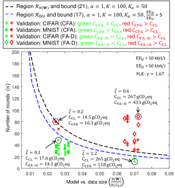
Figure 3: Validation of the bounds (21) in black, and of (17) in blue, with the CIFAR and the MNIST datasets for the CFA and FA-D methods. Markers in the scatter plot report FA-D or CFA simulation runs for the MNIST or CIFAR datasets (IID or non-IID), and give the required rounds for the target loss $\overline{\xi}$ and the corresponding model/data size $\frac{b(\mathbf{W})}{b(\mathcal{E}_{k})}$. Green markers are sustainable solutions, namely $\mathrm{C}_{\mathrm{FA-D}}<\mathrm{C}_{\mathrm{CL}}$ or $\mathrm{C}_{\mathrm{CFA}}<\mathrm{C}_{\mathrm{CL}}$, while red markers refers to the opposite cases.

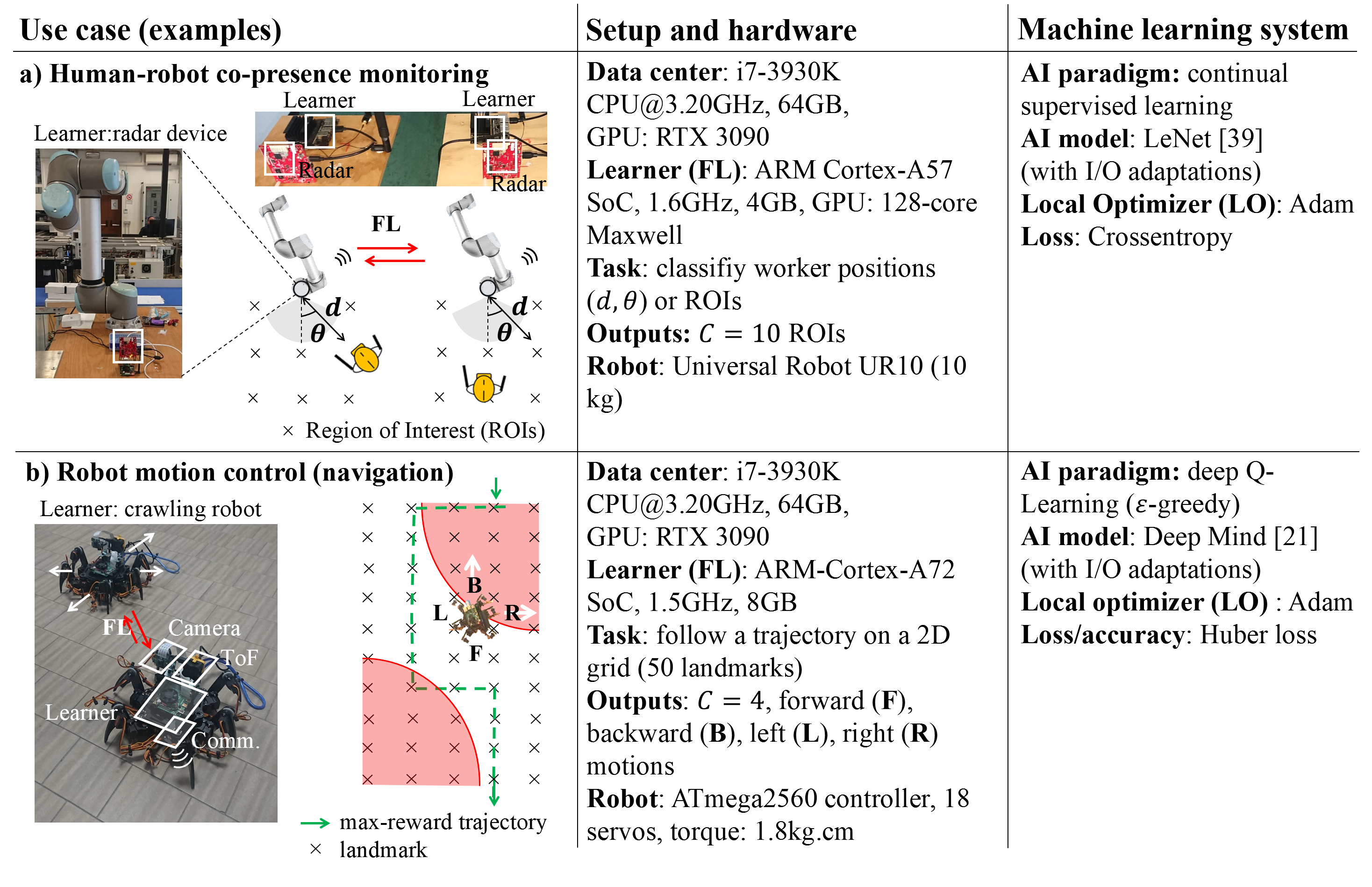
Figure 4: Description of case studies. From left to right: scenario descriptions, hardware specifications for each industrial setup and corresponding ML systems.

V Case studies in industrial IoT

In what follows, we highlight two critical 5G verticals for Industry 4.0 scenarios, further described in Fig. 4. The interested reader might refer to [48] for sustainability requirements in industry processes and transition towards the new Green Deal [49].

The first use case, shown in Fig. 4(a), quantifies the carbon footprint of a continual supervised learning process targeting passive localization of human operators in a shared workplace (human-robot co-presence monitoring). Localization is particularly critical to support various human-robot interactions processes [50] in advanced manufacturing, where robotic manipulators continuously share the same space with humans. A deep ML model is adopted for localization and it is trained continuously to track the variations of data dynamics caused by changes of the workflow processes (typically, on a daily base). In the second setup, described in Fig. 4(b), $K=5$ crawling robots interact with the workplace to learn an optimal sequence of movements and implement a desired trajectory. Robots train a ML model, now via DQL tools [30] as introduced in Sect. II-D. Both case studies focus on industrial setups where AI-based machines/robots are co-located in the same workplace, so that direct communication is possible.

For all case studies, it is assumed that devices have sufficient computing power to implement FL and LO, but they run medium/small-sized deep learning models to allow for real-time operations, i.e., localization or motion control. Hardware and ML systems are described in Fig. 4. The devices, the PS (when used), and the data centers are located in the west EU regions previously defined. In particular, the data center, and the PS are located outside the workplace so that communication is possible only through WWAN connectivity. They are equipped with the same high performance GPU already shown in Sect. IV and have the same PUE namely $\gamma=1.67$. However, a realistic pool of FL learners is considered: manipulator devices are equipped with dedicated hardware modules (Nvidia Jetson Nano) equipped with a low-power GPU (128-core Maxwell architecture) and an ARM Cortex-A57 System-on-Chip (SoC). Crawling robots mount a low-power ARM Cortex-A72 SoC and thus experience larger batch time $T_{k}$ but lower power $P_{k}$ when implementing DQL.

As described in the following, the proposed real-time FL platform adopts MQTT methods for model parameter exchange and several communication profiles. The carbon footprints for both case studies are analyzed separately, while sustainable setups are identified based on the requirements in Table II.

TABLE VI: Summary of main FL parameters for use cases.

	Case (a): Continual Learning		Case (b): Reinforcement Learning
$b\left[\mathcal{E}_{k}(t_{i})\right]$:	$31$ MB ($t_{0}$), $19$ MB ($t_{i}$), $\forall k,i$		$24.6$ MB, $\forall k,i$
$b(\mathbf{W})$:	$1.08$ MB		$5.6$ MB
$\alpha$:	$1$ (1 updates per training, $\forall t_{i}$)		$n$ ($1$ update per round)
$K,K_{a}:$	$K=9,K_{a}:1\sim 9$		$K=5,K_{a}=5$
Consumption	Data center/PS ($k=0$)	Devices ($k\geq 1$)	Data center/PS ($k=0$)	Devices ($k\geq 1$)
$P_{k}$:	$590\,\mathrm{W}$$\,\,(350\,\mathrm{W}$ GPU)	$15\,\mathrm{W}$$(\varphi_{k}=0.36)$	$590\,\mathrm{W}$$\,\,(350\,\mathrm{W}$ GPU)	$5.1\,\mathrm{W}$ $(\varphi_{k}=0.17)$
$T_{k}$:	$10\textrm{ms}$ ($B=3$)	$140\textrm{ms}$ ($B=3$)	$20\textrm{ms}$ ($B=3$)	$400\textrm{ms}$ ($B=3$)
$\beta$:	$0.05$	n.a.	$0.05$	n.a.
$E_{k,\mathrm{sleep}}^{(\mathrm{C})}:$	n.a.	$0.05$ Wh	n.a.	$0.05$ Wh
$\mathrm{EE_{C}:}$	$0.05$ round/J	$0.14$	$\mathrm{EE_{C}}=0.03$ round/J	$0.16$
Peripherals	n.a.	$3$ Wh (radars)	n.a.	$6.6$ Wh (servos)

V-A Networking and MQTT transport

The networking platform used for validation is characterized by $K$ physical IoT devices and implements distributed model training in real-time on top of the MQTT protocol, chosen for low-latency and low-overhead characteristics. For all FL implementations, the exchange of model parameters is performed through MQTT-compliant publish and subscribe operations that are implemented with QoS level 1 [53]. The information included in the MQTT payload are: i) the local model parameters binary encoded with associated meta-information (i.e., the DNN layer type); ii) the FL round; iii) the local loss function used as model quality indicator. The MQTT platform is used to collect measurements of the required training time: the expected carbon footprints are then quantified for varying communication energy efficiencies ($\mathrm{EE_{D}},$ $\mathrm{EE_{U}},$ $\mathrm{EE_{S}}$). The code structure is available in [51]. CL is similarly implemented on top of the same MQTT architecture: in this case, the $K$ devices publish their data to the MQTT broker that is co-located with the data center.

Considering FA and FA-D methods, the PS serves as MQTT broker until the end of the training process: on each FL round, the PS thus accepts subscriptions from the $K_{a}$ active devices that publish their model parameters. For FA method, all the $K$ devices subscribe to the PS broker service, i.e., to download the updated global model. On the other hand, for FA-D, inactive devices need to start a new subscription process every time they wake up from deep-sleep. The $K_{a}$ learners are chosen by a round robin scheduling table [11] that is distributed by the PS at training start, via a dedicated MQTT topic. The broker service might cause an increase of the consumption per round, or a decrease of the computing efficiency $\mathrm{EE_{C}}$. Similarly, subscriptions and publishing operations reduce the communication efficiency, $\mathrm{EE_{D}},$ $\mathrm{EE_{U}}$ depending on the payload-to-overhead ratio of the MQTT messaging [53]. To implement CFA, the MQTT broker is now used to orchestrate the consensus operations, while the PS functions are disabled. Every round, one device is turned on and publishes the local model parameters to a subset of $K_{a}-1$ subscriber devices. Publisher and subscribers are again assigned by round robin scheduling. Notice that the MQTT broker consumption is not considered in this study.

V-B Communication efficiencies

The estimated carbon emissions are quantified by considering $4$ communication efficiency profiles [26] described in the following. The first profile conforms to a LTE design for macro-cell delivery: we set $\mathrm{EE_{U}}=15$ kbit/J and $\mathrm{EE_{D}}=25$ kbit/J as also verified in [40] for a throughput of $28$ Mbps and a BS consumption of $1.35$ kW. Notice that larger efficiency values of $6$ J/Mbit and $10$ J/Mbit for UL and DL, respectively, could be observed with small bulk size of $10$ kB [46]. The second profile corresponds to a NB-IoT implementation. In this case, we set a larger DL $\mathrm{EE_{D}}=50$ kbit/J and UL efficiency of $\mathrm{EE_{U}}=25$ kbit/J. NB-IoT devices also consume about $10$ µW (i.e., $E_{k,\mathrm{sleep}}^{(\mathrm{C})}\simeq 36$ mWh) in deep-sleep mode [47]. The third profile complies with IETF 6TiSCH mesh standard based on IEEE 802.15.4e [52] with a SL efficiency of $\mathrm{EE_{S}}=20$ kbit/J. For the last profile, we adopt a WiFi IEEE 802.11ac implementation, namely the Intel AC 8265 device supporting sidelink connectivity based on Neighbor Awareness Network [54]. Typical communication efficiencies are $2100$ mW/Mbps for receiving and $2500$ mW/Mbps for transmitting [29]; however, they do not include equipment consumption, nor WiFi and MQTT overheads: the assumed SL efficiency is thus $\mathrm{EE_{S}}=100$ kbit/J. Notice that sidelink efficiency is expected to scale up to at least $10$ times in 6G implementations [26].

V-C Human-robot interaction: continual learning

The goal of the training task is to learn a ML model for the detection (i.e., classification) of the position of the human operators sharing the workspace, namely the human-robot distance $d$ and the direction of arrival (DOA) $\theta$. In particular, we address the detection of a human subject in $C=10$ Region Of Interest (ROI), including the one referring to the subject outside the monitored area: ROIs are detailed in Fig. 4(a). The proposed training scenario resorts to a network of $K=9$ physical devices where each one is equipped with a Time-Division Multiple-Input-Multiple Output (TD-MIMO) Frequency Modulated Continuous Wave (FMCW) radar working in the $77-81$ GHz band. For details about the robotic manipulators, the industrial environment and the radars, the interested reader may also refer to [50]. Radars use a trained deep learning model to obtain position ($d$, $\theta$) information and the corresponding ROI. In addition, the subject position can be sent to a programmable logic controller for robot safety control, for emergency stop or replanning tasks. The ML model adopted for the classification of the operator location is the LeNet-4 scheme, proposed in [22] with input adaptations, that consists of $4$ trainable layers and $28$K parameters. Model footprint is $b(\mathbf{W})=1.08$ MB, the other parameters are detailed in Tab. VI.

The FL system implements a continual learning task (Sect. II-D): at time $t_{0}$, each device collects a large dataset $\mathbf{x}_{h}$ of raw range-azimuth data manually labelled, with size $b[\mathcal{E}_{k}(t_{0})]=31$ MB. This set is used for initial training of the ML model. Re-training stages, $t_{i}$, $i>0$, are based on new data, $b[\mathcal{E}_{k}(t_{i})]=19$ MB, collected on a daily basis. Datasets for initial model training and $2$ subsequent example re-training stages, $t_{1},t_{2}$, are available online in [51]. To simplify the analysis, in what follows, we compared the results of the proposed FA-D and CFA implementations, while FA is not considered. For FA-D, the number of active devices ranges from $K_{a}=1$ to $K_{a}=9$; for CFA, we have assumed $K_{a}=3$ ($1$ publisher, $2$ subscribers per round) up to $K_{a}=9$ ($1$ publisher, $8$ subscribers per round).

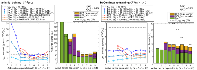
Figure 5: Continual learning case study. From left to right: (a) carbon footprints $\mathrm{C}^{(t_{0})}(n_{0})$ and corresponding number of FL rounds ($n_{0}$) during initial training stage $t_{0}$, for varying population of active learners $K_{a}=1\sim 9$ and $K=9$ radars; (b) carbon footprints $\mathrm{C}^{(t_{i})}(n_{i})$ and corresponding rounds $(n_{i})$ averaged over $2$ subsequent re-training stages ($i=1,2$). For all cases, footprints are evaluated for CL (dashed line), CFA (cross markers), and FA-D (diamond markers) as well as $4$ communication efficiency profiles that comply with LTE, NB-IoT, IEEE 802.15.4e and WiFi IEEE 802.11.ac implementations. Rounds $(n_{i})$ and learners $(K_{a})$ are compared with bound (21) obtained using the parameters of Tab. VI.

Selection of the device population ($K_{a}$). The example in Fig. 5 uses the requirements in Table II as a guideline for the selection of the smallest population size $K_{a}$, so that FL emits lower carbon than CL during initial ($i=0$) and re-training ($i>0$) stages. The figure highlights the carbon footprints and the number of rounds for both stages. In particular, Fig. 5(a) highlights the carbon footprints $\mathrm{C}^{(t_{0})}$ and the number of learning rounds $n_{0}$ that are measured during the initial training phase ($t_{0}$) for varying number of active learners $K_{a}$. Fig. 5(b) shows the same results, namely $\mathrm{C}^{(t_{i})}$ and $n_{i}$, averaged over the subsequent re-training stages, $i=1,2$. The target loss is here $\overline{\xi}=0.1$ for all cases.

Considering the initial training first, FA-D and CFA implemented over small population sets, i.e., $K_{a}\leq 3$, need a large number of rounds ($n>150$) and training time. Bound (21) for region $\mathcal{R}_{b(\mathbf{W})}$ gives some practical guidelines for optimizing $K_{a}$ population. For $\frac{b(\mathbf{W})}{b(\mathcal{E}_{k})}\simeq 0.035$, since $b[\mathcal{E}_{k}(t_{0})]=31$ MB, and the other parameters in Tab. VI, the requirement (21) becomes $K_{a}<\tfrac{257}{n}$. Considering CFA, the minimum population size that satisfies (21) is $K_{a}=6$ since $n_{\mathrm{CFA}}=40$ rounds. Larger populations, i.e., $K_{a}\geq 8$, increase the cost per round, with no significant savings in terms of training time. $K_{a}=4$ can be chosen for FA-D as $n_{\mathrm{FA-D}}=40$ rounds. Using (17) for $K_{a}=4$, the required DL efficiency should comply with $\mathrm{\tfrac{EE_{D}}{EE_{U}}>6.2}$: on the other hand, since condition on computing cost (23) is satisfied for $\mathrm{CI}_{k}=0.97$ and $\varphi_{k}=0.36$, as $K_{a}\cdot\tfrac{0.36}{0.95}<1.67$, a lower DL efficiency can be tolerated.

Focusing now on model re-training stage, FA-D and CFA leave a smaller footprint than CL for all choices of $K_{a}$ as they need few rounds ($<20$) for model update. With $\frac{b(\mathbf{W})}{b(\mathcal{E}_{k})}\simeq 0.057$, since now $b[\mathcal{E}_{k}(t_{i})]=19$ MB, the requirement (21) for FA-D becomes $K_{a}<\tfrac{158}{n}$ and it is satisfied for $K_{a}=1$ as $n_{\mathrm{FA-D}}<12$. For CFA, it is $K_{a}=3$ since $n_{\mathrm{CFA}}<20$. For example, FA-D with only $K_{a}=1$ learner per round emits $1.1$ gCO2-eq per re-training stage (over LTE networks), which corresponds to a carbon emission of $0.4$ kgCO2-eq per year, assuming $1$ re-training/day. For the same setup, CL would cost $5.4$ gCO2-eq, corresponding to roughly to $2$ kgCO2-eq per year.

To sum up, the results suggest that both FA-D and CFA are sustainable choices for re-training, as they avoid unnecessary data uploads. On the other hand, for initial training, CL and FL are both competitive and should be considered carefully based on the available communication interface and sustainability conditions (17)-(23). Notice that the availability of low-power sidelink communications makes CFA the preferred choice.

V-D Reinforcement learning for robot motion planning

According to the scenario of Fig. 4(b) and the parameters of Tab. VI, the considered RL setting features $K=5$ networked robots that collaboratively learn an optimized sequence of motions, to follow an assigned trajectory, highlighted in green. Since the goal is to quantify the carbon footprint of the distributed learning processes against CL in a realistic setup, the motion control problem is simplified by letting the robots move on a 2D regular grid space consisting of $40$ landmark points, while the action space consists of $4$ motions: Forward (F), Backward (B), Left (L), and Right (R). Each robot explores a different site area collecting new training data in real-time: data are obtained from two cameras, namely a standard RGB camera and a short-range Time Of Flight (TOF) one [55]. Exploration of the environment and training data collection is responsible for additional energy consumption (quantified here as $6.6$ Wh) that depends on robot/servos hardware.

RL and DeepMind model [21] are used to train a policy that maps observations of the workplace to a set of actions, namely robot motions, while trying to maximize a long-term reward. Exploration and model exploitation follow the $\varepsilon$-greedy method while, in this example, exploration takes $20$ robot motions for each learning round. DeepMind model consists of $5$ trainable layers and $1.3$M parameters: model footprint from MQTT payload is $b(\mathbf{W})=5.6$ MB. Notice that for CL the training data is moved on every round, therefore $\alpha=n$. CFA and FA are considered here with the setup highlighted in Sect. II-D, with $K_{a}=K$. Data footprint is $b(\mathcal{E}_{k})=24.6$ MB, therefore $\frac{b(\mathbf{W})}{b(\mathcal{E}_{k})}\simeq 0.23$: with such setup, condition (21) for RL is satisfied and requirement for region $\mathcal{R}_{b(\mathbf{W})}$ becomes $\frac{b(\mathbf{W})}{b(\mathcal{E}_{k})}<\frac{K}{K_{a}}$.

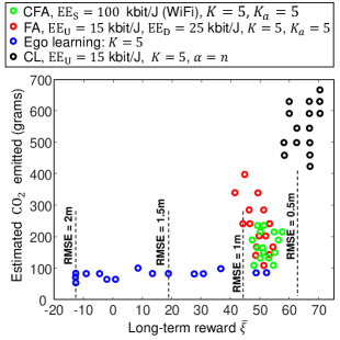
Figure 6: Reinforcement Learning for robot navigation: estimated CO2 emissions for each policy optimization vs the running reward. Each reward value corresponds to an average trajectory error compared with the desired one, measured by root mean squared error (RMSE). Specific parameters are in Tab. VI. CL is in black, FA in red, CFA in green and ego learning in blue. Each point of the scatter plot represents one simulation episode.

Impact of target reward/accuracy. Fig. 6 shows the estimated carbon emissions versus the obtained reward considering CL (black), FA (red), CFA (green) and ego learning (blue) policies. For the opportunistic/ego learning approach [2], the robots disable the radio interface and train their local models using the training data from on-board sensors only. Each point in the scatter plot of Fig. 6 corresponds to the carbon footprint measured in one simulation episode. On each new episode, the observed footprint might vary due to the random exploration phase. In ego learning, the robots explore the environment for a longer time, thus training takes around $25$ h corresponding to $4500\sim 5000$ rounds since servos need $1$ s per motion. For comparison, CL takes $90$ minutes on average ($250\sim 300$ rounds), while FA needs $180$ minutes ($500\sim 550$ rounds) and CFA $150$ minutes ($400\div 450$ rounds).

RL generally requires more rounds than continual learning to converge, and cause large emissions when considering the whole training process. Ego learning gives the lowest footprint as consumption is only due to the robot and the LO. However, it experiences lower rewards, from $-10$ to $30$ as the learned trajectory is far from the desired one, with corresponding Root Mean Squared Errors (RMSE) between $1.5$ m and $2$ m. CL converges faster at the cost of a large footprint, about $2$ times larger than FA/CFA and $6$ times larger than ego learning. However, rewards are close to $70$, that corresponds to learned trajectories with RMSE $0.5$ m. Compared with CL, FA and CFA performance are now close since all robots are active; energy savings are obtained at the cost of rewards penalties, scaling down to $40\sim 60$, with RMSE between $0.5$ m and $1$ m. Considering ego and CL as extreme cases, where the former gives low-accuracy and small footprint, while the latter high-accuracy and large footprint, FL is a promising tradeoff solution, as trading accuracy (reward) with environmental footprint.

VI Conclusions

The article proposed a novel framework for the analysis of energy and carbon footprints in distributed and federated learning. A tradeoff analysis was characterized for vanilla FL and decentralized, consensus-driven learning, compared with centralized training. The analyzed algorithms are suitable for low-power embedded wireless devices with constrained memory, typically adopted in industrial IoT processes requiring low latency. The paper also explored operational conditions applicable to both conventional FL methods and generalized distributed learning policies targeting carbon-efficiency. Minimal requirements for FL are obtained analytically and have been applied in different scenarios to steer the choice towards sustainable designs.

Carbon equivalent emissions have been analyzed for two industry relevant 5G verticals, using real datasets and a test-bed characterized by physical IoT devices implementing real-time model training on top of the MQTT transport, tailored to support various learning processes. For each considered case, centralized versus distributed training impact is discussed for continual and reinforcement learning problems. Sustainability of the FL depends in many cases on model vs data footprints, as well as the population of active devices, that must be selected to balance energy budget and training data quality. Downlink vs uplink (or sidelink) communication efficiency and the amount of available green energy are additional key factors. The proposed CFA and FA with deep sleep mode (FA-D) methods have been shown to be effective as they minimize the number of active learners at each learning round. The selection of the learner population size according to the proposed design patterns provides significant savings per round ($20\%\sim 30\%$ and higher) compared with baselines. CFA has an advantage over FA-D provided that an efficient sidelink communication interface is available: the co-design of learning and communication is thus of high importance. Finally, the energy footprints of reinforcement learning need much more careful considerations than conventional supervised learning, due to the considerable carbon emissions. Results indicate that FL is a promising solution as it trades off energy and accuracy compared with the extreme cases of ego (low rewards/footprint) and centralized training (high rewards/footprint).

Appendix

Communication costs: FA and FA-D design constraints

Using the carbon footprints shown in Tab. I, the constraint $\mathrm{C}_{\mathrm{FA}}^{(\mathrm{C})}<\mathrm{C}_{\mathrm{CL}}^{(\mathrm{C})}$ in region $\mathcal{R}_{\mathrm{DU}}$ (16) implies that, after straightforward manipulation, the following condition has to be met

$$\mathrm{\frac{EE_{D}}{\mathrm{EE}_{\mathrm{U}}}\cdot}\left[\mathcal{\mathcal{H}}\left(\frac{b(\mathbf{W})}{b(\mathcal{E})}\right)-\frac{1}{K_{a}}\sum_{k=1}^{K_{a}}\mathrm{CI}_{k}\right]>\gamma\cdot\frac{K}{K_{a}}\mathrm{CI}_{0}$$ (24)

with

$$\mathcal{\mathcal{H}}\left(\frac{b(\mathbf{W})}{b(\mathcal{E})}\right)=\frac{\alpha}{n\cdot K_{a}}\frac{b(\mathcal{E})}{b(\mathbf{W})}\sum_{k=1}^{K}\sigma_{k}\mathrm{CI}_{k}$$ (25)

where $\sigma_{k}$, defined in (5) with $\sum_{k=1}^{K}\sigma_{k}=1,$ counts the number of the local ($k$) examples out of the number of the global ones, respectively. Eq. (17) is then obtained by setting $\mathrm{CI}_{k}=\mathrm{CI}$, $\forall k$. Considering FA-D, the equation (24) becomes $\mathrm{\frac{EE_{D}}{\mathrm{EE}_{\mathrm{U}}}\cdot}\mathcal{\mathcal{H}}\left(\frac{b(\mathbf{W})}{b(\mathcal{E})}\right)>\gamma\mathrm{CI}_{0}$.

For $\mathrm{\frac{EE_{D}}{\mathrm{EE}_{\mathrm{U}}}}$ large enough as assumed for derivation of region $\mathcal{R}_{b(\mathbf{W})}$ in problem (20), the condition $\max[\mathrm{C}_{\mathrm{FA}}^{(\mathrm{C})},\mathrm{C}_{\mathrm{FA-D}}^{(\mathrm{C})}]<\mathrm{C}_{\mathrm{CL}}^{(\mathrm{C})}$ is guaranteed as long as

$$\mathcal{\mathcal{H}}\left(\frac{b(\mathbf{W})}{b(\mathcal{E})}\right)>\frac{1}{K_{a}}\sum_{k=1}^{K_{a}}\mathrm{CI}_{k},$$ (26)

that corresponds to

$$\frac{b(\mathbf{W})}{b(\mathcal{E})}\cdot K<\frac{\alpha}{n}\cdot\frac{\sum_{k=1}^{K}\sigma_{k}\mathrm{CI}_{k}}{\sum_{k=1}^{K_{a}}\mathrm{CI}_{k}}.$$ (27)

Constraint (27) can be further simplified by letting, $\forall k,$ $\sigma_{k}\simeq 1/K,$ namely $b(\mathcal{E}_{k})\simeq\frac{b(\mathcal{E})}{K}$, and $\mathrm{CI}_{k}=\mathrm{CI}$, to obtain (21) with $\Gamma=1$.

Communication costs: CFA design constraints

Using Tab. I and (25), the constraint $\mathrm{C}_{\mathrm{CFA}}^{(\mathrm{C})}<\mathrm{C}_{\mathrm{CL}}^{(\mathrm{C})}$ for region (18) results in

$$\frac{\mathrm{EE_{S}}}{\mathrm{EE}_{\mathrm{U}}}\cdot\mathcal{\mathcal{H}}\left(\frac{b(\mathbf{W})}{b(\mathcal{E})}\right)>\frac{N}{K_{a}}\sum_{k=1}^{K_{a}}\mathrm{CI}_{k}$$ (28)

that simplifies to (19) when, $\forall k$, it is $b(\mathcal{E}_{k})\simeq\frac{b(\mathcal{E})}{K}$, and $\mathrm{CI}_{k}=\mathrm{CI}$. Furthermore,

$$\mathrm{\frac{EE_{S}}{\mathrm{EE_{U}}}}+\gamma\cdot K\cdot\frac{\mathrm{CI}_{0}}{\sum_{k=1}^{K_{a}}\mathrm{CI}_{k}}\cdot\mathrm{\frac{EE_{S}}{\mathrm{EE_{D}}}}>N$$ (29)

guarantees lower carbon footprint per round than FA, namely $\frac{\mathrm{C}_{\mathrm{CFA}}^{(\mathrm{C})}}{n_{\mathrm{CFA}}}<\frac{\mathrm{C}_{\mathrm{FA}}^{(\mathrm{C})}}{n_{\mathrm{FA}}}.$ The comparison of CFA vs FA-D gives the same result shown in (29) but a more stringent condition as $K$ must be replaced with $K_{a}$. As expected, considering an individual round, CFA footprint is closer to FA-D as both strategies target the minimization of the active device population.

In WWAN, or cellular settings, D2D connectivity is replaced by UL and DL communications, namely $[\mathrm{EE}_{\mathrm{S}}]^{-1}=[\mathrm{EE}_{\mathrm{D}}]^{-1}+[\mathrm{EE}_{\mathrm{U}}]^{-1}$. In this case the constraint (28) becomes

$$\frac{\mathrm{EE_{D}}}{\mathrm{EE}_{\mathrm{U}}}\cdot\left[\mathcal{\mathcal{H}}\left(\frac{b(\mathbf{W})}{b(\mathcal{E})}\right)-\frac{N}{K_{a}}\sum_{k=1}^{K_{a}}\mathrm{CI}_{k}\right]>\frac{N}{K_{a}}\cdot\sum_{k=1}^{K_{a}}\mathrm{CI}_{k},$$ (30)

while for $\mathrm{\frac{EE_{D}}{\mathrm{EE}_{\mathrm{U}}}}$ large enough, sustainability is guaranteed as long as

$$\mathcal{\mathcal{H}}\left(\frac{b(\mathbf{W})}{b(\mathcal{E})}\right)>\frac{N}{K_{a}}\sum_{k=1}^{K_{a}}\mathrm{CI}_{k}.$$ (31)

Comparing (26) with (31), the condition $\max[\mathrm{C}_{\mathrm{CFA}}^{(\mathrm{C})},\mathrm{C}_{\mathrm{FA}}^{(\mathrm{C})},\mathrm{C}_{\mathrm{FA-D}}^{(\mathrm{C})}]<\mathrm{C}_{\mathrm{CL}}^{(\mathrm{C})}$ for the derivation of region $\mathcal{R}_{b(\mathbf{W})}$ in (20), can be rewritten as in (31). Finally, replacing $\forall k$ $\mathrm{CI}_{k}=\mathrm{CI}$, we obtain (21) now with $\Gamma=N$.

References

- [1] M. Dayarathna, et al., “Data Center Energy Consumption Modeling: A Survey,” IEEE Communications Surveys & Tutorials, vol. 18, no. 1, pp. 732–794, First quarter 2016.
- [2] S. Savazzi, et al., “Opportunities of Federated Learning in Connected, Cooperative and Automated Industrial Systems,” IEEE Communications Magazine, vol. 59, no. 2, pp. 16–21, Feb. 2021.
- [3] X. Qiu, et al., “A first look into the carbon footprint of federated learning,” 2021. [Online]. Available: https://arxiv.org/abs/2102.07627
- [4] P. Kairouz et al., “Advances and open problems in federated learning,” Foundations and Trends in Machine Learning, Now Publishers, 2021. [Online]. Available: https://arxiv.org/abs/1912.04977.
- [5] J. Konečný, et al., “Federated optimization: Distributed machine learning for on-device intelligence,” CoRR, 2016. [Online]. Available: http://arxiv.org/abs/1610.02527.
- [6] H. B. McMahan, et al., “Communication-efficient learning of deep networks from decentralized data,” Proc. of the 20th Int. Conf. on Artificial Intelligence and Statistics (AISTATS’17), Fort Lauderdale, Florida, USA, pp. 1–10, 2017.
- [7] L. U. Khan, et al., “Federated Learning for Internet of Things: Recent Advances, Taxonomy, and Open Challenges,” IEEE Communications Surveys & Tutorials, to appear, 202l.
- [8] R. Yu, P. Li, “Toward Resource-Efficient Federated Learning in Mobile Edge Computing,” IEEE Network, vol. 35, no. 1, pp. 148–155, January/February 2021.
- [9] M. M. Amiri, et al., “Federated learning over wireless fading channels,” IEEE Trans. Wireless Commun., vol. 19, no. 5, pp. 3546–3557, May 2020.
- [10] Z. Yang, et al. “Energy Efficient Federated Learning Over Wireless Communication Networks,” IEEE Transactions on Wireless Communications, vol. 20, no. 3, pp. 1935-1949, March 2021.
- [11] H. H. Yang, et al., “Scheduling Policies for Federated Learning in Wireless Networks,” IEEE Transactions on Communications, vol. 68, no. 1, pp. 317-333, Jan. 2020.
- [12] A. Reisizadeh, et al. “FedPAQ: A communication-efficient federated learning method with periodic averaging and quantization,” Proc. Int. Conf. Artif. Intell. Statist., pp. 2021–2031, 2020. [Online]. Available: https://arxiv.org/abs/1909.13014.
- [13] A. Elgabli, et al., “GADMM: Fast and Communication Efficient Framework for Distributed Machine Learning,” Journal of Machine Learning Research, vol. 21, no. 76, pp. 1–39, 2020.
- [14] M. Mohammadi Amiri and D. Gündüz, “Machine Learning at the Wireless Edge: Distributed Stochastic Gradient Descent Over-the-Air,” IEEE Transactions on Signal Processing, vol. 68, pp. 2155-2169, 2020.
- [15] M. Blot, et al., “Gossip training for deep learning,” 30th Conference on Neural Information Processing Systems (NIPS), Barcelona, Spain, 2016. [Online]. Available: https://arxiv.org/abs/1611.09726.
- [16] S. Savazzi, et al., “Federated Learning with Cooperating Devices: A Consensus Approach for Massive IoT Networks,” IEEE Internet of Things Journal, vol. 7, no. 5, pp. 4641–4654, May 2020.
- [17] H. Xing, et al., “Federated Learning Over Wireless Device-to-Device Networks: Algorithms and Convergence Analysis,” IEEE Journal on Selected Areas in Communications, vol. 39, no. 12, pp. 3723-3741, Dec. 2021.
- [18] Z. Chen, et al., “Consensus-Based Distributed Computation of Link-Based Network Metrics,” IEEE Signal Processing Letters, vol. 28, pp. 249–253, 2021.
- [19] W. Saad, et al., “A Vision of 6G Wireless Systems: Applications, Trends, Technologies, and Open Research Problems,” IEEE Network, vol. 34, no. 3, pp. 134–142, May/June 2020.
- [20] S. Savazzi, et al., “A Framework for Energy and Carbon Footprint Analysis of Distributed and Federated Edge Learning,” Proc. IEEE Personal Indoor Mobile Radio Communications (PIMRC), 2021. [Online]. Available: https://arxiv.org/abs/2103.10346.
- [21] K. Arulkumaran, et al. “Deep Reinforcement Learning: A Brief Survey,” IEEE Signal Processing Magazine, vol. 34, no. 6, pp. 26–38, Nov. 2017.
- [22] G. Cohen, et al., “EMNIST: Extending MNIST to handwritten letters,” Proc. Int. Joint Conf. Neural Netw., pp. 2921–2926, May 2017.
- [23] A. Krizhevsky, et al., “Cifar-10 (canadian institute for advanced research).” [Online]. Available: https://www.cs.toronto.edu/~kriz/cifar.html.
- [24] W. Liu, et al., “Decentralized federated learning: Balancing communication and computing costs,” IEEE Transactions on Signal and Information Processing over Networks, vol. 8, pp. 131–143, 2022.
- [25] L. Barbieri, et al., “Decentralized federated learning for extended sensing in 6G connected vehicles,” Vehicular Communications, vol. 33, 100396, 2022.
- [26] David Lopez-Perez, et al., “A Survey on 5G Energy Efficiency: Massive MIMO, Lean Carrier Design, Sleep Modes, and Machine Learning,” 2021. [Online]. Available: https://arxiv.org/abs/2101.11246.
- [27] H. Guo, et al., “Analog Gradient Aggregation for Federated Learning Over Wireless Networks: Customized Design and Convergence Analysis,” IEEE Internet of Things Journal, vol. 8, no. 1, pp. 197-210, 1 Jan., 2021.
- [28] Tian Li, et al., “Federated Optimization in Heterogeneous Networks,” Proceedings of the 3 rd MLSys Conference, Austin, TX, USA, 2020. [Online]. Available: https://arxiv.org/abs/1812.06127.
- [29] M. Höyhtyä, et al., “Review of latest advances in 3GPP standardization: D2D communication in 5G systems and its energy consumption models,” Future Internet, vol. 10, no. 1, 2018.
- [30] V. Mnih, et al., “Human-level control through deep reinforcement learning,” Nature 518, pp. 529–533, 2015.
- [31] E. Masanet, et al., “Characteristics of low-carbon data centres,” Nature Climate Change, vol. 3, no. 7, pp. 627–630, 2013.
- [32] A. Capozzoli, et al., “Cooling systems in data centers: state of art and emerging technologies,” Energy Procedia, vol. 83, pp. 484–493, 2015.
- [33] C. Finn, et al. “Model-Agnostic Meta-Learning for Fast Adaptation of Deep Networks,” in Proc. 34th International Conference of Machine Learning (ICML), pp. 1126–1135, 2017.
- [34] O. Simeone, et al., “From Learning to Meta-Learning: Reduced Training Overhead and Complexity for Communication Systems,” Proc. 2020 2nd 6G Wireless Summit, Lapland, Finland, Mar. 2020. [Online]. Available https://arxiv.org/abs/2001.01227
- [35] A. Rajeswaran, et al. “Meta-Learning with Implicit Gradients,” in Proc. of 33rd Conference on Neural Information Processing Systems (NeurIPS), 2019.
- [36] L.F.W. Anthony, et al., “Carbontracker: Tracking and Predicting the Carbon Footprint of Training Deep Learning Models,” Proc of ICML Workshop on Challenges in Deploying and monitoring Machine Learning Systems, 2020.
- [37] European Environment Agency, Data and maps: “Greenhouse gas emission intensity of electricity generation,” Dec. 2020. [Online]. Available: https://tinyurl.com/36l5v5ht
- [38] ETSI TC EE, “ES 203 228, Environmental Engineering (EE); Assessment of mobile network energy efficiency,” V1.3.1, Oct. 2020.
- [39] G. Auer, et al., “How much energy is needed to run a wireless network?,” IEEE Wireless Communications, vol. 18, no. 5, pp. 40–49, October 2011.
- [40] E. Björnson, E. G. Larsson, “How Energy-Efficient Can a Wireless Communication System Become?,” Proc. 52nd Asilomar Conf. on Sig., Syst., and Comp., Pacific Grove, CA, USA, pp. 1252–1256, 2018.
- [41] T. Huang, et al., “A Survey on Green 6G Network: Architecture and Technologies,” IEEE Access, vol. 7, pp. 175758–175768, 2019.
- [42] M. Giordani, et al., “Toward 6G Networks: Use Cases and Technologies,” IEEE Communications Magazine, vol. 58, no. 3, pp. 55–61, Mar. 2020
- [43] J. G. J. Olivier, et al., “Trend in global CO2 and total greenhouse gas emissions,” 2020 Report, PBL Netherland Environmental Assessment Agency, Dec. 2020. [Online]. Available: https://tinyurl.com/xzz7btj6.
- [44] A. Lacoste, et al., “Quantifying the Carbon Emissions of Machine Learning,” [Online]. Available: http://arxiv.org/abs/1910.09700.
- [45] H. Fekete, et al., “A review of successful climate change mitigation policies in major emitting economies and the potential of global replication,” Renewable and Sustainable Energy Reviews, vol. 137, art. 110602, 2021.
- [46] J. Huang, et al., “A close examination of performance and power characteristics of 4G LTE networks,” Proc. of the 10th international conference on Mobile Systems, Applications, and Services, pp. 225–238, Jun. 2012.
- [47] F. Michelinakis, et al., “Dissecting Energy Consumption of NB-IoT Devices Empirically,” IEEE Internet of Things Journal, vol. 8, no. 2, pp. 1224–1242, 15 Jan.15, 2021. [Online]. Available. https://arxiv.org/abs/2004.07127.
- [48] L. B. Furstenau et al., “Link Between Sustainability and Industry 4.0: Trends, Challenges and New Perspectives,” IEEE Access, vol. 8, pp. 140079–140096, 2020.
- [49] K. Neuhoff, et al., “Green Deal for industry: A clear policy framework is more important than funding,” DIW Weekly Report, vol. 11, no. 10, pp. 73–82, 2021.
- [50] S. Kianoush, et al., “A Multisensory Edge-Cloud Platform for Opportunistic Radio Sensing in Cobot Environments,” IEEE Internet of Things Journal, vol. 8, no. 2, pp. 1154–1168, 2021.
- [51] S. Savazzi, “Federated Learning: mmWave MIMO radar dataset for testing”, IEEE Dataport, doi: https://dx.doi.org/10.21227/0wmc-hq36. [Online] Available: http://ieee-dataport.org/2312. Accessed: 03/08/2021.
- [52] X. Vilajosana, et al., “IETF 6TiSCH: A Tutorial,” IEEE Communications Surveys & Tutorials, vol. 22, no. 1, pp. 595–615, Firstquarter 2020.
- [53] L. Mainetti, et. al., “A Software Architecture Enabling the Web of Things,” IEEE Internet of Things Journal, vol. 2, no. 6, pp. 445–454, 2015.
- [54] D. Camps-Mur, et al., “Enabling always on service discovery: Wifi neighbor awareness networking,” IEEE Wireless Communications, vol. 22, no. 2, pp. 118–125, April 2015.
- [55] Terabee, Teraranger EVO 64px, Technical Specifications, Terabee, 2018. [Online]. Available: https://tinyurl.com/vaz79xs. Accessed: Aug. 2021.