Parameter estimation for a linear parabolic SPDE model
in two space dimensions with a small noise

Abstract.

We study parameter estimation for a linear parabolic second-order stochastic partial differential equation (SPDE) in two space dimensions with a small dispersion parameter using high frequency data with respect to time and space. We set two types of $Q$-Wiener processes as a driving noise. We provide minimum contrast estimators of the coefficient parameters of the SPDE appearing in the coordinate process of the SPDE based on the thinned data in space, and approximate the coordinate process based on the thinned data in time. Moreover, we propose an estimator of the drift parameter using the fact that the coordinate process is the Ornstein-Uhlenbeck process and statistical inference for diffusion processes with a small noise.

1. Introduction

We deal with the following linear parabolic stochastic partial differential equation (SPDE) in two space dimensions

$$\mathrm{d}X_{t}^{Q}(y,z) =\biggl{\{}\theta_{2}\biggl{(}\frac{\partial^{2}}{\partial y^{2}}+\frac{\partial^{2}}{\partial z^{2}}\biggr{)}+\theta_{1}\frac{\partial}{\partial y}+\eta_{1}\frac{\partial}{\partial z}+\theta_{0}\biggr{\}}X_{t}^{Q}(y,z)\mathrm{d}t$$

$$\qquad+\epsilon\mathrm{d}W_{t}^{Q}(y,z),\quad(t,y,z)\in[0,1]\times D,$$ (1.1)

$$X_{0}^{Q}(y,z) =\xi(y,z),\quad(y,z)\in D,$$

$$X_{t}^{Q}(y,z) =0,\quad(t,y,z)\in[0,1]\times\partial D,$$

where $D=[0,1]^{2}$, $\epsilon\in(0,1]$ is a known small dispersion parameter, $W_{t}^{Q}$ is a $Q$-Wiener process in a Sobolev space on $D$, an initial value $\xi$ is independent of $W_{t}^{Q}$, $\theta=(\theta_{0},\theta_{1},\eta_{1},\theta_{2})$ is an unknown parameter and $(\theta_{0},\theta_{1},\eta_{1},\theta_{2})\in\mathbb{R}^{3}\times(0,\infty)$. Moreover, the parameter space $\Theta$ is a compact convex subset of $\mathbb{R}^{3}\times(0,\infty)$, $\theta^{*}=(\theta_{0}^{*},\theta_{1}^{*},\eta_{1}^{*},\theta_{2}^{*})$ is the true value of $\theta$ and we assume that $\theta^{*}\in\mathrm{Int}\,\Theta$. The data are discrete observations $\{X_{t_{i}}^{Q}(y_{j_{1}},z_{j_{2}})\}$, $i=0,\ldots,N$, $j_{1}=0,\ldots,M_{1}$, $j_{2}=0,\ldots,M_{2}$, $M=M_{1}M_{2}$ with $t_{i}=i/N$, $y_{j_{1}}=j_{1}/M_{1}$ and $z_{j_{2}}=j_{2}/M_{2}$.

SPDEs have been applied in various fields such as physics, engineering, and economics. For instance, a stochastic heat equation is a family of our model, a linear parabolic SPDE, and is a basic and important model that appears in many situations. For application of linear parabolic SPDEs, see Piterbarg and Ostrovskii [27], which dealt with sea surface temperature variability.

Statistical inference for SPDE models has been developed by many researchers. For an overview of existing theories, see Lototsky [23] and Cialenco [4]. As for discrete observations, see Markussen [25], Bibinger and Trabs [1], Chong [3], [2], Cialenco et al. [5], Cialenco and Huang [7], Hildebrandt [13], Kaino and Uchida [18], [19], Hildebrandt and Trabs [15], [14], Tonaki et al. [30] and references therein. Recently, Kaino and Uchida [19] considered the following linear parabolic SPDE model in one space dimension

$$\mathrm{d}X_{t}(y) =\biggl{(}\theta_{2}\frac{\partial^{2}}{\partial y^{2}}+\theta_{1}\frac{\partial}{\partial y}+\theta_{0}\biggr{)}X_{t}(y)\mathrm{d}t+\epsilon\mathrm{d}B_{t}(y),\quad(t,y)\in[0,T]\times[0,1],$$ (1.2)

$$X_{0}(y) =\xi(y),\quad y\in[0,1],\qquad X_{t}(0)=X_{t}(1)=0,\quad t\in[0,T],$$

where $\epsilon\in(0,1]$ is a known small dispersion parameter, $T>0$, $B_{t}$ is a cylindrical Brownian motion in a Sobolev space on $[0,1]$, $\xi$ is an initial value and $\theta_{0},\theta_{1},\theta_{2}$ are unknown parameters. They proposed the adaptive maximum likelihood type estimation for the coefficient parameters $\theta_{0}$, $\theta_{1}$ and $\theta_{2}$, and then showed that the estimators of $\theta_{0}$, $\theta_{1}$ and $\theta_{2}$ are asymptotically normal. Tonaki et al. [30] studied the following linear parabolic SPDE in two space dimensions

$$\mathrm{d}\bar{X}_{t}^{Q}(y,z) =\biggl{\{}\theta_{2}\biggl{(}\frac{\partial^{2}}{\partial y^{2}}+\frac{\partial^{2}}{\partial z^{2}}\biggr{)}+\theta_{1}\frac{\partial}{\partial y}+\eta_{1}\frac{\partial}{\partial z}+\theta_{0}\biggr{\}}\bar{X}_{t}^{Q}(y,z)\mathrm{d}t$$

$$\qquad+\sigma\mathrm{d}W_{t}^{Q}(y,z),\quad(t,y,z)\in[0,1]\times D,$$ (1.3)

$$\bar{X}_{0}^{Q}(y,z) =\xi(y,z),\quad(y,z)\in D,$$

$$\bar{X}_{t}^{Q}(y,z) =0,\quad(t,y,z)\in[0,1]\times\partial D,$$

where $D=[0,1]^{2}$, $W_{t}^{Q}$ is a $Q$-Wiener process in a Sobolev space on $D$, $\xi$ is an initial value, $(\theta_{0},\theta_{1},\eta_{1},\theta_{2})$ and $\sigma$ are unknown parameters and $(\theta_{0},\theta_{1},\eta_{1},\theta_{2},\sigma)\in\mathbb{R}^{3}\times(0,\infty)^{2}$. Since a mild solution $\bar{X}_{t}^{I}$ of the SPDE (1.3) driven by a cylindrical Brownian motion $B_{t}=W_{t}^{I}$ ($I$ is the identity operator) is not square integrable for a.e. $(t,y,z)\in[0,1]\times D$ (see Remark 1 in [30]), they considered two types of $Q$-Wiener processes given by (2.1) and (2.2) below. They showed consistency and asymptotic normality for the estimators of $(\theta_{0},\theta_{1},\eta_{1},\theta_{2},\sigma^{2})$ when the driving noise is a $Q_{1}$-Wiener process given by (2.1), and for the estimators of $(\theta_{1},\eta_{1},\theta_{2},\sigma^{2})$ when the driving noise is a $Q_{2}$-Wiener process defined by (2.2), respectively. For parameter estimation of SPDEs driven by a $Q$-Wiener process, see Hübner et al. [16] and Cialenco and Glatt-Holtz [6]. Refer to Lord et al. [22], Da Prato and Zabczyk [28] and Lototsky and Rozovsky [24] for the $Q$-Wiener process and the mild solution of SPDEs.

In this paper, we apply the estimation method for the coefficient parameters in the SPDE (1.2) proposed by Kaino and Uchida [19] to the SPDE (1.1) driven by a $Q$-Wiener process based on Tonaki et al. [30]. In other words, we consider adaptive estimation of the SPDE (1.1) with a small noise driven by two types of $Q$-Wiener processes defined by (2.1) and (2.2). For adaptive estimation of stochastic differential equations, see Yoshida [35] and Uchuda and Yoshida [33, 34]. Since the coordinate process of the SPDE (1.1) is a diffusion process, we derive an estimator of $\theta_{0}$ based on statistical inference for diffusion processes with a small noise in an analogous manner to Kaino and Uchida [19]. For statistical inference for diffusion processes with a small noise based on discrete observations, see Genon-Catalot [8], Laredo [21], Sørensen and Uchida [29], Uchida [31], [32], Gloter and Sørensen [10], Guy et al. [11], Nomura and Uchida [26], Kaino and Uchida [17] and Kawai and Uchida [20].

This paper is organized as follows. In Section 2, we give the setting of our model. In Section 3, we propose estimators of the coefficient parameters $\theta_{1}$, $\eta_{1}$, $\theta_{2}$ and $\theta_{0}$ in the SPDE (1.1) driven by two types of $Q$-Wiener processes and show the asymptotic properties of these estimators. Section 4 is devoted to the proofs of the results in Section 3. Finally, we treat parameter estimation based on the exact likelihood of the one dimensional Ornstein-Uhlenbeck process with a small noise appearing as the coordinate process of the SPDE (1.1) in Appendix I. In order to illustrate the properties of the parameters in the SPDE (1.1), we show the sample paths with different values of the parameters in Appendix II.

2. Preliminaries

Let $(\Omega,\mathscr{F},\{{\mathscr{F}}_{t}\}_{t\geq 0},P)$ be a stochastic basis with usual conditions, and let $\{w_{k,\ell}\}_{k,\ell\in\mathbb{N}}$ be independent real valued standard Brownian motions on this basis.

By setting the differential operator $A_{\theta}$ by

$$-A_{\theta}=\theta_{2}\biggl{(}\frac{\partial^{2}}{\partial y^{2}}+\frac{\partial^{2}}{\partial z^{2}}\biggr{)}+\theta_{1}\frac{\partial}{\partial y}+\eta_{1}\frac{\partial}{\partial z}+\theta_{0},$$

the SPDE (1.1) is expressed as

$$\mathrm{d}X_{t}^{Q}(y,z)=-A_{\theta}X_{t}^{Q}(y,z)\mathrm{d}t+\epsilon\mathrm{d}W_{t}^{Q}(y,z),$$

and it follows that $A_{\theta}e_{k,\ell}=\lambda_{k,\ell}e_{k,\ell}$ for $k,\ell\in\mathbb{N}$, where the eigenfunctions $e_{k,\ell}$ of $A_{\theta}$ and the corresponding eigenvalues $\lambda_{k,\ell}$ are given by

$$e_{k,\ell}(y,z) =2\sin(\pi ky)\sin(\pi\ell z)\mathrm{e}^{-\frac{\theta_{1}}{2\theta_{2}}y}\mathrm{e}^{-\frac{\eta_{1}}{2\theta_{2}}z},\quad(y,z)\in D,$$

$$\lambda_{k,\ell} =-\theta_{0}+\frac{\theta_{1}^{2}+\eta_{1}^{2}}{4\theta_{2}}+\pi^{2}(k^{2}+\ell^{2})\theta_{2}.$$

We set $H_{\theta}=\{f:D\to\mathbb{R}|\,\|f\|_{\theta}<\infty\text{ and }f(y,z)=0\text{ for }(y,z)\in\partial D\}$ with

$$\langle f,g\rangle_{\theta}=\int_{0}^{1}\int_{0}^{1}f(y,z)g(y,z)\mathrm{e}^{\frac{\theta_{1}}{\theta_{2}}y}\mathrm{e}^{\frac{\eta_{1}}{\theta_{2}}z}\mathrm{d}y\mathrm{d}z,\quad\|f\|_{\theta}=\langle f,f\rangle_{\theta}^{1/2}.$$

We introduce two types of $Q$-Wiener processes defined as follows.

$$\langle W_{t}^{Q_{1}},f\rangle_{\theta} =\sum_{k,\ell\geq 1}\lambda_{k,\ell}^{-\alpha/2}\langle f,e_{k,\ell}\rangle_{\theta}w_{k,\ell}(t),$$ (2.1)

$$\langle W_{t}^{Q_{2}},f\rangle_{\theta} =\sum_{k,\ell\geq 1}\mu_{k,\ell}^{-\alpha/2}\langle f,e_{k,\ell}\rangle_{\theta}w_{k,\ell}(t)$$ (2.2)

for $f\in H_{\theta}$ and $t\geq 0$, where $\mu_{k,\ell}=\pi^{2}(k^{2}+\ell^{2})+\mu_{0}$, $\mu_{0}\in(-2\pi^{2},\infty)$ and $\alpha\in(0,1)$. $\mu_{0}$ is an unknown parameter (may be known), the parameter space of $\mu_{0}$ is a compact convex subset of $(-2\pi^{2},\infty)$ and the true value $\mu_{0}^{*}$ belongs to its interior. $\alpha$ is known and its restriction guarantees that $Q_{1}$ and $Q_{2}$-Wiener processes are well-defined in a Hilbert space and that the parameters are estimable, see Remarks 1 and 4 in Tonaki et al. [30]. Note that the $Q_{1}$-Wiener process defined by (2.1) is introduced as a driving noise with the damping factor based on the eigenvalue $\lambda_{k,\ell}$ of $A_{\theta}$ corresponding to $e_{k,\ell}$, and the $Q_{2}$-Wiener process is constructed as a driving noise with the damping factor which does not include the parameter $\theta$ based on the $Q_{1}$-Wiener process. Specifically, by choosing $Q_{1}$ as the covariance operator defined on the domain $\mathscr{D}(A_{\theta}^{-1/2})\supset H_{\theta}$ with inner product

$$\langle u,v\rangle_{\theta,-1/2}=\langle A_{\theta}^{-1/2}u,A_{\theta}^{-1/2}v\rangle_{\theta}$$

and its corresponding induced norm $\|u\|_{\theta,-1/2}=\|A_{\theta}^{-1/2}u\|_{\theta}$ such that

$$Q_{1}u=\sum_{k,\ell\geq 1}\lambda_{k,\ell}^{-(1+\alpha)}\langle u,v_{k,\ell}\rangle_{\theta,-1/2}v_{k,\ell}$$

for $u=\sum_{k,\ell\geq 1}\langle u,v_{k,\ell}\rangle_{\theta,-1/2}v_{k,\ell}\in\mathscr{D}(A_{\theta}^{-1/2})$, $v_{k,\ell}=e_{k,\ell}/\|e_{k,\ell}\|_{\theta,-1/2}$ and $\alpha>0$, (2.1) is obtained. The same is true for (2.2). See Remarks 1 and 2 in Tonaki et al. [30].

We assume that $\xi\in H_{\theta}$ and $\lambda_{1,1}^{*}=-\theta_{0}^{*}+\frac{(\theta_{1}^{*})^{2}+(\eta_{1}^{*})^{2}}{4\theta_{2}^{*}}+2\pi^{2}\theta_{2}^{*}>0$. $X_{t}^{Q}$ is called a mild solution of (1.1) on $D$ if it satisfies that for any $t\in[0,1]$,

$$X_{t}^{Q}=\mathrm{e}^{-tA_{\theta}}\xi+\epsilon\int_{0}^{t}\mathrm{e}^{-(t-s)A_{\theta}}\mathrm{d}W_{s}^{Q}\quad\mathrm{a.s.},$$

where $\mathrm{e}^{-tA_{\theta}}u=\sum_{k,\ell\geq 1}\mathrm{e}^{-\lambda_{k,\ell}t}\langle u,e_{k,\ell}\rangle_{\theta}e_{k,\ell}$ for $u\in H_{\theta}$. By defining the $Q_{1}$-Wiener process $W_{t}^{Q_{1}}$ in (2.1), the random field $X_{t}^{Q_{1}}(y,z)$ is spectrally decomposed as

$$X_{t}^{Q_{1}}(y,z)=\sum_{k,\ell\geq 1}x_{k,\ell}^{Q_{1}}(t)e_{k,\ell}(y,z),$$

where the coordinate process

$$x_{k,\ell}^{Q_{1}}(t)=\langle X_{t}^{Q_{1}},e_{k,\ell}\rangle_{\theta}=\mathrm{e}^{-\lambda_{k,\ell}t}\langle\xi,e_{k,\ell}\rangle_{\theta}+\epsilon\int_{0}^{t}\lambda_{k,\ell}^{-\alpha/2}\mathrm{e}^{-\lambda_{k,\ell}(t-s)}\mathrm{d}w_{k,\ell}(s)$$ (2.3)

is the Ornstein-Uhlenbeck process which satisfies the stochastic differential equation with small dispersion parameter

$$\mathrm{d}x_{k,\ell}^{Q_{1}}(t)=-\lambda_{k,\ell}x_{k,\ell}^{Q_{1}}(t)\mathrm{d}t+\epsilon\lambda_{k,\ell}^{-\alpha/2}\mathrm{d}w_{k,\ell}(t),\quad x_{k,\ell}^{Q_{1}}(0)=\langle\xi,e_{k,\ell}\rangle_{\theta}$$ (2.4)

and can be expressed by using the random field $X_{t}^{Q_{1}}(y,z)$ as

$$x_{k,\ell}^{Q_{1}}(t)=2\int_{0}^{1}\int_{0}^{1}X_{t}^{Q_{1}}(y,z)\sin(\pi ky)\sin(\pi\ell z)\mathrm{e}^{\frac{\theta_{1}}{2\theta_{2}}y}\mathrm{e}^{\frac{\eta_{1}}{2\theta_{2}}z}\mathrm{d}y\mathrm{d}z.$$ (2.5)

Similarly, by setting the $Q_{2}$-Wiener process $W_{t}^{Q_{2}}$ in (2.2), the random field $X_{t}^{Q_{2}}(y,z)$ is represented as

$$X_{t}^{Q_{2}}(y,z)=\sum_{k,\ell\geq 1}x_{k,\ell}^{Q_{2}}(t)e_{k,\ell}(y,z),$$

where the coordinate process

$$x_{k,\ell}^{Q_{2}}(t)=\langle X_{t}^{Q_{2}},e_{k,\ell}\rangle_{\theta}=\mathrm{e}^{-\lambda_{k,\ell}t}\langle\xi,e_{k,\ell}\rangle_{\theta}+\epsilon\int_{0}^{t}\mu_{k,\ell}^{-\alpha/2}\mathrm{e}^{-\lambda_{k,\ell}(t-s)}\mathrm{d}w_{k,\ell}(s)$$ (2.6)

is a diffusion process defined by the stochastic differential equation

$$\mathrm{d}x_{k,\ell}^{Q_{2}}(t)=-\lambda_{k,\ell}x_{k,\ell}^{Q_{2}}(t)\mathrm{d}t+\epsilon\mu_{k,\ell}^{-\alpha/2}\mathrm{d}w_{k,\ell}(t),\quad x_{k,\ell}^{Q_{2}}(0)=\langle\xi,e_{k,\ell}\rangle_{\theta},$$ (2.7)

and is also given by

$$x_{k,\ell}^{Q_{2}}(t)=2\int_{0}^{1}\int_{0}^{1}X_{t}^{Q_{2}}(y,z)\sin(\pi ky)\sin(\pi\ell z)\mathrm{e}^{\frac{\theta_{1}}{2\theta_{2}}y}\mathrm{e}^{\frac{\eta_{1}}{2\theta_{2}}z}\mathrm{d}y\mathrm{d}z.$$ (2.8)

We assume the following condition of the initial value $\xi\in H_{\theta}$.

1. The initial value $\xi$ is non-random, $\langle\xi,e_{1,1}\rangle_{\theta}\neq 0$ and $\|A_{\theta}\xi\|_{\theta}^{2}<\infty$.

Note that if [A1] is satisfied, then Assumption 1 in Tonaki et al. [30] holds. By setting the $Q$-Wiener process to (2.1) or (2.2), there exists a unique mild solution $X_{t}^{Q}$ of the SPDE (1.1) such that $\sup_{t\in[0,1]}\mathbb{E}[\|X_{t}^{Q}\|_{\theta}^{2}]<\infty$ under [A1] and $\lambda_{1,1}^{*}>0$. See Remark 3 in [30].

We treat thinned data with respect to space or time to estimate the coefficient parameters. Set $\overline{m}_{1}\leq M_{1}$ and $\overline{m}_{2}\leq M_{2}$ such that $\overline{m}:=\overline{m}_{1}\overline{m}_{2}=O(N^{\rho})$ for some $0<\rho<1\land 2(1-\alpha)$, and let

$$\overline{y}_{j_{1}}=\biggl{\lfloor}\frac{M_{1}}{\overline{m}_{1}}\biggr{\rfloor}\frac{j_{1}}{M_{1}},\quad\overline{z}_{j_{2}}=\biggl{\lfloor}\frac{M_{2}}{\overline{m}_{2}}\biggr{\rfloor}\frac{j_{2}}{M_{2}}$$

for $j_{1}=0,\ldots,\overline{m}_{1}$ and $j_{2}=0,\ldots,\overline{m}_{2}$. For $\delta\in(0,1/2)$, there exist $J_{1},J_{2}\geq 1$, $m_{1},m_{2}\geq 1$ such that

$$\overline{y}_{J_{1}}<\delta\leq\overline{y}_{J_{1}+1}<\cdots<\overline{y}_{J_{1}+m_{1}}\leq 1-\delta<\overline{y}_{J_{1}+m_{1}+1},$$

$$\overline{z}_{J_{2}}<\delta\leq\overline{z}_{J_{2}+1}<\cdots<\overline{z}_{J_{2}+m_{2}}\leq 1-\delta<\overline{z}_{J_{2}+m_{2}+1},$$

and let

$$\widetilde{y}_{j_{1}}=\overline{y}_{J_{1}+j_{1}}=\biggl{\lfloor}\frac{M_{1}}{\overline{m}_{1}}\biggr{\rfloor}\frac{J_{1}+j_{1}}{M_{1}},\quad\widetilde{z}_{j_{2}}=\overline{z}_{J_{2}+j_{2}}=\biggl{\lfloor}\frac{M_{2}}{\overline{m}_{2}}\biggr{\rfloor}\frac{J_{2}+j_{2}}{M_{2}},$$

$j_{1}=1,\ldots,m_{1}$ and $j_{2}=1,\ldots,m_{2}$, and $D_{\delta}=[\delta,1-\delta]^{2}\subset D$. Furthermore, let $n\leq N$, $\widetilde{t}_{i}=\lfloor\frac{N}{n}\rfloor\frac{i}{N}$, $i=0,\ldots,n$ and $\Delta_{n}=\widetilde{t}_{i}-\widetilde{t}_{i-1}$. Note that $m:=m_{1}m_{2}=O(N^{\rho})$, $(\widetilde{y}_{j_{1}},\widetilde{z}_{j_{2}})\in D_{\delta}$ for any $j_{1}=1,\ldots,m_{1}$ and $j_{2}=1,\ldots,m_{2}$, and $\Delta_{N}=t_{i}-t_{i-1}$.

3. Main results

3.1. SPDE driven by $Q_{1}$-Wiener process

In this subsection, we consider estimation for the coefficient parameter $\theta=(\theta_{0},\theta_{1},\eta_{1},\theta_{2})$ in the SPDE (1.1) driven by the $Q_{1}$-Wiener process defined as (2.1). The flow of the parameter estimation method is as follows. We first introduce the minimum contrast estimators of the coefficient parameters $\theta_{1}$, $\eta_{1}$ and $\theta_{2}$ using the thinned data with respect to space. Next, we construct the approximate coordinate process utilizing these minimum contrast estimators, and provide the adaptive ML type estimators of $\theta_{0}$ based on the thinned data in time.

Let $\Delta_{i}X^{Q}(y,z)=X_{t_{i}}^{Q}(y,z)-X_{t_{i-1}}^{Q}(y,z)$ and $\Gamma(s)=\int_{0}^{\infty}x^{s-1}\mathrm{e}^{-x}\mathrm{d}x$ $(s>0)$. The following proposition holds as in Tonaki et al. [30].

Proposition 3.1

Under [A1], it holds that uniformly in $(y,z)\in D_{\delta}$,

$$\mathbb{E}\bigl{[}(\Delta_{i}X^{Q_{1}})^{2}(y,z)\bigr{]}=\epsilon^{2}\biggl{\{}\Delta_{N}^{\alpha}\frac{\Gamma(1-\alpha)}{4\pi\alpha\theta_{2}}\mathrm{e}^{-\frac{\theta_{1}}{\theta_{2}}y}\mathrm{e}^{-\frac{\eta_{1}}{\theta_{2}}z}+O(\Delta_{N})\biggr{\}}+r_{N,i},$$

where $\sum_{i=1}^{N}|r_{N,i}|=O(\Delta_{N}^{\beta})$ for any $\beta\in(0,1)$, and thus

$$\mathbb{E}\biggl{[}\frac{\epsilon^{-2}}{N\Delta_{N}^{\alpha}}\sum_{i=1}^{N}(\Delta_{i}X^{Q_{1}})^{2}(y,z)\biggr{]}=\frac{\Gamma(1-\alpha)}{4\pi\alpha\theta_{2}}\mathrm{e}^{-\frac{\theta_{1}}{\theta_{2}}y}\mathrm{e}^{-\frac{\eta_{1}}{\theta_{2}}z}+O(\Delta_{N}^{1-\alpha}\lor\epsilon^{-2}\Delta_{N}^{1-\alpha+\beta}).$$ (3.1)

We make the following condition.

1. There exists $\beta\in[\alpha,1)$ such that $\epsilon^{2}N^{(1-\alpha+\beta)\land(5/2-2\alpha)}\to\infty$ as $N\to\infty$ and $\epsilon\to 0$.

Note that the remainder term in (3.1) can be asymptotically ignored under [A2]. Let

$$Z_{N}^{Q}(y,z)=\frac{1}{N\Delta_{N}^{\alpha}}\sum_{i=1}^{N}(\Delta_{i}X^{Q})^{2}(y,z),$$

and define the contrast function as follows.

$$U_{N,m,\epsilon}^{(1)}(\theta_{1},\eta_{1},\theta_{2})=\sum_{j_{1}=1}^{m_{1}}\sum_{j_{2}=1}^{m_{2}}\biggl{\{}\epsilon^{-2}Z_{N}^{Q_{1}}(\widetilde{y}_{j_{1}},\widetilde{z}_{j_{2}})-\frac{\Gamma(1-\alpha)}{4\pi\alpha\theta_{2}}\exp\biggl{(}-\frac{\theta_{1}}{\theta_{2}}\widetilde{y}_{j_{1}}\biggr{)}\exp\biggl{(}-\frac{\eta_{1}}{\theta_{2}}\widetilde{z}_{j_{2}}\biggr{)}\biggr{\}}^{2}.$$

Let $\hat{\theta}_{1}$, $\hat{\eta}_{1}$ and $\hat{\theta}_{2}$ be minimum contrast estimators defined as

$$(\hat{\theta}_{1},\hat{\eta}_{1},\hat{\theta}_{2})=\underset{\theta_{1},\eta_{1},\theta_{2}}{\mathrm{arginf}}\,U_{N,m,\epsilon}^{(1)}(\theta_{1},\eta_{1},\theta_{2}).$$

We set $R_{N,\epsilon}=N^{1\land 2(1-\alpha)}\land\epsilon^{2}N^{(1-\alpha+\beta)\land(5/2-2\alpha)}\land\epsilon^{4}N^{2(1-\alpha+\beta)}$.

Theorem 3.2

Under [A1] and [A2], it holds that for any $\gamma>0$ with $mN^{2\gamma}R_{N,\epsilon}^{-1}\to 0$, as $N\to\infty$, $m\to\infty$ and $\epsilon\to 0$,

$$m^{1/2}N^{\gamma}\begin{pmatrix}\hat{\theta}_{1}-\theta_{1}^{*}\\ \hat{\eta}_{1}-\eta_{1}^{*}\\ \hat{\theta}_{2}-\theta_{2}^{*}\end{pmatrix}\stackrel{{\scriptstyle p}}{{\longrightarrow}}0.$$ (3.2)

Remark 1

Theorem 3.2 is the same result as Theorem 3.2 in Tonaki et al. [30]. Indeed, if $\sigma$ is known in the SPDE (1.3), then the assertion of Theorem 3.2 in [30] holds for the coefficient parameters $\theta_{1}$, $\eta_{1}$ and $\theta_{2}$ instead of $s=\sigma^{2}/\theta_{2}$, $\kappa=\theta_{1}/\theta_{2}$ and $\eta=\eta_{1}/\theta_{2}$. Theorem 3.2 shows that the estimators $\hat{\theta}_{1}$, $\hat{\eta}_{1}$ and $\hat{\theta}_{2}$ have $m^{1/2}N^{\gamma}$-consistency and $m^{1/2}N^{\gamma}=o(R_{N,\epsilon}^{1/2})$. Moreover, (3.2) can be regarded as that for $\gamma^{\prime}>0$ with $N^{\gamma^{\prime}}R_{N,\epsilon}^{-1/2}\to 0$,

$$N^{\gamma^{\prime}}\begin{pmatrix}\hat{\theta}_{1}-\theta_{1}^{*}\\ \hat{\eta}_{1}-\eta_{1}^{*}\\ \hat{\theta}_{2}-\theta_{2}^{*}\end{pmatrix}\stackrel{{\scriptstyle p}}{{\longrightarrow}}0.$$

We make the following assumption.

1. There exists $\gamma>0$ such that $mN^{2\gamma}R_{N,\epsilon}^{-1}\to 0$ as $N\to\infty$, $m\to\infty$ and $\epsilon\to 0$.

Note that under [A1]-[A3], (3.2) holds with $\gamma>0$ in [A3].

By using the estimators $\hat{\theta}_{1}$, $\hat{\eta}_{1}$ and $\hat{\theta}_{2}$, the approximate coordinate process of the coordinate process in (2.3) is constructed as follows.

$$\hat{x}_{k,\ell}^{Q_{1}}(\widetilde{t}_{i})=\frac{2}{M}\sum_{j_{1}=1}^{M_{1}}\sum_{j_{2}=1}^{M_{2}}X_{\widetilde{t}_{i}}^{Q_{1}}(y_{j_{1}},z_{j_{2}})\sin(\pi ky_{j_{1}})\sin(\pi\ell z_{j_{2}})\exp\biggl{(}\frac{\hat{\theta}_{1}}{2\hat{\theta}_{2}}y_{j_{1}}\biggr{)}\exp\biggl{(}\frac{\hat{\eta}_{1}}{2\hat{\theta}_{2}}z_{j_{2}}\biggr{)}$$

for $i=1,\ldots,n$. The estimator of $\theta_{0}$ is obtained by utilizing this approximate coordinate process $\{\hat{x}_{k,\ell}^{Q_{1}}(\widetilde{t}_{i})\}_{i=1}^{n}$ and statistical inference for diffusion processes with a small dispersion parameter.

We consider the following asymptotics for $n$ and $\epsilon$.

1. $\lim_{n\to\infty,\epsilon\to 0}n\epsilon^{2}=0$.

2. $\varlimsup_{n\to\infty,\epsilon\to 0}(n\epsilon^{2})^{-1}<\infty$, that is,

   (I) $\lim_{n\to\infty,\epsilon\to 0}(n\epsilon^{2})^{-1}=0$, or (II) $0<\lim_{n\to\infty,\epsilon\to 0}(n\epsilon^{2})^{-1}<\infty$.

Remark 2

[B1] and [B2] are the conditions corresponding to [B1]-[B3] in Uchida [31]. [31] considered the contrast function based on the Euler-Maruyama approximation, and hence imposed the condition that $\lim_{n\to\infty,\epsilon\to 0}(n\epsilon)^{-1}=0$ in order to asymptotically ignore the approximation error. In this paper, however, we deal with the Ornstein-Uhlenbeck process such as (2.4), and consider the contrast function based on the explicit likelihood of the Ornstein-Uhlenbeck process, so that this condition can be removed. See Appendix for details.

The contrast function is as follows.

$$V_{n,\epsilon}^{(1)}(\lambda|x)=\sum_{i=1}^{n}\frac{(x(\widetilde{t}_{i})-\mathrm{e}^{-\lambda\Delta_{n}}x(\widetilde{t}_{i-1}))^{2}}{\frac{\epsilon^{2}(1-\mathrm{e}^{-2\lambda\Delta_{n}})}{2\lambda^{1+\alpha}}}+n\log\frac{1-\mathrm{e}^{-2\lambda\Delta_{n}}}{2\lambda^{1+\alpha}\Delta_{n}}.$$

Set

$$\hat{\lambda}_{1,1}=\underset{\lambda}{\mathrm{arginf}}\,V_{n,\epsilon}^{(1)}(\lambda|\hat{x}_{1,1}^{Q_{1}})$$

as the adaptive ML type estimator of $\lambda_{1,1}$. Moreover, let

$$\hat{\theta}_{0}=-\hat{\lambda}_{1,1}+\frac{\hat{\theta}_{1}^{2}+\hat{\eta}_{1}^{2}}{4\hat{\theta}_{2}}+2\pi^{2}\hat{\theta}_{2}$$

be the estimator of $\theta_{0}$. Define

$$G_{1}(\lambda)=\frac{1-\mathrm{e}^{-2\lambda}}{2\lambda^{1-\alpha}}x_{1,1}^{Q_{1}}(0)^{2},\quad H_{1}(\lambda)=\frac{\alpha^{2}}{2\lambda^{2}}.$$

Set $I_{1}(\lambda)=H_{1}(\lambda)+c\,G_{1}(\lambda)$ under [B2], where $c=\lim_{n\to\infty,\epsilon\to 0}(n\epsilon^{2})^{-1}$.

We consider the following conditions to control the error of the approximate coordinate process.

1. $\frac{n^{2-\alpha}\epsilon^{2}\lor n^{1-\beta}}{mN^{2\gamma}}\to 0$, $\frac{n^{1+\tau_{1}}}{(M_{1}\land M_{2})^{2\tau_{1}}}\to 0$ and $\frac{n^{2-\alpha+\tau_{2}}\epsilon^{2}}{(M_{1}\land M_{2})^{2\tau_{2}}}\to 0$ for some $\tau_{1}\in[0,1)$ and $\tau_{2}\in[0,\alpha)$.

2. $\frac{n^{1-\alpha}\lor(n^{\beta}\epsilon^{2})^{-1}}{mN^{2\gamma}}\to 0$, $\frac{n^{\tau_{1}}\epsilon^{-2}}{(M_{1}\land M_{2})^{2\tau_{1}}}\to 0$ and $\frac{n^{1-\alpha+\tau_{2}}}{(M_{1}\land M_{2})^{2\tau_{2}}}\to 0$ for some $\tau_{1}\in[0,1)$ and $\tau_{2}\in[0,\alpha)$.

3. $\frac{n^{2-\alpha}\lor n^{1-\beta}\epsilon^{-2}}{mN^{2\gamma}}\to 0$, $\frac{n^{1+\tau_{1}}\epsilon^{-2}}{(M_{1}\land M_{2})^{2\tau_{1}}}\to 0$ and $\frac{n^{2-\alpha+\tau_{2}}}{(M_{1}\land M_{2})^{2\tau_{2}}}\to 0$ for some $\tau_{1}\in[0,1)$ and $\tau_{2}\in[0,\alpha)$.

[C1] and [C2] are the conditions for consistency of an estimator of $\theta_{0}$ under certain situations, and [C3] is the condition for asymptotic normality of an estimator of $\theta_{0}$.

Theorem 3.3

Assume [A1]-[A3].

1. If [B1] and [C1] hold, or if [B2] and [C2] hold, then as $n\to\infty$ and $\epsilon\to 0$,

   $$\hat{\theta}_{0}\stackrel{{\scriptstyle p}}{{\longrightarrow}}\theta_{0}^{*}.$$

2. 1. If [B1] and [C3] hold, then as $n\to\infty$ and $\epsilon\to 0$,

      $$\epsilon^{-1}(\hat{\theta}_{0}-\theta_{0}^{*})\stackrel{{\scriptstyle d}}{{\longrightarrow}}N(0,G_{1}(\lambda_{1,1}^{*})^{-1}).$$

   2. If [B2] and [C3] hold, then as $n\to\infty$ and $\epsilon\to 0$,

      $$\sqrt{n}(\hat{\theta}_{0}-\theta_{0}^{*})\stackrel{{\scriptstyle d}}{{\longrightarrow}}N(0,I_{1}(\lambda_{1,1}^{*})^{-1}).$$

Remark 3

Since $I_{1}(\lambda)=H_{1}(\lambda)+c\,G_{1}(\lambda)$, $c=0$ under [B2](I) and $(n\epsilon^{2})^{-1}\to c\neq 0$ under [B2](II), the assertion in Theorem 3.3 (b)-(ii) can be rewritten as follows.

1. If [B2](I) and [C3] hold, then as $n\to\infty$ and $\epsilon\to 0$,

   $$\sqrt{n}(\hat{\theta}_{0}-\theta_{0}^{*})\stackrel{{\scriptstyle d}}{{\longrightarrow}}N(0,H_{1}(\lambda_{1,1}^{*})^{-1}).$$

2. If [B2](II) and [C3] hold, then as $n\to\infty$ and $\epsilon\to 0$,

   $$\epsilon^{-1}(\hat{\theta}_{0}-\theta_{0}^{*})\stackrel{{\scriptstyle d}}{{\longrightarrow}}N(0,cI_{1}(\lambda_{1,1}^{*})^{-1}).$$

Remark 4

Theorem 3.3 in Tonaki et al. [30] showed that when the driving noise is a $Q_{1}$-Wiener process, the estimator of $\theta_{0}$ has asymptotic normality with convergence rate $\sqrt{n}$. However, according to Theorem 3.3 (b)-(i), when [B1] $n\epsilon^{2}\to 0$ holds, the estimator of $\theta_{0}$ has asymptotic normality with convergence rate $\epsilon^{-1}$, which is faster than the convergence rate $\sqrt{n}$ of Theorem 3.3 in [30]. This means that our estimator $\hat{\theta}_{0}$ is better than the estimator of $\theta_{0}$ proposed by [30].

3.2. SPDE driven by $Q_{2}$-Wiener process

In this subsection, we study estimation for the coefficient parameter $\theta=(\theta_{0},\theta_{1},\eta_{1},\theta_{2})$ in the SPDE (1.1) driven by the $Q_{2}$-Wiener process defined as (2.2).

In a similar way to Proposition 3.4 in Tonaki et al. [30], the following proposition holds.

Proposition 3.4

Under [A1], it holds that uniformly in $(y,z)\in D_{\delta}$,

$$\mathbb{E}[(\Delta_{i}X^{Q_{2}})^{2}(y,z)]=\epsilon^{2}\biggl{\{}\frac{\Delta_{N}^{\alpha}\Gamma(1-\alpha)}{4\pi\alpha\theta_{2}^{1-\alpha}}\mathrm{e}^{-\frac{\theta_{1}}{\theta_{2}}y}\mathrm{e}^{-\frac{\eta_{1}}{\theta_{2}}z}+O(\Delta_{N})\biggr{\}}+r_{N,i},$$

where $\sum_{i=1}^{N}|r_{N,i}|=O(\Delta_{N}^{\beta})$ for any $\beta\in(0,1)$, and hence

$$\mathbb{E}\biggl{[}\frac{\epsilon^{-2}}{N\Delta_{N}^{\alpha}}\sum_{i=1}^{N}(\Delta_{i}X^{Q_{2}})^{2}(y,z)\biggr{]}=\frac{\Gamma(1-\alpha)}{4\pi\alpha\theta_{2}^{1-\alpha}}\mathrm{e}^{-\frac{\theta_{1}}{\theta_{2}}y}\mathrm{e}^{-\frac{\eta_{1}}{\theta_{2}}z}+O(\Delta_{N}^{1-\alpha}\lor\epsilon^{-2}\Delta_{N}^{1-\alpha+\beta}).$$

Therefore, setting the contrast function as

$$U_{N,m,\epsilon}^{(2)}(\theta_{1},\eta_{1},\theta_{2})=\sum_{j_{1}=1}^{m_{1}}\sum_{j_{2}=1}^{m_{2}}\biggl{\{}\epsilon^{-2}Z_{N}^{Q_{2}}(\widetilde{y}_{j_{1}},\widetilde{z}_{j_{2}})-\frac{\Gamma(1-\alpha)}{4\pi\alpha\theta_{2}^{1-\alpha}}\exp\biggl{(}-\frac{\theta_{1}}{\theta_{2}}\widetilde{y}_{j_{1}}\biggr{)}\exp\biggl{(}-\frac{\eta_{1}}{\theta_{2}}\widetilde{z}_{j_{2}}\biggr{)}\biggr{\}}^{2},$$

and letting $\tilde{\theta}_{1}$, $\tilde{\eta}_{1}$ and $\tilde{\theta}_{2}$ be minimum contrast estimators defined as

$$(\tilde{\theta}_{1},\tilde{\eta}_{1},\tilde{\theta}_{2})=\underset{\theta_{1},\eta_{1},\theta_{2}}{\mathrm{arginf}}\,U_{N,m,\epsilon}^{(2)}(\theta_{1},\eta_{1},\theta_{2}),$$

we obtain the following theorem as in Theorem 3.2.

Theorem 3.5

Under [A1] and [A2], it holds that for any $\gamma>0$ with $mN^{2\gamma}R_{N,\epsilon}^{-1}\to 0$, as $N\to\infty$, $m\to\infty$ and $\epsilon\to 0$,

$$m^{1/2}N^{\gamma}\begin{pmatrix}\tilde{\theta}_{1}-\theta_{1}^{*}\\ \tilde{\eta}_{1}-\eta_{1}^{*}\\ \tilde{\theta}_{2}-\theta_{2}^{*}\end{pmatrix}\stackrel{{\scriptstyle p}}{{\longrightarrow}}0.$$

The approximation of (2.8) is defined as follows.

$$\tilde{x}_{k,\ell}^{Q_{2}}(\widetilde{t}_{i})=\frac{2}{M}\sum_{j_{1}=1}^{M_{1}}\sum_{j_{2}=1}^{M_{2}}X_{\widetilde{t}_{i}}^{Q_{2}}(y_{j_{1}},z_{j_{2}})\sin(\pi ky_{j_{1}})\sin(\pi\ell z_{j_{2}})\exp\biggl{(}\frac{\tilde{\theta}_{1}}{2\tilde{\theta}_{2}}y_{j_{1}}\biggr{)}\exp\biggl{(}\frac{\tilde{\eta}_{1}}{2\tilde{\theta}_{2}}z_{j_{2}}\biggr{)}$$

for $i=1,\ldots,n$. We set the contrast function by

$$V_{n,\epsilon}^{(2)}(\lambda,\mu|x)=\sum_{i=1}^{n}\frac{(x(\widetilde{t}_{i})-\mathrm{e}^{-\lambda\Delta_{n}}x(\widetilde{t}_{i-1}))^{2}}{\frac{\epsilon^{2}(1-\mathrm{e}^{-2\lambda\Delta_{n}})}{2\lambda\mu^{\alpha}}}+n\log\frac{1-\mathrm{e}^{-2\lambda\Delta_{n}}}{2\lambda\mu^{\alpha}\Delta_{n}},$$

and if $\mu_{0}$ is known, then $\mu_{1,1}=2\pi^{2}+\mu_{0}$ is known and let

$$\tilde{\lambda}_{1,1}=\underset{\lambda}{\mathrm{arginf}}\,V_{n,\epsilon}^{(2)}(\lambda,\mu_{1,1}|\tilde{x}_{1,1}^{Q_{2}})$$

as the adaptive ML type estimator of $\lambda_{1,1}$, or if $\mu_{0}$ is unknown, then $\mu_{1,1}=2\pi^{2}+\mu_{0}$ is unknown and let

$$(\tilde{\lambda}_{1,1},\tilde{\mu}_{1,1})=\underset{\lambda,\mu}{\mathrm{arginf}}\,V_{n,\epsilon}^{(2)}(\lambda,\mu|\tilde{x}_{1,1}^{Q_{2}})$$

as the adaptive ML type estimator of $(\lambda_{1,1},\mu_{1,1})$. Moreover, let

$$\tilde{\theta}_{0}=-\tilde{\lambda}_{1,1}+\frac{\tilde{\theta}_{1}^{2}+\tilde{\eta}_{1}^{2}}{4\tilde{\theta}_{2}}+2\pi^{2}\tilde{\theta}_{2},\quad\tilde{\mu}_{0}=\tilde{\mu}_{1,1}-2\pi^{2},$$

$$G_{2}(\lambda,\mu)=\frac{1-\mathrm{e}^{-2\lambda}}{2\lambda}\mu^{\alpha}x_{1,1}^{Q_{2}}(0)^{2},\quad H_{2}(\mu)=\frac{\alpha^{2}}{2\mu^{2}},\quad I_{2}(\lambda,\mu)=\mathrm{diag}\{G_{2}(\lambda,\mu),H_{2}(\mu)\}.$$

We additionally consider the following conditions to control the approximation error.

1. $\frac{n^{3-\alpha}\epsilon^{4}\lor n^{2-\beta}\epsilon^{2}}{mN^{2\gamma}}\to 0$, $\frac{n^{2+\tau_{1}}\epsilon^{2}}{(M_{1}\land M_{2})^{2\tau_{1}}}\to 0$ and $\frac{n^{3-\alpha+\tau_{2}}\epsilon^{4}}{(M_{1}\land M_{2})^{2\tau_{2}}}\to 0$ for some $\tau_{1}\in[0,1)$ and $\tau_{2}\in[0,\alpha)$.

2. $\frac{(n^{\alpha}\epsilon^{2})^{-1}\lor(n^{1+\beta}\epsilon^{4})^{-1}}{mN^{2\gamma}}\to 0$, $\frac{n^{-1+\tau_{1}}\epsilon^{-4}}{(M_{1}\land M_{2})^{2\tau_{1}}}\to 0$ and $\frac{n^{-\alpha+\tau_{2}}\epsilon^{-2}}{(M_{1}\land M_{2})^{2\tau_{2}}}\to 0$ for some $\tau_{1}\in[0,1)$ and $\tau_{2}\in[0,\alpha)$.

Theorem 3.6

Assume [A1]-[A3].

1. Suppose that $\mu_{0}$ is known.

   1. If [C1] and [C4] hold, then as $n\to\infty$ and $\epsilon\to 0$,

      $$\tilde{\theta}_{0}\stackrel{{\scriptstyle p}}{{\longrightarrow}}\theta_{0}^{*}.$$

   2. If [C3] and [C4] hold, then as $n\to\infty$ and $\epsilon\to 0$,

      $$\epsilon^{-1}(\tilde{\theta}_{0}-\theta_{0}^{*})\stackrel{{\scriptstyle d}}{{\longrightarrow}}N(0,G_{2}(\lambda_{1,1}^{*},\mu_{1,1})^{-1}).$$

2. Suppose that $\mu_{0}$ is unknown.

   1. If [C4] and [C5] hold, then as $n\to\infty$ and $\epsilon\to 0$,

      $$(\tilde{\theta}_{0},\tilde{\mu}_{0})\stackrel{{\scriptstyle p}}{{\longrightarrow}}(\theta_{0}^{*},\mu_{0}^{*}).$$

   2. If [C3]-[C5] hold, then as $n\to\infty$ and $\epsilon\to 0$,

      $$\begin{pmatrix}\epsilon^{-1}(\tilde{\theta}_{0}-\theta_{0}^{*})\\ \sqrt{n}(\tilde{\mu}_{0}-\mu_{0}^{*})\end{pmatrix}\stackrel{{\scriptstyle d}}{{\longrightarrow}}N(0,I_{2}(\lambda_{1,1}^{*},\mu_{1,1}^{*})^{-1}).$$

Remark 5

Let $\epsilon=1/n^{\upsilon}$, $\upsilon>0$. The regular conditions required in Theorem 3.6 to evaluate the approximation error of the coordinate process can be simplified as follows.

1. [C1] and [C4] are satisfied under any one of the following conditions.

   1. $\upsilon>1/2$ and [C1],

   2. $\upsilon\leq 1/2$ and [C4].

2. [C3] and [C4] are satisfied under any one of the following conditions.

   1. $\upsilon>1/4$ and [C3],

   2. $\upsilon\leq 1/4$ and [C4].

3. [C4] and [C5] are satisfied under any one of the following conditions.

   1. $\upsilon>1/2$ and [C5],

   2. $\upsilon\leq 1/2$ and [C4].

4. [C3]-[C5] are satisfied under any one of the following conditions.

   1. $\upsilon>1$ and [C5],

   2. $1/4<\upsilon\leq 1$ and [C3],

   3. $\upsilon\leq 1/4$ and [C4].

The assertion of (1) can be obtained from the fact that [C1] and [C4] are the conditions where $r_{n,\epsilon}$ in Lemma 4.3 is $r_{n,\epsilon}=n$ and $r_{n,\epsilon}=(n\epsilon)^{2}=n^{2-2\upsilon}$, respectively, and that when $\upsilon>1/2$ (resp. $\upsilon\leq 1/2$), it follows from $n\lor(n\epsilon)^{2}=n$ (resp. $(n\epsilon)^{2}$) that if [C1] (resp. [C4]) is satisfied, then [C4] (resp. [C1]) holds. Similarly, (2)-(4) can be obtained.

Remark 6

(i) Theorem 3.6 (1) is an extension of the result of Kaino and Uchida [19] with respect to $\theta_{0}$ to SPDEs in two space dimensions. Indeed, when $\mu_{0}$ is known, the $Q_{2}$-Wiener process is a driving noise with a known damping factor, which corresponds to a cylindrical Brownian motion in the sense that the driving noise is known. In other words, by using the $Q_{2}$-Wiener process with $\mu_{0}=0$, for example, the same result as [19] can be obtained in SPDEs in two space dimensions.

(ii) Theorem 3.6 (2) does not require the balance condition between $n$ and $\epsilon$ as [B] in Gloter and Sørensen [10]. This is because, as mentioned in Remark 2, the solution of our diffusion process model can be explicitly expressed and it does not require a condition to evaluate the approximation error. See Appendix for details.

4. Proofs

We set the following notation.

1. Let $\boldsymbol{k}=(k_{1},k_{2})\in\mathbb{N}^{2}$.

2. For $A,B\geq 0$, we write $A\lesssim B$ if $A\leq CB$ for some constant $C>0$.

3. For $x=(x_{1},\ldots,x_{d})\in\mathbb{R}^{d}$ and $f:\mathbb{R}^{d}\to\mathbb{R}$, we write $\partial_{x_{1}}f(x)=\frac{\partial}{\partial x_{1}}f(x)$, $\partial f(x)=(\partial_{x_{1}}f(x),\ldots,\partial_{x_{d}}f(x))$ and $\partial^{2}f(x)=(\partial_{x_{j}}\partial_{x_{i}}f(x))_{i,j=1}^{d}$.

4.1. Proofs of Proposition 3.1, Theorems 3.2 and 3.3

In this subsection, we provide proofs of our assertions in Subsection 3.1. Let

$$A_{i,\boldsymbol{k}} =-\langle\xi,e_{\boldsymbol{k}}\rangle_{\theta}(1-\mathrm{e}^{-\lambda_{\boldsymbol{k}}\Delta_{N}})\mathrm{e}^{-\lambda_{\boldsymbol{k}}(i-1)\Delta_{N}},$$

$$B_{1,i,\boldsymbol{k}}^{Q_{1}} =-\frac{\epsilon(1-\mathrm{e}^{-\lambda_{\boldsymbol{k}}\Delta_{N}})}{\lambda_{\boldsymbol{k}}^{\alpha/2}}\int_{0}^{(i-1)\Delta_{N}}\mathrm{e}^{-\lambda_{\boldsymbol{k}}((i-1)\Delta_{N}-s)}\mathrm{d}w_{\boldsymbol{k}}(s),$$

$$B_{2,i,\boldsymbol{k}}^{Q_{1}} =\frac{\epsilon}{\lambda_{\boldsymbol{k}}^{\alpha/2}}\int_{(i-1)\Delta_{N}}^{i\Delta_{N}}\mathrm{e}^{-\lambda_{\boldsymbol{k}}(i\Delta_{N}-s)}\mathrm{d}w_{\boldsymbol{k}}(s),$$

and $B_{i,\boldsymbol{k}}^{Q_{1}}=B_{1,i,\boldsymbol{k}}^{Q_{1}}+B_{2,i,\boldsymbol{k}}^{Q_{1}}$. The increment $\Delta_{i}x_{\boldsymbol{k}}^{Q_{1}}$ can be expressed as $\Delta_{i}x_{\boldsymbol{k}}^{Q_{1}}=A_{i,\boldsymbol{k}}+B_{i,\boldsymbol{k}}^{Q_{1}}$.

By strengthening the assumption from Assumption 1 in Tonaki et al. [30] to [A1], the following lemma on $A_{i,\boldsymbol{k}}$ holds instead of the Lemma 5.3 in [30].

Lemma 4.1

Under [A1], it holds that uniformly in $(y,z)\in D$,

$$\sum_{i=1}^{N}\sum_{\boldsymbol{k}_{1},\boldsymbol{k}_{2}\in\mathbb{N}^{2}}\bigl{|}A_{i,\boldsymbol{k}_{1}}A_{i,\boldsymbol{k}_{2}}e_{\boldsymbol{k}_{1}}(y,z)e_{\boldsymbol{k}_{2}}(y,z)\bigr{|}=O(\Delta_{N}^{\beta}),\quad\beta\in(0,1),$$

$$\sup_{j\geq 1}\sum_{i=1}^{N}\sum_{\boldsymbol{k}_{1},\boldsymbol{k}_{2}\in\mathbb{N}^{2}}\bigl{|}A_{i,\boldsymbol{k}_{1}}A_{j,\boldsymbol{k}_{2}}e_{\boldsymbol{k}_{1}}(y,z)e_{\boldsymbol{k}_{2}}(y,z)\bigr{|}=O(\Delta_{N}^{1/2}).$$

Proof.

Note that the boundedness of $(1-\mathrm{e}^{-x})/x^{\tau}$, $\tau\in(0,1)$ on $x\in(0,\infty)$ and

$$\Delta_{N}\sum_{\boldsymbol{k}\in\mathbb{N}^{2}}\frac{1-\mathrm{e}^{-\lambda_{\boldsymbol{k}}\Delta_{N}}}{(\lambda_{\boldsymbol{k}}\Delta_{N})^{1+\tau}}=O(1),\quad\tau\in(0,1),$$

which is obtained by (5.31) in Tonaki et al. [30]. Let $\beta\in(0,1)$. It holds from $2-\beta=1+(1-\beta)$ and $1-\beta\in(0,1)$ that under [A1],

$$\sum_{\boldsymbol{k}\in\mathbb{N}^{2}}\frac{1-\mathrm{e}^{-\lambda_{\boldsymbol{k}}\Delta_{N}}}{\lambda_{\boldsymbol{k}}^{2}} =\Delta_{N}^{\beta}\sum_{\boldsymbol{k}\in\mathbb{N}^{2}}\frac{1}{\lambda_{\boldsymbol{k}}^{2-\beta}}\cdot\frac{1-\mathrm{e}^{-\lambda_{\boldsymbol{k}}\Delta_{N}}}{(\lambda_{\boldsymbol{k}}\Delta_{N})^{\beta}}=O(\Delta_{N}^{\beta}),$$

$$\sum_{\boldsymbol{k}\in\mathbb{N}^{2}}\frac{(1-\mathrm{e}^{-\lambda_{\boldsymbol{k}}\Delta_{N}})^{2}}{\lambda_{\boldsymbol{k}}^{2}} =\Delta_{N}^{2}\sum_{\boldsymbol{k}\in\mathbb{N}^{2}}\frac{1-\mathrm{e}^{-\lambda_{\boldsymbol{k}}\Delta_{N}}}{(\lambda_{\boldsymbol{k}}\Delta_{N})^{2-\beta}}\cdot\frac{1-\mathrm{e}^{-\lambda_{\boldsymbol{k}}\Delta_{N}}}{(\lambda_{\boldsymbol{k}}\Delta_{N})^{\beta}}=O(\Delta_{N}).$$

It also follows that $\sum_{\boldsymbol{k}\in\mathbb{N}^{2}}\lambda_{\boldsymbol{k}}^{2}\langle\xi,e_{\boldsymbol{k}}\rangle_{\theta}^{2}<\infty$ under [A1]. Hence, we obtain by using the Schwarz inequality that

$$\sum_{i=1}^{N}\sum_{\boldsymbol{k}_{1},\boldsymbol{k}_{2}\in\mathbb{N}^{2}}\bigl{|}A_{i,\boldsymbol{k}_{1}}A_{i,\boldsymbol{k}_{2}}e_{\boldsymbol{k}_{1}}(y,z)e_{\boldsymbol{k}_{2}}(y,z)\bigr{|}$$

$$\lesssim\sum_{i=1}^{N}\sum_{\boldsymbol{k}_{1},\boldsymbol{k}_{2}\in\mathbb{N}^{2}}(1-\mathrm{e}^{-\lambda_{\boldsymbol{k}_{1}}\Delta_{N}})(1-\mathrm{e}^{-\lambda_{\boldsymbol{k}_{2}}\Delta_{N}})$$

$$\qquad\qquad\times\mathrm{e}^{-\lambda_{\boldsymbol{k}_{1}}(i-1)\Delta_{N}}\mathrm{e}^{-\lambda_{\boldsymbol{k}_{2}}(i-1)\Delta_{N}}|\langle\xi,e_{\boldsymbol{k}_{1}}\rangle_{\theta}\langle\xi,e_{\boldsymbol{k}_{2}}\rangle_{\theta}|$$

$$=\sum_{i=1}^{N}\Biggl{(}\sum_{\boldsymbol{k}\in\mathbb{N}^{2}}(1-\mathrm{e}^{-\lambda_{\boldsymbol{k}}\Delta_{N}})\mathrm{e}^{-\lambda_{\boldsymbol{k}}(i-1)\Delta_{N}}|\langle\xi,e_{\boldsymbol{k}}\rangle_{\theta}|\Biggr{)}^{2}$$

$$\leq\Biggl{(}\sum_{\boldsymbol{k}\in\mathbb{N}^{2}}\lambda_{\boldsymbol{k}}^{2}\langle\xi,e_{\boldsymbol{k}}\rangle_{\theta}^{2}\Biggr{)}\Biggl{(}\sum_{\boldsymbol{k}\in\mathbb{N}^{2}}\frac{(1-\mathrm{e}^{-\lambda_{\boldsymbol{k}}\Delta_{N}})^{2}}{\lambda_{\boldsymbol{k}}^{2}}\sum_{i=1}^{N}\mathrm{e}^{-2\lambda_{\boldsymbol{k}}(i-1)\Delta_{N}}\Biggr{)}$$

$$\lesssim\sum_{\boldsymbol{k}\in\mathbb{N}^{2}}\frac{1-\mathrm{e}^{-\lambda_{\boldsymbol{k}}\Delta_{N}}}{\lambda_{\boldsymbol{k}}^{2}}$$

$$=O(\Delta_{N}^{\beta})$$

and

$$\sup_{j\geq 1}\sum_{i=1}^{N}\sum_{\boldsymbol{k}_{1},\boldsymbol{k}_{2}\in\mathbb{N}^{2}}\bigl{|}A_{i,\boldsymbol{k}_{1}}A_{j,\boldsymbol{k}_{2}}e_{\boldsymbol{k}_{1}}(y,z)e_{\boldsymbol{k}_{2}}(y,z)\bigr{|}$$

$$\lesssim\sup_{j\geq 1}\sum_{i=1}^{N}\sum_{\boldsymbol{k}_{1},\boldsymbol{k}_{2}\in\mathbb{N}^{2}}(1-\mathrm{e}^{-\lambda_{\boldsymbol{k}_{1}}\Delta_{N}})(1-\mathrm{e}^{-\lambda_{\boldsymbol{k}_{2}}\Delta_{N}})$$

$$\qquad\qquad\times\mathrm{e}^{-\lambda_{\boldsymbol{k}_{1}}(i-1)\Delta_{N}}\mathrm{e}^{-\lambda_{\boldsymbol{k}_{2}}(j-1)\Delta_{N}}|\langle\xi,e_{\boldsymbol{k}_{1}}\rangle_{\theta}\langle\xi,e_{\boldsymbol{k}_{2}}\rangle_{\theta}|$$

$$\leq\sum_{\boldsymbol{k}_{1},\boldsymbol{k}_{2}\in\mathbb{N}^{2}}(1-\mathrm{e}^{-\lambda_{\boldsymbol{k}_{2}}\Delta_{N}})|\langle\xi,e_{\boldsymbol{k}_{1}}\rangle_{\theta}\langle\xi,e_{\boldsymbol{k}_{2}}\rangle_{\theta}|$$

$$=\Biggl{(}\sum_{\boldsymbol{k}\in\mathbb{N}^{2}}|\langle\xi,e_{\boldsymbol{k}}\rangle_{\theta}|\Biggr{)}\Biggl{(}\sum_{\boldsymbol{k}\in\mathbb{N}^{2}}(1-\mathrm{e}^{-\lambda_{\boldsymbol{k}}\Delta_{N}})|\langle\xi,e_{\boldsymbol{k}}\rangle_{\theta}|\Biggr{)}$$

$$\leq\Biggl{(}\sum_{\boldsymbol{k}\in\mathbb{N}^{2}}\frac{1}{\lambda_{\boldsymbol{k}}^{2}}\Biggr{)}^{1/2}\Biggl{(}\sum_{\boldsymbol{k}\in\mathbb{N}^{2}}\frac{(1-\mathrm{e}^{-\lambda_{\boldsymbol{k}}\Delta_{N}})^{2}}{\lambda_{\boldsymbol{k}}^{2}}\Biggr{)}^{1/2}\Biggl{(}\sum_{\boldsymbol{k}\in\mathbb{N}^{2}}\lambda_{\boldsymbol{k}}^{2}\langle\xi,e_{\boldsymbol{k}}\rangle_{\theta}^{2}\Biggr{)}$$

$$=O(\Delta_{N}^{1/2}).$$

∎

For $B_{i,\boldsymbol{k}}^{Q_{1}}$, the following lemma holds in the same way as Lemma 5.4 in Tonaki et al. [30].

Lemma 4.2

It holds that uniformly in $(y,z)\in D_{\delta}$,

$$\sum_{\boldsymbol{k},\boldsymbol{\ell}\in\mathbb{N}^{2}}\mathbb{E}[B_{i,\boldsymbol{k}}^{Q_{1}}B_{i,\boldsymbol{\ell}}^{Q_{1}}]e_{\boldsymbol{k}}(y,z)e_{\boldsymbol{\ell}}(y,z)=\epsilon^{2}\biggl{\{}\Delta_{N}^{\alpha}\frac{\Gamma(1-\alpha)}{4\pi\alpha\theta_{2}}\exp\biggl{(}-\frac{\theta_{1}}{\theta_{2}}y\biggr{)}\exp\biggl{(}-\frac{\eta_{1}}{\theta_{2}}z\biggr{)}+r_{N,i}+O(\Delta_{N})\biggr{\}},$$

where $\sum_{i=1}^{N}|r_{N,i}|=O(\Delta_{N}^{\beta})$, $\beta\in(0,1)$. Moreover, it holds that uniformly in $(y,z)\in D_{\delta}$,

$$\sup_{i\neq j}\sum_{j=1}^{N}\sum_{\boldsymbol{k},\boldsymbol{\ell}\in\mathbb{N}^{2}}\Bigl{|}\mathbb{E}[B_{i,\boldsymbol{k}}^{Q_{1}}B_{j,\boldsymbol{\ell}}^{Q_{1}}]e_{\boldsymbol{k}}(y,z)e_{\boldsymbol{\ell}}(y,z)\Bigr{|}=O(\epsilon^{2}).$$

In view of the proof of Lemma 5.4 in Tonaki et al. [30], it holds by choosing $\beta\in[\alpha,1)$ that

$$\sup_{i=1,\ldots,N}\sum_{\boldsymbol{k},\boldsymbol{\ell}\in\mathbb{N}^{2}}\Bigl{|}\mathbb{E}[B_{i,\boldsymbol{k}}^{Q_{1}}B_{i,\boldsymbol{\ell}}^{Q_{1}}]e_{\boldsymbol{k}}(y,z)e_{\boldsymbol{\ell}}(y,z)\Bigr{|}=O(\epsilon^{2}\Delta_{N}^{\alpha})$$ (4.1)

uniformly in $(y,z)\in D$.

Proof of Proposition 3.1.

Noting that

$$\mathbb{E}[(\Delta_{i}X^{Q_{1}})^{2}(y,z)]=\sum_{\boldsymbol{k},\boldsymbol{\ell}\in\mathbb{N}^{2}}A_{i,\boldsymbol{k}}A_{i,\boldsymbol{\ell}}e_{\boldsymbol{k}}(y,z)e_{\boldsymbol{\ell}}(y,z)+\sum_{\boldsymbol{k},\boldsymbol{\ell}\in\mathbb{N}^{2}}\mathbb{E}[B_{i,\boldsymbol{k}}^{Q_{1}}B_{i,\boldsymbol{\ell}}^{Q_{1}}]e_{\boldsymbol{k}}(y,z)e_{\boldsymbol{\ell}}(y,z),$$

we obtain the desired result from Lemmas 4.1 and 4.2. ∎

Proof of Theorem 3.2.

Let $\nu=(\theta_{1},\eta_{1},\theta_{2})$, $g_{\nu}(y,z)=\frac{\Gamma(1-\alpha)}{4\pi\alpha\theta_{2}}\exp(-\frac{\theta_{1}}{\theta_{2}}y)\exp(-\frac{\eta_{1}}{\theta_{2}}z)$,

$$\xi_{N,\epsilon}(y,z,\nu)=\epsilon^{-2}Z_{N}^{Q_{1}}(y,z)-g_{\nu}(y,z)$$

and $\xi_{N,\epsilon}^{*}(y,z)=\xi_{N,\epsilon}(y,z,\nu^{*})$. Note that under [A1], the followings hold instead of (5.46) and (5.47) in Tonaki et al. [30].

$$\sup_{(y,z)\in D_{\delta}}\mathbb{E}[\epsilon^{-2}Z_{N}^{Q_{1}}(y,z)]\lesssim 1,$$ (4.2)

$$\sup_{(y,z)\in D_{\delta}}\mathbb{E}[\xi_{N,\epsilon}^{*}(y,z)^{2}]=O(R_{N,\epsilon}^{-1}).$$ (4.3)

(4.2) is shown by Proposition 3.1.

Proof of (4.3). It follows that

$$\sup_{(y,z)\in D_{\delta}}\mathbb{E}[\xi_{N,\epsilon}^{*}(y,z)^{2}]\leq\sup_{(y,z)\in D_{\delta}}\mathrm{Var}[\epsilon^{-2}Z_{N}^{Q_{1}}(y,z)]+\sup_{(y,z)\in D_{\delta}}\mathbb{E}[\xi_{N,\epsilon}^{*}(y,z)]^{2}$$

and from (3.1) that $\sup_{(y,z)\in D_{\delta}}\mathbb{E}[\xi_{N,\epsilon}^{*}(y,z)]^{2}=O(\Delta_{N}^{2(1-\alpha)}\lor\epsilon^{-4}\Delta_{N}^{2(1-\alpha+\beta)})$. It also follows from the Isserlis’ theorem that

$$\mathrm{Var}[\epsilon^{-2}Z_{N}^{Q_{1}}(y,z)]$$

$$=\epsilon^{-4}\bigl{\{}\mathbb{E}[Z_{N}^{Q_{1}}(y,z)^{2}]-\mathbb{E}[Z_{N}^{Q_{1}}(y,z)]^{2}\bigr{\}}$$

$$=\biggl{(}\frac{\epsilon^{-2}}{N\Delta_{N}^{\alpha}}\biggr{)}^{2}\sum_{i,j=1}^{N}\Bigl{\{}\mathbb{E}[(\Delta_{i}X^{Q_{1}})^{2}(y,z)(\Delta_{j}X^{Q_{1}})^{2}(y,z)]$$

$$\qquad\qquad-\mathbb{E}[(\Delta_{i}X^{Q_{1}})^{2}(y,z)]\mathbb{E}[(\Delta_{j}X^{Q_{1}})^{2}(y,z)]\Bigr{\}}$$

$$=\biggl{(}\frac{\epsilon^{-2}}{N\Delta_{N}^{\alpha}}\biggr{)}^{2}\sum_{i,j=1}^{N}\sum_{\boldsymbol{k}_{1},\ldots,\boldsymbol{k}_{4}\in\mathbb{N}^{2}}\Bigl{\{}A_{i,\boldsymbol{k}_{1}}A_{i,\boldsymbol{k}_{2}}A_{j,\boldsymbol{k}_{3}}A_{j,\boldsymbol{k}_{4}}+2A_{i,\boldsymbol{k}_{1}}A_{i,\boldsymbol{k}_{2}}\mathbb{E}[B_{j,\boldsymbol{k}_{3}}^{Q_{1}}B_{j,\boldsymbol{k}_{4}}^{Q_{1}}]$$

$$\qquad\qquad\qquad+4A_{i,\boldsymbol{k}_{1}}A_{j,\boldsymbol{k}_{2}}\mathbb{E}[B_{i,\boldsymbol{k}_{3}}^{Q_{1}}B_{j,\boldsymbol{k}_{4}}^{Q_{1}}]+\mathbb{E}[B_{i,\boldsymbol{k}_{1}}^{Q_{1}}B_{i,\boldsymbol{k}_{2}}^{Q_{1}}B_{j,\boldsymbol{k}_{3}}^{Q_{1}}B_{j,\boldsymbol{k}_{4}}^{Q_{1}}]$$

$$\qquad\qquad\qquad-A_{i,\boldsymbol{k}_{1}}A_{i,\boldsymbol{k}_{2}}A_{j,\boldsymbol{k}_{3}}A_{j,\boldsymbol{k}_{4}}-2A_{i,\boldsymbol{k}_{1}}A_{j,\boldsymbol{k}_{2}}\mathbb{E}[B_{i,\boldsymbol{k}_{3}}^{Q_{1}}B_{j,\boldsymbol{k}_{4}}^{Q_{1}}]$$

$$\qquad\qquad\qquad-\mathbb{E}[B_{i,\boldsymbol{k}_{1}}^{Q_{1}}B_{i,\boldsymbol{k}_{2}}^{Q_{1}}]\mathbb{E}[B_{j,\boldsymbol{k}_{3}}^{Q_{1}}B_{j,\boldsymbol{k}_{4}}^{Q_{1}}]\Bigr{\}}e_{\boldsymbol{k}_{1}}(y,z)\cdots e_{\boldsymbol{k}_{4}}(y,z)$$

$$\lesssim\biggl{(}\frac{\epsilon^{-2}}{N\Delta_{N}^{\alpha}}\biggr{)}^{2}\sum_{i,j=1}^{N}\sum_{\boldsymbol{k}_{1},\ldots,\boldsymbol{k}_{4}\in\mathbb{N}^{2}}A_{i,\boldsymbol{k}_{1}}A_{i,\boldsymbol{k}_{2}}\mathbb{E}[B_{j,\boldsymbol{k}_{3}}^{Q_{1}}B_{j,\boldsymbol{k}_{4}}^{Q_{1}}]e_{\boldsymbol{k}_{1}}(y,z)\cdots e_{\boldsymbol{k}_{4}}(y,z)$$

$$\qquad+\biggl{(}\frac{\epsilon^{-2}}{N\Delta_{N}^{\alpha}}\biggr{)}^{2}\sum_{i=1}^{N}\sum_{\boldsymbol{k}_{1},\ldots,\boldsymbol{k}_{4}\in\mathbb{N}^{2}}\mathbb{E}[B_{i,\boldsymbol{k}_{1}}^{Q_{1}}B_{i,\boldsymbol{k}_{2}}^{Q_{1}}]\mathbb{E}[B_{i,\boldsymbol{k}_{3}}^{Q_{1}}B_{i,\boldsymbol{k}_{4}}^{Q_{1}}]e_{\boldsymbol{k}_{1}}(y,z)\cdots e_{\boldsymbol{k}_{4}}(y,z)$$

$$\qquad+\biggl{(}\frac{\epsilon^{-2}}{N\Delta_{N}^{\alpha}}\biggr{)}^{2}\sum_{i\neq j}\sum_{\boldsymbol{k}_{1},\ldots,\boldsymbol{k}_{4}\in\mathbb{N}^{2}}\Bigl{\{}A_{i,\boldsymbol{k}_{1}}A_{j,\boldsymbol{k}_{2}}\mathbb{E}[B_{i,\boldsymbol{k}_{3}}^{Q_{1}}B_{j,\boldsymbol{k}_{4}}^{Q_{1}}]$$

$$\qquad\qquad\qquad+\mathbb{E}[B_{i,\boldsymbol{k}_{1}}^{Q_{1}}B_{j,\boldsymbol{k}_{2}}^{Q_{1}}]\mathbb{E}[B_{i,\boldsymbol{k}_{3}}^{Q_{1}}B_{j,\boldsymbol{k}_{4}}^{Q_{1}}]\Bigr{\}}e_{\boldsymbol{k}_{1}}(y,z)\cdots e_{\boldsymbol{k}_{4}}(y,z)$$

$$=:S_{1}+S_{2}+S_{3}.$$

Noting from Lemmas 4.1, 4.2 and $\beta\in[\alpha,1)$ that

$$S_{1} \leq\biggl{(}\frac{\epsilon^{-2}}{N\Delta_{N}^{\alpha}}\biggr{)}^{2}\Biggl{\{}\Biggl{(}\sum_{i=1}^{N}\sum_{\boldsymbol{k}_{1},\boldsymbol{k}_{2}\in\mathbb{N}^{2}}\bigl{|}A_{i,\boldsymbol{k}_{1}}A_{i,\boldsymbol{k}_{2}}e_{\boldsymbol{k}_{1}}(y,z)e_{\boldsymbol{k}_{2}}(y,z)\bigr{|}\Biggr{)}$$

$$\qquad\qquad\times\Biggl{(}\sum_{i=1}^{N}\sum_{\boldsymbol{k}_{1},\boldsymbol{k}_{2}\in\mathbb{N}^{2}}\Bigl{|}\mathbb{E}[B_{i,\boldsymbol{k}_{1}}^{Q_{1}}B_{i,\boldsymbol{k}_{2}}^{Q_{1}}]e_{\boldsymbol{k}_{1}}(y,z)e_{\boldsymbol{k}_{2}}(y,z)\Bigr{|}\Biggr{)}\Biggr{\}}$$

$$=O\Biggl{(}\biggl{(}\frac{\epsilon^{-2}}{N\Delta_{N}^{\alpha}}\biggr{)}^{2}\epsilon^{2}\Delta_{N}^{-1+\alpha+\beta}\Biggr{)}=O(\epsilon^{-2}\Delta_{N}^{1-\alpha+\beta}),$$

$$S_{2} =\biggl{(}\frac{\epsilon^{-2}}{N\Delta_{N}^{\alpha}}\biggr{)}^{2}\sum_{i=1}^{N}\Biggl{(}\sum_{\boldsymbol{k}_{1},\boldsymbol{k}_{2}\in\mathbb{N}^{2}}\mathbb{E}[B_{i,\boldsymbol{k}_{1}}^{Q_{1}}B_{i,\boldsymbol{k}_{2}}^{Q_{1}}]e_{\boldsymbol{k}_{1}}(y,z)e_{\boldsymbol{k}_{2}}(y,z)\Biggr{)}^{2}$$

$$=O\Biggl{(}\biggl{(}\frac{\epsilon^{-2}}{N\Delta_{N}^{\alpha}}\biggr{)}^{2}\epsilon^{4}\Delta_{N}^{2\alpha-1}\Biggr{)}=O(\Delta_{N}),$$

$$S_{3} \leq\biggl{(}\frac{\epsilon^{-2}}{N\Delta_{N}^{\alpha}}\biggr{)}^{2}\Biggl{\{}\Biggl{(}\sup_{j\geq 1}\sum_{i=1}^{N}\sum_{\boldsymbol{k}_{1},\boldsymbol{k}_{2}\in\mathbb{N}^{2}}\bigl{|}A_{i,\boldsymbol{k}_{1}}A_{j,\boldsymbol{k}_{2}}e_{\boldsymbol{k}_{1}}(y,z)e_{\boldsymbol{k}_{2}}(y,z)\bigr{|}\Biggr{)}$$

$$\qquad\qquad\qquad\times\Biggl{(}\sup_{i\neq j}\sum_{j=1}^{N}\sum_{\boldsymbol{k}_{1},\boldsymbol{k}_{2}\in\mathbb{N}^{2}}\Bigl{|}\mathbb{E}[B_{i,\boldsymbol{k}_{1}}^{Q_{1}}B_{j,\boldsymbol{k}_{2}}^{Q_{1}}]e_{\boldsymbol{k}_{1}}(y,z)e_{\boldsymbol{k}_{2}}(y,z)\Bigr{|}\Biggr{)}$$

$$\qquad\qquad+\Biggl{(}\sup_{j\neq i}\sum_{i=1}^{N}\sum_{\boldsymbol{k}_{1},\boldsymbol{k}_{2}\in\mathbb{N}^{2}}\Bigl{|}\mathbb{E}[B_{i,\boldsymbol{k}_{1}}^{Q_{1}}B_{j,\boldsymbol{k}_{2}}^{Q_{1}}]e_{\boldsymbol{k}_{1}}(y,z)e_{\boldsymbol{k}_{2}}(y,z)\Bigr{|}\Biggr{)}^{2}\Biggr{\}}$$

$$=O\Biggl{(}\biggl{(}\frac{\epsilon^{-2}}{N\Delta_{N}^{\alpha}}\biggr{)}^{2}(\epsilon^{2}\Delta_{N}^{1/2}\lor\epsilon^{4})\Biggr{)}=O(\epsilon^{-2}\Delta_{N}^{2(1-\alpha)+1/2}\lor\Delta_{N}^{2(1-\alpha)}),$$

one has $\sup_{(y,z)\in D_{\delta}}\mathrm{Var}[\epsilon^{-2}Z_{N}^{Q_{1}}(y,z)]=O(\Delta_{N}^{1\land 2(1-\alpha)}\lor\epsilon^{-2}\Delta_{N}^{(1-\alpha+\beta)\land(2(1-\alpha)+1/2)})$. Hence, (4.3) holds.

By applying the Taylor expansion,

$$-\partial{U}_{N,m,\epsilon}^{(1)}(\nu^{*})^{\mathsf{T}}=\partial{U}_{N,m,\epsilon}^{(1)}(\hat{\nu})^{\mathsf{T}}-\partial{U}_{N,m,\epsilon}^{(1)}(\nu^{*})^{\mathsf{T}}=\int_{0}^{1}\partial^{2}{U}_{N,m,\epsilon}^{(1)}(\nu^{*}+u(\hat{\nu}-\nu^{*}))\mathrm{d}u(\hat{\nu}-\nu^{*}),$$

that is, for $\gamma>0$ with $mN^{2\gamma}R_{N,\epsilon}^{-1}\to 0$,

$$-\frac{N^{\gamma}}{m^{1/2}}\partial{U}_{N,m,\epsilon}^{(1)}(\nu^{*})^{\mathsf{T}}=\frac{1}{m}\int_{0}^{1}\partial^{2}{U}_{N,m,\epsilon}^{(1)}(\nu^{*}+u(\hat{\nu}-\nu^{*}))\mathrm{d}u\,m^{1/2}N^{\gamma}(\hat{\nu}-\nu^{*}).$$

In the same way as the proof of Theorem 3.2 in Tonaki et al. [30], it holds from (4.2) and (4.3) that

1. $\hat{\nu}\stackrel{{\scriptstyle p}}{{\longrightarrow}}\nu^{*}$,

2. There exists $U^{*}\in\mathrm{GL}_{3}(\mathbb{R})$ such that $\frac{1}{m}\partial^{2}{U}_{N,m,\epsilon}^{(1)}(\nu^{*})\stackrel{{\scriptstyle p}}{{\longrightarrow}}U^{*}$,

3. For $\delta_{N,\epsilon}\downarrow 0$,

   $$\frac{1}{m}\sup_{|\nu-\nu^{*}|\leq\delta_{N,\epsilon}}|\partial^{2}{U}_{N,m,\epsilon}^{(1)}(\nu)-\partial^{2}{U}_{N,m,\epsilon}^{(1)}(\nu^{*})|\stackrel{{\scriptstyle p}}{{\longrightarrow}}0.$$

Thus all that remains is to prove

$$-\frac{N^{\gamma}}{m^{1/2}}\partial{U}_{N,m,\epsilon}^{(1)}(\nu^{*})^{\mathsf{T}}\stackrel{{\scriptstyle p}}{{\longrightarrow}}0.$$ (4.4)

Proof of (4.4). Let $\varphi_{\nu}(y,z)=\exp(-\frac{\theta_{1}}{\theta_{2}}y)\exp(-\frac{\eta_{1}}{\theta_{2}}z)(1,-sy,-sz)^{\mathsf{T}}$. Since

$$\mathbb{E}[\xi_{N,\epsilon}^{*}(y,z)]=O(\Delta_{N}^{1-\alpha}\lor\epsilon^{-2}\Delta_{N}^{1-\alpha+\beta}),$$

$$\mathbb{E}\bigl{[}(\xi_{N,\epsilon}^{*}(y,z)-\mathbb{E}[\xi_{N,\epsilon}^{*}(y,z)])^{2}\bigr{]}=O(R_{N,\epsilon}^{-1})$$

uniformly in $(y,z)\in D_{\delta}$, it follows from $R_{N,\epsilon}^{1/2}\leq N^{1-\alpha}\land\epsilon^{2}N^{1-\alpha+\beta}$ that

$$-\frac{N^{\gamma}}{m^{1/2}}\partial{U}_{N,m,\epsilon}^{(1)}(\nu^{*})^{\mathsf{T}}$$

$$=\frac{N^{\gamma}}{m^{1/2}}\frac{\Gamma(1-\alpha)}{2\pi\alpha}\sum_{j_{1}=1}^{m_{1}}\sum_{j_{2}=1}^{m_{2}}\bigl{\{}\xi_{N,\epsilon}^{*}(\widetilde{y}_{j_{1}},\widetilde{z}_{j_{2}})-\mathbb{E}[\xi_{N,\epsilon}^{*}(\widetilde{y}_{j_{1}},\widetilde{z}_{j_{2}})]\bigr{\}}\varphi_{\nu^{*}}(\widetilde{y}_{j_{1}},\widetilde{z}_{j_{2}})$$

$$\qquad+\frac{N^{\gamma}}{m^{1/2}}\frac{\Gamma(1-\alpha)}{2\pi\alpha}\sum_{j_{1}=1}^{m_{1}}\sum_{j_{2}=1}^{m_{2}}\mathbb{E}[\xi_{N,\epsilon}^{*}(\widetilde{y}_{j_{1}},\widetilde{z}_{j_{2}})]\varphi_{\nu^{*}}(\widetilde{y}_{j_{1}},\widetilde{z}_{j_{2}})$$

$$\lesssim m^{1/2}N^{\gamma}\Biggl{(}\frac{1}{m}\sum_{j_{1}=1}^{m_{1}}\sum_{j_{2}=1}^{m_{2}}\bigl{\{}\xi_{N,\epsilon}^{*}(\widetilde{y}_{j_{1}},\widetilde{z}_{j_{2}})-\mathbb{E}[\xi_{N,\epsilon}^{*}(\widetilde{y}_{j_{1}},\widetilde{z}_{j_{2}})]\bigr{\}}^{2}\Biggr{)}^{1/2}$$

$$\qquad\qquad\times\Biggl{(}\frac{1}{m}\sum_{j_{1}=1}^{m_{1}}\sum_{j_{2}=1}^{m_{2}}|\varphi_{\nu^{*}}(\widetilde{y}_{j_{1}},\widetilde{z}_{j_{2}})|^{2}\Biggr{)}^{1/2}$$

$$\qquad+\frac{N^{\gamma}}{m^{1/2}}\sum_{j_{1}=1}^{m_{1}}\sum_{j_{2}=1}^{m_{2}}\mathbb{E}[\xi_{N,\epsilon}^{*}(\widetilde{y}_{j_{1}},\widetilde{z}_{j_{2}})]\varphi_{\nu^{*}}(\widetilde{y}_{j_{1}},\widetilde{z}_{j_{2}})$$

$$=O_{p}\bigl{(}m^{1/2}N^{\gamma}R_{N,\epsilon}^{-1/2}\bigr{)}+O\bigl{(}m^{1/2}N^{\gamma}(\Delta_{N}^{1-\alpha}\lor\epsilon^{-2}\Delta_{N}^{1-\alpha+\beta})\bigr{)}$$

$$=o_{p}(1).$$

∎

Before proving Theorem 3.3, we prepare a lemma on the error evaluation between the approximate coordinate process $\hat{x}_{\boldsymbol{k}}^{Q_{1}}(t)$ and the coordinate process $x_{\boldsymbol{k}}^{Q_{1}}(t)$. Hereafter, let $X_{t}=X_{t}^{Q_{1}}$, $x_{\boldsymbol{k}}=x_{\boldsymbol{k}}^{Q_{1}}$ and $\hat{x}_{\boldsymbol{k}}=\hat{x}_{\boldsymbol{k}}^{Q_{1}}$. We set

$$\mathcal{M}_{i}(\lambda)=x_{1,1}(\widetilde{t}_{i})-\mathrm{e}^{-\lambda\Delta_{n}}x_{1,1}(\widetilde{t}_{i-1}),\quad\hat{\mathcal{M}}_{i}(\lambda)=\hat{x}_{1,1}(\widetilde{t}_{i})-\mathrm{e}^{-\lambda\Delta_{n}}\hat{x}_{1,1}(\widetilde{t}_{i-1}),$$ (4.5)

$$\hat{\mathcal{A}}_{n}=\sup_{\lambda}\sum_{i=1}^{n}\{\hat{\mathcal{M}}_{i}(\lambda)-\mathcal{M}_{i}(\lambda)\}^{2},\quad\hat{\mathcal{B}}_{n}=\sum_{i=0}^{n}\{\hat{x}_{1,1}(\widetilde{t}_{i})-x_{1,1}(\widetilde{t}_{i})\}^{2}.$$

Lemma 4.3

Assume [A1]-[A3].

1. Let $\{r_{n,\epsilon}\}$ be a sequence such that $\frac{(\epsilon^{2}n^{1-\alpha}\lor n^{-\beta})r_{n,\epsilon}}{mN^{2\gamma}}\to 0$, $\frac{n^{\tau_{1}}r_{n,\epsilon}}{(M_{1}\land M_{2})^{2\tau_{1}}}\to 0$ and $\frac{n^{1-\alpha+\tau_{2}}\epsilon^{2}r_{n,\epsilon}}{(M_{1}\land M_{2})^{2\tau_{2}}}\to 0$ for some $\tau_{1}\in[0,1)$ and $\tau_{2}\in[0,\alpha)$. As $n,M\to\infty$ and $\epsilon\to 0$,

   $$r_{n,\epsilon}\hat{\mathcal{A}}_{n}=o_{p}(1).$$

2. Let $\{s_{n,\epsilon}\}$ be a sequence such that $\frac{ns_{n,\epsilon}}{mN^{2\gamma}}\to 0$, $\frac{ns_{n,\epsilon}}{(M_{1}\land M_{2})^{1+\tau_{3}}}\to 0$ and $\frac{n\epsilon^{2}s_{n,\epsilon}}{(M_{1}\land M_{2})^{2\tau_{4}}}\to 0$ for some $\tau_{3}\in[0,1)$ and $\tau_{4}\in[0,\alpha)$. As $n,M\to\infty$ and $\epsilon\to 0$,

   $$s_{n,\epsilon}\hat{\mathcal{B}}_{n}=o_{p}(1).$$

By setting the following condition

1. $\frac{\epsilon^{-2}}{mN^{2\gamma}}\to 0$ and $\frac{\epsilon^{-2}}{(M_{1}\land M_{2})^{1+\tau_{4}}}\to 0$ for some $\tau_{4}\in[0,\alpha)$,

it holds from Lemma 4.3 that

$$n\hat{\mathcal{A}}_{n} =o_{p}(1)\quad\text{under [C1]},$$ (4.6)

$$\epsilon^{-2}\hat{\mathcal{A}}_{n} =o_{p}(1)\quad\text{under [C2]},$$ (4.7)

$$n\epsilon^{-2}\hat{\mathcal{A}}_{n} =o_{p}(1)\quad\text{under [C3]},$$ (4.8)

$$(n\epsilon^{2})^{-1}\hat{\mathcal{B}}_{n} =o_{p}(1)\quad\text{under [C3${}^{\prime}$]}.$$

Note that if [C3] holds, then [C3^′] is satisfied. It also holds that

$$(n\epsilon^{2})^{-1}\hat{\mathcal{B}}_{n}=o_{p}(1)\quad\text{under [C3]}.$$ (4.9)

Proof of Lemma 4.3.

(1) Let $D_{j_{1},j_{2}}=(y_{j_{1}-1},y_{j_{1}}]\times(z_{j_{2}-1},z_{j_{2}}]$, $\Delta_{i}X(y,z)=X_{\widetilde{t}_{i}}(y,z)-X_{\widetilde{t}_{i-1}}(y,z)$ and $\mathcal{N}_{i}(y,z;\lambda)=X_{\widetilde{t}_{i}}(y,z)-\mathrm{e}^{-\lambda\Delta_{n}}X_{\widetilde{t}_{i-1}}(y,z)$. Since

$$\hat{x}_{1,1}(t) =\frac{2}{M}\sum_{j_{1}=1}^{M_{1}}\sum_{j_{2}=1}^{M_{2}}X_{t}(y_{j_{1}},z_{j_{2}})\sin(\pi y_{j_{1}})\sin(\pi z_{j_{2}})\exp\biggl{(}\frac{\hat{\theta}_{1}}{2\hat{\theta}_{2}}y_{j_{1}}+\frac{\hat{\eta}_{1}}{2\hat{\theta}_{2}}z_{j_{2}}\biggr{)},$$

$$x_{1,1}(t) =2\sum_{j_{1}=1}^{M_{1}}\sum_{j_{2}=1}^{M_{2}}\iint_{D_{j_{1},j_{2}}}X_{t}(y,z)\sin(\pi y)\sin(\pi z)\exp\biggl{(}\frac{\theta_{1}^{*}}{2\theta_{2}^{*}}y+\frac{\eta_{1}^{*}}{2\theta_{2}^{*}}z\biggr{)}\mathrm{d}y\mathrm{d}z,$$

it follows that

$$\hat{\mathcal{M}}_{i}(\lambda)-\mathcal{M}_{i}(\lambda) =\frac{2}{M}\sum_{j_{1}=1}^{M_{1}}\sum_{j_{2}=1}^{M_{2}}\mathcal{N}_{i}(y_{j_{1}},z_{j_{2}};\lambda)\sin(\pi y_{j_{1}})\sin(\pi z_{j_{2}})$$

$$\qquad\qquad\times\Biggl{\{}\exp\biggl{(}\frac{\hat{\theta}_{1}}{2\hat{\theta}_{2}}y_{j_{1}}+\frac{\hat{\eta}_{1}}{2\hat{\theta}_{2}}z_{j_{2}}\biggr{)}-\exp\biggl{(}\frac{\theta_{1}^{*}}{2\theta_{2}^{*}}y_{j_{1}}+\frac{\eta_{1}^{*}}{2\theta_{2}^{*}}z_{j_{2}}\biggr{)}\Biggr{\}}$$

$$\qquad+2\sum_{j_{1}=1}^{M_{1}}\sum_{j_{2}=1}^{M_{2}}\iint_{D_{j_{1},j_{2}}}\mathcal{N}_{i}(y_{j_{1}},z_{j_{2}};\lambda)$$

$$\qquad\qquad\times\Biggl{\{}\sin(\pi y_{j_{1}})\sin(\pi z_{j_{2}})\exp\biggl{(}\frac{\theta_{1}^{*}}{2\theta_{2}^{*}}y_{j_{1}}+\frac{\eta_{1}^{*}}{2\theta_{2}^{*}}z_{j_{2}}\biggr{)}$$

$$\qquad\qquad\qquad-\sin(\pi y)\sin(\pi z)\exp\biggl{(}\frac{\theta_{1}^{*}}{2\theta_{2}^{*}}y+\frac{\eta_{1}^{*}}{2\theta_{2}^{*}}z\biggr{)}\Biggr{\}}\mathrm{d}y\mathrm{d}z$$

$$\qquad+2\sum_{j_{1}=1}^{M_{1}}\sum_{j_{2}=1}^{M_{2}}\iint_{D_{j_{1},j_{2}}}\bigl{\{}\mathcal{N}_{i}(y_{j_{1}},z_{j_{2}};\lambda)-\mathcal{N}_{i}(y,z;\lambda)\bigr{\}}$$

$$\qquad\qquad\times\sin(\pi y)\sin(\pi z)\exp\biggl{(}\frac{\theta_{1}^{*}}{2\theta_{2}^{*}}y+\frac{\eta_{1}^{*}}{2\theta_{2}^{*}}z\biggr{)}\mathrm{d}y\mathrm{d}z$$

$$=:2\{\mathcal{A}_{1,i}(\lambda)+\mathcal{A}_{2,i}(\lambda)+\mathcal{A}_{3,i}(\lambda)\}$$

and

$$\hat{\mathcal{A}}_{n}\lesssim\sum_{i=1}^{n}\Bigl{\{}\sup_{\lambda}\mathcal{A}_{1,i}(\lambda)^{2}+\sup_{\lambda}\mathcal{A}_{2,i}(\lambda)^{2}+\sup_{\lambda}\mathcal{A}_{3,i}(\lambda)^{2}\Bigr{\}}.$$

For the evaluation of $\mathcal{A}_{1,i}$, by the Taylor expansion,

$$\sup_{\lambda}\mathcal{A}_{1,i}(\lambda)^{2} \leq\frac{1}{M}\sum_{j_{1}=1}^{M_{1}}\sum_{j_{2}=1}^{M_{2}}\sup_{\lambda}\mathcal{N}_{i}(y_{j_{1}},z_{j_{2}};\lambda)^{2}\sin^{2}(\pi y_{j_{1}})\sin^{2}(\pi z_{j_{2}})$$

$$\qquad\times\Biggl{\{}\exp\biggl{(}\frac{\hat{\theta}_{1}}{2\hat{\theta}_{2}}y_{j_{1}}+\frac{\hat{\eta}_{1}}{2\hat{\theta}_{2}}z_{j_{2}}\biggr{)}-\exp\biggl{(}\frac{\theta_{1}^{*}}{2\theta_{2}^{*}}y_{j_{1}}+\frac{\eta_{1}^{*}}{2\theta_{2}^{*}}z_{j_{2}}\biggr{)}\Biggr{\}}^{2}$$

$$=\frac{1}{M}\sum_{j_{1}=1}^{M_{1}}\sum_{j_{2}=1}^{M_{2}}\sup_{\lambda}\mathcal{N}_{i}(y_{j_{1}},z_{j_{2}};\lambda)^{2}\sin^{2}(\pi y_{j_{1}})\sin^{2}(\pi z_{j_{2}})$$

$$\qquad\times\Biggl{\{}\frac{1}{2(\theta_{2}^{*})^{2}}\int_{0}^{1}(\theta_{2}^{*}y_{j_{1}},\theta_{2}^{*}z_{j_{2}},-\theta_{1}^{*}y_{j_{1}}-\eta_{1}^{*}z_{j_{2}})$$

$$\qquad\qquad\left.\times\exp\Biggl{(}\frac{y_{j_{1}}}{2}\frac{\theta_{1}^{*}+u(\hat{\theta}_{1}-\theta_{1}^{*})}{\theta_{2}^{*}+u(\hat{\theta}_{2}-\theta_{2}^{*})}+\frac{z_{j_{2}}}{2}\frac{\eta_{1}^{*}+u(\hat{\eta}_{1}-\eta_{1}^{*})}{\theta_{2}^{*}+u(\hat{\theta}_{2}-\theta_{2}^{*})}\Biggr{)}\mathrm{d}u\begin{pmatrix}\hat{\theta}_{1}-\theta_{1}^{*}\\ \hat{\eta}_{1}-\eta_{1}^{*}\\ \hat{\theta}_{2}-\theta_{2}^{*}\end{pmatrix}\right\}$$

$$\leq\frac{1}{mN^{2\gamma}}\frac{1}{M}\sum_{j_{1}=1}^{M_{1}}\sum_{j_{2}=1}^{M_{2}}\sup_{\lambda}\mathcal{N}_{i}(y_{j_{1}},z_{j_{2}};\lambda)^{2}$$

$$\qquad\times\Biggl{|}\frac{1}{2(\theta_{2}^{*})^{2}}\int_{0}^{1}(\theta_{2}^{*}y_{j_{1}},\theta_{2}^{*}z_{j_{2}},-\theta_{1}^{*}y_{j_{1}}-\eta_{1}^{*}z_{j_{2}})$$

$$\qquad\qquad\times\exp\Biggl{(}\frac{y_{j_{1}}}{2}\frac{\theta_{1}^{*}+u(\hat{\theta}_{1}-\theta_{1}^{*})}{\theta_{2}^{*}+u(\hat{\theta}_{2}-\theta_{2}^{*})}+\frac{z_{j_{2}}}{2}\frac{\eta_{1}^{*}+u(\hat{\eta}_{1}-\eta_{1}^{*})}{\theta_{2}^{*}+u(\hat{\theta}_{2}-\theta_{2}^{*})}\Biggr{)}\mathrm{d}u\Biggr{|}^{2}$$

$$\qquad\times mN^{2\gamma}(|\hat{\theta}_{1}-\theta_{1}^{*}|^{2}+|\hat{\eta}_{1}-\eta_{1}^{*}|^{2}+|\hat{\theta}_{2}-\theta_{2}^{*}|^{2})$$

$$=:\mathcal{A}_{1,i}^{\prime}\times mN^{2\gamma}(|\hat{\theta}_{1}-\theta_{1}^{*}|^{2}+|\hat{\eta}_{1}-\eta_{1}^{*}|^{2}+|\hat{\theta}_{2}-\theta_{2}^{*}|^{2}).$$

It follows from Lemma 4.1 and (4.1) that

$$\sum_{i=1}^{n}\mathbb{E}[(\Delta_{i}X)^{2}(y,z)]\lesssim\epsilon^{2}n^{1-\alpha}\lor n^{-\beta},\quad\sup_{t\in[0,1]}\mathbb{E}[X_{t}^{2}(y,z)]\lesssim 1$$ (4.10)

uniformly in $(y,z)\in D$, and then it holds from

$$\mathcal{N}_{i}(y,z;\lambda)=\Delta_{i}X(y,z)+(1-\mathrm{e}^{-\lambda\Delta_{n}})X_{\widetilde{t}_{i-1}}(y,z)$$

and $\sup_{\lambda}|1-\mathrm{e}^{-\lambda\Delta_{n}}|\lesssim\Delta_{n}$ that uniformly in $(y,z)\in D$,

$$\sum_{i=1}^{n}\mathbb{E}\Bigl{[}\sup_{\lambda}\mathcal{N}_{i}(y,z;\lambda)^{2}\Bigr{]}\lesssim\epsilon^{2}n^{1-\alpha}\lor n^{-\beta}\lor n^{-1}=\epsilon^{2}n^{1-\alpha}\lor n^{-\beta}.$$

Choose any positive numbers $\epsilon_{1}$ and $\epsilon_{2}$. On $\Omega_{\epsilon_{1}}=\{|\hat{\theta}_{1}-\theta_{1}^{*}|+|\hat{\eta}_{1}-\eta_{1}^{*}|+|\hat{\theta}_{2}-\theta_{2}^{*}|<\epsilon_{1}\}$,

$$\mathcal{A}_{n}^{\prime}:=r_{n,\epsilon}\sum_{i=1}^{n}\mathcal{A}_{1,i}^{\prime}\lesssim\frac{r_{n,\epsilon}}{mN^{2\gamma}}\sum_{i=1}^{n}\frac{1}{M}\sum_{j_{1}=1}^{M_{1}}\sum_{j_{2}=1}^{M_{2}}\sup_{\lambda}\mathcal{N}_{i}(y_{j_{1}},z_{j_{2}};\lambda)^{2},$$

and

$$P(|\mathcal{A}_{n}^{\prime}|>\epsilon_{2}) =P(\{|\mathcal{A}_{n}^{\prime}|>\epsilon_{2}\}\cap\Omega_{\epsilon_{1}})+P(\{|\mathcal{A}_{n}^{\prime}|>\epsilon_{2}\}\cap\Omega_{\epsilon_{1}}^{\mathrm{c}})$$

$$\leq P\Biggl{(}\frac{r_{n,\epsilon}}{mN^{2\gamma}}\sum_{i=1}^{n}\frac{1}{M}\sum_{j_{1}=1}^{M_{1}}\sum_{j_{2}=1}^{M_{2}}\sup_{\lambda}\mathcal{N}_{i}(y_{j_{1}},z_{j_{2}};\lambda)^{2}\gtrsim\epsilon_{2}\Biggr{)}+P(\Omega_{\epsilon_{1}}^{\mathrm{c}})$$

$$\lesssim\frac{r_{n,\epsilon}}{\epsilon_{2}mN^{2\gamma}}\sum_{i=1}^{n}\frac{1}{M}\sum_{j_{1}=1}^{M_{1}}\sum_{j_{2}=1}^{M_{2}}\mathbb{E}\Bigl{[}\sup_{\lambda}\mathcal{N}_{i}(y_{j_{1}},z_{j_{2}};\lambda)^{2}\Bigr{]}+P(\Omega_{\epsilon_{1}}^{\mathrm{c}})$$

$$\lesssim\frac{(\epsilon^{2}n^{1-\alpha}\lor n^{-\beta})r_{n,\epsilon}}{\epsilon_{2}mN^{2\gamma}}+P(\Omega_{\epsilon_{1}}^{\mathrm{c}}).$$

Therefore, one has from $\frac{(\epsilon^{2}n^{1-\alpha}\lor n^{-\beta})r_{n,\epsilon}}{mN^{2\gamma}}\to 0$ and Theorem 3.2 that $\mathcal{A}_{n}^{\prime}=o_{p}(1)$ and

$$r_{n,\epsilon}\sum_{i=1}^{n}\sup_{\lambda}\mathcal{A}_{1,i}(\lambda)^{2}=o_{p}(1).$$

Noting that for the evaluation of $\mathcal{A}_{2,i}$,

$$\sum_{i=1}^{n}\mathbb{E}\Bigl{[}\sup_{\lambda}\mathcal{A}_{2,i}^{2}(\lambda)\Bigr{]} \leq\sum_{i=1}^{n}\sum_{j_{1}=1}^{M_{1}}\sum_{j_{2}=1}^{M_{2}}\iint_{D_{j_{1},j_{2}}}\mathbb{E}\Bigl{[}\sup_{\lambda}\mathcal{N}_{i}(y_{j_{1}},z_{j_{2}};\lambda)^{2}\Bigr{]}$$

$$\qquad\times\Biggl{\{}\sin(\pi y_{j_{1}})\sin(\pi z_{j_{2}})\exp\biggl{(}\frac{\theta_{1}^{*}}{2\theta_{2}^{*}}y_{j_{1}}+\frac{\eta_{1}^{*}}{2\theta_{2}^{*}}z_{j_{2}}\biggr{)}$$

$$\qquad\qquad-\sin(\pi y)\sin(\pi z)\exp\biggl{(}\frac{\theta_{1}^{*}}{2\theta_{2}^{*}}y+\frac{\eta_{1}^{*}}{2\theta_{2}^{*}}z\biggr{)}\Biggr{\}}^{2}\mathrm{d}y\mathrm{d}z$$

$$\lesssim\sum_{i=1}^{n}\sum_{j_{1}=1}^{M_{1}}\sum_{j_{2}=1}^{M_{2}}\mathbb{E}\Bigl{[}\sup_{\lambda}\mathcal{N}_{i}(y_{j_{1}},z_{j_{2}};\lambda)^{2}\Bigr{]}\iint_{D_{j_{1},j_{2}}}\biggl{(}\frac{1}{M_{1}^{2}}+\frac{1}{M_{2}^{2}}\biggr{)}\mathrm{d}y\mathrm{d}z$$

$$\lesssim\frac{\epsilon^{2}n^{1-\alpha}\lor n^{-\beta}}{(M_{1}\land M_{2})^{2}},$$

one has that under $\frac{n^{\tau_{1}}r_{n,\epsilon}}{(M_{1}\land M_{2})^{2\tau_{1}}}\to 0$ and $\frac{n^{1-\alpha+\tau_{2}}\epsilon^{2}r_{n,\epsilon}}{(M_{1}\land M_{2})^{2\tau_{2}}}\to 0$,

$$r_{n,\epsilon}\sum_{i=1}^{n}\sup_{\lambda}\mathcal{A}_{2,i}^{2}(\lambda)=O_{p}\biggl{(}\frac{(\epsilon^{2}n^{1-\alpha}\lor n^{-\beta})r_{n,\epsilon}}{(M_{1}\land M_{2})^{2}}\biggr{)}=o_{p}(1).$$

For the evaluation of $\mathcal{A}_{3,i}$, it is shown that

$$\sup_{\lambda}\mathcal{A}_{3,i}^{2}(\lambda) \leq\sum_{j_{1}=1}^{M_{1}}\sum_{j_{2}=1}^{M_{2}}\iint_{D_{j_{1},j_{2}}}\sup_{\lambda}\bigl{\{}\mathcal{N}_{i}(y_{j_{1}},z_{j_{2}};\lambda)-\mathcal{N}_{i}(y,z;\lambda)\bigr{\}}^{2}$$

$$\qquad\qquad\times\sin^{2}(\pi y)\sin^{2}(\pi z)\exp\biggl{(}\frac{\theta_{1}^{*}}{\theta_{2}^{*}}y+\frac{\eta_{1}^{*}}{\theta_{2}^{*}}z\biggr{)}\mathrm{d}y\mathrm{d}z$$

$$\lesssim\sum_{j_{1}=1}^{M_{1}}\sum_{j_{2}=1}^{M_{2}}\iint_{D_{j_{1},j_{2}}}\sup_{\lambda}\bigl{\{}\mathcal{N}_{i}(y_{j_{1}},z_{j_{2}};\lambda)-\mathcal{N}_{i}(y,z;\lambda)\bigr{\}}^{2}\mathrm{d}y\mathrm{d}z$$

$$\lesssim\sum_{j_{1}=1}^{M_{1}}\sum_{j_{2}=1}^{M_{2}}\iint_{D_{j_{1},j_{2}}}\Bigl{(}\{\Delta_{i}X(y_{j_{1}},z_{j_{2}})-\Delta_{i}X(y,z)\}^{2}$$

$$\qquad\qquad+\sup_{\lambda}(1-\mathrm{e}^{-\lambda\Delta_{n}})^{2}\{X_{\widetilde{t}_{i-1}}(y_{j_{1}},z_{j_{2}})-X_{\widetilde{t}_{i-1}}(y,z)\}^{2}\Bigr{)}\mathrm{d}y\mathrm{d}z$$

Since for $(y,z)\in D_{j_{1},j_{2}}$,

$$X_{\widetilde{t}_{i-1}}(y_{j_{1}},z_{j_{2}})-X_{\widetilde{t}_{i-1}}(y,z) =\sum_{\boldsymbol{k}\in\mathbb{N}^{2}}x_{\boldsymbol{k}}(\widetilde{t}_{i-1})\{e_{\boldsymbol{k}}(y_{j_{1}},z_{j_{2}})-e_{\boldsymbol{k}}(y,z)\},$$

$$\Delta_{i}X(y_{j_{1}},z_{j_{2}})-\Delta_{i}X(y,z) =\sum_{\boldsymbol{k}\in\mathbb{N}^{2}}\Delta_{i}x_{\boldsymbol{k}}\{e_{\boldsymbol{k}}(y_{j_{1}},z_{j_{2}})-e_{\boldsymbol{k}}(y,z)\},$$

$$|e_{\boldsymbol{k}}(y_{j_{1}},z_{j_{2}})-e_{\boldsymbol{k}}(y,z)| \lesssim\frac{\lambda_{\boldsymbol{k}}^{1/2}}{M_{1}\land M_{2}}\land 1,$$

it holds that for $\tau_{1}\in[0,1)$ and $\tau_{2}\in[0,\alpha)$,

$$\mathbb{E}\bigl{[}\{\Delta_{i}X(y_{j_{1}},z_{j_{2}})-\Delta_{i}X(y,z)\}^{2}\bigr{]}$$

$$=\sum_{\boldsymbol{k},\boldsymbol{\ell}\in\mathbb{N}^{2}}\mathbb{E}[\Delta_{i}x_{\boldsymbol{k}}\Delta_{i}x_{\boldsymbol{\ell}}]\{e_{\boldsymbol{k}}(y_{j_{1}},z_{j_{2}})-e_{\boldsymbol{k}}(y,z)\}\{e_{\boldsymbol{\ell}}(y_{j_{1}},z_{j_{2}})-e_{\boldsymbol{\ell}}(y,z)\}$$

$$=\sum_{\boldsymbol{k},\boldsymbol{\ell}\in\mathbb{N}^{2}}A_{i,\boldsymbol{k}}A_{i,\boldsymbol{\ell}}\{e_{\boldsymbol{k}}(y_{j_{1}},z_{j_{2}})-e_{\boldsymbol{k}}(y,z)\}\{e_{\boldsymbol{\ell}}(y_{j_{1}},z_{j_{2}})-e_{\boldsymbol{\ell}}(y,z)\}$$

$$\qquad+\sum_{\boldsymbol{k},\boldsymbol{\ell}\in\mathbb{N}^{2}}\mathbb{E}[B_{i,\boldsymbol{k}}B_{i,\boldsymbol{\ell}}]\{e_{\boldsymbol{k}}(y_{j_{1}},z_{j_{2}})-e_{\boldsymbol{k}}(y,z)\}\{e_{\boldsymbol{\ell}}(y_{j_{1}},z_{j_{2}})-e_{\boldsymbol{\ell}}(y,z)\}$$

$$\lesssim\sum_{\boldsymbol{k}\in\mathbb{N}^{2}}\frac{(1-\mathrm{e}^{-\lambda_{\boldsymbol{k}}\Delta_{n}})^{2}}{\lambda_{\boldsymbol{k}}^{2}}\{e_{\boldsymbol{k}}(y_{j_{1}},z_{j_{2}})-e_{\boldsymbol{k}}(y,z)\}^{2}$$

$$\qquad+\epsilon^{2}\sum_{\boldsymbol{k}\in\mathbb{N}^{2}}\frac{1-\mathrm{e}^{-\lambda_{\boldsymbol{k}}\Delta_{n}}}{\lambda_{\boldsymbol{k}}^{1+\alpha}}\{e_{\boldsymbol{k}}(y_{j_{1}},z_{j_{2}})-e_{\boldsymbol{k}}(y,z)\}^{2}$$

$$\leq\sum_{\boldsymbol{k}\in\mathbb{N}^{2}}\frac{(1-\mathrm{e}^{-\lambda_{\boldsymbol{k}}\Delta_{n}})^{2}}{\lambda_{\boldsymbol{k}}^{2}}\biggl{(}\frac{\lambda_{\boldsymbol{k}}^{1/2}}{M_{1}\land M_{2}}\biggr{)}^{2\tau_{1}}1^{2(1-\tau_{1})}$$

$$\qquad+\epsilon^{2}\sum_{\boldsymbol{k}\in\mathbb{N}^{2}}\frac{1-\mathrm{e}^{-\lambda_{\boldsymbol{k}}\Delta_{n}}}{\lambda_{\boldsymbol{k}}^{1+\alpha}}\biggl{(}\frac{\lambda_{\boldsymbol{k}}^{1/2}}{M_{1}\land M_{2}}\biggr{)}^{2\tau_{2}}1^{2(1-\tau_{2})}$$

$$=\frac{1}{(M_{1}\land M_{2})^{2\tau_{1}}}\sum_{\boldsymbol{k}\in\mathbb{N}^{2}}\frac{(1-\mathrm{e}^{-\lambda_{\boldsymbol{k}}\Delta_{n}})^{2}}{\lambda_{\boldsymbol{k}}^{1+(1-\tau_{1})}}+\frac{\epsilon^{2}}{(M_{1}\land M_{2})^{2\tau_{2}}}\sum_{\boldsymbol{k}\in\mathbb{N}^{2}}\frac{1-\mathrm{e}^{-\lambda_{\boldsymbol{k}}\Delta_{n}}}{\lambda_{\boldsymbol{k}}^{1+(\alpha-\tau_{2})}}$$

$$=O\biggl{(}\frac{n^{\tau_{1}-1}}{(M_{1}\land M_{2})^{2\tau_{1}}}\biggr{)}+O\biggl{(}\frac{n^{\tau_{2}-\alpha}\epsilon^{2}}{(M_{1}\land M_{2})^{2\tau_{2}}}\biggr{)},$$

and that for $\tau_{3}\in[0,1)$ and $\tau_{4}\in[0,\alpha)$,

$$\mathbb{E}\bigl{[}\{X_{\widetilde{t}_{i}}(y_{j_{1}},z_{j_{2}})-X_{\widetilde{t}_{i-1}}(y,z)\}^{2}\bigr{]}$$

$$=\sum_{\boldsymbol{k},\boldsymbol{\ell}\in\mathbb{N}^{2}}\mathbb{E}\bigl{[}x_{\boldsymbol{k}}(\widetilde{t}_{i})x_{\boldsymbol{\ell}}(\widetilde{t}_{i})\bigr{]}\{e_{\boldsymbol{k}}(y_{j_{1}},z_{j_{2}})-e_{\boldsymbol{k}}(y,z)\}\{e_{\boldsymbol{\ell}}(y_{j_{1}},z_{j_{2}})-e_{\boldsymbol{\ell}}(y,z)\}$$

$$\lesssim\sum_{\boldsymbol{k}\in\mathbb{N}^{2}}\biggl{(}\frac{1}{\lambda_{\boldsymbol{k}}^{2}}+\frac{\epsilon^{2}}{\lambda_{\boldsymbol{k}}^{1+\alpha}}\biggr{)}\{e_{\boldsymbol{k}}(y_{j_{1}},z_{j_{2}})-e_{\boldsymbol{k}}(y,z)\}^{2}$$

$$\leq\sum_{\boldsymbol{k}\in\mathbb{N}^{2}}\frac{1}{\lambda_{\boldsymbol{k}}^{2}}\biggl{(}\frac{\lambda_{\boldsymbol{k}}^{1/2}}{M_{1}\land M_{2}}\biggr{)}^{1+\tau_{3}}1^{1-\tau_{3}}$$

$$\qquad+\sum_{\boldsymbol{k}\in\mathbb{N}^{2}}\frac{\epsilon^{2}}{\lambda_{\boldsymbol{k}}^{1+\alpha}}\biggl{(}\frac{\lambda_{\boldsymbol{k}}^{1/2}}{M_{1}\land M_{2}}\biggr{)}^{2\tau_{4}}1^{2(1-\tau_{4})}$$

$$=\frac{1}{(M_{1}\land M_{2})^{1+\tau_{3}}}\sum_{\boldsymbol{k}\in\mathbb{N}^{2}}\frac{1}{\lambda_{\boldsymbol{k}}^{(3-\tau_{3})/2}}+\frac{\epsilon^{2}}{(M_{1}\land M_{2})^{2\tau_{4}}}\sum_{\boldsymbol{k}\in\mathbb{N}^{2}}\frac{1}{\lambda_{\boldsymbol{k}}^{1+\alpha-\tau_{4}}}$$

$$=O\biggl{(}\frac{1}{(M_{1}\land M_{2})^{1+\tau_{3}}}\biggr{)}+O\biggl{(}\frac{\epsilon^{2}}{(M_{1}\land M_{2})^{2\tau_{4}}}\biggr{)}.$$ (4.11)

By choosing $\tau_{3}>2\tau_{1}-1$ and $\tau_{4}>\tau_{2}$, it holds that

$$\frac{n^{\tau_{1}}r_{n,\epsilon}}{(M_{1}\land M_{2})^{2\tau_{1}}}\lor\frac{n^{-1}r_{n,\epsilon}}{(M_{1}\land M_{2})^{1+\tau_{3}}} =O\biggl{(}\frac{n^{\tau_{1}}r_{n,\epsilon}}{(M_{1}\land M_{2})^{2\tau_{1}}}\biggr{)},$$

$$\frac{n^{1-\alpha+\tau_{2}}\epsilon^{2}r_{n,\epsilon}}{(M_{1}\land M_{2})^{2\tau_{2}}}\lor\frac{n^{-1}\epsilon^{2}r_{n,\epsilon}}{(M_{1}\land M_{2})^{2\tau_{4}}} =O\biggl{(}\frac{n^{1-\alpha+\tau_{2}}\epsilon^{2}r_{n,\epsilon}}{(M_{1}\land M_{2})^{2\tau_{2}}}\biggr{)},$$

and that under $\frac{n^{\tau_{1}}r_{n,\epsilon}}{(M_{1}\land M_{2})^{2\tau_{1}}}\to 0$ and $\frac{n^{1-\alpha+\tau_{2}}\epsilon^{2}r_{n,\epsilon}}{(M_{1}\land M_{2})^{2\tau_{2}}}\to 0$,

$$r_{n,\epsilon}\sum_{i=1}^{n}\sup_{\lambda}\mathcal{A}_{3,i}^{2}(\lambda) =O_{p}\biggl{(}\frac{n^{\tau_{1}}r_{n,\epsilon}}{(M_{1}\land M_{2})^{2\tau_{1}}}\biggr{)}+O_{p}\biggl{(}\frac{n^{1-\alpha+\tau_{2}}\epsilon^{2}r_{n,\epsilon}}{(M_{1}\land M_{2})^{2\tau_{2}}}\biggr{)}$$

$$\qquad+O_{p}\biggl{(}\frac{n^{-1}r_{n,\epsilon}}{(M_{1}\land M_{2})^{1+\tau_{3}}}\biggr{)}+O_{p}\biggl{(}\frac{n^{-1}\epsilon^{2}r_{n,\epsilon}}{(M_{1}\land M_{2})^{2\tau_{4}}}\biggr{)}$$

$$=o_{p}(1).$$

Hence, the desired result is obtained.

(2) It is shown that $\hat{\mathcal{B}}_{n}\lesssim\sum_{i=0}^{n}(\mathcal{B}_{1,i}^{2}+\mathcal{B}_{2,i}^{2}+\mathcal{B}_{3,i}^{2})$, where

$$\mathcal{B}_{1,i} =\frac{1}{M}\sum_{j_{1}=1}^{M_{1}}\sum_{j_{2}=1}^{M_{2}}X_{\widetilde{t}_{i}}(y_{j_{1}},z_{j_{2}})\sin(\pi y_{j_{1}})\sin(\pi z_{j_{2}})$$

$$\qquad\qquad\times\Biggl{\{}\exp\biggl{(}\frac{\hat{\theta}_{1}}{2\hat{\theta}_{2}}y_{j_{1}}+\frac{\hat{\eta}_{1}}{2\hat{\theta}_{2}}z_{j_{2}}\biggr{)}-\exp\biggl{(}\frac{\theta_{1}^{*}}{2\theta_{2}^{*}}y_{j_{1}}+\frac{\eta_{1}^{*}}{2\theta_{2}^{*}}z_{j_{2}}\biggr{)}\Biggr{\}},$$

$$\mathcal{B}_{2,i} =\sum_{j_{1}=1}^{M_{1}}\sum_{j_{2}=1}^{M_{2}}\iint_{D_{j_{1},j_{2}}}X_{\widetilde{t}_{i}}(y_{j_{1}},z_{j_{2}})$$

$$\qquad\qquad\times\Biggl{\{}\sin(\pi y_{j_{1}})\sin(\pi z_{j_{2}})\exp\biggl{(}\frac{\theta_{1}^{*}}{2\theta_{2}^{*}}y_{j_{1}}+\frac{\eta_{1}^{*}}{2\theta_{2}^{*}}z_{j_{2}}\biggr{)}$$

$$\qquad\qquad\qquad-\sin(\pi y)\sin(\pi z)\exp\biggl{(}\frac{\theta_{1}^{*}}{2\theta_{2}^{*}}y+\frac{\eta_{1}^{*}}{2\theta_{2}^{*}}z\biggr{)}\Biggr{\}}\mathrm{d}y\mathrm{d}z,$$

$$\mathcal{B}_{3,i} =2\sum_{j_{1}=1}^{M_{1}}\sum_{j_{2}=1}^{M_{2}}\iint_{D_{j_{1},j_{2}}}\bigl{\{}X_{\widetilde{t}_{i}}(y_{j_{1}},z_{j_{2}})-X_{\widetilde{t}_{i}}(y,z)\bigr{\}}$$

$$\qquad\qquad\times\sin(\pi y)\sin(\pi z)\exp\biggl{(}\frac{\theta_{1}^{*}}{2\theta_{2}^{*}}y+\frac{\eta_{1}^{*}}{2\theta_{2}^{*}}z\biggr{)}\mathrm{d}y\mathrm{d}z.$$

We obtain from the Taylor expansion that

$$\mathcal{B}_{1,i}^{2} \leq\frac{1}{mN^{2\gamma}}\frac{1}{M}\sum_{j_{1}=1}^{M_{1}}\sum_{j_{2}=1}^{M_{2}}X_{\widetilde{t}_{i}}^{2}(y_{j_{1}},z_{j_{2}})$$

$$\qquad\times\Biggl{|}\frac{1}{2(\theta_{2}^{*})^{2}}\int_{0}^{1}(\theta_{2}^{*}y_{j_{1}},\theta_{2}^{*}z_{j_{2}},-\theta_{1}^{*}y_{j_{1}}-\eta_{1}^{*}z_{j_{2}})$$

$$\qquad\qquad\times\exp\Biggl{(}\frac{y_{j_{1}}}{2}\frac{\theta_{1}^{*}+u(\hat{\theta}_{1}-\theta_{1}^{*})}{\theta_{2}^{*}+u(\hat{\theta}_{2}-\theta_{2}^{*})}+\frac{z_{j_{2}}}{2}\frac{\eta_{1}^{*}+u(\hat{\eta}_{1}-\eta_{1}^{*})}{\theta_{2}^{*}+u(\hat{\theta}_{2}-\theta_{2}^{*})}\Biggr{)}\mathrm{d}u\Biggr{|}^{2}$$

$$\qquad\times mN^{2\gamma}(|\hat{\theta}_{1}-\theta_{1}^{*}|^{2}+|\hat{\eta}_{1}-\eta_{1}^{*}|^{2}+|\hat{\theta}_{2}-\theta_{2}^{*}|^{2})$$

$$=:\mathcal{B}_{1,i}^{\prime}\times mN^{2\gamma}(|\hat{\theta}_{1}-\theta_{1}^{*}|^{2}+|\hat{\eta}_{1}-\eta_{1}^{*}|^{2}+|\hat{\theta}_{2}-\theta_{2}^{*}|^{2}).$$

Set $\mathcal{B}_{n}^{\prime}=s_{n,\epsilon}\sum_{i=0}^{n}\mathcal{B}_{1,i}^{\prime}$. Note that for any $\epsilon_{1},\epsilon_{2}>0$,

$$P(|\mathcal{B}_{n}^{\prime}|>\epsilon_{2}) \lesssim\frac{s_{n,\epsilon}}{\epsilon_{2}mN^{2\gamma}}\sum_{i=0}^{n}\frac{1}{M}\sum_{j_{1}=1}^{M_{1}}\sum_{j_{2}=1}^{M_{2}}\mathbb{E}[X_{\widetilde{t}_{i}}^{2}(y_{j_{1}},z_{j_{2}})]+P(\Omega_{\epsilon_{1}}^{\mathrm{c}})$$

$$\lesssim\frac{ns_{n,\epsilon}}{\epsilon_{2}mN^{2\gamma}}+P(\Omega_{\epsilon_{1}}^{\mathrm{c}}).$$

It holds from (4.10), $\frac{ns_{n,\epsilon}}{mN^{2\gamma}}\to 0$ and Theorem 3.2 that

$$s_{n,\epsilon}\sum_{i=0}^{n}\mathcal{B}_{1,i}^{2}=o_{p}(1).$$

Since

$$\mathbb{E}[\mathcal{B}_{2,i}^{2}]\lesssim\sum_{j_{1}=1}^{M_{1}}\sum_{j_{2}=1}^{M_{2}}\mathbb{E}[X_{\widetilde{t}_{i}}^{2}(y_{j_{1}},z_{j_{2}})]\iint_{D_{j_{1},j_{2}}}\biggl{(}\frac{1}{M_{1}^{2}}+\frac{1}{M_{2}^{2}}\biggr{)}\mathrm{d}y\mathrm{d}z\lesssim\frac{1}{(M_{1}\land M_{2})^{2}},$$

we obtain that under $\frac{ns_{n,\epsilon}}{(M_{1}\land M_{2})^{1+\tau_{3}}}\to 0$,

$$s_{n,\epsilon}\sum_{i=1}^{n}\mathcal{B}_{2,i}^{2}=O_{p}\biggl{(}\frac{ns_{n,\epsilon}}{(M_{1}\land M_{2})^{2}}\biggr{)}=o_{p}(1).$$

Note that

$$\mathcal{B}_{3,i}^{2}\lesssim\sum_{j_{1}=1}^{M_{1}}\sum_{j_{2}=1}^{M_{2}}\iint_{D_{j_{1},j_{2}}}\bigl{(}X_{\widetilde{t}_{i}}(y_{j_{1}},z_{j_{2}})-X_{\widetilde{t}_{i}}(y,z)\bigr{)}^{2}\mathrm{d}y\mathrm{d}z.$$

It follows from (4.11) that under $\frac{ns_{n,\epsilon}}{(M_{1}\land M_{2})^{1+\tau_{3}}}\to 0$ and $\frac{n\epsilon^{2}s_{n,\epsilon}}{(M_{1}\land M_{2})^{2\tau_{4}}}\to 0$,

$$s_{n,\epsilon}\sum_{i=1}^{n}\mathcal{B}_{3,i}^{2}=O_{p}\biggl{(}\frac{ns_{n,\epsilon}}{(M_{1}\land M_{2})^{1+\tau_{3}}}\biggr{)}+O_{p}\biggl{(}\frac{n\epsilon^{2}s_{n,\epsilon}}{(M_{1}\land M_{2})^{2\tau_{4}}}\biggr{)}=o_{p}(1).$$

Therefore, we get the desired result. ∎

Let

$$\hat{\mathcal{X}}_{n} =\sup_{\lambda}\sum_{i=1}^{n}\bigl{|}\hat{\mathcal{M}}_{i}(\lambda)^{2}-\mathcal{M}_{i}(\lambda)^{2}\bigr{|},$$

$$\hat{\mathcal{Y}}_{n} =\sup_{\lambda}\sum_{i=1}^{n}\bigl{|}\hat{\mathcal{M}}_{i}(\lambda)\hat{x}_{1,1}(\widetilde{t}_{i-1})-\mathcal{M}_{i}(\lambda)x_{1,1}(\widetilde{t}_{i-1})\bigr{|},$$

$$\hat{\mathcal{Z}}_{n} =\sum_{i=1}^{n}\bigl{|}\hat{x}_{1,1}(\widetilde{t}_{i-1})^{2}-x_{1,1}(\widetilde{t}_{i-1})^{2}\bigr{|}.$$

We also set

$$\mathcal{C}_{n}=\sup_{\lambda}\sum_{i=1}^{n}\mathcal{M}_{i}(\lambda)^{2},\quad\mathcal{D}_{n}=\sum_{i=1}^{n}x_{1,1}(\widetilde{t}_{i-1})^{2}.$$ (4.12)

Noting that

$$\hat{\mathcal{M}}_{i}(\lambda)^{2}-\mathcal{M}_{i}(\lambda)^{2}$$

$$=\{\hat{\mathcal{M}}_{i}(\lambda)-\mathcal{M}_{i}(\lambda)\}^{2}+2\{\hat{\mathcal{M}}_{i}(\lambda)-\mathcal{M}_{i}(\lambda)\}\mathcal{M}_{i}(\lambda),$$

$$\hat{\mathcal{M}}_{i}(\lambda)\hat{x}_{1,1}(\widetilde{t}_{i-1})-\mathcal{M}_{i}(\lambda)x_{1,1}(\widetilde{t}_{i-1})$$

$$=\{\hat{\mathcal{M}}_{i}(\lambda)-\mathcal{M}_{i}(\lambda)\}\{\hat{x}_{1,1}(\widetilde{t}_{i-1})-x_{1,1}(\widetilde{t}_{i-1})\}$$

$$\qquad+\mathcal{M}_{i}(\lambda)\{\hat{x}_{1,1}(\widetilde{t}_{i-1})-x_{1,1}(\widetilde{t}_{i-1})\}+\{\hat{\mathcal{M}}_{i}(\lambda)-\mathcal{M}_{i}(\lambda)\}x_{1,1}(\widetilde{t}_{i-1}),$$

$$\hat{x}_{1,1}(\widetilde{t}_{i-1})^{2}-x_{1,1}(\widetilde{t}_{i-1})^{2}$$

$$=\{\hat{x}_{1,1}(\widetilde{t}_{i-1})-x_{1,1}(\widetilde{t}_{i-1})\}^{2}+2\{\hat{x}_{1,1}(\widetilde{t}_{i-1})-x_{1,1}(\widetilde{t}_{i-1})\}x_{1,1}(\widetilde{t}_{i-1}),$$

we have that

$$\hat{\mathcal{X}}_{n} \lesssim\sup_{\lambda}\sum_{i=1}^{n}\{\hat{\mathcal{M}}_{i}(\lambda)-\mathcal{M}_{i}(\lambda)\}^{2}$$

$$\qquad+\biggl{(}\sup_{\lambda}\sum_{i=1}^{n}\{\hat{\mathcal{M}}_{i}(\lambda)-\mathcal{M}_{i}(\lambda)\}^{2}\biggr{)}^{1/2}\biggl{(}\sup_{\lambda}\sum_{i=1}^{n}\mathcal{M}_{i}(\lambda)^{2}\biggr{)}^{1/2}$$

$$=\hat{\mathcal{A}}_{n}+\hat{\mathcal{A}}_{n}^{1/2}\mathcal{C}_{n}^{1/2},$$ (4.13)

$$\hat{\mathcal{Y}}_{n} \lesssim\biggl{(}\sup_{\lambda}\sum_{i=1}^{n}\{\hat{\mathcal{M}}_{i}(\lambda)-\mathcal{M}_{i}(\lambda)\}^{2}\biggr{)}^{1/2}\biggl{(}\sum_{i=1}^{n}\{\hat{x}_{1,1}(\widetilde{t}_{i-1})-x_{1,1}(\widetilde{t}_{i-1})\}^{2}\biggr{)}^{1/2}$$

$$\qquad+\biggl{(}\sup_{\lambda}\sum_{i=1}^{n}\mathcal{M}_{i}(\lambda)^{2}\biggr{)}^{1/2}\biggl{(}\sum_{i=1}^{n}\{\hat{x}_{1,1}(\widetilde{t}_{i-1})-x_{1,1}(\widetilde{t}_{i-1})\}^{2}\biggr{)}^{1/2}$$

$$\qquad+\biggl{(}\sup_{\lambda}\sum_{i=1}^{n}\{\hat{\mathcal{M}}_{i}(\lambda)-\mathcal{M}_{i}(\lambda)\}^{2}\biggr{)}^{1/2}\biggl{(}\sum_{i=1}^{n}x_{1,1}(\widetilde{t}_{i-1})^{2}\biggr{)}^{1/2}$$

$$=\hat{\mathcal{A}}_{n}^{1/2}\hat{\mathcal{B}}_{n}^{1/2}+\hat{\mathcal{B}}_{n}^{1/2}\mathcal{C}_{n}^{1/2}+\hat{\mathcal{A}}_{n}^{1/2}\mathcal{D}_{n}^{1/2},$$ (4.14)

$$\hat{\mathcal{Z}}_{n} \lesssim\sum_{i=1}^{n}\{\hat{x}_{1,1}(\widetilde{t}_{i-1})-x_{1,1}(\widetilde{t}_{i-1})\}^{2}$$

$$\qquad+\biggl{(}\sum_{i=1}^{n}\{\hat{x}_{1,1}(\widetilde{t}_{i-1})-x_{1,1}(\widetilde{t}_{i-1})\}^{2}\biggr{)}^{1/2}\biggl{(}\sum_{i=1}^{n}x_{1,1}(\widetilde{t}_{i-1})^{2}\biggr{)}^{1/2}$$

$$=\hat{\mathcal{B}}_{n}+\hat{\mathcal{B}}_{n}^{1/2}\mathcal{D}_{n}^{1/2}.$$ (4.15)

For the evaluation of $\mathcal{C}_{n}$ and $\mathcal{D}_{n}$, it follows from

$$\mathcal{M}_{i}(\lambda)=\mathcal{M}_{i}(\lambda^{*})+(\mathrm{e}^{-\lambda^{*}\Delta_{n}}-\mathrm{e}^{-\lambda\Delta_{n}})x_{1,1}(\widetilde{t}_{i-1}),$$

$\mathbb{E}[\mathcal{M}_{i}(\lambda^{*})^{2}]\lesssim\epsilon^{2}\Delta_{n}$ and $\sup_{\lambda}|\mathrm{e}^{-\lambda^{*}\Delta_{n}}-\mathrm{e}^{-\lambda\Delta_{n}}|\lesssim\Delta_{n}$ that

$$\mathcal{C}_{n}=O_{p}(\epsilon^{2}\lor n^{-1}),\quad\mathcal{D}_{n}=O_{p}(n).$$

Proof of Theorem 3.3.

Let $F(s)=s/(1-\mathrm{e}^{-s})$ and $F_{n}(\lambda)=\lambda^{\alpha}F(2\lambda\Delta_{n})$. The differences between the contrast function, the score function, and the observed information based on the approximate coordinate process $\{\hat{x}_{1,1}(\widetilde{t}_{i})\}_{i=1}^{n}$ and those based on the coordinate process $\{x_{1,1}(\widetilde{t}_{i})\}_{i=1}^{n}$ are defined as follows.

$$\mathcal{S}_{1}(n,\epsilon) =\epsilon^{2}\sup_{\lambda}\bigl{|}V_{n,\epsilon}^{(1)}(\lambda|\hat{x}_{1,1})-V_{n,\epsilon}^{(1)}(\lambda|x_{1,1})\bigr{|},$$

$$\mathcal{S}_{2}(n,\epsilon) =\epsilon^{2}\sup_{\lambda}\bigl{|}\partial_{\lambda}^{2}V_{n,\epsilon}^{(1)}(\lambda|\hat{x}_{1,1})-\partial_{\lambda}^{2}V_{n,\epsilon}^{(1)}(\lambda|x_{1,1})\bigr{|},$$

$$\mathcal{S}_{3}(n,\epsilon) =\epsilon\sup_{\lambda}\bigl{|}\partial_{\lambda}V_{n,\epsilon}^{(1)}(\lambda|\hat{x}_{1,1})-\partial_{\lambda}V_{n,\epsilon}^{(1)}(\lambda|x_{1,1})\bigr{|},$$

$$\mathcal{T}_{1}(n,\epsilon) =\frac{1}{n}\sup_{\lambda}\bigl{|}V_{n,\epsilon}^{(1)}(\lambda|\hat{x}_{1,1})-V_{n,\epsilon}^{(1)}(\lambda|x_{1,1})\bigr{|},$$

$$\mathcal{T}_{2}(n,\epsilon) =\frac{1}{n}\sup_{\lambda}\bigl{|}\partial_{\lambda}^{2}V_{n,\epsilon}^{(1)}(\lambda|\hat{x}_{1,1})-\partial_{\lambda}^{2}V_{n,\epsilon}^{(1)}(\lambda|x_{1,1})\bigr{|},$$

$$\mathcal{T}_{3}(n,\epsilon) =\frac{1}{\sqrt{n}}\sup_{\lambda}\bigl{|}\partial_{\lambda}V_{n,\epsilon}^{(1)}(\lambda|\hat{x}_{1,1})-\partial_{\lambda}V_{n,\epsilon}^{(1)}(\lambda|x_{1,1})\bigr{|}.$$

Since $V_{n,\epsilon}^{(1)}(\lambda|x_{1,1})$ and its derivatives with respect to $\lambda$ up to the second order can be expressed as

$$V_{n,\epsilon}^{(1)}(\lambda|x_{1,1}) =\frac{F_{n}(\lambda)}{\epsilon^{2}\Delta_{n}}\sum_{i=1}^{n}\mathcal{M}_{i}(\lambda)^{2}-n\log F_{n}(\lambda),$$

$$\partial_{\lambda}V_{n,\epsilon}^{(1)}(\lambda|x_{1,1}) =\frac{F_{n}^{\prime}(\lambda)}{\epsilon^{2}\Delta_{n}}\sum_{i=1}^{n}\mathcal{M}_{i}(\lambda)^{2}+\frac{2\mathrm{e}^{-\lambda\Delta_{n}}F_{n}(\lambda)}{\epsilon^{2}}\sum_{i=1}^{n}\mathcal{M}_{i}(\lambda)x_{1,1}(\widetilde{t}_{i-1})-n\partial_{\lambda}\log F_{n}(\lambda),$$

$$\partial_{\lambda}^{2}V_{n,\epsilon}^{(1)}(\lambda|x_{1,1}) =\frac{F_{n}^{\prime\prime}(\lambda)}{\epsilon^{2}\Delta_{n}}\sum_{i=1}^{n}\mathcal{M}_{i}(\lambda)^{2}+\frac{4\mathrm{e}^{-\lambda\Delta_{n}}F_{n}^{\prime}(\lambda)}{\epsilon^{2}}\sum_{i=1}^{n}\mathcal{M}_{i}(\lambda)x_{1,1}(\widetilde{t}_{i-1})$$

$$\qquad+\frac{2\mathrm{e}^{-2\lambda\Delta_{n}}F_{n}(\lambda)\Delta_{n}}{\epsilon^{2}}\sum_{i=1}^{n}x_{1,1}(\widetilde{t}_{i-1})^{2}-n\partial_{\lambda}^{2}\log F_{n}(\lambda),$$

and it follows that

$$F_{n}(\lambda)\to\lambda^{\alpha},\quad F_{n}^{\prime}(\lambda)\to\frac{\alpha}{\lambda^{1-\alpha}},\quad F_{n}^{\prime\prime}(\lambda)\to\frac{\alpha(\alpha-1)}{\lambda^{2-\alpha}}$$

uniformly in $\lambda$ as $n\to\infty$, one has that

$$\sup_{\lambda}\bigl{|}V_{n,\epsilon}^{(1)}(\lambda|\hat{x}_{1,1})-V_{n,\epsilon}^{(1)}(\lambda,\mu|x_{1,1})\bigr{|} \lesssim n\epsilon^{-2}\hat{\mathcal{X}}_{n},$$ (4.16)

$$\sup_{\lambda}\bigl{|}\partial_{\lambda}V_{n,\epsilon}^{(1)}(\lambda|\hat{x}_{1,1})-\partial_{\lambda}V_{n,\epsilon}^{(1)}(\lambda|x_{1,1})\bigr{|} \lesssim n\epsilon^{-2}\hat{\mathcal{X}}_{n}+\epsilon^{-2}\hat{\mathcal{Y}}_{n},$$ (4.17)

$$\sup_{\lambda}\bigl{|}\partial_{\lambda}^{2}V_{n,\epsilon}^{(1)}(\lambda|\hat{x}_{1,1})-\partial_{\lambda}^{2}V_{n,\epsilon}^{(1)}(\lambda|x_{1,1})\bigr{|} \lesssim n\epsilon^{-2}\hat{\mathcal{X}}_{n}+\epsilon^{-2}\hat{\mathcal{Y}}_{n}+(n\epsilon^{2})^{-1}\hat{\mathcal{Z}}_{n}.$$ (4.18)

(a) The consistency of $\hat{\theta}_{0}$ is obtained by the consistency of $\hat{\lambda}_{1,1}$ and Theorem 3.2, and hence we prove that $\hat{\lambda}_{1,1}$ is consistent. For the consistency of $\hat{\lambda}_{1,1}$, it is enough to show that under [B1] and [C1],

$$\mathcal{S}_{1}(n,\epsilon)=o_{p}(1),$$ (4.19)

or that under [B2] and [C2],

$$\mathcal{T}_{1}(n,\epsilon)=o_{p}(1).$$ (4.20)

Indeed, since it follows from (A.22) in the proof of Theorem A.1 that under [B1],

$$\sup_{\lambda}\bigl{|}\epsilon^{2}\{V_{n,\epsilon}^{(1)}(\lambda|x_{1,1})-V_{n,\epsilon}^{(1)}(\lambda_{1,1}^{*}|x_{1,1})\}-V_{1,1}(\lambda,\lambda_{1,1}^{*})\bigr{|}=o_{p}(1),$$ (4.21)

where

$$V_{1,1}(\lambda,\lambda^{*})=\lambda^{\alpha}(\lambda-\lambda^{*})^{2}\frac{1-\mathrm{e}^{-2\lambda^{*}}}{2\lambda^{*}}x_{1,1}(0)^{2},$$

it holds from (4.19) and (4.21) that

$$\sup_{\lambda}\bigl{|}\epsilon^{2}\{V_{n,\epsilon}^{(1)}(\lambda|\hat{x}_{1,1})-V_{n,\epsilon}^{(1)}(\lambda_{1,1}^{*}|\hat{x}_{1,1})\}-V_{1,1}(\lambda,\lambda_{1,1}^{*})\bigr{|}$$

$$\leq\sup_{\lambda}\bigl{|}\epsilon^{2}\{V_{n,\epsilon}^{(1)}(\lambda|x_{1,1})-V_{n,\epsilon}^{(1)}(\lambda_{1,1}^{*}|x_{1,1})\}-V_{1,1}(\lambda,\lambda_{1,1}^{*})\bigr{|}+2\mathcal{S}_{1}(n,\epsilon)$$

$$=o_{p}(1),$$

which induces $\hat{\lambda}_{1,1}\stackrel{{\scriptstyle p}}{{\longrightarrow}}\lambda_{1,1}^{*}$. Similarly, if (4.20) holds, then it follows from (4.20) and (A.23) that

$$\sup_{\lambda}\biggl{|}\frac{1}{n}V_{n,\epsilon}^{(1)}(\lambda|\hat{x}_{1,1})-V_{2}(\lambda,\lambda_{1,1}^{*})\biggr{|}=o_{p}(1),$$

where

$$V_{1,2}(\lambda,\lambda^{*})=\biggl{(}\frac{\lambda}{\lambda^{*}}\biggr{)}^{\alpha}-\log\lambda^{\alpha}+c\lambda^{\alpha}(\lambda-\lambda^{*})^{2}\frac{1-\mathrm{e}^{-2\lambda^{*}}}{2\lambda^{*}}x_{1,1}(0)^{2}$$

and hence $\hat{\lambda}_{1,1}$ is consistent.

Proof of (4.19). Since it holds from (4.16) that

$$\mathcal{S}_{1}(n,\epsilon)\lesssim\epsilon^{2}(n\epsilon^{-2}\hat{\mathcal{X}}_{n})=n\hat{\mathcal{X}}_{n}$$ (4.22)

and from (4.13) and $\mathcal{C}_{n}=O_{p}(n^{-1})$ under [B1] that

$$n\hat{\mathcal{X}}_{n}\lesssim n(\hat{\mathcal{A}}_{n}+\hat{\mathcal{A}}_{n}^{1/2}\mathcal{C}_{n}^{1/2})=n\hat{\mathcal{A}}_{n}+(n\hat{\mathcal{A}}_{n})^{1/2}(n\mathcal{C}_{n})^{1/2},$$

it is sufficient to show that $n\hat{\mathcal{A}}_{n}=o_{p}(1)$ under [C1]. This is verified by (4.6).

Proof of (4.20). Noting that

$$\mathcal{T}_{1}(n,\epsilon)\lesssim n^{-1}(n\epsilon^{-2}\hat{\mathcal{X}}_{n})=\epsilon^{-2}\hat{\mathcal{X}}_{n},$$ (4.23)

$\mathcal{C}_{n}=O_{p}(\epsilon^{2})$ under [B2] and

$$\epsilon^{-2}\hat{\mathcal{X}}_{n}\lesssim\epsilon^{-2}\hat{\mathcal{A}}_{n}+(\epsilon^{-2}\hat{\mathcal{A}}_{n})^{1/2}(\epsilon^{-2}\mathcal{C}_{n})^{1/2},$$

we obtain the desired result from (4.7).

(b) For the asymptotic normality of $\hat{\theta}_{0}$, it is sufficient to prove that under [B1] and [C3],

$$\mathcal{S}_{1}(n,\epsilon)=o_{p}(1),\quad\mathcal{S}_{2}(n,\epsilon)=o_{p}(1),\quad\mathcal{S}_{3}(n,\epsilon)=o_{p}(1),$$ (4.24)

or that under [B2] and [C3],

$$\mathcal{T}_{1}(n,\epsilon)=o_{p}(1),\quad\mathcal{T}_{2}(n,\epsilon)=o_{p}(1),\quad\mathcal{T}_{3}(n,\epsilon)=o_{p}(1).$$ (4.25)

Indeed, since it follows from (A.27)-(A.29) in the proof of Theorem A.1 that under [B1],

$$\epsilon^{2}\partial_{\lambda}^{2}V_{n,\epsilon}^{(1)}(\lambda_{1,1}^{*}|x_{1,1})\stackrel{{\scriptstyle p}}{{\longrightarrow}}2G_{1}(\lambda_{1,1}^{*}),$$ (4.26)

$$\epsilon^{2}\sup_{|\lambda-\lambda_{1,1}^{*}|<\delta_{n,\epsilon}}\bigl{|}\partial_{\lambda}^{2}V_{n,\epsilon}^{(1)}(\lambda|x_{1,1})-\partial_{\lambda}^{2}V_{n,\epsilon}^{(1)}(\lambda_{1,1}^{*}|x_{1,1})\bigr{|}=o_{p}(1)\ \text{ for }\delta_{n,\epsilon}\to 0,$$ (4.27)

$$\epsilon\partial_{\lambda}V_{n,\epsilon}^{(1)}(\lambda_{1,1}^{*}|x_{1,1})\stackrel{{\scriptstyle d}}{{\longrightarrow}}N(0,4G_{1}(\lambda_{1,1}^{*})),$$ (4.28)

it holds from the consistency of $\hat{\lambda}_{1,1}$, (4.24) and (4.26)-(4.28) that

$$\epsilon^{2}\partial_{\lambda}^{2}V_{n,\epsilon}^{(1)}(\lambda_{1,1}^{*}|\hat{x}_{1,1})\stackrel{{\scriptstyle p}}{{\longrightarrow}}2G_{1}(\lambda_{1,1}^{*})$$

$$\epsilon^{2}\sup_{|\lambda-\lambda_{1,1}^{*}|<\delta_{n,\epsilon}}\bigl{|}\partial_{\lambda}^{2}V_{n,\epsilon}^{(1)}(\lambda|\hat{x}_{1,1})-\partial_{\lambda}^{2}V_{n,\epsilon}^{(1)}(\lambda_{1,1}^{*}|\hat{x}_{1,1})\bigr{|}=o_{p}(1)\ \text{ for }\delta_{n,\epsilon}\to 0,$$

$$\epsilon\partial_{\lambda}V_{n,\epsilon}^{(1)}(\lambda_{1,1}^{*}|\hat{x}_{1,1})\stackrel{{\scriptstyle d}}{{\longrightarrow}}N(0,4G_{1}(\lambda_{1,1}^{*})),$$

which yield

$$\epsilon^{-1}(\hat{\lambda}_{1,1}-\lambda_{1,1}^{*})\stackrel{{\scriptstyle d}}{{\longrightarrow}}N(0,G_{1}(\lambda_{1,1}^{*})^{-1}).$$

Hence, one has from $\theta_{0}=-\lambda_{1,1}+(\theta_{1}^{2}+\eta_{1}^{2})/4\theta_{2}+2\pi^{2}\theta_{2}$ and Theorem 3.2 that under [C3],

$$\epsilon^{-1}(\hat{\theta}_{0}-\theta_{0}^{*}) =\epsilon^{-1}\Biggl{\{}-\hat{\lambda}_{1,1}+\frac{\hat{\theta}_{1}^{2}+\hat{\eta}_{1}^{2}}{4\hat{\theta}_{2}}+2\pi^{2}\hat{\theta}_{2}-\biggl{(}-\lambda_{1,1}^{*}+\frac{(\theta_{1}^{*})^{2}+(\eta_{1}^{*})^{2}}{4\theta_{2}^{*}}+2\pi^{2}\theta_{2}^{*}\biggr{)}\Biggr{\}}$$

$$=-\epsilon^{-1}(\hat{\lambda}_{1,1}-\lambda_{1,1}^{*})$$

$$\qquad+\frac{\epsilon^{-1}}{m^{1/2}N^{\gamma}}m^{1/2}N^{\gamma}\Biggl{(}\frac{\hat{\theta}_{1}^{2}+\hat{\eta}_{1}^{2}}{4\hat{\theta}_{2}}+2\pi^{2}\hat{\theta}_{2}-\frac{(\theta_{1}^{*})^{2}+(\eta_{1}^{*})^{2}}{4\theta_{2}^{*}}-2\pi^{2}\theta_{2}^{*}\Biggr{)}$$

$$=-\epsilon^{-1}(\hat{\lambda}_{1,1}-\lambda_{1,1}^{*})+o_{p}(1)$$

$$\stackrel{{\scriptstyle d}}{{\longrightarrow}}N(0,G_{1}(\lambda_{1,1}^{*})^{-1}),$$

and the desired result can be obtained. Similarly, if (4.25) holds, then it follows from the consistency of $\hat{\lambda}_{1,1}$, (A.31)-(A.33) and Theorem 3.2 that

$$\sqrt{n}(\hat{\theta}_{0}-\theta_{0}^{*})\stackrel{{\scriptstyle d}}{{\longrightarrow}}N(0,I_{1}(\lambda_{1,1}^{*})^{-1}).$$

Proof of (4.24). It follows from (4.17) and (4.18) that

$$\mathcal{S}_{2}(n,\epsilon) \lesssim\epsilon^{2}\{n\epsilon^{-2}\hat{\mathcal{X}}_{n}+\epsilon^{-2}\hat{\mathcal{Y}}_{n}+(n\epsilon^{2})^{-1}\hat{\mathcal{Z}}_{n}\}=n\hat{\mathcal{X}}_{n}+\hat{\mathcal{Y}}_{n}+n^{-1}\hat{\mathcal{Z}}_{n},$$ (4.29)

$$\mathcal{S}_{3}(n,\epsilon) \lesssim\epsilon(n\epsilon^{-2}\hat{\mathcal{X}}_{n}+\epsilon^{-2}\hat{\mathcal{Y}}_{n})=n\epsilon^{-1}\hat{\mathcal{X}}_{n}+\epsilon^{-1}\hat{\mathcal{Y}}_{n}.$$ (4.30)

From (4.22), (4.29), (4.30), $n\lor n\epsilon^{-1}=n\epsilon^{-1}$ and $1\lor\epsilon^{-1}=\epsilon^{-1}$, it suffices to show that under [B1] and [C3], $n\epsilon^{-1}\hat{\mathcal{X}}_{n}=o_{p}(1)$, $\epsilon^{-1}\hat{\mathcal{Y}}_{n}=o_{p}(1)$ and $n^{-1}\hat{\mathcal{Z}}_{n}=o_{p}(1)$. Since it holds from (4.13)-(4.15) and $\mathcal{D}_{n}=O_{p}(n)$ that under [B1],

$$n\epsilon^{-1}\hat{\mathcal{X}}_{n} \lesssim n\epsilon^{-1}(\hat{\mathcal{A}}_{n}+\hat{\mathcal{A}}_{n}^{1/2}\mathcal{C}_{n}^{1/2})=n\epsilon^{-1}\hat{\mathcal{A}}_{n}+(n\epsilon^{-2}\hat{\mathcal{A}}_{n})^{1/2}(n\mathcal{C}_{n})^{1/2},$$

$$\epsilon^{-1}\hat{\mathcal{Y}}_{n} \lesssim\epsilon^{-1}(\hat{\mathcal{A}}_{n}^{1/2}\hat{\mathcal{B}}_{n}^{1/2}+\hat{\mathcal{B}}_{n}^{1/2}\mathcal{C}_{n}^{1/2}+\hat{\mathcal{A}}_{n}^{1/2}\mathcal{D}_{n}^{1/2})$$

$$=(n\epsilon^{-2}\hat{\mathcal{A}}_{n})^{1/2}(n^{-1}\hat{\mathcal{B}}_{n})^{1/2}+\{(n\epsilon^{2})^{-1}\hat{\mathcal{B}}_{n}\}^{1/2}(n\mathcal{C}_{n})^{1/2}+(n\epsilon^{-2}\hat{\mathcal{A}}_{n})^{1/2}(n^{-1}\mathcal{D}_{n})^{1/2},$$

$$n^{-1}\hat{\mathcal{Z}}_{n} \lesssim n^{-1}(\hat{\mathcal{B}}_{n}+\hat{\mathcal{B}}_{n}^{1/2}\mathcal{D}_{n}^{1/2})=n^{-1}\hat{\mathcal{B}}_{n}+(n^{-1}\hat{\mathcal{B}}_{n})^{1/2}(n^{-1}\mathcal{D}_{n})^{1/2},$$

and then it follows that $n\epsilon^{-1}\lor n\epsilon^{-2}=n\epsilon^{-2}$ and $n^{-1}\lor(n\epsilon^{2})^{-1}=(n\epsilon^{2})^{-1}$, it suffices to prove that under [C3],

$$n\epsilon^{-2}\hat{\mathcal{A}}_{n}=o_{p}(1),\quad(n\epsilon^{2})^{-1}\hat{\mathcal{B}}_{n}=o_{p}(1),$$

which can be obtained from (4.8) and (4.9).

Proof of (4.25). By using (4.23) and the estimates that

$$\mathcal{T}_{2}(n,\epsilon) \lesssim n^{-1}\{n\epsilon^{-2}\hat{\mathcal{X}}_{n}+\epsilon^{-2}\hat{\mathcal{Y}}_{n}+(n\epsilon^{2})^{-1}\hat{\mathcal{Z}}_{n}\}=\epsilon^{-2}\hat{\mathcal{X}}_{n}+(n\epsilon^{2})^{-1}\hat{\mathcal{Y}}_{n}+(n\epsilon)^{-2}\hat{\mathcal{Z}}_{n},$$

$$\mathcal{T}_{3}(n,\epsilon) \lesssim n^{-1/2}(n\epsilon^{-2}\hat{\mathcal{X}}_{n}+\epsilon^{-2}\hat{\mathcal{Y}}_{n})=n^{1/2}\epsilon^{-2}\hat{\mathcal{X}}_{n}+(n^{1/2}\epsilon^{2})^{-1}\hat{\mathcal{Y}}_{n},$$

$\epsilon^{-2}\lor n^{1/2}\epsilon^{-2}=n^{1/2}\epsilon^{-2}$ and $(n\epsilon^{2})^{-1}\lor(n^{1/2}\epsilon^{2})^{-1}=(n^{1/2}\epsilon^{2})^{-1}$, the proof of (4.25) is reduced to showing that $n^{1/2}\epsilon^{-2}\hat{\mathcal{X}}_{n}=o_{p}(1)$, $(n^{1/2}\epsilon^{2})^{-1}\hat{\mathcal{Y}}_{n}=o_{p}(1)$ and $(n\epsilon)^{-2}\hat{\mathcal{Z}}_{n}=o_{p}(1)$ under [B2] and [C3]. These are shown by the following evaluations

$$n^{1/2}\epsilon^{-2}\hat{\mathcal{X}}_{n} \lesssim n^{1/2}\epsilon^{-2}\hat{\mathcal{A}}_{n}+(n\epsilon^{-2}\hat{\mathcal{A}}_{n})^{1/2}(\epsilon^{-2}\mathcal{C}_{n})^{1/2},$$

$$(n^{1/2}\epsilon^{2})^{-1}\hat{\mathcal{Y}}_{n} \lesssim(\epsilon^{-2}\hat{\mathcal{A}}_{n})^{1/2}\{(n\epsilon^{2})^{-1}\hat{\mathcal{B}}_{n}\}^{1/2}+\{(n\epsilon^{2})^{-1}\hat{\mathcal{B}}_{n}\}^{1/2}(\epsilon^{-2}\mathcal{C}_{n})^{1/2}$$

$$\qquad+(\epsilon^{-4}\hat{\mathcal{A}}_{n})^{1/2}(n^{-1}\mathcal{D}_{n})^{1/2},$$

$$(n\epsilon)^{-2}\hat{\mathcal{Z}}_{n} \lesssim(n\epsilon)^{-2}\hat{\mathcal{A}}_{n}+\{(n^{3}\epsilon^{4})^{-1}\hat{\mathcal{A}}_{n}\}^{1/2}(n^{-1}\mathcal{C}_{n})^{1/2},$$

$$n^{1/2}\epsilon^{-2}\lor n\epsilon^{-2}\lor\epsilon^{-2}\lor\epsilon^{-4}\lor(n\epsilon)^{-2}\lor(n^{3}\epsilon^{4})^{-1}=O(n\epsilon^{-2})$$

under [B2] and the properties

$$n\epsilon^{-2}\hat{\mathcal{A}}_{n}=o_{p}(1),\quad(n\epsilon^{2})^{-1}\hat{\mathcal{B}}_{n}=o_{p}(1),$$

which are obtained from (4.8) and (4.9). ∎

4.2. Proofs of Proposition 3.4, Theorems 3.5 and 3.6

In this subsection, we give proofs of our results in Subsection 3.2.

Proof of Proposition 3.4.

By setting $B_{i,\boldsymbol{k}}^{Q_{2}}=B_{1,i,\boldsymbol{k}}^{Q_{2}}+B_{2,i,\boldsymbol{k}}^{Q_{2}}$, where

$$B_{1,i,\boldsymbol{k}}^{Q_{2}} =-\frac{\epsilon(1-\mathrm{e}^{-\lambda_{\boldsymbol{k}}\Delta_{N}})}{\mu_{\boldsymbol{k}}^{\alpha/2}}\int_{0}^{(i-1)\Delta_{N}}\mathrm{e}^{-\lambda_{\boldsymbol{k}}((i-1)\Delta_{N}-s)}\mathrm{d}w_{\boldsymbol{k}}(s),$$

$$B_{2,i,\boldsymbol{k}}^{Q_{2}} =\frac{\epsilon}{\mu_{\boldsymbol{k}}^{\alpha/2}}\int_{(i-1)\Delta_{N}}^{i\Delta_{N}}\mathrm{e}^{-\lambda_{\boldsymbol{k}}(i\Delta_{N}-s)}\mathrm{d}w_{\boldsymbol{k}}(s),$$

it holds that uniformly in $(y,z)\in D_{\delta}$,

$$\sum_{\boldsymbol{k},\boldsymbol{\ell}\in\mathbb{N}^{2}}\mathbb{E}[B_{i,\boldsymbol{k}}^{Q_{2}}B_{i,\boldsymbol{\ell}}^{Q_{2}}]e_{\boldsymbol{k}}(y,z)e_{\boldsymbol{\ell}}(y,z)=\epsilon^{2}\biggl{\{}\Delta_{N}^{\alpha}\frac{\Gamma(1-\alpha)}{4\pi\alpha\theta_{2}^{1-\alpha}}\exp\biggl{(}-\frac{\theta_{1}}{\theta_{2}}y\biggr{)}\exp\biggl{(}-\frac{\eta_{1}}{\theta_{2}}z\biggr{)}+r_{N,i}+O(\Delta_{N})\biggr{\}},$$

where $\sum_{i=1}^{N}|r_{N,i}|=O(\Delta_{N}^{\beta})$ for any $\beta\in(0,1)$ similar to Lemma 4.2 and Lemma 5.6 in Tonaki et al. [30]. Therefore, it can be proved in an analogous way to the proof of Proposition 3.1. ∎

Proof of Theorem 3.5.

It can be shown in the same way as the proof of Theorem 3.2. ∎

Let $x_{\boldsymbol{k}}=x_{\boldsymbol{k}}^{Q_{2}}$ and $\tilde{x}_{\boldsymbol{k}}=\tilde{x}_{\boldsymbol{k}}^{Q_{2}}$. In a similar way to Subsection 4.1, we set

$$\tilde{\mathcal{M}}_{i}(\lambda)=\tilde{x}_{1,1}(\widetilde{t}_{i})-\mathrm{e}^{-\lambda\Delta_{n}}\tilde{x}_{1,1}(\widetilde{t}_{i-1}),$$

$$\tilde{\mathcal{A}}_{n}=\sup_{\lambda}\sum_{i=1}^{n}\{\tilde{\mathcal{M}}_{i}(\lambda)-\mathcal{M}_{i}(\lambda)\}^{2},\quad\tilde{\mathcal{B}}_{n}=\sum_{i=1}^{n}\{\tilde{x}_{1,1}(\widetilde{t}_{i-1})-x_{1,1}(\widetilde{t}_{i-1})\}^{2},$$

$$\tilde{\mathcal{X}}_{n}=\sup_{\lambda}\sum_{i=1}^{n}\bigl{|}\tilde{\mathcal{M}}_{i}(\lambda)^{2}-\mathcal{M}_{i}(\lambda)^{2}\bigr{|},\quad\tilde{\mathcal{Y}}_{n}=\sup_{\lambda}\sum_{i=1}^{n}\bigl{|}\tilde{\mathcal{M}}_{i}(\lambda)\tilde{x}_{1,1}(\widetilde{t}_{i-1})-\mathcal{M}_{i}(\lambda)x_{1,1}(\widetilde{t}_{i-1})\bigr{|},$$

$$\tilde{\mathcal{Z}}_{n}=\sum_{i=1}^{n}\bigl{|}\tilde{x}_{1,1}(\widetilde{t}_{i-1})^{2}-x_{1,1}(\widetilde{t}_{i-1})^{2}\bigr{|},$$

and obtain the following evaluations

$$\tilde{\mathcal{X}}_{n}\lesssim\tilde{\mathcal{A}}_{n}+\tilde{\mathcal{A}}_{n}^{1/2}\mathcal{C}_{n}^{1/2},\quad\tilde{\mathcal{Y}}_{n}\lesssim\tilde{\mathcal{A}}_{n}^{1/2}\tilde{\mathcal{B}}_{n}^{1/2}+\tilde{\mathcal{B}}_{n}^{1/2}\mathcal{C}_{n}^{1/2}+\tilde{\mathcal{A}}_{n}^{1/2}\mathcal{D}_{n}^{1/2},\quad\tilde{\mathcal{Z}}_{n}\lesssim\tilde{\mathcal{B}}_{n}+\tilde{\mathcal{B}}_{n}^{1/2}\mathcal{D}_{n}^{1/2},$$ (4.31)

where $\mathcal{M}_{i}(\lambda)$, $\mathcal{C}_{n}$ and $\mathcal{D}_{n}$ are given by (4.5) and (4.12).

We set the following condition.

1. $\frac{n}{mN^{2\gamma}}\to 0$, $\frac{n}{(M_{1}\land M_{2})^{1+\tau_{3}}}\to 0$ and $\frac{n\epsilon^{2}}{(M_{1}\land M_{2})^{2\tau_{4}}}\to 0$ for some $\tau_{3}\in[0,1)$ and $\tau_{4}\in[0,\alpha)$.

In an analogous way to the proof of Lemma 4.3, the followings hold.

$$n\tilde{\mathcal{A}}_{n} =o_{p}(1)\quad\text{under [C1]},$$ (4.32)

$$n\epsilon^{-2}\tilde{\mathcal{A}}_{n} =o_{p}(1)\quad\text{under [C3]},$$ (4.33)

$$(n\epsilon)^{2}\tilde{\mathcal{A}}_{n} =o_{p}(1)\quad\text{under [C4]},$$ (4.34)

$$(n\epsilon^{4})^{-1}\tilde{\mathcal{A}}_{n} =o_{p}(1)\quad\text{under [C5]},$$ (4.35)

$$(n\epsilon^{2})^{-1}\tilde{\mathcal{B}}_{n} =o_{p}(1)\quad\text{under [C3]},$$ (4.36)

$$\tilde{\mathcal{B}}_{n} =o_{p}(1)\quad\text{under [C3${}^{\prime\prime}$]}.$$

Note that if [C3] holds, then [C3^′′] is satisfied. It follows that

$$\tilde{\mathcal{B}}_{n}=o_{p}(1)\quad\text{under [C3]}.$$ (4.37)

Proof of Theorem 3.6.

(2) Let $F_{n}(\lambda,\mu)=\mu^{\alpha}F(2\lambda\Delta_{n})$,

$$C_{n,\epsilon}^{(2)}(\lambda,\mu|x) =\begin{pmatrix}\epsilon^{2}\partial_{\lambda}^{2}V_{n,\epsilon}^{(2)}(\lambda,\mu|x)&\frac{\epsilon}{\sqrt{n}}\partial_{\lambda}\partial_{\mu}V_{n,\epsilon}^{(2)}(\lambda,\mu|x)\\ \frac{\epsilon}{\sqrt{n}}\partial_{\mu}\partial_{\lambda}V_{n,\epsilon}^{(2)}(\lambda,\mu|x)&\frac{1}{n}\partial_{\mu}^{2}V_{n,\epsilon}^{(2)}(\lambda,\mu|x)\end{pmatrix},$$

$$K_{n,\epsilon}^{(2)}(\lambda,\mu|x) =\begin{pmatrix}-\epsilon\partial_{\lambda}V_{n,\epsilon}^{(2)}(\lambda,\mu|x)\\ -\frac{1}{\sqrt{n}}\partial_{\mu}V_{n,\epsilon}^{(2)}(\lambda,\mu|x)\end{pmatrix}.$$

We set the difference between $V_{n,\epsilon}^{(2)}$, $C_{n,\epsilon}^{(2)}$, and $K_{n,\epsilon}^{(2)}$ based on the approximate coordinate process $\{\tilde{x}_{1,1}(\widetilde{t}_{i})\}_{i=1}^{n}$ and those based on the coordinate process $\{x_{1,1}(\widetilde{t}_{i})\}_{i=1}^{n}$ as

$$\mathcal{U}_{1}(n,\epsilon) =\epsilon^{2}\sup_{\lambda,\mu}\bigl{|}V_{n,\epsilon}^{(2)}(\lambda,\mu|\tilde{x}_{1,1})-V_{n,\epsilon}^{(2)}(\lambda,\mu|x_{1,1})\bigr{|},$$

$$\mathcal{U}_{2}(n,\epsilon) =\frac{1}{n}\sup_{\lambda,\mu}\bigl{|}V_{n,\epsilon}^{(2)}(\lambda,\mu|\tilde{x}_{1,1})-V_{n,\epsilon}^{(2)}(\lambda,\mu|x_{1,1})\bigr{|},$$

$$\mathcal{U}_{3}(n,\epsilon) =\sup_{\lambda,\mu}\bigl{|}C_{n,\epsilon}^{(2)}(\lambda,\mu|\tilde{x}_{1,1})-C_{n,\epsilon}^{(2)}(\lambda,\mu|x_{1,1})\bigr{|},$$

$$\mathcal{U}_{4}(n,\epsilon) =\sup_{\lambda,\mu}\bigl{|}K_{n,\epsilon}^{(2)}(\lambda,\mu|\tilde{x}_{1,1})-K_{n,\epsilon}^{(2)}(\lambda,\mu|x_{1,1})\bigr{|}.$$

Noting that

$$V_{n,\epsilon}^{(2)}(\lambda,\mu|x) =\frac{F_{n}(\lambda,\mu)}{\epsilon^{2}\Delta_{n}}\sum_{i=1}^{n}\mathcal{M}_{i}(\lambda)^{2}-n\log F_{n}(\lambda,\mu),$$

$$\partial_{\lambda}V_{n,\epsilon}^{(2)}(\lambda,\mu|x) =\frac{\partial_{\lambda}F_{n}(\lambda,\mu)}{\epsilon^{2}\Delta_{n}}\sum_{i=1}^{n}\mathcal{M}_{i}(\lambda)^{2}+\frac{2\mathrm{e}^{-\lambda\Delta_{n}}F_{n}(\lambda,\mu)}{\epsilon^{2}}\sum_{i=1}^{n}\mathcal{M}_{i}(\lambda)x(t_{i-1})$$

$$\qquad-n\partial_{\lambda}\log F_{n}(\lambda,\mu),$$

$$\partial_{\mu}V_{n,\epsilon}^{(2)}(\lambda,\mu|x) =\frac{\partial_{\mu}F_{n}(\lambda,\mu)}{\epsilon^{2}\Delta_{n}}\sum_{i=1}^{n}\mathcal{M}_{i}(\lambda)^{2}-n\partial_{\mu}\log F_{n}(\lambda,\mu),$$

$$\partial_{\lambda}^{2}V_{n,\epsilon}^{(2)}(\lambda,\mu|x) =\frac{\partial_{\lambda}^{2}F_{n}(\lambda,\mu)}{\epsilon^{2}\Delta_{n}}\sum_{i=1}^{n}\mathcal{M}_{i}(\lambda)^{2}+\frac{4\mathrm{e}^{-\lambda\Delta_{n}}\partial_{\lambda}F_{n}(\lambda,\mu)}{\epsilon^{2}}\sum_{i=1}^{n}\mathcal{M}_{i}(\lambda)x(t_{i-1})$$

$$\qquad+\frac{2\mathrm{e}^{-2\lambda\Delta_{n}}F_{n}(\lambda,\mu)\Delta_{n}}{\epsilon^{2}}\sum_{i=1}^{n}x(t_{i-1})^{2}-n\partial_{\lambda}^{2}\log F_{n}(\lambda,\mu),$$

$$\partial_{\mu}^{2}V_{n,\epsilon}^{(2)}(\lambda,\mu|x) =\frac{\partial_{\mu}^{2}F_{n}(\lambda,\mu)}{\epsilon^{2}\Delta_{n}}\sum_{i=1}^{n}\mathcal{M}_{i}(\lambda)^{2}-n\partial_{\mu}^{2}\log F_{n}(\lambda,\mu),$$

$$\partial_{\mu}\partial_{\lambda}V_{n,\epsilon}^{(2)}(\lambda,\mu|x) =\frac{\partial_{\mu}\partial_{\lambda}F_{n}(\lambda,\mu)}{\epsilon^{2}\Delta_{n}}\sum_{i=1}^{n}\mathcal{M}_{i}(\lambda)^{2}+\frac{2\mathrm{e}^{-\lambda\Delta_{n}}\partial_{\mu}F_{n}(\lambda,\mu)}{\epsilon^{2}}\sum_{i=1}^{n}\mathcal{M}_{i}(\lambda)x(t_{i-1})$$

$$\qquad-n\partial_{\mu}\partial_{\lambda}\log F_{n}(\lambda,\mu),$$

$$F_{n}(\lambda,\mu) \to\mu^{\alpha},\quad\Delta_{n}^{-1}\partial_{\lambda}F_{n}(\lambda,\mu)\to\mu^{\alpha},\quad\partial_{\mu}F_{n}(\lambda,\mu)\to\alpha\mu^{\alpha-1},$$

$$\Delta_{n}^{-2}\partial_{\lambda}^{2}F_{n}(\lambda,\mu) \to\frac{2\mu^{\alpha}}{3},\quad\Delta_{n}^{-1}\partial_{\mu}\partial_{\lambda}F_{n}(\lambda,\mu)\to\alpha\mu^{\alpha-1},\quad\partial_{\mu}^{2}F_{n}(\lambda,\mu)\to\alpha(\alpha-1)\mu^{\alpha-2},$$

uniformly in $(\lambda,\mu)$ as $n\to\infty$, we have that

$$\sup_{\lambda,\mu}\bigl{|}V_{n,\epsilon}^{(2)}(\lambda,\mu|\tilde{x}_{1,1})-V_{n,\epsilon}^{(2)}(\lambda,\mu|x_{1,1})\bigr{|} \lesssim n\epsilon^{-2}\tilde{\mathcal{X}}_{n},$$ (4.38)

$$\sup_{\lambda,\mu}\bigl{|}\partial_{\lambda}V_{n,\epsilon}^{(2)}(\lambda,\mu|\tilde{x}_{1,1})-\partial_{\lambda}V_{n,\epsilon}^{(2)}(\lambda,\mu|x_{1,1})\bigr{|} \lesssim\epsilon^{-2}(\tilde{\mathcal{X}}_{n}+\tilde{\mathcal{Y}}_{n}),$$ (4.39)

$$\sup_{\lambda,\mu}\bigl{|}\partial_{\mu}V_{n,\epsilon}^{(2)}(\lambda,\mu|\tilde{x}_{1,1})-\partial_{\mu}V_{n,\epsilon}^{(2)}(\lambda,\mu|x_{1,1})\bigr{|} \lesssim n\epsilon^{-2}\tilde{\mathcal{X}}_{n},$$ (4.40)

$$\sup_{\lambda,\mu}\bigl{|}\partial_{\lambda}^{2}V_{n,\epsilon}^{(2)}(\lambda,\mu|\tilde{x}_{1,1})-\partial_{\lambda}^{2}V_{n,\epsilon}^{(2)}(\lambda,\mu|x_{1,1})\bigr{|} \lesssim(n\epsilon^{2})^{-1}(\tilde{\mathcal{X}}_{n}+\tilde{\mathcal{Y}}_{n}+\tilde{\mathcal{Z}}_{n}),$$ (4.41)

$$\sup_{\lambda,\mu}\bigl{|}\partial_{\mu}^{2}V_{n,\epsilon}^{(2)}(\lambda,\mu|\tilde{x}_{1,1})-\partial_{\mu}^{2}V_{n,\epsilon}^{(2)}(\lambda,\mu|x_{1,1})\bigr{|} \lesssim n\epsilon^{-2}\tilde{\mathcal{X}}_{n},$$ (4.42)

$$\sup_{\lambda,\mu}\bigl{|}\partial_{\mu}\partial_{\lambda}V_{n,\epsilon}^{(2)}(\lambda,\mu|\tilde{x}_{1,1})-\partial_{\mu}\partial_{\lambda}V_{n,\epsilon}^{(2)}(\lambda,\mu|x_{1,1})\bigr{|} \lesssim\epsilon^{-2}(\tilde{\mathcal{X}}_{n}+\tilde{\mathcal{Y}}_{n}).$$ (4.43)

(a) For proving the consistency of the estimators $\tilde{\theta}_{0}$ and $\tilde{\mu}_{0}$, it is enough to show that under [C4] and [C5],

$$\mathcal{U}_{1}(n,\epsilon)=o_{p}(1),\quad\mathcal{U}_{2}(n,\epsilon)=o_{p}(1).$$ (4.44)

Proof of (4.44). By using (4.38) and the fact that

$$\mathcal{U}_{1}(n,\epsilon)\lor\mathcal{U}_{2}(n,\epsilon)\lesssim(\epsilon^{2}\lor n^{-1})(n\epsilon^{-2}\tilde{\mathcal{X}}_{n})=(n\lor\epsilon^{-2})\tilde{\mathcal{X}}_{n},$$ (4.45)

it is sufficient to show that $(n\lor\epsilon^{-2})\tilde{\mathcal{X}}_{n}=o_{p}(1)$ under [C4] and [C5]. Since it holds from (4.31) and $\mathcal{C}_{n}=O_{p}(\epsilon^{2}\lor n^{-1})$ that

$$(n\lor\epsilon^{-2})\tilde{\mathcal{X}}_{n}\lesssim(n\lor\epsilon^{-2})\tilde{\mathcal{A}}_{n}+\{(n\lor\epsilon^{-2})^{2}(\epsilon^{2}\lor n^{-1})\tilde{\mathcal{A}}_{n}\}^{1/2}\{(\epsilon^{2}\lor n^{-1})^{-1}\mathcal{C}_{n}\}^{1/2},$$ (4.46)

(4.44) is obtained from $n\lor\epsilon^{-2}\lor(n\lor\epsilon^{-2})^{2}(\epsilon^{2}\lor n^{-1})=(n\epsilon^{4})^{-1}\lor(n\epsilon)^{2}$, (4.34) and (4.35).

(b) Note that $\theta_{0}=-\lambda_{1,1}+(\theta_{1}^{2}+\eta_{1}^{2})/4\theta_{2}+2\pi^{2}\theta_{2}$, $\mu_{0}=\mu_{1,1}-2\pi^{2}$. It holds from Theorem 3.5 that under [C3],

$$\begin{pmatrix}\epsilon^{-1}(\tilde{\theta}_{0}-\theta_{0}^{*})\\ \sqrt{n}(\tilde{\mu}_{0}-\mu_{0}^{*})\end{pmatrix}=\begin{pmatrix}-1&0\\ 0&1\end{pmatrix}\begin{pmatrix}\epsilon^{-1}(\tilde{\lambda}_{1,1}-\lambda_{1,1}^{*})\\ \sqrt{n}(\tilde{\mu}_{1,1}-\mu_{1,1}^{*})\end{pmatrix}+o_{p}(1).$$

Therefore, for the asymptotic normality of the estimators $\tilde{\theta}_{0}$ and $\tilde{\mu}_{0}$, it suffices to prove that under [C3]-[C5],

$$\mathcal{U}_{1}(n,\epsilon)=o_{p}(1),\quad\mathcal{U}_{2}(n,\epsilon)=o_{p}(1),\quad\mathcal{U}_{3}(n,\epsilon)=o_{p}(1),\quad\mathcal{U}_{4}(n,\epsilon)=o_{p}(1).$$ (4.47)

Proof of (4.47). According to (4.38)-(4.43), it follows that (4.45),

$$\mathcal{U}_{3}(n,\epsilon) \lesssim\epsilon^{2}\{(n\epsilon^{2})^{-1}(\tilde{\mathcal{X}}_{n}+\tilde{\mathcal{Y}}_{n}+\tilde{\mathcal{Z}}_{n})\}+n^{-1}(n\epsilon^{-2}\tilde{\mathcal{X}}_{n})+\epsilon n^{-1/2}\{\epsilon^{-2}(\tilde{\mathcal{X}}_{n}+\tilde{\mathcal{Y}}_{n})\}$$

$$\lesssim\{n^{-1}\lor\epsilon^{-2}\lor(n^{1/2}\epsilon)^{-1}\}\tilde{\mathcal{X}}_{n}+\{n^{-1}\lor(n^{1/2}\epsilon)^{-1}\}\tilde{\mathcal{Y}}_{n}+n^{-1}\tilde{\mathcal{Z}}_{n},$$

$$\mathcal{U}_{4}(n,\epsilon) \lesssim\epsilon\{\epsilon^{-2}(\tilde{\mathcal{X}}_{n}+\tilde{\mathcal{Y}}_{n})\}+n^{-1/2}(n\epsilon^{-2}\tilde{\mathcal{X}}_{n})$$

$$\lesssim\{\epsilon^{-1}\lor(n^{1/2}\epsilon^{2})^{-1}\}\tilde{\mathcal{X}}_{n}+\epsilon^{-1}\tilde{\mathcal{Y}}_{n}.$$

Since $n\lor\epsilon^{-2}\lor n^{-1}\lor(n^{1/2}\epsilon)^{-1}\lor\epsilon^{-1}\lor(n^{1/2}\epsilon^{2})^{-1}=n\lor\epsilon^{-2}$ and $n^{-1}\lor(n^{1/2}\epsilon)^{-1}\lor\epsilon^{-1}=\epsilon^{-1}$, the proof of (4.47) is reduced to showing that under [C3]-[C5],

$$(n\lor\epsilon^{-2})\tilde{\mathcal{X}}_{n}=o_{p}(1),\quad\epsilon^{-1}\tilde{\mathcal{Y}}_{n}=o_{p}(1),\quad n^{-1}\tilde{\mathcal{Z}}_{n}=o_{p}(1).$$

These can be derived from (4.46), the following evaluations

$$\epsilon^{-1}\tilde{\mathcal{Y}}_{n} \lesssim(\epsilon^{-2}\tilde{\mathcal{A}}_{n})^{1/2}\tilde{\mathcal{B}}_{n}^{1/2}+\{(1\lor(n\epsilon^{2})^{-1})\tilde{\mathcal{B}}_{n}\}^{1/2}\{(\epsilon^{2}\lor n^{-1})^{-1}\mathcal{C}_{n}\}^{1/2}$$

$$\qquad+(n\epsilon^{-2}\tilde{\mathcal{A}}_{n})^{1/2}(n^{-1}\mathcal{D}_{n})^{1/2},$$

$$n^{-1}\tilde{\mathcal{Z}}_{n} \lesssim n^{-1}\tilde{\mathcal{B}}_{n}+(n^{-1}\tilde{\mathcal{B}}_{n})^{1/2}(n^{-1}\mathcal{D}_{n})^{1/2},$$

$$(n\epsilon^{4})^{-1}\lor(n\epsilon)^{2}\lor\epsilon^{-2}\lor n\epsilon^{-2}=(n\epsilon^{4})^{-1}\lor(n\epsilon)^{2}\lor n\epsilon^{-2},\quad 1\lor(n\epsilon^{2})^{-1}\lor n^{-1}=1\lor(n\epsilon^{2})^{-1},$$

and the properties that under [C3]-[C5],

$$\{(n\epsilon^{4})^{-1}\lor(n\epsilon)^{2}\lor n\epsilon^{-2}\}\tilde{\mathcal{A}}_{n}=o_{p}(1),\quad\{1\lor(n\epsilon^{2})^{-1}\}\tilde{\mathcal{B}}_{n}=o_{p}(1),$$

which are revealed by (4.33)-(4.37).

(1) Set

$$\mathcal{V}_{1}(n,\epsilon) =\epsilon^{2}\sup_{\lambda}\bigl{|}V_{n,\epsilon}^{(2)}(\lambda,\mu_{1,1}|\check{x}_{1,1})-V_{n,\epsilon}^{(2)}(\lambda,\mu_{1,1}|x_{1,1})\bigr{|},$$

$$\mathcal{V}_{2}(n,\epsilon) =\epsilon^{2}\sup_{\lambda}\bigl{|}\partial_{\lambda}^{2}V_{n,\epsilon}^{(2)}(\lambda,\mu_{1,1}|\check{x}_{1,1})-\partial_{\lambda}^{2}V_{n,\epsilon}^{(2)}(\lambda_{1,1}^{*},\mu_{1,1}|x_{1,1})\bigr{|},$$

$$\mathcal{V}_{3}(n,\epsilon) =\epsilon\sup_{\lambda}\bigl{|}\partial_{\lambda}V_{n,\epsilon}^{(2)}(\lambda,\mu_{1,1}|\check{x}_{1,1})-\partial_{\lambda}V_{n,\epsilon}^{(2)}(\lambda,\mu_{1,1}|x_{1,1})\bigr{|}.$$

(a) For the consistency of $\tilde{\theta}_{0}$, it is enough to prove that under [C1] and [C4],

$$\mathcal{V}_{1}(n,\epsilon)=o_{p}(1).$$ (4.48)

Proof of (4.48). Since

$$\mathcal{V}_{1}(n,\epsilon)\lesssim\epsilon^{2}(n\epsilon^{-2}\tilde{\mathcal{X}}_{n})=n\tilde{\mathcal{X}}_{n},$$ (4.49)

$\mathcal{C}_{n}=O_{p}(\epsilon^{2}\lor n^{-1})$, $n\tilde{\mathcal{X}}_{n}\lesssim n\tilde{\mathcal{A}}_{n}+\{((n\epsilon)^{2}\lor n)\tilde{\mathcal{A}}_{n}\}^{1/2}\{(\epsilon^{2}\lor n^{-1})^{-1}\mathcal{C}_{n}\}^{1/2}$, (4.32) and (4.34), we conclude the proof of (4.48).

(b) For the asymptotic normality of $\tilde{\theta}_{0}$, it suffices to show that under [C3] and [C4],

$$\mathcal{V}_{1}(n,\epsilon)=o_{p}(1),\quad\mathcal{V}_{2}(n,\epsilon)=o_{p}(1),\quad\mathcal{V}_{3}(n,\epsilon)=o_{p}(1).$$ (4.50)

Proof of (4.50). We obtain from (4.39) and (4.41) that

$$\mathcal{V}_{2}(n,\epsilon) \lesssim\epsilon^{2}\{(n\epsilon^{2})^{-1}(\tilde{\mathcal{X}}_{n}+\tilde{\mathcal{Y}}_{n}+\tilde{\mathcal{Z}}_{n})\}=n^{-1}(\tilde{\mathcal{X}}_{n}+\tilde{\mathcal{Y}}_{n}+\tilde{\mathcal{Z}}_{n}),$$

$$\mathcal{V}_{3}(n,\epsilon) \lesssim\epsilon\{\epsilon^{-2}(\tilde{\mathcal{X}}_{n}+\tilde{\mathcal{Y}}_{n})\}=\epsilon^{-1}(\tilde{\mathcal{X}}_{n}+\tilde{\mathcal{Y}}_{n}).$$

Therefore, from (4.49) and $n\lor n^{-1}\lor\epsilon^{-1}=n\lor\epsilon^{-1}$, it is sufficient to prove that $(n\lor\epsilon^{-1})\tilde{\mathcal{X}}_{n}=o_{p}(1)$, $(n^{-1}\lor\epsilon^{-1})\tilde{\mathcal{Y}}_{n}=o_{p}(1)$ and $n^{-1}\tilde{\mathcal{Z}}_{n}=o_{p}(1)$ under [C3] and [C4]. Since

$$(n\lor\epsilon^{-1})\tilde{\mathcal{X}}_{n} \lesssim(n\lor\epsilon^{-1})\tilde{\mathcal{A}}_{n}+\{(n\lor\epsilon^{-1})^{2}(\epsilon^{2}\lor n^{-1})\tilde{\mathcal{A}}_{n}\}^{1/2}\{(\epsilon^{2}\lor n^{-1})^{-1}\mathcal{C}_{n}\}^{1/2},$$

$$\epsilon^{-1}\tilde{\mathcal{Y}}_{n} \lesssim(\epsilon^{-2}\tilde{\mathcal{A}}_{n})^{1/2}\tilde{\mathcal{B}}_{n}^{1/2}+\{(1\lor(n\epsilon^{2})^{-1})\tilde{\mathcal{B}}_{n}\}^{1/2}\{(\epsilon^{2}\lor n^{-1})^{-1}\mathcal{C}_{n}\}^{1/2}$$

$$\qquad+(n\epsilon^{-2}\tilde{\mathcal{A}}_{n})^{1/2}(n^{-1}\mathcal{D}_{n})^{1/2},$$

$$n^{-1}\tilde{\mathcal{Z}}_{n} \lesssim n^{-1}\tilde{\mathcal{B}}_{n}+(n^{-1}\tilde{\mathcal{B}}_{n})^{1/2}(n^{-1}\mathcal{D}_{n})^{1/2},$$

$$(n\lor\epsilon^{-1})\lor(n\lor\epsilon^{-1})^{2}(\epsilon^{2}\lor n^{-1})\lor\epsilon^{-2}\lor n\epsilon^{-2}=(n\epsilon)^{2}\lor n\epsilon^{-2}$$

and

$$1\lor(n\epsilon^{2})^{-1}\lor n^{-1}=1\lor(n\epsilon^{2})^{-1},$$

it eventually suffices to prove that under [C3] and [C4],

$$\{(n\epsilon)^{2}\lor n\epsilon^{-2}\}\tilde{\mathcal{A}}_{n}=o_{p}(1),\quad\{1\lor(n\epsilon^{2})^{-1}\}\tilde{\mathcal{B}}_{n}=o_{p}(1).$$

By using (4.33), (4.34), (4.36) and (4.37), we complete the proof of (4.50). ∎

Appendix I

The rest of this paper is devoted to parameter estimation for a diffusion process with a small noise $\{x(t)\}_{t\in[0,1]}$ defined by the following stochastic differential equation

$$\mathrm{d}x(t)=-\lambda x(t)\mathrm{d}t+\epsilon\upsilon^{-\alpha/2}\mathrm{d}w(t),\quad t\in[0,1],$$ (A.1)

where $\zeta=(\lambda,\upsilon)$ is an unknown parameter, $\epsilon\in(0,1)$ and $\alpha\in(0,1)$ are known constants, $\{w(t)\}_{t\geq 0}$ is a one-dimensional standard Brownian motion. We assume that the process $\{x(t)\}_{t\in[0,1]}$ is discretely observed at time points $t_{i}=i\Delta_{n}$, $i=0,1,\ldots,n$, where $\Delta_{n}=1/n$.

Parameter estimation for diffusion processes with a small noise based on discrete observations has been studied by many researchers, see Genon-Catalot [8], Laredo [21], Sørensen and Uchida [29], Uchida [31], [32], Gloter and Sørensen [10], Guy et al. [11], Nomura and Uchida [26], Kaino and Uchida [17] Kawai and Uchida [20] and reference therein. In particular, Uchida [31] estimated a parameter appearing in both the drift and diffusion coefficients under $(n\epsilon)^{-1}=O(1)$, and Gloter and Sørensen [10] considered joint estimation for both the drift and diffusion parameters under $(n\epsilon^{\rho})^{-1}=O(1)$ for some $\rho>0$. In the previous studies, they dealt with general diffusion process models and hence they considered parameter estimation based on the approximate martingale estimating function. However, since the solution of (A.1) can be explicitly expressed as

$$x(t)=\mathrm{e}^{-\lambda t}x(0)+\epsilon\int_{0}^{t}\upsilon^{-\alpha/2}\mathrm{e}^{-\lambda(t-s)}\mathrm{d}w(s)$$ (A.2)

and it follows that

$$x(t_{i})-\mathrm{e}^{-\lambda\Delta_{n}}x(t_{i-1})=\epsilon\int_{t_{i-1}}^{t_{i}}\upsilon^{-\alpha/2}\mathrm{e}^{-\lambda(t_{i}-s)}\mathrm{d}w(s)\sim N\biggl{(}0,\frac{\epsilon^{2}(1-\mathrm{e}^{-2\lambda\Delta_{n}})}{2\lambda\upsilon^{\alpha}}\biggr{)},$$ (A.3)

it is not necessary to impose the conditions such as $(n\epsilon)^{-1}=O(1)$ and $(n\epsilon^{\rho})^{-1}=O(1)$ assumed in the previous studies to evaluate the approximation error by constructing the contrast function based on (A.3). Therefore, we consider parameter estimation without such conditions. Specifically, we study estimation of the parameters in the diffusion process (A.1) in the following two cases:

Case 1:

$\lambda$ appears in both the drift and diffusion coefficients ($\upsilon=\lambda$),

Case 2:

$\lambda$ only appears in the drift coefficient ($\upsilon=\mu$, and $\mu$ may be known),

under weaker conditions than those in Uchida [31] and Gloter and Sørensen [10], respectively. We treat parameter estimation for Cases 1 and 2 in Subsections A.1 and A.2, respectively.

Let $(\Omega,\mathscr{F},\{{\mathscr{F}}_{t}\}_{t\geq 0},P)$ be a stochastic basis with usual conditions, and let $\{w(t)\}_{t\geq 0}$ be independent real valued standard Brownian motion on this basis.

A.1. The case where $\lambda$ appears in both coefficients (Case 1)

In this subsection, we deal with a one-dimensional diffusion process $\{x_{1}(t)\}_{t\in[0,1]}$ satisfying the following stochastic differential equation

$$\mathrm{d}x_{1}(t)=-\lambda x_{1}(t)\mathrm{d}t+\epsilon\lambda^{-\alpha/2}\mathrm{d}w(t),\quad t\in[0,1],$$ (A.4)

where $\lambda\in\Xi$, the parameter space $\Xi$ is a compact convex subset of $(0,\infty)$, $\lambda^{*}\in\mathrm{Int}\,\Xi$ is the true value of $\lambda$, and $\epsilon\in(0,1)$, $x_{1}(0)\neq 0$ and $\alpha\in(0,1)$ are known constants.

We consider the following asymptotics for $n$ and $\epsilon$.

1. $\lim_{n\to\infty,\epsilon\to 0}n\epsilon^{2}=0$.

2. $\varlimsup_{n\to\infty,\epsilon\to 0}(n\epsilon^{2})^{-1}<\infty$, that is,

   (I) $\lim_{n\to\infty,\epsilon\to 0}(n\epsilon^{2})^{-1}=0$, or (II) $0<\lim_{n\to\infty,\epsilon\to 0}(n\epsilon^{2})^{-1}<\infty$.

The contrast function is as follows.

$$V_{n,\epsilon}^{(1)}(\lambda|x)=\sum_{i=1}^{n}\frac{(x(t_{i})-\mathrm{e}^{-\lambda\Delta_{n}}x(t_{i-1}))^{2}}{\frac{\epsilon^{2}(1-\mathrm{e}^{-2\lambda\Delta_{n}})}{2\lambda^{1+\alpha}}}+n\log\frac{1-\mathrm{e}^{-2\lambda\Delta_{n}}}{2\lambda^{1+\alpha}\Delta_{n}}.$$

Set

$$\hat{\lambda}=\underset{\lambda}{\mathrm{arginf}}\,V_{n,\epsilon}^{(1)}(\lambda|x_{1})$$

as the estimator of $\lambda$. Define

$$G_{1}(\lambda)=\frac{1-\mathrm{e}^{-2\lambda}}{2\lambda^{1-\alpha}}x_{1}(0)^{2},\quad H_{1}(\lambda)=\frac{\alpha^{2}}{2\lambda^{2}}.$$

Set $I_{1}(\lambda)=H_{1}(\lambda)+c\,G_{1}(\lambda)$ under [B2], where $c=\lim_{n\to\infty,\epsilon\to 0}(n\epsilon^{2})^{-1}$.

Theorem A.1

1. If [B1] holds, then as $n\to\infty$ and $\epsilon\to 0$,

   $$\epsilon^{-1}(\hat{\lambda}-\lambda^{*})\stackrel{{\scriptstyle d}}{{\longrightarrow}}N(0,G_{1}(\lambda^{*})^{-1}).$$

2. If [B2] holds, then as $n\to\infty$ and $\epsilon\to 0$,

   $$\sqrt{n}(\hat{\lambda}-\lambda^{*})\stackrel{{\scriptstyle d}}{{\longrightarrow}}N(0,I_{1}(\lambda^{*})^{-1}).$$

   In particular, if [B2](I) holds, then $\sqrt{n}(\hat{\lambda}-\lambda^{*})\stackrel{{\scriptstyle d}}{{\longrightarrow}}N(0,H_{1}(\lambda^{*})^{-1})$ as $n\to\infty$ and $\epsilon\to 0$, and if [B2](II) holds, then $\epsilon^{-1}(\hat{\lambda}-\lambda^{*})\stackrel{{\scriptstyle d}}{{\longrightarrow}}N(0,cI_{1}(\lambda^{*})^{-1})$ as $n\to\infty$ and $\epsilon\to 0$.

Remark A

By comparing Theorem A.1 (i) with Corollary 1 in Uchida [31], we can see that Corollary 1 in [31] requires the condition $\lim_{n\to\infty,\epsilon\to 0}(n\epsilon)^{-1}=0$ for asymptotic normality of the estimator, while Theorem A.1 (i) does not. This is because [31] constructed the contrast function based on the Euler-Maruyama approximation, whereas we construct that based on the explicit representation of the solution of (A.4). See Remark C for details.

A.2. The case where $\lambda$ appears in drift coefficient (Case 2)

In this subsection, we treat a one-dimensional diffusion process $\{x_{2}(t)\}_{t\in[0,1]}$ defined by the stochastic differential equation

$$\mathrm{d}x_{2}(t)=-\lambda x_{2}(t)\mathrm{d}t+\epsilon\mu^{-\alpha/2}\mathrm{d}w(t),\quad t\in[0,1],$$ (A.5)

where $(\lambda,\mu)\in\Xi$, the parameter space $\Xi$ is a compact convex subset of $(0,\infty)^{2}$, $(\lambda^{*},\mu^{*})\in\mathrm{Int}\,\Xi$ is the true value of $(\lambda,\mu)$, and $\epsilon\in(0,1)$, $x_{2}(0)\neq 0$ and $\alpha\in(0,1)$ are known constants.

The contrast function is as follows.

$$V_{n,\epsilon}^{(2)}(\lambda,\mu|x)=\sum_{i=1}^{n}\frac{(x(t_{i})-\mathrm{e}^{-\lambda\Delta_{n}}x(t_{i-1}))^{2}}{\frac{\epsilon^{2}(1-\mathrm{e}^{-2\lambda\Delta_{n}})}{2\lambda\mu^{\alpha}}}+n\log\frac{1-\mathrm{e}^{-2\lambda\Delta_{n}}}{2\lambda\mu^{\alpha}\Delta_{n}}.$$

If $\mu$ is known, then let

$$\tilde{\lambda}=\underset{\lambda}{\mathrm{arginf}}\,V_{n,\epsilon}^{(2)}(\lambda,\mu|x_{2})$$

as the estimator of $\lambda$, or if $\mu$ is unknown, then let

$$(\tilde{\lambda},\tilde{\mu})=\underset{\lambda,\mu}{\mathrm{arginf}}\,V_{n,\epsilon}^{(2)}(\lambda,\mu|x_{2})$$

as the estimator of $(\lambda,\mu)$. Moreover, set

$$G_{2}(\lambda,\mu)=\frac{1-\mathrm{e}^{-2\lambda}}{2\lambda}\mu^{\alpha}x_{2}(0)^{2},\quad H_{2}(\mu)=\frac{\alpha^{2}}{2\mu^{2}},\quad I_{2}(\lambda,\mu)=\mathrm{diag}\{G_{2}(\lambda,\mu),H_{2}(\mu)\}.$$

Theorem A.2

1. If $\mu$ is known, then as $n\to\infty$ and $\epsilon\to 0$,

   $$\epsilon^{-1}(\tilde{\lambda}-\lambda^{*})\stackrel{{\scriptstyle d}}{{\longrightarrow}}N(0,G_{2}(\lambda^{*},\mu)^{-1}).$$

2. If $\mu$ is unknown, then as $n\to\infty$ and $\epsilon\to 0$,

   $$\begin{pmatrix}\epsilon^{-1}(\tilde{\lambda}-\lambda^{*})\\ \sqrt{n}(\tilde{\mu}-\mu^{*})\end{pmatrix}\stackrel{{\scriptstyle d}}{{\longrightarrow}}N(0,I_{2}(\lambda^{*},\mu^{*})^{-1}).$$

Remark B

By comparing Theorem A.2 (2) with Theorem 1 in Gloter and Sørensen [10], we notice that Theorem 1 in [10] imposes the condition that there exists $\rho>0$ such that $\varlimsup_{n\to 0,\epsilon\to 0}(\epsilon n^{\rho})^{-1}<\infty$ for asymptotic normality of the estimator, but Theorem A.2 (2) does not. This is because, as we mentioned in Remark A, [10] constructed the contrast function based on the Itô-Taylor expansion, while our contrast function is based on the explicit likelihood of (A.5). See Remark C for details.

A.3. Proofs of Theorems A.1 and A.2

In this subsection, we give proofs of the assertions in Subsections A.1 and A.2. Our proofs are based on Sørensen and Uchida [29], Uchida [31] and Gloter and Sørensen [10].

Let $C^{k,\ell}_{\uparrow}(\mathbb{R}\times\Xi)$ be the space of all functions $f$ satisfying the following conditions.

1. $f$ is continuously differentiable with respect to $x\in\mathbb{R}$ up to order $k$ for all $\zeta\in\Xi$,

2. $f$ and all its $x$-derivatives up to order $k$ are $\ell$ times continuously differentiable with respect to $\zeta\in\Xi$,

3. $f$ and all derivatives are of polynomial growth in $x\in\mathbb{R}$ uniformly in $\zeta\in\Xi$.

For $\{x(t)\}_{t\in[0,1]}$ defined by (A.1), let

$$\mathcal{M}_{i}(\lambda)=x(t_{i})-\mathrm{e}^{-\lambda\Delta_{n}}x(t_{i-1}).$$

Moreover, let $\zeta^{*}=(\lambda^{*},\upsilon^{*})$ be the true value of $\zeta=(\lambda,\upsilon)$ and $x_{0}(t)=x(0)\mathrm{e}^{-\lambda^{*}t}$.

Lemma A.1

Let $f\in C_{\uparrow}^{1,1}(\mathbb{R}\times\Xi)$. Then, the followings hold.

1. As $n\to\infty$ and $\epsilon\to 0$,

   $$\frac{1}{n}\sum_{i=1}^{n}f(x(t_{i-1}),\zeta)\stackrel{{\scriptstyle p}}{{\longrightarrow}}\int_{0}^{1}f(x_{0}(s),\zeta)\mathrm{d}s\quad\text{uniformly in }\zeta.$$

2. As $n\to\infty$ and $\epsilon\to 0$,

   $$\sum_{i=1}^{n}f(x(t_{i-1}),\zeta)\mathcal{M}_{i}(\lambda^{*})\stackrel{{\scriptstyle p}}{{\longrightarrow}}0\quad\text{uniformly in }\zeta.$$

3. As $n\to\infty$ and $\epsilon\to 0$,

   $$\epsilon^{-2}\sum_{i=1}^{n}f(x(t_{i-1}),\zeta)\mathcal{M}_{i}(\lambda^{*})^{2}\stackrel{{\scriptstyle p}}{{\longrightarrow}}\frac{1}{(\upsilon^{*})^{\alpha}}\int_{0}^{1}f(x_{0}(s),\zeta)\mathrm{d}s\quad\text{uniformly in }\zeta.$$

Proof.

In the same way as the proof of Lemma 2 in Sørensen and Uchida [29], (1) and (2) can be proved. (3) Let $F(s)=\frac{s}{1-\mathrm{e}^{-s}}$ and $F_{n}(\zeta)=\upsilon^{\alpha}F(2\lambda\Delta_{n})$. Since

$$\mathbb{E}[\mathcal{M}_{i}(\lambda^{*})^{2}|\mathscr{F}_{t_{i-1}}]=\frac{\epsilon^{2}\Delta_{n}}{F_{n}(\zeta^{*})},\quad\mathbb{E}[\mathcal{M}_{i}(\lambda^{*})^{4}|\mathscr{F}_{t_{i-1}}]=3\biggl{(}\frac{\epsilon^{2}\Delta_{n}}{F_{n}(\zeta^{*})}\biggr{)}^{2},$$ (A.6)

it follows from (1) and $F_{n}(\zeta)\to\upsilon^{\alpha}$ uniformly in $\zeta$ that

$$\epsilon^{-2}\sum_{i=1}^{n}\mathbb{E}[f(x(t_{i-1}),\zeta)\mathcal{M}_{i}(\lambda^{*})^{2}|\mathscr{F}_{t_{i-1}}]=\Delta_{n}\sum_{i=1}^{n}\frac{f(x(t_{i-1}),\zeta)}{F_{n}(\zeta^{*})}\stackrel{{\scriptstyle p}}{{\longrightarrow}}\frac{1}{(\upsilon^{*})^{\alpha}}\int_{0}^{1}f(x_{0}(s),\zeta)\mathrm{d}s,$$ (A.7)

$$\epsilon^{-4}\sum_{i=1}^{n}\mathbb{E}[f(x(t_{i-1}),\zeta)^{2}\mathcal{M}_{i}(\lambda^{*})^{4}|\mathscr{F}_{t_{i-1}}]\lesssim\Delta_{n}^{2}\sum_{i=1}^{n}\frac{f(x(t_{i-1}),\zeta)^{2}}{F_{n}(\zeta^{*})^{2}}\stackrel{{\scriptstyle p}}{{\longrightarrow}}0$$ (A.8)

as $n\to\infty$ and $\epsilon\to 0$. Therefore, it holds from Lemma 9 in Genon-Catalot and Jacod [9] that as $n\to\infty$ and $\epsilon\to 0$,

$$\epsilon^{-2}\sum_{i=1}^{n}f(x(t_{i-1}),\zeta)\mathcal{M}_{i}(\lambda^{*})^{2}\stackrel{{\scriptstyle p}}{{\longrightarrow}}\frac{1}{(\upsilon^{*})^{\alpha}}\int_{0}^{1}f(x_{0}(s),\zeta)\mathrm{d}s.$$

The tightness of the family of distribution of $\epsilon^{-2}\sum_{i=1}^{n}f(x(t_{i-1}),\cdot)\mathcal{M}_{i}(\lambda^{*})^{2}$ follows from

$$\sup_{n,\epsilon}\mathbb{E}\Biggl{[}\sup_{\zeta}\biggl{|}\epsilon^{-2}\sum_{i=1}^{n}\partial_{\zeta}f(x(t_{i-1}),\zeta)\mathcal{M}_{i}(\lambda^{*})^{2}\biggr{|}\Biggr{]}$$

$$\leq\sup_{n,\epsilon}\mathbb{E}\Biggl{[}\epsilon^{-2}\sum_{i=1}^{n}\sup_{\zeta}\bigl{|}\partial_{\zeta}f(x(t_{i-1}),\zeta)\bigr{|}\mathbb{E}[\mathcal{M}_{i}(\lambda^{*})^{2}|\mathscr{F}_{t_{i-1}}]\Biggr{]}$$

$$=\sup_{n,\epsilon}\mathbb{E}\Biggl{[}\frac{\Delta_{n}}{F_{n}(\zeta^{*})}\sum_{i=1}^{n}\sup_{\zeta}\bigl{|}\partial_{\zeta}f(x(t_{i-1}),\zeta)\bigr{|}\Biggr{]}<\infty.$$ (A.9)

∎

Remark C

Since Sørensen and Uchida [29] considered parameter estimation by using a contrast function based on the Euler-Maruyama approximation, they introduced the condition (B1) in [29] to asymptotically ignore its approximation error. Indeed, by viewing the proof of Lemma 3 (i) in [29], we see that it is necessary to impose this condition in order to obtain the convergences corresponding to (A.7) and (A.8). However, in our model, the solution can be explicitly represented and the estimator is constructed as the minimum contrast estimator based on that solution, and therefore $\{\mathcal{M}_{i}(\lambda^{*})\}_{i=1}^{n}$ is a martingale and no remainder term appears in (A.7)-(A.9), unlike [29], that is, such a condition is not required. For this reason, the assumptions in Theorem A.1 (i) and Theorem A.2 (2) are weaker than those in Uchida [31] and Gloter and Sørensen [10], respectively.

Before proving the theorems, we note that the following properties hold.

$$\epsilon^{-2}\sum_{i=1}^{n}\mathcal{M}_{i}(\lambda^{*})^{2} \stackrel{{\scriptstyle p}}{{\longrightarrow}}(\upsilon^{*})^{-\alpha},$$ (A.10)

$$\epsilon^{-1}\sum_{i=1}^{n}\mathcal{M}_{i}(\lambda^{*})x(t_{i-1}) \stackrel{{\scriptstyle d}}{{\longrightarrow}}N\biggl{(}0,(\upsilon^{*})^{-\alpha}\frac{1-\mathrm{e}^{-2\lambda^{*}}}{2\lambda^{*}}x(0)^{2}\biggr{)},$$ (A.11)

$$\frac{1}{n}\sum_{i=1}^{n}x(t_{i-1})^{2} \stackrel{{\scriptstyle p}}{{\longrightarrow}}\frac{1-\mathrm{e}^{-2\lambda^{*}}}{2\lambda^{*}}x(0)^{2}.$$ (A.12)

Indeed, (A.10) and (A.12) are obtained by Lemma A.1 and $\int_{0}^{1}x_{0}(s)^{2}\mathrm{d}s=\frac{1-\mathrm{e}^{-2\lambda^{*}}}{2\lambda^{*}}x(0)^{2}$. (A.11) follows from

$$\epsilon^{-1}\sum_{i=1}^{n}x(t_{i-1})\mathbb{E}[\mathcal{M}_{i}(\lambda^{*})|\mathscr{F}_{t_{i-1}}] =0,$$ (A.13)

$$\epsilon^{-2}\sum_{i=1}^{n}x(t_{i-1})^{2}\mathbb{E}[\mathcal{M}_{i}(\lambda^{*})^{2}|\mathscr{F}_{t_{i-1}}] =\frac{\Delta_{n}}{F_{n}(\lambda^{*},\upsilon^{*})}\sum_{i=1}^{n}x(t_{i-1})^{2}\stackrel{{\scriptstyle p}}{{\longrightarrow}}(\upsilon^{*})^{-\alpha}\frac{1-\mathrm{e}^{-2\lambda^{*}}}{2\lambda^{*}}x(0)^{2},$$ (A.14)

$$\epsilon^{-4}\sum_{i=1}^{n}x(t_{i-1})^{4}\mathbb{E}[\mathcal{M}_{i}(\lambda^{*})^{4}|\mathscr{F}_{t_{i-1}}] \lesssim\biggl{(}\frac{\Delta_{n}}{F_{n}(\lambda^{*},\upsilon^{*})}\biggr{)}^{2}\sum_{i=1}^{n}x(t_{i-1})^{4}\stackrel{{\scriptstyle p}}{{\longrightarrow}}0$$ (A.15)

and Theorems 3.2 and 3.4 in Hall and Heyde [12].

Proof of Theorem A.1.

Let $x(t)=x_{1}(t)$, $F_{n}(\lambda)=F_{n}(\lambda,\lambda)$,

$$V_{1,1}(\lambda,\lambda^{*}) =\lambda^{\alpha}(\lambda-\lambda^{*})^{2}\frac{1-\mathrm{e}^{-2\lambda^{*}}}{2\lambda^{*}}x(0)^{2},$$

$$V_{1,2}(\lambda,\lambda^{*}) =\biggl{(}\frac{\lambda}{\lambda^{*}}\biggr{)}^{\alpha}-\log\lambda^{\alpha}+c\lambda^{\alpha}(\lambda-\lambda^{*})^{2}\frac{1-\mathrm{e}^{-2\lambda^{*}}}{2\lambda^{*}}x(0)^{2},$$

where $c=\lim_{n\to\infty,\epsilon\to 0}(n\epsilon^{2})^{-1}$. We have

$$V_{n,\epsilon}^{(1)}(\lambda|x) =\frac{F_{n}(\lambda)}{\epsilon^{2}\Delta_{n}}\sum_{i=1}^{n}\mathcal{M}_{i}(\lambda)^{2}-n\log F_{n}(\lambda),$$ (A.16)

$$\partial_{\lambda}V_{n,\epsilon}^{(1)}(\lambda|x) =\frac{F_{n}^{\prime}(\lambda)}{\epsilon^{2}\Delta_{n}}\sum_{i=1}^{n}\mathcal{M}_{i}(\lambda)^{2}+\frac{2\mathrm{e}^{-\lambda\Delta_{n}}F_{n}(\lambda)}{\epsilon^{2}}\sum_{i=1}^{n}\mathcal{M}_{i}(\lambda)x(t_{i-1})-\frac{nF_{n}^{\prime}(\lambda)}{F_{n}(\lambda)},$$ (A.17)

$$\partial_{\lambda}^{2}V_{n,\epsilon}^{(1)}(\lambda|x) =\frac{F_{n}^{\prime\prime}(\lambda)}{\epsilon^{2}\Delta_{n}}\sum_{i=1}^{n}\mathcal{M}_{i}(\lambda)^{2}+\frac{4\mathrm{e}^{-\lambda\Delta_{n}}F_{n}^{\prime}(\lambda)}{\epsilon^{2}}\sum_{i=1}^{n}\mathcal{M}_{i}(\lambda)x(t_{i-1})$$

$$\qquad+\frac{2\mathrm{e}^{-2\lambda\Delta_{n}}F_{n}(\lambda)\Delta_{n}}{\epsilon^{2}}\sum_{i=1}^{n}x(t_{i-1})^{2}-\frac{n\{F_{n}^{\prime\prime}(\lambda)F_{n}(\lambda)-F_{n}^{\prime}(\lambda)^{2}\}}{F_{n}(\lambda)^{2}}.$$ (A.18)

Since

$$F_{n}^{\prime}(\lambda) =\frac{\alpha}{\lambda^{1-\alpha}}F(2\lambda\Delta_{n})+2\Delta_{n}\lambda^{\alpha}F^{\prime}(2\lambda\Delta_{n}),$$

$$F_{n}^{\prime\prime}(\lambda) =\frac{\alpha(\alpha-1)}{\lambda^{2-\alpha}}F(2\lambda\Delta_{n})+\frac{4\alpha\Delta_{n}}{\lambda^{1-\alpha}}F^{\prime}(2\lambda\Delta_{n})+4\Delta_{n}^{2}\lambda^{\alpha}F^{\prime\prime}(2\lambda\Delta_{n})$$

and $F(s)\to 1$ as $s\downarrow 0$, it follows that

$$F_{n}(\lambda) \to\lambda^{\alpha}\quad\text{ uniformly in }\lambda,$$ (A.19)

$$F_{n}^{\prime}(\lambda) \to\frac{\alpha}{\lambda^{1-\alpha}}\quad\text{ uniformly in }\lambda,$$ (A.20)

$$F_{n}^{\prime\prime}(\lambda) \to\frac{\alpha(\alpha-1)}{\lambda^{2-\alpha}}\quad\text{ uniformly in }\lambda.$$ (A.21)

(a) For proving the consistency of $\hat{\lambda}$, it is sufficient to show that under [B1],

$$\sup_{\lambda}\bigl{|}\epsilon^{2}\{V_{n,\epsilon}^{(1)}(\lambda|x)-V_{n,\epsilon}^{(1)}(\lambda^{*}|x)\}-V_{1,1}(\lambda,\lambda^{*})\bigr{|}=o_{p}(1),$$ (A.22)

or that under [B2],

$$\sup_{\lambda}\biggl{|}\frac{1}{n}V_{n,\epsilon}^{(1)}(\lambda|x)-V_{1,2}(\lambda,\lambda^{*})\biggr{|}=o_{p}(1).$$ (A.23)

Proof of (A.22). By using (A.16) and the fact that

$$\mathcal{M}_{i}(\lambda) =\mathcal{M}_{i}(\lambda^{*})+(\mathrm{e}^{-\lambda^{*}\Delta_{n}}-\mathrm{e}^{-\lambda\Delta_{n}})x(t_{i-1}),$$ (A.24)

$$\mathcal{M}_{i}(\lambda)^{2} =\mathcal{M}_{i}(\lambda^{*})^{2}+2(\mathrm{e}^{-\lambda^{*}\Delta_{n}}-\mathrm{e}^{-\lambda\Delta_{n}})\mathcal{M}_{i}(\lambda^{*})x(t_{i-1})+(\mathrm{e}^{-\lambda^{*}\Delta_{n}}-\mathrm{e}^{-\lambda\Delta_{n}})^{2}x(t_{i-1})^{2},$$ (A.25)

it follows that under [B1],

$$\epsilon^{2}\{V_{n,\epsilon}^{(1)}(\lambda|x)-V_{n,\epsilon}^{(1)}(\lambda^{*}|x)\}$$

$$=\Delta_{n}^{-1}\sum_{i=1}^{n}\{F_{n}(\lambda)\mathcal{M}_{i}(\lambda)^{2}-F_{n}(\lambda^{*})\mathcal{M}_{i}(\lambda^{*})^{2}\}-n\epsilon^{2}\log\frac{F_{n}(\lambda)}{F_{n}(\lambda^{*})}$$

$$=\Delta_{n}^{-1}\{F_{n}(\lambda)-F_{n}(\lambda^{*})\}\sum_{i=1}^{n}\mathcal{M}_{i}(\lambda^{*})^{2}$$

$$\qquad+2F_{n}(\lambda)\Delta_{n}^{-1}(\mathrm{e}^{-\lambda^{*}\Delta_{n}}-\mathrm{e}^{-\lambda\Delta_{n}})\sum_{i=1}^{n}\mathcal{M}_{i}(\lambda^{*})x(t_{i-1})$$

$$\qquad+F_{n}(\lambda)\Delta_{n}^{-1}(\mathrm{e}^{-\lambda^{*}\Delta_{n}}-\mathrm{e}^{-\lambda\Delta_{n}})^{2}\sum_{i=1}^{n}x(t_{i-1})^{2}-n\epsilon^{2}\log\frac{F_{n}(\lambda)}{F_{n}(\lambda^{*})}$$

$$\stackrel{{\scriptstyle p}}{{\longrightarrow}}\lambda^{\alpha}(\lambda-\lambda^{*})^{2}\frac{1-\mathrm{e}^{-2\lambda^{*}}}{2\lambda^{*}}x(0)^{2}=V_{1,1}(\lambda,\lambda^{*})$$

uniformly in $\lambda$, where the last convergence holds from (A.10)-(A.12), (A.19), $\lim_{n\to\infty,\epsilon\to 0}n\epsilon^{2}=0$ and

$$\sup_{\lambda}\Bigl{|}\Delta_{n}^{-1}(\mathrm{e}^{-\lambda^{*}\Delta_{n}}-\mathrm{e}^{-\lambda\Delta_{n}})-(\lambda-\lambda^{*})\Bigr{|}\to 0.$$ (A.26)

Proof of (A.23). It follows from (A.16), (A.25), (A.10)-(A.12) and (A.26) that under [B2],

$$\frac{1}{n}V_{n,\epsilon}^{(1)}(\lambda|x) =F_{n}(\lambda)\Biggl{\{}\frac{1}{\epsilon^{2}}\sum_{i=1}^{n}\mathcal{M}_{i}(\lambda^{*})^{2}+\frac{2(\mathrm{e}^{-\lambda^{*}\Delta_{n}}-\mathrm{e}^{-\lambda\Delta_{n}})}{\epsilon^{2}}\sum_{i=1}^{n}\mathcal{M}_{i}(\lambda^{*})x(t_{i-1})$$

$$\qquad\qquad+\frac{(\mathrm{e}^{-\lambda^{*}\Delta_{n}}-\mathrm{e}^{-\lambda\Delta_{n}})^{2}}{\epsilon^{2}}\sum_{i=1}^{n}x(t_{i-1})^{2}\Biggr{\}}-\log F_{n}(\lambda)$$

$$\stackrel{{\scriptstyle p}}{{\longrightarrow}}\lambda^{\alpha}\Biggl{\{}(\lambda^{*})^{-\alpha}+c(\lambda-\lambda^{*})^{2}\frac{1-\mathrm{e}^{-2\lambda^{*}}}{2\lambda^{*}}x(0)^{2}\Biggr{\}}-\log\lambda^{\alpha}=V_{1,2}(\lambda,\lambda^{*})$$

uniformly in $\lambda$, where $c=\lim_{n\to\infty,\epsilon\to 0}(n\epsilon^{2})^{-1}$.

(i) For proving the asymptotic normality of $\hat{\lambda}$, it is enough to show that under [B1],

$$\epsilon^{2}\partial_{\lambda}^{2}V_{n,\epsilon}^{(1)}(\lambda^{*}|x)\stackrel{{\scriptstyle p}}{{\longrightarrow}}2G_{1}(\lambda^{*}),$$ (A.27)

$$\epsilon^{2}\sup_{|\lambda-\lambda^{*}|<\delta_{n,\epsilon}}\bigl{|}\partial_{\lambda}^{2}V_{n,\epsilon}^{(1)}(\lambda|x)-\partial_{\lambda}^{2}V_{n,\epsilon}^{(1)}(\lambda^{*}|x)\bigr{|}=o_{p}(1)\ \text{ for }\delta_{n,\epsilon}\to 0,$$ (A.28)

$$-\epsilon\partial_{\lambda}V_{n,\epsilon}^{(1)}(\lambda^{*}|x)\stackrel{{\scriptstyle d}}{{\longrightarrow}}N(0,4G_{1}(\lambda^{*})).$$ (A.29)

Proof of (A.27) and (A.28). By using (A.18), (A.24), (A.25), (A.10)-(A.12), (A.19)-(A.21) and the fact that $\lim_{n\to\infty,\epsilon\to 0}n\epsilon^{2}=0$, it holds that under [B1],

$$\epsilon^{2}\partial_{\lambda}^{2}V_{n,\epsilon}^{(1)}(\lambda|x) =\frac{F_{n}^{\prime\prime}(\lambda)}{\Delta_{n}}\sum_{i=1}^{n}\mathcal{M}_{i}(\lambda)^{2}+4\mathrm{e}^{-\lambda\Delta_{n}}F_{n}^{\prime}(\lambda)\sum_{i=1}^{n}\mathcal{M}_{i}(\lambda)x(t_{i-1})$$

$$\qquad+2\mathrm{e}^{-2\lambda\Delta_{n}}F_{n}(\lambda)\Delta_{n}\sum_{i=1}^{n}x(t_{i-1})^{2}-\frac{n\epsilon^{2}\{F_{n}^{\prime\prime}(\lambda)F_{n}(\lambda)-F_{n}^{\prime}(\lambda)^{2}\}}{F_{n}(\lambda)^{2}}$$

$$=\frac{F_{n}^{\prime\prime}(\lambda)}{\Delta_{n}}\sum_{i=1}^{n}\mathcal{M}_{i}(\lambda^{*})^{2}$$

$$\qquad+\biggl{\{}\frac{2F_{n}^{\prime\prime}(\lambda)}{\Delta_{n}}(\mathrm{e}^{-\lambda^{*}\Delta_{n}}-\mathrm{e}^{-\lambda\Delta_{n}})+4\mathrm{e}^{-\lambda\Delta_{n}}F_{n}^{\prime}(\lambda)\biggr{\}}\sum_{i=1}^{n}\mathcal{M}_{i}(\lambda^{*})x(t_{i-1})$$

$$\qquad+\biggl{\{}\frac{F_{n}^{\prime\prime}(\lambda)}{\Delta_{n}}(\mathrm{e}^{-\lambda^{*}\Delta_{n}}-\mathrm{e}^{-\lambda\Delta_{n}})^{2}+4\mathrm{e}^{-\lambda\Delta_{n}}F_{n}^{\prime}(\lambda)(\mathrm{e}^{-\lambda^{*}\Delta_{n}}-\mathrm{e}^{-\lambda\Delta_{n}})$$

$$\qquad\qquad+2\mathrm{e}^{-2\lambda\Delta_{n}}F_{n}(\lambda)\Delta_{n}\biggr{\}}\sum_{i=1}^{n}x(t_{i-1})^{2}-\frac{n\epsilon^{2}\{F_{n}^{\prime\prime}(\lambda)F_{n}(\lambda)-F_{n}^{\prime}(\lambda)^{2}\}}{F_{n}(\lambda)^{2}}$$

$$\stackrel{{\scriptstyle p}}{{\longrightarrow}}\biggl{\{}\frac{\alpha(1-\alpha)}{\lambda^{2-\alpha}}(\lambda-\lambda^{*})^{2}+\frac{4\alpha}{\lambda^{1-\alpha}}(\lambda-\lambda^{*})+2\lambda^{\alpha}\biggr{\}}\frac{1-\mathrm{e}^{-2\lambda^{*}}}{2\lambda^{*}}x(0)^{2}$$ (A.30)

uniformly in $\lambda$, and hence (A.27) holds:

$$\epsilon^{2}\partial_{\lambda}^{2}V_{n,\epsilon}^{(1)}(\lambda^{*}|x)\stackrel{{\scriptstyle p}}{{\longrightarrow}}2(\lambda^{*})^{\alpha}\frac{1-\mathrm{e}^{-2\lambda^{*}}}{2\lambda^{*}}x(0)^{2}=2G_{1}(\lambda^{*}).$$

Moreover, the limit of (A.30) is continuous with respect to $\lambda$, which completes the proof of (A.28).

Proof of (A.29). From (A.17), one has

$$-\epsilon\partial_{\lambda}V_{n,\epsilon}^{(1)}(\lambda^{*}|x) =-\frac{F_{n}^{\prime}(\lambda^{*})}{\epsilon\Delta_{n}}\sum_{i=1}^{n}\mathcal{M}_{i}(\lambda^{*})^{2}-\frac{2\mathrm{e}^{-\lambda^{*}\Delta_{n}}F_{n}(\lambda^{*})}{\epsilon}\sum_{i=1}^{n}\mathcal{M}_{i}(\lambda^{*})x(t_{i-1})+\frac{n\epsilon F_{n}^{\prime}(\lambda^{*})}{F_{n}(\lambda^{*})}$$

$$=-\frac{F_{n}^{\prime}(\lambda^{*})}{\epsilon\Delta_{n}}\sum_{i=1}^{n}\biggl{(}\mathcal{M}_{i}(\lambda^{*})^{2}-\frac{\epsilon^{2}\Delta_{n}}{F_{n}(\lambda^{*})}\biggr{)}-\frac{2\mathrm{e}^{-\lambda^{*}\Delta_{n}}F_{n}(\lambda^{*})}{\epsilon}\sum_{i=1}^{n}\mathcal{M}_{i}(\lambda^{*})x(t_{i-1})$$

$$=:\sum_{i=1}^{n}\mathcal{N}_{1,i}(\lambda^{*})+\sum_{i=1}^{n}\mathcal{N}_{2,i}(\lambda^{*}).$$

Since it follows from (A.6) that under [B1],

$$\frac{1}{\epsilon\Delta_{n}}\sum_{i=1}^{n}\biggl{(}\mathbb{E}[\mathcal{M}_{i}(\lambda^{*})^{2}|\mathscr{F}_{t_{i-1}}]-\frac{\epsilon^{2}\Delta_{n}}{F_{n}(\lambda^{*})}\biggr{)} =0,$$

$$\frac{1}{(\epsilon\Delta_{n})^{2}}\sum_{i=1}^{n}\mathbb{E}\Biggl{[}\biggl{(}\mathcal{M}_{i}(\lambda^{*})^{2}-\frac{\epsilon^{2}\Delta_{n}}{F_{n}(\lambda^{*})}\biggr{)}^{2}\Bigg{|}\mathscr{F}_{t_{i-1}}\Biggr{]} \lesssim\frac{1}{(\epsilon\Delta_{n})^{2}}\sum_{i=1}^{n}\biggl{(}\frac{\epsilon^{2}\Delta_{n}}{F_{n}(\lambda^{*})}\biggr{)}^{2}=O_{p}(n\epsilon^{2})=o_{p}(1),$$

it holds from Lemma 9 in Genon-Catalot and Jacod [9] that $\sum_{i=1}^{n}\mathcal{N}_{1,i}(\lambda^{*})\stackrel{{\scriptstyle p}}{{\longrightarrow}}0$. It also holds from (A.11) and (A.19) that $\sum_{i=1}^{n}\mathcal{N}_{2,i}(\lambda^{*})\stackrel{{\scriptstyle d}}{{\longrightarrow}}N(0,4G_{1}(\lambda^{*}))$. Hence, we obtain that

$$-\epsilon\partial_{\lambda}V_{n,\epsilon}^{(1)}(\lambda^{*}|x)=\sum_{i=1}^{n}\mathcal{N}_{1,i}(\lambda^{*})+\sum_{i=1}^{n}\mathcal{N}_{2,i}(\lambda^{*})\stackrel{{\scriptstyle d}}{{\longrightarrow}}N(0,4G_{1}(\lambda^{*})).$$

(ii) We will prove that the followings hold under [B2].

$$\frac{1}{n}\partial_{\lambda}^{2}V_{n,\epsilon}^{(1)}(\lambda^{*}|x)\stackrel{{\scriptstyle p}}{{\longrightarrow}}2I_{1}(\lambda^{*}),$$ (A.31)

$$\frac{1}{n}\sup_{|\lambda-\lambda^{*}|<\delta_{n,\epsilon}}\bigl{|}\partial_{\lambda}^{2}V_{n,\epsilon}^{(1)}(\lambda|x)-\partial_{\lambda}^{2}V_{n,\epsilon}^{(1)}(\lambda^{*}|x)\bigr{|}=o_{p}(1)\ \text{ for }\delta_{n,\epsilon}\to 0,$$ (A.32)

$$-\frac{1}{\sqrt{n}}\partial_{\lambda}V_{n,\epsilon}^{(1)}(\lambda^{*}|x)\stackrel{{\scriptstyle d}}{{\longrightarrow}}N(0,4I_{1}(\lambda^{*})).$$ (A.33)

Proof of (A.31) and (A.32). It follows from (A.10)-(A.12), (A.19)-(A.21), (A.24)-(A.26), and $c=\lim_{n\to\infty,\epsilon\to 0}(n\epsilon^{2})^{-1}$ that under [B2],

$$\frac{1}{n}\partial_{\lambda}^{2}V_{n,\epsilon}^{(1)}(\lambda|x) =\frac{F_{n}^{\prime\prime}(\lambda)}{\epsilon^{2}}\sum_{i=1}^{n}\mathcal{M}_{i}(\lambda^{*})^{2}$$

$$\qquad+\biggl{\{}\frac{2F_{n}^{\prime\prime}(\lambda)}{\epsilon^{2}}(\mathrm{e}^{-\lambda^{*}\Delta_{n}}-\mathrm{e}^{-\lambda\Delta_{n}})+\frac{4\mathrm{e}^{-\lambda\Delta_{n}}F_{n}^{\prime}(\lambda)}{n\epsilon^{2}}\biggr{\}}\sum_{i=1}^{n}\mathcal{M}_{i}(\lambda^{*})x(t_{i-1})$$

$$\qquad+\biggl{\{}\frac{F_{n}^{\prime\prime}(\lambda)}{\epsilon^{2}}(\mathrm{e}^{-\lambda^{*}\Delta_{n}}-\mathrm{e}^{-\lambda\Delta_{n}})^{2}+\frac{4\mathrm{e}^{-\lambda\Delta_{n}}F_{n}^{\prime}(\lambda)}{n\epsilon^{2}}(\mathrm{e}^{-\lambda^{*}\Delta_{n}}-\mathrm{e}^{-\lambda\Delta_{n}})$$

$$\qquad\qquad+\frac{2\mathrm{e}^{-2\lambda\Delta_{n}}F_{n}(\lambda)\Delta_{n}}{n\epsilon^{2}}\biggr{\}}\sum_{i=1}^{n}x(t_{i-1})^{2}-\frac{F_{n}^{\prime\prime}(\lambda)F_{n}(\lambda)-F_{n}^{\prime}(\lambda)^{2}}{F_{n}(\lambda)^{2}}$$

$$\stackrel{{\scriptstyle p}}{{\longrightarrow}}\frac{\alpha(\alpha-1)}{\lambda^{2-\alpha}(\lambda^{*})^{\alpha}}+c\biggl{\{}\frac{\alpha(\alpha-1)}{\lambda^{2-\alpha}}(\lambda-\lambda^{*})^{2}$$

$$\qquad\qquad+\frac{4\alpha}{\lambda^{1-\alpha}}(\lambda-\lambda^{*})+2\lambda^{\alpha}\biggr{\}}\frac{1-\mathrm{e}^{-2\lambda^{*}}}{2\lambda^{*}}x(0)^{2}+\frac{\alpha}{\lambda^{2}}$$ (A.34)

uniformly in $\lambda$, and thus we have (A.31):

$$\frac{1}{n}\partial_{\lambda}^{2}V_{n,\epsilon}^{(1)}(\lambda^{*}|x)\stackrel{{\scriptstyle p}}{{\longrightarrow}}\biggl{(}\frac{\alpha}{\lambda^{*}}\biggr{)}^{2}+2c(\lambda^{*})^{\alpha}\frac{1-\mathrm{e}^{-2\lambda^{*}}}{2\lambda^{*}}x(0)^{2}=2I_{1}(\lambda^{*}).$$

Moreover, the limit of (A.34) is continuous with respect to $\lambda$, which completes the proof of (A.32).

Proof of (A.33). We obtain that

$$-\frac{1}{\sqrt{n}}\partial_{\lambda}V_{n,\epsilon}^{(1)}(\lambda^{*}|x) =\frac{F_{n}^{\prime}(\lambda^{*})}{\epsilon^{2}\Delta_{n}\sqrt{n}}\sum_{i=1}^{n}\mathcal{M}_{i}(\lambda^{*})^{2}+\frac{2\mathrm{e}^{-\lambda\Delta_{n}}F_{n}(\lambda^{*})}{\epsilon^{2}\sqrt{n}}\sum_{i=1}^{n}\mathcal{M}_{i}(\lambda^{*})x(t_{i-1})-\frac{\sqrt{n}F_{n}^{\prime}(\lambda^{*})}{F_{n}(\lambda^{*})}$$

$$=\frac{F_{n}^{\prime}(\lambda^{*})}{\epsilon^{2}\Delta_{n}\sqrt{n}}\sum_{i=1}^{n}\biggl{(}\mathcal{M}_{i}(\lambda^{*})^{2}-\frac{\epsilon^{2}\Delta_{n}}{F_{n}(\lambda^{*})}\biggr{)}+\frac{2\mathrm{e}^{-\lambda\Delta_{n}}F_{n}(\lambda^{*})}{\epsilon^{2}\sqrt{n}}\sum_{i=1}^{n}\mathcal{M}_{i}(\lambda^{*})x(t_{i-1})$$

$$=:\sum_{i=1}^{n}\mathcal{N}_{3,i}(\lambda^{*})+\sum_{i=1}^{n}\mathcal{N}_{4,i}(\lambda^{*}).$$

Since

$$\frac{1}{\epsilon^{2}\Delta_{n}\sqrt{n}}\sum_{i=1}^{n}\mathbb{E}\biggl{[}\mathcal{M}_{i}(\lambda^{*})^{2}-\frac{\epsilon^{2}\Delta_{n}}{F_{n}(\lambda^{*})}\bigg{|}\mathscr{F}_{t_{i-1}}\biggr{]}=0,$$

$$\frac{1}{(\epsilon^{2}\Delta_{n}\sqrt{n})^{2}}\sum_{i=1}^{n}\mathbb{E}\Biggl{[}\biggl{(}\mathcal{M}_{i}(\lambda^{*})^{2}-\frac{\epsilon^{2}\Delta_{n}}{F_{n}(\lambda^{*})}\biggr{)}^{2}\Bigg{|}\mathscr{F}_{t_{i-1}}\Biggr{]}$$

$$=\frac{1}{(\epsilon^{2}\Delta_{n}\sqrt{n})^{2}}\sum_{i=1}^{n}\Biggl{\{}\mathbb{E}[\mathcal{M}_{i}(\lambda^{*})^{4}|\mathscr{F}_{t_{i-1}}]-\frac{2\epsilon^{2}\Delta_{n}}{F_{n}(\lambda^{*})}\mathbb{E}[\mathcal{M}_{i}(\lambda^{*})^{2}|\mathscr{F}_{t_{i-1}}]+\biggl{(}\frac{\epsilon^{2}\Delta_{n}}{F_{n}(\lambda^{*})}\biggr{)}^{2}\Biggr{\}}$$

$$=\frac{1}{(\epsilon^{2}\Delta_{n}\sqrt{n})^{2}}\sum_{i=1}^{n}2\biggl{(}\frac{\epsilon^{2}\Delta_{n}}{F_{n}(\lambda^{*})}\biggr{)}^{2}\stackrel{{\scriptstyle p}}{{\longrightarrow}}\frac{2}{(\lambda^{*})^{2\alpha}},$$

$$\frac{1}{(\epsilon^{2}\Delta_{n}\sqrt{n})^{4}}\sum_{i=1}^{n}\mathbb{E}\Biggl{[}\biggl{(}\mathcal{M}_{i}(\lambda^{*})^{2}-\frac{\epsilon^{2}\Delta_{n}}{F_{n}(\lambda^{*})}\biggr{)}^{4}\Bigg{|}\mathscr{F}_{t_{i-1}}\Biggr{]}$$

$$\lesssim\frac{1}{(\epsilon^{2}\Delta_{n}\sqrt{n})^{4}}\sum_{i=1}^{n}\Biggl{\{}\mathbb{E}[\mathcal{M}_{i}(\lambda^{*})^{8}|\mathscr{F}_{t_{i-1}}]+\biggl{(}\frac{\epsilon^{2}\Delta_{n}}{F_{n}(\lambda^{*})}\biggr{)}^{4}\Biggr{\}}$$

$$\lesssim\frac{1}{(\epsilon^{2}\Delta_{n}\sqrt{n})^{4}}\sum_{i=1}^{n}\biggl{(}\frac{\epsilon^{2}\Delta_{n}}{F_{n}(\lambda^{*})}\biggr{)}^{4}\stackrel{{\scriptstyle p}}{{\longrightarrow}}0,$$

it follows from (A.20) that

$$\sum_{i=1}^{n}\mathbb{E}[\mathcal{N}_{3,i}(\lambda^{*})|\mathscr{F}_{t_{i-1}}] =0,$$

$$\sum_{i=1}^{n}\mathbb{E}[\mathcal{N}_{3,i}(\lambda^{*})^{2}|\mathscr{F}_{t_{i-1}}] \stackrel{{\scriptstyle p}}{{\longrightarrow}}\biggl{(}\frac{\alpha}{(\lambda^{*})^{1-\alpha}}\biggr{)}^{2}\frac{2}{(\lambda^{*})^{2\alpha}}=4H_{1}(\lambda^{*}),$$

$$\sum_{i=1}^{n}\mathbb{E}[\mathcal{N}_{3,i}(\lambda^{*})^{4}|\mathscr{F}_{t_{i-1}}] \stackrel{{\scriptstyle p}}{{\longrightarrow}}0.$$

Furthermore, it holds from (A.13)-(A.15), (A.19) and $c=\lim_{n\to\infty,\epsilon\to 0}(n\epsilon^{2})^{-1}$ that under [B2],

$$\sum_{i=1}^{n}\mathbb{E}[\mathcal{N}_{4,i}(\lambda^{*})|\mathscr{F}_{t_{i-1}}] =0,$$

$$\sum_{i=1}^{n}\mathbb{E}[\mathcal{N}_{4,i}(\lambda^{*})^{2}|\mathscr{F}_{t_{i-1}}] \stackrel{{\scriptstyle p}}{{\longrightarrow}}4c(\lambda^{*})^{2\alpha}\frac{G_{1}(\lambda^{*})}{(\lambda^{*})^{2\alpha}}=4cG_{1}(\lambda^{*}),$$

$$\sum_{i=1}^{n}\mathbb{E}[\mathcal{N}_{4,i}(\lambda^{*})^{4}|\mathscr{F}_{t_{i-1}}] \stackrel{{\scriptstyle p}}{{\longrightarrow}}0.$$

Therefore, noting that $\sum_{i=1}^{n}\mathbb{E}[\mathcal{N}_{3,i}(\lambda^{*})\mathcal{N}_{4,i}(\lambda^{*})|\mathscr{F}_{t_{i-1}}]=0$ and $I_{1}(\lambda)=H_{1}(\lambda)+cG_{1}(\lambda)$, one has from Theorems 3.2 and 3.4 in Hall and Heyde [12] that

$$-\frac{1}{\sqrt{n}}\partial_{\lambda}V_{n,\epsilon}^{(1)}(\lambda^{*}|x)=\sum_{i=1}^{n}\mathcal{N}_{3,i}(\lambda^{*})+\sum_{i=1}^{n}\mathcal{N}_{4,i}(\lambda^{*})\stackrel{{\scriptstyle d}}{{\longrightarrow}}N(0,4I_{1}(\lambda^{*})).$$

∎

Proof of Theorem A.2.

Let $x(t)=x_{2}(t)$. $V_{n,\epsilon}^{(2)}(\lambda,\mu|x)$ and its derivatives with respect to $(\lambda,\mu)$ up to second order can be expressed by using $F_{n}(\lambda,\mu)$ and $\mathcal{M}_{i}(\lambda)$ as follows.

$$V_{n,\epsilon}^{(2)}(\lambda,\mu|x) =\frac{F_{n}(\lambda,\mu)}{\epsilon^{2}\Delta_{n}}\sum_{i=1}^{n}\mathcal{M}_{i}(\lambda)^{2}-n\log F_{n}(\lambda,\mu),$$ (A.35)

$$\partial_{\lambda}V_{n,\epsilon}^{(2)}(\lambda,\mu|x) =\frac{\partial_{\lambda}F_{n}(\lambda,\mu)}{\epsilon^{2}\Delta_{n}}\sum_{i=1}^{n}\mathcal{M}_{i}(\lambda)^{2}+\frac{2\mathrm{e}^{-\lambda\Delta_{n}}F_{n}(\lambda,\mu)}{\epsilon^{2}}\sum_{i=1}^{n}\mathcal{M}_{i}(\lambda)x(t_{i-1})$$

$$\qquad-\frac{n\partial_{\lambda}F_{n}(\lambda,\mu)}{F_{n}(\lambda,\mu)},$$ (A.36)

$$\partial_{\mu}V_{n,\epsilon}^{(2)}(\lambda,\mu|x) =\frac{\partial_{\mu}F_{n}(\lambda,\mu)}{\epsilon^{2}\Delta_{n}}\sum_{i=1}^{n}\mathcal{M}_{i}(\lambda)^{2}-\frac{n\partial_{\mu}F_{n}(\lambda,\mu)}{F_{n}(\lambda,\mu)},$$ (A.37)

$$\partial_{\lambda}^{2}V_{n,\epsilon}^{(2)}(\lambda,\mu|x) =\frac{\partial_{\lambda}^{2}F_{n}(\lambda,\mu)}{\epsilon^{2}\Delta_{n}}\sum_{i=1}^{n}\mathcal{M}_{i}(\lambda)^{2}+\frac{4\mathrm{e}^{-\lambda\Delta_{n}}\partial_{\lambda}F_{n}(\lambda,\mu)}{\epsilon^{2}}\sum_{i=1}^{n}\mathcal{M}_{i}(\lambda)x(t_{i-1})$$

$$\qquad+\frac{2\mathrm{e}^{-2\lambda\Delta_{n}}F_{n}(\lambda,\mu)\Delta_{n}}{\epsilon^{2}}\sum_{i=1}^{n}x(t_{i-1})^{2}-n\partial_{\lambda}^{2}\log F_{n}(\lambda,\mu),$$ (A.38)

$$\partial_{\mu}^{2}V_{n,\epsilon}^{(2)}(\lambda,\mu|x) =\frac{\partial_{\mu}^{2}F_{n}(\lambda,\mu)}{\epsilon^{2}\Delta_{n}}\sum_{i=1}^{n}\mathcal{M}_{i}(\lambda)^{2}-n\partial_{\mu}^{2}\log F_{n}(\lambda,\mu),$$ (A.39)

$$\partial_{\mu}\partial_{\lambda}V_{n,\epsilon}^{(2)}(\lambda,\mu|x) =\frac{\partial_{\mu}\partial_{\lambda}F_{n}(\lambda,\mu)}{\epsilon^{2}\Delta_{n}}\sum_{i=1}^{n}\mathcal{M}_{i}(\lambda)^{2}+\frac{2\mathrm{e}^{-\lambda\Delta_{n}}\partial_{\mu}F_{n}(\lambda,\mu)}{\epsilon^{2}}\sum_{i=1}^{n}\mathcal{M}_{i}(\lambda)x(t_{i-1})$$

$$\qquad-n\partial_{\mu}\partial_{\lambda}\log F_{n}(\lambda,\mu),$$ (A.40)

where the derivatives of $F_{n}(\lambda,\mu)$ are given by

$$\partial_{\lambda}F_{n}(\lambda,\mu) =2\Delta_{n}\mu^{\alpha}F^{\prime}(2\lambda\Delta_{n}),\quad\partial_{\mu}F_{n}(\lambda,\mu)=\alpha\mu^{\alpha-1}F(2\lambda\Delta_{n}),$$

$$\partial_{\lambda}^{2}F_{n}(\lambda,\mu) =4\Delta_{n}^{2}\mu^{\alpha}F^{\prime\prime}(2\lambda\Delta_{n}),\quad\partial_{\mu}\partial_{\lambda}F_{n}(\lambda,\mu)=2\alpha\Delta_{n}\mu^{\alpha-1}F^{\prime}(2\lambda\Delta_{n}),$$

$$\partial_{\mu}^{2}F_{n}(\lambda,\mu) =\alpha(\alpha-1)\mu^{\alpha-2}F(2\lambda\Delta_{n})$$

and it follows from $F(s)\to 1$, $F^{\prime}(s)\to 1/2$ and $F^{\prime\prime}(s)\to 1/6$ as $s\downarrow 0$ that

$$F_{n}(\lambda,\mu) \to\mu^{\alpha}\quad\text{uniformly in }(\lambda,\mu),$$ (A.41)

$$\Delta_{n}^{-1}\partial_{\lambda}F_{n}(\lambda,\mu) \to\mu^{\alpha}\quad\text{uniformly in }(\lambda,\mu),$$ (A.42)

$$\partial_{\mu}F_{n}(\lambda,\mu) \to\alpha\mu^{\alpha-1},\quad\text{uniformly in }(\lambda,\mu),$$ (A.43)

$$\Delta_{n}^{-2}\partial_{\lambda}^{2}F_{n}(\lambda,\mu) \to\frac{2\mu^{\alpha}}{3}\quad\text{uniformly in }(\lambda,\mu),$$ (A.44)

$$\Delta_{n}^{-1}\partial_{\mu}\partial_{\lambda}F_{n}(\lambda,\mu) \to\alpha\mu^{\alpha-1}\quad\text{uniformly in }(\lambda,\mu),$$ (A.45)

$$\partial_{\mu}^{2}F_{n}(\lambda,\mu) \to\alpha(\alpha-1)\mu^{\alpha-2}\quad\text{uniformly in }(\lambda,\mu).$$ (A.46)

We first prove $(2)$.

(2) Let

$$V_{2,1}(\lambda,\mu,\lambda^{*}) =\mu^{\alpha}(\lambda-\lambda^{*})^{2}\frac{1-\mathrm{e}^{-2\lambda^{*}}}{2\lambda^{*}}x(0)^{2},$$

$$V_{2,2}(\mu,\mu^{*}) =\biggl{(}\frac{\mu}{\mu^{*}}\biggr{)}^{\alpha}-1-\log\biggl{(}\frac{\mu}{\mu^{*}}\biggr{)}^{\alpha},$$

$$C_{n,\epsilon}^{(2)}(\lambda,\mu|x) =\begin{pmatrix}\epsilon^{2}\partial_{\lambda}^{2}V_{n,\epsilon}^{(2)}(\lambda,\mu|x)&\frac{\epsilon}{\sqrt{n}}\partial_{\lambda}\partial_{\mu}V_{n,\epsilon}^{(2)}(\lambda,\mu|x)\\ \frac{\epsilon}{\sqrt{n}}\partial_{\mu}\partial_{\lambda}V_{n,\epsilon}^{(2)}(\lambda,\mu|x)&\frac{1}{n}\partial_{\mu}^{2}V_{n,\epsilon}^{(2)}(\lambda,\mu|x)\end{pmatrix},$$

$$K_{n,\epsilon}^{(2)}(\lambda,\mu|x) =\begin{pmatrix}-\epsilon\partial_{\lambda}V_{n,\epsilon}^{(2)}(\lambda,\mu|x)\\ -\frac{1}{\sqrt{n}}\partial_{\mu}V_{n,\epsilon}^{(2)}(\lambda,\mu|x)\end{pmatrix}.$$

We set $\lambda_{u}=\lambda^{*}+u(\tilde{\lambda}-\lambda^{*})$ and $\mu_{u}=\mu^{*}+u(\tilde{\mu}-\mu^{*})$ for $u\in[0,1]$. For the proof of the asymptotic normality of $(\tilde{\lambda},\tilde{\mu})$, we will show that

$$\sup_{\lambda,\mu}\bigl{|}\epsilon^{2}\{V_{n,\epsilon}^{(2)}(\lambda,\mu|x)-V_{n,\epsilon}^{(2)}(\lambda^{*},\mu|x)\}-V_{2,1}(\lambda,\mu,\lambda^{*})\bigr{|}=o_{p}(1),$$ (A.47)

$$\sup_{\mu}\biggl{|}\frac{1}{n}\{V_{n,\epsilon}^{(2)}(\tilde{\lambda},\mu|x)-V_{n,\epsilon}^{(2)}(\tilde{\lambda},\mu^{*}|x)\}-V_{2,2}(\mu,\mu^{*})\biggr{|}=o_{p}(1),$$ (A.48)

$$\sup_{u\in[0,1]}\bigl{|}C_{n,\epsilon}^{(2)}(\lambda_{u},\mu_{u}|x)-2I_{2}(\lambda^{*},\mu^{*})\bigr{|}=o_{p}(1),$$ (A.49)

$$K_{n,\epsilon}^{(2)}(\lambda^{*},\mu^{*}|x)\stackrel{{\scriptstyle d}}{{\longrightarrow}}N(0,4I_{2}(\lambda^{*},\mu^{*})).$$ (A.50)

Proof of (A.47). By using (A.35) and the fact that

$$\sup_{\lambda}\biggl{|}n\log\frac{F(2\lambda\Delta_{n})}{F(2\lambda^{*}\Delta_{n})}\biggr{|}\lesssim 1,$$

it follows from (A.41) and (A.26) that

$$\epsilon^{2}\{V_{n,\epsilon}^{(2)}(\lambda,\mu|x)-V_{n,\epsilon}^{(2)}(\lambda^{*},\mu|x)\}$$

$$=\Delta_{n}^{-1}\sum_{i=1}^{n}\{F_{n}(\lambda,\mu)\mathcal{M}_{i}(\lambda)^{2}-F_{n}(\lambda^{*},\mu)\mathcal{M}_{i}(\lambda^{*})^{2}\}-n\epsilon^{2}\log\frac{F_{n}(\lambda,\mu)}{F_{n}(\lambda^{*},\mu)}$$

$$=\Delta_{n}^{-1}\{F_{n}(\lambda,\mu)-F_{n}(\lambda^{*},\mu)\}\sum_{i=1}^{n}\mathcal{M}_{i}(\lambda^{*})^{2}$$

$$\qquad+2F_{n}(\lambda,\mu)\Delta_{n}^{-1}(\mathrm{e}^{-\lambda^{*}\Delta_{n}}-\mathrm{e}^{-\lambda\Delta_{n}})\sum_{i=1}^{n}\mathcal{M}_{i}(\lambda^{*})x(t_{i-1})$$

$$\qquad+F_{n}(\lambda,\mu)\Delta_{n}^{-1}(\mathrm{e}^{-\lambda^{*}\Delta_{n}}-\mathrm{e}^{-\lambda\Delta_{n}})^{2}\sum_{i=1}^{n}x(t_{i-1})^{2}-n\epsilon^{2}\log\frac{F(2\lambda\Delta_{n})}{F(2\lambda^{*}\Delta_{n})}$$

$$\stackrel{{\scriptstyle p}}{{\longrightarrow}}\mu^{\alpha}(\lambda-\lambda^{*})^{2}\frac{1-\mathrm{e}^{-2\lambda^{*}}}{2\lambda^{*}}x(0)^{2}=V_{2,1}(\lambda,\mu,\lambda^{*})$$

uniformly in $(\lambda,\mu)$.

Proof of (A.48). We first show that $\epsilon^{-1}(\tilde{\lambda}-\lambda^{*})=O_{p}(1)$. By using the Taylor expansion,

$$-\partial_{\lambda}V_{n,\epsilon}^{(2)}(\lambda^{*},\tilde{\mu}|x)=\partial_{\lambda}V_{n,\epsilon}^{(2)}(\tilde{\lambda},\tilde{\mu}|x)-\partial_{\lambda}V_{n,\epsilon}^{(2)}(\lambda^{*},\tilde{\mu}|x)=\int_{0}^{1}\partial_{\lambda}^{2}V_{n,\epsilon}^{(2)}(\lambda_{u},\tilde{\mu}|x)\mathrm{d}u(\tilde{\lambda}-\lambda^{*}),$$

i.e.,

$$-\epsilon\partial_{\lambda}V_{n,\epsilon}^{(2)}(\lambda^{*},\tilde{\mu}|x)=\epsilon^{2}\int_{0}^{1}\partial_{\lambda}^{2}V_{n,\epsilon}^{(2)}(\lambda_{u},\tilde{\mu}|x)\mathrm{d}u\,\epsilon^{-1}(\tilde{\lambda}-\lambda^{*}).$$

Since $\inf_{\mu}|G_{2}(\lambda^{*},\mu)|>0$ and $\tilde{\lambda}$ has consistency, the tightness $\epsilon^{-1}(\tilde{\lambda}-\lambda^{*})=O_{p}(1)$ follows from the following properties.

$$\epsilon\sup_{\mu}|\partial_{\lambda}V_{n,\epsilon}^{(2)}(\lambda^{*},\mu|x)|=O_{p}(1),$$ (A.51)

$$\sup_{\lambda,\mu}\Bigl{|}\epsilon^{2}\partial_{\lambda}^{2}V_{n,\epsilon}^{(2)}(\lambda,\mu|x)-2G_{2}(\lambda^{*},\mu)\Bigr{|}\stackrel{{\scriptstyle p}}{{\longrightarrow}}0.$$ (A.52)

Proof of (A.51). Setting $-\epsilon\partial_{\lambda}V_{n,\epsilon}^{(2)}(\lambda,\mu|x)=\sum_{i=1}^{n}\mathcal{K}_{i}(\lambda,\mu)$, we have

$$\sum_{i=1}^{n}\mathcal{K}_{i}(\lambda^{*},\mu) =-\frac{\partial_{\lambda}F_{n}(\lambda^{*},\mu)}{\epsilon\Delta_{n}}\sum_{i=1}^{n}\biggl{(}\mathcal{M}_{i}(\lambda^{*})^{2}-\frac{\epsilon^{2}\Delta_{n}}{F_{n}(\lambda^{*},\mu^{*})}\biggr{)}$$

$$\qquad-\frac{2\mathrm{e}^{-\lambda^{*}\Delta_{n}}F_{n}(\lambda^{*},\mu)}{\epsilon}\sum_{i=1}^{n}\mathcal{M}_{i}(\lambda^{*})x(t_{i-1})$$

$$\qquad-\frac{\epsilon\partial_{\lambda}F_{n}(\lambda^{*},\mu)}{\Delta_{n}}\biggl{(}\frac{1}{F_{n}(\lambda^{*},\mu^{*})}-\frac{1}{F_{n}(\lambda^{*},\mu)}\biggr{)}$$

$$=:\sum_{i=1}^{n}\mathcal{K}_{1,i}(\lambda^{*},\mu)+\sum_{i=1}^{n}\mathcal{K}_{2,i}(\lambda^{*},\mu)+\mathcal{K}_{3,n}(\lambda^{*},\mu).$$

It follows from

$$\epsilon^{-1}\sum_{i=1}^{n}\mathbb{E}\biggl{[}\mathcal{M}_{i}(\lambda^{*})^{2}-\frac{\epsilon^{2}\Delta_{n}}{F_{n}(\lambda^{*},\mu^{*})}\bigg{|}\mathscr{F}_{t_{i-1}}\biggr{]} =0,$$

$$\epsilon^{-2}\sum_{i=1}^{n}\mathbb{E}\Biggl{[}\biggl{(}\mathcal{M}_{i}(\lambda^{*})^{2}-\frac{\epsilon^{2}\Delta_{n}}{F_{n}(\lambda^{*},\mu^{*})}\biggr{)}^{2}\Bigg{|}\mathscr{F}_{t_{i-1}}\Biggr{]} \lesssim\epsilon^{-2}\sum_{i=1}^{n}\biggl{(}\frac{\epsilon^{2}\Delta_{n}}{F_{n}(\lambda^{*},\mu^{*})}\biggr{)}^{2}\stackrel{{\scriptstyle p}}{{\longrightarrow}}0,$$

(A.42) and Lemma 9 in Genon-Catalot and Jacod [9] that $\sup_{\mu}|\sum_{i=1}^{n}\mathcal{K}_{1,i}(\lambda^{*},\mu)|=o_{p}(1)$. It also holds from (A.11) and (A.41) that $\sup_{\mu}|\sum_{i=1}^{n}\mathcal{K}_{2,i}(\lambda^{*},\mu)|=O_{p}(1)$. Furthermore, it follows from (A.41) and (A.42) that $\sup_{\mu}|\mathcal{K}_{3,n}(\lambda^{*},\mu)|=o(1)$. Therefore, the proof of (A.51) is completed.

Proof of (A.52). It holds from (A.38), (A.24) and (A.25) that

$$\epsilon^{2}\partial_{\lambda}^{2}V_{n,\epsilon}^{(2)}(\lambda,\mu|x) =\frac{\partial_{\lambda}^{2}F_{n}(\lambda,\mu)}{\Delta_{n}}\sum_{i=1}^{n}\mathcal{M}_{i}(\lambda)^{2}+4\mathrm{e}^{-\lambda\Delta_{n}}\partial_{\lambda}F_{n}(\lambda,\mu)\sum_{i=1}^{n}\mathcal{M}_{i}(\lambda)x(t_{i-1})$$

$$\qquad+2\mathrm{e}^{-2\lambda\Delta_{n}}F_{n}(\lambda,\mu)\Delta_{n}\sum_{i=1}^{n}x(t_{i-1})^{2}-n\epsilon^{2}\partial_{\lambda}^{2}\log F_{n}(\lambda,\mu)$$

$$=\frac{\partial_{\lambda}^{2}F_{n}(\lambda,\mu)}{\Delta_{n}}\sum_{i=1}^{n}\mathcal{M}_{i}(\lambda^{*})^{2}$$

$$\qquad+\biggl{\{}2(\mathrm{e}^{-\lambda^{*}\Delta_{n}}-\mathrm{e}^{-\lambda\Delta_{n}})\frac{\partial_{\lambda}^{2}F_{n}(\lambda,\mu)}{\Delta_{n}}$$

$$\qquad\qquad+4\mathrm{e}^{-\lambda\Delta_{n}}\partial_{\lambda}F_{n}(\lambda,\mu)\biggr{\}}\sum_{i=1}^{n}\mathcal{M}_{i}(\lambda^{*})x(t_{i-1})$$

$$\qquad+\biggl{\{}(\mathrm{e}^{-\lambda^{*}\Delta_{n}}-\mathrm{e}^{-\lambda\Delta_{n}})^{2}\frac{\partial_{\lambda}^{2}F_{n}(\lambda,\mu)}{\Delta_{n}}$$

$$\qquad\qquad+4\mathrm{e}^{-\lambda\Delta_{n}}\partial_{\lambda}F_{n}(\lambda,\mu)(\mathrm{e}^{-\lambda^{*}\Delta_{n}}-\mathrm{e}^{-\lambda\Delta_{n}})$$

$$\qquad\qquad+2\mathrm{e}^{-2\lambda\Delta_{n}}F_{n}(\lambda,\mu)\Delta_{n}\biggr{\}}\sum_{i=1}^{n}x(t_{i-1})^{2}-n\epsilon^{2}\partial_{\lambda}^{2}\log F_{n}(\lambda,\mu)$$

$$\stackrel{{\scriptstyle p}}{{\longrightarrow}}2\mu^{\alpha}\frac{1-\mathrm{e}^{-2\lambda^{*}}}{2\lambda^{*}}x(0)^{2}=2G_{2}(\lambda^{*},\mu)$$ (A.53)

uniformly in $(\lambda,\mu)$, where the last convergence follows from (A.10)-(A.12), (A.26), (A.41), (A.42) and (A.44). This concludes the proof of (A.52).

Let us begin the proof of (A.48). It follows from (A.10)-(A.12),

$$|\mathrm{e}^{-\lambda^{*}\Delta_{n}}-\mathrm{e}^{-\lambda\Delta_{n}}|\lesssim|\lambda-\lambda^{*}|\Delta_{n},$$ (A.54)

and the tightness of $\epsilon^{-1}(\tilde{\lambda}-\lambda^{*})$ that

$$\frac{1}{n}\{V_{n,\epsilon}^{(2)}(\tilde{\lambda},\mu|x)-V_{n,\epsilon}^{(2)}(\tilde{\lambda},\mu^{*}|x)\}$$

$$=\epsilon^{-2}\{\mu^{\alpha}-(\mu^{*})^{\alpha}\}\sum_{i=1}^{n}\mathcal{M}_{i}(\tilde{\lambda})^{2}-\log\biggl{(}\frac{\mu}{\mu^{*}}\biggr{)}^{\alpha}$$

$$=\{\mu^{\alpha}-(\mu^{*})^{\alpha}\}\Biggl{\{}\epsilon^{-2}\sum_{i=1}^{n}\mathcal{M}_{i}(\lambda^{*})^{2}$$

$$\qquad+2(\mathrm{e}^{-\lambda^{*}\Delta_{n}}-\mathrm{e}^{-\tilde{\lambda}\Delta_{n}})\epsilon^{-2}\sum_{i=1}^{n}x(t_{i-1})\mathcal{M}_{i}(\lambda^{*})$$

$$\qquad+(\mathrm{e}^{-\lambda^{*}\Delta_{n}}-\mathrm{e}^{-\tilde{\lambda}\Delta_{n}})^{2}\epsilon^{-2}\sum_{i=1}^{n}x(t_{i-1})^{2}\Biggr{\}}-\log\biggl{(}\frac{\mu}{\mu^{*}}\biggr{)}^{\alpha}$$

$$\stackrel{{\scriptstyle p}}{{\longrightarrow}}\biggl{(}\frac{\mu}{\mu^{*}}\biggr{)}^{\alpha}-1-\log\biggl{(}\frac{\mu}{\mu^{*}}\biggr{)}^{\alpha}=V_{2,2}(\mu,\mu^{*})$$

uniformly in $\mu$.

Proof of (A.49). It follows from (A.53), the consistency of $\tilde{\mu}$ and the continuity of $G_{2}(\lambda,\mu)$ with respect to $\mu$ that

$$\epsilon^{2}\partial_{\lambda}^{2}V_{n,\epsilon}^{(2)}(\lambda_{u},\mu_{u}|x)\stackrel{{\scriptstyle p}}{{\longrightarrow}}2G_{2}(\lambda^{*},\mu^{*})$$

uniformly in $u\in[0,1]$. On the other hand, it holds from (A.39), (A.10)-(A.12), (A.46), (A.54) and

$$\partial_{\mu}^{2}\log F_{n}(\lambda,\mu)\to-\frac{\alpha}{\mu^{2}}\quad\text{uniformly in }(\lambda,\mu)$$

that

$$\frac{1}{n}\partial_{\mu}^{2}V_{n,\epsilon}^{(2)}(\lambda_{u},\mu_{u}|x) =\frac{\partial_{\mu}^{2}F_{n}(\lambda_{u},\mu_{u})}{\epsilon^{2}}\sum_{i=1}^{n}\mathcal{M}_{i}(\lambda_{u})^{2}-\partial_{\mu}^{2}\log F_{n}(\lambda_{u},\mu_{u})$$

$$=\partial_{\mu}^{2}F_{n}(\lambda_{u},\mu_{u})\Biggl{\{}\epsilon^{-2}\sum_{i=1}^{n}\mathcal{M}_{i}(\lambda^{*})^{2}$$

$$\qquad+\frac{2(\mathrm{e}^{-\lambda^{*}\Delta_{n}}-\mathrm{e}^{-\lambda_{u}\Delta_{n}})}{\epsilon^{2}}\sum_{i=1}^{n}\mathcal{M}_{i}(\lambda^{*})x(t_{i-1})$$

$$\qquad+\frac{(\mathrm{e}^{-\lambda^{*}\Delta_{n}}-\mathrm{e}^{-\lambda_{u}\Delta_{n}})^{2}}{\epsilon^{2}}\sum_{i=1}^{n}x(t_{i-1})^{2}\Biggr{\}}$$

$$\qquad-\partial_{\mu}^{2}\log F_{n}(\lambda_{u},\mu_{u})$$

$$\stackrel{{\scriptstyle p}}{{\longrightarrow}}\frac{\alpha(\alpha-1)}{(\mu^{*})^{2}}+\frac{\alpha}{(\mu^{*})^{2}}=2H_{2}(\mu^{*})$$

uniformly in $u\in[0,1]$. Moreover, it follows from (A.40), (A.10)-(A.12), (A.42), (A.43), (A.45) and (A.54) that

$$\frac{\epsilon}{\sqrt{n}}\partial_{\mu}\partial_{\lambda}V_{n,\epsilon}^{(2)}(\lambda_{u},\mu_{u}|x) =\frac{\partial_{\mu}\partial_{\lambda}F_{n}(\lambda_{u},\mu_{u})}{\epsilon\Delta_{n}\sqrt{n}}\sum_{i=1}^{n}\mathcal{M}_{i}(\lambda_{u})^{2}$$

$$\qquad+\frac{2\mathrm{e}^{-\lambda_{u}\Delta_{n}}\partial_{\mu}F_{n}(\lambda_{u},\mu_{u})}{\epsilon\sqrt{n}}\sum_{i=1}^{n}\mathcal{M}_{i}(\lambda_{u})x(t_{i-1})$$

$$\qquad-\epsilon\sqrt{n}\partial_{\mu}\partial_{\lambda}\log F_{n}(\lambda_{u},\mu_{u})$$

$$=\frac{\partial_{\mu}\partial_{\lambda}F_{n}(\lambda_{u},\mu_{u})}{\epsilon\Delta_{n}\sqrt{n}}\sum_{i=1}^{n}\mathcal{M}_{i}(\lambda^{*})^{2}$$

$$\qquad+\biggl{\{}\frac{2\partial_{\mu}\partial_{\lambda}F_{n}(\lambda_{u},\mu_{u})}{\epsilon\Delta_{n}\sqrt{n}}(\mathrm{e}^{-\lambda^{*}\Delta_{n}}-\mathrm{e}^{-\lambda_{u}\Delta_{n}})$$

$$\qquad\qquad+\frac{2\mathrm{e}^{-\lambda_{u}\Delta_{n}}\partial_{\mu}F_{n}(\lambda_{u},\mu_{u})}{\epsilon\sqrt{n}}\biggr{\}}\sum_{i=1}^{n}\mathcal{M}_{i}(\lambda^{*})x(t_{i-1})$$

$$\qquad+\biggl{\{}\frac{2\partial_{\mu}\partial_{\lambda}F_{n}(\lambda_{u},\mu_{u})}{\epsilon\Delta_{n}\sqrt{n}}(\mathrm{e}^{-\lambda^{*}\Delta_{n}}-\mathrm{e}^{-\lambda_{u}\Delta_{n}})^{2}$$

$$\qquad\qquad+\frac{2\mathrm{e}^{-\lambda_{u}\Delta_{n}}\partial_{\mu}F_{n}(\lambda_{u},\mu_{u})}{\epsilon\sqrt{n}}(\mathrm{e}^{-\lambda^{*}\Delta_{n}}-\mathrm{e}^{-\lambda_{u}\Delta_{n}})\biggr{\}}\sum_{i=1}^{n}x(t_{i-1})^{2}$$

$$\qquad-\epsilon\sqrt{n}\partial_{\mu}\partial_{\lambda}\log F_{n}(\lambda_{u},\mu_{u})$$

$$\stackrel{{\scriptstyle p}}{{\longrightarrow}}0$$

uniformly in $u\in[0,1]$. This completes the proof of (A.49).

Proof of (A.50). From (A.13)-(A.15) and the proof of (A.51), we obtain

$$-\epsilon\partial_{\lambda}V_{n,\epsilon}^{(2)}(\lambda^{*},\mu^{*}|x)=\sum_{i=1}^{n}\mathcal{K}_{2,i}(\lambda^{*},\mu^{*})+o_{p}(1),$$

where

$$\sum_{i=1}^{n}\mathbb{E}[\mathcal{K}_{2,i}(\lambda^{*},\mu^{*})|\mathscr{F}_{t_{i-1}}] =0,$$

$$\sum_{i=1}^{n}\mathbb{E}[\mathcal{K}_{2,i}(\lambda^{*},\mu^{*})^{2}|\mathscr{F}_{t_{i-1}}] \stackrel{{\scriptstyle p}}{{\longrightarrow}}4G_{2}(\lambda^{*},\mu^{*}),$$

$$\sum_{i=1}^{n}\mathbb{E}[\mathcal{K}_{2,i}(\lambda^{*},\mu^{*})^{4}|\mathscr{F}_{t_{i-1}}] \stackrel{{\scriptstyle p}}{{\longrightarrow}}0.$$

Setting $-\frac{1}{\sqrt{n}}\partial_{\mu}V_{n,\epsilon}^{(2)}(\lambda,\mu|x)=\sum_{i=1}^{n}\mathcal{L}_{i}(\lambda,\mu)$, one has

$$\sum_{i=1}^{n}\mathcal{L}_{i}(\lambda^{*},\mu^{*})=-\frac{\partial_{\mu}F_{n}(\lambda^{*},\mu^{*})}{\epsilon^{2}\Delta_{n}\sqrt{n}}\sum_{i=1}^{n}\biggl{(}\mathcal{M}_{i}(\lambda^{*})^{2}-\frac{\epsilon^{2}\Delta_{n}}{F_{n}(\lambda^{*},\mu^{*})}\biggr{)}.$$

Noting that

$$\frac{1}{\epsilon^{2}\Delta_{n}\sqrt{n}}\sum_{i=1}^{n}\mathbb{E}\biggl{[}\mathcal{M}_{i}(\lambda^{*})^{2}-\frac{\epsilon^{2}\Delta_{n}}{F_{n}(\lambda^{*},\mu^{*})}\bigg{|}\mathscr{F}_{t_{i-1}}\biggr{]}=0,$$

$$\frac{1}{(\epsilon^{2}\Delta_{n}\sqrt{n})^{2}}\sum_{i=1}^{n}\mathbb{E}\Biggl{[}\biggl{(}\mathcal{M}_{i}(\lambda^{*})^{2}-\frac{\epsilon^{2}\Delta_{n}}{F_{n}(\lambda^{*},\mu^{*})}\biggr{)}^{2}\Bigg{|}\mathscr{F}_{t_{i-1}}\Biggr{]}$$

$$=\frac{1}{(\epsilon^{2}\Delta_{n}\sqrt{n})^{2}}\sum_{i=1}^{n}2\biggl{(}\frac{\epsilon^{2}\Delta_{n}}{F_{n}(\lambda^{*},\mu^{*})}\biggr{)}^{2}\stackrel{{\scriptstyle p}}{{\longrightarrow}}\frac{2}{(\mu^{*})^{2\alpha}},$$

$$\frac{1}{(\epsilon^{2}\Delta_{n}\sqrt{n})^{4}}\sum_{i=1}^{n}\mathbb{E}\Biggl{[}\biggl{(}\mathcal{M}_{i}(\lambda^{*})^{2}-\frac{\epsilon^{2}\Delta_{n}}{F_{n}(\lambda^{*},\mu^{*})}\biggr{)}^{4}\Bigg{|}\mathscr{F}_{t_{i-1}}\Biggr{]}$$

$$\lesssim\frac{1}{(\epsilon^{2}\Delta_{n}\sqrt{n})^{4}}\sum_{i=1}^{n}\biggl{(}\frac{\epsilon^{2}\Delta_{n}}{F_{n}(\lambda^{*},\mu^{*})}\biggr{)}^{4}\stackrel{{\scriptstyle p}}{{\longrightarrow}}0,$$

we see from (A.43) that

$$\sum_{i=1}^{n}\mathbb{E}[\mathcal{L}_{i}(\lambda^{*},\mu^{*})|\mathscr{F}_{t_{i-1}}] =0,$$

$$\sum_{i=1}^{n}\mathbb{E}[\mathcal{L}_{i}(\lambda^{*},\mu^{*})^{2}|\mathscr{F}_{t_{i-1}}] \stackrel{{\scriptstyle p}}{{\longrightarrow}}4H_{2}(\lambda^{*},\mu^{*}),$$

$$\sum_{i=1}^{n}\mathbb{E}[\mathcal{L}_{i}(\lambda^{*},\mu^{*})^{4}|\mathscr{F}_{t_{i-1}}] \stackrel{{\scriptstyle p}}{{\longrightarrow}}0.$$

It follows from

$$\frac{1}{\epsilon^{3}\Delta_{n}\sqrt{n}}\sum_{i=1}^{n}x(t_{i-1})\mathbb{E}\Biggl{[}\mathcal{M}_{i}(\lambda^{*})\biggl{(}\mathcal{M}_{i}(\lambda^{*})^{2}-\frac{\epsilon^{2}\Delta_{n}}{F_{n}(\zeta^{*})}\biggr{)}\Bigg{|}\mathscr{F}_{t_{i-1}}\Biggr{]}=0$$

that

$$\sum_{i=1}^{n}\mathbb{E}[\mathcal{K}_{2,i}(\lambda^{*},\mu^{*})\mathcal{L}_{i}(\lambda^{*},\mu^{*})|\mathscr{F}_{t_{i-1}}]=0.$$

Therefore, we obtain that

$$K_{n,\epsilon}^{(2)}(\lambda^{*},\mu^{*}|x)=\begin{pmatrix}\sum_{i=1}^{n}\mathcal{K}_{2,i}(\lambda^{*},\mu^{*})\\ \sum_{i=1}^{n}\mathcal{L}_{i}(\lambda^{*},\mu^{*})\end{pmatrix}+o_{p}(1)\stackrel{{\scriptstyle d}}{{\longrightarrow}}N(0,4I_{2}(\lambda^{*},\mu^{*})).$$

(1) In the case where $\mu_{0}$ is known, the asymptotic normality of $\tilde{\lambda}$ can be shown in the same way as the proof of (2). ∎

Appendix II

In order to illustrate the properties of the parameters in SPDE (1.1) driven by the $Q_{1}$-Wiener process defined as (2.1), we generate sample paths with different values of the parameters.

Characteristic of $\lambda_{1,1}$

Figures 1-4 show the sample paths with $\epsilon=0.01$ and the initial condition $\xi(y,z)=30y(1-y)z(1-z)$. The rough shape of the sample path depends on the value of $\lambda_{1,1}$.

Figures 1-(A), (B), (C) and Figures 2-(A), (B) are the cross sections at $t=0.1,0.5,0.9$ and $y=0.5$, $z=0.5$, respectively. For example, the cross section at $y=0.5$ in Figure 1-(A) corresponds to the cross section at $t=0.1$ in Figure 2-(A), and the cross section at $z=0.5$ in Figure 1-(A) corresponds to the cross section at $t=0.1$ in Figure 2-(B). In case that $\lambda_{1,1}$ is close to 0, when $y$ and $z$ are fixed and $t$ is varied, the value of $X^{Q_{1}}_{t}(y,z)$ hardly changes. When $y=z=0.5$, $X^{Q_{1}}_{0.1}(0.5,0.5)$, $X^{Q_{1}}_{0.5}(0.5,0.5)$ and $X^{Q_{1}}_{0.9}(0.5,0.5)$ are all close to 2.0.

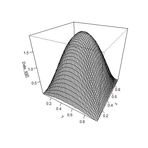
(a) $t=0.1$

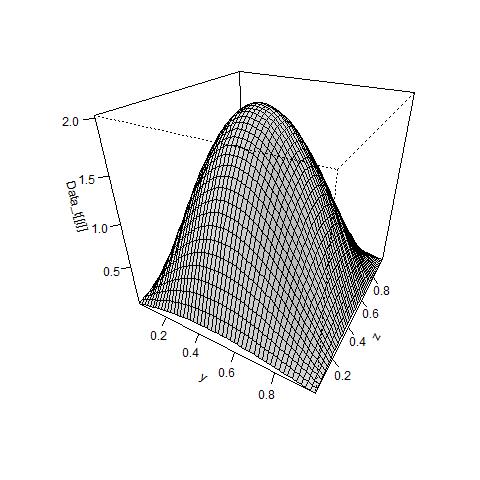
(b) $t=0.5$

(c) $t=0.9$

Figure 1. Cross sections of sample path with $\theta=(2,0.1,0.1,0.1)$, $\epsilon=0.01$ and $\lambda_{1,1}\approx 0$

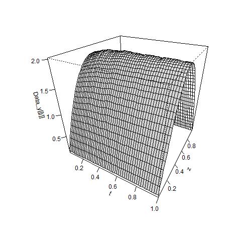
(a) $y=0.5$

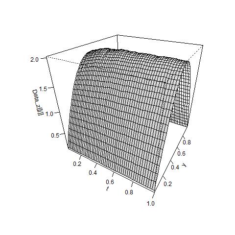
(b) $z=0.5$

Figure 2. Cross sections of sample path with $\theta=(2,0.1,0.1,0.1)$, $\epsilon=0.01$ and $\lambda_{1,1}\approx 0$

Figures 3-4 are the sample paths with $\theta=(4,0.3,0.3,0.3)$ and $\lambda_{1,1}\approx 2.07$. The cross section at $y=0.5$ in Figure 3-(A) corresponds to the cross section at $t=0.1$ in Figure 4-(A), and the cross section at $z=0.5$ in Figure 3-(A) corresponds to the cross section at $t=0.1$ in Figure 4-(B). For the case that $\lambda_{1,1}$ is positive, when $y$ and $z$ are fixed and $t$ tends to $1$, the value of $X^{Q_{1}}_{t}(y,z)$ approaches $0$. For example, when $y=z=0.5$, $X^{Q_{1}}_{0.1}(0.5,0.5)\approx 1.68$, $X^{Q_{1}}_{0.5}(0.5,0.5)\approx 0.74$, $X^{Q_{1}}_{0.9}(0.5,0.5)\approx 0.33$.

(a) $t=0.1$

(b) $t=0.5$

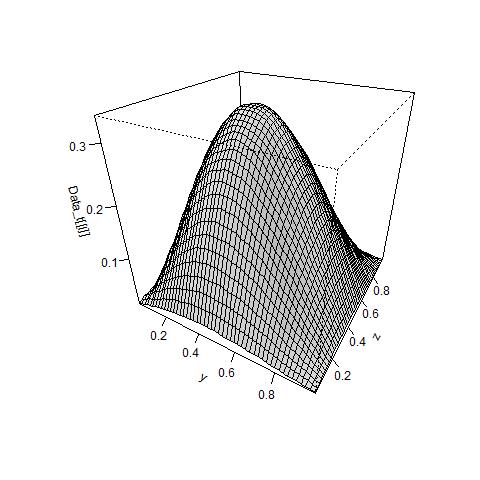
(c) $t=0.9$

Figure 3. Cross sections of sample path with $\theta=(4,0.3,0.3,0.3)$, $\epsilon=0.01$ and $\lambda_{1,1}\approx 2.07$

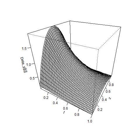
(a) $y=0.5$

(b) $z=0.5$

Figure 4. Cross sections of sample path with $\theta=(4,0.3,0.3,0.3)$, $\epsilon=0.01$ and $\lambda_{1,1}\approx 2.07$

Characteristic of $\epsilon$

Figures 5-7 show the sample paths with $\theta=(4,0.3,0.3,0.3)$ and the initial condition $\xi(y,z)=30y(1-y)z(1-z)$. $\theta_{0}$, $\theta_{1}$, $\eta_{1}$ and $\theta_{2}$ are fixed and only $\epsilon$ is changed. (A) in Figures 5-7 are cross sections with $\epsilon=0.01$. (B) in Figures 5-7 are cross sections with $\epsilon=0.25$. (C) in Figures 5-7 are cross sections with $\epsilon=0.5$. From Figures 5-7, it can be seen that the noise increases as $\epsilon$ increases.

(a) $\epsilon=0.01$

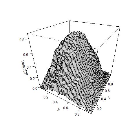
(b) $\epsilon=0.25$

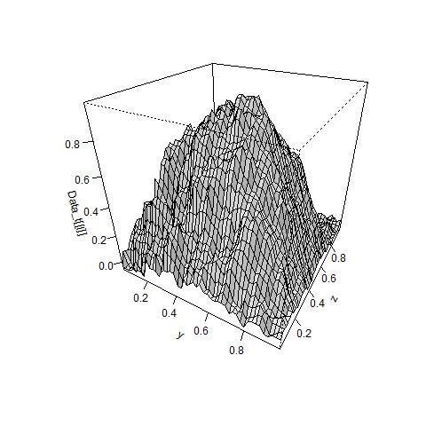
(c) $\epsilon=0.5$

Figure 5. Cross sections of sample path at $t=0.5$ with $\theta=(4,0.3,0.3,0.3)$ and $\lambda_{1,1}\approx 2.07$

(a) $\epsilon=0.01$

(b) $\epsilon=0.25$

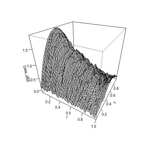
(c) $\epsilon=0.5$

Figure 6. Cross sections of sample path at $y=0.5$ with $\theta=(4,0.3,0.3,0.3)$ and $\lambda_{1,1}\approx 2.07$

(a) $\epsilon=0.01$

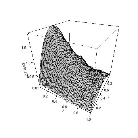
(b) $\epsilon=0.25$

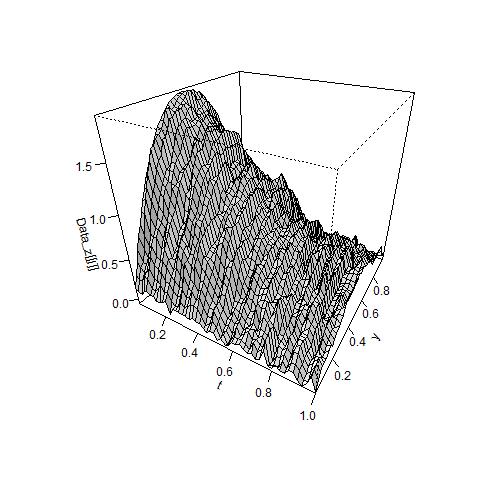
(c) $\epsilon=0.5$

Figure 7. Cross sections of sample path at $z=0.5$ with $\theta=(4,0.3,0.3,0.3)$ and $\lambda_{1,1}\approx 2.07$