A provably quasi-polynomial algorithm for the discrete logarithm problem in finite fields of small characteristic

Abstract

We describe a provably quasi-polynomial algorithm to compute discrete logarithms in the multiplicative groups of finite fields of small characteristic, that is finite fields whose characteristic is logarithmic in the order. We partially follow the heuristically quasi-polynomial algorithm presented by Barbulescu, Gaudry, Joux and Thomé. The main difference is to use a presentation of the finite field based on elliptic curves: the abundance of elliptic curves ensures the existence of such a presentation.

Keywords: discrete logarithm, finite fields, elliptic curves, quasi-polynomial, algebraic curves.

1 Introduction

A general formulation for the discrete logarithm problem is the following: given a group $G$, a generator $g\in G$ and another element $h\in G$, find an integer $z$ such that $g^{z}=h$. The hardness of this problem, which depends on the choice of $G$, is relevant for public-key cryptography since the very beginning of it [6].

We are concerned with the cases where $G$ is the multiplicative group of a finite field of small characteristic, which, for us, means a field of characteristic $p$ and cardinality $p^{n}$ for some integers $n>p$. Our main result is the following.

Theorem 1.1

There exists a probabilistic algorithm, described in Section 5, that solves the discrete logarithm problem in $K^{\times}$ for all finite fields $K$ of small characteristic in expected time

$$(\log\#K)^{O(\log\log\#K)}\,.$$

An algorithm with the above complexity is called quasi-polynomial.

The first heuristic quasi-polynomial algorithm solving the discrete logarithm in small characteristic was presented by Barbulescu, Gaudry, Joux and Thomé in [2]. One of their main ideas, originally in [9], is to look for a “simple” description of the Frobenius automorphism $\phi\colon K\to K$ and, if one can find such a simple description, to use it in an index calculus algorithm to find relations among the elements of the factor base more easily. In [8] was then presented another algorithm, based on similar ideas, whose expected complexity is proven to be quasi-polynomial when there exists “simple” description of the Frobenius automorphism (the notion of “simple” in [8] is slightly stricter than in [2]). In particular, we could deduce Theorem 1.1 if we knew that all finite fields of small characteristic $K$ can be embedded in a slightly larger field $K^{\prime}$ admitting a presentation as in [8]. The author is not aware of any proof of this fact, even though computations like [9, Table 1] support it and [17] gives a partial answer.

The author’s first incomplete attempt to prove Theorem 1.1 is his master’s thesis [16], which already contained the main idea of this article: using a different presentation for the finite field, stated in terms of the action of the Frobenius on an elliptic curve. Such “elliptic presentations” were first introduced in [5] and, since over a finite field $\mathbb{F}_{q}$ there are many non-isogenous elliptic curves, it is easy to prove that all finite fields of small characteristic can be embedded in a slightly larger field admitting such a presentation. The algorithm in [16] adapts the approach in [8] to finite fields with an elliptic presentations, but the proof of its correctness and quasi-polynomiality was not completed.

The idea of using elliptic presentations in this context has been independently developed by Kleinjung and Wesolowski, who have proved Theorem 1.1 in [14]. One of the differences between the present approach and the one in [14] is the proof of correctness and the quasi-polynomiality of the algorithms. In both cases it is a matter of showing the irreducibility of certain curves: the approach in [14] is to describe those curves as components of certain fibered products, as in [13], while we mostly rely on some Galois theory over function fields. Both approaches use some leght computations, which here are here mostly contained in Proposition 7.3 and in the Claims 9.2.3, 9.2.6, 9.3.2. A second difference between [14] and the present work is that in our algorithm the number of “traps” is finite and small, so that they can be included in the factor base, while in [14] there are infinitely many “traps” that need to be avoided by the algorithm.

In [10] Joux and Pierrot study a practical algorithm for the discrete logarithm based on elliptic presentations and apply it successfully in $\mathbb{F}_{3^{1345}}^{\times}$. Their experiments indicate that the efficiency of this algorithm is inferior, yet comparable, to the one in [11], the (heuristically) fastest currently known.

Structure of the paper

The structure of the article is as follows. In Section 2 we define elliptic presentations and we prove that all finite fields of small characteristic can be embedded in a slightly larger field admitting an elliptic presentation. Section 3 is about “traps” (cases that need different treatment in the algorithm). In Section 4 we describe the general setup of our algorithm and we explain how to pass from a factor base made of irreducible polynomials in $\mathbb{F}_{q}[x]$ to a factor base made of irreducible divisors on an elliptic curve $E/\mathbb{F}_{q}$. In Section 5 we give our algorithm, stated in terms of a descent procedure that is described in Section 6. A more precise statement about the complexity of the main algorithm is given in Theorem 5.4. Our descent procedure consists of two steps, presented and analysed in Section 6 under an assumption on certain varieties. These assumptions are proven in the subsequent sections: Section 7 gives a technical lemma, Section 8 proves the assumptions needed for the second and easier step and Section 9 proves the assumptions needed for the first step.

Acknowledgements

I thank René Schoof for introducing me to this research problem in $2016$ and for the useful ideas that lead to substantial simplifications of the proof.

The author is supported by the MIUR “Excellence Department Project MATH@TOV”, awarded to the Department of Mathematics, University of Rome, Tor Vergata, and by the “Programma Operativo (PON) “Ricerca e Innovazione” 2014-2020”

2 Elliptic presentations

One of the main ideas in [9] and in [2], is to present a field $K$ using two subfields $\mathbb{F}_{q}\subsetneq\mathbb{F}_{Q}\subseteq K$ of order $q,Q$ (both “small” compared to $\#K$) and an element $x_{1}\in K$ generating the extension $\mathbb{F}_{Q}\subset K$ such that the $q$-th Frobenius acts on $x_{1}$ in a simple way, namely $x_{1}^{q}=f(x_{1})$ for some $f\in\mathbb{F}_{q}(x)$ of degree at most $2$. We now define a presentation based on a similar idea: describing $K$ as $\mathbb{F}_{q}(x_{1},y_{1})$ where $\mathbb{F}_{q}$ is a finite field of order $q$ “small” compared to $\#K$ and $x_{1},y_{1}$ are two elements of $K$ on which the $q$-th Frobenius acts in a “simple” way.

Let $\mathbb{F}_{q}$ be a finite field of cardinality $q$, and let $K/\mathbb{F}_{q}$ be a field extension of of degree $n$. Suppose there exists an elliptic curve $E/\mathbb{F}_{q}$ defined by a Weierstrass equation and a point $P_{0}\in E(\mathbb{F}_{q})$ of order $n$. Denoting by $\phi$ be the $q$-th Frobenius on the elliptic curve $E$, the map $E\to E$ given by $P\mapsto\phi(P){-}P$ is surjective. Therefore there is a point $P_{1}=(x_{1},y_{1})$ on $E$ such that $\phi(P_{1})=P_{1}+P_{0}$. Hence

$(2.1)$ $$(x_{1}^{q^{i}},y_{1}^{q^{i}})=\phi^{i}(P_{1})=P_{1}+i\cdot P_{0}\quad\text{for every }i\in\mathbb{Z}\,,$$

implying that the field extension $\mathbb{F}_{q}\subset\mathbb{F}_{q}(x_{1},y_{1})$ has degree $n$. Hence $\mathbb{F}_{q}(x_{1},y_{1})$ is isomorphic to $K$. Moreover the $q$-th Frobenius acts on the pair $(x_{1},y_{1})$ in a “simple” way in the following sense: the addition formulas on $E$ give polynomials $f_{1},f_{2},f_{3}\in\mathbb{F}_{q}(x,y)$ of small degree such that $x_{1}^{q}=f_{1}(x_{1},y_{1})/f_{3}(x_{1},y_{1})$ and $y_{1}^{q}=f_{2}(x_{1},y_{1})/f_{3}(x_{1},y_{1})$. With this heuristic in mind, we give the following definition.

Definition 2.2

Let $E/\mathbb{F}_{q}$ be an elliptic curve defined by a Weierstrass polynomial in $\mathbb{F}_{q}[x,y]$, let $P_{0}$ be a $\mathbb{F}_{q}$-point on $E$ and let $\phi\colon E\to E$ be the $q$-th Frobenius. An $(E/\mathbb{F}_{q},P_{0})$-presentation of a finite field $K$ is an ideal $\mathfrak{M}\subset\mathbb{F}_{q}[x,y]$ such that

1. $K$ is isomorphic to $\mathbb{F}_{q}[x,y]/\mathfrak{M}$ with a chosen isomorphism;

2. there exists a point $P_{1}=(x_{1},y_{1})$ on $E$ such that $\mathfrak{M}=\{f\in\mathbb{F}_{q}[x,y]:f(x_{1},y_{1})=0\}$ and $\phi(P_{1})=P_{1}+P_{0}$;

3. $q>2$ and $[K:\mathbb{F}_{q}]>2$.

We sometimes omit the dependence on $(E/\mathbb{F}_{q},P_{0})$ and we simply write “elliptic presentation”. The hypothesis $q>2$ is used in the proof of Claim 9.2.3, while the hypothesis $[K:\mathbb{F}_{q}]>2$ is used in the following Remark, which is used in step $3$ of the main algorithm to lift elements of $K$ to polynomials in $\mathbb{F}_{q}[x]$, in particular to polynomials of degree a power of two.

Remark 2.3

If $\mathfrak{M}$ is an elliptic presentation, then the inclusion $\mathbb{F}_{q}[x]\to\mathbb{F}_{q}[x,y]$ induces an isomorphism $\mathbb{F}_{q}[x]/\mu\cong\mathbb{F}_{q}[x,y]/\mathfrak{M}$ for a certain $\mu\in\mathbb{F}_{q}[x]$.

Proving this is equivalent to proving that $x$ generates the extension $\mathbb{F}_{q}\subset\mathbb{F}_{q}[x,y]/\mathfrak{M}$. Using the notation in Definition 2.2, this is equivalent to proving that $\mathbb{F}_{q}(x_{1})$ is equal to $\mathbb{F}_{q}(x_{1},y_{1})$. If, for the sake of contradiction, this is not the case, then the Weierstrass equation satisfied by $x_{1}$ and $y_{1}$ implies that the extension $\mathbb{F}_{q}(x_{1})\subset\mathbb{F}_{q}(x_{1},y_{1})$ has degree $2$, hence $[\mathbb{F}_{q}(x_{1}):\mathbb{F}_{q}]=\tfrac{n}{2}$, where $n:=[\mathbb{F}_{q}(x_{1},y_{1}):\mathbb{F}_{q}]=[K:\mathbb{F}_{q}]$. Using Equation $(2.1)$, we deduce that

$$x(P_{1})=x_{1}=x_{1}^{q^{n/2}}=x(\phi^{n/2}P_{1})=x(P_{1}+\tfrac{n}{2}P_{0})\quad\implies\quad P_{1}+\tfrac{n}{2}P_{0}=\pm P_{1}\,.$$

Since, by Equation $(2.1)$, the order of $P_{0}$ is equal to $n$, we have $P_{1}+\tfrac{n}{2}P_{0}=-P_{1}$, implying that $2P_{1}$ lies $E(\mathbb{F}_{q})$. Therefore $P_{0}$ has order $2$, contradicting $n=[K:\mathbb{F}_{q}]>2$ in (iii).

We now show that any finite field $K$ of small characteristic can be embedded in a “slightly larger” field admitting an elliptic presentation with $q$ “small” compared to $\#K$.

Proposition 2.4

For any finite field $K$ of small characteristic there exists an extension $K\subset K^{\prime}$ having a elliptic presentation $\mathfrak{M}\subset\mathbb{F}_{q}[x,y]$ of $K^{\prime}$ such that

$$\log(\#K^{\prime})\leq 13\log(\#K)\log\log(\#K)\quad\text{and}\quad q\leq\log(\#K^{\prime})^{4}\,.$$

Moreover such $K^{\prime}$ and its presentation can be computed in polynomial time in $\log(\#K)$.

Proof.

Let $\#K=p^{n}$ for a prime $p$ and an integer $n>p$. Put $k_{0}:=\lceil\log_{p}n\rceil$ and $q:=p^{2k_{0}}$, so that $n$ has a multiple $n_{1}$ in the interval $[q-\sqrt{q}+1,q+1]$. If $n_{1}\equiv 1\bmod p$ we define $n_{2}:=n_{1}+n$, otherwise we define $n_{2}:=n_{1}$. Since $n_{2}$ in an integer contained in the Hasse interval $[q-2\sqrt{q}+1;q+2\sqrt{q}+1]$ that is not congruent to $1$ modulo $p$, by [19, Theorems 1a, 3] there exists an elliptic curve $E/\mathbb{F}_{q}$ whose group of rational points $E(\mathbb{F}_{q})$ is cyclic of order $n_{2}$. Since $n$ divides $n_{2}$, there exists a point $P_{0}\in E(\mathbb{F}_{q})$ of order $n$.

We can assume $E$ is defined by a Weierstrass polynomial. Since the map $P\mapsto\phi(P){-}P$ is surjective, there exists a point $(x_{1},y_{1})=P_{1}\in E(\overline{\mathbb{F}_{q}})$ such that $\phi(P_{1})=P_{1}+P_{0}$. Under the definition

$$\mathfrak{M}:=\{f\in\mathbb{F}_{q}[x,y]:f(x_{1},y_{1})=0\}\,,\quad K^{\prime}:=\mathbb{F}_{q}(x_{1},y_{1})\subset\overline{\mathbb{F}_{q}}\,,$$

it is clear that the map $\mathbb{F}_{q}[x,y]\to K$ sending $x\mapsto x_{1},y\mapsto y_{1}$ induces an isomorphism $\mathbb{F}_{q}[x,y]/\mathfrak{M}\cong K^{\prime}$. To prove that $\mathfrak{M}$ is an elliptic presentation of $K^{\prime}$, we are left to show that $q>2$ and $[K^{\prime}:\mathbb{F}_{q}]>2$: the first is is a consequence of the inequality $k_{0}=\lceil\log_{p}n\rceil>1$, the latter because, by ($(2.1)$), the degree of $\mathbb{F}_{q}\subset K^{\prime}$ is equal to the order $n$ of $P_{0}$, and $n>p\geq 2$.

Since $[K^{\prime}:\mathbb{F}_{q}]=n$ divides $[K^{\prime}:\mathbb{F}_{p}]$, the field $K^{\prime}$ has a subfield with $p^{n}$ elements. In other words $K$ can be embedded in $K^{\prime}$. Moreover we have

$$\log(\#K^{\prime})=n\log q<2n\log(p)(\log_{p}(n){+}1)\leq 4\log(p)\log(n)\leq 13\log(\#K)\log\log(\#K),$$

$$q=p^{2\lceil\log_{p}n\rceil}<p^{2+2\log_{p}n}=(pn)^{2}\leq n^{4}<\log(q^{n})^{4}=\log(\#K^{\prime})^{4}\,.$$

We now prove that it is possible to compute such $K^{\prime}$ and $\mathfrak{M}$ in polynomial time in $\log(\#K)$. We describe a procedure following the abstract part of the proof. Computing $k_{0},q,n_{1}$ is easy. We can construct a field $\mathbb{F}_{q}$ by testing the primality of all polynomials of degree $2k_{0}$ over $\mathbb{F}_{p}$ until an irreducible $\nu$ is found and define $\mathbb{F}_{q}=\mathbb{F}_{p}[T]/\nu$; since there are less than $n^{2}$ polynomials of this type, this takes polynomial time. Similarly we can find an elliptic curve $E$ with an $\mathbb{F}_{q}$-point $P_{0}$ of order $n$ in polynomial time, by listing all possible Weierstrass equations (there are less than $q^{6}$), testing if they define an elliptic curve and, when they do, enumerate all their $\mathbb{F}_{q}$-points. Then, using the addition formula on $E$, we write down the ideal $I\subset\mathbb{F}_{q}[x,y]$ whose vanishing locus inside $\mathbb{A}^{2}$ is the set of points $P=(x,y)\in E(\overline{\mathbb{F}_{q}})$ such that $\phi(P)=P+P_{0}$. As we showed before, the set of such points is non-empty, hence $I$ is a proper ideal and we can find a maximal ideal $\mathfrak{M}$ containing $I$. We don’t need general algorithms for primary decomposition since we can take $\mathfrak{M}=(\mu(x),\lambda(x,y))$, with $(\mu)$ being an irreducible factor of the generator of the ideal $J{\cap}\mathbb{F}_{q}[x]$ and $\lambda(x,y)$ being an irreducible factor of the image of the Weierstrass equation of $E$ inside $(\mathbb{F}_{q}[x]/\mu)[y]$. Since the Weiestrass polynomial is monic in $y$, we can assume that $\lambda$ is monic in $y$ too. Hence there is a point $P_{1}=(x_{1},y_{1})$ in the vanishing locus of $(\mu(x),\lambda(x,y))=\mathfrak{M}$. Since $\mathfrak{M}$ contains $I$, the point $P_{1}$ lies on $E$ and satisfies $\phi(P_{1})=P_{1}+P_{0}$. The maximality of $\mathfrak{M}$ implies that $\mathbb{F}_{q}[x,y](\mathfrak{M})=\mathbb{F}_{q}(x_{1},y_{1})=K^{\prime}$. Hence $\mathfrak{M}$ is the elliptic presentation we want. ∎

Notation.  For the rest of the article $\mathbb{F}_{q}$ is a finite field with $q$ elements, $\overline{\mathbb{F}_{q}}$ is its algebraic closure, $K$ is a finite extension of $\mathbb{F}_{q}$, the ideal $\mathfrak{M}\subset\mathbb{F}_{q}[x,y]$ is a $(E/\mathbb{F}_{q},P_{0})$-presentation of $K$, the map $\phi\colon E\to E$ is the $q$-th Frobenius and $P_{1}=(x_{1},y_{1})\in E(\overline{\mathbb{F}_{q}})$ is a point such that $\mathfrak{M}=\{f\in\mathbb{F}_{q}[x,y]:f(x_{1},y_{1})=0\}$. By $O_{E}$ we denote the neutral element of $E(\mathbb{F}_{q})$.

3 Traps

As first pointed out in [4], there are certain polynomials, called “traps” for which the descent procedure in [2] does not work. In [2] such traps are dealt with differently than the other polynomials. In [8] the notion of “trap” is extended: it includes not only polynomials for which the descent procedure is proven not to work, but also polynomials for which the strategy to prove the descent’s correctness does not work. In [8] traps are avoided by the algorithm.

In the following sections we describe a descent procedure stated in terms of points and divisors on $E$ and there are certain points in $E(\overline{\mathbb{F}_{q}})$ that play the role of “traps”, as in [8]. The definition of this subset of $E(\overline{\mathbb{F}_{q}})$ is rather cumbersome, but it is easy to deduce that we have less than $15q^{4}$ traps. In particular, in contrast to [8], we can include them in the factor base without enlarging it too much.

Definition 3.1

A point $P\in E(\overline{\mathbb{F}_{q}})$ is a trap if it satisfies one of the following conditions:

$$2P=0\,,\quad\text{ or }\quad(2\phi-\mathrm{Id})(\phi^{2}-\phi+\mathrm{Id})(P)=P_{0}\,,\quad\text{ or }\quad(2\phi-\mathrm{Id})(\phi+\mathrm{Id})(P)=2P_{0}$$

$$\text{or }(\phi^{4}-\mathrm{Id})(P)=4P_{0}\,,\quad\text{ or }2(\phi^{3}-\mathrm{Id})(P)=6P_{0}\,,\quad\text{ or }\quad(2\phi+\mathrm{Id})(\phi-\mathrm{Id})(P)=2P_{0}\,.$$

In ($(\mathrm{8.2.2})$) and at the beginning of the proof of Claim 9.2.3 we explain why these points interfere with our strategy of proof.

4 Divisors and discrete logarithm

We recall that the Galois group of $\mathbb{F}_{q}$ acts on the group of divisors on $E$ by the formula

$$\sigma\left(\sum_{P\in E(\overline{\mathbb{F}_{q}})}n_{P}P\right)=\sum_{P\in E(\overline{\mathbb{F}_{q}})}n_{P}\,\sigma(P)\,.$$

For any algebraic extension $\mathbb{F}_{q}\subset k$ we denote $\mathrm{Div}_{k}(E)$ the the set of divisors defined over $k$, namely the divisors $D$ such that $\sigma D=D$ for all $\sigma\in\mathrm{Gal}(\overline{\mathbb{F}_{q}}/k)$. We say that a divisor is irreducible over $k$ if it is the sum, with multiplicity $1$, of all the $\mathrm{Gal}(\overline{\mathbb{F}_{q}}/k)$-conjugates of some point $P\in E(\overline{\mathbb{F}_{q}})$. Every divisor defined over $k$ is a $\mathbb{Z}$-combination of irreducible divisors over $k$. We refer to [20, Chapter $2$] for the definitions of principal divisor and support of a divisor.

We need two quantities to describe the “complexity” of a divisor. The first one is the absolute degree of a divisor, defined as as

$$\mathrm{absdeg}\left(\sum_{P\in E(\overline{\mathbb{F}_{q}})}n_{P}(P)\right):=\sum_{P\in E(\overline{\mathbb{F}_{q}})}|n_{P}|\,.$$

The second quantity is analogous to the degree of the splitting field of a polynomial, but we decide to “ignore” trap points. Given a divisor $D\in\mathrm{Div}_{k}(E)$, we denote $D^{\mathrm{noTrap}}$ the part of $D$ that is supported outside the set of trap points, which is also defined over $k$ because the set of trap points is $\mathrm{Gal}(\overline{\mathbb{F}_{q}}/\mathbb{F}_{q})$-invariant. We define the essential degree of $D$ over $k$ to be the least common multiple of the degrees of the irreducible divisors appearing in $D^{\mathrm{noTrap}}$. In other words, if we denote as $k(D^{\mathrm{noTrap}})$ the minimal algebraic extension $\widetilde{k}\supset k$ such that the support of $D$ is contained in $E(\widetilde{k})$, then

$$\mathrm{essdeg}_{k}(D):=[k(D^{\mathrm{noTrap}}):k]\,.$$

If $D^{\mathrm{noTrap}}=0$ we take $\mathrm{essdeg}_{k}(D)=1$.

Now consider the discrete logarithm problem in a field having an elliptic presentation $\mathfrak{M}$. First of all, if $q$ is small compared to $\#K$, for example $q\leq(\log K)^{4}$ as in Proposition 2.4, and if we are able to compute discrete logarithms in $K^{\times}/\mathbb{F}_{q}^{\times}$ in quasi-polynomial time, then we can also compute discrete logarithms in $K^{\times}$ in quasi-polynomial time. Hence in the rest of the article we are concerned with computing discrete logarithms in $K^{\times}/\mathbb{F}_{q}^{\times}$.

Denoting $\mathbb{F}_{q}[x,y]_{\mathfrak{M}}$ the localization of $\mathbb{F}_{q}[x,y]$ at the maximal ideal $\mathfrak{M}$, we have

$$K\,\cong\,\mathbb{F}_{q}[x,y]/\mathfrak{M}\,\cong\,\mathbb{F}_{q}[x,y]_{\mathfrak{M}}/\mathfrak{M}_{\mathfrak{M}}\,.$$

An element $f$ of $(\mathbb{F}_{q}[x,y]_{\mathfrak{M}})^{\times}$ defines a rational function on $E$ which is defined over $\mathbb{F}_{q}$ and regular and non-vanishing in $P_{1}$. We represent elements in $K^{\times}/\mathbb{F}_{q}^{\times}$ with elements of $\mathbb{F}_{q}(E)$ that are regular and non-vanishing on $P_{1}$.

Let $g,h$ be elements of $\mathbb{F}_{q}(E)$ both regular and non-vanishing on $P_{1}$ and let us suppose that $g$ generates the group $K^{\times}/\mathbb{F}_{q}^{\times}$. Then the logarithm of $h$ in base $g$ is a well defined integer modulo $\tfrac{\#K{-}1}{q{-}1}$ that we denote $\log_{\mathfrak{M},g}(h)$ or simply $\log h$. Since we are working modulo $\mathbb{F}_{q}^{\times}$, the logarithm of $h$ only depends on the divisor of zeroes and poles of $h$: if $h^{\prime}\in\mathbb{F}_{q}(E)$ satisfies $\mathrm{div}(h)=\mathrm{div}(h^{\prime})$, then $h/h^{\prime}\in\mathbb{F}_{q}^{\times}$ and consequently $\log(h)=\log(h^{\prime})$. Hence, putting

$$\log(\mathrm{div}(h)):=\log(h)\,,$$

we define the discrete logarithm as homomorphism whose domain is the subgroup of $\mathrm{Div}_{\mathbb{F}_{q}}(E)$ made of principal divisors, supported outside $P_{1}$ and whose image is $\mathbb{Z}/(\tfrac{\#K{-}1}{q{-}1})\mathbb{Z}$. The kernel of this morphism is a subgroup of $\mathrm{Div}_{\mathbb{F}_{q}}(E)$, hence it defines the following equivalence relation on $\mathrm{Div}_{\mathbb{F}_{q}}(E)$

$(4.1)$ $\displaystyle D_{1}\sim D_{2}$ $\displaystyle\iff D_{1}-D_{2}\in\mathrm{Ker}(\log)$

$$\iff\exists f\in\mathbb{F}_{q}(E)\mbox{ such that }f(P_{1})=1\mbox{ and }\mathrm{div}(f)=D_{1}-D_{2}\,.$$

We notice that this equivalence relation does not depend on $g$ and that, given rational functions $h_{1},h_{2}\in\mathbb{F}_{q}(E)$ regular and non-vanishing on $P_{1}$, we have $\log h_{1}=\log h_{2}$ if and only if $\mathrm{div}(h_{1})\sim\mathrm{div}(h_{2})$. Motivated by this, for all divisors $D_{1},D_{2}\in\mathrm{Div}_{\mathbb{F}_{q}}(E)$ we use the notation

$$\log_{\mathfrak{M}}D_{1}=\log_{\mathfrak{M}}D_{2}\iff D_{1}\sim D_{2}\,.$$

Notice that we do not define the expression $\log_{\mathfrak{M}}(D)$ or $\log_{\mathfrak{M},g}(D)$ for any $D$ in $\mathrm{Div}_{\mathbb{F}_{q}}(E)$, since the function $\log$ might not extend to a morphism $\mathrm{Div}_{\mathbb{F}_{q}}(E)\to\mathbb{Z}/(\tfrac{\#K{-}1}{q{-}1})\mathbb{Z}$. In our algorithm we use the equivalence relation ($(4.1)$) to recover equalities of the form $\log h_{1}=\log h_{2}$.

5 The main algorithm

As in [8] our algorithm is based on a descent procedure, stated in terms of divisors on $E$.

Theorem 5.1

There exists an algorithm, described in the proof, that takes as input an $(E/\mathbb{F}_{q},P_{0})$-presentation $\mathfrak{M}$ and a divisor $D\in\mathrm{Div}_{\mathbb{F}_{q}}(E)$ such that $\mathrm{essdeg}_{\mathbb{F}_{q}}(D)=2^{m}$ for some integer $m\geq 7$ and computes a divisor $D^{\prime}\in\mathrm{Div}_{\mathbb{F}_{q}}(E)$ such that

$$\log_{\mathfrak{M}}D=\log_{\mathfrak{M}}D^{\prime}\,,\quad(\mathrm{essdeg}_{\mathbb{F}_{q}}D^{\prime})\mid 2^{m-1}\,,\quad\mathrm{absdeg}(D^{\prime})\leq 4q^{2}\mathrm{absdeg}D\,.$$

This algorithm is probabilistic and runs in expected polynomial time in $q\mathrm{absdeg}(D)$.

Applying repeatedly the algorithm of the above theorem we deduce the following result.

Corollary 5.2

There exists an algorithm, described in the proof, that takes as input an $(E/\mathbb{F}_{q},P_{0})$-presentation and a divisor $D\in\mathrm{Div}_{\mathbb{F}_{q}}(E)$ such that $\mathrm{essdeg}_{\mathbb{F}_{q}}D=2^{m}$ for some integer $m$ and computes a divisor $D^{\prime}\in\mathrm{Div}_{\mathbb{F}_{q}}(E)$ such that

$$\log_{\mathfrak{M}}D=\log_{\mathfrak{M}}D^{\prime}\,,\quad\mathrm{essdeg}_{\mathbb{F}_{q}}D^{\prime}\mid 64\,,\quad\mathrm{absdeg}(D^{\prime})\leq(2q)^{2m}\mathrm{absdeg}(D)\,.$$

This algorithm is probabilistic and runs in expected polynomial time in $q^{m}\mathrm{absdeg}(D)$.

The algorithm in [8] is based on the descent procedure [8, Theorem 3]. Using the same ideas we use the descent procedure of the last corollary to describe our main algorithm, which computes discrete logarithms in finite fields with an elliptic presentation.

The idea is setting up an index calculus with factor base the irreducible divisors whose essential degree divides $64$. To collect relations we use a “zig-zag descent”: for every $f=g^{a}h^{b}$, we first use the polynomial $\mu$ determined in Remark 2.3 to find $f^{\prime}\equiv f\bmod\mathfrak{M}$ such that the essential degree of $\mathrm{div}(f^{\prime})$ is a power of $2$, and we then apply the descent procedure to express $\log(f)=\log(f^{\prime})$ as the logarithm of sums of elements in the factor base.

Main Algorithm

Input: an $(E/\mathbb{F}_{q},P_{0})$-epresentation $\mathfrak{M}\subset\mathbb{F}_{q}[x,y]$ of a field $K$ and two polynomials $g,h\in\mathbb{F}_{q}[x,y]\setminus\mathfrak{M}$ such that $g$ generates the group $\left(\mathbb{F}_{q}[x,y]/\mathfrak{M}\right)^{\times}/\mathbb{F}_{q}^{\times}$.

Output: an integer $z$ such that

$$g^{z}\equiv\gamma\cdot h\pmod{\mathfrak{M}}\quad\mbox{ for some }\gamma\in\mathbb{F}_{q}^{\times}\,,$$

which is equivalent to $g^{z}=h$ in the group $K^{\times}/\mathbb{F}_{q}^{\times}$.

1. Preparation: Compute the monic polynomial $\mu\in\mathbb{F}_{q}[x]$ generating the ideal $\mathfrak{M}\cap\mathbb{F}_{q}[x]$. Compute polynomials $\tilde{g},\tilde{h}\in\mathbb{F}_{q}[x]$ such that $\tilde{g}\equiv g$ and $\tilde{h}\equiv h$ modulo $\mathfrak{M}$. Put $c:=\#E(\mathbb{F}_{q})$, $n:=\deg\mu$ and $m:=\lceil\log n\rceil+3$.

2. Factor base: List the irreducible divisors $D_{1},\ldots,D_{t}\in\mathrm{Div}_{\mathbb{F}_{q}}(E)$ that do not contain $P_{1}$ and either have degree dividing $64$ or are supported on the trap points.

3. Collecting relations: For $j=1,\ldots,t{+}1$ do the following:

   Pick random integers $\alpha_{j},\beta_{j}\in\{1,\ldots,\tfrac{q^{n}-1}{q-1}\}$ and compute $\tilde{g}^{\alpha_{j}}\tilde{h}^{\beta_{j}}$. Pick random polynomials $f(x)$ of degree $2^{m}$ such that $f\equiv\tilde{g}^{\alpha_{j}}\tilde{h}^{\beta_{j}}\pmod{\mu}$ until $f$ is irreducible. Apply the descent procedure in Corollary 5.2 to find $v_{j}=(v_{j,1},\ldots,v_{j,t})\in\mathbb{Z}^{t}$ such that

   $$\log_{\mathfrak{M}}\left(\mathrm{div}(f)\right)=\log_{\mathfrak{M}}\left(v_{j,1}D_{1}+\ldots+v_{j,t}D_{t}\right)\,.$$

4. Linear algebra: Compute $d_{1},\ldots,d_{t+1}\in\mathbb{Z}$ such that $\gcd(d_{1},\ldots,d_{t+1})=1$ and

   $$d_{1}v_{1}+\ldots+d_{t+1}v_{t+1}\equiv(0,\ldots,0)\pmod{\tfrac{q^{n}-1}{q-1}c}\,.$$

   Put $a:=d_{1}\alpha_{1}+\ldots+d_{t+1}\alpha_{t+1}$ and $b:=d_{1}\beta_{1}+\ldots+d_{t+1}\beta_{t+1}$.

5. Finished?: If $b$ is not invertible modulo $\tfrac{q^{n}-1}{q-1}$ go back to step $3$, otherwise output

   $$z:=-ab^{-1}\,\left(\bmod{\,\tfrac{q^{n}-1}{q-1}}\right)$$

Analysis of the main algorithm

We first prove, assuming Theorem 5.1, that the algorithm, when it terminates, gives correct output. First of all we notice that, as explained in Remark 2.3, the polynomials $\mu,\tilde{g}$ and $\tilde{h}$ exist and that $\tilde{g}$ and $\tilde{h}$ define the same element as $g$, respectively $h$, in $K\cong\mathbb{F}_{q}[x,y]/\mathfrak{M}$. Let $d_{j},\alpha_{j},\beta_{j}$ and $v_{j}$ be the integers and vectors of integers stored at the beginning of the fourth step the last time it is executed. By definition of $d_{j}$, we have

$$\sum_{j=1}^{t+1}\sum_{i=1}^{t}d_{j}v_{j,i}D_{i}=\tfrac{q^{n}-1}{q-1}c\cdot D\,,$$

for a certain $D\in\mathrm{Div}_{\mathbb{F}_{q}}(E)$. The divisor $cD$ is principal because $c=\#\mathrm{Pic}^{0}(E/\mathbb{F}_{q})$ and, since for all $j$ the divisor $\sum_{i}v_{j,i}D_{i}$ is principal, $D$ has degree $0$. Choosing $\lambda$ in $\mathbb{F}_{q}(E)$ such that $\mathrm{div}(\lambda)=cD$, we have

$(5.3)$ $$\sum_{j=1}^{t+1}\sum_{i=1}^{t}d_{j}v_{j,i}D_{i}=\mathrm{div}(\lambda^{\frac{q^{n}-1}{q-1}})\,.$$

Writing $\log$ for $\log_{\mathfrak{M},g}$, by definition of $v_{j}$ we have

$$\log(g^{\alpha_{j}}h^{\beta_{j}})=\log\left(\sum_{i=1}^{t}v_{j,i}D_{i}\right)\,.$$

This, together with Equation ($(5.3)$), imply the following equalities in $\mathbb{Z}/\tfrac{q^{n}-1}{q-1}\mathbb{Z}$

$$a+b\log(h) =\sum_{j=1}^{t+1}d_{j}(\alpha_{j}+\beta_{j}\log(h))=\sum_{j=1}^{t+1}d_{j}\log(g^{\alpha_{j}}h^{\beta_{j}})=\sum_{j=1}^{t+1}d_{j}\log\left(\sum_{i=1}^{t}v_{j,i}D_{i}\right)$$

$$=\log\left(\sum_{j=1}^{t+1}\sum_{i=1}^{t}d_{j}v_{j,i}D_{i}\right)=\log\left(\mathrm{div}(\lambda^{\frac{q^{n}-1}{q-1}})\right)=\tfrac{q^{n}-1}{q-1}\log(\lambda)=0\,,$$

implying that the output $z$ of the algorithm is correct.

We now estimate the running time step by step. The first step can be performed with easy Groebner basis computations. Now the second step. We represent irreducible divisors $D$ not supported on $O_{E}$ in the following way: either $D$ is the vanishing locus of a prime ideal $(a(x),W(x,y))$ with $a$ monic and irreducible and $W$ the Weierstrass polynomial defining $E$, or $D$ is the vanishing locus of a prime ideal $(a(x),y-b(x))$ for some polynomials $a,b\in\mathbb{F}_{q}[x]$ and $a$ monic irreducible; in the first case $\deg D=2\deg a$, in the second case $\deg D=\deg a$. We can list all the irreducible divisors with degree dividing $64$ by listing all monic irreducible polynomials $\mu_{1},\ldots,\mu_{r}\in\mathbb{F}_{q}[x]$ of degree dividing $64$ and, for each $i$ compute the prime ideals containing $(\mu_{i},W)$, which amounts to factoring $W$ as a polynomial in $y$, considered over the field $\mathbb{F}_{q}[x]/\mu_{i}$. Listing all the divisors supported on the trap points can be done case by case. For example we can list the irreducible divisors supported on the set $S:=\{P\in E(\overline{\mathbb{F}_{q}}):\phi^{4}(P)-P=4P_{0}\}$ by writing down, with the addition formula on $E$, an ideal $J\subset\mathbb{F}_{q}[x,y]$ whose vanishing locus is $S\subset\mathbb{A}^{2}(\overline{\mathbb{F}}_{q})$ and computing all the prime ideals containing $J$. The divisor $O_{E}$ appears among $D_{1},\ldots,D_{s}$ because $O_{E}$ is a trap point. Since there are $q^{64}$ monic polynomials of degree $64$ and at most $15q^{4}$ trap points and since, using [1], factoring a polynomial of degree $d$ in $\mathbb{F}_{q}[x]$ takes on average $O(\log(q)d^{3})$ operations, the second step takes polynomial time in $q$. Moreover, we have $t\leq 2q^{64}$.

Now the third step. By [21, Theorem 5.1], if $f(x)$ is a random polynomial of degree $2^{m}$ congruent to $\tilde{g}^{\alpha_{j}}\tilde{h}^{\beta_{j}}$ modulo $\mu$, then the probability of $f$ being irreducible is at least $2^{-m-1}$. Therefore finding a good $f$ requires on average $O(2^{m})=O(n)$ primality tests, hence $O(n^{4}\log q)$ operations. By assumption finding the vector $v_{j}$ requires polynomial time in $q^{m}2^{m+1}$. We deduce that the third step has probabilistic complexity $tq^{O(\log n)}=q^{O(\log n)}$.

The fourth step can be can be performed by computing a Hermite normal form of the matrix having the $v_{j}$’s as columns. Since $c\leq q{+}2\sqrt{q}+1$, the entries of the $v_{j}$ are at most as big as $4q^{n+1}$. Therefore the fourth step is polynomial in $t\log(q^{n})$, hence polynomial in $n$.

The last step only requires arithmetic modulo $(q^{n}{-}1)/(q{-}1)$.

To understand how many times each step is repeated on average, we need to estimate the probability that, in the last step, $b$ is invertible modulo $(q^{n}{-}1)/(q{-}1)$ and to do so we look at the quantities in the algorithms as if they were random variables. The vector $(d_{1},\ldots,d_{t+1})$ only depends on the elements $h^{\alpha_{j}}g^{\beta_{j}}$’s and on the randomness contained in the descent procedure and in step $2$. Since the $\alpha_{j}$’s and $\beta_{j}$’s are independent variables and since $g$ is a generator, we deduce that the vector $(\beta_{1},\ldots,\beta_{t+1})$ is independent of $(g^{\alpha_{1}}h^{\beta_{1}},\ldots,g^{\alpha_{t+1}}h^{\beta_{t*1}})$, hence also independent of the vector $(d_{1},\ldots,d_{t+1})$. Since $(\beta_{1},\ldots,\beta_{t+1})$ takes on all values in $\{0,\ldots,q^{n}-1\}^{t+1}$ with the same probability and $\mathrm{gcd}(d_{1},\ldots,d_{t+1})=1$, then

$$b=d_{1}\beta_{1}+\ldots d_{t+1}\beta_{t+1}$$

takes all values in $\mathbb{Z}/(q^{n}-1)\mathbb{Z}$ with the same probability. Hence

$$\Big{(}\text{probability that $b$ is coprime to }\tfrac{q^{n}-1}{q-1}\Big{)}=\phi\left(\tfrac{q^{n}-1}{q-1}\right)/\tfrac{q^{n}-1}{q-1}\gg\frac{1}{\log\log q^{n}}$$

When running the algorithm, the first and the second step get executed once and the other steps get executed the same number of times, say $r$, whose expected value is the inverse of the above probability. Since $r$ is $O(\log\log(q^{n}))$ on average and each step has average complexity at most $q^{O(\log n)}$, the average complexity of the algorithm is $O(q^{O(\log n)})$. Hence, assuming Theorem 5.1 we have proved the following theorem.

Theorem 5.4

The above Main Algorithm solves the discrete logarithm problem in the group $K^{\times}/\mathbb{F}_{q}^{\times}$ for all finite fields $K$ having an elliptic presentation $\mathfrak{M}\subset\mathbb{F}_{q}[x,y]$. It runs in expected time $q^{O(\log[K:\mathbb{F}_{q}])}$.

Theorem 1.1 follows from Theorem 5.4 and Proposition 2.4: the latter states that any finite field of small characteristic $K$ can be embedded in a slightly larger field $K^{\prime}$ having an elliptic presentation $\mathfrak{M}\subset\mathbb{F}_{q}[x,y]$ such that $q\leq\log(\#K^{\prime})^{4}$ and Theorem 1.1 implies that the discrete logarithm problem is at most quasi-polynomial for such a $K^{\prime}$. Moreover, by Proposition 2.4, such a $K^{\prime}$, together with its elliptic presentation, can be found in polynomial time in $\log(\#K)$, by [15] we can compute an embedding $K\hookrightarrow K^{\prime}$ in polynomial time in $\log(\#K)$ and by [18, Theorem $15$] a random element $g^{\prime}\in K^{\prime}$ has probability $\phi(\#K^{\prime})/\#K^{\prime}\gg 1/\log\log\#K^{\prime}$ of being a generator of $K^{\prime}$: hence, given elements $g,h\in K$, we can compute $\log_{g}(h)$ by embedding $K$ inside $K^{\prime}$ and trying to compute the pair $(\log_{g^{\prime}}g,\log_{g^{\prime}}h)$ for different random values of $g^{\prime}\in K^{\prime}$.

Proposition 2.4 is proven, while Theorem 5.4 relies on the the existence of a descent procedure as described in Theorem 5.1. In the rest of the article, we describe this descent procedure.

6 The descent procedure

In this chapter we describe the descent procedure of Theorem 5.1. To do so, we do a couple of reductions, we split the descent in two steps and, in both steps, we reduce our problem to the computation of $k$-rational points on certain varieties for a certain extension $k$ of $\mathbb{F}_{q}$. In Sections 7, 8, 9 we give the exact definition of these varieties and we prove that they have many $k$-rational points, which implies that our algorithm has a complexity as in Theorem 5.1.

Let $D$ be as in Theorem 5.1. If $D$ is supported on the set of trap points, we can gust pick $D^{\prime}=D$, hence we can suppose that $D$ is supported outside the traps. Moreover, we can write $D$ as a combination of divisors $D_{i}$ that are irreducible over $\mathbb{F}_{q}$, apply the descent to the $D_{i}$’s and take a linear combination of the results to reconstruct a possible $D^{\prime}$. Hence, we can suppose that $D$ is irreducible over $\mathbb{F}_{q}$, that is, if we write $2^{m}=4l$, we can suppose that

$$D=Q+\sigma Q+\ldots+\sigma^{4l-1}Q\,,$$

for $Q$ a non-trap point on $E$ such that $[\mathbb{F}_{q}(Q):\mathbb{F}_{q}]=4l=2^{m}$ and $\sigma$ a generator of $\mathrm{Gal}(\mathbb{F}_{q}(Q)/\mathbb{F}_{q})$.

We can do a sort of “base change to $k$”. Let $k$ be the unique subfield of $\mathbb{F}_{q}(Q)$ such that $[k:\mathbb{F}_{q}]=l$ and let us define

$$\tilde{D}:=Q+\sigma^{l}Q+\sigma^{2l}Q+\sigma^{3l}Q\quad\in\mathrm{Div}_{k}(E)\,.$$

If we are able to find a divisor $\tilde{D}^{\prime}\in\mathrm{Div}_{k}(E)$ and a rational function $g\in k(E)$ such that

$(6.1)$ $\displaystyle\qquad\mathrm{absdeg}\tilde{D}^{\prime}\leq 16q^{2}\,,\qquad\qquad\mathrm{essdeg}_{k}\tilde{D}^{\prime}\mid 2$

$$\mathrm{div}(g)=\tilde{D}-\tilde{D}^{\prime}\,,\qquad\qquad g(\tau(P_{1}))=1\quad\mbox{for all }\tau\in\mathrm{Gal}(\overline{\mathbb{F}_{q}}/\mathbb{F}_{q})\,,\,,$$

then the divisor

$$D^{\prime}:=\tilde{D}^{\prime}+\sigma(\tilde{D}^{\prime})+\ldots\sigma^{l-1}(\tilde{D}^{\prime})\,,$$

satisfies the conditions in Theorem 5.1: the absolute and essential degree of $D^{\prime}$ are easy to estimate and we have $\log_{\mathfrak{M}}D=\log_{\mathfrak{M}}D^{\prime}$ because the rational function $f:=gg^{\sigma}\cdots g^{\sigma^{l-1}}$ satisfies $f(P_{1})=1$ and $\mathrm{div}(f)=D-D^{\prime}$.

Hence, in order to prove Theorem 5.1, it is enough to describe a probabilistic algorithm that takes $k$ and $\tilde{D}$ as input and, in expected polynomial time in $ql$, computes $g,\tilde{D}^{\prime}$ as in $(6.1)$. Such an algorithm can be obtained by applying in sequence the algorithms given by the following two propositions. In other words, the descent procedure is split in two steps.

Proposition 6.2

There is an algorithm, described in the proof, with the following properties

• it takes as input an $(E/\mathbb{F}_{q},P_{0})$-presentation, a finite extension $\mathbb{F}_{q}\subset k$ of degree at least $80$ and a divisor $D\in\mathrm{Div}_{k}(E)$ such that $\mathrm{essdeg}_{k}D=4$

• it computes a rational function $g\in k(E)$ and a divisor $D^{\prime}=D_{1}+D_{2}\in\mathrm{Div}_{k}(E)$ such that

  $$D-D^{\prime}=\mathrm{div}(g)\,,\quad g(P)=1\,\,\mbox{for all }P\in E(\overline{\mathbb{F}_{q}})\mbox{ such that }\phi(P)=P+P_{0}\,,$$

  $$\mathrm{essdeg}_{k}(D_{1})\mid 3\,,\quad\mathrm{essdeg}_{k}(D_{2})\mid 2\,,\quad\mathrm{absdeg}D_{1}+\mathrm{absdeg}D_{2}\leq 2q\mathrm{absdeg}D\,;$$

• it is probabilistic and runs in expected polynomial time in $q{\cdot}\log(\#k){\cdot}\mathrm{absdeg}(D)$.

Proposition 6.3

There is an algorithm, described in the proof, with the following properties

• it takes as input an $(E/\mathbb{F}_{q},P_{0})$-presentation, an extension of finite fields $\mathbb{F}_{q}\subset k$ of degree at least $80$ and a divisor $D\in\mathrm{Div}_{k}(E)$ such that $\mathrm{essdeg}_{k}D=3$;

• it computes a rational function $g\in k(E)$ and a divisor $D^{\prime}\in\mathrm{Div}_{k}(E)$ such that

  $$D-D^{\prime}=\mathrm{div}(g)\,,\quad g(P)=1\,\,\mbox{for all }P\in E(\overline{\mathbb{F}_{q}})\mbox{ such that }\phi(P)=P+P_{0}\,,$$

  $$\quad\mathrm{essdeg}_{k}(D^{\prime})\mid 2\,,\quad\mathrm{absdeg}(D^{\prime})\leq 2q\mathrm{absdeg}(D)\,;$$

• it is probabilistic and runs in expected polynomial time in $q{\cdot}\log(\#k){\cdot}\mathrm{absdeg}(D)$.

We now describe our strategy of proof for the above propositions. Let $\varepsilon:=\mathrm{essdeg}_{k}(D)$ (hence $\varepsilon=3$ for Proposition 6.3 and $\varepsilon=4$ for Proposition 6.2). Again, $D$ can be supposed to be irreducible over $k$ and supported outside the traps, i.e.

$$D=Q+\ldots+\sigma^{\varepsilon-1}Q\,,$$

for $Q$ a non-trap point on $E$ such that $[k(Q):k]=\varepsilon$, and $\sigma$ a generator of $\mathrm{Gal}(k(Q)/k)$.

Let $\tau_{P_{0}}$ be the translation by $P_{0}$ on $E$ and let $h\mapsto h^{\phi}$ be the automorphism of $k(E)$ that “applies $\phi$ to the coefficients of $h$” (denoting $x,y$ be the usual coordinates on $E$, we have $x^{\phi}=x$, $y^{\phi}=y$ and $\alpha^{\phi}=\alpha^{q}$ for all $\alpha\in k$). Using this notation, we rephrase one of Joux’s ideas ([9]) in the following way: for every point $P\in E(\overline{\mathbb{F}_{q}})$ such that $\phi(P)=P+P_{0}$ and for every function $f\in k(E)$ regular on $P$ we have

$(6.4)$ $$f(P)^{q}=f^{\phi}(\phi(P))=f^{\phi}(P+P_{0})=(f^{\phi}\circ\tau_{P_{0}})(P)\,,$$

hence, for all $a,b,c,d\in k$ such that $cf^{q+1}{+}df^{q}{+}af{+}b$ does not vanish on $P$, the rational function

$(6.5)$ $$g:=\frac{(cf+d)(f^{\phi}\circ\tau_{P_{0}})+af+b}{cf^{q+1}+df^{q}+af+b}\,,$$

satisfies

$$g(P)=1\quad P\in E(\overline{\mathbb{F}_{q}}) \phi(P)=P+P_{0}$$ for all such that .

Hence, for a function $g$ as in ($(6.5)$), one of the requirements of Propositions 6.2 (respectively 6.3) is automatically satisfied. In the algorithm we look for a function $g$ of that form. We now look for conditions on $f$ and $a,b,c,d$ implying that the function $g$ and the divisor

$(6.6)$ $$D^{\prime}:=D-\mathrm{div}(g)\,,$$

have the desired properties.

One of these properties is “$\mathrm{essdeg}_{k}(D^{\prime})\leq\varepsilon-1$”. for which it is enough that “$[k(P):k]\leq\varepsilon-1$ for all the points $P$ in the support of $D$”. In particular the support of $D^{\prime}$ contains all the poles of $g$, which are either poles of $f$, poles of $f^{\phi}\circ\tau_{P_{0}}$ or zeroes of $cf^{q+1}{+}df^{q}{+}af{+}b$. Since the zeroes and poles of a function $h\in k(E)$ are defined over an extension of $k$ of degree at most $\deg(h)$, the following conditions are sufficient to take care of the poles of $g$:

1. the function $f$ has at most $\varepsilon{-}1$ poles counted with multiplicity;

2. the polynomial $cT^{q+1}+dT^{q}+aT+b$ splits into linear factors in $k[T]$.

Here we are using another idea from [9], namely that, if $f$ has low degree (i.e. few poles), then the numerator of ($(6.5)$) has low degree too, and the denominator has a probability about $1/q^{3}$ of splitting into linear polynomials in $f$.

Another requirement is for $Q$ and all its conjugates to be zeroes of $g$. Assuming (I) and (II), this is equivalent to

1. $\left(\begin{smallmatrix}a&b\\ c&d\\ \end{smallmatrix}\right)\cdot f(\sigma^{i}Q)=-f^{\phi}(\sigma^{i}Q+P_{0})\quad$ for $i=0,1,\ldots,\varepsilon{-}1$,

where $(\left(\begin{smallmatrix}a&b\\ c&d\\ \end{smallmatrix}\right),x)\mapsto\left(\begin{smallmatrix}a&b\\ c&d\\ \end{smallmatrix}\right)\cdot x=\tfrac{ax+b}{cx+d}$ is the usual action of $\mathrm{PGL}_{2}$ on $\mathbb{P}^{1}$. Notice that the definition of $g$ only depends on the class of $\left(\begin{smallmatrix}a&b\\ c&d\\ \end{smallmatrix}\right)$ in $\mathrm{PGL}_{2}(k)$.

Notice that Conditions (I), (II) and (III) together imply that $\mathrm{essdeg}(D^{\prime})\leq\varepsilon{-}1$: a point $P$ in the support of $D^{\prime}$ is either a pole of $f$, a pole of $f^{\phi}\circ\tau_{P_{0}}$, a zero of $cf^{q+1}{+}df^{q}{+}af{+}b$ or a zero of the numerator of ($(6.5)$); the only case left to treat is the last, where we have $[k(P):k]\leq\epsilon-2$ because the divisor of zeroes of the numerator of ($(6.5)$), which has degree at most $2(\varepsilon{-}1)$, is larger than the sum of the conjugates of $P$ summed with the conjugates of $Q$.

Condition (I) easily implies that $\mathrm{absdeg}(D^{\prime})$ is at most $2q\epsilon$.

Finally, as noticed when defining $g$, we want

1. for every point $P$ on $E$ such that $\phi(P)=P+P_{0}$, the function $f$ is regular on $P$ and $cf^{q+1}{+}df^{q}{+}af{+}b$ does not vanish on $P$.

We showed that if $(f,\left(\begin{smallmatrix}a&b\\ c&d\\ \end{smallmatrix}\right))$ satisfies the conditions (I), (II), (III), (IV), then the formulas ($(6.5)$) and ($(6.6)$) give $g$ and $D^{\prime}$ that satisfy the requirements of Proposition 6.3, respectively Proposition 6.2. In Section 8, respectively Section 9, we prove that there are many such pairs $(f,\left(\begin{smallmatrix}a&b\\ c&d\\ \end{smallmatrix}\right))$ and we give a procedure to find them when $\varepsilon=3$, respectively $\varepsilon=4$. In both cases we proceed as follows:

• We choose a family of functions $f$ satisfying (I) and we parametrize them with $k$-points on a variety $\mathcal{F}$.

• We impose some conditions slightly stronger than (II), (III), (IV), describing a variety $\mathcal{C}\subset\mathcal{F}{\times}\mathrm{PGL}_{2}{\times}\mathbb{A}^{1}$: for all point $(f,\left(\begin{smallmatrix}a&b\\ c&d\\ \end{smallmatrix}\right),z)\in\mathcal{C}(k)$, the pair $(f,\left(\begin{smallmatrix}a&b\\ c&d\\ \end{smallmatrix}\right))$ satisfies (I), (II), (III), (IV). In particular, $\mathcal{C}$ is a curve in the case $\epsilon=3$, a surface in the case $\epsilon=4$

• We prove that the geometrically irreducible components of $\mathcal{C}$ are defined over $k$ and we deduce that $\mathcal{C}(k)$ has cardinality at least $\tfrac{1}{2}(\#k)^{\dim\mathcal{C}}$; this is the point in the proof where we use the technical hypothesis $[k:\mathbb{F}_{q}]\geq 80$ (details after Equations ($(\mathrm{8.3.3})$), ($(\mathrm{9.4.3})$)).

Using $\mathcal{C}$ we can easily describe the algorithm of Proposition 6.2 (respectively Proposition 6.3) when $D$ is an irreducible divisor defined over $k$: one first computes equations for $\mathcal{C}$ (which we describe explicitly), then looks for a point $(f,\left(\begin{smallmatrix}a&b\\ c&d\\ \end{smallmatrix}\right),z)$ in $\mathcal{C}(k)$ and finally computes $g$ and $D$ using the formulas ($(6.5)$) and ($(6.6)$). This procedure takes average polynomial time in $q\log(\#k)$ because, as explained in Sections 8.3 and 9.4, the variety $\mathcal{C}$ is a closed subvariety of $\mathbb{A}^{9}$ with degree $O(q^{9})$.

Remark 6.7

If $Q\notin\mathrm{Gal}(\overline{\mathbb{F}_{q}}/\mathbb{F}_{q})\cdot P_{1}$ is a point such that $\phi(Q)=Q+P_{0}$, then Equation $(6.4)$ implies that conditions (III) and (IV) exclude each other. This explains why such points $Q$ create problems to our strategy and need to be marked as traps.

7 A technical lemma

In this section we take a break from our main topic and we prove Lemma 7.6, which we use to prove that the varieties $\mathcal{C}$ used in the algorithms of Propositions 6.2 and 6.3 have geometrically irreducible components defined over $k$. Our method for that is to look at the field of constants: for any extension of fields $k\subset\mathbb{K}$, its field of constants is the subfield of $\mathbb{K}$ containing all the elements that are algebraic over $k$. In particular, when $k$ is perfect, an irreducible variety $\mathcal{C}/k$ is geometrically irreducible iff $k$ is equal to the field of constants of the extension $k\subset k(\mathcal{C})$.

In the next proposition we study the splitting field of polynomials $cT^{q+1}{+}dT^{q}{+}aT{+}b$ (as in condition (II)) over fields with a valuation, so that we can apply it to function fields.

Proposition 7.1

Let $\mathbb{F}_{q}\subset k$ be an extension of finite fields and let $k\subset\mathbb{K}$ be a field extension with field of constants $k$. Let $v:\mathbb{K}^{\times}\to\mathbb{Z}$ be a valuation with ring of integral elements $\mathcal{O}_{v}\subset\mathbb{K}$ and generator $\pi_{v}$ of the maximal ideal of $\mathcal{O}_{v}$. Let $a,b,c,d$ be elements of $\mathcal{O}_{v}$ such that

$(\mathrm{7.1.1})$ $\displaystyle v(ad-bc)=1,\qquad v(d^{q}c-ac^{q})=0\qquad\text{and}\quad$

$$c\lambda^{q}-c^{q}(ad-bc)\lambda^{-1}\not\equiv d^{q}c-ac^{q}\pmod{\pi_{v}^{2}}\quad\forall\lambda\in\mathcal{O}_{v}^{\times}\,.$$

Then the splitting field of the polynomial

$$F(T):=cT^{q+1}+dT^{q}+aT+b\quad\in\mathbb{K}[T]\,,$$

is an extension of $k$ having field of constants equal to $k$.

Proof.

For any field extension $\mathbb{K}\subset\widetilde{\mathbb{K}}$, we denote $\widetilde{\mathbb{K}}(F)$ the splitting field of $F$ over $\widetilde{\mathbb{K}}$, which is a separable extension of $\widetilde{\mathbb{K}}$ because the discriminant of $F$ is a power of $ad{-}bc$, which is non-zero. Since the field of constants of $k\subset\mathbb{K}$ is equal to $k$, then $\mathbb{K}^{\prime}:=\mathbb{K}\otimes_{k}\overline{k}$ is a field and the statement of the proposition is equivalent to the equality

$$\mathrm{Gal}(\mathbb{K}(F)/\mathbb{K})=\mathrm{Gal}(\mathbb{K}^{\prime}(F)/\mathbb{K}^{\prime})\,.$$

By [3, Theorems $2.5$ and $3.2$] there exists a bijection $\{\text{roots of }F\}\leftrightarrow\mathbb{P}^{1}(\mathbb{F}_{q})$ that identifies the action of $\mathrm{Gal}(\mathbb{K}(F)/\mathbb{K})$ on the roots with the action of a subgroup of $G:=\mathrm{PGL}_{2}(\mathbb{F}_{q})$ on $\mathbb{P}^{1}(\mathbb{F}_{q})$. We choose such a bijection and we identify $\mathrm{Gal}(\mathbb{K}(F)/\mathbb{K})$ and $\mathrm{Gal}(\mathbb{K}^{\prime}(F)/\mathbb{K}^{\prime})$ with two subgroups of $G$. If we prove that $\mathrm{Gal}(\mathbb{K}^{\prime}(F)/\mathbb{K}^{\prime})$ contains a Borel subgroup $B$ of $G$ the proposition follows: the only subgroups of $\mathrm{PGL}_{2}$ containing $B$ are the whole $G$ and $B$ itself and, since $B$ is not normal inside $G$, we deduce that either $\mathrm{Gal}(\mathbb{K}(F)/\mathbb{K})=\mathrm{Gal}(\mathbb{K}(F)/\mathbb{K}^{\prime})=B$ or $\mathrm{Gal}(\mathbb{K}(F)/\mathbb{K})=\mathrm{Gal}(\mathbb{K}^{\prime}(F)/\mathbb{K}^{\prime})=G$.

In the rest of the proof we show that $\mathrm{Gal}(\mathbb{K}^{\prime}(F)/\mathbb{K}^{\prime})$ contains a Borel subgroup working locally at $v$. We choose an extension of $v$ to $\mathbb{K}^{\prime}$ and consider the completion $\mathbb{K}^{\prime}_{v}$ of $\mathbb{K}^{\prime}$. Since $\mathrm{Gal}(\mathbb{K}^{\prime}_{v}(F)/\mathbb{K}^{\prime}_{v})$ is a subgroup of $\mathrm{Gal}(\mathbb{K}^{\prime}(F)/\mathbb{K}^{\prime})$, it is enough to show that $\mathrm{Gal}(\mathbb{K}^{\prime}_{v}(F)/\mathbb{K}^{\prime}_{v})$ is a Borel subgroup to prove the proposition. Since $ad{-}bc\equiv 0$ and $c\not\equiv 0$ modulo ${\pi_{v}}$, we have

$$F(T)\equiv c\Big{(}T^{q}+\frac{a}{c}\,\Big{)}\Big{(}T+\frac{d}{c}\,\Big{)}\pmod{\pi_{v}}\,,$$

and, since $d^{q}c\neq ac^{q}\bmod{\pi_{v}}$, we deduce that ${-}\frac{d}{c}$ is a simple root of $F\bmod{\pi_{v}}$. By Hensel’s Lemma, there exists a root $r_{0}\in\mathbb{K}^{\prime}_{v}$ of $F$ that is $v$-integral and congruent to ${-}\tfrac{d}{c}$ modulo $\pi_{v}$. The group $\mathrm{Gal}(\mathbb{K}^{\prime}_{v}(F)/\mathbb{K}_{v}^{\prime})\subset G$ stabilizes the element of $\mathbb{P}^{1}(\mathbb{F}_{q})$ corresponding to $r_{0}$, hence it is contained in a Borel subgroup of $G$. Since Borel subgroups have cardinality $q(q{-}1)$, in order to prove the proposition it is enough showing that $[\mathbb{K}^{\prime}(F):\mathbb{K}^{\prime}]$ is at least $q(q{-}1)$. We show that the inertia degree of $\mathbb{K}^{\prime}\subset\mathbb{K}^{\prime}(F)$ is at least $q(q{-}1)$.

Since $\tfrac{a}{c}$ is a $q$-th power modulo $\pi_{v}$, then there exists a $v$-integral element $\gamma\in\mathbb{K}^{\prime}_{v}$ such that $F(T)\equiv c(T+\gamma)^{q}(T+d/c)\bmod{\pi_{v}}$. Up to the substitution $F(T)\mapsto F(T-\gamma)$, which does not change $\mathbb{K}^{\prime}_{v}(F)$ nor the quantities $c$, $ad{-}bc$ and $d^{q}c{-}ac^{q}$, we can suppose that

$$F(T)\equiv c\,T^{q}\Big{(}T+\frac{d}{c}\,\Big{)}\pmod{\pi_{v}}\,.$$

This implies that $v(d/c)=0$, $v(a)\geq 1$ and $v(b)\geq 1$. If we had $v(b)\geq 2$, then the choice $\lambda:=d$ would contradict the last congruence in ($(\mathrm{7.1.1})$). Hence we have $v(b)=1$. The Newton polygon of $F$ tells us that the roots $r_{0},\ldots,r_{q}$ of $F$ in the algebraic closure $\overline{\mathbb{K}^{\prime}_{v}}$ of $\mathbb{K}^{\prime}_{v}$ satisfy

$(7.2)$ $$v(r_{0})=0\,,\quad v(r_{1})=\ldots=v(r_{q})=\frac{1}{q}\,.$$

We now consider the polynomial

$$F_{1}(T):=F(T+r_{1})=c_{1}T^{q+1}+d_{1}T^{q}+a_{1}T+b_{1}=cT^{q+1}+d_{1}T^{q}+a_{1}T\quad\in\overline{\mathbb{K}^{\prime}_{v}}[T]\,.$$

The roots of $F_{1}$ are $r_{i}{-}r_{1}$. Using Equation ($(7.2)$), we deduce $v(c_{1})=v(d_{1})=0$ and $v(a_{1})>0$. Using $a_{1}d_{1}{-}b_{1}c_{1}=ad{-}bc$, we see that $v(a_{1})=v(a_{1}d_{1}{-}c_{1}b_{1})=v(ad{-}bc)=1$. The Newton polygon of $F_{1}$ tells us that

$$v(r_{2}-r_{1})=\ldots=v(r_{q}-r_{1})=\frac{1}{q-1}\,.$$

This, together with Equation ($(7.2)$) and the fact that $\mathbb{K}\subset\mathbb{K}^{\prime}$ is unramified, imply that the inertia degree of $\mathbb{K}^{\prime}_{v}\subset\mathbb{K}^{\prime}_{v}(F)$ is a multiple of $q(q{-}1)$ and consequently that $\mathrm{Gal}(\mathbb{K}^{\prime}_{v}(F)/\mathbb{K}^{\prime})$ is a Borel subgroup of $G$. ∎

We now prove that, for certain choices of $\mathbb{K},a,b,c,d$, Equation ($(\mathrm{7.1.1})$) is satisfied.

Proposition 7.3

Let $\mathbb{K}$ be a field extension of $\mathbb{F}_{q}$, let $u_{1},u_{2},u_{3},w_{1},w_{2},w_{3}$ be distinct elements of $\mathbb{K}$ and let $a,b,c,d\in\mathbb{K}$ be the elements defined by the following equality in $\text{GL}_{2}(\mathbb{K})$

$$\left(\begin{matrix}a&b\\ c&d\\ \end{matrix}\right)=\left(\begin{matrix}w_{3}^{q}&w_{1}^{q}\\ 1&1\\ \end{matrix}\right)\left(\begin{matrix}w_{1}^{q}-w_{2}^{q}&0\\ 0&w_{2}^{q}-w_{3}^{q}\\ \end{matrix}\right)\left(\begin{matrix}u_{2}-u_{3}&0\\ 0&u_{1}-u_{2}\\ \end{matrix}\right)\left(\begin{matrix}1&-u_{1}\\ -1&u_{3}\\ \end{matrix}\right)\,.$$

Then $\left(\begin{smallmatrix}a&b\\ c&d\\ \end{smallmatrix}\right)$ sends the three elements $u_{1},u_{2},u_{3}\in\mathbb{P}^{1}(\mathbb{K})$ to $w_{1}^{q},w_{2}^{q},w_{3}^{q}\in\mathbb{P}^{1}(\mathbb{K})$ respectively.

Suppose, moreover, that $\mathbb{K}$ is equipped with a discrete valuation $v:\mathbb{K}^{\times}\to\mathbb{Z}$, that $u_{i},w_{i}$ are $v$-integral, that $v(w_{i}{-}w_{j})=v(w_{3}{+}u_{i})=v(u_{2}{-}u_{3})=0$ for $i\neq j$ and that $v(u_{1}{-}u_{2})=1$. Then $a,b,c,d$ satisfy ($\mathit{(}\mathit{7.1.1}\mathit{)}$).

Proof.

To prove first part we notice that, given distinct elements $x,y,z\in\mathbb{K}$, the matrix

$$N_{x,y,z}:=\left(\begin{matrix}z&x\\ 1&1\\ \end{matrix}\right)\left(\begin{matrix}x-y&0\\ 0&y-z\\ \end{matrix}\right)$$

is invertible and acts on $\mathbb{P}^{1}(\mathbb{K})$ sending $0,1,\infty=\left[\begin{smallmatrix}1\\ 0\end{smallmatrix}\right]$ to $x,y,z$ respectively. Using this definition we have $\left(\begin{smallmatrix}a&b\\ c&d\\ \end{smallmatrix}\right)=\det(N_{u_{1},u_{2},u_{3}})N_{w_{1}^{q},w_{2}^{q},w_{3}^{q}}N_{u_{1},u_{2},u_{3}}^{-1}$, hence $\left(\begin{smallmatrix}a&b\\ c&d\\ \end{smallmatrix}\right)$ acts on $\mathbb{P}^{1}(\mathbb{K})$ sending

$$u_{1}\mapsto 0\mapsto w_{1}^{q}\,,\quad u_{2}\mapsto 1\mapsto w_{2}^{q}\,,\quad u_{3}\mapsto\infty\mapsto w_{3}^{q}\,.$$

Now the second part of the lemma. Computing $\det(N_{u_{1},u_{2},u_{3}})$ and $\det(N_{w_{1}^{q},w_{2}^{q},w_{3}^{q}})$ we see that

$$ad-bc=(u_{1}-u_{2})(u_{2}-u_{3})(u_{1}-u_{3})(w_{1}-w_{2})^{q}(w_{2}-w_{3})^{q}(w_{1}-w_{3})^{q}$$

hence $v(ad{-}bc)=v(u_{1}{-}u_{2})=1$ (the other factors have valuation zero by hypothesis or, in the case of $u_{3}{-}u_{1}$, because they are the sum of $u_{3}{-}u_{2}$ and $u_{2}{-}u_{1}$, whose valuations are $0$ and $1$). Writing $a,b,c,d$ as polynomials in the $u_{i}$’s and the $w_{i}$’s, we check that there is a multivariate polynomial $f$ such that

$(7.4)$ $\displaystyle d^{q}c-ac^{q}=$ $\displaystyle f(u_{1},u_{2},u_{3},w_{1},w_{2},w_{3})\cdot\big{(}u_{1}-u_{2}\big{)}^{q}$

$$+(u_{1}-u_{3})^{q}(w_{1}-w_{2})^{q^{2}}(w_{1}-w_{3})^{q}(u_{2}+w_{2})^{q}\cdot\big{(}u_{1}-u_{2}\big{)}$$

$$-(w_{1}-w_{2})^{q^{2}+q}(u_{1}-u_{3})^{q+1}(u_{1}+w_{3})^{q}\,.$$

Since $v(w_{2}{-}w_{1})=v(u_{3}{-}u_{1})=v(w_{3}{+}u_{1})=0$, we have $v(d^{q}c{-}ac^{q})=0$. Let $\mathcal{O}_{v}$ be the integral subring of $\mathbb{K}$, let $\pi_{v}:=u_{1}{-}u_{2}$, which is a generator of the maximal ideal of $\mathcal{O}_{v}$. Now suppose by contradiction that there exists $\lambda\in\mathcal{O}_{v}^{\times}$ such that

$(7.5)$ $$c\lambda^{q}-a^{q}(ad-bc)\lambda^{-1}\equiv d^{q}c-ac^{q}\pmod{\pi_{v}^{2}}\,.$$

Using $ad{-}bc\equiv 0\bmod{\pi_{v}}$ and the equality $c=(w_{1}{-}w_{2})^{q}(u_{1}{-}u_{3})-\pi_{v}(w_{1}{-}w_{3})^{q}$, we deduce

$$\lambda^{q}\equiv\frac{d^{q}c-ac^{q}}{c}\equiv\Big{(}-(u_{1}-u_{3})(u_{1}+w_{3})(w_{1}-w_{2})^{q}\Big{)}^{q}\pmod{\pi_{v}}\,,$$

If we replace $\lambda$ by some $\lambda^{\prime}\equiv\lambda$ modulo $\pi_{v}$, then the congruences ($(\mathrm{7.1.1})$) are still satisfied, hence we may suppose $\lambda={-}(u_{1}{-}u_{3})(u_{1}{+}w_{3})(w_{1}{-}w_{2})^{q}$. Substituting $\lambda$ and ($(7.4)$) in ($(7.5)$) we get

$$0 \equiv c^{q}(ad-bc)+(d^{q}c-ac^{q})\lambda-c\lambda^{q+1}$$

$$\equiv-\pi_{v}(w_{1}{-}w_{2})^{q^{2}+q}(w_{1}{-}w_{3})^{q}(u_{1}{-}u_{3})^{q+1}(w_{2}{-}w_{3})^{q}(w_{3}{+}u_{3})\qquad\pmod{\pi_{v}^{2}}$$

which is absurd because $v(w_{i}{-}w_{j})=v(u_{1}{-}u_{3})=v(w_{3}{+}u_{3})=0$. ∎

We now prove the main result of this section. Varieties like $\mathcal{C}$ in the following lemma arise in Sections 8 and 9 when imposing conditions (II) and (III).

Lemma 7.6

Let $\mathbb{F}_{q}\subset k$ be an extension of finite fields and let $\mathcal{B}/k$ be a geometrically irreducible variety. Let $u_{1},u_{2},u_{3}$, $w_{1},w_{2},w_{3}$ be distinct elements of $\overline{k}(\mathcal{B})$ and suppose there exists an irreducible divisor $Z\subset\mathcal{B}_{\overline{k}}$, generically contained in the smooth locus of $\mathcal{B}$, such that $u_{i},w_{i}$ are defined on the generic point of $Z$ and such that $Z$ is a zero of order $1$ of $u_{1}{-}u_{2}$ and it is not a zero of $w_{3}{+}u_{i},u_{2}{-}u_{3},w_{i}{-}w_{j}$ for $i{\neq}j$.

Let $\mathcal{C}\subset\mathcal{B}\times\mathrm{PGL}_{2}\times\mathbb{A}^{1}$ be the variety whose the points are the tuples $(R,\left(\begin{smallmatrix}a&b\\ c&d\\ \end{smallmatrix}\right),z)$ such that

$$u_{i}(R)\text{ are defined and distinct,}\quad w_{i}(R)\text{ are defined and distinct,}\quad d^{q}c-ac^{q}\neq 0,$$

$$\qquad\qquad\qquad\left(\begin{smallmatrix}a&b\\ c&d\\ \end{smallmatrix}\right)\cdot u_{i}(R)=w_{i}^{q}(R)\text{ for }i=1,2,3\qquad\text{and}$$

$$\qquad(d^{q}c-ac^{q})^{q+1}(z^{q}-z)^{q^{2}-q}=c^{q^{2}+1}(ad-bc)^{q}\left((z^{q^{2}}-z)/(z^{q}-z)\right)^{q+1}$$

If $\mathcal{C}$ is defined over $k$, then its geometrically irreducible components are defined over $k$ and pairwise disjoint.

Proof.

We first look at the variety $\mathcal{B}_{0}\subset\mathcal{B}\times\mathrm{PGL}_{2}$ whose points are the pairs $(R,A)$ such that

$$u_{i}(R)\text{ are defined and distinct,}\quad w_{i}(R)\text{ are defined and distinct,}$$

$$\qquad\qquad A\cdot u_{i}(R)=w_{i}^{q}(R)\text{ for }i=1,2,3\,.$$

Since an element $\mathrm{PGL}_{2}$ is uniquely determined by its action on three distinct points of $\mathbb{P}^{1}$, the projection $\mathcal{B}_{0}\to\mathcal{B}$ is a birational equivalence, whose inverse, by the first part of Proposition 7.3, is given by $R\mapsto\left(\begin{smallmatrix}a_{1}&b_{1}\\ c_{1}&d_{1}\\ \end{smallmatrix}\right)(R)$, where $a_{1},b_{1},c_{1},d_{1}\in\overline{k}(\mathcal{B})$ are defined by the following equality in $\mathrm{GL}_{2}(\overline{k}(\mathcal{B}))$

$$\left(\begin{matrix}a_{1}&b_{1}\\ c_{1}&d_{1}\\ \end{matrix}\right)=\left(\begin{matrix}w_{3}^{q}&w_{1}^{q}\\ 1&1\\ \end{matrix}\right)\left(\begin{matrix}w_{1}^{q}-w_{2}^{q}&0\\ 0&w_{2}^{q}-w_{3}^{q}\\ \end{matrix}\right)\left(\begin{matrix}u_{2}-u_{3}&0\\ 0&u_{1}-u_{2}\\ \end{matrix}\right)\left(\begin{matrix}1&-u_{1}\\ -1&u_{3}\\ \end{matrix}\right)\,.$$

Let $v\colon\overline{k}(\mathcal{B})^{\times}\to\mathbb{Z}$ be the valuation that determines the order of vanishing in $Z$ of a rational function. The second part of Proposition 7.3 implies that $a_{1},b_{1},c_{1},d_{1}$ satisfy ($(\mathrm{7.1.1})$), over the field $\overline{k}(\mathcal{B})$. In particular we have $c_{1}\neq 0$ and $v(c_{1})=0$. Hence we can define the following rational functions on $\mathcal{C}$

$$a_{2}:=a_{1}/c_{1}\,,\quad b_{2}:=b_{1}/c_{1}\,,\quad c_{2}:=1\,,\quad d_{2}:=d_{1}/c_{1}$$

which again satisfy ($(\mathrm{7.1.1})$) over the field $\overline{k}(\mathcal{B})$. The advantage of $a_{2},b_{2},c_{2},d_{2}$ is that, as we now show, they are defined over $k$. Let $\mathcal{B}_{1}$ be the projection of $\mathcal{C}$ inside $\mathcal{B}\times\mathrm{PGL}_{2}$: since $\mathcal{C}$ is defined over $k$, the variety $\mathcal{B}_{1}$ is defined over $k$ and, since $\mathcal{B}_{1}$ is a dense open subvariety of $\mathcal{B}_{0}$, the variety $\mathcal{B}_{1}$ is birational to $\mathcal{B}$ through the natural projection. Since $a/c$ is a rational function on $\mathcal{B}_{1}$ defined over $k$, we deduce that $a_{2}=a/c$ lies in $k(\mathcal{B}_{1})=k(\mathcal{B})$ and analogously $b_{2},c_{2},d_{2}\in k(\mathcal{B})$. A fortiori $a_{2},b_{2},c_{2},d_{2}$ satisfy ($(\mathrm{7.1.1})$) inside the field $\mathbb{K}=k(\mathcal{B})$. We can now apply Proposition 7.1 and deduce that $k$ is the field of constants of the extension $k\subset\Sigma$, where $\Sigma$ is the splitting field of

$$F(T):=c_{2}T^{q+1}+d_{2}T^{q}+a_{2}T+b_{2}\,,$$

over $k(\mathcal{B})$. We deduce that there exists a geometrically irreducible variety $\mathcal{E}/k$ having field of rational functions $\Sigma$. Let $\pi\colon\mathcal{E}\dashrightarrow\mathcal{B}$ be the rational map induced by $k(\mathcal{B})\subset\Sigma$ and let $r_{0},\ldots,r_{q}\in\Sigma$ be the roots of $F$, interpreted as rational functions on $\mathcal{E}$. Using [3, Lemma $2.3$] we see that, for any choice of pairwise distinct integers $0\leq i,j,m\leq q$,

$$z=z_{i,j,k}:=\frac{r_{i}-r_{j}}{r_{i}-r_{k}}\in\Sigma=k(\mathcal{E})\quad\text{ satisfies }$$

$$(d_{2}^{q}c_{2}-a_{2}c_{2}^{q})^{q+1}(z^{q}-z)^{q^{2}-q}=C_{2}^{q^{2}+1}(a_{2}d_{2}-b_{2}c_{2})^{q}\left((z^{q^{2}}-z)/(z^{q}-z)\right)^{q+1}\,.$$

Hence, for each choice of pairwise distinct integers $0\leq i,j,m\leq q$ we get a map

$$\phi_{i,j,m}\colon\mathcal{E}\dashrightarrow\mathcal{C},\qquad S\longmapsto\left(\pi(S),\left(\begin{smallmatrix}a_{2}&b_{2}\\ c_{2}&d_{2}\\ \end{smallmatrix}\right)(S),z_{i,j,m}(S)\right)\,.$$

Since $\mathcal{E}$ geometrically irreducible, then all the images $\phi_{i,j,m}(\mathcal{E})$ are also geometrically irreducible. Moreover, since all the $z_{i,j,m}$ are different, the maps $\phi_{i,j,m}$ are distinct and as many as the degree of the projection $\mathcal{C}\to\mathcal{B}$, implying that the union of all the images $\phi_{i,j,m}(\mathcal{E})$ is dense inside $\mathcal{C}$. This implies that a geometrically irreducible component of $\mathcal{C}$ is the Zariski closure of an image $\phi_{i,j,m}(\mathcal{E})$. Since $\mathcal{E}$ and $\phi_{i,j,m}$ are defined over $k$, then also $\phi_{i,j,m}(\mathcal{E})$ and the geometrically irreducible components of $\mathcal{C}$ are defined over $k$.

Finally, we prove that the components of $\mathcal{C}$ are pairwise disjoint. The projection $\pi\colon\mathcal{C}\to\mathcal{B}_{1}$ has finite fibers whose number of $\overline{k}$-points counted with multiplicity is $q^{3}{-}q$ , that is the degree, in $z$, of the polynomial

$$(d^{q}c-ac^{q})^{q+1}(z^{q}-z)^{q^{2}-q}-c^{q^{2}+1}(ad-bc)^{q}\left((z^{q^{2}}-z)/(z^{q}-z)\right)^{q+1}.$$

If, by contradiction, there is a point $(R^{\prime},\left(\begin{smallmatrix}a^{\prime}&b^{\prime}\\ c^{\prime}&d^{\prime}\\ \end{smallmatrix}\right),z^{\prime})$ lying in the intersection of two components of $\mathcal{C}$, then the fiber $\pi^{-1}(R^{\prime},\left(\begin{smallmatrix}a^{\prime}&b^{\prime}\\ c^{\prime}&d^{\prime}\\ \end{smallmatrix}\right))$ has cardinality smaller than $q^{3}{-}q$, which is equivalent to the following polynomial having less than $q^{3}{-}q$ roots

$$G(z):=(d^{\prime q}c^{\prime}-a^{\prime}c^{\prime q})^{q+1}(z^{q}-z)^{q^{2}-q}-c^{\prime q^{2}+1}(a^{\prime}d^{\prime}-b^{\prime}c^{\prime})^{q}\left((z^{q^{2}}-z)/(z^{q}-z)\right)^{q+1}\in\overline{\mathbb{F}_{q}}[z]\,.$$

Since $a^{\prime}d^{\prime}{-}b^{\prime}c^{\prime}\neq 0$ and $d^{q}c^{\prime}{-}a^{\prime}c^{\prime q}\neq 0$, there is no root of $G$ that is also a root of $z^{q}{-}z$ or $\frac{z^{q^{2}}{-}z}{z^{q}{-}z}$. In other words, the roots of $G$ lie outside the finite field $\mathbb{F}_{q^{2}}$ with $q^{2}$ elements. Moreover, since $G$ is a $\overline{\mathbb{F}_{q}}$-linear combination of powers of $z^{q}{-}z$ and $\frac{z^{q^{2}}{-}z}{z^{q}{-}z}$, the set of roots of $G$ is stable under the action of $\mathrm{PGL}_{2}(\mathbb{F}_{q})$. Since this action is free on $\overline{\mathbb{F}_{q}}\setminus\mathbb{F}_{q^{2}}$, the set of roots is large at least $\#\mathrm{PGL}_{2}(\mathbb{F}_{q})=q^{3}{-}q=\deg G$, which is a contradiction. ∎

Remark 7.7

Let $\mathbb{F}_{q}\subset k$ be a field extension and let $F(T)=cT^{q+1}+dT^{q}+aT+b$ be a polynomial with coefficients in $k$ such that, $ad{-}bc\neq 0$ and $a^{q}c{-}dc^{q}\neq 0$. By [3, Theorem $4.3$ and Lemma $2.3$], the polynomial $F$ splits in linear factors over $k$ if and only if there exists an element $z\in k$ such that

$$(d^{q}c-ac^{q})^{q+1}(z^{q}-z)^{q^{2}-q}=c^{q^{2}+1}(ad-bc)^{q}\left((z^{q^{2}}-z)/(z^{q}-z)\right)^{q+1}\,.$$

In particular, in the notation of Lemma 7.6, the field of rational functions of any component of $\mathcal{C}$ is the splitting field of $F$.

8 Descent 3-to-2

In this section we finish the proof of Proposition 6.3, started in Section 6. Following the notation of Section 6 when $\varepsilon=3$, let $k$ be a finite extension of $\mathbb{F}_{q}$ of degree at least $80$, let $Q$ be a non-trap point on $E$ such that $[k(Q):k]=3$, and let $\sigma$ be a generator of $\mathrm{Gal}(k(Q)/k)$. Then, we look for a function $f\in k(E)$ and a matrix $\left(\begin{smallmatrix}a&b\\ c&d\\ \end{smallmatrix}\right)\in\mathrm{PGL}_{2}(k)$ satisfying properties (I), (II), (III), (IV): we describe a curve $\mathcal{C}$ whose $k$-points give such pairs $(f,\left(\begin{smallmatrix}a&b\\ c&d\\ \end{smallmatrix}\right))$, and we prove that $\#\mathcal{C}(k)>\tfrac{1}{2}(\#k)$.

8.1 The definition of $\mathcal{C}$

Property (I) requires that $f\in k(E)$ has at most two poles: we look for $f$ of the form

$(\mathrm{8.1.1})$ $$f_{P}:=\frac{y-y(P)}{x-x(P)}$$

with $P$ in $E(k)\setminus\{O_{E}\}$. Indeed $f_{P}$ has exactly two simple poles: $O_{E}$ and ${-}P$.

Property (II) requires the polynomial $cT^{q+1}{+}dT^{q}{+}aT{+}b$ to split completely in $k$, for which, as recalled in Remark 7.7, it is sufficient that $d^{q}c\neq ac^{q}$ and that

$(\mathrm{8.1.2})$ $$(d^{q}c-ac^{q})^{q+1}(z^{q}-z)^{q^{2}-q}=c^{q^{2}+1}(ad-bc)^{q}\left((z^{q^{2}}-z)/(z^{q}-z)\right)^{q+1}\,,$$

for some $z$ in $k$.

Notice that definition ($(\mathrm{8.1.1})$) makes sense for $P\in E(\overline{\mathbb{F}_{q}})\setminus\{O_{E}\}$ and that we have the following symmetry: for any $P,P^{\prime}\in E(\overline{\mathbb{F}_{q}})\setminus O_{E}$, we have $f_{P}(P^{\prime})=f_{P^{\prime}}(P)$. Using this and the fact that $h^{\phi}(\phi(P))=h(P)^{q}$ for all $h\in\overline{\mathbb{F}_{q}}(E)$ and $P\in E(\overline{\mathbb{F}_{q}})$, we have

$$f_{P}(\sigma^{i}Q)=f_{\sigma^{i}Q}(P)\,,\quad f_{P}^{\phi}(\sigma^{i}Q{+}P_{0})=f_{P}^{\phi}(\phi(\sigma^{i}R))=f_{P}(\sigma^{i}R)^{q}=f_{\sigma^{i}R}(P)^{q}\,,$$

where $R$ is the unique point on $E$ such that $\phi(R)=Q+P_{0}$. Hence (III) is equivalent to

$(\mathrm{8.1.3})$ $$\left(\begin{smallmatrix}a&b\\ c&d\\ \end{smallmatrix}\right)\cdot f_{\sigma_{i}Q}(P)=-f_{\sigma^{i}R}(P)^{q}\quad\text{for each }i=0,1,2\,.$$

We now impose (IV). Let $B$ be a point on $E$ such that $\phi(B)=B+P_{0}$. If the rational function $cf_{P}^{q+1}{+}df_{P}^{q}{+}af_{P}{+}b$ vanishes on $B$, then $\left(\begin{smallmatrix}a&b\\ c&d\\ \end{smallmatrix}\right)\cdot f_{B}(P)=-f_{B}(P)^{q}$. This, if we also assume Equation ($(\mathrm{8.1.3})$) and that $f_{\sigma^{i}Q}(P)$ are distinct, implies that the cross ratio of $f_{Q}(P)$, $f_{\sigma Q}(P)$, $f_{\sigma^{2}Q}(P)$, $f_{B}(P)$ equals the cross ratio of $f_{R}(P)^{q},f_{\sigma R}(P)^{q},f_{\sigma^{2}R}(P)^{q}$, $f_{B}(P)^{q}$. Hence, assuming ($(\mathrm{8.1.3})$), condition (IV) is implied by

$(\mathrm{8.1.4})$ $$f_{\sigma^{i}Q}(P)\neq f_{\sigma^{j}Q}(P)\text{ for all }i\neq j\in\{0,1,2\}$$

together with

$(\mathrm{8.1.5})$ $\displaystyle\text{for}\text{ all }B\text{ such that }\phi(B)=B+P_{0}:\qquad P\neq{-}B\quad\text{and}$

$$\!\mathrm{CrRat}\big{(}f_{Q}(P),f_{\sigma Q}(P),f_{\sigma^{2}Q}(P),f_{B}(P))\neq\mathrm{CrRat}(f_{R}(P)^{q},f_{\sigma R}(P)^{q},f_{\sigma^{2}R}(P)^{q},f_{B}(P)^{q})\,,$$

where, given four elements $\lambda_{1},\lambda_{2},\lambda_{3},\lambda_{4}\in\mathbb{P}^{1}(\overline{\mathbb{F}_{q}})$, we denote their cross-ratio by

$$\mathrm{CrRat}(\lambda_{1},\lambda_{2},\lambda_{3},\lambda_{4})=\frac{(\lambda_{3}-\lambda_{1})(\lambda_{4}-\lambda_{2})}{(\lambda_{2}-\lambda_{1})(\lambda_{4}-\lambda_{3})}\in\mathbb{P}^{1}(\overline{\mathbb{F}_{q}})\,.$$

Finally we define $E^{\prime}:=E\setminus\{O_{E},{-}Q,{-}R,\ldots,{-}\sigma^{2}Q,{-}\sigma^{2}R\}$, so that $f_{\sigma^{i}R}$ and $f_{\sigma^{i}Q}$ are regular on $E^{\prime}$, and we define $\mathcal{C}\subset E^{\prime}\times\mathrm{PGL}_{2}\times\mathbb{A}^{1}$ as the curve made of points $(P,\left(\begin{smallmatrix}a&b\\ c&d\\ \end{smallmatrix}\right),z)$ that satisfy Equations ($(\mathrm{8.1.3})$), ($(\mathrm{8.1.2})$), ($(\mathrm{8.1.4})$) and ($(\mathrm{8.1.5})$), and $d^{q}c{-}ac^{q}\neq 0$.

Notice that $\mathcal{C}$ is defined over $k$: even though the equations $\left(\begin{smallmatrix}a&b\\ c&d\\ \end{smallmatrix}\right)f_{\sigma^{i}Q}(P)=-f_{\sigma R}^{q}(P)$ have coefficients in the field $k(Q)$, the Galois group of $k\subset k(Q)$ permutes these equations. We constructed $\mathcal{C}$ so that, for any point $(P,\left(\begin{smallmatrix}a&b\\ c&d\\ \end{smallmatrix}\right),z)\in\mathcal{C}(k)$, the pair $(f_{P},\left(\begin{smallmatrix}a&b\\ c&d\\ \end{smallmatrix}\right))$ satisfies properties (I), (II), (III) and (IV).

8.2 The irreducible components of $\mathcal{C}$

In this subsection we prove that all the geometrically irreducible components of $\mathcal{C}$ are defined over $k$. We can leave out ($(\mathrm{8.1.5})$) from the definition of $\mathcal{C}$. Our strategy is applying Lemma 7.6 to the variety $\mathcal{B}=E^{\prime}$, using the rational functions $u_{i}=f_{\sigma^{i-1}Q}$, $w_{i}={-}f_{\sigma^{i-1}R}$ and the irreducible divisor $Z$ equals to the point ${-}Q{-}\sigma{Q}\in\mathcal{B}(\overline{\mathbb{F}_{q}})\subset E(\overline{\mathbb{F}_{q}})$.

Notice that, given distinct points $P^{\prime},P^{\prime\prime}\in E(\overline{\mathbb{F}_{q}})\setminus\{O_{E}\}$, the function $f_{P^{\prime}}{-}f_{P^{\prime\prime}}$ is regular at $O_{E}$ and moreover $(f_{P^{\prime}}{-}f_{P^{\prime\prime}})(O_{E})=0$. Since the sum of zeroes and poles of a rational function is equal to $O_{E}$ in the group $E(\overline{\mathbb{F}_{q}})$, we deduce that, given distinct points $P^{\prime},P^{\prime\prime}\in E(\overline{\mathbb{F}_{q}})\setminus\{O_{E}\}$,

$(\mathrm{8.2.1})$ $\displaystyle f_{P^{\prime}}{-}f_{P^{\prime\prime}}$ has two simple poles, namely ${-}P^{\prime}$ and ${-}P^{\prime\prime}$

and two zeroes counted with multiplicity, namely $$O_{E} {-}P^{\prime}{-}P^{\prime\prime}$$ and .

Let $Z:={-}Q{-}\sigma{Q}$. By ($(\mathrm{8.2.1})$) and the fact that $Q$ is not a trap, the point $Q$ is not a pole of any of the $u_{i}$ and the $w_{i}$ and it is not a zero of any of the functions $u_{2}{-}u_{3}$, $w_{3}{+}u_{i}$ and $w_{i}{-}w_{j}$ for $i\neq j$: if, for example, ${-}f_{\sigma R}$ is not regular on $Z$, then $Z={-}R$. Hence, using that $\sigma$ acts as $\phi^{l}$ on $E(\overline{\mathbb{F}_{q}})$ for $l:=[k:\mathbb{F}_{q}]$, we have

$$Q+P_{0}=\phi(R)=\phi(-Z)=\phi^{l+1}(Q)+\phi(Q)\quad\implies\quad\phi^{l+1}(Q)=(1-\phi)(Q)+P_{0}\,,$$

hence

$(\mathrm{8.2.2})$ $\displaystyle\phi^{3}(Q)$ $\displaystyle=\phi^{3l+3}(Q)=\phi^{2l+2}\left((1-\phi)(Q)+P_{0}\right)=((1-\phi){\circ}\phi^{2l+2})(Q)+P_{0}$

$$=((1-\phi){\circ}\phi^{l+1})\left((1-\phi)(Q)+P_{0}\right)+P_{0}=((1-\phi){\circ}(1-\phi))(\phi^{l+1}(Q))+P_{0}$$

$$=(1-\phi)^{2}\left((1-\phi)(Q)+P_{0}\right)+P_{0}=(1-\phi)^{3}(Q)+P_{0}\,,$$

implying that

$$((2\phi-1){\circ}(\phi^{2}-\phi+1))(Q)=(\phi^{3}+(\phi-1)^{3})(Q)=P_{0}\,,$$

which contradicts the hypothesis that $Q$ was not a trap point. Moreover, by ($(\mathrm{8.2.1})$), the function $f_{Q}{-}f_{\sigma Q}$ has a simple zero in $Z$. Hence, by Lemma 7.6, all the geometrically irreducible components of $\mathcal{C}$ are defined over $k$ and disjoint.

8.3 $k$-rational points on $\mathcal{C}$

We now prove that $\#\mathcal{C}(k)$ is larger than $\tfrac{1}{2}\#k$. The curve $\mathcal{C}$ is contained in the open subset of $(E\setminus\{O_{E}\})\times\mathrm{PGL}_{2}\times\mathbb{A}^{1}$ made of points $((x,y),\left(\begin{smallmatrix}a&b\\ c&d\\ \end{smallmatrix}\right),z)$ such that $c\neq 0$. Hence $\mathcal{C}$ is contained in $\mathbb{A}^{6}$, with variables $x,y$, $a,b,d$, $z$ and it is defined by the following equations:

• $0=p_{1}:=W(x,y)$, the Weierstrass equation defining $E$;

• $0=p_{2}:=(d^{q}{-}a)^{q+1}(z^{q}{-}z)^{q^{2}{-}q}-(ad{-}b)^{q}(\tfrac{z^{q^{2}}{-}z}{z^{q}{-}z})^{q+1}$, the dehomogenization of ($(\mathrm{8.1.2})$) in $c$;

• $0=p_{i}(x,y,a,b,d)$ for $i=3,4,5$, obtained by ($(\mathrm{8.1.3})$) after dehomogenizing in $c$, substituting $f_{\sigma^{i}Q}(P)$ and $f_{\sigma^{i}R}(P)$ by their expressions in $x,y$ and clearing denominators;

• a number of conditions $0\neq q_{j}$ ensuring that $P\neq{-}\sigma^{i}Q$, $P\neq{-}\sigma^{i}R$, $d^{q}{-}a\neq 0$, $ad-b\neq 0$, that $f_{\sigma^{i}Q}(P)$ are pairwise distinct and that ($(\mathrm{8.1.5})$) is satisfied.

In particular, $\mathcal{C}$ can be seen as a closed subvariety of $\mathbb{A}^{7}$, with variables $x,y$, $a,b,d,z$ and $t$ defined by the equations $p_{1}=0,\ldots,p_{5}=0$ and $0=p_{6}:=tq_{1}\cdots q_{r}-1$.

Let $\mathcal{C}_{1},\ldots,\mathcal{C}_{s}$ be the irreducible components of $\mathcal{C}$. By [7, Remark $11.3$], we have

$(\mathrm{8.3.1})$ $$\#\mathcal{C}(k)\geq\#\mathcal{C}_{1}(k)\geq\#k-(\delta-1)(\delta-2)(\#k)^{\frac{1}{2}}-K(\mathcal{C}_{1})\,,$$

where $\delta$ is the degree of $\mathcal{C}_{1}$ and $K(\mathcal{C}_{1})$ is the sum of the Betti numbers of $\mathcal{C}$ relative to the compact $\ell$-adic cohomology. Since $\mathcal{C}_{1}$ is a component of $\mathcal{C}$ then

$(\mathrm{8.3.2})$ $$\delta\leq\deg(p_{1})\cdots\deg(p_{6})\,.$$

Since $\mathcal{C}$ is the disjoint union of the $\mathcal{C}_{i}$, the Betti numbers of $\mathcal{C}$ are the sums of the Betti numbers of the $\mathcal{C}_{i}$ and using [12, Corollary of Theorem 1] we deduce that

$(\mathrm{8.3.3})$ $$K(\mathcal{C}_{1})\leq K(\mathcal{C})\leq 6\cdot 2^{6}\cdot\left(3+7\max_{i=1,\dots,6}\{\deg(p_{i})\}\right)^{8}\,.$$

Since $\deg p_{1}\leq 3$, $\deg p_{2}\leq q^{3}{+}q$, $\deg p_{3},\ldots,\deg p_{5}\leq q{+}2$, $\deg p_{6}\leq 8q^{2}+29q+29$ , then Equations ($(\mathrm{8.3.1})$), ($(\mathrm{8.3.2})$) and ($(\mathrm{8.3.3})$) imply that $\#\mathcal{C}(k)>\tfrac{1}{2}(\#k)$ when $\#k\geq q^{80}$ and $q\geq 3$.

9 Descent 4-to-3

In this section we finish the proof of Proposition 6.2, started in Section 6. Following the notation of Section 6 when $\varepsilon=4$, let $k$ be a finite extension of $\mathbb{F}_{q}$ of degree at least $80$, let $Q$ be a non-trap point on $E$ such that $[k(Q):k]=4$, and let $\sigma$ be a generator of $\mathrm{Gal}(k(Q)/k)$. Then, we look for a function $f\in k(E)$ and a matrix $\left(\begin{smallmatrix}a&b\\ c&d\\ \end{smallmatrix}\right)\in\mathrm{PGL}_{2}(k)$ satisfying properties (I), (II), (III), (IV): we describe a surface $\mathcal{C}$ whose $k$-points give such pairs $(f,\left(\begin{smallmatrix}a&b\\ c&d\\ \end{smallmatrix}\right))$, and we prove that there are many $k$-points on $\mathcal{C}$.

9.1 The definition of $\mathcal{C}$

Property (I) requires that $f\in k(E)$ has at most $3$ poles: we look for $f$ of the form

$(\mathrm{9.1.1})$ $$f=f_{\alpha,\beta,P}:=\frac{f_{P}+\alpha}{f_{\widetilde{P}}+\beta}\,,$$

where $\alpha,\beta$ are elements of $k$, the points $P,\widetilde{P}$ lie in $E(k)\setminus\{O_{E}\}$ and $f_{P}$ is the rational function defined in ($(\mathrm{8.1.1})$). We see directly from the definition that the function $f_{\alpha,\beta,P}$ has at most three poles counted with multiplicity, namely ${-}P$ and the zeroes of $f_{\widetilde{P}}{+}\beta$.

Notice that ($(\mathrm{9.1.1})$) makes sense for any $P\in E(\overline{\mathbb{F}_{q}})$ and $\alpha,\beta\in\overline{\mathbb{F}_{q}}$. For the rest of the section we let $\alpha,\beta$ and $P$ vary and we fix $\widetilde{P}$ so that $f_{Q}(\widetilde{P})$, $f_{\sigma Q}(\widetilde{P})$, $f_{\sigma^{2}Q}(\widetilde{P})$, $f_{\sigma^{3}Q}(\widetilde{P})$, $f_{R}(\widetilde{P})$, $f_{\sigma R}(\widetilde{P})$, $f_{\sigma^{2}R}(\widetilde{P})$, $f_{\sigma^{3}R}(\widetilde{P})$ are pairwise distinct. There is at least one such point $\widetilde{P}$ because $\#(E(k)\setminus\{O_{E}\})>{8\choose 2}$ and by ($(\mathrm{8.2.1})$) for each $P^{\prime}\neq P^{\prime\prime}\in E(\overline{\mathbb{F}_{q}})\setminus\{O_{E}\}$ there is at most one point $\widetilde{P}\in(E(k)\setminus\{O_{E}\})$ such that $f_{P^{\prime}}(P)=f_{P^{\prime\prime}}(P)$. We sometimes write $f$ for $f_{\alpha,\beta,P}$.

By Remark 7.7, for condition (II) to be true it is enough that $d^{q}c{-}ac^{q}\neq 0$, and that

$(\mathrm{9.1.2})$ $$(d^{q}c-ac^{q})^{q+1}(z^{q}-z)^{q^{2}-q}=c^{q^{2}+1}(ad-bc)^{q}\left((z^{q^{2}}-z)/(z^{q}-z)\right)^{q+1}\,,$$

for some $z\in k$.

Since $h^{\phi}(\phi(P))=h(P)^{q}$ for all $h\in\overline{\mathbb{F}_{q}}(E)$ and $P\in E(\overline{\mathbb{F}_{q}})$, then

$$-f^{\phi}(\sigma^{i}Q{+}P_{0})=-f^{\phi}(\phi(\sigma^{i}R))=-f(\sigma^{i}R)^{q}\,,$$

where $R\in E(\overline{\mathbb{F}_{q}})$ is the unique point such that $\phi(R)=Q+P_{0}$. In particular, property (III) is equivalent to

$(\mathrm{9.1.3})$ $$\left(\begin{smallmatrix}a&b\\ c&d\\ \end{smallmatrix}\right)\cdot f_{\alpha,\beta,P}(\sigma^{i}Q)=-f_{\alpha,\beta,P}(\sigma^{i}R)^{q}\quad\text{for }i=0,1,2,3\,.$$

The above equation can be further manipulated. Since cross-ratio is invariant under the action of $\mathrm{PGL}_{2}$ on $\mathbb{P}^{1}$, the above equation implies that either the cross-ratio of $f(\sigma^{0}Q),\ldots,f(\sigma^{3}Q)$ is equal to the cross ratio of $f(\sigma^{0}R),\ldots$, $f(\sigma^{3}R)$, or that both cross-ratios are not defined. Conversely, supposing that these cross ratios are defined and equal, condition ($(\mathrm{9.1.3})$) is equivalent to the same condition, but only for $i=0,1,2$. In other words, if $f(\sigma^{i}Q)$ are pairwise distinct and $f(\sigma^{i}R)$ are pairwise distinct, Equation ($(\mathrm{9.1.3})$) is equivalent to

$(\mathrm{9.1.4})$ $$\mathrm{CrRat}\big{(}f_{\alpha,\beta,P}(\sigma^{0}Q),\ldots,f_{\alpha,\beta,P}(\sigma^{3}Q)\big{)}=\mathrm{CrRat}\big{(}f_{\alpha,\beta,P}(\sigma^{0}R)^{q},\ldots,f_{\alpha,\beta,P}(\sigma^{3}R)^{q}\big{)}\,,$$

together with

$(\mathrm{9.1.5})$ $$\left(\begin{smallmatrix}a&b\\ c&d\\ \end{smallmatrix}\right)\cdot f_{\alpha,\beta,P}(\sigma^{i}Q)=-f_{\alpha,\beta,P}(\sigma^{i}R)^{q}\quad\text{for }i=0,1,2\,.$$

It is easy to see that, assuming Equation ($(\mathrm{9.1.5})$) and the distinctness of $f(\sigma^{i}Q)$ and $f(\sigma^{i}R)$, condition (IV) is implied by

$(\mathrm{9.1.6})$ for $\displaystyle\text{ all }B\text{ such that }\phi(B)=B+P_{0}:\qquad P\neq{-}B\,,\quad\beta+f_{\widetilde{P}}(B)\neq 0\quad\text{and}$

$$\mathrm{CrRat}\big{(}f(Q),f(\sigma Q),f(\sigma^{2}Q),f(B)\big{)}\neq\mathrm{CrRat}\big{(}f(R)^{q},f(\sigma R)^{q},f(\sigma^{2}R)^{q},f(B)^{q}\big{)}\,.$$

Finally we define $E^{\prime}:=E\setminus\{O_{E},{-}\sigma^{0}Q,{-}\sigma^{0}R,\ldots,{-}\sigma^{3}Q,{-}\sigma^{3}R\}$ and $\mathcal{C}\subset\mathbb{A}^{2}\times E^{\prime}\times\mathrm{PGL}_{2}\times\mathbb{A}^{1}$ to be the surface made of points $(\alpha,\beta,P,\left(\begin{smallmatrix}a&b\\ c&d\\ \end{smallmatrix}\right),z)$ that satisfy Equations ($(\mathrm{9.1.4})$), ($(\mathrm{9.1.5})$), ($(\mathrm{9.1.2})$) and ($(\mathrm{9.1.6})$), and such that $\beta+f_{\widetilde{P}}(\sigma^{i}Q)\neq 0$, $\beta+f_{\widetilde{P}}(\sigma^{i}R)\neq 0$, $d^{q}c-ac^{q}\neq 0$, the $f(\sigma^{i}Q)$ are distinct and the $f(\sigma^{i}R)$ are distinct.

The definition of $E^{\prime}$ and the conditions $\beta+f_{\widetilde{P}}(\sigma^{i}Q)\neq 0$, $\beta+f_{\widetilde{P}}(\sigma^{i}R)\neq 0$, ensure that $f(\sigma^{i}Q)$ and $f(\sigma^{i}R)$ are well defined. Arguing as in subsection 8.1, we see that $\mathcal{C}$ is defined over $k$. By construction, for all $(\alpha,\beta,P,\left(\begin{smallmatrix}a&b\\ c&d\\ \end{smallmatrix}\right),z)\in\mathcal{C}(k)$, the pair $(f_{\alpha,\beta,P}\left(\begin{smallmatrix}a&b\\ c&d\\ \end{smallmatrix}\right))$ satisfies (I), (II) and (III) and (IV).

9.2 Irreducibility of a projection of $\mathcal{C}$

Before studying the irreducible components of $\mathcal{C}$, we study the closure in $\mathbb{P}^{2}\times E$ of the projection of $\mathcal{C}$ in $\mathbb{A}^{2}\times E$. Let $\mathcal{B}^{\prime}\subset\mathbb{A}^{2}{\times}E^{\prime}$ be the surface whose points are the tuples $(\alpha,\beta,P)$ such that

$$f_{\alpha,\beta,P}(\sigma^{i}Q)\text{ are pairwise distinct}\,,\quad f_{\alpha,\beta,P}(\sigma^{i}R)\text{ are pairwise distinct},$$

$$\qquad\qquad\qquad f_{\widetilde{P}}(\sigma^{i}Q)+\beta\neq 0\,,\quad f_{\widetilde{P}}(\sigma^{i}R)+\beta\neq 0\,,$$

$$\mathrm{CrRat}\big{(}f_{\alpha,\beta,P}(\sigma^{0}Q),\ldots,f_{\alpha,\beta,P}(\sigma^{3}Q)\big{)}=\mathrm{CrRat}\big{(}f_{\alpha,\beta,P}(\sigma^{0}R)^{q},\ldots,f_{\alpha,\beta,P}(\sigma^{3}R)^{q}\big{)}\,,$$

and let $\mathcal{B}$ be the closure of $\mathcal{B}^{\prime}$ inside $\mathbb{P}^{2}\times E$. Since the action of $\mathrm{PGL}_{2}$ on $\mathbb{P}^{1}$ is triply transitive, the projection $\mathbb{A}^{2}\times E\times\mathrm{PGL}_{2}\times\mathbb{A}^{1}\to\mathbb{A}^{2}\times E$ gives a dominant morphism $\mathcal{C}\to\mathcal{B}$ (this is the same argument used in the proof of Lemma 7.6 to show that $\mathcal{B}_{0}\to\mathcal{B}$ is dominant). Since $\mathcal{C}$ is defined over $k$, the variety $\mathcal{B}$ is also defined over $k$. In the rest of the subsection we prove that for all but a few choices of $P\in E(k)$ the curve $\mathcal{B}_{P}:=\mathcal{B}\cap(\{P\}{\times}\mathbb{P}^{2})$ is reduced and geometrically irreducible, which implies the same for $\mathcal{B}$.

We first write an equation for $\mathcal{B}_{P}$ in $\mathbb{P}^{2}$.

Using the definition of $f_{\alpha,\beta,P}$ we get

$$f_{\alpha,\beta,P}(\sigma^{i}Q){-}f_{\alpha,\beta,p}(\sigma^{j}Q)=\frac{L_{i,j}(\alpha,\beta,1)}{\big{(}l_{i}{+}\beta\big{)}\big{(}l_{j}{+}\beta\big{)}},\,\,\,f_{\alpha,\beta,P}(\sigma^{i}R){-}f_{\alpha,\beta,P}(\sigma^{j}R)=\frac{R_{i,j}(\alpha,\beta,1)}{\big{(}r_{i}{+}\beta\big{)}\big{(}r_{j}{+}\beta\big{)}},$$

where $l_{i}:=f_{\widetilde{P}}(\sigma^{i}Q)$, $r_{i}:=f_{\widetilde{P}}(\sigma^{i}R)$ and $L_{i,j},R_{i,j}\in\overline{\mathbb{F}_{q}}[\alpha,\beta,\gamma]$ are the linear polynomials

$(\mathrm{9.2.1})$ $\displaystyle L_{i,j}$ $\displaystyle:=\big{(}l_{j}{-}l_{i}\big{)}\alpha+\big{(}f_{\sigma^{i}Q}(P){-}f_{\sigma^{j}Q}(P)\big{)}\beta+\big{(}f_{\sigma^{i}Q}(P)l_{j}{-}f_{\sigma^{j}Q}(P)l_{i}\big{)}\gamma,$

$$R_{i,j} :=\big{(}r_{j}{-}r_{i}\big{)}\alpha+\big{(}f_{\sigma^{i}R}(P){-}f_{\sigma^{j}R}(P)\big{)}\beta+\big{(}f_{\sigma^{i}R}(P)r_{j}{-}f_{\sigma^{j}R}(P)r_{i}\big{)}\gamma\,.$$

Rewriting Equation ($(\mathrm{9.1.4})$) with this notation, we see that $\mathcal{B}_{P}$ is the vanishing locus of the homogeneous polynomial

$(\mathrm{9.2.2})$ $$M(\alpha,\beta,\gamma):=L_{0,2}L_{1,3}R_{0,1}^{q}R_{2,3}^{q}-L_{0,1}L_{2,3}R_{0,2}^{q}R_{1,3}^{q}\quad\in\overline{\mathbb{F}_{q}}[\alpha,\beta,\gamma]\,.$$

Notice that for each pair $(i,j)\in\{(0,1),(0,2),(1,3),(2,3)\}$ the varieties $\{L_{i,j}=0\}$ and $\{R_{i,j}=0\}$ are lines inside $\mathbb{P}^{2}$ and that it is easy to determine the intersections $\mathcal{B}_{P}\cap\{L_{i,j}{=}0\}$ and $\mathcal{B}_{P}\cap\{R_{i,j}{=}0\}$: such divisors are linear combinations of the points $X_{k}$’s defined in Figure 1 as intersections between lines in $\mathbb{P}^{2}$. The following proposition says that the points $X_{k}$ are well-defined and distinct.

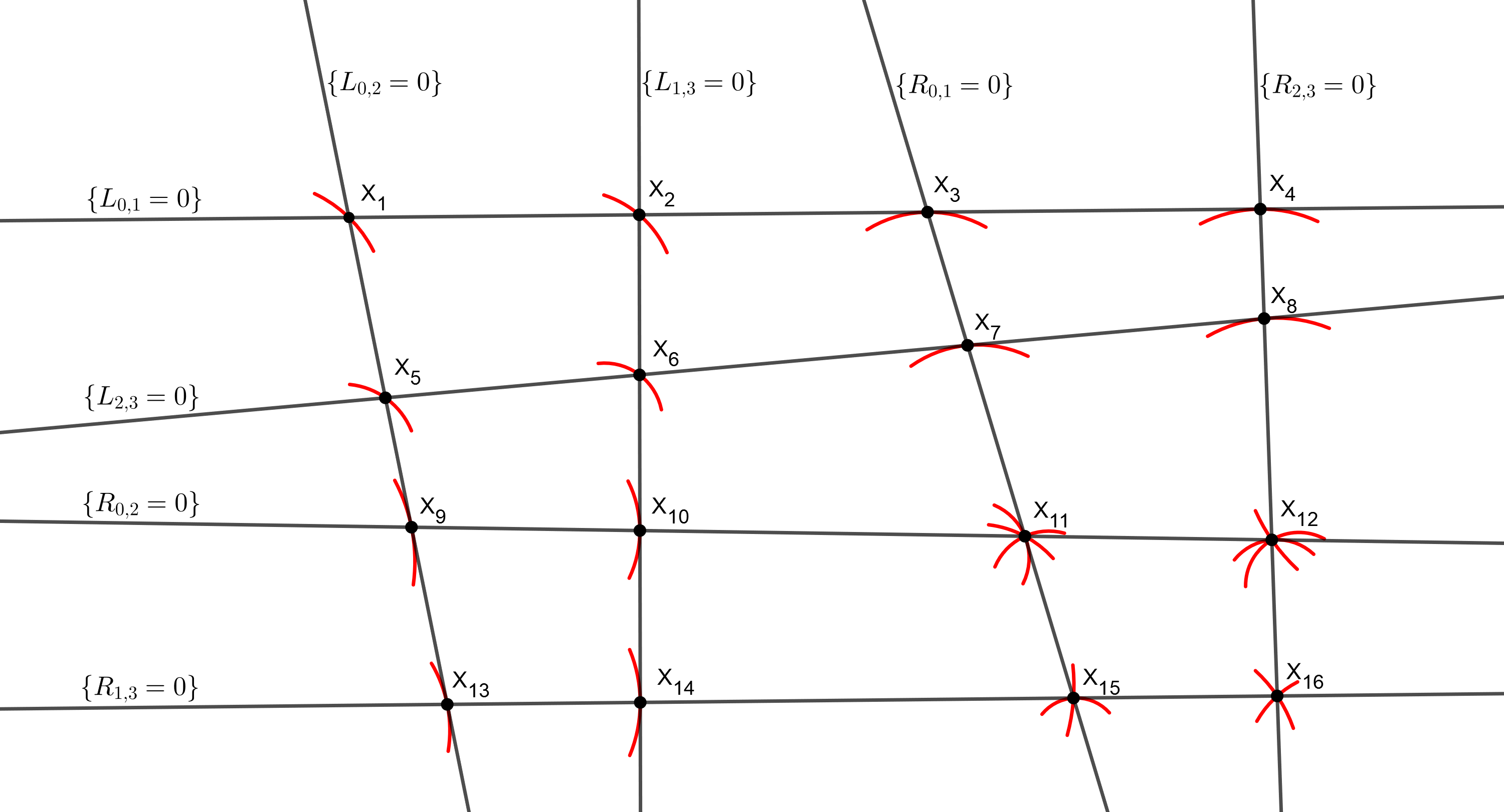
Figure 1: The intersections $X_{i}$ of the curve $\mathcal{B}_{P}$ with certain lines $L_{i,j},R_{i,j}$.

Claim 9.2.3

Consider the lines $\{L_{i,j}=0\}$ and $\{R_{i,j}=0\}$ and the points $X_{i}$ in Figure 1. For all but at most $450$ choices of $P\in E(k)$, those lines are distinct and the points $X_{i}$ are distinct.

Proof.

First we see that the points $\sigma^{0}Q,\sigma^{0}R,\ldots$, $\sigma^{3}Q,\sigma^{4}R$ are pairwise distinct: clearly $\sigma^{0}Q,\ldots$, $\sigma^{3}Q$ are distinct and $\sigma^{0}R,\ldots,\sigma^{3}R$ are distinct and if we had $\sigma^{i}Q=\sigma^{j}R$, then, for $l:=[k:\mathbb{F}_{q}]$ and $m:=i{-}j$, we would have

$$Q+P_{0}=\phi(R)= \phi(\sigma^{{i-j}}Q)=\phi(\phi^{l(i-j)}Q)=\phi^{lm+1}(Q)\implies\quad\phi^{4}(Q)=\phi^{4(lm+1)}(Q)=Q+4P_{0}\,,$$

which is absurd because $R$ is not a trap and consequently $\phi^{4}(Q)\neq Q+4P_{0}$.

If the lines $\{L_{0,2}=0\}$ and $\{L_{1,3}=0\}$ were equal, then the matrix of their coefficients

$$n(P)=\left(\begin{matrix}l_{2}{-}l_{0}&(f_{Q}{-}f_{\sigma^{2}Q})(P)&(l_{2}f_{Q}{-}l_{0}f_{\sigma^{2}Q})(P)\\ l_{3}{-}l_{1}&(f_{\sigma Q}{-}f_{\sigma^{3}Q})(P)&(l_{3}f_{\sigma Q}{-}l_{1}f_{\sigma^{3}Q})(P)\end{matrix}\right)$$

would have rank $1$, which, computing the deteminant of a submatrix of $n$, would imply $P$ to be a zero of the rational function $(l_{0}-l_{2})(f_{\sigma^{3}Q}{-}f_{\sigma Q})-(l_{1}{-}l_{3})(f_{\sigma^{2}Q}{-}f_{Q})$, that has five poles counted with multiplicity, since the points $Q,\ldots,\sigma^{3}Q$ are distinct and since $l_{i}\neq l_{j}$ by the choice of $\widetilde{P}$. Hence for all but at most five choices of $P\in E(k)$, the matrix $n(P)$ has rank $2$ and consequently the lines $\{L_{0,2}=0\}$ and $\{L_{1,3}=0\}$ are distinct.

Similar arguments prove that, for any other pair of lines $\Lambda,\Lambda^{\prime}$ in Figure 1, $\Lambda\neq\Lambda^{\prime}$ for all but at most five choices of $P$. We now prove that, for all $i\neq j$, we have $X_{i}\neq X_{j}$, for all but six choices of $P\in E(k)$. We treat only a couple of cases.

If $X_{9}=X_{12}$, then the lines $\{R_{0,2}=0\}$, $\{R_{2,3}=0\}$ and $\{L_{0,2}=0\}$ are concurrent, hence the following matrix, that contains their coefficients, is not invertible

$$M=M(P)=\left(\begin{matrix}r_{2}{-}r_{0}&(f_{R}{-}f_{\sigma^{2}R})(P)&(r_{2}f_{R}{-}r_{0}f_{\sigma^{2}R})(P)\\ r_{3}{-}r_{2}&(f_{\sigma^{2}R}{-}f_{\sigma^{3}R})(P)&(r_{3}f_{\sigma^{2}R}{-}r_{2}f_{\sigma^{3}R})(P)\\ l_{2}{-}l_{0}&(f_{Q}{-}f_{\sigma^{2}Q})(P)&(l_{2}f_{Q}{-}l_{0}f_{\sigma^{2}Q})(P)\\ \end{matrix}\right)\,,$$

implying that $P$ is a zero of the rational function $\det(M)$. Writing out $\det(M)$, and using that $\sigma^{0}Q,\sigma^{0}R,\ldots$, $\sigma^{3}Q,\sigma^{4}R$ are pairwise distinct, we see that there is a rational function $g$, regular in ${-}\sigma^{2}R$, such that

$$\det(M)=(l_{2}{-}l_{0})(r_{0}{-}r_{3})f_{\sigma^{2}R}^{2}+f_{\sigma^{2}R}\,g\,.$$

Since $l_{0}\neq l_{2}$ and $r_{0}\neq r_{3}$, the rational function $\det(M)$ has a pole of order $2$ in ${-}\sigma^{2}R$ and in particular $\det(M)$ is a non-zero rational function with at most $6$ poles counted with multiplicity. Hence $\det(M)$ has at most $6$ zeroes, implying that $X_{9}\neq X_{12}$, for all but $6$ choices of $P\in E(k)$.

If $X_{3}=X_{7}$, then the lines $\{L_{0,1}=0\}$, $\{L_{2,3}=0\}$ and $\{R_{0,1}=0\}$ are concurrent, hence the following matrix, that contains the coefficients of $L_{0,1}$, $L_{2,3}$ and $R_{0,1}$, is not invertible

$$N=N(P)=\left(\begin{matrix}l_{1}{-}l_{0}&(f_{Q}{-}f_{\sigma Q})(P)&(l_{1}f_{Q}{-}l_{0}f_{\sigma Q})(P)\\ l_{3}{-}l_{2}&(f_{\sigma^{2}Q}{-}f_{\sigma^{3}Q})(P)&(l_{3}f_{\sigma^{2}Q}{-}l_{2}f_{\sigma^{3}Q})(P)\\ r_{1}{-}r_{0}&(f_{R}{-}f_{\sigma R})(P)&(r_{1}f_{R}{-}r_{0}f_{\sigma R})(P)\\ \end{matrix}\right)\,.$$

As before, in order to prove that $X_{3}\neq X_{4}$ for all but at most $6$ choices of $P\in E(k)\setminus\{O_{E}\}$ it is enough proving that $\det(N(P))$, considered as a rational function of $P$, is not identically zero. We suppose by contradiction that $\det(N)$ is identically zero. Denoting $N_{i,j}$ the $(i,j)$-minor of $N(P)$, it easy to see the rational functions $N_{i,3}$ are not null. Consequently, the only way for $\det(N)$ to be zero is that the third column $N$ is linearly dependent from the first two. Hence, there are rational functions $A,B\in\overline{\mathbb{F}_{q}}(E)$ such that

$(\mathrm{9.2.4})$ $$\begin{cases}\big{(}l_{1}{-}l_{0}\big{)}\cdot A+\big{(}f_{Q}{-}f_{\sigma Q}\big{)}\cdot B=l_{1}f_{Q}{-}l_{0}f_{\sigma Q}\\ \big{(}l_{3}{-}l_{2}\big{)}\cdot A+\big{(}f_{\sigma^{2}Q}{-}f_{\sigma^{3}Q}\big{)}\cdot B=l_{3}f_{\sigma^{2}Q}{-}l_{2}f_{\sigma^{3}Q}\\ \big{(}r_{1}{-}r_{0}\big{)}\cdot A+\big{(}f_{R}{-}f_{\sigma R}\big{)}\cdot B=r_{1}f_{R}{-}r_{0}f_{\sigma R}\\ \end{cases}$$

and, using Cramer’s rule, we have

$$B=\frac{N_{1,2}}{N_{1,3}}=\frac{N_{2,2}}{N_{2,3}}=\frac{N_{3,2}}{N_{3,3}}\,.$$

We easily compute the poles of the rational functions $N_{i,j}$ and check that they all vanish in $\widetilde{P}$ and $O_{E}$, (for $O_{E}$ it is enough noticing that $(f_{P}{-}\tfrac{y}{x})(O_{E})=0$ for all $P\in E(\overline{\mathbb{F}_{q}})\setminus\{O_{E}\}$). These computations give

$$\mathrm{div}(N_{1,j}) =D_{1,j}+\widetilde{P}+O_{E}-({-}R)-({-}\sigma R)-({-}\sigma^{2}Q)-({-}\sigma^{3}Q)\,,$$

$$\mathrm{div}(N_{2,k}) =D_{2,j}+\widetilde{P}+O_{E}-({-}Q)-({-}\sigma Q)-({-}R)-({-}\sigma R)\,,$$

$$\mathrm{div}(N_{3,j}) =D_{3,j}+\widetilde{P}+O_{E}-({-}Q)-({-}\sigma Q)-({-}\sigma^{2}Q)-({-}\sigma^{3}Q)\,,$$

for certain positive divisors $D_{i,j}$ of degree $2$. Consequently

$$\mathrm{div}(B)=D_{1,2}-D_{1,3}=D_{2,2}-D_{2,3}=D_{3,2}-D_{3,3}\,.$$

Since the functions $f_{Q}$, $f_{\sigma Q}$, $f_{\sigma^{2}Q}$ and $f_{\sigma^{3}Q}$ are $\overline{\mathbb{F}_{q}}$-linearly independent, then $N_{1,2}$ and $N_{1,3}$ are not $\overline{\mathbb{F}_{q}}$-multiples and $B$ is not constant. Since every non-constant rational function on $E$ has at least two poles, we deduce that $D_{1,3}=D_{2,3}=D_{3,3}$ is the divisor of poles of $B$. In particular, in the group $E(\overline{\mathbb{F}_{q}})$, the sum of the poles of $N_{1,3}$ is equal to the sum of the poles of $N_{2,3}$ and to the sum of the poles of $N_{3,3}$. Writing it out, we get the following equalities in the group $E(\overline{\mathbb{F}_{q}})$

$$Q+\sigma Q=\sigma^{2}Q+\sigma^{3}Q=R+\sigma R\,.$$

Hence, using ($(\mathrm{8.2.1})$), ${-}Q{-}\sigma Q$ is a zero of $N_{3,3}$ and consequently the two poles of $B$ are ${-}Q{-}\sigma Q$ and ${-}Q{-}\sigma Q{-}\widetilde{P}$. By looking at ($(\mathrm{9.2.4})$), we deduce that $A$ has exactly one simple pole, namely ${-}Q{-}\sigma Q{-}\widetilde{P}$, which is absurd. Hence $\det(N(P))$ is not identically zero. ∎

We now study the geometrically irreducible components of $\mathcal{B}_{P}$ for the points $P$ such that the conclusions of Claim 9.2.3 hold (there are such $P$’s because $450$ is way smaller than $\#E(k)$). Equation ($(\mathrm{9.2.2})$), that defines $\mathcal{B}_{P}$, gives the following divisor-theoretic intersection

$(\mathrm{9.2.5})$ $$\mathcal{B}_{P}\cap\{L_{0,2}=0\}=X_{1}+X_{5}+qX_{9}+qX_{13}\,.$$

Since $X_{i}$’s are distinct, the point $X_{1}$ has multiplicity $1$ in the above intersection and consequently it is a smooth point of $\mathcal{B}_{P}$. With analogous arguments we see that all the points $X_{i}$, except the ones of shape $\{R_{i,j}=0\}\cap\{R_{l,m}=0\}$, are smooth. This is used in the following Claim.

Claim 9.2.6

Assuming the conclusions of Claim 9.2.3, the curve $\mathcal{B}_{P}$ does not contain any conic defined over $k$.

Proof.

Suppose there exists such a conic $\mathcal{Q}$. Since $X_{9}$ is a smooth point of $\mathcal{B}_{P}$, if $X_{9}\in\mathcal{Q}$, then $\mathcal{Q}$ is the only component of $\mathcal{B}_{P}$ passing through $X_{9}$, hence $X_{9}$ appears in $\mathcal{B}_{P}\cap\{L_{0,2}=0\}$ with multiplicity at most $2<q$, contradicting Equation ($(\mathrm{9.2.5})$). Hence $\mathcal{Q}$ does not contain $X_{9}$ nor, by a similar argument, $X_{13}$. This, together with Equation ($(\mathrm{9.2.5})$), implies that $X_{1}$ and $X_{5}$ belong to $\mathcal{Q}$. Analogously $X_{2}$ and $X_{6}$ belong to $\mathcal{Q}$.

We notice that $X_{1},X_{2},X_{5},X_{6}$ are in general position (by Claim 9.2.3) and that we know two conics passing through them, namely $\{L_{0,1}L_{2,3}=0\}$ and $\{L_{0,2}L_{1,3}=0\}$. Hence, if we choose a homogenous quadratic polynomial $F\in k[\alpha,\beta,\gamma]$ defining $\mathcal{Q}$, there are $\lambda_{0},\lambda_{1}\in\overline{\mathbb{F}_{q}}$ such that

$$F=\lambda_{0}L_{0,1}L_{2,3}+\lambda_{1}L_{0,2}L_{1,3}\,.$$

Our claim now follows by extending extend $\sigma$ to an element in $\mathrm{Gal}(\overline{\mathbb{F}_{q}}/k)$ and looking at its action on the above equation. For each $i,j\in\{0,1,2,3\}$ we have $\sigma L_{i,j}=L_{i+1,j+1}={-}L_{j+1,i+1}$, considering the indices modulo $4$, hence

$$\lambda_{0}L_{0,1}L_{2,3}+\lambda_{1}L_{0,2}L_{1,3}=F=\sigma F=\sigma(\lambda_{0})L_{2,3}L_{3,0}+\sigma(\lambda_{1})L_{0,2}L_{1,3}\,.$$

Some cumbersome computations imply that $\{L_{1,2}=0\}$ is the line through $X_{2},X_{5}$, while $\{L_{3,0}=0\}$ is the line through $X_{1},X_{6}$. In particular, the polynomials $L_{i,j}$ in the above equation are pairwise coprime, which implies $\lambda_{0}=\sigma(\lambda_{0})=0$. Hence, $\mathcal{Q}=\{F=0\}=\{L_{0,2}L_{1,3}=0\}$, which is absurd because $\{L_{0,2}L_{1,3}=0\}$ is not contained in $\mathcal{B}_{P}$. ∎

Claim 9.2.6 also implies that $\mathcal{B}_{P}$ does not contain a line of $\mathbb{P}^{2}$. Suppose that $\Lambda$ is a line contained in $\mathcal{B}_{P}$. Neither $X_{9}$ nor $X_{13}$ are contained in $\Lambda$ since they are smooth points of $\mathcal{B}_{P}$ and, by Equation ($(\mathrm{9.2.5})$, the unique components of $\mathcal{B}_{P}$ passing through them must have degree at least $q$ inside $\mathbb{P}^{2}$. Hence $\Lambda\cap\{L_{0,2}=0\}\in\{X_{1},X_{5}\}$ and consequently

$(\mathrm{9.2.7})$ $$(\Lambda\cup\sigma^{2}\Lambda)\cap\{L_{0,2}=0\}=X_{1}+X_{5}\,.$$

This implies that $\sigma^{2}\Lambda\neq\Lambda$ and that $\sigma^{2}\Lambda$ and $\Lambda$ are all the $\mathrm{Gal}(\overline{\mathbb{F}_{q}}/k)$-conjugates of $\Lambda$: if $\Lambda$ had another conjugate $\Lambda^{\prime}$, then, since $\mathcal{B}_{P}$ is defined over $k$, also $\Lambda^{\prime}$ would be a component of $\mathcal{B}_{P}$ and, by the same argument as before, $\Lambda^{\prime}\cap\{L_{0,2}=0\}=X^{\prime}\in\{X_{1},X_{5}\}$, which, together with Equation ($(\mathrm{9.2.7})$), implies that two or more components of $\mathcal{B}_{P}$ pass through $X^{\prime}$, contradicting the smoothness of $X_{1}$ and $X_{5}$. We deduce that $\Lambda{\cup}\sigma^{2}\Lambda$ is a conic defined over $k$ and contained in $\mathcal{B}_{P}$, contradicting Claim 9.2.6.

By a similar argument, no conic $\mathcal{Q}$ is a component of $\mathcal{B}_{P}$: if this happens, since conics have degree $2<q$ in $\mathbb{P}^{2}$, then $X_{9},X_{13}$ do not belong to any of the $\mathrm{Gal}(\overline{\mathbb{F}_{q}}/k)$-conjugates of $\mathcal{Q}$, thus, by Equation ($(\mathrm{9.2.5})$), for all $\tau\in\mathrm{Gal}(\overline{\mathbb{F}_{q}}/k)$ we have

$$\tau(\mathcal{Q})\cap\{L_{0,2}=0\}=X_{1}+X_{5}=\mathcal{Q}\cap\{L_{0,2}=0\}$$

hence, by the smoothness of $X_{1}$ and $X_{5}$, $\mathcal{Q}$ is defined over $k$, contradicting Claim 9.2.6.

We now suppose that $\mathcal{B}_{P}$ is not geometrically irreducible. Let $\mathcal{B}_{1},\ldots,\mathcal{B}_{r}$ be the geometrically irreducible components of $\mathcal{B}_{P}$. As we already proved, each $\mathcal{B}_{i}$ has degree at least $3$, hence the intersection $\mathcal{B}_{i}\cap\{L_{0,2}=0\}$ is a sum of at least $3$ points counted with multiplicity. By Equation ($(\mathrm{9.2.5})$), this implies that $\mathcal{B}_{i}$ is passing through $X_{9}$ or $X_{13}$ hence each $\mathcal{B}_{i}$ has degree at least $q$. Since the sum of the degrees of the $\mathcal{B}_{i}$’s is equal to $2q{+}2<3q$, we deduce that $r=2$ and that either $\deg(\mathcal{B}_{1})=\deg(\mathcal{B}_{2})=q+1$ or, up to reordering, $\deg(\mathcal{B}_{1})=q$ and $\deg(\mathcal{B}_{2})=q+2$.

If $\deg(\mathcal{B}_{1})=\deg(\mathcal{B}_{2})=q+1$, Equation ($(\mathrm{9.2.5})$) implies that, up to reordering, $X_{1}\in\mathcal{B}_{1}(\overline{\mathbb{F}_{q}})$ and $X_{5}\in\mathcal{B}_{2}(\overline{\mathbb{F}_{q}})$. Since $\mathcal{B}_{P}$ is defined over $k$, then $\mathrm{Gal}(\overline{\mathbb{F}_{q}}/k)$ acts on $\{\mathcal{B}_{1},\mathcal{B}_{2}\}$ and because of the cardinality of such a set, then $\sigma^{2}$ acts trivially. In particular $X_{5}=\sigma^{2}X_{1}$ belongs to $\sigma^{2}\mathcal{B}_{1}(\overline{\mathbb{F}_{q}})=\mathcal{B}_{1}(\overline{\mathbb{F}_{q}})$, hence $X_{5}\in\mathcal{B}_{1}(\overline{\mathbb{F}_{q}})\cap\mathcal{B}_{2}(\overline{\mathbb{F}_{q}})$, contradicting the smoothness of $X_{5}$. This contradiction implies that

$$\deg(\mathcal{B}_{1})=q,\quad\deg(\mathcal{B}_{2})=q+2\,.$$

For each $i\in\{1,2\}$ let $M_{i}\in\overline{\mathbb{F}_{q}}[\alpha,\beta,\gamma]$ be a homogeneous polynomial defining $\mathcal{B}_{i}$.

Claim 9.2.8

There exists homogenous polynomials $F_{1},F_{2},G_{2},N_{1},N_{2}\in\overline{\mathbb{F}_{q}}[\alpha,\beta,\gamma]$ of respective degree $1,1,1,q-4,q-2$ such that

(9.2.9) $$M_{1} =F_{1}^{q}+L_{0,1}L_{2,3}L_{0,2}L_{1,3}N_{1},$$

(9.2.10) $$M_{2} =F_{2}^{q}L_{0,1}L_{2,3}+G_{2}^{q}L_{0,2}L_{1,3}+L_{0,1}L_{2,3}L_{0,2}L_{1,3}N_{2}$$

Proof.

We start from the first part. Since $\deg\mathcal{B}_{1}=q$ and since $X_{1},X_{5},X_{9}$ and $X_{13}$ are smooth, Equation ($(\mathrm{9.2.5})$) implies that $\mathcal{B}_{1}\cap\{L_{0,2}=0\}$ is either $qX_{13}$ or $qX_{9}$. Hence $M_{1}\bmod{L_{0,2}}$ is a $q$-th power, i.e. there are homogeneous polynomials $A_{1},B_{1}$, with $A_{1}$ linear, such that

$$M_{1}=A_{1}^{q}+B_{1}L_{0,2}\,.$$

Similarly to $\mathcal{B}_{1}\cap\{L_{0,2}=0\}$, we have that $\mathcal{B}_{1}\cap\{L_{1,3}=0\}$ is either $qX_{14}$ or $qX_{10}$, hence there exists a linear polynomial $A_{2}$ such that

(9.2.11) $$A_{2}^{q}\equiv M_{1}\equiv A_{1}^{q}+B_{1}L_{0,2}\pmod{L_{1,3}}\quad\implies\quad B_{1}L_{0,2}\equiv(A_{2}-A_{1})^{q}\pmod{L_{1,3}}$$

We notice, that, since $L_{1,3}=l_{\alpha}\alpha+l_{\beta}\beta+l_{\gamma}\gamma$ is linear, with $l_{\alpha}=l_{3}-l_{1}\neq 0$, the map $F\mapsto F\left(-\frac{l_{\beta}\beta+l_{\gamma}\gamma}{l_{\alpha}},\beta,\gamma\right)$ gives an isomorphism of $\overline{\mathbb{F}_{q}}[\alpha,\beta,\gamma]/L_{1,3}$ with $\overline{\mathbb{F}_{q}}[\beta,\gamma]$, which is a UFD. Moreover this isomorphism sends $(A_{2}{-}A_{1})\bmod{L_{1,3}}$ to a homogeneous polynomial of degree at most $1$, which means that $(A_{2}{-}A_{1})\bmod{L_{1,3}}$ is either null or irreducible. We deduce that, in the last congruence of (9.2.11), either both sides are zero or the right hand side gives the prime factorization of the left hand side. In both cases we have $B_{1}\equiv\lambda_{1}L_{0,2}^{q-1}$ for some $\lambda_{1}\in\overline{\mathbb{F}_{q}}$, hence

$$B_{1}=\lambda_{1}L_{0,2}^{q-1}+B_{2}L_{1,3}\quad\implies M_{1}=(A_{1}+\lambda_{1}L_{0,2})^{q}+B_{2}L_{0,2}L_{0,3}=A_{3}^{q}+B_{2}L_{0,2}L_{0,3}$$

for certain homogeneous polynomials $A_{3},B_{2}$, with $A_{3}$ linear. Again, $\mathcal{B}_{1}\cap\{L_{0,1}=0\}$ is either $qX_{3}$ or $qX_{4}$, hence, for a some linear homogenous polynomial $A_{4}$, we have

$$A_{4}^{q}\equiv M_{1}\equiv A_{3}^{q}+B_{2}L_{0,2}L_{1,3}\pmod{L_{0,1}}\quad\implies\quad B_{2}\,L_{0,2}\,L_{1,3}\equiv(A_{4}-A_{3})^{q}\pmod{L_{0,1}}\,.$$

As before, the last congruence can be interpreted as an equation in the UFD $\overline{\mathbb{F}_{q}}[\alpha,\beta,\gamma]/L_{1,3}$ and, since $(A_{4}{-}A_{3})\bmod{L_{0,1}}$ is either irreducible or null, then either both sides are zero or the right hand side gives the prime factorization of the left hand side. The latter is not possible, since the points $X_{1}=\{L_{0,1}=0\}\cap\{L_{0,2}=0\}$ and $X_{2}=\{L_{0,1}=0\}\cap\{L_{1,3}=0\}$ are distinct and consequently $L_{0,2}\bmod{L_{0,1}}$ and $L_{1,3}\bmod{L_{0,1}}$ are relatively prime. We deduce that $B_{2}$ is divisible by $L_{0,1}$. By a similar argument $B_{2}$ is also divisible by $L_{2,3}$, hence Equation (9.2.9).

We now turn to (9.2.10). Since $\deg\mathcal{B}_{2}=q+2$ and since $X_{1},X_{5},X_{9}$ and $X_{13}$ are smooth, Equation ($(\mathrm{9.2.5})$) implies that $\mathcal{B}_{2}\cap\{L_{0,2}\}$ is either $X_{1}{+}X_{5}{+}qX_{13}$ or $X_{1}{+}X_{5}{+}qX_{9}$, hence we can write $M_{2}=A_{5}^{q}L_{0,1}L_{2,3}+B_{3}L_{0,2}$ for some homogeneous polynomials $A_{5},B_{3}$, with $A_{5}$ linear. In a similar fashion, $\mathcal{B}_{2}\cap\{L_{1,3}\}$ is either $X_{2}{+}X_{6}{+}qX_{14}$ or $X_{2}{+}X_{6}{+}qX_{10}$, hence,

$$L_{0,1}L_{2,3}A_{6}^{q}\equiv M_{1}\equiv L_{0,1}L_{2,3}A_{5}^{q}+B_{3}L_{0,2}\,(\bmod{L_{1,3}})\,\implies\,B_{3}L_{0,2}\equiv L_{0,1}L_{2,3}(A_{6}-A_{5})^{q}\,(\bmod{L_{1,3}})$$

As before, in the last equation either both sides are zero or the right hand side gives the prime factorization of the left hand side. In both cases $B_{3}$ is congruent to a scalar multiple of $L_{0,1}L_{2,3}L_{0,2}^{q-1}$: if $B_{3}\equiv 0$ this is obvious, otherwise we need to use that the polynomials $L_{0,1}$, $L_{2,3}$ and $L_{0,2}$ are relatively prime modulo $L_{1,3}$ because the lines $\{L_{0,1}=0\}$, $\{L_{2,3}=0\}$ and $\{L_{0,2}=0\}$ all have different intersection with $\{L_{1,3}=0\}$. Hence

$$M_{2}=A_{7}^{q}L_{0,2}L_{1,3}+B_{4}L_{0,1}L_{2,3}.$$

for certain $A_{7},B_{4}\in\overline{\mathbb{F}_{q}}[\alpha,\beta,\gamma]$. Iterating similar arguments we prove Equation 9.2.10. ∎

Let $F_{1},F_{2},G_{1},N_{1}$ and $N_{2}$ as in Claim 9.2.8. Up to multiplying $M_{1}$ with an element of $\overline{\mathbb{F}_{q}}^{\times}$, we can suppose that $M=M_{1}M_{2}$. Reducing this equality modulo $L_{0,2}L_{1,3}$ we see that

$$L_{0,2}L_{1,3}\text{ divides }L_{0,1}L_{2,3}(F_{1}F_{2}+R_{0,2}R_{1,3})^{q}.$$

Since the $L_{i,j}$’s in the above equation are coprime, $L_{0,2}L_{1,3}$ divides $F_{1}F_{2}{+}R_{0,2}R_{1,3}$. Since $F_{1}F_{2}{+}R_{0,2}R_{1,3}$ is homogenous of degree at most $2$, then it is a scalar multiple of $L_{0,2}L_{1,3}$. Using a similar argument with $L_{0,1}L_{2,3}$ we prove that there exist $\lambda,\mu\in\overline{\mathbb{F}_{q}}$ such that

(9.2.12) $$F_{1}F_{2}+R_{0,2}R_{1,3}=\lambda L_{0,2}L_{1,3},\quad F_{1}G_{2}-R_{0,1}R_{2,3}=\mu L_{0,1}L_{2,3}\,.$$

We have $\lambda\neq 0$, otherwise $F_{1}$ would be a scalar multiple of either $R_{0,2}$ or $R_{1,3}$: in the first case Equation 9.2.9 would imply that $\mathcal{B}_{1}$ contains $X_{9}$ but not $X_{14}=\tau(X_{9})$, implying that $\tau(\mathcal{B}_{1})$ is a component of $\mathcal{B}$ different from $\mathcal{B}_{1}$, that is $\tau(\mathcal{B}_{1})=\mathcal{B}_{2}$ which contradicts the inequality $\deg(\mathcal{B}_{2})>\deg(\mathcal{B}_{1})$; in the second case Equation 9.2.9 would imply that $\mathcal{B}_{1}$ contains $X_{13}$ but not $X_{10}=\tau(X_{13})$, leading to the same contradiction.

Using Equations (9.2.9), (9.2.10) and (9.2.12) and the equality $M_{1}M_{2}{=}M$, we see that

(9.2.13) $$0 =\frac{M_{1}M_{2}-M}{L_{0,1}L_{2,3}L_{0,2}L_{1,3}}=$$

$$=\mu^{q}\!L_{0,1}^{q-1}\!L_{2,3}^{q-1}{+}\lambda^{q}\!L_{0,2}^{q-1}\!L_{1,3}^{q-1}{+}F_{1}^{q}\!N_{2}{+}F_{2}^{q}\!N_{1}\!L_{0,1}\!L_{2,3}{+}G_{2}^{q}\!N_{1}\!L_{0,2}\!L_{1,3}{+}N_{1}\!N_{2}\!L_{0,1}\!L_{2,3}\!L_{0,2}\!L_{1,3}$$

$$\equiv\lambda^{q}(L_{0,2}L_{1,3})^{q-1}+F_{1}^{q}N_{2}+G_{2}^{q}N_{1}L_{0,2}L_{1,3}\pmod{L_{0,1}}.$$

As already observed in the proof of Claim 9.2.8, $\overline{\mathbb{F}_{q}}[\alpha,\beta,\gamma]/L_{0,1}$ is isomorphic to $\overline{\mathbb{F}_{q}}[\beta,\gamma]$ through the map $F\mapsto F\left(-\frac{l_{\beta}\beta+l_{\gamma}\gamma}{l_{\alpha}},\beta,\gamma\right)$, where $l_{\alpha},l_{\beta}$ and $l_{\gamma}$ are the coefficients of $L_{0,1}$. In particular, $\overline{\mathbb{F}_{q}}[\alpha,\beta,\gamma]/L_{0,1}$ is a UFD and for any $F\in\overline{\mathbb{F}_{q}}[\alpha,\beta,\gamma]/L_{0,1}$ we denote $\tilde{F}$ its image in $\overline{\mathbb{F}_{q}}[\beta,\gamma]$ through the above map. With this notation (9.2.13) implies that both $\tilde{L}_{0,2}$ and $\tilde{L}_{1,3}$ divide $\tilde{N}_{2}\tilde{F_{1}^{q}}$. More precisely $\tilde{L}_{0,2}$ and $\tilde{L}_{1,3}$ divide $\tilde{N}_{2}$, because $\tilde{F}_{1}$ is relatively prime with both $\tilde{L}_{0,2}$ and $\tilde{L}_{1,3}$, since $\mathcal{B}_{1}\cap L_{0,1}$ does not contain $X_{1}=\{L_{0,2}{=}0\}\cap\{L_{0,1}{=}0\}$ nor $X_{3}=\{L_{1,3}{=}0\}\cap\{L_{0,1}{=}0\}$. Moreover, since $X_{1}=\{L_{0,2}{=}0\}\cap\{L_{0,1}{=}0\}$ and $X_{3}=\{L_{1,3}{=}0\}\cap\{L_{0,1}{=}0\}$ are distinct, $\tilde{L}_{0,2}$ is relatively prime with $\tilde{L}_{1,2}$ and we can write $\tilde{N}_{2}=\tilde{L}_{0,2}\tilde{L}_{1,3}N_{3}$ for some $N_{3}\in\overline{\mathbb{F}_{q}}[\beta,\gamma]$. Substituting in (9.2.13) we get

$$\lambda^{q}\tilde{L}_{0,2}^{q-2}\tilde{L}_{1,3}^{q-2}+\tilde{F}_{1}^{q}N_{3}+\tilde{G}_{2}^{q}\tilde{N}_{1}=0.$$

Since $\tilde{L}_{0,2}$ and $\tilde{L}_{1,2}$ are coprime and since $\lambda\neq 0$, this contradicts Lemma 9.2.14 below.

In particular the assumption of the reducibility of $\mathcal{B}$, together with the conclusions of Claim 9.2.3, led to contradiction. We deduce that for all but at most $450$ choices of $P\in E(k)$ the curve $\mathcal{B}_{P}$ is geometrically irreducible. Since $\#E(k)>450$ and since all the components of $\mathcal{B}$ project surjectively to $E$, we deduce that $\mathcal{B}$ is reduced and geometrically irreducible.

Lemma 9.2.14

Let $L_{1},L_{2}\in\overline{\mathbb{F}_{q}}[\beta,\gamma]$ be relatively prime homogenous linear polynomials. Then, there exist no homogenous polynomial $A,B,C,D\in\overline{\mathbb{F}_{q}}[\beta,\gamma]$ such that

$$L_{1}^{q-2}L_{2}^{q-2}=A^{q}B+C^{q}D.$$

Proof.

The zeroes of $L_{1}$ and $L_{2}$ in $\mathbb{P}^{1}$ are distinct, hence, up to a linear transformation we can suppose that their zeroes are $0$ and $\infty$. In particular, up to scalar multiples we can suppose $L_{1}=\beta$ and $L_{2}=\gamma$, implying that $A^{q}B+C^{q}D=\beta^{q-2}\gamma^{q-2}$. This is absurd because any monomial appearing in $A^{q}$ or in $B^{q}$ is either a multiple of $\beta^{q}$ of a multiple of $\gamma^{q}$, hence the same is true for all the monomials appearing in $A^{q}B+C^{q}D$. ∎

9.3 The irreducible components of $\mathcal{C}$

In this subsection we prove that all the geometrically irreducible components of $\mathcal{C}$ are defined over $k$. To do so, we can ignore ($(\mathrm{9.1.6})$) in the definition of $\mathcal{C}$. The strategy is applying Lemma 7.6 to the variety $\mathcal{B}$, using the rational functions

$$u_{1},u_{2},u_{3}\colon\mathcal{B}\dashrightarrow\mathbb{P}^{1}\,,\qquad u_{i}(\alpha,\beta,1,P)=f_{\alpha,\beta,P}(\sigma^{i-1}Q)\,,$$

$$w_{1},w_{2},w_{3}\colon\mathcal{B}\dashrightarrow\mathbb{P}^{1}\,,\qquad w_{i}(\alpha,\beta,1,P)=-f_{\alpha,\beta,P}(\sigma^{i-1}R)\,,$$

and the irreducible divisor $Z\subset\mathcal{B}$ being the Zariski closure of

$(\mathrm{9.3.1})$ $$\left\{(\alpha,\beta,P)\in(\mathbb{A}^{2}{\times}E^{\prime})(\overline{\mathbb{F}_{q}}):\begin{matrix}P=-Q-\sigma Q-\sigma^{3}Q-\widetilde{P}\,,\\ \alpha=\big{(}(f_{Q}(P){-}f_{\sigma Q}(P))\beta+l_{1}f_{Q}(P){-}l_{0}f_{\sigma Q}(P)\big{)}/(l_{0}{-}l_{1})\end{matrix}\right\}.$$

Claim 9.3.2

The variety $Z$ is generically contained in the smooth locus of $\mathcal{B}$ and the rational function $u_{1}{-}u_{2}$ vanishes on $Z$ with multiplicity $1$.

Proof.

We restrict to an open subset $U\subset\mathbb{P}^{2}\times E$ containing the generic point of $Z$. Up to shrinking $U$, the rational functions $u_{i},w_{i}$ can be extended to regular functions on $U$ using the definition ($(\mathrm{9.1.1})$) of $f_{\alpha,\beta,P}$, and we have

$$u_{1}-u_{2} =\frac{L_{0,1}(\alpha,\beta,1,P)}{\big{(}l_{0}+\beta\big{)}\big{(}l_{1}+\beta\big{)}}\,,$$

where $L_{i,j}(\alpha,\beta,\gamma,P)\in\overline{\mathbb{F}_{q}}[U]$ is defined as in ($(\mathrm{9.2.1})$), as well as $R_{i,j}(\alpha,\beta,\gamma,P)$. Since we can assume that $l_{0}{+}\beta,l_{1}{+}\beta$ are invertible on $U$ and since $Z$ is generically smooth, it is enough showing that $Z\cap U$ is a component of $(\mathcal{B}\cap U)\cap{\{L_{0,1}=0\}}$ having multiplicity one. Up to shrinking $U$, the $\mathcal{B}\cap U$ is the vanishing locus, inside $U$, of

$$M(\alpha,\beta,P):=(L_{0,2}L_{1,3}R_{0,1}^{q}R_{2,3}^{q}-L_{0,1}L_{2,3}R_{0,2}^{q}R_{1,3}^{q})(\alpha,\beta,1,P)\quad\in\overline{\mathbb{F}_{q}}[U]\,.$$

Since the restriction of $M$ to $\{L_{0,1}=0\}$ is equal to the restriction of $L_{0,2}L_{1,3}R_{0,1}^{q}R_{2,3}^{q}$, it is enough showing that $L_{0,2}$, $R_{0,1}$, $R_{2,3}$ do not vanish on $Z$ and that $\{L_{1,3}=0\}\cap\{L_{0,1}=0\}$ contains $Z\cap U$ with multiplicity $1$. We start from the latter. Eliminating the variable $\alpha$ we see that, up to shrinking $U$, $\{L_{1,3}=0\}\cap\{L_{0,1}=0\}$ is defined by the equations

$(\mathrm{9.3.3})$ $$\lambda(P)=0\quad\text{and}\quad(l_{1}-l_{0})\alpha+(f_{Q}(P)-f_{\sigma Q}(P))\beta+l_{1}f_{Q}(P)-l_{0}f_{\sigma Q}(P)=0\,,$$

where

$$\lambda(P):=(l_{1}{-}l_{0})f_{\sigma^{3}Q}(P)+(l_{3}{-}l_{1})f_{Q}(P)+(l_{0}{-}l_{3})f_{\sigma Q}(P)\quad\in\overline{\mathbb{F}_{q}}(E)\,.$$

The function $\lambda$ has three simple poles, namely ${-}Q,{-}\sigma Q,{-}\sigma^{3}Q$, and we easily verify that $\lambda(\widetilde{P})=\lambda(O_{E})=0$. We deduce that $P={-}Q{-}\sigma Q{-}\sigma^{3}Q{-}P_{0}$ is a simple zero of $\lambda$. This, together with the fact that the second equation in ($(\mathrm{9.3.3})$) is equal to the second equation in the definition ($(\mathrm{9.3.1})$) of $Z$, implies that $\{L_{1,3}=0\}\cap\{L_{0,1}=0\}$ contains $Z\cap U$ with multiplicity $1$.

We now suppose by contradiction that $R_{0,1}$ vanishes on $Z\cap U$. Substituting $\alpha$ and $P$ in $R_{0,1}$ as in the definition ($(\mathrm{9.3.1})$) of $Z$, we see that

$$R_{0,1}(\alpha,\beta,1,P)|_{Z\cap U}=\frac{\lambda_{0}({-}Q{-}\sigma Q{-}\sigma^{3}Q{-}\widetilde{P})}{l_{0}-l_{1}}\beta+\frac{\lambda_{1}({-}Q{-}\sigma Q{-}\sigma^{3}Q{-}\widetilde{P})}{l_{0}-l_{1}}\,,$$

where

$$\lambda_{0}(P):= (r_{1}-r_{0})(f_{Q}-f_{\sigma Q})(P)-(l_{1}-l_{0})(f_{R}-f_{\sigma R})(P)\,,$$

$$\lambda_{1}(P):= (r_{1}-r_{0})(l_{1}f_{Q}(P)-l_{0}f_{\sigma Q}(P))-(l_{1}-l_{0})(r_{1}f_{R}(P)-r_{0}f_{\sigma R}(P))\,,$$

and we deduce that both $\lambda_{0}$ and $\lambda_{1}$ vanish on $P={-}Q{-}\sigma Q{-}\sigma^{3}Q{-}\widetilde{P}$. Both $\lambda_{0}$ and $\lambda_{1}$ have $4$ poles and $4$ zeroes counted with multiplicity: they have the same poles they share three zeroes, namely $O_{E},\widetilde{P}$ and ${-}Q{-}\sigma Q{-}\sigma^{3}Q{-}\widetilde{P}$. Since, in the group on $E(\overline{\mathbb{F}_{q}})$, the sum of the zeroes of an element of $\overline{\mathbb{F}_{q}}(E)^{\times}$ is equal to the sum of the poles, then $\lambda_{0}$ and $\lambda_{1}$ also share the fourth zero, hence $\lambda_{0}$ and $\lambda_{1}$ differ by a multiplicative constant in $\overline{\mathbb{F}_{q}}$. This is absurd because $l_{0}\neq l_{1}$ and because the functions $f_{Q}$, $f_{\sigma Q}$, $f_{R}$, $f_{\sigma R}$ are $\overline{\mathbb{F}_{q}}$-independent.

A similar argument implies that $R_{2,3}$ does not vanish on $Z\cap U$, while the case of $L_{0,2}$ is easier. Substituting $\alpha$ and $P$ in $L_{0,2}(\alpha,\beta,1,P)$ as in the definition ($(\mathrm{9.3.1})$) of $Z$ we get

$$L_{0,2}(\alpha,\beta,1,P)|_{Z\cap U}=\frac{(\beta+l_{0})\lambda_{2}({-}Q{-}\sigma Q{-}\sigma^{3}Q{-}\widetilde{P})}{l_{0}-l_{1}}\,,$$

where

$$\lambda_{2}(P):=(l_{2}{-}l_{1})f_{Q}(P)+(l_{0}{-}l_{2})f_{\sigma Q}(P)+(l_{1}{-}l_{0})f_{\sigma^{2}Q}(P)\quad\in\overline{\mathbb{F}_{q}}(E)\,.$$

Analogously to $\lambda$, we see that the zeroes of $\lambda_{2}$ are $\widetilde{P},O_{E}$ and ${-}Q{-}\sigma Q{-}\sigma^{2}Q{-}P_{0}$, hence $\lambda_{2}$ does not vanish on ${-}Q{-}\sigma Q{-}\sigma^{3}Q{-}P_{0}$, implying that $L_{0,2}$ does not vanish on $Z\cap U$. ∎

We can show that $u_{2}{-}u_{3}$, $w_{3}{+}u_{3}$, $w_{3}{+}u_{1}$ and $w_{i}{-}w_{j}$ do not vanish on $Z$ using similar arguments to the ones used in the last part of the above proof. Hence, by Lemma 7.6, all the components of $\mathcal{C}$ are defined over $k$ and distinct.

9.4 $k$-rational points on $\mathcal{C}$

Finally we prove that $\#\mathcal{C}(k)$ is larger than $\tfrac{1}{2}(\#k)^{2}$. The surface $\mathcal{C}$ is contained in the open subset of $\mathbb{A}^{2}\times(E{\setminus}\{O_{E}\})\times\mathrm{PGL}_{2}\times\mathbb{A}^{1}$ made of points $(\alpha,\beta,(x,y),\left(\begin{smallmatrix}a&b\\ c&d\\ \end{smallmatrix}\right),z)$ such that $c\neq 0$. Hence $\mathcal{C}$ is contained in $\mathbb{A}^{8}$, with variables $\alpha,\beta$, $x,y$, $a,b,d$, $z$ and it is defined by the following equations:.

• $0=p_{1}:=W(x,y)$, the Weierstrass equation defining $E$;

• $0=p_{2}:=(d^{q}{-}a)^{q+1}(z^{q}{-}z)^{q^{2}{-}q}-(ad{-}b)^{q}(\tfrac{z^{q^{2}}{-}z}{z^{q}{-}z})^{q+1}$, the dehomogenization of ($(\mathrm{9.1.2})$) in $c$;

• $0=p_{i}(\alpha,\beta,x,y,a,b,d)$ for $i=3,4,5,6$, obtained by ($(\mathrm{9.1.3})$) after dehomogenizing in $c$, substituting $f_{\sigma^{i}Q},f_{\sigma^{i}R}$ by their expressions in $\alpha,\beta,x,y$ and clearing denominators;

• a number of conditions $0\neq q_{j}$ ensuring that $P\neq-\sigma^{i}Q,P\neq-\sigma^{i}R$, $\beta+f_{\widetilde{P}}(\sigma^{i}Q)\neq 0$, $\beta+f_{\widetilde{P}}(\sigma^{i}R)\neq 0$, $d^{q}-a\neq 0$, $ad-b\neq 0$, that ($(\mathrm{9.1.6})$) is satisfied, that $f_{\alpha,\beta,P}(\sigma^{i}Q)$ are distinct and that $f_{\alpha,\beta,P}(\sigma^{i}R)$ are distinct.

In particular, $\mathcal{C}$ can be seen as a closed subvariety of $\mathbb{A}^{9}$, with variables $\alpha,\beta$, $x,y$, $b,c,d,z$ and $t$ defined by the seven equations $p_{1}=0,\ldots,p_{6}=0$ and $0=p_{7}:=tq_{1}\cdots q_{r}-1$. Let $\mathcal{C}_{1},\ldots,\mathcal{C}_{s}$ be the geometrically irreducible components of $\mathcal{C}$. By [7, Remark $11.3$], we have

$(\mathrm{9.4.1})$ $$\#\mathcal{C}(k)\geq\#\mathcal{C}_{1}(k)\geq(\#k)^{2}-(\delta-1)(\delta-2)(\#k)^{\frac{3}{2}}-K(\mathcal{C}_{1})(\#k)\,,$$

where $\delta$ is the degree of $\mathcal{C}_{1}$ and $K(\mathcal{C}_{1})$ is the sum of the Betti numbers of $\mathcal{C}$ relative to the compact $\ell$-adic cohomology. Since $\mathcal{C}_{1}$ is a component of $\mathcal{C}$ then

$(\mathrm{9.4.2})$ $$\delta\leq\deg(p_{1})\cdots\deg(p_{7})\,.$$

Since $\mathcal{C}$ is the disjoint union of the $\mathcal{C}_{i}$, the Betti numbers of $\mathcal{C}$ are the sums of the Betti numbers of the $\mathcal{C}_{i}$. Hence, using [12, Corollary of Theorem 1]

$(\mathrm{9.4.3})$ $$K(\mathcal{C}_{1})\leq K(\mathcal{C})\leq 6\cdot 2^{7}\cdot\left(3+7\max_{i=1,\dots,7}\{\deg(p_{i})\}\right)^{10}\,.$$

Combining Equations ($(\mathrm{9.4.1})$), ($(\mathrm{9.4.2})$) and ($(\mathrm{9.4.3})$) and the inequalities $\deg p_{1}\leq 3$, $\deg p_{2}\leq q^{3}{+}q$, $\deg p_{3},\ldots,\deg p_{6}\leq 2q{+}3$, $\deg p_{7}\leq 16q^{2}{+}37q{+}75$, we deduce that $\#\mathcal{C}(k)>\tfrac{1}{2}(\#k)^{2}$ when $\#k\geq q^{80}$ and $q\geq 3$.

References

- [1] E. Berlekamp, Factoring polynomials over large finite fields. Math. Comp. 24 (1970), 713- 735.
- [2] R. Barbulescu , P. Gaudry, A. Joux, E. Thomé, A quasi-polynomial algorithm for discrete logarithm in finite fields of small characteristic. Annual International Conference on the Theory and Applications of Cryptographic Techniques (2014), 1-16.
- [3] A. W. Bluher, On . Finite Fields and Their Applications 10 (2004) No. 3, 285–305.
- [4] Q. Cheng, D. Wan, J. Zhuang, Traps to the BGJT-algorithm for discrete logarithms. LMS Journal of Computation and Mathematics 17 (2014), 218-229.
- [5] J. M. Couveignes, R. Lercier, Elliptic periods for finite fields. Finite Fields and Their Applications, 15 (2009) No. 1, 1–22.
- [6] W. Diffie, M. Hellman, New directions in cryptography. IEEE Trans. Inform. Theory 22 (1976).
- [7] S.R. Ghorpade, G. Lachaud, Étale cohomology, Lefschetz theorems and number of points of singular varieties over finite fields. Moscow Mathematical Journal 2 (2002) No. 3, 589-631.
- [8] R. Granger, T. Kleinjung, J. Zumbrägel, On the discrete logarithm problem in finite fields of fixed characteristic. Transactions of the American Mathematical Society 370 (2018) No. 5, 3129-3145.
- [9] A. Joux, A new index calculus algorithm with complexity L(1/4+o(1)) in small characteristic. Conference on Selected Areas in Cryptography (2013), 355-379.
- [10] A. Joux, C. Pierrot, Algorithmic aspects of elliptic bases in finite field discrete logarithm algorithms. arXiv preprint 1907.02689 (2019).
- [11] A. Joux, C. Pierrot, Improving the polynomial time precomputation of frobenius representation discrete logarithm algorithms - simplified setting for small characteristic finite fields. Advances in Cryptology - ASIACRYPT 2014 - 20th International Conference on the Theory and Application of Cryptology and Information Security, Kaoshiung, Taiwan, R.O.C., December 7-11, 2014. Proceedings, Part I, pages 378–397, 2014.
- [12] N. M. Katz, Sums of Betti numbers in arbitrary characteristic. Finite Fields and their Applications 7 (2001) No. 1, 29-44.
- [13] T. Kleinjung, B. Wesolowski, A new perspective on the powers of two descent for discrete logarithms in finite fields. The Open Book Series 2 (2019) No. 1, 343-352.
- [14] T. Kleinjung, B. Wesolowski, Discrete logarithms in quasi-polynomial time in finite fields of fixed characteristic. Journal of the American Mathematical Society 35.2 (2022): 581-624.
- [15] H.W. Jr. Lenstra, Finding isomorphisms between finite fields. Math. Comp. 56 (1991), 329–347.
- [16] G. Lido, Discrete logarithm over finite fields of small characteristic. Master’s thesis, Universitá di Pisa (2016). Available at https://etd.adm.unipi.it/t/etd-08312016-225452.
- [17] G. Micheli. On the selection of polynomials for the DLP quasi-polynomial time algorithm for finite fields of small characteristic. SIAM Journal on Applied Algebra and Geometry, 3(2):256–265, (2019)
- [18] J. B. Rosser, L. Schoenfeld, Approximate formulas for some functions of prime numbers. Illinois Journal of Mathematics, 6 (1962) no. 1, 64-94
- [19] H. G. Rück, A Note on Elliptic Curves Over Finite Fields. Mathematics of Computation Vol. 49 No. 179 (1987), pp. 301–304.
- [20] J. H. Silverman, The arithmetic of elliptic curves. Springer Science and Business Media, Vol. 106 (2009).
- [21] D. Wan, Generators and irreducible polynomials over finite fields, Mathematics of Computation Vol. 66 No. 129 (1997), 1195–1212.