Federated Reinforcement Learning: Linear Speedup Under Markovian Sampling

Abstract

Since reinforcement learning algorithms are notoriously data-intensive, the task of sampling observations from the environment is usually split across multiple agents. However, transferring these observations from the agents to a central location can be prohibitively expensive in terms of the communication cost, and it can also compromise the privacy of each agent’s local behavior policy. In this paper, we consider a federated reinforcement learning framework where multiple agents collaboratively learn a global model, without sharing their individual data and policies. Each agent maintains a local copy of the model and updates it using locally sampled data. Although having ${\rm NewA}$ agents enables the sampling of ${\rm NewA}$ times more data, it is not clear if it leads to proportional convergence speedup. We propose federated versions of on-policy TD, off-policy TD and $Q$-learning, and analyze their convergence. For all these algorithms, to the best of our knowledge, we are the first to consider Markovian noise and multiple local updates, and prove a linear convergence speedup with respect to the number of agents. To obtain these results, we show that federated TD and $Q$-learning are special cases of a general framework for federated stochastic approximation with Markovian noise, and we leverage this framework to provide a unified convergence analysis that applies to all the algorithms.

, and

1 Introduction

Reinforcement Learning (RL) is an online sequential decision-making paradigm that is typically modeled as a Markov Decision Process (MDP) [81]. In an RL task, the agent aims to learn the optimal policy of the MDP that maximizes long-term reward, without knowledge of its parameters. The agent performs this task by repeatedly interacting with the environment according to a behavior policy, which in turn provides data samples that can be used to improve the policy. This MDP-based RL framework has a vast array of applications including self-driving cars [95], robotic systems [41], games [75], UAV-based surveillance [94], and Internet of Things (IoT) [50].

Due to the high-dimensional state and action spaces that are typical in these applications, RL algorithms are extremely data hungry [27, 38, 1], and training RL models with limited data can result in low accuracy and high output variance [35, 92]. However, generating massive amounts of training data sequentially can be extremely time consuming [61]. Hence, many practical implementations of RL algorithms from Atari domain to Cyber-Physical Systems rely on parallel sampling of the data from the environment using multiple agents [58, 28, 15, 92]. It was empirically shown in [58] that the federated version of these algorithms yields faster training time and improved accuracy. A naive approach would be to transfer all the agents’ locally collected data to a central server that uses it for training. However, in applications such as IoT [14], autonomous driving [72] and robotics [38], communicating high-dimensional data over low bandwidth network link can be prohibitively slow. Moreover, sharing individual data of the agents with the server might also be undesirable due to privacy concerns [93, 59].

Federated Learning (FL) [37] is an emerging distributed learning framework, where multiple agents seek to collaboratively train a shared model, while complying with the privacy and data confidentiality requirements [64, 93]. The key idea is that the agents collect data, use on-device computation capabilities to locally train the model, and only share the model updates with the central server. Not sharing data reduces communication cost and also alleviates privacy concerns.

Recently, there is a growing interest in employing FL for RL algorithms (also known as FRL) [60, 52, 69, 92, 98]. Unlike standard supervised learning where data is collected before training begins, in FRL, each agent collects data by following its own Markovian trajectory, while simultaneously updating the model parameters.

To ensure convergence, after every $K$ time steps, the agents communicate with the central server to synchronize their parameters (see Figure 1). Intuitively, using more agents and a higher synchronization frequency should improve the convergence of training algorithm. However, the following questions remain to be concretely answered:

1. With ${\rm NewA}$ agents, do we get an $N$-fold (linear) speedup in the convergence of FRL algorithms?

2. How does the convergence speed and the final error scale with synchronization frequency $K$?

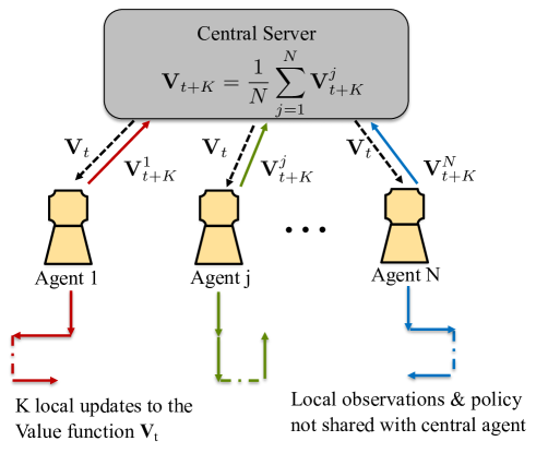
Figure 1: Schematic representation of FRL where ${\rm NewA}$ agents follow a Markovian trajectory and synchronize their parameter every $K$ time steps.

While these questions are well-studied [89, 78, 66, 48] in federated supervised learning, only a few works [86, 74] have attempted to answer them in the context of FRL. However, none of them have established the convergence analysis of FRL algorithms by considering Markovian local trajectories and multiple local updates (see Table 1).

In this paper, we tackle this challenging open problem and answer both the questions listed above. We propose communication-efficient federated versions of on-policy TD, off-policy TD, and $Q$-learning algorithms. In addition, we are the first to establish the convergence bounds for these algorithms in the realistic Markovian setting, showing a linear speedup in the number of agents. Previous works [53, 74] on distributed RL have only shown such a speedup by assuming i.i.d. noise. Moreover, based on experiments, [74] conjectures that linear speedup may be possible under the realistic Markov noise setting, which we establish analytically. The main contributions and organization of the paper are summarized below.

• In the on-policy setting, in Section 4 we propose and analyze federated TD-learning with linear function approximation, where the agents’ goal is to evaluate a common policy using on-policy samples collected in parallel from their environments. The agents only share the updated value function (not data) with the central server, thus saving communication cost. We prove a linear convergence speedup with the number of agents and also characterize the impact of communication frequency on the convergence.

• In the off-policy setting, in Section 5 we propose and analyze the federated off-policy TD-learning and federated $Q$-learning algorithms. Again, we establish a linear speedup in their convergence with respect to the number of agents and characterize the impact of synchronization frequency on the convergence. Since every agent samples data using a private policy and only communicates the updated value or $Q$-function, off-policy FRL helps keep both the data as well as the policy private.

• In Section 6, we propose a general Federated Stochastic Approximation framework with Markovian noise (FedSAM) which subsumes both federated TD-learning and federated $Q$-learning algorithms proposed above. Considering Markovian sampling noise poses a significant challenge in the analysis of this algorithm. The convergence result for FedSAM serves as a workhorse that enables us to analyze both federated TD-learning and federated $Q$-learning. We characterize the convergence of FedSAM with a refined analysis of general stochastic approximation algorithms, fundamentally improving upon prior work.

2 Related Work

Table 1: Comparison of sample complexity results for federated supervised learning (local SGD) and reinforcement learning algorithms. The possible distributed architectures are: 1) Worker-server, with a central server that coordinates with $N$ agents; 2) Decentralized, where each agent directly communicates with its neighboring agents, without a central server; and 3) Shared memory, where each agent modifies a subset of the parameters of a global model held in a shared memory, that is accessible to all agents. [68].

Algorithm	Architecture	References	Local Updates	Markov Noise	Linear Speedup
Local SGD	Worker-server	[39]		✗
Local SGD	Worker-server	[76]		✗
TD(0)	Worker-server	[53]		✗
Stochastic Approximation	Decentralized	[86]	✗		✗
A3C-TD(0)	Shared memory	[74]	✗	✗
A3C-TD(0)	Shared memory	[74]	✗		✗
TD & $Q$-learning	Worker-server	This paper

Single node TD-learning and Q-learning. Most existing RL literature is focused on designing and analyzing algorithms that run at a single computing node. In the on-policy setting, the asymptotic convergence of TD-learning was established in [85, 82, 12], and the finite-sample bounds were studied in [25, 45, 11, 77, 34, 19]. In the off-policy setting, [56, 97] study the asymptotic and [17, 19] characterize the finite time bound of TD-learning. The $Q$-learning algorithm was first proposed in [91]. There has been a long line of work to establish the convergence properties of $Q$-learning. In particular, [84, 36, 9, 13, 12] characterize the asymptotic convergence of $Q$-learning, [5, 7, 87, 17, 19] study the finite-sample convergence bound in the mean-square sense, and [29, 47, 65] study the high-probability convergence bounds of $Q$-learning.

Federated Learning with i.i.d. Noise. When multiple agents are used to expedite sample collection, transferring the samples to a central server for the purpose of training can be costly in applications with high-dimensional data [73] and it may also compromise the agents’ privacy. Federated Learning (FL) is an emerging distributed optimization paradigm [44, 37] that utilizes local computation at the agents to train models, such that only model updates, not data, is shared with the central server. In local Stochastic Gradient Descent (Local SGD or FedAvg) [57, 78], the core algorithm in FL, locally trained models are periodically averaged by the central server in order to achieve consensus among the agents at a reduced communication cost. While the convergence of local SGD has been extensively studied in prior work [39, 76, 66, 42], these works assume i.i.d. noise in the gradients, which is acceptable for SGD but too restrictive for RL algorithms.

Distributed and Multi-agent RL. Some recent works have analyzed distributed and multi-agent RL algorithms in the presence of Markovian noise in various settings such as decentralized stochastic approximation [26, 79, 86, 96], TD learning with linear function approximation [88], and off-policy TD in actor-critic algorithms [23, 24]. However, all these works consider decentralized settings, where the agents communicate with their neighbors after every local update. On the other hand, we consider a federated setting, with each agent performing multiple local updates between successive communication rounds, thereby resulting in communication savings. In [74], a parallel implementation of asynchronous advantage actor-critic (A3C) algorithm (which does not have local updates) has been proposed under both i.i.d. and Markov sampling. However, the authors prove a linear speedup only for the i.i.d. case, and an almost linear speedup is observed experimentally for the Markovian case.

3 Preliminaries: Single Node Setting

We model our RL setting with a Markov Decision Process (MDP) with 5 tuples $(\mathcal{S},\mathcal{A},\mathcal{P},\mathcal{R},\gamma)$, where $\mathcal{S}$ and $\mathcal{A}$ are finite sets of states and actions, $\mathcal{P}$ is the set of transition probabilities, $\mathcal{R}$ is the reward function, and $\gamma\in(0,1)$ denotes the discount factor. At each time step $t$, the system is in some state $S_{t}$, and the agent takes some action $A_{t}$ according to a policy $\pi(\cdot|S_{t})$ in hand, which results in reward $\mathcal{R}(S_{t},A_{t})$ for the agent. In the next time step, the system transitions to a new state $S_{t+1}$ according to the state transition probability $\mathcal{P}(\cdot|S_{t},A_{t})$. This series of states and actions $(S_{t},A_{t})_{t\geq 0}$ constructs a Markov chain, which is the source of the Markovian noise in RL. Throughout this paper we assume that this Markov chain is irreducible and aperiodic (also known as ergodic). It is known that this Markov chain asymptotically converges to a steady state, and we denote its stationary distribution with $\mu^{\pi}$.

To measure the long-term reward achieved by following policy $\pi$, we define the value function

$$V^{\pi}(s) ={\mathbb{E}}\left[\sum_{t=0}^{\infty}\gamma^{t}\mathcal{R}(S_{t},A_{t})|S_{0}=s,A_{t}\sim\pi(\cdot|S_{t})\right].$$ (1)

Equation (1) is the tabular representation of the value function. Sometimes, however, the size of the state space $|\mathcal{S}|$ is large, and storing $V^{\pi}(s)$ for all $s\in\mathcal{S}$ is computationally infeasible. Hence, a low dimensional vector ${\mathbf{v}}^{\pi}\in\mathbb{R}^{d}$, where $d\ll|\mathcal{S}|$, can be used to approximate the value function as $V^{\pi}(s)\approx\phi(s)^{\top}{\mathbf{v}}^{\pi}$ [85]. Here $\phi(s)\in\mathbb{R}^{d}$ is a given feature vector corresponding to the state $s$. Using a low-dimensional vector ${\mathbf{v}}^{\pi}$ to approximate a high-dimensional vector $(V^{\pi}(s))_{s\in\mathcal{S}}$ is referred to as the function approximation paradigm in RL. For each $(s,a)$ pair, we also define the $Q$-function, $Q^{\pi}(s,a)={\mathbb{E}}[\sum_{t=0}^{\infty}\gamma^{t}\mathcal{R}(S_{t},A_{t})|S_{0}=s,A_{0}=a]$, which will be employed in $Q$-learning.

3.1 Temporal Difference Learning

An intermediate goal in RL is to estimate the value function (either $(V^{\pi}(s))_{s\in\mathcal{S}}$ or ${\mathbf{v}}^{\pi}$) corresponding to a particular policy $\pi$ using data collected from the environment. This task is denoted as policy evaluation and one of the commonly-used approaches to accomplish this is Temporal Difference (TD)-learning [80]. TD-learning is an iterative algorithm where the elements of a $d$ (or $|\mathcal{S}|$, in the tabular setting) dimensional vector is updated until it converges to ${\mathbf{v}}^{\pi}$ (or $V^{\pi}$). This evaluated value function can be employed in different RL algorithms such as actor-critic [43]. In the on-policy function approximation setting, the update of the $n$-step TD-learning is as follows

$$\begin{split}\text{Sample}&\quad A_{t+n}\sim\pi(\cdot|S_{t+n}),S_{t+n+1}\sim{\mathcal{P}}(\cdot|S_{t+n},A_{t+n})\\ \text{update}&\quad{\mathbf{v}}_{t+1}={\mathbf{v}_{t}}+\alpha\phi(S_{t})\sum_{l=t}^{t+n-1}\gamma^{l-t}(\mathcal{R}(S_{l},A_{l})+\gamma\phi(S_{l\!+\!1})^{\top}{\mathbf{v}_{t}}\!-\!\phi(S_{l})^{\top}{\mathbf{v}_{t}}),\end{split}$$ (2)

where $\alpha$ is the step size. Note that in this setting, the evaluating policy and the sampling policy coincide. In contrast, in the off-policy setting these two policies can in general differ, and we need to account for this difference while running the algorithm. We will further expand on TD-learning and its variants in Sections 4.1 and 5.1.1.

3.2 Control Problem and $Q$-learning

Assuming some initial distribution $\xi$ on the state space, the average value function corresponding to policy $\pi$ is defined as $V^{\pi}(\xi)={\mathbb{E}}_{s\sim\xi}[V^{\pi}(s)]$. This scalar quantity is a metric of average long-term rewards achieved by the agent, when it starts from distribution $\xi$ and follows policy $\pi$. The ultimate goal of the agent is to obtain an optimal policy $\pi^{*}$ which results in the maximum long-term rewards, i.e. $\pi^{*}\in\operatorname*{arg\,max}_{\pi}V^{\pi}(\xi)$. Throughout the paper, we denote the parameters corresponding to the optimal policy with ^∗, e.g., $V^{\pi^{*}}(\xi)\equiv V^{*}(\xi)$. The task of obtaining the optimal policy in RL is denoted as the control problem.

$Q$-learning [91] is one of the most widely used algorithms in RL to solve the control problem. At each time step $t$, $Q$-learning preserves a $|\mathcal{S}|.|\mathcal{A}|$ dimensional table $Q_{t}$, and updates it table as ${Q}_{t+1}(s,a)={Q}_{t}(S_{t},A_{t})+\alpha(\mathcal{R}(S_{t},A_{t})+\gamma\max_{a}{Q}_{t}(S_{t+1},a)-{Q}_{t}(S_{t},A_{t}))$, if $(s,a)=(S_{t},A_{t})$ and ${Q}_{t+1}(s,a)={Q}_{t}(s,a)$ otherwise. The $|\mathcal{S}||\mathcal{A}|$ elements of the vector $Q_{t}$ are updated iteratively until it converges to $Q^{*}$, corresponding to an optimal policy. Using $Q^{*}$, one can obtain an optimal policy via greedy selection.

3.3 Stochastic Approximation and Finite Sample Bounds

Both TD-learning and $Q$-learning can be seen as variants of stochastic approximation [18, 21, 22, 20, 84]. While generic stochastic approximation algorithms are studied under i.i.d. noise [29, 70, 87, 51, 25], to apply them for studying RL we need to understand stochastic approximation under Markovian noise [84, 65, 77, 19] which is significantly more challenging.

For a generic stochastic approximation (i.i.d. or Markovian noise) with constant step size $\alpha$, parameter vector ${\mathbf{x}}_{T}$, and convergent point ${\mathbf{x}}^{*}$, it can be shown that the algorithm have the following convergence behaviour

$${\mathbb{E}}[\|{\mathbf{x}}_{T}-{\mathbf{x}}^{*}\|^{2}]\leq\mathcal{C}_{1}(1-\mathcal{C}_{0}\alpha)^{T}+\mathcal{C}_{2}\alpha,$$ (3)

where $\mathcal{C}_{0},\mathcal{C}_{1},$ and $\mathcal{C}_{2}$ are some problem dependent positive constants (Look at Appendix A for a discussion on a lower bound on the convergence of general stochastic approximation). The first term is denoted as the bias and the second term is called the variance. According to this bound, ${\mathbf{x}}_{T}$ geometrically converges to a ball around ${\mathbf{x}}^{*}$ with radius proportional to $\mathcal{C}_{2}\alpha$. Notice that we can always reduce the variance term by reducing the step size $\alpha$, but this will lead to slower convergence in the bias term. In particular, in order to get ${\mathbb{E}}[\|{\mathbf{x}}_{T}-{\mathbf{x}}^{*}\|^{2}]\leq\epsilon$, it is easy to see that we need $T\geq\mathcal{O}\left(\frac{\mathcal{C}_{2}}{\epsilon}\log\frac{1}{\epsilon}\right)$ sample complexity. Now suppose the constant $\mathcal{C}_{2}$ is large. In this case, the variance term in the bound in (3) is large, and the sample complexity, which is proportional to $\mathcal{C}_{2}$ will be poor. Notice that by the discussion in Appendix A, this bound is tight and cannot be improved.

This is where the FL can be employed in order to control the variance term by generating more data. For instance, in federated TD-learning, multiple agents work together to evaluate the value function simultaneously. Due to this collaboration, the agents can estimate the true value function with a lower variance. The same holds for estimating $Q^{*}$ in $Q$-learning.

4 Federated On-policy RL

4.1 On-policy TD-learning with linear function approximation

In this section we describe the TD-learning with linear function approximation and online data samples in the single node setting. In this problem, we consider a full rank feature matrix $\Phi\in|\mathcal{S}|\times d$, and we denote $s$-th row of this matrix with $\phi(s),s\in\mathcal{S}$. The goal is to find ${\mathbf{v}}^{\pi}\in\mathbb{R}^{d}$ which solves the following fixed point equation:

$$\Phi{\mathbf{v}}^{\pi}=\Pi_{\Phi}((\mathcal{T}^{\pi})^{n}\Phi{\mathbf{v}}^{\pi}).$$ (4)

In equation (4), $\Pi_{\Phi}(\cdot)$ is the projection with respect to the weighted 2-norm, i.e., $\Pi_{\Phi}({\mathbf{V}})=\operatorname*{arg\,min}_{\mathbf{v}\in\mathbb{R}^{d}}\|\Phi{\mathbf{v}}-{\mathbf{V}}\|_{\pi}$. Here $\|{\mathbf{V}}\|_{\pi}=\sqrt{{\mathbf{V}}^{\top}{\bm{\mu}}^{\pi}{\mathbf{V}}}$ and ${\bm{\mu}}^{\pi}$ is a diagonal matrix with diagonal entries corresponding to $\mu^{\pi}$. In equation (4), $(\mathcal{T}^{\pi})^{n}$ denotes the $n$-step Bellman operator [85]. It is known [85] that equation (4) has a unique solution ${\mathbf{v}}^{\pi}$, and $\Phi{\mathbf{v}}^{\pi}$ is “close” to the true value function $V^{\pi}$. $n$-step TD-learning algorithm, which was shown in (2), is an iterative algorithm to obtain this unique fixed point using samples from the environment. Note that in this algorithm states and actions are sampled over a single trajectory, and hence the noise in updating ${\mathbf{v}}_{t}$ is Markovian. Furthermore, since the policy which samples the actions and the the evaluating policy are both $\pi$, this algorithm is on-policy. As described in [85, 10], the TD-learning algorithm can be studied under the umbrella of linear stochastic approximation with Markovian noise. More recently, the authors in [11, 77] have shown that the update parameter of TD-learning ${\mathbf{v}}_{t}$ converges to ${\mathbf{v}}^{\pi}$ in the form ${\mathbb{E}}[\|{\mathbf{v}}_{t}-{\mathbf{v}}^{\pi}\|^{2}_{2}]\leq\mathcal{O}((1-\mathcal{C}_{0}\alpha)^{t}+\alpha)$. In the next section we show how FL can improve this result.

4.2 Federated TD-learning with linear function approximation

The federated version of on-policy $n$-step TD-learning with linear function approximation is shown in Algorithm 1. In this algorithm we consider ${\rm NewA}$ agents which collaboratively work together to evaluate ${\mathbf{v}}^{\pi}$. For each agent $i,i=1,2,\dots,{\rm NewA}$, we initialize their corresponding parameters ${\mathbf{v}}^{i}_{0}=\mathbf{0}$. Furthermore, each agent $i$ samples its initial state $S_{0}^{i}$ from some given distribution $\xi$. In the next time steps, each agent follows a single Markovian trajectory generated by policy $\pi$, independently from other agents. At each time $t$, the parameter of each agent $i$ is updated using this independently generated trajectory as ${\mathbf{v}}_{t+1}^{i}={\mathbf{v}^{i}_{t}}+\alpha\phi(S_{t}^{i})E_{t,n}^{i}$. Finally, in order to ensure convergence to a global optimum, every $K$ time steps all the agents send their parameters to a central server. The central server evaluates the average of these parameters and returns this average to each of the agents. Each agent then continues their update procedure using this average.

Notice that the averaging step is essential to ensure synchronization among the agents. Smaller $K$ results in more frequent synchronization, and hence better convergence guarantees. However, setting smaller $K$ is equivalent to more number of communications between the single agents and the central server, which incurs higher cost. Hence, an intermediate value for $K$ has to be chosen to strike a balance between the communication cost and the accuracy. At the end, the algorithm samples a time step $\hat{T}\sim q^{c}_{T}$, where

$$q^{c}_{T}(t)=\frac{c^{-t}}{\sum_{t^{\prime}=0}^{T-1}c^{-t^{\prime}}}\quad\text{for}\quad t=0,1,\dots,T-1$$ (5)

and $c>1$ is some constant. Since we have $q^{c}_{T}(t)\geq 0$ and $\sum_{t=0}^{T-1}q^{c}_{T}(t)=1$, it is clear that $q^{c}_{T}(\cdot)$ is a probability distribution over the time interval $[0,T-1]$. In Theorem 4.1 we characterize the convergence of this algorithm as a function of $\alpha$, ${\rm NewA}$, and $K$. Throughout the paper, $\tilde{O}(\cdot)$ ignores the logarithmic terms.

Algorithm 1 Federated $n$-step TD (On-policy, Function Approx.)

1:  Input: Policy $\pi,\xi$

2:  Initialization: ${\mathbf{v}}^{i}_{0}=\mathbf{0}$ and $S_{0}^{i}\sim\xi$ and $\{A_{l}^{i},S_{l+1}^{i}\}\sim\pi$ for $0\leq l\leq n-1$ and all $i$

3:  for $t=0$ to $T-1$ do

4:     for $i=1,\dots,{\rm NewA}$ do

5:        Sample $A_{t+n}^{i}\sim\pi(\cdot|S_{t+n}^{i}),S_{t+n+1}^{i}\sim{\mathcal{P}}(\cdot|S_{t+n}^{i},A_{t+n}^{i})$

6:        $e_{t,l}^{i}\!=\!\mathcal{R}(S_{l}^{i},A_{l}^{i})\!+\!\gamma\phi(S_{l\!+\!1}^{i})^{\top}{\mathbf{v}^{i}_{t}}\!-\!\phi(S_{l}^{i})^{\top}{\mathbf{v}^{i}_{t}}$ for $l=t,\dots,t+n-1$

7:        $E_{t,n}^{i}=\sum_{l=t}^{t+n-1}\gamma^{l-t}e_{t,l}^{i}$

8:        ${\mathbf{v}}_{t+1}^{i}={\mathbf{v}^{i}_{t}}+\alpha\phi(S_{t}^{i})E_{t,n}^{i}$

9:     end for

10:     if $t+1$ mod $K=0$ then

11:        ${\mathbf{v}}^{i}_{t+1}\leftarrow\frac{1}{{\rm NewA}}\sum_{j=1}^{\rm NewA}{\mathbf{v}}^{j}_{t+1},\forall\ i\in[{\rm NewA}]$

12:     end if

13:  end for

14:  Sample $\hat{T}\sim q^{c_{TDL}}_{T}$

15:  Return: $\frac{1}{{\rm NewA}}\sum_{i=1}^{\rm NewA}{\mathbf{v}}^{i}_{\hat{T}}$

Theorem 4.1.

Let ${\mathbf{v}}_{\hat{T}}=\frac{1}{{\rm NewA}}\sum_{i=1}^{\rm NewA}{\mathbf{v}}^{i}_{\hat{T}}$ denote the average of the parameters across agents at the random time $\hat{T}$. For small enough step size $\alpha$, and $T\geq\mathcal{O}(\log\frac{1}{\alpha})$, there exist constant $c_{TDL}\in(0,1)$ (see Section C.1 for precise statement), such that we have

$${\mathbb{E}}[\|{\mathbf{v}}_{\hat{T}}-{\mathbf{v}}^{\pi}\|_{2}^{2}]\leq \mathcal{C}_{1}^{TD_{L}}\frac{1}{\alpha}(1-\alpha\mathcal{C}_{0}^{TD_{L}})^{T}+\mathcal{C}_{2}^{TD_{L}}\frac{\alpha\tau_{\alpha}^{2}}{{\rm NewA}}+\mathcal{C}_{3}^{TD_{L}}(K-1)\alpha^{2}\tau_{\alpha}+\mathcal{C}_{4}^{TD_{L}}\alpha^{3}\tau_{\alpha}^{2},$$

where $\mathcal{C}_{i}^{TD_{L}}$, $i=0,1,2,3,4$ are problem dependent constants, and $\tau_{\alpha}=\mathcal{O}(\log(1/\alpha))$. By choosing $\alpha=\mathcal{O}(\frac{\log({\rm NewA}T)}{T})$ and $K=T/{\rm NewA}$, we achieve ${\mathbb{E}}[\|{\mathbf{v}}_{\hat{T}}-{\mathbf{v}}^{\pi}\|_{2}^{2}]\leq\epsilon$ within $T=\tilde{\mathcal{O}}\left(\frac{1}{{\rm NewA}\epsilon}\right)$ iterations.

For brevity purposes, here we did not show the exact dependence of the constants $\mathcal{C}_{i}^{TD_{L}}$, $i=0,1,2,3$ on the problem dependent constants. For a discussion on the detailed expression look at Section C.1 in the appendix.

Theorem 4.1 shows that federated TD-learning with linear function approximation enjoys a linear speedup with respect to the number of agents. Compared to the convergence bound of general stochastic approximation in (3), the bound in Theorem 4.1 has three differences. Firstly, the variance term which is proportional to the step size $\alpha$ is divided with the number of agents ${\rm NewA}$. This will allow us to control the variance (and hence improve sample complexity) by employing more number of agents. Secondly, we have an extra term which is zero with perfect synchronization $K=1$. Although this term is not divided with ${\rm NewA}$, but it is proportional to $\alpha^{2}$, which is one order higher than the variance term in (3). Finally, the last term is of the order $\tilde{\mathcal{O}}(\alpha^{3})$, which can be handled by choosing small enough step size.

Furthermore, according to the choice of $K$ in Theorem 4.1, after $T$ iterations, the communication cost of federated TD is $T/K={{\rm NewA}}$. However, by employing federated TD-learning in the naive setting where all the agents communicate with the central server at every time step, the communication cost will be $\mathcal{O}(T)$. Hence, we observe that by carefully tuning the hyper parameters of federated TD, we can significantly reduce the communication cost of the overall algorithm, while not loosing performance in terms of the sample complexity.

Finally, federated TD-learning Algorithm 1 preserves the privacy of the agents. In particular, since the single agents only require to share their parameters ${\mathbf{v}}_{t+1}^{i}$, the central server will not be exposed to the state-action-reward trajectory generated by each agent. This can be essential in some applications where privacy is an issue [59, 83]. Examples of such applications include autonomous driving [49, 99], Internet of Things (IoT) [62, 69, 90], and cloud robotics [52, 92].

Remark.

In algorithm 1, the randomness in choosing $\hat{T}$ is independent of all the other randomness in the problem. Hence, in a practical setting, one can sample $\hat{T}$ ahead of time, before running the algorithm, and stop the algorithm at time step $\hat{T}$ and output ${\mathbf{v}}_{\hat{T}}$. By this method, we require only a single data point to be saved, which results in the memory complexity of $\mathcal{O}(1)$ for the algorithm.

5 Federated Off-Policy RL

On-policy TD-learning requires online sampling from the environment, which might be costly (e.g. robotics [33, 46]), high risk (e.g. self-driving cars [95, 55]), or unethical (e.g. in clinical trials [32, 54, 31]). Off-policy training in RL refers to the paradigm where we use data collected by a fixed behaviour policy to run the algorithm. When employed in federated setting, off-policy RL has privacy advantages as well [30, 64, 100]. In particular, suppose each single agent attains a unique sampling policy, and they do not wish to reveal these policies to the central server. In off-policy FL, agents only transmit sampled data, and hence the sampling policies remain private to each agent.

In Section 5.1 we will discuss off-policy TD-learning and in Section 5.2 we will discuss $Q$-learning, which is an off-policy control algorithm. For the off-policy algorithms, we only study the tabular setting. Notice that it has been observed that the combination of off-policy sampling and function approximation in RL (also known as deadly triad [81]) can result in instability or even divergence [2]. Recently there has been some work to overcome deadly triad [16]. Extension of our work to function approximation in the off-policy setting is a future research direction.

5.1 Federated Off-Policy TD-learning

In the following, we first discuss single-node off-policy TD-learning, and then we generalize it to the federated setting.

5.1.1 Off-policy TD-learning

In off-policy TD-learning the goal is to evaluate the value function ${\mathbf{V}}^{\pi}=(V^{\pi}(s))_{s\in\mathcal{S}}$ corresponding to the policy $\pi$ using data sampled from some fixed behaviour policy $\pi_{b}$. In this setting, the evaluating policy $\pi$ and the sampling policy $\pi_{b}$ can be arbitrarily different, and we need to account for this difference while performing the evaluation. Although $\pi$ and $\pi_{b}$ can be different, notice that the value function ${\mathbf{V}}^{\pi}$ does not depend on $\pi_{b}$. In order to account for this difference, we introduce the notion of importance sampling as $\mathfrak{I}^{b}(s,a)=\frac{\pi(a|s)}{\pi^{b}(a|s)}$ which is employed in the off-policy TD-learning.

Recently, several works studied the finite-time convergence of off-policy TD-learning. In particular, the authors in [40, 19, 18, 20] show that, similar to on-policy TD, off-policy TD-learning can be studied under the umbrella of stochastic approximation. Hence, this algorithm enjoys similar convergence behaviour as (3).

5.1.2 Federated off-policy TD-learning

The federated version of $n$-step off-policy TD-learning is shown in Algorithm 2. In this algorithm, each agent $i$ attains a unique (and private) sampling policy $\pi^{i}$ and follows an independent trajectory generated by this policy. Furthermore, at each time step $t$, each agent $i$ attains a $|\mathcal{S}|$-dimensional vector ${\mathbf{V}}^{i}_{t}$ and updates this vector using the samples generated by $\pi^{i}$. In order to account for the off-policy sampling, each agent utilizes $\mathfrak{I}^{(i)}(S^{i},A^{i})=\frac{\pi(A^{i}|S^{i})}{\pi^{i}(A^{i}|S^{i})}$ in the update of their algorithm. We further define $\mathfrak{I}_{\max}=\max_{s,a,i}\mathfrak{I}^{(i)}(s,a)$, which is a measure of discrepancy between the evaluating policy $\pi$ and sampling policy $\pi^{i}$ of all the agents.

In order to ensure synchronization, all the agents transmit their parameter vectors to the central server every $K$ time steps. The central server returns the average of these vectors to each agent and each agent follows this averaged vector afterwards. Notice that in federated off-policy TD-learning Algorithm 2, each agent share neither their sampled trajectory of state-action-rewards, nor their sampling policy with the central server. This provides two levels of privacy for the single agents. At the end, the algorithm samples a time step $\hat{T}\sim q_{T}^{c_{TD}}$, where the distribution $q_{T}^{c}$ is defined in (5) and $c_{TD}=1-\frac{\alpha{\varphi}_{TD}}{2}$, where ${\varphi}_{TD}=1-\frac{0.5e^{1/4}(2-\mu_{\min}(1-\gamma^{n+1}))}{\sqrt{\sqrt{e}-1+\left(\frac{2-\mu_{\min}(1-\gamma^{n+1})}{2-2\mu_{\min}(1-\gamma^{n+1})}\right)^{2}}}$. Here, we denote $\mu_{\min}=\min_{s,i}\mu^{\pi^{i}}(s)$. The constant $c_{TD}$ is carefully chosen to ensure the convergence of Algorithm 2. Furthermore, for small enough step size $\alpha$, it can be shown that $0<c_{TD}<1$.

Algorithm 2 Federated $n$-step TD (Off-policy Tabular Setting)

1:  Input: Policy $\pi,\xi$

2:  Initialization: ${\mathbf{V}}_{0}^{i}=\mathbf{0}$ and $S_{0}^{i}\sim\xi$ and $\{A_{l}^{i},S_{l+1}^{i}\}\sim\pi^{i}$ for $0\leq l\leq n-1$ and all $i$

3:  for $t=0$ to $T-1$ do

4:     for $i=1,\dots,{\rm NewA}$ do

5:        Sample $A_{t+n}^{i}\sim\pi^{i}(\cdot|S_{t+n}^{i}),S_{t+n+1}^{i}\sim{\mathcal{P}}(\cdot|S_{t+n}^{i},A_{t+n}^{i})$

6:        $e_{t,l}^{i}=\mathcal{R}(S_{l}^{i},A_{l}^{i})\!+\!\gamma{\mathbf{V}}_{t}^{i}(S_{l+1}^{i})-{\mathbf{V}}_{t}^{i}(S_{l}^{i})$

7:        Update ${\mathbf{V}}_{t+1}^{i}(s)={\mathbf{V}}_{t}^{i}(s)+\alpha\sum_{l=t}^{t+n-1}\gamma^{l-t}\left[\Pi_{j=t}^{l}\mathfrak{I}^{(i)}(S^{i}_{j},A^{i}_{j})\right]e_{t,l}^{i}$ if $s=S_{t}^{i}$ and ${\mathbf{V}}_{t+1}^{i}(s)={\mathbf{V}}_{t}^{i}(s)$ otherwise.

8:     end for

9:     if $t+1$ mod $K=0$ then

10:        ${\mathbf{V}}_{t+1}^{i}\leftarrow\frac{1}{{\rm NewA}}\sum_{j=1}^{\rm NewA}{\mathbf{V}}^{j}_{t+1},\forall\ i\in[{\rm NewA}]$

11:     end if

12:  end for

13:  Sample $\hat{T}\sim q_{T}^{c_{TD}}$

14:  Return: $\frac{1}{{\rm NewA}}\sum_{i=1}^{\rm NewA}{\mathbf{V}}^{i}_{\hat{T}}$

Theorem 5.1 states the convergence of this Algorithm.

Theorem 5.1.

Consider the federated $n$-step off-policy TD-learning Algorithm 2. Denote ${\mathbf{V}}_{\hat{T}}=\frac{1}{{\rm NewA}}\sum_{i=1}^{\rm NewA}{\mathbf{V}}_{\hat{T}}^{i}$. For small enough step size $\alpha$ and large enough $T$, we have

$${\mathbb{E}}[\|{\mathbf{V}}_{\hat{T}}-{\mathbf{V}}^{\pi}\|_{\infty}^{2}]\leq \mathcal{C}_{1}^{TD_{T}}\frac{1}{\alpha}c_{TD}^{T}+\mathcal{C}_{2}^{TD_{T}}\frac{\alpha\tau_{\alpha}^{2}}{{\rm NewA}}+\mathcal{C}_{3}^{TD_{T}}(K-1)\alpha^{2}\tau_{\alpha},$$

where $\mathcal{C}_{1}^{TD_{T}}=\bar{\mathcal{C}}_{1}^{TD_{T}}.\frac{\mathfrak{I}_{\max}^{4n-2}}{\mu_{\min}(1-\gamma)^{3}}$, $\mathcal{C}_{2}^{TD_{T}}=\bar{\mathcal{C}}_{2}^{TD_{T}}.\frac{\mathfrak{I}_{\max}^{3n-1}|\mathcal{S}|\log^{2}(|\mathcal{S}|)}{\mu_{\min}^{2}(1-\gamma)^{4}}$, $\mathcal{C}_{3}^{TD_{T}}=\bar{\mathcal{C}}_{3}^{TD_{T}}.\frac{\mathfrak{I}_{\max}^{7n-3}|\mathcal{S}|^{2}\log^{2}(|\mathcal{S}|)}{\mu_{\min}^{4}(1-\gamma)^{8}}$, and $\bar{\mathcal{C}}_{i}^{TD_{T}}$, $i=1,2,3$ are universal problem independent constants. In addition, choosing $\alpha=\frac{8\log({\rm NewA}T)}{T{\varphi}_{TD}}$ and $K=T/{\rm NewA}$, we have ${\mathbb{E}}[\|{\mathbf{V}}_{\hat{T}}-{\mathbf{V}}^{\pi}\|_{\infty}^{2}]\leq\epsilon$ after $T=\tilde{\mathcal{O}}\left(\frac{1}{{\rm NewA}\epsilon}.\frac{\mathfrak{I}_{\max}^{7n-3}|\mathcal{S}|^{2}\log^{2}(|\mathcal{S}|)}{\mu_{\min}^{5}(1-\gamma)^{9}}\right)$ iterations.

The proof is given in Section C.2 in the appendix.

Note that similar to on-policy TD-learning Algorithm 1, off-policy TD-learning also enjoys a linear speedup while maintaining a low communication cost. In addition, this algorithm preserves the privacy of the agents by holding both the data and the sampling policy private.

5.2 Federated $Q$-learning

So far we have discussed policy evaluation problem with on and off-policy samples. Next we aim at solving the control problem by employing the celebrated $Q$-learning algorithm [91, 84]. In the next section we will explain the $Q$-learning algorithm. Further, in Section 5.2.2 we will provide a federated version of $Q$-learning along with its convergence result.

5.2.1 $Q$-learning

The goal of $Q$-learning is to evaluate $Q^{*}$, which is the unique $Q$-function corresponding to the optimal policy. Knowing $Q^{*}$, one can obtain an optimal policy through a greedy selection [63], and hence resolve the control problem.

Suppose $\{S_{t},A_{t}\}_{t\geq 0}$ is generated by a fixed behaviour policy $\pi_{b}$. At each time step $t$, $Q$-learning preserves a $|\mathcal{S}|.|\mathcal{A}|$ table $Q_{t}$ and updates the elements of this table as shown in Section 3.2. By assuming $\pi_{b}$ to be an ergodic policy, the asymptotic convergence of $Q_{t}$ to $Q^{*}$ has been established in [9]. Furthermore, it can be shown that $Q$-learning is a special case of stochastic approximation and enjoys a convergence bound similar to (3) [6, 47, 65, 19].

Two points worth mentioning about the $Q$-learning algorithm. Firstly, $Q$-learning is an off-policy algorithm in the sense that only samples from a fixed ergodic policy is needed to perform the algorithm. Secondly, as opposed to the TD-learning, the update of the $Q$-learning is non-linear. This imposes a sharp contrast between the analysis of $Q$-learning and TD-learning [22].

5.2.2 Federated $Q$-learning

Algorithm 3 provides the federated version of $Q$-learning. We characterize its convergence in the following theorem.

Algorithm 3 Federated $Q$-learning

1:  Input: Sampling policy $\pi^{i}_{b}$ for $i=1,2,\dots,{\rm NewA}$, initial distribution $\xi$

2:  Initialization: ${Q}^{i}_{0}=\mathbf{0}$ and $S_{0}^{i}\sim\xi$ for all $i$

3:  for $t=0$ to $T-1$ do

4:     for $i=1,\dots,{\rm NewA}$ do

5:        Sample $A_{t}^{i}\sim\pi_{b}^{i}(\cdot|S_{t}^{i}),S_{t+1}^{i}\sim{\mathcal{P}}(\cdot|S_{t}^{i},A_{t}^{i})$

6:         Update ${Q}^{i}_{t+1}(s,a)={Q}^{i}_{t}(S^{i}_{t},A^{i}_{t})+$ $\alpha\left[\mathcal{R}(S^{i}_{t},A^{i}_{t})+\gamma\max_{a}{Q}^{i}_{t}(S^{i}_{t+1},a)-{Q}^{i}_{t}(S^{i}_{t},A^{i}_{t})\right]$, if $(s,a)=(S^{i}_{t},A^{i}_{t})$ and ${Q}^{i}_{t+1}(s,a)={Q}^{i}_{t}(s,a)$ otherwise.

7:     end for

8:     if $t+1$ mod $K=0$ then

9:        $Q^{i}_{t+1}\leftarrow\frac{1}{{\rm NewA}}\sum_{j=1}^{\rm NewA}Q^{j}_{t+1},\forall\ i\in[{\rm NewA}]$

10:     end if

11:  end for

12:  Sample: $\hat{T}\sim q_{T}^{c_{Q}}$

13:  Return: $\frac{1}{{\rm NewA}}\sum_{i=1}^{\rm NewA}Q^{i}_{\hat{T}}$

Theorem 5.2.

Consider the federated $Q$-learning Algorithm 3 with $c_{Q}=1-\frac{\alpha{\varphi}_{Q}}{2}\in(0,1)$, where ${\varphi}_{Q}=1-\frac{0.5e^{1/4}(2-\mu_{\min}(1-\gamma))}{\sqrt{\sqrt{e}-1+\left(\frac{2-\mu_{\min}(1-\gamma)}{2-2\mu_{\min}(1-\gamma)}\right)^{2}}}$ and we denote $\mu_{\min}=\min_{s,a,i}\mu^{\pi^{i}}(s)\pi^{i}(a|s)$. Denote ${Q}_{\hat{T}}=\frac{1}{{\rm NewA}}\sum_{i=1}^{\rm NewA}{Q}_{\hat{T}}^{i}$. For small enough step size $\alpha$ and large enough $T$, we have

$${\mathbb{E}}[\|Q_{\hat{T}}-Q^{*}\|_{\infty}^{2}]\leq\mathcal{C}_{1}^{Q}\frac{1}{\alpha}c_{Q}^{T}+\mathcal{C}_{2}^{Q}\frac{\alpha\tau_{\alpha}^{2}}{{\rm NewA}}+\mathcal{C}_{3}^{Q}(K-1)\alpha^{2}\tau_{\alpha},$$

where $\mathcal{C}_{1}^{Q}=\bar{\mathcal{C}}_{1}^{Q}.\frac{1}{\mu_{\min}(1-\gamma)^{3}}$, $\mathcal{C}_{2}^{Q}=\bar{\mathcal{C}}_{2}^{Q}.\frac{|\mathcal{S}|\log^{2}(|\mathcal{S}|)}{\mu_{\min}^{2}(1-\gamma)^{4}}$, $\mathcal{C}_{3}^{Q}=\bar{\mathcal{C}}_{3}^{Q}.\frac{|\mathcal{S}|^{2}\log^{2}(|\mathcal{S}|)}{\mu_{\min}^{4}(1-\gamma)^{8}}$, and $\bar{\mathcal{C}}_{i}^{Q}$, $i=1,2,3$ are universal problem independent constants. In addition, choosing $\alpha=\frac{8\log({\rm NewA}T)}{T{\varphi}_{Q}}$ and $K=T/{\rm NewA}$, we have ${\mathbb{E}}[\|Q_{\hat{T}}-Q^{*}\|_{\infty}^{2}]\leq\epsilon$ within $T=\tilde{\mathcal{O}}\left(\frac{1}{{\rm NewA}\epsilon}.\frac{|\mathcal{S}|^{2}\log^{2}(|\mathcal{S}|)}{\mu_{\min}^{5}(1-\gamma)^{9}}\right)$ iterations.

According to Theorem 5.2, federated $Q$-learning Algorithm 3, similar to federated off-policy TD-learning, enjoys linear speedup, communication efficiency as well as privacy guarantees. We would like to emphasize that the update of $Q$-learning is non-linear. Hence the result of Theorem 5.2 cannot be derived from Theorems 4.1 and 5.1.

6 Generalized Federated Stochastic Approximation

In this section we study the convergence of a general federated stochastic approximation for contractive operators, FedSAM, which is presented in Algorithm 4. In this algorithm there are ${\rm NewA}$ agents $i=1,2,\dots,{\rm NewA}$. At each time step $t\geq 0$, each agent $i$ maintains the parameter ${\bm{\theta}^{i}_{t}}\in\mathbb{R}^{d}$. At time $t=0$, all agents initialize their parameters with ${\bm{\theta}}_{0}^{i}={\bm{\theta}}_{0}$. Next, at time $t\geq 0$, each agent $i$ updates its parameter as ${\bm{\theta}}^{i}_{t+1}={\bm{\theta}^{i}_{t}}+\alpha\left({\mathbf{G}^{i}}({\bm{\theta}^{i}_{t}},{\mathbf{y}^{i}_{t}})-{\bm{\theta}^{i}_{t}}+\mathbf{b}^{i}({\mathbf{y}^{i}_{t}})\right)$. Here $\alpha$ denotes the step size, and ${\mathbf{y}^{i}_{t}}$ is a noise which is Markovian along the time $t$, but is independent across the agents $i$. This notion is defined more concretely in Assumption 6.4. We note that functions ${\mathbf{G}^{i}}(\cdot,\cdot)$ and $\mathbf{b}^{i}(\cdot)$ are allowed to be dependent on the agent $i$. This allows us to employ the convergence bound of FedSAM in order to derive the convergence bound of off-policy TD-learning with different behaviour policies across agents. In order to avoid divergence, every $K$ time steps we synchronize the parameters of all the agents as ${\bm{\theta}^{i}_{t}}\leftarrow{\bm{\theta}_{t}}\triangleq\frac{1}{{\rm NewA}}\sum_{j=1}^{\rm NewA}{\bm{\theta}}_{t}^{j},$ for all $i\in[{\rm NewA}]$. Note that although smaller $K$ corresponds to more frequent synchronization and hence more “accurate” updates, at the same time it results in a higher communication cost, which is not desirable. Hence, in order to determine the optimal choice of synchronization period, it is essential to characterize the dependence of the convergence on $K$. This is one of the results which we will derive in Theorem B.1. Finally, the algorithm samples $\hat{T}\sim q_{T}^{c}$, where $q^{c}_{T}(t)=\frac{c^{-t}}{\sum_{t^{\prime}=0}^{T-1}c^{-t^{\prime}}}$ and outputs ${\bm{\theta}}_{\hat{T}}$. This sampling scheme is essential for the convergence of overall algorithm. We further make some assumptions regarding the underlying process.

Algorithm 4 Federated Stochastic Approximation with Markovian Noise (FedSAM)

1:  Input: $c_{FSAM},T,{\bm{\theta}}_{0},K,\alpha$

2:  ${\bm{\theta}}^{i}_{0}={\bm{\theta}}_{0}$ for all $i=1,\dots,{\rm NewA}$.

3:  for $t=0$ to $T-1$ do

4:     ${\bm{\theta}}^{i}_{t+1}={\bm{\theta}^{i}_{t}}+\alpha\left({\mathbf{G}^{i}}({\bm{\theta}^{i}_{t}},{\mathbf{y}^{i}_{t}})-{\bm{\theta}^{i}_{t}}+\mathbf{b}^{i}({\mathbf{y}^{i}_{t}})\right),\forall\ i\in[{\rm NewA}]$

5:     if $t+1$ mod $K=0$ then

6:        ${\bm{\theta}}^{i}_{t+1}={\bm{\theta}}_{t+1}\triangleq\frac{1}{{\rm NewA}}\sum_{j=1}^{\rm NewA}{\bm{\theta}}^{j}_{t+1},\forall\ i\in[{\rm NewA}]$

7:     end if

8:  end for

9:  Sample $\hat{T}\sim q_{T}^{c_{FSAM}}(\cdot)$.

10:  Return: $\frac{1}{{\rm NewA}}\sum_{i=1}^{\rm NewA}{\bm{\theta}}^{i}_{\hat{T}}$

First, we assume that the expectation of ${\mathbf{G}^{i}}({\bm{\theta}},{\mathbf{y}}_{t}^{i})$ geometrically converges to some function ${\bar{\mathbf{G}}}^{i}({\bm{\theta}})$ and the expectation of $\mathbf{b}^{i}({\mathbf{y}}_{t}^{i})$ geometrically converges to $\mathbf{0}$. In particular, we have the following assumption.

Assumption 6.1.

For every agent $i$, there exist a function ${\bar{\mathbf{G}}}^{i}({\bm{\theta}})$ such that we have

$$\lim_{t\to\infty}{\mathbb{E}}[{\mathbf{G}^{i}}({\bm{\theta}},{\mathbf{y}}_{t}^{i})] ={\bar{\mathbf{G}}}^{i}({\bm{\theta}})$$

$$\lim_{t\to\infty}{\mathbb{E}}[\mathbf{b}^{i}({\mathbf{y}}_{t}^{i})] =\mathbf{0}.$$ (6)

Furthermore, there exists $m_{1},m_{2}\geq 0$ and $\rho\in[0,1)$, such that for every $i=1,2,\dots,{\rm NewA}$,

$$\|{\bar{\mathbf{G}}}^{i}({\bm{\theta}})-{\mathbb{E}}[{\mathbf{G}^{i}}({\bm{\theta}},{\mathbf{y}}_{t}^{i})]\|_{c} \leq m_{1}\|{\bm{\theta}}\|_{c}\rho^{t}$$ (7)

$$\|{\mathbb{E}}[\mathbf{b}^{i}({\mathbf{y}}_{t}^{i})]\|_{c} \leq m_{2}\rho^{t},$$

where $\|\cdot\|_{c}$ is a given norm.

Next, we assume a contraction property on the expected operator ${\bar{\mathbf{G}}}^{i}({\bm{\theta}})$.

Assumption 6.2.

We assume all expected operators ${\bar{\mathbf{G}}}^{i}({\bm{\theta}})$ are contraction mappings with respect to $\|\cdot\|_{c}$ with contraction factor $\gamma_{c}\in(0,1)$. That is, for all $i=1,2,\dots,{\rm NewA}$,

$$\|{\bar{\mathbf{G}}}^{i}({\bm{\theta}}_{1})-{\bar{\mathbf{G}}}^{i}({\bm{\theta}}_{2})\|_{c}\leq\gamma_{c}\|{\bm{\theta}}_{1}-{\bm{\theta}}_{2}\|_{c},~{}~{}\forall\ {\bm{\theta}}_{1},{\bm{\theta}}_{2}\in\mathbb{R}^{d}.$$

Next, we consider some Lipschitz and boundedness properties on ${\mathbf{G}^{i}}(\cdot,\cdot)$ and $\mathbf{b}^{i}(\cdot)$.

Assumption 6.3.

For all $i=1,\dots,{\rm NewA}$, there exist constants $A_{1}$, $A_{2}$ and $B$ such that

1. $\|{\mathbf{G}^{i}}({\bm{\theta}}_{1},{\mathbf{y}^{i}})-{\mathbf{G}^{i}}({\bm{\theta}}_{2},{\mathbf{y}^{i}})\|_{c}\leq A_{1}\|{\bm{\theta}}_{1}-{\bm{\theta}}_{2}\|_{c}$, for all ${\bm{\theta}}_{1},{\bm{\theta}}_{2},{\mathbf{y}^{i}}$.

2. $\|{\mathbf{G}^{i}}({\bm{\theta}},{\mathbf{y}^{i}})\|_{c}\leq A_{2}\|{\bm{\theta}}\|_{c}$ for all ${\bm{\theta}},{\mathbf{y}^{i}}$.

3. $\|\mathbf{b}^{i}({\mathbf{y}}^{i})\|_{c}\leq B$ for all ${\mathbf{y}^{i}}$.

Remark.

By Assumption 6.2 and due to the Banach fixed point theorem, ${\bar{\mathbf{G}}^{i}}(\cdot)$ has a unique fixed point for all $i=1,2,\dots,{\rm NewA}$. Furthermore, by Assumption 6.3, we have ${\mathbf{G}^{i}}(\mathbf{0},{\mathbf{y}})=\mathbf{0}$. Hence the point $\mathbf{0}$ is the unique fixed point of ${\bar{\mathbf{G}}^{i}}(\cdot)$.

Finally, we impose an assumption on the random data ${\mathbf{y}^{i}_{t}}$.

Assumption 6.4.

We assume that the Markovian noise ${\mathbf{y}^{i}_{t}}$ (Markovian with respect to time $t$) is independent across agents $i$. In other words, for all measurable functions $f(\cdot)$ and $g(\cdot)$, we assume the following

$${\mathbb{E}}_{t-r}[f({\mathbf{y}}_{t}^{i})\times g({\mathbf{y}}_{t}^{j})]={\mathbb{E}}_{t-r}[f({\mathbf{y}}_{t}^{i})]\times{\mathbb{E}}_{t-r}[g({\mathbf{y}}_{t}^{j})],$$

for all $r\leq t,i\neq j$.

Theorem 6.1 states the convergence of Algorithm 4.

Theorem 6.1.

Consider the federated stochastic approximation Algorithm 4 with $c_{FSAM}=1-\frac{\alpha{\varphi}_{2}}{2}\in(0,1)$ (${\varphi}_{2}$ is defined in Equation (14) in the appendix), and synchronization frequency $K$. Denote ${\bm{\theta}_{t}}=\frac{1}{{\rm NewA}}\sum_{i=1}^{\rm NewA}{\bm{\theta}^{i}_{t}}$, and consider ${\bm{\theta}}_{\hat{T}}$ as the output of this algorithm after $T$ iterations. Assume $\tau_{\alpha}=\lceil 2\log_{\rho}\frac{1}{\alpha}\rceil$. For $T\geq\max\{K+\tau_{\alpha},2\tau_{\alpha}\}$ and small enough step size $\alpha$, we have

$${\mathbb{E}}[\|{\bm{\theta}}_{\hat{T}}\|^{2}_{c}]\leq \mathcal{C}_{1}\frac{1}{\alpha}c_{FSAM}^{T-2\tau_{\alpha}+1}+\mathcal{C}_{2}\frac{\alpha\tau_{\alpha}^{2}}{{\rm NewA}}+\mathcal{C}_{3}(K-1)\alpha^{2}\tau_{\alpha}+\mathcal{C}_{4}\alpha^{3}\tau_{\alpha}^{2},$$ (8)

where $\mathcal{C}_{i}$, $i=1,2,3,4$ are some constants which are specified precisely in Appendix B, and are independent of $K,\alpha,{\rm NewA}$. Choosing $\alpha=\frac{8\log({\rm NewA}T)}{T{\varphi}_{2}}$ and $K=T/{\rm NewA}$, we get $T=\tilde{\mathcal{O}}\left(\frac{1}{{\rm NewA}\epsilon}\right)$ sample complexity for achieving ${\mathbb{E}}[\|{\bm{\theta}}_{\hat{T}}\|^{2}_{c}]\leq\epsilon$.

Theorem 6.1 establishes the convergence of ${\bm{\theta}}_{\hat{T}}$ to zero in the expected mean-squared sense. The first term in (8) converges geometrically to zero as $T$ grows. The second term is proportional to $\alpha$ similar as (3). However, the number of agents ${\rm NewA}$ in the denominator ensures linear speedup, meaning that for small enough $\alpha$ (such that $\alpha/{\rm NewA}$ is the dominant term), the sample complexity of each individual agent, relative to a centralized system, is reduced by a factor of ${\rm NewA}$. The third term has quadratic dependence on $\alpha$, and is zero when we have perfect synchronization, i.e. $K=1$. The last term is proportional to $\alpha^{3}$, and has the weakest dependency on the step size $\alpha$. For $K>1$ we can merge the last two terms by upper bounding $\alpha^{3}\leq\alpha^{2}$. The current upper bound, however, is tighter since with $K=1$ (i.e. perfect synchronization) we have no term in the order $\alpha^{2}$. Note that similar bounds (sans the last $\alpha^{3}$ term) have been established for the simpler i.i.d. noise case in the federated setting [39, 42]. Consequently, we achieve the same sample complexity results for the more general federated setting with Markov noise.

Remark.

The bound in Theorem 6.1 holds only after $T>\max\{K+\tau_{\alpha},2\tau_{\alpha}\}$ and for all synchronization periods $K\geq 1$. At $K=1$ the third term in the bound goes away, and we will be left only with the first order term, which is linearly decreasing with respect to the number of agents ${\rm NewA}$, and the third order term $\tilde{\mathcal{O}}(\alpha^{3})$. The last term, however, is not tight and can be further improved to be of the order $\mathcal{O}(\alpha^{j}),j>3$. However, for that we need to assume larger $\tau_{\alpha}$, which means the bound only hold after a longer waiting time. In particular, by choosing $\tau_{\alpha}=\lceil r\log_{\rho}\alpha\rceil$, we can get $\tilde{\mathcal{O}}(\alpha^{2r-1})$ for the last term (see the proof of Lemma B.2).

7 Conclusion

In this paper we studied convergence of federated reinforcement learning algorithms, where ${\rm NewA}$ agents aim at completing a common task collaboratively. We proposed Federated TD-learning in both on-policy and off-policy settings, as well as federated $Q$-learning. In all these algorithms, each agent independently follows a Markovian trajectory of state-action-rewards, and update their parameters independently. Furthermore, in order to ensure convergence, the agents synchronize their parameters every $K$ number of iterations.

For all the aforementioned algorithms, we have shown that by choosing small enough step size, and by carefully choosing the communication period $K$, we can boost the overall convergence ${\rm NewA}$ times, while keeping the communication cost to be constant. Finally, we studied FedSAM, which is a general federated stochastic approximation algorithm with Markovian noise, and we established a linear speedup in the convergence of this algorithm.

In our algorithms, evaluation of the sampling distribution of the output time instance $\hat{T}$ requires knowledge of the stationary distribution. An interesting future research direction is to redesign the algorithm to perform without requiring such knowledge. Improving the total communication cost as a function of the number of agents ${\rm NewA}$ is another interesting future direction. In addition, establishing a tighter bound with respect to the constants of the problem can be another direction of interest.

Appendices

The appendices are organized as follows. In section A we discuss the lower bound on the convergence of general stochastic approximation. In Section B we derive the convergence bound of FedSAM algorithm. Next, we employ the results in Section B to derive the convergence bounds of federated TD-learning in Section C and federated $Q$-learning in Section D.

Appendix A Lower Bound on the Convergence of General Stochastic Approximation

In this section we discuss the convergence of general stochastic approximation. In this discussion we provide a simple stochastic approximation with iid noise which can give insight into the general convergence bound in (3). In particular, we show that the convergence bound in (3) is tight and cannot be improved.

Consider a one dimensional random variable $X$ with zero mean ${\mathbb{E}}[X]=0$ and bounded variance ${\mathbb{E}}[X^{2}]=\sigma^{2}$. Consider the following update

$$x_{t+1}=x_{t}+\alpha(X_{t}-x_{t}),\quad t\geq 0,$$ (9)

where we start with some fixed deterministic $x_{0}$ and $X_{t}$ is a an iid sample of the random variable $X$. It is easy to see that the update (9) is a special case of the update of the general stochastic approximation with the fixed point $x^{*}=0$.

By expanding the update (9), we have

$$x_{t}=(1-\alpha)^{t}x_{0}+\alpha\sum_{k=0}^{t-1}(1-\alpha)^{t-k-1}X_{k}.$$

Hence, we have

$$x_{t}^{2}=(1-\alpha)^{2t}x_{0}^{2}+\left(\alpha\sum_{k=0}^{t-1}(1-\alpha)^{t-k-1}X_{k}\right)^{2}+2\alpha(1-\alpha)^{t}x_{0}\sum_{k=0}^{t-1}(1-\alpha)^{t-k-1}X_{k}.$$

Taking expectation on both sides, and using the zero mean property of $X_{k}$, we have

$${\mathbb{E}}[x_{t}^{2}]= (1-\alpha)^{2t}x_{0}^{2}+\alpha^{2}{\mathbb{E}}\left(\sum_{k=0}^{t-1}(1-\alpha)^{t-k-1}X_{k}\right)^{2}$$

$$= (1-\alpha)^{2t}x_{0}^{2}+\alpha^{2}{\mathbb{E}}\left(\sum_{k=0}^{t-1}(1-\alpha)^{2(t-k-1)}X_{k}^{2}+\sum_{k,k^{\prime}=0,k\neq k^{\prime}}^{t-1}(1-\alpha)^{2t-k-k^{\prime}-2}X_{k}X_{k}^{\prime}\right)$$

$$= (1-\alpha)^{2t}x_{0}^{2}+\alpha^{2}\left(\sum_{k=0}^{t-1}(1-\alpha)^{2(t-k-1)}\sigma^{2}+\sum_{k,k^{\prime}=0,k\neq k^{\prime}}^{t-1}(1-\alpha)^{2t-k-k^{\prime}-2}{\mathbb{E}}[X_{k}]{\mathbb{E}}[X_{k}^{\prime}]\right)$$ (iid property)

$$= (1-\alpha)^{2t}x_{0}^{2}+\alpha^{2}\left(\sum_{k=0}^{t-1}(1-\alpha)^{2(t-k-1)}\sigma^{2}\right)$$ (zero mean)

$$= (1-\alpha)^{2t}x_{0}^{2}+\alpha^{2}\sigma^{2}\frac{1-(1-\alpha)^{2t}}{1-(1-\alpha)^{2}}$$

$$= x_{0}^{2}(1-\alpha)^{2t}+\sigma^{2}\frac{1-(1-\alpha)^{2t}}{2-\alpha}\alpha$$

$$= \underbrace{(x_{0}^{2}-\frac{\alpha\sigma^{2}}{2-\alpha})(1-\alpha)^{2t}}_{T_{1}:\text{bias}}+\underbrace{\frac{\sigma^{2}}{2-\alpha}\alpha}_{T_{2}:\text{variance}}.$$ (10)

It is clear that (10) has the same form as the bound in (3) with $T_{1}$ as the geometric term which converges to zero as $t\rightarrow\infty$, and $T_{2}$ term proportional to the step size $\alpha$. In addition, note that in the above derivation, we did not use any inequality, and hence the bounds in (10) as well as (3) are tight.

Appendix B Analysis of Federated Stochastic Approximation

First, we restate Theorem 6.1 with explicit expressions of the different constants.

Theorem B.1.

Consider the FedSAM Algorithm 4 with $c_{FSAM}=1-\frac{\alpha{\varphi}_{2}}{2}$ (${\varphi}_{2}$ is defined in (14)), and suppose Assumptions 6.1, 6.2, 6.3, 6.4 are satisfied. Consider small enough step size $\alpha$ which satisfies the assumptions in (21), (23), (32), (35). Furthermore, denote $\tau_{\alpha}=\lceil 2\log_{\rho}\alpha\rceil$, and take large enough $T$ such that $T>\max\{K+\tau_{\alpha},2\tau_{\alpha}\}$. Then, the output of the FedSAM Algorithm 4, ${\bm{\theta}}_{\hat{T}}\triangleq\frac{1}{{\rm NewA}}\sum_{i=1}^{\rm NewA}{\bm{\theta}}_{\hat{T}}^{i}$, satisfies

$${\mathbb{E}}[\|{\bm{\theta}}_{\hat{T}}\|_{c}^{2}]\leq\mathcal{C}_{1}\frac{1}{\alpha}\left(1-\frac{\alpha{\varphi}_{2}}{2}\right)^{T-2\tau_{\alpha}+1}+\mathcal{C}_{2}\frac{\alpha\tau_{\alpha}^{2}}{{\rm NewA}}+\mathcal{C}_{3}(K-1)\alpha^{2}\tau_{\alpha}+\mathcal{C}_{4}\alpha^{3}\tau_{\alpha}^{2},$$ (11)

where $\mathcal{C}_{1}=16u_{cm}^{2}M_{0}(\log_{\rho}\frac{1}{e}+\frac{1}{{\varphi}_{2}})$, $M_{0}=\frac{1}{l_{cm}^{2}}\left(\frac{1}{C_{1}^{2}}\left(B+(A_{2}+1)\left(\|{\bm{\theta}}_{0}\|_{c}+\frac{B}{2C_{1}}\right)\right)^{2}+\|{\bm{\theta}}_{0}\|_{c}^{2}\right)$, $\mathcal{C}_{2}=8u_{cm}^{2}\left(C_{8}+\frac{1}{2}+C_{12}\right)/{\varphi}_{2}$, and $\mathcal{C}_{3}=80\tilde{B}^{2}C_{17}u_{cm}^{2}\left(1+\frac{4m\rho}{B(1-\rho)}\right)/{\varphi}_{2}$ and $\mathcal{C}_{4}=8u_{cm}^{2}(C_{7}+C_{11}+0.5C_{3}^{2}C_{9}^{2}+C_{3}C_{10}+2C_{1}C_{3}C_{10}+3A_{1}C_{3}+C_{13})/{\varphi}_{2}$. Here the constants $u_{cm},l_{cm},{\varphi}_{2},C_{1},C_{3},C_{7},C_{8},C_{9},C_{10},C_{11},C_{12},$ $C_{13},C_{17},\tilde{B}$ are problem dependent constants which are defined in the following proposition and lemmas.

Next, we characterize the sample complexity of the FedSAM Algorithm 4, where we establish a linear speedup in the convergence of the algorithm.

Corollary B.1.1.

Consider FedSAM Algorithm 4 with fixed number of iterations $T$ and step size $\alpha=\frac{8\log({\rm NewA}T)}{{\varphi}_{2}T}$. Suppose $T$ is large enough, such that $\alpha$ satisfies the requirements of the step size in Theorem B.1 and $T>4\tau_{\alpha}$. Also take $K=T/{\rm NewA}$. Then we have ${\mathbb{E}}[\|{\bm{\theta}}_{\hat{T}}\|_{c}^{2}]\leq\epsilon$ after $T=\mathcal{O}\left(\frac{1}{{\rm NewA}\epsilon}\right)$ iterations.

Corollary B.1.1 establishes the sample and communication complexity of FedSAM Algorithm 4. The $\mathcal{O}(1/({\rm NewA}\epsilon))$ sample complexity shows the linear speedup with increasing ${\rm NewA}$. Another aspect of the cost is the number of communications required between the agents and the central server. According to Corollary B.1.1, we need $T/{\rm NewA}=\tilde{\mathcal{O}}({\rm NewA})$ rounds of communications in order to reach an $\epsilon$-optimal solution. Hence, even in the presence of Markov noise, the required number of communications is independent of the desired final accuracy $\epsilon$, and grows linearly with the number of agents. Our result generalizes the existing result achieved for the simpler i.i.d. noise case in [39, 76].

In the following sections, we discuss the proof of Theorem B.1. In Section B.1, we introduce some notations and preliminary results to facilitate our Lyapunov-function based analysis. Next, in Section B.2, we state some primary propositions, which are then used to prove Theorem B.1. In Sections B.3,B.4,B.5, we prove the aforementioned propositions. Along the way, we state several intermediate results, which are stated and proved in Sections B.6 and B.7, respectively.

Throughout the appendix we have several sets of constants. The constants $C_{i},i=1,\dots,17$ are problem dependent constants which we define recursively. The final constants which appears in the resulting bound in Theorem B.1 are shown as $\mathcal{C}_{i},i=1,\dots,4$. Finally, the constant $c$ is used in the sampling of the time step $\hat{T}$.

B.1 Preliminaries

We define the following notations:

• ${\bm{\theta}_{t}}\triangleq\frac{1}{{\rm NewA}}\sum_{i=1}^{\rm NewA}{\bm{\theta}^{i}_{t}}$ : virtual sequence of average (across agents) parameter.

• $\bm{\Theta}_{t}=\left\{{\bm{\theta}}^{1}_{t},\ldots,{\bm{\theta}}^{\rm NewA}_{t}\right\}$: set of local parameters at individual nodes.

• ${\mathbf{Y}_{t}}=\left\{{\mathbf{y}}_{t}^{1},\ldots,{\mathbf{y}}_{t}^{\rm NewA}\right\}$: Markov chains at individual nodes.

• $\mu^{i}$: the stationary distribution of ${\mathbf{y}^{i}_{t}}$ as $t\rightarrow\infty$.

• $\mathbf{G}(\bm{\Theta}_{t},{\mathbf{Y}_{t}})\triangleq\frac{1}{{\rm NewA}}\sum_{i=1}^{\rm NewA}{\mathbf{G}^{i}}({\bm{\theta}^{i}_{t}},{\mathbf{y}^{i}_{t}})$: average of the noisy local operators at the individual local parameters.

• $\mathbf{G}({\bm{\theta}_{t}},{\mathbf{Y}_{t}})\triangleq\frac{1}{{\rm NewA}}\sum_{i=1}^{\rm NewA}{\mathbf{G}^{i}}({\bm{\theta}_{t}},{\mathbf{y}^{i}_{t}})$ : average of the noisy local operators at the average parameter.

• $\mathbf{b}({\mathbf{Y}_{t}})\triangleq\frac{1}{{\rm NewA}}\sum_{i=1}^{\rm NewA}\mathbf{b}^{i}({\mathbf{y}^{i}_{t}})$ : average of Markovian noise.

• $\bar{\mathbf{G}}(\bm{\Theta}_{t})\triangleq\frac{1}{{\rm NewA}}\sum_{i=1}^{\rm NewA}\bar{\mathbf{G}}^{i}({\bm{\theta}^{i}_{t}})$ : average of expected operators evaluated at the local parameter.

• $\bar{\mathbf{G}}({\bm{\theta}_{t}})\triangleq\frac{1}{{\rm NewA}}\sum_{i=1}^{\rm NewA}\bar{\mathbf{G}}^{i}({\bm{\theta}_{t}})$ : average of expected operator evaluated at the average parameter.

• ${\bm{\theta}}^{*}=\mathbf{0}$ is the unique fixed point satisfying ${\bm{\theta}}^{*}=\bar{\mathbf{G}}^{i}({\bm{\theta}}^{*})$ for all $i=1,\dots,{\rm NewA}$. Note that this follows directly from the assumptions. In particular, by Assumption 6.2, $\bar{\mathbf{G}}^{i}(\cdot)$ is a contraction, and hence by Banach fixed point theorem [3], there exist a unique fixed point of this operator. Furthermore, by Assumption 6.3, we have

  $$\|\bar{\mathbf{G}}^{i}(\mathbf{0})\|_{c}=\|{\mathbb{E}}_{{\mathbf{y}}\sim\mu^{i}}[{\mathbf{G}^{i}}(\mathbf{0},{\mathbf{y}})]\|_{c}\leq{\mathbb{E}}_{{\mathbf{y}}\sim\mu^{i}}\|{\mathbf{G}^{i}}(\mathbf{0},{\mathbf{y}})\|_{c}\leq A_{2}{\mathbb{E}}_{{\mathbf{y}}\sim\mu^{i}}[\|\mathbf{0}\|_{c}]=0.$$

  Hence $\bar{\mathbf{G}}^{i}(\mathbf{0})=\mathbf{0}$ and $\mathbf{0}$ is the unique fixed point of the operator $\bar{\mathbf{G}}^{i}(\cdot)$.

• $\Delta_{t}^{i}=\|{\bm{\theta}_{t}}-{\bm{\theta}^{i}_{t}}\|_{c},\quad\Delta_{t}=\frac{1}{{\rm NewA}}\sum_{i=1}^{\rm NewA}\Delta_{t}^{i},\quad\Omega_{t}=\frac{1}{{\rm NewA}}\sum_{i=1}^{\rm NewA}(\Delta_{t}^{i})^{2}$: measures of synchronization error.

Throughout this proof we assume $\|\cdot\|_{c}$ as some given norm. ${\mathbb{E}}_{t}[\cdot]\triangleq{\mathbb{E}}[\cdot|\mathcal{F}_{t}]$, where $\mathcal{F}_{t}$ is the sigma-algebra generated by $\{{\bm{\theta}}_{r}^{i}\}_{r=1,\dots,t}^{i=1,\dots,{\rm NewA}}$. Unless specified otherwise, $\|\cdot\|$ denotes the Euclidean norm.

Generalized Moreau Envelope: Consider the norm $\|\cdot\|_{c}$ which appears in Assumptions 6.1-6.3. Square of this norm need not be smooth. Inspired by [17], we use the Generalized Moreau Envelope as a Lyapunov function for the analysis of the convergence of Algorithm 4. The Generalized Moreau Envelope of $f(\cdot)$ with respect to $g(\cdot)$, for $\psi>0$, is defined as

$${M}_{f}^{\psi,g}({\mathbf{x}})=\min_{u\in\mathbb{R}^{d}}\left\{f({\mathbf{u}})+\frac{1}{\psi}g({\mathbf{x}}-{\mathbf{u}})\right\}.$$ (12)

Let $f({\mathbf{x}})=\frac{1}{2}\|{\mathbf{x}}\|_{c}^{2}$ and $g({\mathbf{x}})=\frac{1}{2}\|{\mathbf{x}}\|_{s}^{2}$, which is $L$-smooth with respect to $\|\cdot\|_{s}$ norm. For this choice of $f,g$, ${M}_{f}^{\psi,g}(\cdot)$ is essentially a smooth approximation to $f$, which is henceforth denoted with the simpler notation ${M}(\cdot)$. Also, due to the equivalence of norms, there exist $l_{cs},u_{cs}>0$ such that

$$l_{cs}\|\cdot\|_{s}\leq\|\cdot\|_{c}\leq u_{cs}\|\cdot\|_{s}.$$ (13)

We next summarize the properties of $M(\cdot)$ in the following proposition, which were established in [17].

Proposition B.1 ([18]).

The function ${M}(\cdot)$ satisfies the following properties.

1. ${M}(\cdot)$ is convex, and $\frac{L}{\psi}$-smooth with respect to $\|\cdot\|_{s}$. That is, ${M}({\mathbf{y}})\leq{M}({\mathbf{x}})+\langle\nabla{M}({\mathbf{x}}),{\mathbf{y}}-{\mathbf{x}}\rangle+\frac{L}{2\psi}\|{\mathbf{x}}-{\mathbf{y}}\|_{s}^{2}$ for all ${\mathbf{x}},{\mathbf{y}}\in\mathbb{R}^{d}$.

2. There exists a norm, denoted by $\|\cdot\|_{m}$, such that ${M}({\mathbf{x}})=\frac{1}{2}\|{\mathbf{x}}\|_{m}^{2}$.

3. Let $\ell_{cm}=(1+\psi\ell_{cs}^{2})^{1/2}$ and $u_{cm}=(1+\psi u_{cs}^{2})^{1/2}$. Then it holds that $\ell_{cm}\|\cdot\|_{m}\leq\|\cdot\|_{c}\leq u_{cm}\|\cdot\|_{m}$.

By Proposition B.1, we can use $M(\cdot)$ as a smooth surrogate for $\frac{1}{2}\|\cdot\|_{c}^{2}$. Furthermore, we denote

$${\varphi}_{1}=\frac{1+\psi u_{cs}^{2}}{1+\psi\ell_{cs}^{2}},\quad{\varphi}_{2}=1-\gamma_{c}{\varphi}_{1}^{1/2},\quad\text{and}\quad{\varphi}_{3}=\frac{114L(1+\psi u_{cs}^{2})}{\psi\ell_{cs}^{2}}.$$ (14)

Note that by choosing $\psi>0$ small enough, we can ensure ${\varphi}_{2}\in(0,1)$.

B.2 Proof of Theorem B.1

In this section, first we state three key results (Propositions B.2, B.3, B.4). These are then used to prove Theorem B.1. The first step of the proof is to characterize the one-step drift of the Lyapunov function $M(\cdot)$, with the parameters generated by the FedSAM Algorithm 4, which is formally stated in the following proposition.

Proposition B.2 (One-step drift - I).

Consider the update of the FedSAM Algorithm 4. Suppose the assumptions 6.1, 6.2, 6.3, and 6.4 are satisfied. Consider $\tau=\lceil 2\log_{\rho}\alpha\rceil$ and $t\geq 2\tau$, we have

$${\mathbb{E}}_{t-2\tau}\left[M({\bm{\theta}}_{t+1})\right]$$

$$\leq\bigg{(}1-\alpha\left[2{\varphi}_{2}-\zeta_{1}^{2}-\zeta_{2}^{2}\frac{2LA_{2}}{\psi l_{cs}^{2}}-\zeta_{3}^{2}\frac{L(A_{1}+1)}{\psi l_{cs}^{2}}-\zeta_{4}^{2}\right]+\alpha^{2}\frac{6Lu_{cm}^{2}}{l_{cs}^{2}\psi}\left[m_{1}+\frac{(A_{2}+1)^{2}}{2}\right]\bigg{)}{\mathbb{E}}_{t-2\tau}\left[M({\bm{\theta}}_{t})\right]$$

$$+\alpha^{2}\underbrace{\left(\frac{m_{2}L}{\psi l_{cs}^{2}}\right)}_{C_{3}}{\mathbb{E}}_{t-2\tau}\left[\|{\bm{\theta}}_{t}-{\bm{\theta}}_{t-\tau}\|_{c}\right]$$ (15)

$$+\underbrace{\frac{L}{\psi l_{cs}^{2}}\left(\frac{L}{2\psi l_{cs}^{2}}+\alpha A_{2}\left(1+\tfrac{u_{cm}^{2}}{\zeta_{2}^{2}}\right)+\alpha(A_{1}+1)\left(\tfrac{3u_{cm}^{2}}{2\zeta_{3}^{2}}+2\right)+3m_{1}\alpha^{2}\right)}_{C_{4}}{\mathbb{E}}_{t-2\tau}[\|{\bm{\theta}_{t}}-{\bm{\theta}}_{t-\tau}\|_{c}^{2}]$$ (16)

$$+\alpha\underbrace{\frac{L}{\psi l_{cs}^{2}}\left(\left(\frac{3u_{cm}^{2}}{2\zeta_{3}^{2}}+\frac{3}{2}\right)(A_{1}+1)+A_{2}+\frac{Lu_{cm}^{2}}{2l_{cs}^{2}\zeta_{4}^{2}\psi}+\frac{3A_{1}^{2}\alpha^{2}}{2}\right)}_{C_{5}}{\mathbb{E}}_{t-2\tau}[\Omega_{t}]$$ (17)

$$+\alpha\underbrace{\frac{L}{2l_{cs}^{2}\psi}\left(\left(\frac{3u_{cm}^{2}}{\zeta_{3}^{2}}+3\right)(A_{1}+1)+m_{1}\alpha\right)}_{C_{6}}{\mathbb{E}}_{t-2\tau}[\Omega_{t-\tau}]$$ (18)

$$+\underbrace{\frac{m^{2}_{2}u_{cm}^{2}L^{2}}{2\zeta_{1}^{2}l_{cs}^{4}\psi^{2}}\alpha}_{C_{7}}\alpha^{4}$$ (19)

$$+\underbrace{\frac{1}{2}\left(1+\frac{3L}{\psi l_{cs}^{2}}\right)}_{C_{8}}\alpha^{2}{\mathbb{E}}_{t-2\tau}\left[\|\mathbf{b}({\mathbf{Y}_{t}})\|_{c}^{2}\right],$$ (20)

where $\zeta_{1}$, $\zeta_{2}$, $\zeta_{3}$, and $\zeta_{4}$ are arbitrary positive constants.

Proof.

The proof of Proposition B.2 is presented in full detail in Section B.3. ∎

Before discussing the bound in its full generality, we discuss a few special cases.

• Perfect synchronization $(K=1)$ with i.i.d. noise: since ${\Omega_{t}}=0$ for all $t$, $\tau=0$ (independence across time), and $C_{7}=0$ (see Lemmas B.2 and B.5 in Section B.6), the terms (15), (16) (17),(18), (19) will not appear in the bound, which is the form we get for centralized systems with i.i.d. noise [67].

• Infrequent synchronization $(K>1)$ with i.i.d. noise: $\tau=0$ , and $C_{7}=0$, the terms (15), (16),(18), (19) will not appear in the bound, which is the form we get for federated stochastic optimization with i.i.d. noise [39].

• Perfect synchronization $(K=1)$ with Markov noise: since ${\Omega_{t}}=0$ for all $t$, the bound in Proposition B.2 generalizes the results in [77, 19].

Next, we substitute the bound on $\|{\bm{\theta}}_{t}-{\bm{\theta}}_{t-\tau}\|_{c}$ (Lemma B.6) and $\|{\bm{\theta}}_{t}-{\bm{\theta}}_{t-\tau}\|_{c}^{2}$ (Lemma B.7) to further bound the one-step drift. Establishing a tight bound for these two quantities are essential to ensure linear speedup.

Proposition B.3 (One-step drift - II).

Consider the update of the FedSAM Algorithm 4. Suppose Assumptions 6.1, 6.2, 6.3, and 6.4 are satisfied. Define $C_{15}(\tau)=\big{(}\frac{6m_{1}Lu_{cm}^{2}}{l_{cs}^{2}\psi}+\frac{6L(A_{2}+1)^{2}u_{cm}^{2}}{2\psi l_{cs}^{2}}+144(A_{2}^{2}+1)C_{4}u_{cm}^{2}\big{)}\tau^{2}$. For

$$\alpha\leq\min\left\{\frac{1}{360\tau(A_{2}^{2}+1)},\frac{{\varphi}_{2}}{2C_{15}(\tau)}\right\},$$ (21)

$\tau=\lceil 2\log_{\rho}\alpha\rceil$, and $t\geq 2\tau$, we have

$${\mathbb{E}}_{t-2\tau}\left[M({\bm{\theta}}_{t+1})\right]\leq\left(1-\alpha{\varphi}_{2}\right){\mathbb{E}}_{t-2\tau}\left[M({\bm{\theta}}_{t})\right]+C_{14}(\tau)\alpha^{4}+C_{16}(\tau)\frac{\alpha^{2}}{{\rm NewA}}+\alpha C_{17}\sum_{k=t-\tau}^{t}{\mathbb{E}}_{t-2\tau}[\Omega_{k}],$$

where $C_{14}(\tau)=\left(C_{7}+C_{11}+0.5C_{3}^{2}C_{9}^{2}+C_{3}C_{10}+2C_{1}C_{3}C_{10}+3A_{1}C_{3}+C_{13}+C_{8}\frac{u_{cD}^{2}}{l_{cD}^{2}}2m^{2}_{2}\alpha^{2}\right)\tau^{2}$, $C_{16}(\tau)=\big{(}C_{8}\frac{u_{cD}^{2}B^{2}}{l_{cD}^{2}}+\frac{1}{2}+C_{12}\big{)}\tau^{2}$ and $C_{17}=(3A_{1}C_{3}+8A_{1}^{2}C_{4}+C_{5}+C_{6})$. Here we define $C_{9}=\frac{8u_{cD}B}{l_{cD}}$, $C_{10}=\frac{8m_{2}u_{cD}}{l_{cD}(1-\rho)}$, $C_{11}=\frac{8C_{1}^{2}C_{3}^{2}u_{cm}^{2}}{\zeta_{6}^{2}}$, $C_{12}=\frac{8C_{4}u_{cD}^{2}B^{2}}{l_{cD}^{2}}$, $C_{13}=\frac{14C_{4}u_{cD}^{2}m_{2}^{2}}{l_{cD}^{2}(1-\rho^{2})}$.

Proof.

The proof of Proposition B.3 is presented in full detail in Section B.4. ∎

Conditional expectation ${\mathbb{E}}_{t-2\tau}[\cdot]$.

The conditional expectation ${\mathbb{E}}_{t-2\tau}[\cdot]$ used in Proposition B.3 is essential when dealing with Markovian noise. The idea of using conditional expectation to deal with Markovian noise is not novel per se. In the previous work [11, 77, 19], conditioning on $t-\tau$ is sufficient to establish the convergence results. Due to the mixing property (Assumption 6.1), the Markov chain geometrically converges to its stationary distribution. Therefore, choosing “large enough” $\tau$, and conditioning on $t-\tau$, one can ensure that the Markov chain at time $t$ is “almost in steady state.” However, in federated setting, conditioning on $t-\tau$ results in bounds that are too loose. In particular, consider the differences $\|{\bm{\theta}}_{t}-{\bm{\theta}}_{t-\tau}\|_{c}$ and $\|{\bm{\theta}}_{t}-{\bm{\theta}}_{t-\tau}\|_{c}^{2}$ in (15) and (16) respectively. In the centralized setting, as in [11, 77, 19], these terms can be bounded deterministically to yield $\asymp\alpha^{2}$ bound. However, in the federated setting, this crude bound does not result in linear speedup in ${\rm NewA}$. In this work, to achieve a finer bound on $\|{\bm{\theta}}_{t}-{\bm{\theta}}_{t-\tau}\|_{c}$, we go $\tau$ steps further back in time. This ensures that the difference behaves almost like the difference of average of i.i.d. random variables, resulting in a tighter bound (see Lemma B.6). By exploiting the conditional expectation ${\mathbb{E}}_{t-2\tau}[\cdot]$, we derive a refined analysis to bound this term as $\mathcal{O}(\alpha^{2}/{\rm NewA}+\alpha^{4})$, which guarantees a linear speedup (see Lemmas B.6 and B.7).

Taking total expectation in Proposition B.3 (using tower property), we get

$${\mathbb{E}}\left[M({\bm{\theta}}_{t+1})\right]\leq\left(1-\alpha{\varphi}_{2}\right){\mathbb{E}}\left[M({\bm{\theta}}_{t})\right]+C_{14}(\tau)\alpha^{4}+C_{16}(\tau)\frac{\alpha^{2}}{{\rm NewA}}+\alpha C_{17}\sum_{k=t-\tau}^{t}{\mathbb{E}}[\Omega_{k}]$$ (22)

To understand the bound in Proposition B.3, consider the case of $K=1$ (i.e. full synchronization). In this case we have $\Omega_{i}=0$ for all $i$, and the bound in Proposition B.3 simplifies to ${\mathbb{E}}\left[M({\bm{\theta}}_{t+1})\right]\leq\left(1-\alpha{\varphi}_{2}\right){\mathbb{E}}\left[M({\bm{\theta}}_{t})\right]+C_{14}(\tau)\alpha^{3}+C_{16}(\tau)\frac{\alpha^{2}}{{\rm NewA}}$. This recursion is sufficient to achieve linear speedup. However, the bound in Proposition B.3 also include terms which are proportional to the error due to synchronization. In order to ensure convergence along with linear speedup, we need to further upper bound this term with terms which are of the order $\mathcal{O}(\alpha^{3}(K-1))$ and $M({\bm{\theta}}_{i})$. The following lemma is the next important contribution of the paper where we establish such a bound for weighted sum of the synchronization error. Notice that the weights $\{w_{t}\}$ are carefully chosen to ensure the best rate of convergence for the overall algorithm.

Proposition B.4 (Synchronization Error).

Suppose $T>K+\tau$. For $\alpha$ such that

$$\alpha^{2} \leq\min\left\{\frac{1}{{\varphi}_{2}^{2}},\frac{\ln(5/4)}{2(1+\tilde{A}_{1})(K-1)^{2}}\right\},$$ (23)

$$\alpha^{2}(\log_{\rho}(\alpha)+1) \leq\frac{v}{2K^{2}},$$

$$\alpha^{2}(\log_{\rho}(\alpha)+1)^{3}\exp\left(\alpha{\varphi}_{2}\left(2\log_{\rho}\alpha+1\right)\right) \leq\frac{v}{4K}\exp\left(-{\varphi}_{2}\sqrt{\frac{\ln(5/4)}{2(1+\tilde{A}_{1})}}\right),$$

where $v=\frac{{\varphi}_{2}}{80\tilde{A}_{2}C_{17}u_{cm}^{2}}$, the weighted consensus error satisfies

$$\frac{2C_{17}}{{\varphi}_{2}W_{T}}\sum_{t=2\tau}^{T}w_{t}\left[\sum_{\ell=t-\tau}^{t}\mathbb{E}\Omega_{\ell}\right]\leq\alpha^{2}\tilde{B}^{2}\frac{10C_{17}}{{\varphi}_{2}}\left(1+\frac{4m_{2}\rho}{B(1-\rho)}\right)(\tau+1)(K-1)+\frac{1}{2W_{T}}\sum_{t=0}^{T}w_{t}\mathbb{E}M({\bm{\theta}}_{t}).$$ (24)

Proof.

The proof is presented in Section B.5. ∎

Finally, by incorporating the results in Propositions B.2, B.3, and B.4, we can establish the convergence of FedSAM in Theorem B.1.

Proof of Theorem B.1.

Assume $w_{0}=1$, and consider the weights $w_{t}$ generated by the recursion $w_{t}=w_{t-1}\left(1-\frac{\alpha{\varphi}_{2}}{2}\right)^{-1}$. Multiplying both sides of (22) by $\frac{2w_{t}}{\alpha{\varphi}_{2}}$, and rearranging the terms, we get

$$w_{t}{\mathbb{E}}M({\bm{\theta}_{t}})\leq\frac{2w_{t}}{\alpha{\varphi}_{2}}\left(1-\frac{\alpha{\varphi}_{2}}{2}\right){\mathbb{E}}M({\bm{\theta}}_{t})-\frac{2w_{t}}{\alpha{\varphi}_{2}}{\mathbb{E}}M({\bm{\theta}}_{t+1})$$

$$\qquad\qquad\qquad+\frac{2w_{t}}{\alpha{\varphi}_{2}}\left(C_{14}(\tau)\alpha^{4}+C_{16}(\tau)\frac{\alpha^{2}}{{\rm NewA}}\right)+\frac{2w_{t}\alpha C_{17}}{\alpha{\varphi}_{2}}\sum_{\ell=t-\tau}^{t}{\mathbb{E}}\left[\Omega_{\ell}\right]$$

$$=\frac{2}{\alpha{\varphi}_{2}}\left[w_{t-1}{\mathbb{E}}M({\bm{\theta}}_{t})-w_{t}{\mathbb{E}}M({\bm{\theta}}_{t+1})\right]+\frac{2w_{t}}{{\varphi}_{2}}\left(C_{14}(\tau)\alpha^{3}+C_{16}(\tau)\frac{\alpha}{{\rm NewA}}\right)+\frac{2w_{t}C_{17}}{{\varphi}_{2}}\sum_{\ell=t-\tau}^{t}{\mathbb{E}}\left[\Omega_{\ell}\right],$$ (25)

where we use $w_{t-1}=w_{t}\left(1-\frac{\alpha{\varphi}_{2}}{2}\right)$. Summing (25) over $t=2\tau$ to $T$ (define $W_{T}=\sum_{t=2\tau}^{T}w_{t}$), we get

$$\frac{1}{W_{T}}\sum_{t=2\tau}^{T}w_{t}{\mathbb{E}}M({\bm{\theta}_{t}})$$

$$\leq\frac{2}{\alpha{\varphi}_{2}W_{T}}\left[w_{2\tau-1}{\mathbb{E}}M({\bm{\theta}}_{2\tau})-w_{T}{\mathbb{E}}M({\bm{\theta}}_{T+1})\right]+\frac{2}{{\varphi}_{2}}\left(C_{14}(\tau)\alpha^{3}+C_{16}(\tau)\frac{\alpha}{{\rm NewA}}\right)\frac{1}{W_{T}}\sum_{t=2\tau}^{T}w_{t}$$

$$\quad+\frac{1}{W_{T}}\sum_{t=2\tau}^{T}\frac{2w_{t}C_{17}}{{\varphi}_{2}}\left[\sum_{\ell=t-\tau}^{t}\Omega_{\ell}\right]$$

$$\leq\frac{2w_{2\tau-1}}{\alpha{\varphi}_{2}w_{T}}{\mathbb{E}}M({\bm{\theta}}_{2\tau})+\frac{2}{{\varphi}_{2}}\left(C_{14}(\tau)\alpha^{3}+C_{16}(\tau)\frac{\alpha}{{\rm NewA}}\right)+\frac{2C_{17}}{{\varphi}_{2}W_{T}}\sum_{t=2\tau}^{T}w_{t}\sum_{\ell=t-\tau}^{t}\Omega_{\ell} \because M({\bm{\theta}})\geq 0,W_{T}\geq w_{T}$$ ()

$$=\frac{2}{\alpha{\varphi}_{2}}\left(1-\frac{\alpha{\varphi}_{2}}{2}\right)^{T-2\tau+1}{\mathbb{E}}M({\bm{\theta}}_{2\tau})+\frac{2}{{\varphi}_{2}}\left(C_{14}(\tau)\alpha^{3}+C_{16}(\tau)\frac{\alpha}{{\rm NewA}}\right)+\frac{2C_{17}}{{\varphi}_{2}W_{T}}\sum_{t=2\tau}^{T}w_{t}\left[\sum_{\ell=t-\tau}^{t}\Omega_{\ell}\right].$$ (26)

Substituting the bound on $\frac{1}{W_{T}}\sum_{t=2\tau}^{T}w_{t}\left[\sum_{\ell=t-\tau}^{t}\Omega_{\ell}\right]$ from Proposition B.4 into (26), we get

$$\frac{1}{W_{T}}\sum_{t=2\tau}^{T}w_{t}{\mathbb{E}}M({\bm{\theta}_{t}})\leq \frac{2}{\alpha{\varphi}_{2}}\left(1-\frac{\alpha{\varphi}_{2}}{2}\right)^{T-2\tau+1}{\mathbb{E}}M({\bm{\theta}}_{2\tau})+\frac{2}{{\varphi}_{2}}\left(C_{14}(\tau)\alpha^{3}+C_{16}(\tau)\frac{\alpha}{{\rm NewA}}\right)$$

$$\ +\alpha^{2}\tilde{B}^{2}\frac{10C_{17}}{{\varphi}_{2}}\left(1+\frac{4m_{2}\rho}{B(1-\rho)}\right)(\tau+1)(K-1)+\frac{1}{2W_{T}}\sum_{t=0}^{T}w_{t}\mathbb{E}M({\bm{\theta}}_{t})$$

$$\Rightarrow\frac{1}{W_{T}}\sum_{t=2\tau}^{T}w_{t}{\mathbb{E}}\left[M({\bm{\theta}_{t}})\right]\leq \frac{4}{\alpha{\varphi}_{2}}\left(1-\frac{\alpha{\varphi}_{2}}{2}\right)^{T-2\tau+1}M_{0}+\frac{4}{{\varphi}_{2}}\left(C_{14}(\tau)\alpha^{3}+C_{16}(\tau)\frac{\alpha}{{\rm NewA}}\right)$$

$$+\alpha^{2}\tilde{B}^{2}\frac{20C_{17}}{{\varphi}_{2}}\left(1+\frac{4m_{2}\rho}{B(1-\rho)}\right)(\tau+1)(K-1)+2\tau\left(1-\frac{\alpha{\varphi}_{2}}{2}\right)^{T-2\tau+1}M_{0},$$ (27)

where $M_{0}$ is a problem dependent constant and is defined in Lemma B.6. To simplify (27), we define $\bar{C}_{18}(\tau)=\tilde{B}^{2}\frac{40C_{17}}{{\varphi}_{2}}\left(1+\frac{4m_{2}\rho}{B(1-\rho)}\right)\tau$, $\bar{C}_{19}(\tau)=\frac{4}{{\varphi}_{2}}C_{16}(\tau)$. We have

$$\frac{1}{W_{T}} \sum_{t=2\tau}^{T}w_{t}{\mathbb{E}}M({\bm{\theta}_{t}})$$

$$\leq\left(\frac{4}{\alpha{\varphi}_{2}}+2\tau\right)\left(1-\frac{\alpha{\varphi}_{2}}{2}\right)^{T-2\tau+1}M_{0}+\frac{4C_{14}(\tau)}{{\varphi}_{2}}\alpha^{3}+\bar{C}_{18}(\tau)(K-1)\alpha^{2}+\bar{C}_{19}(\tau)\frac{\alpha}{{\rm NewA}}.$$ (28)

Furthermore, define $\tilde{W}_{T}=\sum_{t=0}^{T}w_{t}\geq W_{T}$. By definition of $\hat{T}$, we have ${\mathbb{E}}[M({\bm{\theta}}_{\hat{T}})]=\frac{1}{\tilde{W}_{T}}\sum_{t=0}^{T}w_{t}{\mathbb{E}}M({\bm{\theta}_{t}})$, and hence

$${\mathbb{E}}[M({\bm{\theta}}_{\hat{T}})]= \frac{1}{\tilde{W}_{T}}\sum_{t=0}^{2\tau-1}w_{t}{\mathbb{E}}M({\bm{\theta}_{t}})+\frac{1}{\tilde{W}_{T}}\sum_{t=2\tau}^{T}w_{t}{\mathbb{E}}M({\bm{\theta}_{t}})$$

$$\leq \frac{M_{0}}{\tilde{W}_{T}}\sum_{t=0}^{2\tau-1}w_{t}+\frac{1}{\tilde{W}_{T}}\sum_{t=2\tau}^{T}w_{t}{\mathbb{E}}M({\bm{\theta}_{t}})$$ (Lemma B.6)

$$\leq \frac{2\tau M_{0}w_{2\tau-1}}{\tilde{W}_{T}}+\frac{1}{\tilde{W}_{T}}\sum_{t=2\tau}^{T}w_{t}{\mathbb{E}}M({\bm{\theta}_{t}}) w_{t}\leq w_{t+1} t\geq 0$$ ( for all )

$$\leq \frac{2\tau M_{0}w_{2\tau-1}}{w_{T}}+\frac{1}{\tilde{W}_{T}}\sum_{t=2\tau}^{T}w_{t}{\mathbb{E}}M({\bm{\theta}_{t}})$$

$$= 2\tau M_{0}\left(1-\frac{\alpha{\varphi}_{2}}{2}\right)^{T-2\tau+1}+\frac{1}{\tilde{W}_{T}}\sum_{t=2\tau}^{T}w_{t}{\mathbb{E}}M({\bm{\theta}_{t}})$$

$$\leq 2\tau M_{0}\left(1-\frac{\alpha{\varphi}_{2}}{2}\right)^{T-2\tau+1}+\frac{1}{W_{T}}\sum_{t=2\tau}^{T}w_{t}{\mathbb{E}}M({\bm{\theta}_{t}})$$

$$\leq \left(4\tau+\frac{4}{\alpha{\varphi}_{2}}\right)M_{0}\left(1-\frac{\alpha{\varphi}_{2}}{2}\right)^{T-2\tau+1}+\frac{4C_{14}(\tau)}{{\varphi}_{2}}\alpha^{3}+\bar{C}_{18}(\tau)(K-1)\alpha^{2}+\bar{C}_{19}(\tau)\frac{\alpha}{{\rm NewA}}$$ (by (28))

$$= \bar{C}_{20}(\tau)\left(1-\frac{\alpha{\varphi}_{2}}{2}\right)^{T-2\tau+1}+\frac{4C_{14}(\tau)}{{\varphi}_{2}}\alpha^{3}+\bar{C}_{18}(\tau)(K-1)\alpha^{2}+\bar{C}_{19}(\tau)\frac{\alpha}{{\rm NewA}},$$

where $\bar{C}_{20}(\alpha,\tau)=\left(4\tau M_{0}+\frac{4M_{0}}{\alpha{\varphi}_{2}}\right)$. Furthermore, by Proposition B.1, we have $M({\bm{\theta}}_{\hat{T}})=\frac{1}{2}\|{\bm{\theta}}_{\hat{T}}\|_{m}^{2}\geq\frac{1}{2u_{cm}^{2}}\|{\bm{\theta}}_{\hat{T}}\|_{c}^{2}$, and hence

$${\mathbb{E}}[\|{\bm{\theta}}_{\hat{T}}\|_{c}^{2}]\leq \bar{\mathcal{C}}_{1}(\alpha,\tau)\left(1-\frac{\alpha{\varphi}_{2}}{2}\right)^{T-2\tau+1}+\mathcal{C}_{2}(\tau)\frac{\alpha}{{\rm NewA}}+\mathcal{C}_{3}(\tau)(K-1)\alpha^{2}+\mathcal{C}_{4}(\tau)\alpha^{3}$$ (29)

where $\bar{\mathcal{C}}_{1}(\alpha,\tau)=2u_{cm}^{2}\bar{C}_{20}(\alpha,\tau)$, $\mathcal{C}_{2}(\tau)=2u_{cm}^{2}\bar{C}_{19}(\tau)$, $\mathcal{C}_{3}(\tau)=2u_{cm}^{2}\bar{C}_{18}(\tau)$ and $\mathcal{C}_{4}(\tau)=2u_{cm}^{2}.\frac{4C_{14}(\tau)}{{\varphi}_{2}}$.

Finally, note that by definition of $\tau$, we have $\tau=\lceil 2\log_{\rho}\alpha\rceil\leq 1+2\log_{\rho}\alpha=1+2(\ln\alpha)(\log_{\rho}e)=1+(2\log_{\rho}\frac{1}{e})\ln\frac{1}{\alpha}\leq 1+(2\log_{\rho}\frac{1}{e})\frac{1}{\alpha}$. Hence, we have $\bar{\mathcal{C}}_{1}(\alpha,\tau)\leq 2u_{cm}^{2}M_{0}(4+\frac{8}{\alpha}\log_{\rho}\frac{1}{e}+\frac{4}{\alpha{\varphi}_{2}})\leq 16u_{cm}^{2}M_{0}(\log_{\rho}\frac{1}{e}+\frac{1}{{\varphi}_{2}})\frac{1}{\alpha}=\mathcal{C}_{1}.\frac{1}{\alpha}$, where $\mathcal{C}_{1}=16u_{cm}^{2}M_{0}(\log_{\rho}\frac{1}{e}+\frac{1}{{\varphi}_{2}})$. Furthermore, we have $\mathcal{C}_{2}(\tau)=2u_{cm}^{2}\bar{C}_{19}(\tau)=2u_{cm}^{2}\frac{4}{{\varphi}_{2}}C_{16}(\tau)=\frac{8u_{cm}^{2}\left(C_{8}+\frac{1}{2}+C_{12}\right)}{{\varphi}_{2}}\tau^{2}\equiv\frac{8u_{cm}^{2}\left(C_{8}+\frac{1}{2}+C_{12}\right)}{{\varphi}_{2}}\tau_{\alpha}^{2}=\mathcal{C}_{2}\tau_{\alpha}^{2}$, where we denote $\tau_{\alpha}\equiv\tau$ to emphasize the dependence of $\tau$ on $\alpha$, and $\mathcal{C}_{2}=\frac{8u_{cm}^{2}\left(C_{8}+\frac{1}{2}+C_{12}\right)}{{\varphi}_{2}}$. Note that we have $\tau_{\alpha}=\mathcal{O}(\log(1/\alpha))$.

In addition, $\mathcal{C}_{3}(\tau)=2u_{cm}^{2}\bar{C}_{18}(\tau)=\frac{80\tilde{B}^{2}C_{17}u_{cm}^{2}\left(1+\frac{4m_{2}\rho}{B(1-\rho)}\right)}{{\varphi}_{2}}.\tau\equiv\mathcal{C}_{3}\tau_{\alpha}$, where $\mathcal{C}_{3}=\frac{80\tilde{B}^{2}C_{17}u_{cm}^{2}\left(1+\frac{4m_{2}\rho}{B(1-\rho)}\right)}{{\varphi}_{2}}$. And lastly, $\mathcal{C}_{4}(\tau)=\frac{8u_{cm}^{2}\left(C_{7}+C_{11}+0.5C_{3}^{2}C_{9}^{2}+C_{3}C_{10}+2C_{1}C_{3}C_{10}+3A_{1}C_{3}+C_{13}\right)}{{\varphi}_{2}}\tau^{2}\equiv\mathcal{C}_{4}\tau_{\alpha}^{2}$, where $\mathcal{C}_{4}=8u_{cm}^{2}(C_{7}+C_{11}+0.5C_{3}^{2}C_{9}^{2}+C_{3}C_{10}+2C_{1}C_{3}C_{10}+3A_{1}C_{3}+C_{13})/{\varphi}_{2}$. ∎

Next we will state the proof of Corollary B.1.1.

Proof of Corollary B.1.1.

By this choice of step size, for large enough $T$, $\alpha$ will be small enough and can satisfy the requirements of the step size in (21), (23), (32), (35). Furthermore, the first term in (29) will be

$$\mathcal{C}_{1}\frac{1}{\alpha}\left(1-\frac{\alpha{\varphi}_{2}}{2}\right)^{T-2\tau+1}\leq \mathcal{C}_{1}\frac{1}{\alpha}e^{-\frac{4\log({\rm NewA}T)}{T}(T-2\tau+1)}=\mathcal{C}_{1}\frac{{\varphi}_{2}T}{8\log(NT)}e^{-\log(({\rm NewA}T)^{4})(1+\frac{1-2\tau}{T})}$$

$$= \frac{\mathcal{C}_{1}{\varphi}_{2}T}{8\log(NT)}\left(\frac{1}{N^{4}T^{4}}\right)^{(1+\frac{1-2\tau}{T})}$$

$$\leq \frac{\mathcal{C}_{1}{\varphi}_{2}T}{8\log(NT)}\left(\frac{1}{N^{4}T^{4}}\right)^{0.5} T$$ (Assumption on )

$$= \frac{\mathcal{C}_{1}{\varphi}_{2}T}{8\log(NT)}\frac{1}{N^{2}T^{2}}$$

$$= \tilde{\mathcal{O}}\left(\frac{\mathcal{C}_{1}{\varphi}_{2}}{NT}\right).$$

Furthermore, for the second term we have

$$\mathcal{C}_{2}\frac{\alpha\tau_{\alpha}^{2}}{{\rm NewA}}=\tilde{\mathcal{O}}\left(\frac{\mathcal{C}_{2}/{\varphi}_{2}}{{\rm NewA}T}\right).$$

Finally, for the third and the fourth terms we have

$$\mathcal{C}_{3}(K-1)\alpha^{2}\tau_{\alpha}+\mathcal{C}_{4}\alpha^{3}\tau_{\alpha}^{2}=\tilde{\mathcal{O}}\left((\mathcal{C}_{3}/{\varphi}_{2}^{2}+\mathcal{C}_{4}/{\varphi}_{2}^{3})\frac{T}{{\rm NewA}}\times\frac{\log^{2}({\rm NewA}T)}{T^{2}}\right)=\tilde{\mathcal{O}}\left(\frac{(\mathcal{C}_{3}/{\varphi}_{2}^{2}+\mathcal{C}_{4}/{\varphi}_{2}^{3})}{NT}\right).$$

Upper bounding (29) with $\epsilon$, we get $\tilde{\mathcal{O}}\left(\frac{\mathcal{C}_{1}{\varphi}_{2}+\mathcal{C}_{2}/{\varphi}_{2}+\mathcal{C}_{3}/{\varphi}_{2}^{2}+\mathcal{C}_{4}/{\varphi}_{2}^{3}}{{\rm NewA}T}\right)\leq\epsilon$. Hence, we need to have $T=\tilde{\mathcal{O}}\left(\frac{\mathcal{C}_{1}{\varphi}_{2}+\mathcal{C}_{2}/{\varphi}_{2}+\mathcal{C}_{3}/{\varphi}_{2}^{2}+\mathcal{C}_{4}/{\varphi}_{2}^{3}}{{\rm NewA}\epsilon}\right)$ number of iterations to get to a ball around the optimum with radius $\epsilon$. ∎

B.3 Proof of Proposition B.2

The update of the virtual parameter sequence $\{{\bm{\theta}_{t}}\}$ can be written as follows

$${\bm{\theta}}_{t+1}={\bm{\theta}_{t}}+\alpha\left(\mathbf{G}(\bm{\Theta}_{t},{\mathbf{Y}_{t}})-{\bm{\theta}_{t}}+\mathbf{b}({\mathbf{Y}_{t}})\right).$$ (30)

Using $\frac{p-1}{\psi}$-smoothness of ${M}(\cdot)$ (Proposition B.1), we get

$${M}({\bm{\theta}}_{t+1}) \leq{M}({\bm{\theta}_{t}})+\left\langle\nabla{M}({\bm{\theta}_{t}}),{\bm{\theta}}_{t+1}-{\bm{\theta}_{t}}\right\rangle+\frac{L}{2\psi}\left\|{\bm{\theta}}_{t+1}-{\bm{\theta}_{t}}\right\|_{s}^{2} {M}(\cdot)$$ (Smoothness of )

$$={M}({\bm{\theta}_{t}})+\alpha\left\langle\nabla{M}({\bm{\theta}_{t}}),\mathbf{G}(\bm{\Theta}_{t},{\mathbf{Y}_{t}})-{\bm{\theta}_{t}}+\mathbf{b}({\mathbf{Y}_{t}})\right\rangle+\frac{L\alpha^{2}}{2\psi}\left\|\mathbf{G}(\bm{\Theta}_{t},{\mathbf{Y}_{t}})-{\bm{\theta}_{t}}+\mathbf{b}({\mathbf{Y}_{t}})\right\|_{s}^{2}$$

$$={M}({\bm{\theta}_{t}})+\alpha\underbrace{\left\langle\nabla{M}({\bm{\theta}_{t}}),{\bar{\mathbf{G}}}({\bm{\theta}_{t}})-{\bm{\theta}_{t}}\right\rangle}_{T_{1}:\text{ Expected update}}+\alpha\underbrace{\langle\nabla{M}({\bm{\theta}_{t}}),\mathbf{b}({\mathbf{Y}_{t}})\rangle}_{\begin{subarray}{c}T_{2}:\text{ Error due to Markovian }\\ \text{ noise }\mathbf{b}({\mathbf{Y}_{t}})\end{subarray}}$$

$$\quad+\alpha\underbrace{\langle\nabla{M}({\bm{\theta}_{t}}),\mathbf{G}(\bm{\Theta}_{t},{\mathbf{Y}_{t}})-{\bar{\mathbf{G}}}(\bm{\Theta}_{t})\rangle}_{T_{3}:\text{ Error due to Markovian noise }Y_{k}}+\alpha\underbrace{\langle\nabla{M}({\bm{\theta}_{t}}),{\bar{\mathbf{G}}}(\bm{\Theta}_{t})-{\bar{\mathbf{G}}}({\bm{\theta}_{t}})\rangle}_{T_{4}:\text{ Error due local updates}}.$$

$$\quad+\frac{L\alpha^{2}}{2\psi}\underbrace{\left\|\mathbf{G}(\bm{\Theta}_{t},{\mathbf{Y}_{t}})-{\bm{\theta}_{t}}+\mathbf{b}({\mathbf{Y}_{t}})\right\|_{s}^{2}}_{T_{5}:\text{ Error due to noise and discretization}}.$$ (31)

The inequality in (31) characterizes one step drift of the Lyapunov function $M({\bm{\theta}_{t}})$. The term $T_{1}$ is responsible for negative drift of the overall recursion. $T_{2}$ and $T_{3}$ appear due to the presence of the Markovian noises $\mathbf{b}^{i}({\mathbf{y}^{i}_{t}})$ and $\mathbf{G}^{i}({\bm{\theta}^{i}_{t}},{\mathbf{y}^{i}_{t}})$ in the update of Algorithm 4. $T_{4}$ appears due to the mismatch between the parameters of the agents ${\bm{\theta}^{i}_{t}},i=1,\dots,{\rm NewA}$. Finally, $T_{5}$ appears due to discretization error in the smoothness upper bound. Next, we state bounds on $T_{1},T_{2},T_{3},T_{4},T_{5}$ in the following intermediate lemmas.

Lemma B.1.

For all ${\bm{\theta}}\in\mathbb{R}^{d}$, the operator ${\bar{\mathbf{G}}}({\bm{\theta}})$ satisfies the following

$$T_{1}=\left\langle\nabla{M}({\bm{\theta}}),{\bar{\mathbf{G}}}({\bm{\theta}})-{\bm{\theta}}\right\rangle\leq-2{\varphi}_{2}M({\bm{\theta}}).$$

Lemma B.1 guarantees the negative drift in the one step recursion analysis of Proposition B.2. It follows from the Moreau envelope construction [19] and the contraction property of the operators ${\bar{\mathbf{G}}^{i}}(\cdot),i=1,\dots,{\rm NewA}$ (Assumption 6.2).

Lemma B.2.

Consider the iteration $t$ of the Algorithm 4, and consider $\tau=\lceil 2\log_{\rho}\alpha\rceil$. We have

$${\mathbb{E}}_{t-\tau}[T_{2}] ={\mathbb{E}}_{t-\tau}\langle\nabla{M}({\bm{\theta}_{t}}),\mathbf{b}({\mathbf{Y}_{t}})\rangle$$

$$\leq\frac{L^{2}}{2\alpha\psi^{2}l_{cs}^{4}}{\mathbb{E}}_{t-\tau}\|{\bm{\theta}_{t}}-{\bm{\theta}}_{t-\tau}\|_{c}^{2}+\frac{\alpha}{2}{\mathbb{E}}_{t-\tau}\left[\|\mathbf{b}({\mathbf{Y}_{t}})\|_{c}^{2}\right]$$

$$\quad+\frac{\alpha m_{2}L}{\psi l_{cs}^{2}}{\mathbb{E}}_{t-\tau}\|{\bm{\theta}}_{t-\tau}-{\bm{\theta}}_{t}\|_{c}+\frac{1}{2}\left(\frac{Lm_{2}\alpha^{2}u_{cm}}{\zeta_{1}l_{cs}^{2}\psi}\right)^{2}+\zeta_{1}^{2}{\mathbb{E}}_{t-\tau}[M({\bm{\theta}_{t}})],$$

where $\zeta_{1}$ is an arbitrary positive constant.

In the i.i.d. noise setting, $\mathbb{E}[T_{2}]=0$. In Markov noise setting, going back $\tau$ steps (which introduces ${\bm{\theta}}_{t-\tau}$) enables us to use Markov chain mixing property (Assumption 6.1).

Lemma B.3.

For any $t\geq 0$, denote $T_{3}=\langle\nabla{M}({\bm{\theta}_{t}}),\mathbf{G}(\bm{\Theta}_{t},{\mathbf{Y}_{t}})-{\bar{\mathbf{G}}}(\bm{\Theta}_{t})\rangle$. For any $\tau<t$, we have

$${\mathbb{E}}_{t-\tau}[T_{3}] \leq\left(\zeta_{2}^{2}\frac{2LA_{2}}{\psi l_{cs}^{2}}+\zeta_{3}^{2}\frac{L(A_{1}+1)}{\psi l_{cs}^{2}}+\frac{6\alpha m_{1}Lu_{cm}^{2}}{l_{cs}^{2}\psi}\right){\mathbb{E}}_{t-\tau}[M({\bm{\theta}_{t}})]$$

$$\quad+\left(\frac{2LA_{2}}{\psi l_{cs}^{2}}\left(\frac{1}{2}+\frac{u_{cm}^{2}}{2\zeta_{2}^{2}}\right)+\frac{L(A_{1}+1)}{\psi l_{cs}^{2}}\left(\frac{3u_{cm}^{2}}{2\zeta_{3}^{2}}+2\right)+\frac{3m_{1}L\alpha}{l_{cs}^{2}\psi}\right){\mathbb{E}}_{t-\tau}\left[\left\|{\bm{\theta}_{t}}-{\bm{\theta}}_{t-\tau}\right\|_{c}^{2}\right]$$

$$\quad+\left(\left(\frac{3u_{cm}^{2}}{2\zeta_{3}^{2}}+\frac{3}{2}\right)\cdot\frac{L(A_{1}+1)}{\psi l_{cs}^{2}}+\frac{LA_{2}}{\psi l_{cs}^{2}}\right){\mathbb{E}}_{t-\tau}[\Omega_{t}]$$

$$\quad+\left(\left(\frac{3u_{cm}^{2}}{2\zeta_{3}^{2}}+\frac{3}{2}\right)\frac{L(A_{1}+1)}{\psi l_{cs}^{2}}+\frac{m_{1}L\alpha}{2l_{cs}^{2}\psi}\right){\mathbb{E}}_{t-\tau}[\Omega_{t-\tau}],$$

where $\zeta_{2}$ and $\zeta_{3}$ are arbitrary positive constants.

Lemma B.4.

For any $t\geq 0$, we have

$$T_{4}=\langle\nabla{M}({\bm{\theta}_{t}}),{\bar{\mathbf{G}}}(\bm{\Theta}_{t})-{\bar{\mathbf{G}}}({\bm{\theta}_{t}})\rangle\leq\zeta_{4}^{2}M({\bm{\theta}_{t}})+\frac{L^{2}u_{cm}^{2}}{2l_{cs}^{4}\zeta_{4}^{2}\psi^{2}}\Omega_{t},$$

where $\zeta_{4}$ is an arbitrary positive constant.

Lemma B.5.

For any $0\leq\tau<t$, we have

$$T_{5} =\left\|\mathbf{G}(\bm{\Theta}_{t},{\mathbf{Y}_{t}})-{\bm{\theta}_{t}}+\mathbf{b}({\mathbf{Y}_{t}})\right\|_{s}^{2}\leq\frac{6(A_{2}+1)^{2}u_{cm}^{2}}{l_{cs}^{2}}M({\bm{\theta}_{t}})+\frac{3A_{1}^{2}}{l_{cs}^{2}}\Omega_{t}+\frac{3}{l_{cs}^{2}}\|\mathbf{b}({\mathbf{Y}_{t}})\|_{c}^{2}.$$

Substituting the bounds in Lemmas B.1, B.2, B.3, B.4, B.5, and taking expectation, we get the final bound in Proposition B.2.

B.4 Proof of Proposition B.3

First we state the following two intermediate lemmas, which are proved in Section B.7.

Lemma B.6.

Suppose $\tau=\lceil 2\log_{\rho}\alpha\rceil$ and

$$\alpha\tau\leq\min\left\{\frac{1}{12\sqrt{A^{2}_{2}+1}},\frac{1}{8(A_{2}+1)}\right\}.$$ (32)

For any $0\leq t\leq 2\tau$ we have the following

$$M({\bm{\theta}}_{t})\leq\frac{1}{l_{cm}^{2}}\left(\frac{1}{C_{1}^{2}}\left(B+(A_{2}+1)\left(\|{\bm{\theta}}_{0}\|_{c}+\frac{B}{2C_{1}}\right)\right)^{2}+\|{\bm{\theta}}_{0}\|_{c}^{2}\right)\equiv M_{0}$$ (33)

Furthermore, for any $t\geq 2\tau$, we have the following

$${\mathbb{E}}_{t-2\tau}[\|{\bm{\theta}}_{t}-{\bm{\theta}}_{t-\tau}\|_{c}] \leq 4\alpha\tau C_{1}{\mathbb{E}}_{t-2\tau}[\|{\bm{\theta}}_{t}\|_{c}]+8\alpha\tau\frac{u_{cD}}{l_{cD}}\frac{B}{\sqrt{{\rm NewA}}}+\frac{u_{cD}}{l_{cD}}\frac{8m_{2}}{1-\rho}\alpha^{2}(1+2C_{1}\tau)$$ (34)

$$\qquad+6A_{1}\alpha\sum_{i=t-\tau}^{t}{\mathbb{E}}_{t-2\tau}[\Delta_{i}].$$

Lemma B.7.

Suppose $\tau=\lceil 2\log_{\rho}\alpha\rceil$ and

$$\alpha\leq\min\left\{\frac{1}{C_{1}},\frac{1}{4\tau C_{2}},\frac{1}{40\tau C_{1}^{2}}\right\},$$ (35)

where $C_{1}=3\sqrt{A^{2}_{2}+1}$ and $C_{2}=3C_{1}+8$. We have the following

$${\mathbb{E}}_{t-2\tau}[\|{\bm{\theta}}_{t}-{\bm{\theta}}_{t-\tau}\|_{c}^{2}] \leq 8\tau^{2}\alpha^{2}C_{1}^{2}{\mathbb{E}}_{t-2\tau}\|{\bm{\theta}}_{t}\|_{c}^{2}+8\frac{u_{cD}^{2}}{l_{cD}^{2}}\frac{B^{2}}{{\rm NewA}}\alpha^{2}\tau^{2}$$

$$\quad+14\frac{u_{cD}^{2}}{l_{cD}^{2}}\frac{m_{2}^{2}\alpha^{4}\tau}{1-\rho^{2}}+8\alpha^{2}A_{1}^{2}\tau\sum_{i=0}^{\tau}{\mathbb{E}}_{t-2\tau}\left[\Delta_{t-i}^{2}\right].$$

In Lemma B.6, we define $C_{9}\triangleq\frac{8u_{cD}B}{l_{cD}},C_{10}\triangleq\frac{8m_{2}u_{cD}}{l_{cD}(1-\rho)}$. Hence, we can bound the term in (15) as

$$\alpha^{2}C_{3}{\mathbb{E}}_{t-2\tau}[\|{\bm{\theta}}_{t}-{\bm{\theta}}_{t-\tau}\|_{c}]$$

$$\leq\alpha^{2}C_{3}\left(4\alpha\tau C_{1}{\mathbb{E}}_{t-2\tau}[\|{\bm{\theta}}_{t}\|_{c}]+C_{9}\frac{\alpha\tau}{\sqrt{{\rm NewA}}}+C_{10}\alpha^{2}(1+2C_{1}\tau)+6A_{1}\alpha\sum_{k=t-\tau}^{t}{\mathbb{E}}_{t-2\tau}[\Delta_{k}]\right)$$

$$\leq\alpha^{2}C_{3}\left(4C_{1}u_{cm}\alpha\tau{\mathbb{E}}_{t-2\tau}\left[\sqrt{2M({\bm{\theta}_{t}})}\right]+C_{9}\frac{\alpha\tau}{\sqrt{{\rm NewA}}}+C_{10}\alpha^{2}(1+2C_{1}\tau)+6A_{1}\alpha\sum_{k=t-\tau}^{t}{\mathbb{E}}_{t-2\tau}[\Delta_{k}]\right)$$ (Proposition B.1)

$$=\frac{1}{\zeta_{6}}4C_{1}C_{3}u_{cm}\alpha^{5/2}\tau\cdot\sqrt{\alpha}\zeta_{6}\sqrt{2{\mathbb{E}}_{t-2\tau}[M({\bm{\theta}}_{t})]}$$

$$\qquad\qquad+\alpha^{2}C_{3}\left(C_{9}\frac{\alpha\tau}{\sqrt{{\rm NewA}}}+C_{10}\alpha^{2}(1+2C_{1}\tau)+6A_{1}\alpha\sum_{k=t-\tau}^{t}{\mathbb{E}}_{t-2\tau}[\Delta_{k}]\right) \sqrt{.} \zeta_{6}>0$$ ( is concave, )

$$\leq\frac{8C_{1}^{2}C_{3}^{2}u_{cm}^{2}}{\zeta_{6}^{2}}\alpha^{5}\tau^{2}+\alpha\zeta_{6}^{2}{\mathbb{E}}_{t-2\tau}[M({\bm{\theta}}_{t})]+C_{3}C_{9}\frac{\alpha^{3}\tau}{\sqrt{{\rm NewA}}}+C_{3}C_{10}\alpha^{4}(1+2C_{1}\tau)$$

$$\qquad\qquad+6A_{1}C_{3}\sum_{k=t-\tau}^{t}{\mathbb{E}}_{t-2\tau}\left[\frac{1}{2}\alpha^{5}+\frac{1}{2}\alpha\Delta_{k}^{2}\right]$$ (Young’s inequality)

$$\leq\underbrace{\frac{8C_{1}^{2}C_{3}^{2}u_{cm}^{2}}{\zeta_{6}^{2}}}_{C_{11}}\alpha^{5}\tau^{2}+\alpha\zeta_{6}^{2}{\mathbb{E}}_{t-2\tau}[M({\bm{\theta}}_{t})]+C_{3}C_{9}\frac{\alpha^{3}\tau}{\sqrt{{\rm NewA}}}+\alpha^{4}[C_{3}C_{10}(1+2C_{1}\tau)+3A_{1}C_{3}\alpha(\tau+1)]$$

$$\qquad\qquad+3\alpha A_{1}C_{3}\sum_{k=t-\tau}^{t}{\mathbb{E}}_{t-2\tau}[\Omega_{k}]$$ (By (58))

$$\leq C_{11}\alpha^{5}\tau^{2}+\alpha\zeta_{6}^{2}{\mathbb{E}}_{t-2\tau}[M({\bm{\theta}}_{t})]+\frac{1}{2}C_{3}^{2}C_{9}^{2}\alpha^{4}\tau+\frac{1}{2}\frac{\alpha^{2}\tau}{{\rm NewA}}+\alpha^{4}[C_{3}C_{10}(1+2C_{1}\tau)+3A_{1}C_{3}\alpha(\tau+1)]$$

$$\qquad\qquad+3\alpha A_{1}C_{3}\sum_{k=t-\tau}^{t}{\mathbb{E}}_{t-2\tau}[\Omega_{k}].$$ (36)

Furthermore, using Lemma B.7, (58) and Proposition B.1, the term in (16) can be bounded as follows:

$$C_{4}{\mathbb{E}}_{t-2\tau}\left[\|{\bm{\theta}}_{t}-{\bm{\theta}}_{t-\tau}\|_{c}^{2}\right] \leq 16\tau^{2}\alpha^{2}C_{1}^{2}C_{4}u_{cm}^{2}{\mathbb{E}}_{t-2\tau}\left[M({\bm{\theta}}_{t})\right]+8\alpha^{2}A_{1}^{2}C_{4}\tau\sum_{k=0}^{\tau}{\mathbb{E}}_{t-2\tau}\left[\Omega_{t-k}\right]$$

$$\qquad+\underbrace{\frac{8C_{4}u_{cD}^{2}B^{2}}{l_{cD}^{2}}}_{C_{12}}\frac{\alpha^{2}}{{\rm NewA}}\tau^{2}+\underbrace{\frac{14C_{4}u_{cD}^{2}m_{2}^{2}}{l_{cD}^{2}(1-\rho^{2})}}_{C_{13}}\alpha^{4}\tau.$$ (37)

Inserting the upper bounds in (36) and (37) in the upper bound in Proposition B.2, we have

$${\mathbb{E}}_{t-2\tau}\left[M({\bm{\theta}}_{t+1})\right]$$

$$\leq\bigg{(}1-\alpha\left[2{\varphi}_{2}-\zeta_{1}^{2}-\zeta_{2}^{2}\frac{2LA_{2}}{\psi l_{cs}^{2}}-\zeta_{3}^{2}\frac{L(A_{1}+1)}{\psi l_{cs}^{2}}-\zeta_{4}^{2}-\zeta_{6}^{2}\right]$$

$$\qquad\qquad+\alpha^{2}\frac{6Lu_{cm}^{2}}{l_{cs}^{2}\psi}\left[m_{1}+\frac{(A_{2}+1)^{2}}{2}\right]+\alpha^{2}16\tau^{2}C_{1}^{2}C_{4}u_{cm}^{2}\bigg{)}{\mathbb{E}}_{t-2\tau}\left[M({\bm{\theta}}_{t})\right]$$

$$\quad+\alpha C_{5}{\mathbb{E}}_{t-2\tau}[\Omega_{t}]+\alpha C_{6}{\mathbb{E}}_{t-2\tau}[\Omega_{t-\tau}]$$

$$\quad+\underbrace{\left(C_{7}+C_{11}\alpha\tau^{2}+0.5C_{3}^{2}C_{9}^{2}\tau+C_{3}C_{10}+2C_{1}C_{3}C_{10}\tau+3A_{1}C_{3}\alpha(\tau+1)+C_{13}\tau+C_{8}\frac{u_{cD}^{2}}{l_{cD}^{2}}2m^{2}_{2}\alpha^{2}\right)}_{C_{14}^{\prime}(\tau)}\alpha^{4}$$

$$\quad+\left(C_{8}\frac{u_{cD}^{2}B^{2}}{l_{cD}^{2}}+\frac{\tau}{2}+C_{12}\tau^{2}\right)\frac{\alpha^{2}}{{\rm NewA}}+\left(3\alpha A_{1}C_{3}+8\alpha^{2}A_{1}^{2}C_{4}\tau\right)\sum_{k=t-\tau}^{t}{\mathbb{E}}_{t-2\tau}[\Omega_{k}].$$ (38)

We define $C_{14}^{\prime}(\tau)\leq C_{14}(\tau)\triangleq\left(C_{7}+C_{11}+0.5C_{3}^{2}C_{9}^{2}+C_{3}C_{10}+2C_{1}C_{3}C_{10}+3A_{1}C_{3}+C_{13}+C_{8}\frac{u_{cD}^{2}}{l_{cD}^{2}}2m^{2}_{2}\alpha^{2}\right)\tau^{2}$. Also, we choose $\zeta_{1}=\zeta_{4}=\zeta_{6}=\sqrt{{\varphi}_{2}/10}$, $\zeta_{2}=\sqrt{\frac{{\varphi}_{2}}{10}\cdot\frac{\psi l_{cs}^{2}}{2LA_{2}}}$, $\zeta_{3}=\sqrt{\frac{{\varphi}_{2}}{10}\cdot\frac{\psi l_{cs}^{2}}{L(A_{1}+1)}}$, and denote

$$C_{15}(\tau)=\left(\frac{6m_{1}Lu_{cm}^{2}}{l_{cs}^{2}\psi}+\frac{6L(A_{2}+1)^{2}u_{cm}^{2}}{2\psi l_{cs}^{2}}+144(A_{2}^{2}+1)C_{4}u_{cm}^{2}\right)\tau^{2}.$$ (39)

This yields

$${\mathbb{E}}_{t-2\tau}\left[M({\bm{\theta}}_{t+1})\right]\leq\left(1-\frac{3}{2}\alpha{\varphi}_{2}+\alpha^{2}C_{15}(\tau)\right){\mathbb{E}}_{t-2\tau}\left[M({\bm{\theta}}_{t})\right]+\left(C_{8}\frac{u_{cD}^{2}B^{2}}{l_{cD}^{2}}+\frac{\tau}{2}+C_{12}\tau^{2}\right)\frac{\alpha^{2}}{{\rm NewA}}$$

$$\quad+C_{14}(\tau)\alpha^{4}+(3\alpha A_{1}C_{3}+8\alpha^{2}A_{1}^{2}C_{4}\tau+\alpha C_{5}+\alpha C_{6})\sum_{k=t-\tau}^{t}{\mathbb{E}}_{t-2\tau}[\Omega_{k}]$$

$$\leq\left(1-\frac{3}{2}\alpha{\varphi}_{2}+\alpha^{2}C_{15}(\tau)\right){\mathbb{E}}_{t-2\tau}\left[M({\bm{\theta}}_{t})\right]+C_{14}(\tau)\alpha^{4}+C_{16}(\tau)\frac{\alpha^{2}}{{\rm NewA}}+\alpha C_{17}\sum_{k=t-\tau}^{t}{\mathbb{E}}_{t-2\tau}[\Omega_{k}],$$ (40)

where $C_{16}(\tau)=\left(C_{8}\frac{u_{cD}^{2}B^{2}}{l_{cD}^{2}}+\frac{1}{2}+C_{12}\right)\tau^{2}$ and $C_{17}=(3A_{1}C_{3}+8A_{1}^{2}C_{4}+C_{5}+C_{6})$. Due to $\alpha\leq\frac{{\varphi}_{2}}{2C_{15}(\tau)}$, we have $1-\frac{3}{2}\alpha{\varphi}_{2}+\alpha^{2}C_{15}(\tau)\leq 1-\alpha{\varphi}_{2}$. This completes the proof.

B.5 Proof of Proposition B.4

First we state the following lemma, which characterizes a bound on the expectation of the synchronization error ${\Omega_{t}}$.

Lemma B.8.

Suppose Assumptions 6.1, 6.3 holds and the step size $\alpha$ satisfies $\alpha\leq\sqrt{\frac{\ln(5/4)}{2(1+\tilde{A}_{1})(K-1)^{2}}}$. Then, for $sK\leq t\leq(s+1)K-1$, where $s=\lfloor t/K\rfloor$, the network consensus error ${\Omega_{t}}\triangleq\frac{1}{{\rm NewA}}\sum_{i=1}^{\rm NewA}\|{\bm{\theta}}_{t}-{\bm{\theta}}_{t}^{i}\|_{c}^{2}$ satisfies

$$\mathbb{E}{\Omega_{t}} \leq 5\alpha^{2}(t-sK)\tilde{B}^{2}\left(1+\frac{4m_{2}\rho}{B(1-\rho)}\right)+5\alpha^{2}(t-sK)\tilde{A}_{2}\sum_{t^{\prime}=sK}^{t-1}\mathbb{E}\left\|{\bm{\theta}}_{t^{\prime}}\right\|_{c}^{2},$$ (41)

where $\tilde{A}_{1}=\frac{2A_{1}^{2}u_{c2}^{2}}{l_{c2}^{2}},\tilde{A}_{2}=\frac{2A_{2}^{2}u_{c2}^{2}}{l_{c2}^{2}},\tilde{B}=\frac{u_{c2}}{l_{c2}}B$. Here, $A_{1},A_{2},B$ are the constants defined in Assumption 6.3, and $l_{c2},u_{c2}$ are constants involved in the equivalence of the norms: $l_{c2}\left\|\cdot\right\|_{2}\leq\left\|\cdot\right\|_{c}\leq u_{c2}\left\|\cdot\right\|_{2}$.

Due to the assumption on the step size, the bound in Lemma B.8 hold. Substituting the bound on $\Omega_{\ell}$ from Lemma B.8, we get

$$\frac{2C_{17}}{{\varphi}_{2}W_{T}}\sum_{t=2\tau}^{T}w_{t}\left[\sum_{\ell=t-\tau}^{t}\mathbb{E}\Omega_{\ell}\right]$$

$$\leq\frac{2C_{17}}{{\varphi}_{2}W_{T}}\sum_{t=2\tau}^{T}w_{t}\sum_{\ell=t-\tau}^{t}\left[5\alpha^{2}(\ell-s_{\ell}K)\tilde{B}^{2}\left(1+\frac{4m_{2}\rho}{B(1-\rho)}\right)+5\alpha^{2}(\ell-s_{\ell}K)\tilde{A}_{2}\sum_{t^{\prime}=s_{\ell}K}^{\ell-1}\mathbb{E}\left\|{\bm{\theta}}_{t^{\prime}}\right\|_{c}^{2}\right].$$ (42)

where $s_{\ell}=\lfloor\ell/K\rfloor$. Hence, $s_{\ell}K$ denotes the last time instant before $\ell$ when synchronization happened. The first term in (42) can be upper bounded as follows.

$$\frac{2C_{17}}{{\varphi}_{2}W_{T}}\sum_{t=2\tau}^{T}w_{t}\sum_{\ell=t-\tau}^{t}5\alpha^{2}(\ell-s_{\ell}K)\tilde{B}^{2}\left(1+\frac{4m_{2}\rho}{B(1-\rho)}\right)$$

$$=\alpha^{2}\tilde{B}^{2}\left(1+\frac{4m_{2}\rho}{B(1-\rho)}\right)\frac{10C_{17}}{{\varphi}_{2}}\frac{1}{W_{T}}\sum_{t=2\tau}^{T}w_{t}\sum_{\ell=t-\tau}^{t}(\ell-s_{\ell}K)$$

$$\leq\alpha^{2}\tilde{B}^{2}\left(1+\frac{4m_{2}\rho}{B(1-\rho)}\right)\frac{10C_{17}}{{\varphi}_{2}}\frac{1}{W_{T}}\sum_{t=2\tau}^{T}w_{t}\sum_{\ell=t-\tau}^{t}(K-1) \ell-s_{\ell}K\leq K-1$$ ()

$$=\alpha^{2}\tilde{B}^{2}\left(1+\frac{4m_{2}\rho}{B(1-\rho)}\right)\frac{10C_{17}}{{\varphi}_{2}}\left[\frac{1}{W_{T}}\sum_{t=2\tau}^{T}w_{t}\right](\tau+1)(K-1)$$

$$\leq\alpha^{2}\tilde{B}^{2}\left(1+\frac{4m_{2}\rho}{B(1-\rho)}\right)\frac{10C_{17}}{{\varphi}_{2}}(\tau+1)(K-1).$$ (43)

Next, we compute the second term in (42).

$$\frac{2C_{17}}{{\varphi}_{2}W_{T}}\sum_{t=2\tau}^{T}w_{t}\sum_{\ell=t-\tau}^{t}5\alpha^{2}(\ell-s_{\ell}K)\tilde{A}_{2}\sum_{\ell^{\prime}=s_{\ell}K}^{\ell-1}\left\|{\bm{\theta}}_{\ell^{\prime}}\right\|_{c}^{2}$$

$$\leq\alpha^{2}\tilde{A}_{2}\frac{20C_{17}u_{cm}^{2}}{{\varphi}_{2}W_{T}}\sum_{t=2\tau}^{T}w_{t}\sum_{\ell=t-\tau}^{t}(\ell-s_{\ell}K)\sum_{\ell^{\prime}=s_{\ell}K}^{\ell-1}M({\bm{\theta}}_{\ell^{\prime}})$$ (Proposition B.1)

$$\leq\alpha^{2}\tilde{A}_{2}\frac{20C_{17}u_{cm}^{2}}{{\varphi}_{2}W_{T}}\left[\underbrace{\sum_{t=2\tau}^{K}w_{t}\sum_{\ell=t-\tau}^{t}(\ell-s_{\ell}K)\sum_{\ell^{\prime}=s_{\ell}K}^{\ell-1}M({\bm{\theta}}_{\ell^{\prime}})}_{\mathcal{I}_{1}}+\underbrace{\sum_{t=K+1}^{T}w_{t}\sum_{\ell=t-\tau}^{t}(\ell-s_{\ell}K)\sum_{\ell^{\prime}=s_{\ell}K}^{\ell-1}M({\bm{\theta}}_{\ell^{\prime}})}_{\mathcal{I}_{2}}\right],$$ (44)

where if $K<2\tau$, $\mathcal{I}_{1}=0$. Next, we bound $\mathcal{I}_{1},\mathcal{I}_{2}$ separately.

$$\mathcal{I}_{1} =\sum_{t=2\tau}^{K}w_{t}\sum_{\ell=t-\tau}^{t}(\ell-s_{\ell}K)\sum_{\ell^{\prime}=s_{\ell}K}^{\ell-1}M({\bm{\theta}}_{\ell^{\prime}})$$

$$\leq(K-1)\sum_{t=2\tau}^{K}w_{t}\sum_{\ell=t-\tau}^{t}\sum_{\ell^{\prime}=0}^{\ell-1}M({\bm{\theta}}_{\ell^{\prime}}) \ell<K s_{\ell}=0 \ell=K \ell-s_{\ell}K=0$$ (for , ; for , )

$$\leq(K-1)(\tau+1)\sum_{t=2\tau}^{K}w_{t}\sum_{\ell^{\prime}=0}^{t-1}M({\bm{\theta}}_{\ell^{\prime}})$$

$$\leq(K-1)(K-2\tau+1)(\tau+1)w_{K}\sum_{t=0}^{K-1}M({\bm{\theta}}_{t}),$$ (45)

where, (45) follows since $w_{t-1}\leq w_{t},\forall\ t$. Next, to bound $\mathcal{I}_{2}$ in (44), we again split it into two terms.

$$\mathcal{I}_{2}=\underbrace{\sum_{t=K+1}^{K+\tau}w_{t}\sum_{\ell=t-\tau}^{t}(\ell-s_{\ell}K)\sum_{\ell^{\prime}=s_{\ell}K}^{\ell-1}M({\bm{\theta}}_{\ell^{\prime}})}_{\mathcal{I}_{3}}+\underbrace{\sum_{t=K+\tau+1}^{T}w_{t}\sum_{\ell=t-\tau}^{t}(\ell-s_{\ell}K)\sum_{\ell^{\prime}=s_{\ell}K}^{\ell-1}M({\bm{\theta}}_{\ell^{\prime}})}_{\mathcal{I}_{4}}.$$

First, we bound $\mathcal{I}_{3}$.

$$\mathcal{I}_{3}\leq\sum_{t=K+1}^{K+\tau}w_{t}\left[\sum_{\ell=t-\tau}^{K}(\ell-s_{\ell}K)\sum_{\ell^{\prime}=s_{\ell}K}^{\ell-1}M({\bm{\theta}}_{\ell^{\prime}})+\sum_{\ell=K+1}^{t}(\ell-s_{\ell}K)\sum_{\ell^{\prime}=s_{\ell}K}^{\ell-1}M({\bm{\theta}}_{\ell^{\prime}})\right]$$

$$\leq\sum_{t=K+1}^{K+\tau}w_{t}\left[\sum_{\ell=t-\tau}^{K}\ell\sum_{\ell^{\prime}=0}^{\ell-1}M({\bm{\theta}}_{\ell^{\prime}})+\sum_{\ell=K+1}^{t}(\ell-K)\sum_{\ell^{\prime}=K}^{\ell-1}M({\bm{\theta}}_{\ell^{\prime}})\right] s_{\ell}=0 \ell<K s_{\ell}\geq 1 K\leq\ell\leq K+\tau$$ ( for , for )

$$\leq\sum_{t=K+1}^{K+\tau}w_{t}\left[K(K+1-t+\tau)\sum_{\ell^{\prime}=0}^{K-1}M({\bm{\theta}}_{\ell^{\prime}})+(t-K)^{2}\sum_{\ell^{\prime}=K}^{t-1}M({\bm{\theta}}_{\ell^{\prime}})\right]$$

$$\leq w_{K+\tau}K\tau^{2}\sum_{t=0}^{K-1}M({\bm{\theta}}_{t})+\tau^{3}w_{K+\tau}\sum_{t=K}^{K+\tau-1}M({\bm{\theta}}_{t}).$$ (46)

Next, we bound $\mathcal{I}_{4}$, assuming $t_{0}K+\tau\leq T<(t_{0}+1)K+\tau$, where $t_{0}$ is a non-negative integer.

$$\mathcal{I}_{4}=\sum_{t=K+\tau+1}^{T}w_{t}\sum_{\ell=t-\tau}^{t}\underbrace{(\ell-s_{\ell}K)}_{\leq K-1}\sum_{\ell^{\prime}=s_{\ell}K}^{\ell-1}M({\bm{\theta}}_{\ell^{\prime}})$$

$$\leq(K-1)\sum_{t=K+\tau+1}^{T}w_{t}\sum_{\ell=t-\tau}^{t}\sum_{\ell^{\prime}=s_{\ell}K}^{\ell-1}M({\bm{\theta}}_{\ell^{\prime}})$$

$$=(K-1)\left[w_{K+\tau+1}\sum_{\ell=K+1}^{K+\tau+1}\sum_{\ell^{\prime}=s_{\ell}K}^{\ell-1}M({\bm{\theta}}_{\ell^{\prime}})+\cdots+w_{K+\tau+K-1}\sum_{\ell=2K-1}^{2K+\tau-1}\sum_{\ell^{\prime}=s_{\ell}K}^{\ell-1}M({\bm{\theta}}_{\ell^{\prime}})\right]$$

$$\quad+(K-1)\left[w_{2K+\tau}\sum_{\ell=2K}^{2K+\tau}\sum_{\ell^{\prime}=s_{\ell}K}^{\ell-1}M({\bm{\theta}}_{\ell^{\prime}})+\cdots+w_{3K+\tau-1}\sum_{\ell=3K-1}^{3K+\tau-1}\sum_{\ell^{\prime}=s_{\ell}K}^{\ell-1}M({\bm{\theta}}_{\ell^{\prime}})\right]$$

$$\quad+\cdots+(K-1)\left[w_{t_{0}K+\tau}\sum_{\ell=t_{0}K}^{t_{0}K+\tau}\sum_{\ell^{\prime}=s_{\ell}K}^{\ell-1}M({\bm{\theta}}_{\ell^{\prime}})+\cdots+w_{T}\sum_{\ell=T-\tau}^{T}\sum_{\ell^{\prime}=s_{\ell}K}^{\ell-1}M({\bm{\theta}}_{\ell^{\prime}})\right]$$

$$\leq(K-1)(\tau+1)\left[w_{K+\tau+1}\sum_{\ell=K}^{K+\tau}M({\bm{\theta}}_{\ell})+\cdots+w_{2K+\tau-1}\sum_{\ell=K}^{2K+\tau-2}M({\bm{\theta}}_{\ell})\right]$$

$$\quad+(K-1)(\tau+1)\left[w_{2K+\tau}\sum_{\ell=2K}^{2K+\tau-1}M({\bm{\theta}}_{\ell})+\cdots+w_{3K+\tau-1}\sum_{\ell=2K}^{3K+\tau-2}M({\bm{\theta}}_{\ell})\right]$$

$$\quad+\cdots+(K-1)(\tau+1)\left[w_{t_{0}K+\tau}\sum_{\ell=t_{0}K}^{t_{0}K+\tau-1}M({\bm{\theta}}_{\ell})+\cdots+w_{T}\sum_{\ell=t_{0}K}^{T-1}M({\bm{\theta}}_{\ell})\right]$$

$$\leq(K-1)K(\tau+1)\left[w_{2K+\tau-1}\sum_{\ell=K}^{2K+\tau-2}M({\bm{\theta}}_{\ell})+w_{3K+\tau-1}\sum_{\ell^{\prime}=2K}^{3K+\tau-2}M({\bm{\theta}}_{\ell^{\prime}})+\cdots+w_{T}\sum_{\ell=t_{0}K}^{T-1}M({\bm{\theta}}_{\ell})\right]$$

$$\leq(K-1)K(\tau+1)\Bigg{[}w_{2K+\tau-1}\left(\sum_{\ell=K}^{2K-1}M({\bm{\theta}}_{\ell})+\sum_{\ell=2K}^{2K+\tau-2}M({\bm{\theta}}_{\ell})\right)$$

$$\qquad\qquad\qquad+w_{3K+\tau-1}\left(\sum_{\ell^{\prime}=2K}^{3K-1}M({\bm{\theta}}_{\ell^{\prime}})+\sum_{\ell^{\prime}=3K}^{3K+\tau-2}M({\bm{\theta}}_{\ell^{\prime}})\right)$$

$$\qquad\qquad\qquad+\cdots+w_{t_{0}K+\tau-1}\left(\sum_{\ell^{\prime}=(t_{0}-1)K}^{t_{0}K-1}M({\bm{\theta}}_{\ell^{\prime}})+\sum_{\ell^{\prime}=t_{0}K}^{t_{0}K+\tau-1}M({\bm{\theta}}_{\ell^{\prime}})\right)+w_{T}\sum_{\ell=t_{0}K}^{T-1}M({\bm{\theta}}_{\ell})\Bigg{]}$$

$$\leq(K-1)K(\tau+1)\left\lceil\frac{(\tau-1)}{K}\right\rceil\Bigg{[}\sum_{\ell=K}^{2K-1}w_{\ell+K+\tau-1}M({\bm{\theta}}_{\ell})+\sum_{\ell=2K}^{3K-1}w_{\ell+K+\tau-1}M({\bm{\theta}}_{\ell})+\cdots+w_{T}\sum_{\ell=t_{0}K}^{T-1}M({\bm{\theta}}_{\ell})\Bigg{]}$$

$$\leq(K-1)\tau(\tau+1)\Bigg{[}\sum_{\ell=K}^{T-K-\tau}w_{\ell+K+\tau-1}M({\bm{\theta}}_{\ell})+w_{T}\sum_{\ell=T-K-\tau+1}^{T-1}M({\bm{\theta}}_{\ell})\Bigg{]}$$

$$=(K-1)\tau(\tau+1)\Bigg{[}\sum_{\ell=K}^{T-K-\tau}\frac{w_{\ell}}{\left(1-\frac{\alpha{\varphi}_{2}}{2}\right)^{K+\tau-1}}M({\bm{\theta}}_{\ell})+\sum_{\ell=T-K-\tau+1}^{T-1}\frac{w_{\ell}}{\left(1-\frac{\alpha{\varphi}_{2}}{2}\right)^{T-\ell}}M({\bm{\theta}}_{\ell})\Bigg{]} w_{t}=w_{t+1}\left(1-\frac{\alpha{\varphi}_{2}}{2}\right)$$ ()

$$\leq\frac{(K-1)\tau(\tau+1)}{\left(1-\frac{\alpha{\varphi}_{2}}{2}\right)^{K+\tau-1}}\sum_{t=K}^{T-1}w_{t}M({\bm{\theta}}_{t}).$$ (47)

Using the bounds on $\mathcal{I}_{3},\mathcal{I}_{4}$ from (46) and (47) respectively, we can bound $\mathcal{I}_{2}$.

$$\mathcal{I}_{2} \leq w_{K+\tau}K\tau^{2}\sum_{t=0}^{K-1}M({\bm{\theta}}_{t})+\tau^{3}w_{K+\tau}\sum_{t=K}^{K+\tau-1}M({\bm{\theta}}_{t})+\frac{(K-1)\tau(\tau+1)}{\left(1-\frac{\alpha{\varphi}_{2}}{2}\right)^{K+\tau-1}}\sum_{t=K}^{T-1}w_{t}M({\bm{\theta}}_{t}).$$ (48)

Substituting the bounds on $\mathcal{I}_{1},\mathcal{I}_{2}$ from (45), (48) respectively, into (44), we get

$$\frac{2C_{17}}{{\varphi}_{2}W_{T}}\sum_{t=2\tau}^{T}w_{t}\sum_{\ell=t-\tau}^{t}5\alpha^{2}(\ell-s_{\ell}K)\tilde{A}_{2}\sum_{\ell^{\prime}=s_{\ell}K}^{\ell-1}\left\|{\bm{\theta}}_{\ell^{\prime}}\right\|_{c}^{2}$$

$$\leq\alpha^{2}\tilde{A}_{2}\frac{20C_{17}u_{cm}^{2}}{{\varphi}_{2}W_{T}}\left[(K-1)(K-2\tau+1)(\tau+1)w_{K}\sum_{t=0}^{K-1}M({\bm{\theta}}_{t})+K\tau^{2}w_{K+\tau}\sum_{t=0}^{K-1}M({\bm{\theta}}_{t})\right]$$

$$\quad+\alpha^{2}\tilde{A}_{2}\frac{20C_{17}u_{cm}^{2}}{{\varphi}_{2}W_{T}}\Bigg{[}\tau^{3}w_{K+\tau}\sum_{t=K}^{K+\tau-1}M({\bm{\theta}}_{t})+\frac{(K-1)\tau(\tau+1)}{\left(1-\frac{\alpha{\varphi}_{2}}{2}\right)^{K+\tau-1}}\sum_{t=K}^{T-1}w_{t}M({\bm{\theta}}_{t})\Bigg{]}$$ (49)

We analyze the terms in (49) separately. First, for the terms with $\sum_{t=0}^{K-1}M({\bm{\theta}}_{t})$,

$$\frac{1}{W_{T}}\alpha^{2}\tilde{A}_{2}\frac{20C_{17}u_{cm}^{2}}{{\varphi}_{2}}K(\tau+1)\left[(K-2\tau+1)w_{K}+\tau w_{K+\tau}\right]\sum_{t=0}^{K-1}M({\bm{\theta}}_{t})$$

$$=\frac{1}{W_{T}}\alpha^{2}\tilde{A}_{2}\frac{20C_{17}u_{cm}^{2}}{{\varphi}_{2}}K(\tau+1)\sum_{t=0}^{K-1}\left[(K-2\tau+1)\frac{w_{t}}{\left(1-\frac{\alpha{\varphi}_{2}}{2}\right)^{K-t}}+\tau\frac{w_{t}}{\left(1-\frac{\alpha{\varphi}_{2}}{2}\right)^{K+\tau-t}}\right]M({\bm{\theta}}_{t})$$

$$=\frac{1}{W_{T}}\alpha^{2}\tilde{A}_{2}\frac{20C_{17}u_{cm}^{2}}{{\varphi}_{2}}K(\tau+1)\sum_{t=0}^{K-1}\left[(K-2\tau+1)+\frac{\tau}{\left(1-\frac{\alpha{\varphi}_{2}}{2}\right)^{\tau}}\right]\frac{w_{t}}{\left(1-\frac{\alpha{\varphi}_{2}}{2}\right)^{K-t}}M({\bm{\theta}}_{t})$$

$$\leq\alpha^{2}\tilde{A}_{2}\frac{20C_{17}u_{cm}^{2}}{{\varphi}_{2}}K(\tau+1)\left[(K-2\tau+1)+\frac{\tau}{\left(1-\frac{\alpha{\varphi}_{2}}{2}\right)^{\tau}}\right]\frac{1}{W_{T}}\sum_{t=0}^{K-1}w_{t}M({\bm{\theta}}_{t})$$

$$\leq\frac{1}{2W_{T}}\sum_{t=0}^{K-1}w_{t}M({\bm{\theta}}_{t}),\qquad\qquad\qquad$$ (50)

where (50) holds since we choose $\alpha$ small enough such that

$$\alpha^{2}\tilde{A}_{2}\frac{20C_{17}u_{cm}^{2}}{{\varphi}_{2}}\left[(K-2\tau+1)+\frac{\tau}{\left(1-\frac{\alpha{\varphi}_{2}}{2}\right)^{\tau}}\right]K(\tau+1)\leq\frac{1}{2}.$$

To get this, we use the inequality $1-x\geq\exp{\left(-\frac{x}{1-x}\right)}$ for $x<1$, $\frac{\alpha{\varphi}_{2}}{2}\leq\frac{1}{2}$ and $\tau<2\log_{\rho}\alpha+1$, we get $\frac{1}{\left(1-\frac{\alpha{\varphi}_{2}}{2}\right)^{\tau}}\leq\exp\left(\alpha{\varphi}_{2}\left(2\log_{\rho}\alpha+1\right)\right)$. For (50) to hold, it is sufficient that

$$\alpha^{2}\leq\frac{{\varphi}_{2}}{80C_{17}u_{cm}^{2}\tilde{A}_{2}K2(\log_{\rho}(\alpha)+1)}\min\left\{\frac{1}{K},\frac{1}{2(\log_{\rho}(\alpha)+1)\exp\left(\alpha{\varphi}_{2}\left(2\log_{\rho}\alpha+1\right)\right)}\right\}$$ (51)

Next, for the remaining terms in the third line of (49), by the assumption on the step size, we have

$$\alpha^{2}\tilde{A}_{2}\frac{20C_{17}u_{cm}^{2}}{{\varphi}_{2}}\frac{\tau^{3}}{\left(1-\frac{\alpha{\varphi}_{2}}{2}\right)^{\tau}} \leq\frac{1}{4},$$ (52)

$$\alpha^{2}\tilde{A}_{2}\frac{20C_{17}u_{cm}^{2}}{{\varphi}_{2}}\frac{(\tau+1)\tau(K-1)}{\left(1-\frac{\alpha{\varphi}_{2}}{2}\right)^{K+\tau-1}} \leq\frac{1}{4},$$

and hence we get

$$\frac{1}{W_{T}}\alpha^{2}\tilde{A}_{2}\frac{20C_{17}u_{cm}^{2}}{{\varphi}_{2}}\Bigg{[}\frac{\tau^{3}w_{K}}{\left(1-\frac{\alpha{\varphi}_{2}}{2}\right)^{\tau}}\sum_{t=K}^{K+\tau-1}M({\bm{\theta}}_{t})+\frac{(\tau+1)\tau(K-1)}{\left(1-\frac{\alpha{\varphi}_{2}}{2}\right)^{K+\tau-1}}\sum_{t=K}^{T}w_{t}M({\bm{\theta}}_{t})\Bigg{]}$$

$$\leq\frac{1}{2W_{T}}\sum_{t=K}^{T}w_{t}M({\bm{\theta}}_{t}).$$ (53)

Substituting (50), (53) in (49), we get

$$\frac{2C_{17}}{{\varphi}_{2}W_{T}}\sum_{t=2\tau}^{T}w_{t}\sum_{\ell=t-\tau}^{t}5\alpha^{2}(\ell-s_{\ell}K)\tilde{A}_{2}\sum_{t=s_{\ell}K}^{\ell-1}\left\|{\bm{\theta}}_{t}\right\|_{c}^{2}\leq\frac{1}{2W_{T}}\sum_{t=0}^{T}w_{t}M({\bm{\theta}}_{t}).$$ (54)

Finally, substituting the bounds in (43), (54) into (42), we get

$$\frac{2C_{17}}{{\varphi}_{2}W_{T}}\sum_{t=2\tau}^{T}w_{t}\left[\sum_{\ell=t-\tau}^{t}\mathbb{E}\Omega_{\ell}\right]$$

$$\leq\alpha^{2}\tilde{B}^{2}\frac{10C_{17}}{{\varphi}_{2}}\left(1+\frac{4m_{2}\rho}{B(1-\rho)}\right)(\tau+1)(K-1)+\frac{1}{2W_{T}}\sum_{t=0}^{T}w_{t}\mathbb{E}M({\bm{\theta}}_{t}).$$ (55)

B.6 Auxiliary Lemmas

The following lemma is of central importance in proving linear speedup of FedSAM.

Lemma B.9.

Let $l_{cD}$ and $u_{cD}$ be constants that satisfy $l_{cD}\|\cdot\|_{D}\leq\|\cdot\|_{c}\leq u_{cD}\|\cdot\|_{D}$, where $\|\cdot\|_{D}=\sqrt{x^{\top}Dx}$ for some positive definite matrix $D\succ 0$. Note that for any $D\succ 0$, these constants always exist due to norm equivalence. Furthermore, in case the norm $\|x\|_{c}$ is defined in the form $\sqrt{x^{\top}Dx}$ for some $D\succ 0$, we take $l_{cD}=u_{cD}=1$. We have

$${\mathbb{E}}_{t-r}[\|\mathbf{b}({\mathbf{Y}_{t}})\|_{c}]\leq \frac{u_{cD}}{l_{cD}}\left[\frac{B}{\sqrt{{\rm NewA}}}+2m_{2}\rho^{r}\right]$$ (56)

$${\mathbb{E}}_{t-r}[\|\mathbf{b}({\mathbf{Y}_{t}})\|_{c}^{2}]\leq \frac{u_{cD}^{2}}{l_{cD}^{2}}\left[\frac{B^{2}}{{\rm NewA}}+2m^{2}_{2}\rho^{2r}\right].$$ (57)

Lemma B.9 is essential in characterizing the linear speedup in Theorem B.1. This lemma characterizes the bound on the conditional expectation of $\|\mathbf{b}({\mathbf{Y}_{t}})\|_{c}$ and $\|\mathbf{b}({\mathbf{Y}_{t}})\|_{c}^{2}$, conditioned on $r$ time steps before. In order to understand this lemma, consider the bound in (57). For the sake of understanding, suppose the noise ${\mathbf{Y}_{t}}$ is i.i.d. In this case we will end up with the first term which is proportional to $1/{\rm NewA}$. This is precisely the linear reduction of the variance of sum of ${\rm NewA}$ i.i.d. random variables. Furthermore, in order to extend the i.i.d. noise setting to the more general Markovian noise, we need to pay an extra price by adding the exponentially decreasing term to the first variance term.

Lemma B.10.

The following hold

$$\|\mathbf{G}(\bm{\Theta}_{t},{\mathbf{Y}_{t}})-\mathbf{G}(\bm{{\bm{\theta}}}_{t},{\mathbf{Y}_{t}})\|^{2}_{c}\leq A_{1}^{2}\Delta_{t}^{2}\leq A_{1}^{2}\Omega_{t}$$

$$\Delta_{t}^{2}\leq\Omega_{t}.$$ (58)

Lemma B.11.

For the generalized Moreau Envelope defined in (12), it holds that

$$\left\|\nabla{M}_{f}^{\psi,g}(x)\right\|_{m}^{\star} =\left\|x\right\|_{m},$$

$$\left\langle\nabla{M}_{f}^{\psi,g}(x),x\right\rangle \geq 2{M}_{f}^{\psi,g}(x).$$

B.7 Proof of Lemmas

Proof of Lemma B.1.

Using Cauchy-Schwarz inequality, we have

$$\left\langle\nabla{M}({\bm{\theta}}),{\bar{\mathbf{G}}}({\bm{\theta}})-{\bm{\theta}}\right\rangle\leq \underbrace{\left\|\nabla{M}({\bm{\theta}})\right\|_{m}^{\star}\cdot\left\|{\bar{\mathbf{G}}}({\bm{\theta}})\right\|_{m}}_{T_{11}}-\underbrace{\left\langle\nabla{M}({\bm{\theta}}),{\bm{\theta}}\right\rangle}_{T_{12}},$$ (59)

where $\|\cdot\|_{m}^{\star}$ denotes the dual of the norm $\|\cdot\|_{m}$. Furthermore, by Proposition B.1 we have

$$T_{11}\overset{(a)}{\leq} \|{\bm{\theta}}\|_{m}.\|{\bar{\mathbf{G}}}({\bm{\theta}})\|_{m}$$

$$\leq \|{\bm{\theta}}\|_{m}.l_{cm}^{-1}\left\|\frac{1}{{\rm NewA}}\sum_{i=1}^{\rm NewA}{\bar{\mathbf{G}}}^{i}({\bm{\theta}})\right\|_{c}$$ (By (13))

$$\leq \|{\bm{\theta}}\|_{m}.l_{cm}^{-1}\frac{1}{{\rm NewA}}\sum_{i=1}^{\rm NewA}\left\|{\bar{\mathbf{G}}}^{i}({\bm{\theta}})\right\|_{c}$$ (triangle inequality)

$$\leq \|{\bm{\theta}}\|_{m}.\frac{u_{cm}\gamma_{c}}{l_{cm}}\|{\bm{\theta}}\|_{m}$$ (Assumption 6.2, Proposition B.1)

$$= \frac{2u_{cm}\gamma_{c}}{l_{cm}}M({\bm{\theta}}).$$ (60)

Furthermore, by the convexity of the $\|\cdot\|_{m}$ norm (Lemma B.11), we have

$$T_{12}\geq\|{\bm{\theta}}\|^{2}_{m}=2{M}({\bm{\theta}}).$$ (61)

Hence, using (60), (61) in (59) we get

$$\left\langle\nabla{M}({\bm{\theta}}),{\bar{\mathbf{G}}}({\bm{\theta}})-{\bm{\theta}}\right\rangle\leq-2\left(1-\frac{u_{cm}\gamma_{c}}{l_{cm}}\right)M({\bm{\theta}})=-2{\varphi}_{2}M({\bm{\theta}}),$$ (62)

where ${\varphi}_{2}$ is defined in (14). ∎

Proof of Lemma B.2.

Given some $\tau<t$, $T_{2}=\langle\nabla{M}({\bm{\theta}_{t}}),\mathbf{b}({\mathbf{Y}_{t}})\rangle$ can be written as follows:

$$T_{2}= \left\langle\nabla{M}({\bm{\theta}_{t}})-\nabla{M}({\bm{\theta}}_{t-\tau}),\mathbf{b}({\mathbf{Y}_{t}})\right\rangle+\left\langle\nabla{M}({\bm{\theta}}_{t-\tau}),\mathbf{b}({\mathbf{Y}_{t}})\right\rangle$$

$$\leq \|\nabla{M}({\bm{\theta}_{t}})-\nabla{M}({\bm{\theta}}_{t-\tau})\|_{s}^{\star}.\|b({\mathbf{Y}_{t}})\|_{s}+\left\langle\nabla{M}({\bm{\theta}}_{t-\tau}),\mathbf{b}({\mathbf{Y}_{t}})\right\rangle$$

$$\leq \frac{L}{\psi l_{cs}}\|{\bm{\theta}_{t}}-{\bm{\theta}}_{t-\tau}\|_{c}.\frac{1}{l_{cs}}\|b({\mathbf{Y}_{t}})\|_{c}+\left\langle\nabla{M}({\bm{\theta}}_{t-\tau}),\mathbf{b}({\mathbf{Y}_{t}})\right\rangle$$

$$\leq \frac{1}{2\alpha}\left(\frac{L}{\psi l_{cs}^{2}}\right)^{2}\|{\bm{\theta}_{t}}-{\bm{\theta}}_{t-\tau}\|_{c}^{2}+\frac{\alpha}{2}\|b({\mathbf{Y}_{t}})\|_{c}^{2}+\left\langle\nabla{M}({\bm{\theta}}_{t-\tau}),\mathbf{b}({\mathbf{Y}_{t}})\right\rangle.$$ (63)

Taking expectation on both sides, we have

$${\mathbb{E}}_{t-\tau}[T_{2}]= \frac{L^{2}}{2\alpha\psi^{2}l_{cs}^{4}}{\mathbb{E}}_{t-\tau}\|{\bm{\theta}_{t}}-{\bm{\theta}}_{t-\tau}\|_{c}^{2}+\frac{\alpha}{2}{\mathbb{E}}_{t-\tau}\|b({\mathbf{Y}_{t}})\|_{c}^{2}+\left\langle\nabla{M}({\bm{\theta}}_{t-\tau}),{\mathbb{E}}_{t-\tau}\left[\mathbf{b}({\mathbf{Y}_{t}})\right]\right\rangle$$

$$\leq \frac{L^{2}}{2\alpha\psi^{2}l_{cs}^{4}}{\mathbb{E}}_{t-\tau}\|{\bm{\theta}_{t}}-{\bm{\theta}}_{t-\tau}\|_{c}^{2}+\frac{\alpha}{2}{\mathbb{E}}_{t-\tau}\|b({\mathbf{Y}_{t}})\|_{c}^{2}+\underbrace{\|\nabla{M}({\bm{\theta}}_{t-\tau})\|_{s}^{\star}\|{\mathbb{E}}_{t-\tau}\left[\mathbf{b}({\mathbf{Y}_{t}})\right]\|_{s}}_{T_{21}}.$$ (64)

For $T_{21}$, we have

$$T_{21}\leq l_{cs}^{-1}\left[\left\|\nabla{M}({\bm{\theta}}_{t-\tau})\right\|_{s}^{\star}\left\|{\mathbb{E}}_{t-\tau}\left[\mathbf{b}({\mathbf{Y}_{t}})\right]\right\|_{c}\right]$$

$$\leq l_{cs}^{-1}[\|\nabla{M}({\bm{\theta}}_{t-\tau})\|_{s}^{\star}m_{2}\rho^{\tau}]$$ (Assumption 6.1)

$$\leq \frac{m_{2}\alpha^{2}}{l_{cs}}\left[\|\nabla{M}({\bm{\theta}}_{t-\tau})-\nabla{M}({\bm{\theta}}_{t})\|_{s}^{\star}+\|\nabla{M}({\bm{\theta}}_{t})\|_{s}^{\star}\right] \tau$$ (assumption on )

$$\leq \frac{m_{2}\alpha^{2}}{l_{cs}}\left[\frac{L}{\psi}\|{\bm{\theta}}_{t-\tau}-{\bm{\theta}}_{t}\|_{s}+\|\nabla{M}({\bm{\theta}}_{t})-\nabla{M}(\mathbf{0})\|_{s}^{\star}\right]$$ (Proposition B.1)

$$\leq \frac{m_{2}\alpha^{2}}{l_{cs}^{2}}\frac{L}{\psi}[\|{\bm{\theta}}_{t-\tau}-{\bm{\theta}}_{t}\|_{c}+\|{\bm{\theta}}_{t}\|_{c}]$$ (By (13))

$$\leq \frac{m_{2}\alpha}{l_{cs}^{2}}\frac{L}{\psi}\|{\bm{\theta}}_{t-\tau}-{\bm{\theta}}_{t}\|_{c}+\frac{m_{2}\alpha^{2}u_{cm}}{\zeta_{1}l_{cs}^{2}}\frac{L}{\psi}\cdot\zeta_{1}\|{\bm{\theta}}_{t}\|_{m} \zeta_{1}>0$$ (Proposition B.1; )

$$\leq \frac{m_{2}\alpha}{l_{cs}^{2}}\frac{L}{\psi}\left\|{\bm{\theta}}_{t-\tau}-{\bm{\theta}}_{t}\right\|_{c}+\frac{1}{2}\left(\frac{m_{2}\alpha^{2}u_{cm}}{\zeta_{1}l_{cs}^{2}}\frac{L}{\psi}\right)^{2}+\zeta_{1}^{2}M({\bm{\theta}_{t}}).$$ (65)

Substituting (65) in (64), we get

$${\mathbb{E}}_{t-\tau}[T_{2}]\leq \frac{L^{2}}{2\alpha\psi^{2}l_{cs}^{4}}{\mathbb{E}}_{t-\tau}\|{\bm{\theta}_{t}}-{\bm{\theta}}_{t-\tau}\|_{c}^{2}+\frac{\alpha}{2}{\mathbb{E}}_{t-\tau}\|b({\mathbf{Y}_{t}})\|_{c}^{2}+\frac{\alpha m_{2}L}{\psi l_{cs}^{2}}{\mathbb{E}}_{t-\tau}\|{\bm{\theta}}_{t-\tau}-{\bm{\theta}}_{t}\|_{c}$$

$$+\frac{1}{2}\left(\frac{m_{2}\alpha^{2}u_{cm}}{\zeta_{1}l_{cs}^{2}}\frac{L}{\psi}\right)^{2}+\zeta_{1}^{2}{\mathbb{E}}_{t-\tau}[M({\bm{\theta}_{t}})].$$

∎

Proof of Lemma B.3.

$$T_{3}= \langle\nabla{M}({\bm{\theta}_{t}}),\mathbf{G}(\bm{\Theta}_{t},{\mathbf{Y}_{t}})-{\bar{\mathbf{G}}}(\bm{\Theta}_{t})\rangle$$ (66)

$$= \underbrace{\langle\nabla{M}({\bm{\theta}_{t}})-\nabla{M}({\bm{\theta}}_{t-\tau}),\mathbf{G}(\bm{\Theta}_{t},{\mathbf{Y}_{t}})-{\bar{\mathbf{G}}}(\bm{\Theta}_{t})\rangle}_{T_{31}}$$

$$+\underbrace{\langle\nabla{M}({\bm{\theta}}_{t-\tau}),\mathbf{G}(\bm{\Theta}_{t},{\mathbf{Y}_{t}})-\mathbf{G}(\bm{\Theta}_{t-\tau},{\mathbf{Y}_{t}})+{\bar{\mathbf{G}}}(\bm{\Theta}_{t-\tau})-{\bar{\mathbf{G}}}(\bm{\Theta}_{t})\rangle}_{T_{32}}$$

$$+\underbrace{\langle\nabla{M}({\bm{\theta}}_{t-\tau}),\mathbf{G}(\bm{\Theta}_{t-\tau},{\mathbf{Y}_{t}})-{\bar{\mathbf{G}}}(\bm{\Theta}_{t-\tau})\rangle}_{T_{33}}.$$

Next, we bound all three terms individually.

I. Bound on $T_{31}$:

$$T_{31}= \frac{1}{{\rm NewA}}\sum_{i=1}^{\rm NewA}\left\langle\nabla{M}({\bm{\theta}_{t}})-\nabla{M}({\bm{\theta}}_{t-\tau}),{\mathbf{G}^{i}}({\bm{\theta}^{i}_{t}},{\mathbf{y}^{i}_{t}})-\bar{\mathbf{G}}^{i}({\bm{\theta}^{i}_{t}})\right\rangle$$

$$\leq \frac{1}{{\rm NewA}}\sum_{i=1}^{\rm NewA}\underbrace{\left\|\nabla{M}({\bm{\theta}_{t}})-\nabla{M}({\bm{\theta}}_{t-\tau})\right\|_{s}^{\star}}_{T_{311}}\cdot\underbrace{\left\|{\mathbf{G}^{i}}({\bm{\theta}^{i}_{t}},{\mathbf{y}^{i}_{t}})-\bar{\mathbf{G}}^{i}({\bm{\theta}^{i}_{t}})\right\|_{s}}_{T_{312}}.$$ (67)

For $T_{311}$, we have

$$T_{311}= \left\|\nabla{M}({\bm{\theta}_{t}})-\nabla{M}({\bm{\theta}}_{t-\tau})\right\|_{s}^{\star}\leq\frac{L}{\psi l_{cs}}\|{\bm{\theta}_{t}}-{\bm{\theta}}_{t-\tau}\|_{c},$$ (68)

where the inequality follows from Proposition B.1 and (13). For $T_{312}$, we have,

$$T_{312}= \|{\mathbf{G}^{i}}({\bm{\theta}^{i}_{t}},{\mathbf{y}^{i}_{t}})-{\mathbb{E}}_{{\mathbf{y}}\sim\mu^{i}}\mathbf{G}^{i}({\bm{\theta}^{i}_{t}},{\mathbf{y}})\|_{s}$$

$$\leq l_{cs}^{-1}\left[\left\|{\mathbf{G}^{i}}({\bm{\theta}^{i}_{t}},{\mathbf{y}^{i}_{t}})\right\|_{c}+{\mathbb{E}}_{{\mathbf{y}}\sim\mu^{i}}\left\|\mathbf{G}^{i}({\bm{\theta}^{i}_{t}},{\mathbf{y}})\right\|_{c}\right]$$ (Triangle and Jensen’s inequality)

$$\leq l_{cs}^{-1}[A_{2}\|{\bm{\theta}^{i}_{t}}\|_{c}+A_{2}\|{\bm{\theta}^{i}_{t}}\|_{c}]$$ (Assumption 6.3)

$$\leq \frac{2A_{2}}{l_{cs}}\left[\|{\bm{\theta}^{i}_{t}}-{\bm{\theta}_{t}}\|_{c}+\|{\bm{\theta}_{t}}\|_{c}\right]$$ (triangle inequality)

$$= \frac{2A_{2}}{l_{cs}}\left[\Delta^{i}_{t}+\|{\bm{\theta}_{t}}\|_{c}\right].$$ (69)

Substituting (68) and (69) in (67), we get

$$T_{31}\leq \frac{2LA_{2}}{\psi l_{cs}^{2}}\left[\frac{1}{{\rm NewA}}\sum_{i=1}^{\rm NewA}\|{\bm{\theta}_{t}}-{\bm{\theta}}_{t-\tau}\|_{c}\cdot\left[\Delta^{i}_{t}+\|{\bm{\theta}_{t}}\|_{c}\right]\right]$$

$$\leq \frac{2LA_{2}}{\psi l_{cs}^{2}}\left[\frac{1}{{\rm NewA}}\sum_{i=1}^{\rm NewA}\left[\|{\bm{\theta}_{t}}-{\bm{\theta}}_{t-\tau}\|_{c}\cdot\Delta^{i}_{t}\right]+\frac{u_{cm}}{\zeta_{2}}\|{\bm{\theta}_{t}}-{\bm{\theta}}_{t-\tau}\|_{c}\cdot\zeta_{2}\|{\bm{\theta}_{t}}\|_{m}\right]$$ (Proposition B.1)

$$\leq \frac{2LA_{2}}{\psi l_{cs}^{2}}\left[\frac{1}{{\rm NewA}}\sum_{i=1}^{\rm NewA}\left[\frac{1}{2}\|{\bm{\theta}_{t}}-{\bm{\theta}}_{t-\tau}\|_{c}^{2}+\frac{1}{2}(\Delta^{i}_{t})^{2}\right]+\frac{u_{cm}^{2}}{2\zeta_{2}^{2}}\|{\bm{\theta}_{t}}-{\bm{\theta}}_{t-\tau}\|_{c}^{2}+\frac{\zeta_{2}^{2}}{2}\|{\bm{\theta}_{t}}\|_{m}^{2}\right]$$ (Young’s inequality)

$$= \frac{2LA_{2}}{\psi l_{cs}^{2}}\left[\left(\frac{1}{2}+\frac{u_{cm}^{2}}{2\zeta_{2}^{2}}\right)\|{\bm{\theta}_{t}}-{\bm{\theta}}_{t-\tau}\|_{c}^{2}+\zeta_{2}^{2}M({\bm{\theta}_{t}})+\frac{1}{2}\Omega_{t}\right].$$ (70)

II. Bound on $T_{32}$:

$$T_{32}= \frac{1}{{\rm NewA}}\sum_{i=1}^{\rm NewA}\left\langle\nabla{M}({\bm{\theta}}_{t-\tau}),{\mathbf{G}^{i}}({\bm{\theta}^{i}_{t}},{\mathbf{y}^{i}_{t}})-{\mathbf{G}^{i}}({\bm{\theta}}^{i}_{t-\tau},{\mathbf{y}^{i}_{t}})+{\bar{\mathbf{G}}}^{i}({\bm{\theta}}^{i}_{t-\tau})-{\bar{\mathbf{G}}}^{i}({\bm{\theta}^{i}_{t}})\right\rangle$$

$$\leq \frac{1}{{\rm NewA}}\sum_{i=1}^{\rm NewA}\underbrace{\|\nabla{M}({\bm{\theta}}_{t-\tau})\|_{s}^{\star}}_{T_{321}}\cdot\underbrace{\|{\mathbf{G}^{i}}({\bm{\theta}^{i}_{t}},{\mathbf{y}^{i}_{t}})-{\mathbf{G}^{i}}({\bm{\theta}}^{i}_{t-\tau},{\mathbf{y}^{i}_{t}})+{\bar{\mathbf{G}}}^{i}({\bm{\theta}}^{i}_{t-\tau})-{\bar{\mathbf{G}}}^{i}({\bm{\theta}^{i}_{t}})\|_{s}}_{T_{322}},$$ (71)

where the last inequality is by Hölder’s inequlaity. For $T_{321}$, we have

$$T_{321}= \|\nabla{M}({\bm{\theta}}_{t-\tau})-\nabla{M}(\mathbf{0})\|_{s}^{\star}\leq\frac{L}{\psi}\|{\bm{\theta}}_{t-\tau}-\mathbf{0}\|_{s}$$

$$\leq \frac{L}{\psi l_{cs}}\left[\left\|{\bm{\theta}_{t}}\right\|_{c}+\left\|{\bm{\theta}_{t}}-{\bm{\theta}}_{t-\tau}\right\|_{c}\right].$$ (72)

For $T_{322}$, we have

$$T_{322}= \|{\mathbf{G}^{i}}({\bm{\theta}^{i}_{t}},{\mathbf{y}^{i}_{t}})-{\mathbf{G}^{i}}({\bm{\theta}}^{i}_{t-\tau},{\mathbf{y}^{i}_{t}})+{\bar{\mathbf{G}}}^{i}({\bm{\theta}}^{i}_{t-\tau})-{\bar{\mathbf{G}}}^{i}({\bm{\theta}^{i}_{t}})\|_{s}$$

$$\leq \frac{1}{l_{cs}}\left[\left\|{\mathbf{G}^{i}}({\bm{\theta}^{i}_{t}},{\mathbf{y}^{i}_{t}})-{\mathbf{G}^{i}}({\bm{\theta}}^{i}_{t-\tau},{\mathbf{y}^{i}_{t}})\right\|_{c}+\left\|{\bar{\mathbf{G}}}^{i}({\bm{\theta}}^{i}_{t-\tau})-{\bar{\mathbf{G}}}^{i}({\bm{\theta}^{i}_{t}})\right\|_{c}\right]$$ (triangle inequality)

$$\leq \frac{1}{l_{cs}}\left[{A_{1}}\|{\bm{\theta}^{i}_{t}}-{\bm{\theta}}^{i}_{t-\tau}\|_{c}+\gamma_{c}\|{\bm{\theta}^{i}_{t}}-{\bm{\theta}}^{i}_{t-\tau}\|_{c}\right]$$

$$\leq \frac{A_{1}+1}{l_{cs}}\left[\left\|{\bm{\theta}^{i}_{t}}-{\bm{\theta}_{t}}\right\|_{c}+\left\|{\bm{\theta}_{t}}-{\bm{\theta}}_{t-\tau}\right\|_{c}+\left\|{\bm{\theta}}_{t-\tau}-{\bm{\theta}}^{i}_{t-\tau}\right\|_{c}\right]$$

$$= \frac{A_{1}+1}{l_{cs}}\left[\Delta_{t}^{i}+\|{\bm{\theta}_{t}}-{\bm{\theta}}_{t-\tau}\|_{c}+\Delta_{t-\tau}^{i}\right].$$ (73)

Substituting (72) and (73) in (71), we get

$$T_{32}\leq \frac{L(A_{1}+1)}{\psi l_{cs}^{2}}\Bigg{[}\frac{1}{{\rm NewA}}\sum_{i=1}^{\rm NewA}\zeta_{3}\|{\bm{\theta}_{t}}\|_{c}\cdot\frac{1}{\zeta_{3}}\left[\Delta_{t}^{i}+\|{\bm{\theta}_{t}}-{\bm{\theta}}_{t-\tau}\|_{c}+\Delta_{t-\tau}^{i}\right]$$

$$\qquad\qquad\qquad\qquad\qquad+\frac{1}{{\rm NewA}}\sum_{i=1}^{\rm NewA}\|{\bm{\theta}_{t}}-{\bm{\theta}}_{t-\tau}\|_{c}\cdot\left[\Delta_{t}^{i}+\|{\bm{\theta}_{t}}-{\bm{\theta}}_{t-\tau}\|_{c}+\Delta_{t-\tau}^{i}\right]\Bigg{]}$$

$$\leq \frac{L(A_{1}+1)}{\psi l_{cs}^{2}}\bigg{[}\frac{1}{2}\zeta_{3}^{2}\|{\bm{\theta}_{t}}\|_{m}^{2}+\frac{1}{2{\rm NewA}}\sum_{i=1}^{\rm NewA}\frac{u_{cm}^{2}}{\zeta_{3}^{2}}\left[\Delta_{t}^{i}+\|{\bm{\theta}_{t}}-{\bm{\theta}}_{t-\tau}\|_{c}+\Delta_{t-\tau}^{i}\right]^{2}$$

$$\quad\quad\quad\quad\quad+\frac{1}{2}\|{\bm{\theta}_{t}}-{\bm{\theta}}_{t-\tau}\|_{c}^{2}+\frac{1}{2{\rm NewA}}\sum_{i=1}^{\rm NewA}\left[\Delta_{t}^{i}+\|{\bm{\theta}_{t}}-{\bm{\theta}}_{t-\tau}\|_{c}+\Delta_{t-\tau}^{i}\right]^{2}\bigg{]}$$ (Young’s inequality)

$$\leq \frac{L(A_{1}+1)}{\psi l_{cs}^{2}}\bigg{[}\zeta_{3}^{2}M({\bm{\theta}_{t}})+\left(\frac{3u_{cm}^{2}}{2\zeta_{3}^{2}}+2\right)\|{\bm{\theta}_{t}}-{\bm{\theta}}_{t-\tau}\|_{c}^{2}+\left(\frac{3u_{cm}^{2}}{2\zeta_{3}^{2}}+\frac{3}{2}\right)\frac{1}{{\rm NewA}}\sum_{i=1}^{\rm NewA}\left[(\Delta_{t}^{i})^{2}+(\Delta_{t-\tau}^{i})^{2}\right]\bigg{]}$$

$$\leq \frac{L(A_{1}+1)}{\psi l_{cs}^{2}}\bigg{[}\zeta_{3}^{2}M({\bm{\theta}_{t}})+\left(\frac{3u_{cm}^{2}}{2\zeta_{3}^{2}}+2\right)\|{\bm{\theta}_{t}}-{\bm{\theta}}_{t-\tau}\|_{c}^{2}+\left(\frac{3u_{cm}^{2}}{2\zeta_{3}^{2}}+\frac{3}{2}\right)\left[\Omega_{t}+\Omega_{t-\tau}\right]\bigg{]}.$$ (74)

III. Bound on $T_{33}$: Taking expectation on both sides of $T_{33}$, we have

$${\mathbb{E}}_{t-\tau}[T_{33}]= \left\langle\nabla{M}({\bm{\theta}}_{t-\tau}),{\mathbb{E}}_{t-\tau}[\mathbf{G}(\bm{\Theta}_{t-\tau},{\mathbf{Y}_{t}})]-{\bar{\mathbf{G}}}(\bm{\Theta}_{t-\tau})\right\rangle$$

$$= \frac{1}{{\rm NewA}}\sum_{i=1}^{\rm NewA}\left\langle\nabla{M}({\bm{\theta}}_{t-\tau}),{\mathbb{E}}_{t-\tau}[\mathbf{G}^{i}({\bm{\theta}}^{i}_{t-\tau},{\mathbf{y}}^{i}_{t})]-{\bar{\mathbf{G}}}^{i}({\bm{\theta}}^{i}_{t-\tau})\right\rangle$$

$$\leq \frac{1}{l_{cs}}\frac{1}{{\rm NewA}}\sum_{i=1}^{\rm NewA}\left\|\nabla{M}({\bm{\theta}}_{t-\tau})\right\|_{s}^{\star}\cdot\left\|{\mathbb{E}}_{t-\tau}[\mathbf{G}^{i}({\bm{\theta}}^{i}_{t-\tau},{\mathbf{y}}^{i}_{t})]-{\bar{\mathbf{G}}}^{i}({\bm{\theta}}^{i}_{t-\tau})\right\|_{c}$$ (By (13))

$$\leq \frac{1}{l_{cs}}\frac{1}{{\rm NewA}}\sum_{i=1}^{\rm NewA}\left\|\nabla{M}({\bm{\theta}}_{t-\tau})\right\|_{s}^{\star}\cdot m_{1}\|{\bm{\theta}}_{t-\tau}^{i}\|_{c}\rho^{\tau}$$ (Assumption 6.1)

$$\leq \frac{m_{1}\alpha}{l_{cs}}\frac{1}{{\rm NewA}}\sum_{i=1}^{\rm NewA}\left\|\nabla{M}({\bm{\theta}}_{t-\tau})\right\|_{s}^{\star}\|{\bm{\theta}}_{t-\tau}^{i}\|_{c} \tau$$ (assumption on )

$$\leq \frac{m_{1}L\alpha}{l_{cs}^{2}\psi}\frac{1}{{\rm NewA}}\sum_{i=1}^{\rm NewA}\left\|{\bm{\theta}}_{t-\tau}\right\|_{c}\|{\bm{\theta}}_{t-\tau}^{i}\|_{c}$$ (By Proposition B.1 and (13))

$$\leq \frac{m_{1}L\alpha}{l_{cs}^{2}\psi}\frac{1}{{\rm NewA}}\sum_{i=1}^{\rm NewA}\left\|{\bm{\theta}}_{t-\tau}\right\|_{c}\left[\|{\bm{\theta}}_{t-\tau}\|_{c}+\|{\bm{\theta}}_{t-\tau}-{\bm{\theta}}_{t-\tau}^{i}\|_{c}\right]$$ (tringle inequality)

$$\leq \frac{m_{1}L\alpha}{l_{cs}^{2}\psi}\left[\left\|{\bm{\theta}}_{t-\tau}\right\|_{c}^{2}+\frac{1}{{\rm NewA}}\sum_{i=1}^{\rm NewA}\left[\frac{1}{2}\left\|{\bm{\theta}}_{t-\tau}\right\|_{c}^{2}+\frac{1}{2}\left\|{\bm{\theta}}_{t-\tau}-{\bm{\theta}}_{t-\tau}^{i}\right\|_{c}^{2}\right]\right]$$ (Young’s inequality)

$$\leq \frac{m_{1}L\alpha}{l_{cs}^{2}\psi}{\mathbb{E}}_{t-\tau}\left[3\left(\left\|{\bm{\theta}}_{t}\right\|_{c}^{2}+\left\|{\bm{\theta}}_{t}-{\bm{\theta}}_{t-\tau}\right\|_{c}^{2}\right)+\frac{1}{2}\Omega_{t-\tau}\right] (a+b)^{2}\leq 2a^{2}+2b^{2}$$ ()

$$= \frac{m_{1}L\alpha}{l_{cs}^{2}\psi}{\mathbb{E}}_{t-\tau}\left[6u_{cm}^{2}M({\bm{\theta}}_{t})+3\left\|{\bm{\theta}}_{t}-{\bm{\theta}}_{t-\tau}\right\|_{c}^{2}+\frac{1}{2}\Omega_{t-\tau}\right].$$ (75)

Substituting the bounds on $T_{31},T_{32},T_{33}$ from (70), (74), (75), in (66), we get the result. ∎

Proof of Lemma B.4.

Denote $T_{4}=\langle\nabla{M}({\bm{\theta}_{t}}),{\bar{\mathbf{G}}}(\bm{\Theta}_{t})-{\bar{\mathbf{G}}}({\bm{\theta}_{t}})\rangle$. By the Cauchy–Schwarz inequality, we have

$$T_{4}\leq\underbrace{\|\nabla{M}({\bm{\theta}_{t}})\|_{s}^{\star}}_{T_{41}}\cdot\underbrace{\|{\bar{\mathbf{G}}}(\bm{\Theta}_{t})-{\bar{\mathbf{G}}}({\bm{\theta}_{t}})\|_{s}}_{T_{42}}.$$ (76)

For $T_{41}$ we have

$$\|\nabla{M}({\bm{\theta}_{t}})\|_{s}^{\star}= \|\nabla{M}({\bm{\theta}_{t}})-\nabla{M}(\mathbf{0})\|_{s}^{\star}$$

$$\leq \frac{L}{\psi}\|{\bm{\theta}_{t}}\|_{s}$$

$$\leq \frac{L}{l_{cs}\psi}\|{\bm{\theta}_{t}}\|_{c}$$ (By (13))

$$\leq \frac{Lu_{cm}}{l_{cs}\psi}\|{\bm{\theta}_{t}}\|_{m}$$ (Proposition B.1)

$$= \frac{Lu_{cm}}{l_{cs}\psi}\sqrt{2M({\bm{\theta}_{t}})}.$$ (77)

For $T_{42}$ we have

$$\|{\bar{\mathbf{G}}}(\bm{\Theta}_{t})-{\bar{\mathbf{G}}}({\bm{\theta}_{t}})\|_{s}= \left\|\frac{1}{{\rm NewA}}\sum_{i=1}^{\rm NewA}\left({\bar{\mathbf{G}}}^{i}({\bm{\theta}^{i}_{t}})-{\bar{\mathbf{G}}}^{i}({\bm{\theta}_{t}})\right)\right\|_{s}\leq\frac{1}{{\rm NewA}}\sum_{i=1}^{\rm NewA}\left\|{\bar{\mathbf{G}}}^{i}({\bm{\theta}^{i}_{t}})-{\bar{\mathbf{G}}}^{i}({\bm{\theta}_{t}})\right\|_{s}$$ (Jensen’s inequality)

$$\leq \frac{1}{l_{cs}{\rm NewA}}\sum_{i=1}^{\rm NewA}\left\|{\bar{\mathbf{G}}}^{i}({\bm{\theta}^{i}_{t}})-{\bar{\mathbf{G}}}^{i}({\bm{\theta}_{t}})\right\|_{c}\leq\frac{\gamma_{c}}{l_{cs}{\rm NewA}}\sum_{i=1}^{\rm NewA}\left\|{\bm{\theta}^{i}_{t}}-{\bm{\theta}_{t}}\right\|_{c},$$ (78)

where (78) follows from Assumption 6.2. Combining (77) and (78), for an arbitrary $\zeta_{4}>0$, we get

$$T_{4}\leq \frac{Lu_{cm}}{l_{cs}\psi}\sqrt{2M({\bm{\theta}_{t}})}\cdot\frac{\gamma_{c}}{l_{cs}{\rm NewA}}\sum_{i=1}^{\rm NewA}\left\|{\bm{\theta}^{i}_{t}}-{\bm{\theta}_{t}}\right\|_{c}$$

$$\leq\frac{1}{{\rm NewA}}\sum_{i=1}^{\rm NewA}\zeta_{4}\sqrt{2M({\bm{\theta}_{t}})}\cdot\frac{1}{\zeta_{4}}\left\|{\bm{\theta}^{i}_{t}}-{\bm{\theta}_{t}}\right\|_{c}\cdot\frac{Lu_{cm}}{l_{cs}^{2}\psi} \gamma_{c}\leq 1$$ ()

$$\leq\frac{1}{{\rm NewA}}\sum_{i=1}^{\rm NewA}\left[\zeta_{4}^{2}M({\bm{\theta}_{t}})+\frac{1}{2\zeta_{4}^{2}}\left\|{\bm{\theta}^{i}_{t}}-{\bm{\theta}_{t}}\right\|_{c}^{2}\cdot\frac{L^{2}u_{cm}^{2}}{l_{cs}^{4}\psi^{2}}\right]$$ (Young’s inequality)

$$=\zeta_{4}^{2}M({\bm{\theta}_{t}})+\frac{L^{2}u_{cm}^{2}}{2l_{cs}^{4}\zeta_{4}^{2}\psi^{2}}\Omega_{t}.$$ (79)

∎

Proof of Lemma B.5.

Denote $T_{5}=\left\|\mathbf{G}(\bm{\Theta}_{t},{\mathbf{Y}_{t}})-{\bm{\theta}_{t}}+\mathbf{b}({\mathbf{Y}_{t}})\right\|_{s}^{2}$. We have

$$T_{5}= \left\|\mathbf{G}({\bm{\theta}_{t}},{\mathbf{Y}_{t}})+\mathbf{G}(\bm{\Theta}_{t},{\mathbf{Y}_{t}})-\mathbf{G}({\bm{\theta}_{t}},{\mathbf{Y}_{t}})-{\bm{\theta}_{t}}+\mathbf{b}({\mathbf{Y}_{t}})\right\|_{s}^{2}$$

$$\leq 3\underbrace{\left\|\mathbf{G}({\bm{\theta}_{t}},{\mathbf{Y}_{t}})-{\bm{\theta}_{t}}\right\|_{s}^{2}}_{T_{51}}+3\underbrace{\left\|\mathbf{G}(\bm{\Theta}_{t},{\mathbf{Y}_{t}})-\mathbf{G}({\bm{\theta}_{t}},{\mathbf{Y}_{t}})\right\|_{s}^{2}}_{T_{52}}+3\left\|\mathbf{b}({\mathbf{Y}_{t}})\right\|_{s}^{2}.$$ (80)

For $T_{51}$ we have

$$T_{51}\leq l_{cs}^{-2}\left(\left\|\mathbf{G}({\bm{\theta}_{t}},{\mathbf{Y}_{t}})\right\|_{c}+\left\|{\bm{\theta}_{t}}\right\|_{c}\right)^{2}$$ (By (13))

$$\leq l_{cs}^{-2}\left(A_{2}\left\|{\bm{\theta}_{t}}\right\|_{c}+\left\|{\bm{\theta}_{t}}\right\|_{c}\right)^{2}$$ (Assumption 6.3)

$$= \frac{2(A_{2}+1)^{2}u_{cm}^{2}}{l_{cs}^{2}}M({\bm{\theta}_{t}}).$$ (81)

For $T_{52}$ we have

$$T_{52}= \left\|\frac{1}{{\rm NewA}}\sum_{i=1}^{\rm NewA}(\mathbf{G}^{i}({\bm{\theta}^{i}_{t}},{\mathbf{y}^{i}_{t}})-\mathbf{G}^{i}({\bm{\theta}_{t}},{\mathbf{y}^{i}_{t}}))\right\|_{s}^{2}\leq\frac{1}{{\rm NewA}}\sum_{i=1}^{\rm NewA}\left\|\mathbf{G}^{i}({\bm{\theta}^{i}_{t}},{\mathbf{y}^{i}_{t}})-\mathbf{G}^{i}({\bm{\theta}_{t}},{\mathbf{y}^{i}_{t}})\right\|_{s}^{2} \|\cdot\|_{s}^{2}$$ ( is convex)

$$\leq \frac{1}{{\rm NewA}l_{cs}^{2}}\sum_{i=1}^{\rm NewA}\left\|\mathbf{G}^{i}({\bm{\theta}^{i}_{t}},{\mathbf{y}^{i}_{t}})-\mathbf{G}^{i}({\bm{\theta}_{t}},{\mathbf{y}^{i}_{t}})\right\|_{c}^{2}$$ (By (13))

$$\leq \frac{A_{1}^{2}}{l_{cs}^{2}}\frac{1}{{\rm NewA}}\sum_{i=1}^{\rm NewA}\left\|{\bm{\theta}^{i}_{t}}-{\bm{\theta}_{t}}\right\|_{c}^{2}$$ (Assumption 6.3)

$$= \frac{A_{1}^{2}}{l_{cs}^{2}}\Omega_{t}.$$ (82)

Using the bounds in (81), (82), we get

$$T_{5}\leq \frac{6(A_{2}+1)^{2}u_{cm}^{2}}{l_{cs}^{2}}M({\bm{\theta}_{t}})+\frac{3A_{1}^{2}}{l_{cs}^{2}}\Omega_{t}+3\left\|\mathbf{b}({\mathbf{Y}_{t}})\right\|_{s}^{2},$$ (83)

where the last inequality is by the assumption on $\tau$. ∎

Proof of Lemma B.6.

Define $\theta_{l}=\frac{1}{{\rm NewA}}\sum_{i=1}^{\rm NewA}\left\|{\bm{\theta}}_{l}^{i}\right\|_{c}$. By the update rule of Algorithm 4, if $l+1~{}\text{mod}~{}K\neq 0$, we have

$$\theta_{l+1}= \frac{1}{{\rm NewA}}\sum_{i=1}^{\rm NewA}\left\|{\bm{\theta}}_{l+1}^{i}\right\|_{c}=\frac{1}{{\rm NewA}}\sum_{i=1}^{\rm NewA}\left\|{\bm{\theta}}_{l}^{i}+\alpha(\mathbf{G}^{i}({\bm{\theta}}_{l}^{i},{\mathbf{y}}_{l}^{i})-{\bm{\theta}}_{l}^{i}+\mathbf{b}^{i}({\mathbf{y}}_{l}^{i}))\right\|_{c}$$

$$\leq \theta_{l}+\frac{\alpha}{{\rm NewA}}\sum_{i=1}^{\rm NewA}\left[\|\mathbf{G}^{i}({\bm{\theta}}_{l}^{i},{\mathbf{y}}_{l}^{i})\|_{c}+\|{\bm{\theta}}_{l}^{i}\|_{c}+\|\mathbf{b}^{i}({\mathbf{y}}_{l}^{i})\|_{c}\right]$$ (triangle inequality)

$$\leq \theta_{l}+\alpha\frac{1}{{\rm NewA}}\sum_{i=1}^{\rm NewA}\left[(A_{2}+1)\|{\bm{\theta}}_{l}^{i}\|_{c}+B\right]$$ (Assumption 6.3)

$$= (1+\alpha(A_{2}+1))\theta_{l}+\alpha B.$$ (84)

Furthermore, if $l+1~{}\text{mod}~{}K=0$, we have ${\bm{\theta}}_{l+1}^{i}=\frac{1}{{\rm NewA}}\sum_{j=1}^{\rm NewA}({\bm{\theta}}_{l}^{j}+\alpha(\mathbf{G}^{j}({\bm{\theta}}_{l}^{j},{\mathbf{y}}_{l}^{j})-{\bm{\theta}}_{l}^{j}+\mathbf{b}^{j}({\mathbf{y}}_{l}^{j})))$, and hence

$$\theta_{l+1}= \frac{1}{{\rm NewA}}\sum_{i=1}^{\rm NewA}\left\|{\bm{\theta}}_{l+1}^{i}\right\|_{c}=\frac{1}{{\rm NewA}}\sum_{i=1}^{\rm NewA}\left\|\frac{1}{{\rm NewA}}\sum_{j=1}^{\rm NewA}({\bm{\theta}}_{l}^{j}+\alpha(\mathbf{G}^{j}({\bm{\theta}}_{l}^{j},{\mathbf{y}}_{l}^{j})-{\bm{\theta}}_{l}^{j}+\mathbf{b}^{j}({\mathbf{y}}_{l}^{j})))\right\|_{c}$$

$$\leq \theta_{l}+\frac{\alpha}{{\rm NewA}}\sum_{i=1}^{\rm NewA}\left[\|\mathbf{G}^{i}({\bm{\theta}}_{l}^{i},{\mathbf{y}}_{l}^{i})\|_{c}+\|{\bm{\theta}}_{l}^{i}\|_{c}+\|\mathbf{b}^{i}({\mathbf{y}}_{l}^{i})\|_{c}\right],$$ (triangle inequality)

and the same bound as in (84) holds. By recursive application of (84), we get

$$\theta_{l+1}\leq (1+\alpha(A_{2}+1))^{l+1}\theta_{0}+\alpha B\sum_{\ell=0}^{l}(1+\alpha(A_{2}+1))^{\ell}$$

$$= (1+\alpha(A_{2}+1))^{l+1}\theta_{0}+\alpha B\frac{(1+\alpha(A_{2}+1))^{l+1}-1}{\alpha(A_{2}+1)}.$$ (85)

Notice that for $x\leq\frac{\log 2}{\tau}$, we have $(1+x)^{\tau+1}\leq 1+2x(\tau+1)$. If $0\leq l\leq 2\tau-1$, by the assumption on $\alpha$, we have $(1+\alpha(A_{2}+1))^{l+1}\leq(1+\alpha(A_{2}+1))^{2\tau}\leq 1+4\alpha(A_{2}+1)\tau\leq 2$. Hence, we have

$$\theta_{l}\leq 2\theta_{0}+\alpha B\frac{4\alpha(A_{2}+1)\tau}{\alpha(A_{2}+1)}=2\theta_{0}+4\alpha B\tau.$$ (86)

Furthermore, we have

$$\|{\bm{\theta}}_{l+1}-{\bm{\theta}}_{l}\|_{c}= \alpha\|\mathbf{G}(\bm{\Theta}_{l},{\mathbf{y}}_{l})-{\bm{\theta}}_{l}+\mathbf{b}({\mathbf{y}}_{l})\|_{c}$$

$$\leq \alpha\|\mathbf{G}(\bm{\Theta}_{l},{\mathbf{y}}_{l})-{\bm{\theta}}_{l}\|_{c}+\alpha\|\mathbf{b}({\mathbf{y}}_{l})\|_{c}$$ (triangle inequality)

$$= \alpha\left\|\frac{1}{{\rm NewA}}\sum_{i=1}^{\rm NewA}(\mathbf{G}^{i}({\bm{\theta}}_{l}^{i},{\mathbf{y}}_{l}^{i})-{\bm{\theta}}_{l}^{i})\right\|_{c}+\alpha\|\mathbf{b}({\mathbf{y}}_{l})\|_{c}$$

$$\leq \alpha\frac{1}{{\rm NewA}}\sum_{i=1}^{\rm NewA}\left\|\mathbf{G}^{i}({\bm{\theta}}_{l}^{i},{\mathbf{y}}_{l}^{i})-{\bm{\theta}}_{l}^{i}\right\|_{c}+\alpha B$$ (convexity of norm)

$$\leq \alpha\frac{1}{{\rm NewA}}\sum_{i=1}^{\rm NewA}(A_{2}+1)\left\|{\bm{\theta}}_{l}^{i}\right\|_{c}+\alpha B$$ (Assumption 6.3)

$$= \alpha(A_{2}+1)\theta_{l}+\alpha B.$$ (87)

Suppose $0\leq t\leq 2\tau$. We have

$$\|{\bm{\theta}}_{t}-{\bm{\theta}}_{0}\|_{c}\leq \left[\sum_{k=0}^{t-1}\|{\bm{\theta}}_{k+1}-{\bm{\theta}}_{k}\|_{c}\right]$$ (triangle inequality)

$$\leq \left[\sum_{k=0}^{t-1}\alpha(A_{2}+1)\theta_{k}+\alpha B\right]$$ (By (87))

$$\leq B\alpha t+\alpha(A_{2}+1)\sum_{k=0}^{t-1}(2\theta_{0}+4B\alpha\tau)$$ (By (86))

$$\leq 2\alpha\tau(B+(A_{2}+1)(2\theta_{0}+4B\alpha\tau)) t\leq 2\tau$$ ()

$$\leq \frac{1}{C_{1}}\left(B+(A_{2}+1)\left(\theta_{0}+\frac{B}{2C_{1}}\right)\right).$$ (88)

Furthermore, by Proposition B.1, we have $M({\bm{\theta}}_{t})=\frac{1}{2}\|{\bm{\theta}}_{t}\|_{m}^{2}$, and hence for any $0\leq t\leq 2\tau$ we have

$$M({\bm{\theta}}_{t})\leq \frac{1}{2l_{cm}^{2}}\|{\bm{\theta}}_{t}\|_{c}^{2}$$

$$= \frac{1}{2l_{cm}^{2}}(\|{\bm{\theta}}_{t}-{\bm{\theta}}_{0}+{\bm{\theta}}_{0}\|_{c})^{2}$$

$$\leq \frac{1}{2l_{cm}^{2}}(\|{\bm{\theta}}_{t}-{\bm{\theta}}_{0}\|_{c}+\|{\bm{\theta}}_{0}\|_{c})^{2}$$ (triangle inequality)

$$\leq \frac{1}{l_{cm}^{2}}(\|{\bm{\theta}}_{t}-{\bm{\theta}}_{0}\|_{c}^{2}+\|{\bm{\theta}}_{0}\|_{c}^{2})$$

$$\leq \frac{1}{l_{cm}^{2}}\left(\frac{1}{C_{1}^{2}}\left(B+(A_{2}+1)\left(\|{\bm{\theta}}_{0}\|_{c}+\frac{B}{2C_{1}}\right)\right)^{2}+\|{\bm{\theta}}_{0}\|_{c}^{2}\right),$$

which proves the first claim.

Next we prove the second claim. By the update rule in 30, we have

$$\|{\bm{\theta}}_{l+1}-{\bm{\theta}}_{l}\|^{2}_{c}= \alpha^{2}\|\mathbf{G}(\bm{\Theta}_{l},{\mathbf{Y}}_{l})-{\bm{\theta}}_{l}+\mathbf{b}({\mathbf{Y}}_{l})\|^{2}_{c}$$

$$\leq 3\alpha^{2}\|\mathbf{G}(\bm{{\bm{\theta}}}_{l},{\mathbf{Y}}_{l})-{\bm{\theta}}_{l}\|_{c}^{2}+3\alpha^{2}\|\mathbf{b}({\mathbf{Y}}_{l})\|^{2}_{c}+3\alpha^{2}\|\mathbf{G}(\bm{\Theta}_{l},{\mathbf{Y}}_{l})-\mathbf{G}(\bm{{\bm{\theta}}}_{l},{\mathbf{Y}}_{l})\|^{2}_{c}$$

$$\leq 6\alpha^{2}(\|\mathbf{G}(\bm{{\bm{\theta}}}_{l},{\mathbf{Y}}_{l})\|_{c}^{2}+\|{\bm{\theta}}_{l}\|_{c}^{2})+3\alpha^{2}\|\mathbf{b}({\mathbf{Y}}_{l})\|^{2}_{c}+3\alpha^{2}\|\mathbf{G}(\bm{\Theta}_{l},{\mathbf{Y}}_{l})-\mathbf{G}(\bm{{\bm{\theta}}}_{l},{\mathbf{Y}}_{l})\|^{2}_{c}$$

$$= 6\alpha^{2}\left(\left\|\frac{1}{{\rm NewA}}\sum_{i=1}^{\rm NewA}\mathbf{G}^{i}(\bm{{\bm{\theta}}}_{l},{\mathbf{y}}_{l}^{i})\right\|_{c}^{2}+\|{\bm{\theta}}_{l}\|_{c}^{2}\right)+3\alpha^{2}\|\mathbf{b}({\mathbf{Y}}_{l})\|^{2}_{c}+3\alpha^{2}\|\mathbf{G}(\bm{\Theta}_{l},{\mathbf{Y}}_{l})-\mathbf{G}(\bm{{\bm{\theta}}}_{l},{\mathbf{Y}}_{l})\|^{2}_{c}$$

$$\leq 6\alpha^{2}\left(\left(\frac{1}{{\rm NewA}}\sum_{i=1}^{\rm NewA}\left\|\mathbf{G}^{i}(\bm{{\bm{\theta}}}_{l},{\mathbf{y}}_{l}^{i})\right\|_{c}\right)^{2}+\|{\bm{\theta}}_{l}\|_{c}^{2}\right)+3\alpha^{2}\|\mathbf{b}({\mathbf{Y}}_{l})\|^{2}_{c}+3\alpha^{2}\|\mathbf{G}(\bm{\Theta}_{l},{\mathbf{Y}}_{l})-\mathbf{G}(\bm{{\bm{\theta}}}_{l},{\mathbf{Y}}_{l})\|^{2}_{c}$$ (convexity of norm)

$$\leq 6\alpha^{2}\left(\left(\frac{1}{{\rm NewA}}\sum_{i=1}^{\rm NewA}A_{2}\|\bm{{\bm{\theta}}}_{l}\|_{c}\right)^{2}+\|{\bm{\theta}}_{l}\|_{c}^{2}\right)+3\alpha^{2}\|\mathbf{b}({\mathbf{Y}}_{l})\|^{2}_{c}+3\alpha^{2}\|\mathbf{G}(\bm{\Theta}_{l},{\mathbf{Y}}_{l})-\mathbf{G}(\bm{{\bm{\theta}}}_{l},{\mathbf{Y}}_{l})\|^{2}_{c}$$ (Assumption 6.3)

$$= 6\alpha^{2}(A^{2}_{2}+1)\|{\bm{\theta}}_{l}\|_{c}^{2}+3\alpha^{2}\|\mathbf{b}({\mathbf{Y}}_{l})\|^{2}_{c}+3\alpha^{2}\|\mathbf{G}(\bm{\Theta}_{l},{\mathbf{Y}}_{l})-\mathbf{G}(\bm{{\bm{\theta}}}_{l},{\mathbf{Y}}_{l})\|^{2}_{c}$$

$$\leq 6\alpha^{2}(A^{2}_{2}+1)\|{\bm{\theta}}_{l}\|_{c}^{2}+3\alpha^{2}\|\mathbf{b}({\mathbf{Y}}_{l})\|^{2}_{c}+3\alpha^{2}A_{1}^{2}\Delta_{l}^{2},$$ (89)

where (89) follows from Lemma B.10. Taking square root on both sides, we get

$$\|{\bm{\theta}}_{l+1}-{\bm{\theta}}_{l}\|_{c}\leq 3\alpha\sqrt{A^{2}_{2}+1}\|{\bm{\theta}}_{l}\|_{c}+2\alpha\|\mathbf{b}({\mathbf{Y}}_{l})\|_{c}+2\alpha A_{1}\Delta_{l}.$$ (90)

Combining the above inequality with the fact that $\|{\bm{\theta}}_{l+1}\|_{c}-\|{\bm{\theta}}_{l}\|_{c}\leq\|{\bm{\theta}}_{l+1}-{\bm{\theta}}_{l}\|_{c}$, we get

$$\|{\bm{\theta}}_{l+1}\|_{c}\leq (1+3\alpha\sqrt{A^{2}_{2}+1})\|{\bm{\theta}}_{l}\|_{c}+2\alpha\|\mathbf{b}({\mathbf{Y}}_{l})\|_{c}+2\alpha A_{1}\Delta_{l}$$

$$= (1+\alpha C_{1})\|{\bm{\theta}}_{l}\|_{c}+2\alpha\|\mathbf{b}({\mathbf{Y}}_{l})\|_{c}+2\alpha A_{1}\Delta_{l},$$ (91)

where we denote $C_{1}=3\sqrt{A^{2}_{2}+1}$. Assuming $t-\tau\leq l\leq t$, and taking expectation on both sides, we have

$${\mathbb{E}}_{t-2\tau}[\|{\bm{\theta}}_{l+1}\|_{c}]\leq(1+\alpha C_{1}){\mathbb{E}}_{t-2\tau}[\|{\bm{\theta}}_{l}\|_{c}]+2\alpha{\mathbb{E}}_{t-2\tau}[\|\mathbf{b}({\mathbf{Y}}_{l})\|_{c}]+2\alpha A_{1}{\mathbb{E}}_{t-2\tau}[\Delta_{l}]$$

$$\leq(1+\alpha C_{1}){\mathbb{E}}_{t-2\tau}[\|{\bm{\theta}}_{l}\|_{c}]+2\alpha\frac{u_{cD}}{l_{cD}}\left[\frac{B}{\sqrt{{\rm NewA}}}+2m_{2}\rho^{l-t+2\tau}\right]+2\alpha A_{1}{\mathbb{E}}_{t-2\tau}[\Delta_{l}]$$ (Lemma B.9)

$$\leq(1+\alpha C_{1}){\mathbb{E}}_{t-2\tau}[\|{\bm{\theta}}_{l}\|_{c}]+2\alpha\frac{u_{cD}}{l_{cD}}\left[\frac{B}{\sqrt{{\rm NewA}}}+2m_{2}\alpha\rho^{l-t+\tau}\right]+2\alpha A_{1}{\mathbb{E}}_{t-2\tau}[\Delta_{l}] \tau$$ (Assumption on )

$$=(1+\alpha C_{1}){\mathbb{E}}_{t-2\tau}[\|{\bm{\theta}}_{l}\|_{c}]+\alpha c_{t}(l)+2\alpha A_{1}{\mathbb{E}}_{t-2\tau}[\Delta_{l}],$$ (92)

where $c_{t}(l)=2\frac{u_{cD}}{l_{cD}}\left[\frac{B}{\sqrt{{\rm NewA}}}+2m_{2}\alpha\rho^{l-t+\tau}\right]$. By applying this inequality recursively, we have

$${\mathbb{E}}_{t-2\tau}[\|{\bm{\theta}}_{l+1}\|_{c}]\leq(1+\alpha C_{1}){\mathbb{E}}_{t-2\tau}[\|{\bm{\theta}}_{l}\|_{c}]+\alpha c_{t}(l)+2\alpha A_{1}{\mathbb{E}}_{t-2\tau}[\Delta_{l}]$$

$$\leq(1+\alpha C_{1})\left[(1+\alpha C_{1}){\mathbb{E}}_{t-2\tau}[\|{\bm{\theta}}_{l-1}\|_{c}]+\alpha c_{t}(l-1)+2\alpha A_{1}{\mathbb{E}}_{t-2\tau}[\Delta_{l-1}]\right]+\alpha c_{t}(l)+2\alpha A_{1}{\mathbb{E}}_{t-2\tau}[\Delta_{l}]$$

$$\leq(1+\alpha C_{1})^{l+1-t+\tau}{\mathbb{E}}_{t-2\tau}[\|{\bm{\theta}}_{t-\tau}\|_{c}]+\alpha\sum_{k=t-\tau}^{l}(1+\alpha C_{1})^{l-k}c_{t}(k)+2\alpha A_{1}{\mathbb{E}}_{t-2\tau}\left[\sum_{k=t-\tau}^{l}(1+\alpha C_{1})^{l-k}\Delta_{k}\right]$$

$$\leq(1+\alpha C_{1})^{\tau+1}{\mathbb{E}}_{t-2\tau}\|{\bm{\theta}}_{t-\tau}\|_{c}+\alpha\underbrace{\sum_{k=t-\tau}^{t}(1+\alpha C_{1})^{t-k}c_{t}(k)}_{T_{1}}+2\alpha A_{1}{\mathbb{E}}_{t-2\tau}\underbrace{\left[\sum_{k=t-\tau}^{t}(1+\alpha C_{1})^{t-k}\Delta_{k}\right]}_{T_{2}}.$$ (93)

We study $T_{1}$ and $T_{2}$ in (93) separately. For $T_{1}$ we have

$$T_{1} =2\frac{u_{cD}}{l_{cD}}\sum_{k=0}^{\tau}(1+\alpha C_{1})^{\tau-k}\left[\frac{B}{\sqrt{{\rm NewA}}}+2m_{2}\alpha\rho^{k}\right]$$

$$=2\frac{u_{cD}}{l_{cD}}\left[\frac{B}{\sqrt{{\rm NewA}}}\frac{(1+\alpha C_{1})^{\tau+1}-1}{\alpha C_{1}}+2m_{2}\alpha(1+\alpha C_{1})^{\tau}\sum_{k=0}^{\tau}\left(\frac{\rho}{1+\alpha C_{1}}\right)^{k}\right]$$

$$\leq 2\frac{u_{cD}}{l_{cD}}\left[\frac{B}{\sqrt{{\rm NewA}}}\frac{(1+\alpha C_{1})^{\tau+1}-1}{\alpha C_{1}}+2m_{2}\alpha(1+\alpha C_{1})^{\tau}\sum_{k=0}^{\tau}\rho^{k}\right] \alpha>0$$ ()

$$\leq 2\frac{u_{cD}}{l_{cD}}\left[\frac{B}{\sqrt{{\rm NewA}}}\frac{(1+\alpha C_{1})^{\tau+1}-1}{\alpha C_{1}}+2m_{2}\alpha(1+\alpha C_{1})^{\tau}\frac{1}{1-\rho}\right].$$ (94)

Notice that for $x\leq\frac{\log 2}{\tau}$, we have $(1+x)^{\tau+1}\leq 1+2x(\tau+1)$. By the assumption on $\alpha$, we have $(1+\alpha C_{1})^{\tau+1}\leq 1+2\alpha C_{1}(\tau+1)\leq 1+4\alpha\tau C_{1}\leq 2$ and $(1+\alpha C_{1})^{\tau}\leq 1+2\alpha C_{1}\tau\leq 1+1/2\leq 2$. Hence, we have

$$T_{1}\leq 2\frac{u_{cD}}{l_{cD}}\left[\frac{B}{\sqrt{{\rm NewA}}}2(\tau+1)+\frac{4m_{2}\alpha}{1-\rho}\right].$$ (95)

Furthermore, for the term $T_{2}$ we have

$$T_{2}= \sum_{k=0}^{\tau}(1+\alpha C_{1})^{\tau-k}\Delta_{t-\tau+k}\leq\sum_{k=0}^{\tau}(1+\alpha C_{1})^{\tau}\Delta_{t-\tau+k} \alpha>0$$ (due to )

$$\leq \sum_{k=0}^{\tau}(1+2\alpha C_{1}\tau)\Delta_{t-\tau+k}\leq 2\sum_{k=0}^{\tau}\Delta_{t-k}.$$ (96)

Subtituting (95), (96) in (93), for every $t-\tau\leq l\leq t$, we get

$${\mathbb{E}}_{t-2\tau}[\|{\bm{\theta}}_{l}\|_{c}]\leq 2{\mathbb{E}}_{t-2\tau}[\|{\bm{\theta}}_{t-\tau}\|_{c}]+\alpha\frac{2u_{cD}}{l_{cD}}\left[\frac{4B}{\sqrt{{\rm NewA}}}\tau+\frac{4m_{2}\alpha}{1-\rho}\right]+4A_{1}\alpha\sum_{k=0}^{\tau}\Delta_{t-k}.$$ (97)

But we have

$${\mathbb{E}}_{t-2\tau}\|{\bm{\theta}}_{t}-{\bm{\theta}}_{t-\tau}\|_{c}\leq{\mathbb{E}}_{t-2\tau}\left[\sum_{i=t-\tau}^{t-1}\|{\bm{\theta}}_{i+1}-{\bm{\theta}}_{i}\|_{c}\right]$$ (triangle inequality)

$$\leq\sum_{i=t-\tau}^{t-1}{\mathbb{E}}_{t-2\tau}\left[\alpha C_{1}\|{\bm{\theta}}_{i}\|_{c}+2\alpha\|\mathbf{b}({\mathbf{Y}}_{i})\|_{c}+2\alpha A_{1}\Delta_{i}\right]$$ (by (90))

$$\leq\sum_{i=t-\tau}^{t-1}\alpha C_{1}\left[2{\mathbb{E}}_{t-2\tau}[\|{\bm{\theta}}_{t-\tau}\|_{c}]+\alpha\frac{2u_{cD}}{l_{cD}}\left[\frac{4B}{\sqrt{{\rm NewA}}}\tau+\frac{4\alpha m_{2}}{1-\rho}\right]+4A_{1}\alpha\sum_{j=0}^{\tau}{\mathbb{E}}_{t-2\tau}[\Delta_{t-j}]\right]$$ (by (97))

$$\quad+2\alpha\sum_{i=t-\tau}^{t-1}\frac{u_{cD}}{l_{cD}}\left[\frac{B}{\sqrt{{\rm NewA}}}+2m_{2}\rho^{i-t+2\tau}\right]$$ (Lemma B.9)

$$\quad+2\alpha A_{1}\sum_{i=t-\tau}^{t-1}{\mathbb{E}}_{t-2\tau}[\Delta_{i}]$$

$$\leq\alpha\tau C_{1}\left[2{\mathbb{E}}_{t-2\tau}[\|{\bm{\theta}}_{t-\tau}\|_{c}]+\alpha\frac{2u_{cD}}{l_{cD}}\left[\frac{4B}{\sqrt{{\rm NewA}}}\tau+\frac{4\alpha m_{2}}{1-\rho}\right]+4A_{1}\alpha\sum_{j=0}^{\tau}{\mathbb{E}}_{t-2\tau}[\Delta_{t-j}]\right]$$

$$\quad+2\alpha\tau\frac{u_{cD}}{l_{cD}}\frac{B}{\sqrt{{\rm NewA}}}+4\alpha^{2}\frac{u_{cD}}{l_{cD}}m_{2}\frac{1}{1-\rho}+2\alpha A_{1}\sum_{i=t-\tau}^{t-1}{\mathbb{E}}_{t-2\tau}[\Delta_{i}] \tau$$ (assumption on )

$$\leq 2\alpha\tau C_{1}{\mathbb{E}}_{t-2\tau}[\|{\bm{\theta}}_{t-\tau}\|_{c}]+\frac{u_{cD}}{l_{cD}}\frac{B}{\sqrt{{\rm NewA}}}\left[8C_{1}\alpha^{2}\tau^{2}+2\alpha\tau\right]+\frac{u_{cD}}{l_{cD}}\left[\frac{8m_{2}C_{1}\alpha^{2}\tau}{1-\rho}+\frac{4m_{2}\alpha^{2}}{1-\rho}\right]$$

$$\quad+(4A_{1}\alpha^{2}\tau C_{1}+2\alpha A_{1})\sum_{i=t-\tau}^{t}{\mathbb{E}}_{t-2\tau}[\Delta_{i}] \Delta_{i}\geq 0$$ ()

$$\leq 2\alpha\tau C_{1}{\mathbb{E}}_{t-2\tau}[\|{\bm{\theta}}_{t-\tau}\|_{c}]+4\alpha\tau\frac{u_{cD}}{l_{cD}}\frac{B}{\sqrt{{\rm NewA}}}+\frac{u_{cD}}{l_{cD}}\frac{4m_{2}}{1-\rho}\alpha^{2}(1+2C_{1}\tau)+3A_{1}\alpha\sum_{i=t-\tau}^{t}{\mathbb{E}}_{t-2\tau}[\Delta_{i}].$$ (98)

Furthermore, by triangle inequality, we have $\|{\bm{\theta}}_{t-\tau}\|_{c}\leq\|{\bm{\theta}}_{t}-{\bm{\theta}}_{t-\tau}\|_{c}+\|{\bm{\theta}}_{t}\|_{c}$. By assumption on $\alpha$, we have $2\alpha\tau C_{1}\|{\bm{\theta}}_{t-\tau}\|_{c}\leq 2\alpha\tau C_{1}\|{\bm{\theta}}_{t}-{\bm{\theta}}_{t-\tau}\|_{c}+2\alpha\tau C_{1}\|{\bm{\theta}}_{t}\|_{c}\leq 0.5\|{\bm{\theta}}_{t}-{\bm{\theta}}_{t-\tau}\|_{c}+2\alpha\tau C_{1}\|{\bm{\theta}}_{t}\|_{c}$. By taking expectation on both sides, and substituting it in (98), we get (34). ∎

Proof of Lemma B.7.

From (91) we have

$$\|{\bm{\theta}}_{l+1}\|_{c}^{2}\leq (1+\alpha C_{1})^{2}\|{\bm{\theta}}_{l}\|_{c}^{2}+4\alpha^{2}\|\mathbf{b}({\mathbf{Y}}_{l})\|_{c}^{2}+4\alpha^{2}A_{1}^{2}\Delta_{l}^{2}$$

$$+\underbrace{4\alpha(1+\alpha C_{1})\|{\bm{\theta}}_{l}\|_{c}\|\mathbf{b}({\mathbf{Y}}_{l})\|_{c}}_{T_{1}}+\underbrace{4\alpha A_{1}(1+\alpha C_{1})\|{\bm{\theta}}_{l}\|_{c}\Delta_{l}}_{T_{2}}+\underbrace{8\alpha^{2}A_{1}\Delta_{l}\|\mathbf{b}({\mathbf{Y}}_{l})\|_{c}}_{T_{3}}.$$ (99)

For $T_{1}$ we have

$$T_{1}= 2\sqrt{\alpha(1+\alpha C_{1})}\|{\bm{\theta}}_{l}\|_{c}\cdot 2\sqrt{\alpha(1+\alpha C_{1})}\|\mathbf{b}({\mathbf{Y}}_{l})\|_{c}$$

$$\leq 2\alpha(1+\alpha C_{1})\|{\bm{\theta}}_{l}\|_{c}^{2}+2\alpha(1+\alpha C_{1})\|\mathbf{b}({\mathbf{Y}}_{l})\|_{c}^{2} ab\leq\frac{1}{2}a^{2}+\frac{1}{2}b^{2}$$ ()

$$\leq 4\alpha\|{\bm{\theta}}_{l}\|_{c}^{2}+4\alpha\|\mathbf{b}({\mathbf{Y}}_{l})\|_{c}^{2},$$ (100)

where the last inequality is by the assumption on $\alpha$. Analogously for $T_{2}$ we have

$$T_{2}= 2\sqrt{\alpha(1+\alpha C_{1})}\|{\bm{\theta}}_{l}\|_{c}\cdot 2A_{1}\sqrt{\alpha(1+\alpha C_{1})}\Delta_{l}$$

$$\leq 4\alpha\|{\bm{\theta}}_{l}\|_{c}^{2}+4\alpha A_{1}^{2}\Delta_{l}^{2}.$$ (101)

For $T_{3}$ we have

$$T_{3}= 2\alpha\|\mathbf{b}({\mathbf{Y}}_{l})\|_{c}\cdot 4\alpha A_{1}\Delta_{l}$$

$$\leq 2\alpha^{2}\|\mathbf{b}({\mathbf{Y}}_{l})\|_{c}^{2}+8\alpha^{2}A_{1}^{2}\Delta_{l}^{2}.$$ (102)

Combining the bounds in (100), (101), and (102), and noting that $(1+\alpha C_{1})^{2}\leq 1+3\alpha C_{1}$, from (99) we have

$$\|{\bm{\theta}}_{l+1}\|_{c}^{2}\leq (1+3\alpha C_{1})\|{\bm{\theta}}_{l}\|_{c}^{2}+4\alpha^{2}\|\mathbf{b}({\mathbf{Y}}_{l})\|_{c}^{2}+4\alpha^{2}A_{1}^{2}\Delta_{l}^{2}$$

$$+4\alpha\|{\bm{\theta}}_{l}\|_{c}^{2}+4\alpha\|\mathbf{b}({\mathbf{Y}}_{l})\|_{c}^{2}+4\alpha\|{\bm{\theta}}_{l}\|_{c}^{2}+4\alpha A_{1}^{2}\Delta_{l}^{2}+2\alpha^{2}\|\mathbf{b}({\mathbf{Y}}_{l})\|_{c}^{2}+8\alpha^{2}A_{1}^{2}\Delta_{l}^{2}$$

$$= (1+\alpha(3C_{1}+8))\|{\bm{\theta}}_{l}\|_{c}^{2}+(6\alpha^{2}+4\alpha)\|\mathbf{b}({\mathbf{Y}}_{l})\|_{c}^{2}+A_{1}^{2}(12\alpha^{2}+4\alpha)\Delta_{l}^{2}$$

$$\leq (1+\alpha C_{2})\|{\bm{\theta}}_{l}\|_{c}^{2}+10\alpha\|\mathbf{b}({\mathbf{Y}}_{l})\|_{c}^{2}+16\alpha A_{1}^{2}\Delta_{l}^{2}.$$ (103)

where $C_{2}=3C_{1}+8$. Taking expectation on both sides, we have

$${\mathbb{E}}_{t-2\tau}\|{\bm{\theta}}_{l+1}\|_{c}^{2}\leq(1+\alpha C_{2}){\mathbb{E}}_{t-2\tau}\|{\bm{\theta}}_{l}\|_{c}^{2}+10\alpha{\mathbb{E}}_{t-2\tau}\|\mathbf{b}({\mathbf{Y}}_{l})\|_{c}^{2}+16\alpha A_{1}^{2}{\mathbb{E}}_{t-2\tau}[\Delta_{l}^{2}]$$

$$\leq(1+\alpha C_{2}){\mathbb{E}}_{t-2\tau}\|{\bm{\theta}}_{l}\|_{c}^{2}+10\alpha\frac{u_{cD}^{2}}{l_{cD}^{2}}\left[\frac{B^{2}}{{\rm NewA}}+2m_{2}^{2}\rho^{2(l-t+2\tau)}\right]+16\alpha A_{1}^{2}{\mathbb{E}}_{t-2\tau}[\Delta_{l}^{2}]$$ (Lemma B.9)

$$=(1+\alpha C_{2}){\mathbb{E}}_{t-2\tau}\|{\bm{\theta}}_{l}\|_{c}^{2}+\alpha\bar{c}_{t}(l)+16\alpha A_{1}^{2}{\mathbb{E}}_{t-2\tau}[\Delta_{l}^{2}],$$ (104)

where $\bar{c}_{t}(l)=10\frac{u_{cD}^{2}}{l_{cD}^{2}}\left[\frac{B^{2}}{{\rm NewA}}+2m_{2}^{2}\alpha^{2}\rho^{2(l-t+\tau)}\right]$. Hence, for any $t-\tau\leq l\leq t$, we have

$${\mathbb{E}}_{t-2\tau}\|{\bm{\theta}}_{l+1}\|_{c}^{2}\leq(1+\alpha C_{2})\left[(1+\alpha C_{2}){\mathbb{E}}_{t-2\tau}\|{\bm{\theta}}_{l-1}\|_{c}^{2}+\alpha\bar{c}_{t}(l-1)+16\alpha A_{1}^{2}{\mathbb{E}}_{t-2\tau}[\Delta_{l-1}^{2}]\right]$$

$$\qquad+\alpha\bar{c}_{t}(l)+16\alpha A_{1}^{2}{\mathbb{E}}_{t-2\tau}[\Delta_{l}^{2}]$$

$$\leq(1+\alpha C_{2})^{l+1-t+\tau}{\mathbb{E}}_{t-2\tau}\|{\bm{\theta}}_{t-\tau}\|_{c}^{2}+\alpha\sum_{i=t-\tau}^{l}(1+\alpha C_{2})^{l-i}\bar{c}_{t}(i)+16\alpha A_{1}^{2}{\mathbb{E}}_{t-2\tau}\left[\sum_{i=t-\tau}^{l}(1+\alpha C_{2})^{l-i}\Delta_{i}^{2}\right]$$

$$\leq(1+\alpha C_{2})^{\tau+1}{\mathbb{E}}_{t-2\tau}\|{\bm{\theta}}_{t-\tau}\|_{c}^{2}+\alpha\underbrace{\sum_{i=t-\tau}^{t}(1+\alpha C_{2})^{t-i}\bar{c}_{t}(i)}_{T_{4}}+16\alpha A_{1}^{2}{\mathbb{E}}_{t-2\tau}\underbrace{\left[\sum_{i=t-\tau}^{t}(1+\alpha C_{2})^{t-i}\Delta_{i}^{2}\right]}_{T_{5}}.$$ (105)

For the term $T_{4}$ we have

$$T_{4}= 10\frac{u_{cD}^{2}}{l_{cD}^{2}}\sum_{i=0}^{\tau}(1+\alpha C_{2})^{\tau-i}\left[\frac{B^{2}}{{\rm NewA}}+2m_{2}^{2}\alpha^{2}\rho^{2i}\right]$$

$$= 10\frac{u_{cD}^{2}}{l_{cD}^{2}}\frac{B^{2}}{{\rm NewA}}\frac{(1+\alpha C_{2})^{\tau+1}-1}{\alpha C_{2}}+20\frac{u_{cD}^{2}}{l_{cD}^{2}}m_{2}^{2}\alpha^{2}(1+\alpha C_{2})^{\tau}\sum_{i=0}^{\tau}\left(\frac{\rho^{2}}{1+\alpha C_{2}}\right)^{i}$$

$$\leq 10\frac{u_{cD}^{2}}{l_{cD}^{2}}\frac{B^{2}}{{\rm NewA}}\frac{(1+\alpha C_{2})^{\tau+1}-1}{\alpha C_{2}}+20\frac{u_{cD}^{2}}{l_{cD}^{2}}m_{2}^{2}\alpha^{2}(1+\alpha C_{2})^{\tau}\sum_{i=0}^{\tau}\rho^{2i} \alpha C_{2}\geq 0$$ ()

$$\leq 10\frac{u_{cD}^{2}}{l_{cD}^{2}}\frac{B^{2}}{{\rm NewA}}\frac{(1+\alpha C_{2})^{\tau+1}-1}{\alpha C_{2}}+20\frac{u_{cD}^{2}}{l_{cD}^{2}}m_{2}^{2}\alpha^{2}(1+\alpha C_{2})^{\tau}\frac{1}{1-\rho^{2}}.$$ (106)

By the same argument as in Lemma B.6, and by the assumption on $\alpha$, we have $(1+\alpha C_{2})^{\tau+1}\leq 1+2\alpha C_{2}(\tau+1)\leq 1+4\alpha\tau C_{2}\leq 2$ and $(1+\alpha C_{2})^{\tau}\leq 1+2\alpha C_{2}\tau\leq 1+1/2\leq 2$. Hence, we have

$$T_{4}\leq 40\frac{u_{cD}^{2}}{l_{cD}^{2}}\left[\frac{B^{2}}{{\rm NewA}}\tau+\frac{m_{2}^{2}\alpha^{2}}{1-\rho^{2}}\right].$$ (107)

Furthermore, for $T_{5}$, we have

$$T_{5}= \sum_{i=0}^{\tau}(1+\alpha C_{2})^{\tau-i}{\mathbb{E}}_{t-2\tau}[\Delta_{t-\tau+i}^{2}]$$

$$\leq \sum_{i=0}^{\tau}(1+\alpha C_{2})^{\tau}{\mathbb{E}}_{t-2\tau}[\Delta_{t-\tau+i}^{2}]$$

$$\leq \sum_{i=0}^{\tau}(1+2\alpha C_{2}\tau){\mathbb{E}}_{t-2\tau}[\Delta_{t-\tau+i}^{2}] \alpha$$ (assumption on )

$$\leq 2\sum_{i=0}^{\tau}{\mathbb{E}}_{t-2\tau}[\Delta_{t-i}^{2}].$$ (108)

Combining the bounds on $T_{4}$ (107) and $T_{5}$ (108) in (105) we have for any $t-\tau\leq l\leq t$,

$${\mathbb{E}}_{t-2\tau}\|{\bm{\theta}}_{l}\|_{c}^{2}\leq 2{\mathbb{E}}_{t-2\tau}\|{\bm{\theta}}_{t-\tau}\|_{c}^{2}+40\frac{u_{cD}^{2}}{l_{cD}^{2}}\left[\frac{B^{2}}{{\rm NewA}}\alpha\tau+m_{2}^{2}\alpha^{3}\frac{1}{1-\rho^{2}}\right]+32\alpha A_{1}^{2}\sum_{i=0}^{\tau}{\mathbb{E}}_{t-2\tau}[\Delta_{t-i}^{2}].$$ (109)

Furthermore, we have

$$\|{\bm{\theta}}_{t}-{\bm{\theta}}_{t-\tau}\|_{c}^{2}\leq \left(\sum_{i=t-\tau}^{t-1}\|{\bm{\theta}}_{i+1}-{\bm{\theta}}_{i}\|_{c}\right)^{2}$$ (triangle inequality)

$$\leq \tau\sum_{i=t-\tau}^{t-1}\|{\bm{\theta}}_{i+1}-{\bm{\theta}}_{i}\|_{c}^{2}$$

$$\leq \tau\sum_{i=t-\tau}^{t-1}\left[\alpha^{2}C_{1}^{2}\|{\bm{\theta}}_{i}\|_{c}^{2}+3\alpha^{2}\|\mathbf{b}({\mathbf{y}}_{i})\|^{2}_{c}+3\alpha^{2}A_{1}^{2}\Delta_{i}^{2}\right].$$ (from (89))

Taking expectation on both sides, and using the bounds in Lemma B.9 and (109), we get

$${\mathbb{E}}_{t-2\tau}\|{\bm{\theta}}_{t}-{\bm{\theta}}_{t-\tau}\|_{c}^{2}$$

$$\leq\tau\alpha^{2}C_{1}^{2}\sum_{i=t-\tau}^{t-1}\left[2{\mathbb{E}}_{t-2\tau}\|{\bm{\theta}}_{t-\tau}\|_{c}^{2}+40\frac{u_{cD}^{2}}{l_{cD}^{2}}\left(\frac{B^{2}}{{\rm NewA}}\alpha\tau+\frac{m_{2}^{2}\alpha^{3}}{1-\rho^{2}}\right)+32\alpha A_{1}^{2}\sum_{i=0}^{\tau}{\mathbb{E}}_{t-2\tau}[\Delta_{t-i}^{2}]\right]$$

$$\quad+3\alpha^{2}\tau\sum_{i=t-\tau}^{t-1}\frac{u_{cD}^{2}}{l_{cD}^{2}}\left[\frac{B^{2}}{{\rm NewA}}+2m_{2}^{2}\rho^{2(i-t+2\tau)}\right]+3\alpha^{2}A_{1}^{2}\tau\sum_{i=t-\tau}^{t-1}{\mathbb{E}}_{t-2\tau}\left[\Delta_{i}^{2}\right]$$

$$\leq\tau^{2}\alpha^{2}C_{1}^{2}\left[2{\mathbb{E}}_{t-2\tau}\|{\bm{\theta}}_{t-\tau}\|_{c}^{2}+40\frac{u_{cD}^{2}}{l_{cD}^{2}}\left(\frac{B^{2}}{{\rm NewA}}\alpha\tau+\frac{m_{2}^{2}\alpha^{3}}{1-\rho^{2}}\right)\right]+3\alpha^{2}\tau\frac{u_{cD}^{2}}{l_{cD}^{2}}\left[\frac{\tau B^{2}}{{\rm NewA}}+\frac{2m_{2}^{2}\alpha^{2}}{1-\rho^{2}}\right] \rho^{\tau}\leq\alpha$$ ()

$$\quad+\alpha^{2}A_{1}^{2}\tau(3+32\alpha\tau C_{1}^{2})\sum_{i=0}^{\tau}{\mathbb{E}}_{t-2\tau}\Delta_{t-i}^{2}.$$ (110)

Furthermore, by triangle inequality, we have $\|{\bm{\theta}}_{t-\tau}\|_{c}\leq\|{\bm{\theta}}_{t}-{\bm{\theta}}_{t-\tau}\|_{c}+\|{\bm{\theta}}_{t}\|_{c}$. Squaring both sides, we have $\|{\bm{\theta}}_{t-\tau}\|_{c}^{2}\leq(\|{\bm{\theta}}_{t}-{\bm{\theta}}_{t-\tau}\|_{c}+\|{\bm{\theta}}_{t}\|_{c})^{2}\leq 2\|{\bm{\theta}}_{t}-{\bm{\theta}}_{t-\tau}\|_{c}^{2}+2\|{\bm{\theta}}_{t}\|_{c}^{2}$. By assumption on $\alpha$, we have $2\tau^{2}\alpha^{2}C_{1}^{2}\|{\bm{\theta}}_{t-\tau}\|_{c}^{2}\leq 4\tau^{2}\alpha^{2}C_{1}^{2}\|{\bm{\theta}}_{t}-{\bm{\theta}}_{t-\tau}\|_{c}^{2}+4\tau^{2}\alpha^{2}C_{1}^{2}\|{\bm{\theta}}_{t}\|_{c}^{2}\leq 0.5\|{\bm{\theta}}_{t}-{\bm{\theta}}_{t-\tau}\|_{c}^{2}+4\tau^{2}\alpha^{2}C_{1}^{2}\|{\bm{\theta}}_{t}\|_{c}^{2}$. ∎

Proof of Lemma B.8.

For $sK+1\leq t\leq(s+1)K-1$, where $s=\lfloor t/K\rfloor$,

$${\Omega_{t}}\triangleq\frac{1}{{\rm NewA}}\sum_{i=1}^{\rm NewA}\left({\Delta^{i}_{t}}\right)^{2}=\frac{1}{{\rm NewA}}\sum_{i=1}^{\rm NewA}\|{\bm{\theta}}_{t}-{\bm{\theta}}_{t}^{i}\|_{c}^{2}$$

$$=\frac{1}{{\rm NewA}}\sum_{i=1}^{\rm NewA}\left\|\left({\bm{\theta}}^{i}_{sK}-{\bm{\theta}}_{sK}\right)+\alpha\sum_{t^{\prime}=sK}^{t-1}\left[\left(\mathbf{G}^{i}({\bm{\theta}}^{i}_{t^{\prime}},{\mathbf{y}}^{i}_{t^{\prime}})-{\bm{\theta}}^{i}_{t^{\prime}}+\mathbf{b}^{i}({\mathbf{y}}^{i}_{t^{\prime}})\right)-\left(\mathbf{G}(\bm{\Theta}_{t^{\prime}},{\mathbf{y}}_{t^{\prime}})-{\bm{\theta}}_{t^{\prime}}+\mathbf{b}({\mathbf{y}}_{t^{\prime}})\right)\right]\right\|_{c}^{2}$$

$$\leq\frac{2\alpha^{2}}{{\rm NewA}}\sum_{i=1}^{\rm NewA}\left[\left\|\sum_{t^{\prime}=sK}^{t-1}\left[\mathbf{b}^{i}({\mathbf{y}}^{i}_{t^{\prime}})-\mathbf{b}({\mathbf{y}}_{t^{\prime}})\right]\right\|_{c}^{2}+\left\|\sum_{t^{\prime}=sK}^{t-1}\left[\left(\mathbf{G}^{i}({\bm{\theta}}^{i}_{t^{\prime}},{\mathbf{y}}^{i}_{t^{\prime}})-{\bm{\theta}}^{i}_{t^{\prime}}\right)-\left(\mathbf{G}(\bm{\Theta}_{t^{\prime}},{\mathbf{y}}_{t^{\prime}})-{\bm{\theta}}_{t^{\prime}}\right)\right]\right\|_{c}^{2}\right] \because{\bm{\theta}}^{i}_{sK}={\bm{\theta}}_{sK}$$ ( and Young’s inequality)

$$\leq\frac{2\alpha^{2}u_{c2}^{2}}{{\rm NewA}}\sum_{i=1}^{\rm NewA}\left[\sum_{t^{\prime}=sK}^{t-1}\left\|\mathbf{b}^{i}({\mathbf{y}}^{i}_{t^{\prime}})-\mathbf{b}({\mathbf{y}}_{t^{\prime}})\right\|_{2}^{2}+\sum_{\begin{subarray}{c}t^{\prime},t^{\prime\prime}=sK\\ t^{\prime}\neq t^{\prime\prime}\end{subarray}}^{t-1}\left\langle\mathbf{b}^{i}({\mathbf{y}}^{i}_{t^{\prime}})-\mathbf{b}({\mathbf{y}}_{t^{\prime}}),\mathbf{b}^{i}({\mathbf{y}}^{i}_{t^{\prime\prime}})-\mathbf{b}({\mathbf{y}}_{t^{\prime\prime}})\right\rangle\right]$$

$$\quad+\frac{4\alpha^{2}}{{\rm NewA}}(t-sK)\sum_{t^{\prime}=sK}^{t-1}\sum_{i=1}^{\rm NewA}\left[u_{c2}^{2}\left\|\mathbf{G}^{i}({\bm{\theta}}^{i}_{t^{\prime}},{\mathbf{y}}^{i}_{t^{\prime}})-\mathbf{G}(\bm{\Theta}_{t^{\prime}},{\mathbf{y}}_{t^{\prime}})\right\|_{2}^{2}+\left\|{\bm{\theta}}^{i}_{t^{\prime}}-{\bm{\theta}}_{t^{\prime}}\right\|_{c}^{2}\right] \left\|\cdot\right\|_{c}\leq u_{c2}\left\|\cdot\right\|_{2}$$ (Triangle inequality, and )

$$\leq\frac{2\alpha^{2}u_{c2}^{2}}{{\rm NewA}}\sum_{i=1}^{\rm NewA}\left[\sum_{t^{\prime}=sK}^{t-1}\frac{1}{l_{c2}^{2}}\left\|\mathbf{b}^{i}({\mathbf{y}}^{i}_{t^{\prime}})\right\|_{c}^{2}+\sum_{\begin{subarray}{c}t^{\prime},t^{\prime\prime}=sK\\ t^{\prime}\neq t^{\prime\prime}\end{subarray}}^{t-1}\left\langle\mathbf{b}^{i}({\mathbf{y}}^{i}_{t^{\prime}})-\mathbf{b}({\mathbf{y}}_{t^{\prime}}),\mathbf{b}^{i}({\mathbf{y}}^{i}_{t^{\prime\prime}})-\mathbf{b}({\mathbf{y}}_{t^{\prime\prime}})\right\rangle\right]$$

$$\quad+\frac{4\alpha^{2}}{{\rm NewA}}(t-sK)\sum_{t^{\prime}=sK}^{t-1}\sum_{i=1}^{\rm NewA}\left[\frac{u_{c2}^{2}}{l_{c2}^{2}}\left\|\mathbf{G}^{i}({\bm{\theta}}^{i}_{t^{\prime}},{\mathbf{y}}^{i}_{t^{\prime}})\right\|_{c}^{2}+\left\|{\bm{\theta}}^{i}_{t^{\prime}}-{\bm{\theta}}_{t^{\prime}}\right\|_{c}^{2}\right]. l_{c2}\left\|\cdot\right\|_{2}\leq\left\|\cdot\right\|_{c} Var(X)\leq E[X^{2}]$$ ( and )

Taking expectation

$$\mathbb{E}\left[{\Omega_{t}}\right]\leq\frac{2\alpha^{2}u_{c2}^{2}}{l_{c2}^{2}}(t-sK)B^{2}+\frac{4\alpha^{2}u_{c2}^{2}}{{\rm NewA}}\sum_{i=1}^{\rm NewA}\sum_{\begin{subarray}{c}t^{\prime},t^{\prime\prime}=sK\\ t^{\prime}<t^{\prime\prime}\end{subarray}}^{t-1}\mathbb{E}\left\langle\mathbf{b}^{i}({\mathbf{y}}^{i}_{t^{\prime}})-\mathbf{b}({\mathbf{y}}_{t^{\prime}}),\mathbb{E}_{t^{\prime}}\left[\mathbf{b}^{i}({\mathbf{y}}^{i}_{t^{\prime\prime}})-\mathbf{b}({\mathbf{y}}_{t^{\prime\prime}})\right]\right\rangle$$

$$\quad+\frac{4\alpha^{2}}{{\rm NewA}}(t-sK)\sum_{t^{\prime}=sK}^{t-1}\sum_{i=1}^{\rm NewA}\mathbb{E}\left[\frac{2u_{c2}^{2}}{l_{c2}^{2}}\left\{\left\|\mathbf{G}^{i}({\bm{\theta}}^{i}_{t^{\prime}},{\mathbf{y}}^{i}_{t^{\prime}})-\mathbf{G}^{i}({\bm{\theta}}_{t^{\prime}},{\mathbf{y}}^{i}_{t^{\prime}})\right\|_{c}^{2}+\left\|\mathbf{G}^{i}({\bm{\theta}}_{t^{\prime}},{\mathbf{y}}^{i}_{t^{\prime}})\right\|_{c}^{2}\right\}+\left\|{\bm{\theta}}^{i}_{t^{\prime}}-{\bm{\theta}}_{t^{\prime}}\right\|_{c}^{2}\right]$$ (using Assumption 6.3)

$$\leq\frac{2\alpha^{2}u_{c2}^{2}}{l_{c2}^{2}}(t-sK)B^{2}+\frac{4\alpha^{2}u_{c2}^{2}}{l_{c2}{\rm NewA}}\sum_{i=1}^{\rm NewA}\sum_{\begin{subarray}{c}t^{\prime},t^{\prime\prime}=sK\\ t^{\prime}<t^{\prime\prime}\end{subarray}}^{t-1}\mathbb{E}\left[\left\|\mathbf{b}^{i}({\mathbf{y}}^{i}_{t^{\prime}})-\mathbf{b}({\mathbf{y}}_{t^{\prime}})\right\|_{2}\left\|\mathbb{E}_{t^{\prime}}\left[\mathbf{b}^{i}({\mathbf{y}}^{i}_{t^{\prime\prime}})-\mathbf{b}({\mathbf{y}}_{t^{\prime\prime}})\right]\right\|_{c}\right] l_{c2}\left\|\cdot\right\|_{2}\leq\left\|\cdot\right\|_{c}$$ (using )

$$\quad+\frac{4\alpha^{2}(t-sK)}{{\rm NewA}}\sum_{t^{\prime}=sK}^{t-1}\sum_{i=1}^{\rm NewA}\mathbb{E}\left[\frac{2u_{c2}^{2}}{l_{c2}^{2}}\left\{A_{1}^{2}\left\|{\bm{\theta}}^{i}_{t^{\prime}}-{\bm{\theta}}_{t^{\prime}}\right\|_{c}^{2}+A_{2}^{2}\left\|{\bm{\theta}}_{t^{\prime}}\right\|_{c}^{2}\right\}+\left\|{\bm{\theta}}^{i}_{t^{\prime}}-{\bm{\theta}}_{t^{\prime}}\right\|_{c}^{2}\right]$$ (Assumption 6.3)

$$\overset{(a)}{\leq}\frac{2\alpha^{2}u_{c2}^{2}}{l_{c2}^{2}}(t-sK)B^{2}+\frac{4\alpha^{2}u_{c2}^{2}}{l_{c2}{\rm NewA}}\frac{2m_{2}B}{l_{c2}}\sum_{i=1}^{\rm NewA}\sum_{\begin{subarray}{c}t^{\prime}=sK\end{subarray}}^{t-1}\sum_{\begin{subarray}{c}t^{\prime\prime}=sK\\ t^{\prime}<t^{\prime\prime}\end{subarray}}^{t-1}\mathbb{E}\left[\rho^{t^{\prime\prime}-t^{\prime}}\right]$$

$$\quad+4\alpha^{2}(t-sK)\sum_{t^{\prime}=sK}^{t-1}\left[\left(1+\frac{2A_{1}^{2}u_{c2}^{2}}{l_{c2}^{2}}\right)\Omega_{t^{\prime}}+\frac{2A_{2}^{2}u_{c2}^{2}}{l_{c2}^{2}}\left\|{\bm{\theta}}_{t^{\prime}}\right\|_{c}^{2}\right]$$

$$\overset{(b)}{\leq}\frac{2\alpha^{2}u_{c2}^{2}}{l_{c2}^{2}}(t-sK)\left[B^{2}+\frac{4m_{2}B\rho}{1-\rho}\right]+4\alpha^{2}(t-sK)\sum_{t^{\prime}=sK}^{t-1}\left[\left(1+\frac{2A_{1}^{2}u_{c2}^{2}}{l_{c2}^{2}}\right)\Omega_{t^{\prime}}+\frac{2A_{2}^{2}u_{c2}^{2}}{l_{c2}^{2}}\left\|{\bm{\theta}}_{t^{\prime}}\right\|_{c}^{2}\right],$$ (111)

where $(a)$ follows since

$$\mathbb{E}\left[\left\|\mathbf{b}^{i}({\mathbf{y}}^{i}_{t^{\prime}})-\mathbf{b}({\mathbf{y}}_{t^{\prime}})\right\|_{2}\left\|\mathbb{E}_{t^{\prime}}\left[\mathbf{b}^{i}({\mathbf{y}}^{i}_{t^{\prime\prime}})-\mathbf{b}({\mathbf{y}}_{t^{\prime\prime}})\right]\right\|_{c}\right]$$

$$\leq\mathbb{E}\left[\left\|\mathbf{b}^{i}({\mathbf{y}}^{i}_{t^{\prime}})\right\|_{2}\cdot\left\{\left\|\mathbb{E}_{t^{\prime}}\left[\mathbf{b}^{i}({\mathbf{y}}^{i}_{t^{\prime\prime}})\right]\right\|_{c}+\left\|\mathbb{E}_{t^{\prime}}\left[\frac{1}{{\rm NewA}}\sum_{j=1}^{\rm NewA}\mathbf{b}({\mathbf{y}}^{j}_{t^{\prime\prime}})\right]\right\|_{c}\right\}\right] Var(X)\leq E[X^{2}]$$ (, and Triangle inequality)

$$\leq\mathbb{E}\left[\frac{1}{l_{c2}}\left\|\mathbf{b}^{i}({\mathbf{y}}^{i}_{t^{\prime}})\right\|_{c}\cdot\left\{\left\|\mathbb{E}_{t^{\prime}}\left[\mathbf{b}^{i}({\mathbf{y}}^{i}_{t^{\prime\prime}})\right]\right\|_{c}+\frac{1}{{\rm NewA}}\sum_{j=1}^{\rm NewA}\left\|\mathbb{E}_{t^{\prime}}\left[\mathbf{b}({\mathbf{y}}^{j}_{t^{\prime\prime}})\right]\right\|_{c}\right\}\right]$$ (Jensen’s inequality)

$$\leq\frac{B}{l_{c2}}\cdot 2m_{2}\mathbb{E}\left[\rho^{t^{\prime\prime}-t^{\prime}}\right].$$ (Assumption 6.1, 6.3)

Finally, the inequality in $(b)$ follows since

$$\sum_{\begin{subarray}{c}t^{\prime}=sK\end{subarray}}^{t-1}\sum_{\begin{subarray}{c}t^{\prime\prime}=sK\\ t^{\prime}<t^{\prime\prime}\end{subarray}}^{t-1}\mathbb{E}\left[\rho^{t^{\prime\prime}-t^{\prime}}\right] =\sum_{\begin{subarray}{c}t^{\prime}=sK\end{subarray}}^{t-1}\sum_{\begin{subarray}{c}t^{\prime\prime}=t^{\prime}+1\end{subarray}}^{t-1}\rho^{t^{\prime\prime}-t^{\prime}}=\sum_{\begin{subarray}{c}t^{\prime}=sK\end{subarray}}^{t-1}\frac{\rho-\rho^{t-t^{\prime}}}{1-\rho}$$

$$=\frac{\rho(t-sK)}{1-\rho}-\frac{\rho\left(1-\rho^{t-sK}\right)}{1-\rho}$$

$$\leq\frac{\rho(t-sK)}{1-\rho}.$$

For simplicity, we define $\tilde{A}_{1}=\frac{2A_{1}^{2}u_{c2}^{2}}{l_{c2}^{2}},\tilde{A}_{2}=\frac{2A_{2}^{2}u_{c2}^{2}}{l_{c2}^{2}},\tilde{B}=\frac{u_{c2}}{l_{c2}}B$. Hence, (111) simplifies to

$$\mathbb{E}{\Omega_{t}}\leq 2\alpha^{2}(t-sK)\left[\tilde{B}^{2}\left(1+\frac{4m_{2}\rho}{B(1-\rho)}\right)+2\sum_{t^{\prime}=sK}^{t-1}\left((1+\tilde{A}_{1})\mathbb{E}\Omega_{t^{\prime}}+\tilde{A}_{2}\mathbb{E}\left\|{\bm{\theta}}_{t^{\prime}}\right\|_{c}^{2}\right)\right].$$ (112)

Recursively applying (112), going back $2$ steps, we see

$$\mathbb{E}{\Omega_{t}}$$ (113)

$$\leq 2\alpha^{2}\tilde{B}^{2}(t-sK)\left[1+\frac{4m_{2}\rho}{B(1-\rho)}\right]+4\alpha^{2}(t-sK)\tilde{A}_{2}\sum_{t^{\prime}=sK}^{t-1}\mathbb{E}\left\|{\bm{\theta}}_{t^{\prime}}\right\|_{c}^{2}+4\alpha^{2}(t-sK)(1+\tilde{A}_{1})\sum_{t^{\prime}=sK}^{t-2}\mathbb{E}\Omega_{t^{\prime}}$$

$$+4\alpha^{2}(t-sK)(1+\tilde{A}_{1})\underbrace{2\alpha^{2}(t-sK-1)\left[\tilde{B}^{2}\left(1+\frac{4m_{2}\rho}{B(1-\rho)}\right)+2\sum_{t^{\prime}=sK}^{t-2}\left((1+\tilde{A}_{1})\mathbb{E}\Omega_{t^{\prime}}+\tilde{A}_{2}\mathbb{E}\left\|{\bm{\theta}}_{t^{\prime}}\right\|_{c}^{2}\right)\right]}_{\geq\Omega_{t-1}}$$

$$=2\alpha^{2}\tilde{B}^{2}(t-sK)\left[1+\frac{4m_{2}\rho}{B(1-\rho)}\right]\left[1+4\alpha^{2}(1+\tilde{A}_{1})(t-1-sK)\right]$$

$$\quad+4\alpha^{2}(t-sK)\tilde{A}_{2}\left[\sum_{t^{\prime}=sK}^{t-1}\left\|{\bm{\theta}}_{t^{\prime}}\right\|_{c}^{2}+4\alpha^{2}(1+\tilde{A}_{1})(t-1-sK)\sum_{t^{\prime}=sK}^{t-2}\mathbb{E}\left\|{\bm{\theta}}_{t^{\prime}}\right\|_{c}^{2}\right]$$

$$\quad+4\alpha^{2}(t-sK)(1+\tilde{A}_{1})\left[1+4\alpha^{2}(1+\tilde{A}_{1})(t-1-sK)\right]\sum_{t^{\prime}=sK}^{t-2}\mathbb{E}\Omega_{t^{\prime}}$$

$$\leq 4\alpha^{2}(t-sK)\left[1+4\alpha^{2}(1+\tilde{A}_{1})(t-1-sK)\right]\Bigg{[}\tilde{B}^{2}\left(1+\frac{4m_{2}\rho}{B(1-\rho)}\right)+\tilde{A}_{2}\sum_{t^{\prime}=sK}^{t-1}\mathbb{E}\left\|{\bm{\theta}}_{t^{\prime}}\right\|_{c}^{2}$$

$$\qquad\qquad\qquad\qquad\qquad\qquad\qquad\qquad\qquad\qquad\qquad+(1+\tilde{A}_{1})\sum_{t^{\prime}=sK}^{t-2}\mathbb{E}\Omega_{t^{\prime}}\Bigg{]}.$$ (114)

To derive the bound for going back, in general, $j$ steps (such that $t-j\geq sK$), we use an induction argument. Suppose for going back $k(<j)$ steps, the bound is

$$\mathbb{E}{\Omega_{t}} \leq 4\alpha^{2}(t-sK)\tilde{B}^{2}\left(1+\frac{4m_{2}\rho}{B(1-\rho)}\right)\prod_{\ell=1}^{k-1}\left[1+4\alpha^{2}(1+\tilde{A}_{1})(t-\ell-sK)\right]$$

$$\quad+4\alpha^{2}(t-sK)\tilde{A}_{2}\prod_{\ell=1}^{k-1}\left[1+4\alpha^{2}(1+\tilde{A}_{1})(t-\ell-sK)\right]\sum_{t^{\prime}=sK}^{t-1}\mathbb{E}\left\|{\bm{\theta}}_{t^{\prime}}\right\|_{c}^{2}$$

$$\quad+4\alpha^{2}(t-sK)(1+\tilde{A}_{1})\prod_{\ell=1}^{k-1}\left[1+4\alpha^{2}(1+\tilde{A}_{1})(t-\ell-sK)\right]\sum_{t^{\prime}=sK}^{t-k}\mathbb{E}\Omega_{t^{\prime}}.$$ (115)

We derive the bound for $k+1$ steps. For this, we further bound the last term in (115).

$$4\alpha^{2}(t-sK)(1+\tilde{A}_{1})\prod_{\ell=1}^{k-1}\left[1+4\alpha^{2}(1+\tilde{A}_{1})(t-\ell-sK)\right]\left[\sum_{t^{\prime}=sK}^{t-k-1}\mathbb{E}\Omega_{t^{\prime}}+\mathbb{E}\Omega_{t-k}\right]$$

$$\leq 4\alpha^{2}(t-sK)(1+\tilde{A}_{1})\prod_{\ell=1}^{k-1}\left[1+4\alpha^{2}(1+\tilde{A}_{1})(t-\ell-sK)\right]\sum_{t^{\prime}=sK}^{t-k-1}\mathbb{E}\Omega_{t^{\prime}}$$

$$\quad+4\alpha^{2}(t-sK)(1+\tilde{A}_{1})\prod_{\ell=1}^{k-1}\left[1+4\alpha^{2}(1+\tilde{A}_{1})(t-\ell-sK)\right]$$

$$\qquad\qquad\qquad\times 4\alpha^{2}(t-k-sK)\left[\tilde{B}^{2}\left(1+\frac{4m_{2}\rho}{B(1-\rho)}\right)+\sum_{t^{\prime}=sK}^{t-k-1}\left((1+\tilde{A}_{1})\mathbb{E}\Omega_{t^{\prime}}+\tilde{A}_{2}\mathbb{E}\left\|{\bm{\theta}}_{t^{\prime}}\right\|_{c}^{2}\right)\right]$$ (using (112))

$$\leq 4\alpha^{2}(t-sK)(1+\tilde{A}_{1})\prod_{\ell=1}^{k-1}\left[1+4\alpha^{2}(1+\tilde{A}_{1})(t-\ell-sK)\right]\sum_{t^{\prime}=sK}^{t-k-1}\mathbb{E}\Omega_{t^{\prime}}$$

$$\quad+4\alpha^{2}(t-sK)\prod_{\ell=1}^{k-1}\left[1+4\alpha^{2}(1+\tilde{A}_{1})(t-\ell-sK)\right]$$

$$\qquad\qquad\qquad\times 4\alpha^{2}(1+\tilde{A}_{1})(t-k-sK)\left[\tilde{B}^{2}\left(1+\frac{4m_{2}\rho}{B(1-\rho)}\right)+\sum_{t^{\prime}=sK}^{t-k-1}\left((1+\tilde{A}_{1})\mathbb{E}\Omega_{t^{\prime}}+\tilde{A}_{2}\mathbb{E}\left\|{\bm{\theta}}_{t^{\prime}}\right\|_{c}^{2}\right)\right].$$ (116)

Substituting (116) into (115), we see that the induction hypothesis in (115) holds. We can go back as far as the last instant of synchronization, $j\leq t-sK$. For $j=t-sK$, we get

$$\mathbb{E}{\Omega_{t}} \leq 4\alpha^{2}(t-sK)\prod_{\ell=1}^{t-1-sK}\left[1+4\alpha^{2}(1+\tilde{A}_{1})(t-\ell-sK)\right]$$

$$\qquad\qquad\qquad\times\left[\tilde{B}^{2}\left(1+\frac{4m_{2}\rho}{B(1-\rho)}\right)+\tilde{A}_{2}\sum_{t^{\prime}=sK}^{t-1}\mathbb{E}\left\|{\bm{\theta}}_{t^{\prime}}\right\|_{c}^{2}+(1+\tilde{A})\mathbb{E}\Omega_{sK}\right].$$ (117)

Next, using $1+x\leq e^{x}$ for $x\geq 0$, we get

$$\prod_{\ell=1}^{t-1-sK}\left[1+4\alpha^{2}(1+\tilde{A}_{1})(t-\ell-sK)\right] \leq\exp{\left(\sum_{\ell=1}^{t-1-sK}4\alpha^{2}(1+\tilde{A}_{1})(t-\ell-sK)\right)}$$

$$\leq\exp{\left(2\alpha^{2}(1+\tilde{A}_{1})(t-sK)^{2}\right)}$$

$$\leq\frac{5}{4},$$ (118)

if $\alpha$ is small enough such that $2\alpha^{2}(1+\tilde{A}_{1})(K-1)^{2}\leq\ln{\frac{5}{4}}$, which holds true by the assumption on the step size. Using (118) in (117), we get

$$\mathbb{E}{\Omega_{t}} \leq 5\alpha^{2}(t-sK)\left[\tilde{B}^{2}\left(1+\frac{4m_{2}\rho}{B(1-\rho)}\right)+\tilde{A}_{2}\sum_{t^{\prime}=sK}^{t-1}\mathbb{E}\left\|{\bm{\theta}}_{t^{\prime}}\right\|_{c}^{2}+(1+\tilde{A})\underbrace{\mathbb{E}\Omega_{sK}}_{=0}\right]$$

$$=5\alpha^{2}(t-sK)\tilde{B}^{2}\left(1+\frac{4m_{2}\rho}{B(1-\rho)}\right)+5\alpha^{2}(t-sK)\tilde{A}_{2}\sum_{t^{\prime}=sK}^{t-1}\mathbb{E}\left\|{\bm{\theta}}_{t^{\prime}}\right\|_{c}^{2},$$ (119)

which concludes the proof. ∎

Proof of Lemma B.9.

We have

$${\mathbb{E}}_{t-r}[\|\mathbf{b}({\mathbf{Y}_{t}})\|_{c}]\leq u_{cD}{\mathbb{E}}_{t-r}[\|\mathbf{b}({\mathbf{Y}_{t}})\|_{D}]$$

$$=u_{cD}{\mathbb{E}}_{t-r}\left[\sqrt{\mathbf{b}({\mathbf{Y}_{t}})^{\top}D\mathbf{b}({\mathbf{Y}_{t}})}\right]$$

$$\leq u_{cD}\sqrt{{\mathbb{E}}_{t-r}\left[\mathbf{b}({\mathbf{Y}_{t}})^{\top}D\mathbf{b}({\mathbf{Y}_{t}})\right]}$$ (concavity of square root)

$$=u_{cD}\sqrt{{\mathbb{E}}_{t-r}\left[\left(\dfrac{1}{{\rm NewA}}\sum_{i=1}^{\rm NewA}\mathbf{b}^{i}({\mathbf{y}^{i}_{t}})\right)^{\top}D\left(\dfrac{1}{{\rm NewA}}\sum_{i=1}^{\rm NewA}\mathbf{b}^{i}({\mathbf{y}^{i}_{t}})\right)\right]}$$

$$=u_{cD}\sqrt{{\mathbb{E}}_{t-r}\left[\frac{1}{{\rm NewA}^{2}}\sum_{i=1}^{\rm NewA}\mathbf{b}^{i}({\mathbf{y}^{i}_{t}})^{\top}D\mathbf{b}^{i}({\mathbf{y}^{i}_{t}})+\frac{2}{{\rm NewA}^{2}}\sum_{i<j}\mathbf{b}^{i}({\mathbf{y}^{i}_{t}})^{\top}D\mathbf{b}^{j}({\mathbf{y}}_{t}^{j})\right]}$$

$$=u_{cD}\sqrt{\frac{1}{{\rm NewA}^{2}}\sum_{i=1}^{\rm NewA}{\mathbb{E}}_{t-r}\left[\left\|\mathbf{b}^{i}({\mathbf{y}^{i}_{t}})\right\|_{D}^{2}\right]+\frac{2}{{\rm NewA}^{2}}\sum_{i<j}{\mathbb{E}}_{t-r}\left[\mathbf{b}^{i}({\mathbf{y}^{i}_{t}})\right]^{\top}D{\mathbb{E}}_{t-r}\left[\mathbf{b}^{j}({\mathbf{y}}_{t}^{j})\right]}$$ (Assumption 6.4)

$$\leq u_{cD}\Bigg{[}\underbrace{\sqrt{\frac{1}{{\rm NewA}^{2}}\sum_{i=1}^{\rm NewA}{\mathbb{E}}_{t-r}\left[\left\|\mathbf{b}^{i}({\mathbf{y}^{i}_{t}})\right\|_{D}^{2}\right]}}_{T_{1}}+\underbrace{\sqrt{\frac{2}{{\rm NewA}^{2}}\sum_{i<j}{\mathbb{E}}_{t-r}\left[\mathbf{b}^{i}({\mathbf{y}^{i}_{t}})\right]^{\top}D{\mathbb{E}}_{t-r}\left[\mathbf{b}^{j}({\mathbf{y}}_{t}^{j})\right]}}_{T_{2}}\Bigg{]}.$$ (120)

For the term $T_{1}$ we have

$$T_{1}\leq \frac{1}{{\rm NewA}}\sqrt{\sum_{i=1}^{\rm NewA}{\mathbb{E}}_{t-r}\left[l_{cD}^{-2}\left\|\mathbf{b}^{i}({\mathbf{y}^{i}_{t}})\right\|_{c}^{2}\right]}\leq\frac{1}{{\rm NewA}l_{cD}}\sqrt{\sum_{i=1}^{\rm NewA}{\mathbb{E}}_{t-r}[B^{2}]}$$ (Assumption 6.3)

$$= \frac{B}{l_{cD}}\frac{1}{\sqrt{{\rm NewA}}}.$$ (121)

For the term $T_{2}$ we have

$$T_{2}\leq \frac{2}{{\rm NewA}}\sqrt{\sum_{i<j}\|E_{t-r}\left[\mathbf{b}^{i}({\mathbf{y}^{i}_{t}})\right]\|_{D}\cdot\|{\mathbb{E}}_{t-r}\left[\mathbf{b}^{j}({\mathbf{y}}_{t}^{j})\right]\|_{D}}$$ (Cauchy–Schwarz)

$$\leq \frac{2}{{\rm NewA}}\sqrt{\sum_{i<j}l_{cD}^{-2}\|{\mathbb{E}}_{t-r}\left[\mathbf{b}^{i}({\mathbf{y}^{i}_{t}})\right]\|_{c}\cdot\|{\mathbb{E}}_{t-r}\left[\mathbf{b}^{j}({\mathbf{y}}_{t}^{j})\right]\|_{c}}$$

$$\leq \frac{2}{{\rm NewA}}\sqrt{\sum_{i<j}l_{cD}^{-2}m_{2}\rho^{r}\cdot m_{2}\rho^{r}}$$ (Assumption 6.1)

$$\leq \frac{2m_{2}\rho^{r}}{l_{cD}}.$$ (122)

Substituting (121) and (122) in (120), we get the result in (56).

The proof of (57) follows analogously. ∎

Proof of Lemma B.10.

By definition, we have

$$\|\mathbf{G}(\bm{\Theta}_{t},{\mathbf{Y}_{t}})-\mathbf{G}(\bm{{\bm{\theta}}}_{t},{\mathbf{Y}_{t}})\|^{2}_{c}= \left\|\frac{1}{{\rm NewA}}\sum_{i=1}^{\rm NewA}({\mathbf{G}^{i}}({\bm{\theta}^{i}_{t}},{\mathbf{y}^{i}_{t}})-{\mathbf{G}^{i}}({\bm{\theta}_{t}},{\mathbf{y}^{i}_{t}}))\right\|_{c}^{2}$$

$$\leq \left(\frac{1}{{\rm NewA}}\sum_{i=1}^{\rm NewA}\left\|{\mathbf{G}^{i}}({\bm{\theta}^{i}_{t}},{\mathbf{y}^{i}_{t}})-{\mathbf{G}^{i}}({\bm{\theta}_{t}},{\mathbf{y}^{i}_{t}})\right\|_{c}\right)^{2}$$ (convexity of norm)

$$\leq \left(\frac{1}{{\rm NewA}}\sum_{i=1}^{\rm NewA}A_{1}\|{\bm{\theta}^{i}_{t}}-{\bm{\theta}_{t}}\|_{c}\right)^{2}$$ (Assumption 6.3)

$$= \left(A_{1}\Delta_{t}\right)^{2}$$

$$\leq \frac{1}{{\rm NewA}}\sum_{i=1}^{\rm NewA}A_{1}^{2}\|{\bm{\theta}^{i}_{t}}-{\bm{\theta}_{t}}\|_{c}^{2}$$ (convexity of square)

$$= A_{1}^{2}\Omega_{t}. \Omega_{t}$$ (By definition of )

Furthermore, by the convexity of $(\cdot)^{2}$, we have

$$\Delta_{t}^{2}=\left(\frac{1}{{\rm NewA}}\sum_{i=1}^{\rm NewA}\Delta_{t}^{i}\right)^{2}\leq\frac{1}{{\rm NewA}}\sum_{i=1}^{\rm NewA}(\Delta_{t}^{i})^{2}=\Omega_{t}.$$

∎

Proof of Lemma B.11.

Since ${M}_{f}^{\psi,g}(\cdot)$ is convex, and there exists a norm, $\|\cdot\|_{m}$, such that ${M}_{f}^{\psi,g}(x)=\frac{1}{2}\left\|x\right\|_{m}^{2}$ (see Proposition B.1), using the chain rule of subdifferential calculus,

$$\nabla{M}_{f}^{\psi,g}(x)=\left\|x\right\|_{m}u_{x},$$

where $u_{x}\in\partial\left\|x\right\|_{m}$ is a subgradient of $\left\|x\right\|_{m}$ at $x$. Hence,

$$\left\|\nabla{M}_{f}^{\psi,g}(x)\right\|_{m}^{\star}=\left\|x\right\|_{m}\left\|u_{x}\right\|_{m}^{\star},$$

where $\left\|\cdot\right\|_{m}^{\star}$ is the dual norm of $\left\|\cdot\right\|_{m}$. Since $\left\|\cdot\right\|_{m}$ is convex and, as a function of $x$, is $1$-Lipschitz w.r.t. $\left\|\cdot\right\|_{m}$, we have $\left\|u_{x}\right\|_{m}^{\star}\leq 1$ (see Lemma 2.6 in [71]).

Further, by convexity of $\left\|\cdot\right\|_{m}$ norm, $\left\|0\right\|_{m}\geq\left\|x\right\|_{m}+\left\langle u_{x},-x\right\rangle$. Therefore,

$$\left\langle\nabla{M}_{f}^{\psi,g}(x),x\right\rangle =\left\|x\right\|_{m}\left\langle u_{x},x\right\rangle\geq\left\|x\right\|_{m}^{2}=2{M}_{f}^{\psi,g}(x).$$

∎

Appendix C Federated TD-learning

C.1 On-policy Function Approximation

Proposition C.1.

On-policy TD-learning with linear function approximation Algorithm 1 satisfies the following:

1. ${\bm{\theta}^{i}_{t}}={\mathbf{v}^{i}_{t}}-{\mathbf{v}}^{\pi}$

2. $S_{t}=(S_{t}^{1},\dots,S_{t}^{\rm NewA})$ and $A_{t}=(A_{t}^{1},\dots,A_{t}^{\rm NewA})$

3. ${\mathbf{y}^{i}_{t}}=(S_{t}^{i},A_{t}^{i},\dots,S_{t+n-1}^{i},A_{t+n-1}^{i},S_{t+n}^{i})$ and $\mathbf{{\mathbf{Y}_{t}}}=(S_{t},A_{t},\dots,S_{t+n-1},A_{t+n-1},S_{t+n})$

4. $\mu^{\pi}:$ Stationary distribution of the policy $\pi$.

Furthermore, choose some arbitrary positive constant $\beta>0$. The corresponding ${\mathbf{G}^{i}}({\bm{\theta}^{i}_{t}},{\mathbf{y}^{i}_{t}})$ and $\mathbf{b}^{i}({\mathbf{y}^{i}_{t}})$ in Algorithm 1 for On-policy TD-learning with linear function approximation is as follows

1. ${\mathbf{G}^{i}}({\bm{\theta}^{i}_{t}},{\mathbf{y}^{i}_{t}})={\bm{\theta}^{i}_{t}}+\frac{1}{\beta}\phi(S_{t}^{i})\sum_{l=t}^{t+n-1}\gamma^{l-t}\!\left(\gamma\phi(S_{l\!+\!1}^{i})^{\top}{\bm{\theta}^{i}_{t}}\!-\!\phi(S_{l}^{i})^{\top}{\bm{\theta}^{i}_{t}}\right)$

2. $\mathbf{b}^{i}({\mathbf{y}^{i}_{t}})=\frac{1}{\beta}\phi(S_{t}^{i})\sum_{l=t}^{t+n-1}\gamma^{l-t}\left(\mathcal{R}(S_{l}^{i},A_{l}^{i})+\gamma\phi(S_{l\!+\!1}^{i})^{\top}{\mathbf{v}}^{\pi}\!-\!\phi(S_{l}^{i})^{\top}{\mathbf{v}}^{\pi}\right)$

where ${\mathbf{v}}^{\pi}$ solves the projected bellman equation $\Phi{\mathbf{v}}^{\pi}=\Pi_{\pi}((\mathcal{T}^{\pi})^{n}\Phi{\mathbf{v}}^{\pi})$. Furthermore, the corresponding step size $\alpha$ in Algorithm 4 is $\alpha\times\beta$.

Lemma C.1.

Consider the federated on-policy TD-learning Algorithm 1 as a special case of FedSAM Algorithm 4 (see Proposition C.1). Suppose the trajectory $\{S_{t}^{i}\}_{t=0,1,\dots}$ converges geometrically fast to its stationary distribution as follows $d_{TV}(P(S_{t}^{i}=\cdot|S_{0}^{i})||\mu^{i}(\cdot))\leq\bar{m}\bar{\rho}^{t}$ for all $i=1,2,\dots,{\rm NewA}$. The corresponding ${\bar{\mathbf{G}}}^{i}({\bm{\theta}})$ in Assumption 6.1 for the federated TD-learning is as follows

$${\bar{\mathbf{G}}}^{i}({\bm{\theta}})= {\bm{\theta}}+\frac{1}{\beta}\Phi^{\top}{\bm{\mu}}^{\pi}\left(\gamma^{n}(P^{\pi})^{n}\Phi{\bm{\theta}}-\Phi{\bm{\theta}}\right),$$ (123)

where $\beta>0$ is an arbitrary constant introduced in Proposition C.1. In addition, (6) holds. Furthermore, for $t\geq n+1$, we have $m=\max\{\frac{2A_{2}\bar{m}}{\bar{\rho}^{n}},2B\bar{m}\}$, where $A_{2}$ and $B$ are specified in Lemma C.3 and $\bar{\rho}=\rho$.

Lemma C.2.

Consider the federated on-policy TD-learning 1 as a special case of FedSAM (as specified in Proposition C.1). Consider the $|\mathcal{S}|\times|\mathcal{S}|$ matrix $\mathbf{U}=\Phi^{\top}{\bm{\mu}}^{\pi}\left(\gamma^{n}(P^{\pi})^{n}-\mathbf{I}\right)\Phi$ with eigenvalues $\{\lambda_{1},\dots,\lambda_{|\mathcal{S}|}\}$. Define $\lambda_{\max}=\max_{i}|\lambda_{i}|$ and $\delta=-\max_{i}\mathfrak{Re}[\lambda_{i}]>0$, where $\mathfrak{Re}[\cdot]$ evaluates the real part. By choosing $\beta$ large enough in the linear function (123), there exist a weighted 2-norm $\|{\bm{\theta}}\|_{\Lambda}=\sqrt{{\bm{\theta}}^{\top}\Lambda{\bm{\theta}}}$, such that ${\bar{\mathbf{G}}}^{i}({\bm{\theta}})$ is a contraction with respect to this norm, i.e., $\|{\bar{\mathbf{G}}}^{i}({\bm{\theta}}_{1})-{\bar{\mathbf{G}}}^{i}({\bm{\theta}}_{2})\|_{\Lambda}\leq\gamma_{c}\|{\bm{\theta}}_{1}-{\bm{\theta}}_{2}\|_{\Lambda}$ for $\gamma_{c}=1-\frac{\delta^{2}}{8\lambda_{\max}^{2}}$.

Lemma C.3.

Consider the federated on-policy TD-learning Algorithm 1 as a special case of FedSAM (as specified in Proposition C.1). There exist some constants $A_{1}$, $A_{2}$, and $B$ such that the properties of Assumption 6.3 are satisfied.

Lemma C.4.

Consider the federated on-policy TD-learning Algorithm 1 as a special case of FedSAM (as specified in Proposition C.1). Assumption 6.4 holds for this algorithm.

C.1.1 Proofs

Proof of Proposition C.1.

Items 1-4 are by definition. Subtracting ${\mathbf{v}}^{\pi}$ from both sides of the update of the TD-learning, we have

$$\underbrace{{\mathbf{v}}_{t+1}^{i}-{\mathbf{v}}^{\pi}}_{{\bm{\theta}}^{i}_{t+1}}= \underbrace{{\mathbf{v}^{i}_{t}}-{\mathbf{v}}^{\pi}}_{{\bm{\theta}^{i}_{t}}}+\alpha\phi(S_{t}^{i})\sum_{l=t}^{t+n-1}\gamma^{l-t}\left(\mathcal{R}(S_{l}^{i},A_{l}^{i})\!+\!\gamma\phi(S_{l\!+\!1}^{i})^{\top}{\mathbf{v}^{i}_{t}}\!-\!\phi(S_{l}^{i})^{\top}{\mathbf{v}^{i}_{t}}\right)$$

$$= {\bm{\theta}^{i}_{t}}+\alpha\phi(S_{t}^{i})\sum_{l=t}^{t+n-1}\gamma^{l-t}\Big{(}\mathcal{R}(S_{l}^{i},A_{l}^{i})\!+\!\gamma\phi(S_{l\!+\!1}^{i})^{\top}(\underbrace{{\mathbf{v}^{i}_{t}}-{\mathbf{v}}^{\pi}}_{{\bm{\theta}^{i}_{t}}}+{\mathbf{v}}^{\pi})\!-\!\phi(S_{l}^{i})^{\top}(\underbrace{{\mathbf{v}^{i}_{t}}-{\mathbf{v}}^{\pi}}_{{\bm{\theta}^{i}_{t}}}+{\mathbf{v}}^{\pi})\Big{)}$$

$$= {\bm{\theta}^{i}_{t}}+\alpha\beta\Bigg{(}\underbrace{{\bm{\theta}^{i}_{t}}+\frac{1}{\beta}\phi(S_{t}^{i})\sum_{l=t}^{t+n-1}\gamma^{l-t}\left(\!\gamma\phi(S_{l\!+\!1}^{i})^{\top}{\bm{\theta}^{i}_{t}}\!-\!\phi(S_{l}^{i})^{\top}{\bm{\theta}^{i}_{t}}\right)}_{{\mathbf{G}^{i}}({\bm{\theta}^{i}_{t}},{\mathbf{y}^{i}_{t}})}$$

$$-{\bm{\theta}^{i}_{t}}+\underbrace{\frac{1}{\beta}\phi(S_{t}^{i})\sum_{l=t}^{t+n-1}\gamma^{l-t}\left(\mathcal{R}(S_{l}^{i},A_{l}^{i})+\gamma\phi(S_{l\!+\!1}^{i})^{\top}{\mathbf{v}}^{\pi}-\phi(S_{l}^{i})^{\top}{\mathbf{v}}^{\pi}\right)}_{\mathbf{b}^{i}({\mathbf{y}^{i}_{t}})}\Bigg{)}.$$

which proves items 1 and 2. Furthermore, for the synchronization part of TD-learning, we have

$${\mathbf{v}}^{i}_{t} \leftarrow\frac{1}{{\rm NewA}}\sum_{j=1}^{\rm NewA}{\mathbf{v}}^{j}_{t}$$

$$\implies\underbrace{{\mathbf{v}}^{i}_{t}-{\mathbf{v}}^{\pi}}_{{\bm{\theta}^{i}_{t}}} \leftarrow\frac{1}{{\rm NewA}}\sum_{j=1}^{\rm NewA}\underbrace{({\mathbf{v}}^{j}_{t}-{\mathbf{v}}^{\pi})}_{{\bm{\theta}^{j}_{t}}},$$

which is equivalent to the synchronization step in FedSAM Algorithm 4. Notice that here we used the fact that all agents have the same fixed point ${\mathbf{v}}^{\pi}$. ∎

Proof of Lemma C.1.

It is easy to observe that

$${\mathbf{G}^{i}}({\bm{\theta}},{\mathbf{y}^{i}_{t}})={\bm{\theta}}+\frac{1}{\beta}\phi(S_{t}^{i})\left(\gamma^{n}\phi(S_{t+n}^{i})^{\top}{\bm{\theta}}-\phi(S_{t}^{i})^{\top}{\bm{\theta}}\right).$$

Taking expectation with respect to the stationary distribution, we have

$${\bar{\mathbf{G}}}^{i}({\bm{\theta}})= {\mathbb{E}}_{S_{t}^{i}\sim\mu^{\pi}}\left[{\bm{\theta}}+\frac{1}{\beta}\phi(S_{t}^{i})\left(\gamma^{n}\phi(S_{t+n}^{i})^{\top}{\bm{\theta}}-\phi(S_{t}^{i})^{\top}{\bm{\theta}}\right)\right]$$

$$= {\mathbb{E}}_{S_{t}^{i}\sim\mu^{\pi}}\left[{\mathbb{E}}\left[{\bm{\theta}}+\frac{1}{\beta}\phi(S_{t}^{i})\left(\gamma^{n}\phi(S_{t+n}^{i})^{\top}{\bm{\theta}}-\phi(S_{t}^{i})^{\top}{\bm{\theta}}\right)\big{|}S_{t}^{i}\right]\right]$$ (tower property of expectation)

$$= {\mathbb{E}}_{S_{t}^{i}\sim\mu^{\pi}}\left[{\bm{\theta}}+\frac{1}{\beta}\phi(S_{t}^{i})\left(\gamma^{n}{\mathbb{E}}[(\Phi{\bm{\theta}})(S_{t+n}^{i})|S_{t}^{i}]-(\Phi{\bm{\theta}})(S_{t}^{i})\right)\right]$$

$$= {\mathbb{E}}_{S_{t}^{i}\sim\mu^{\pi}}\left[{\bm{\theta}}+\frac{1}{\beta}\phi(S_{t}^{i})\left(\gamma^{n}((P^{\pi})^{n}\Phi{\bm{\theta}})(S_{t}^{i})-(\Phi{\bm{\theta}})(S_{t}^{i})\right)\right]$$

$$= {\bm{\theta}}+\frac{1}{\beta}\Phi^{\top}{\bm{\mu}}^{\pi}\left(\gamma^{n}(P^{\pi})^{n}\Phi{\bm{\theta}}-\Phi{\bm{\theta}}\right).$$

where $P^{\pi}$ is the transition probability matrix corresponding to the policy $\pi$, and ${\bm{\mu}}^{\pi}$ is a diagonal matrix with diagonal entries corresponding to elements of $\mu^{\pi}$.

As explained in [85], the projection operator $\Pi_{\pi}$ is a linear operator and can be written as $\Pi_{\pi}=\Phi(\Phi^{\top}{\bm{\mu}}\Phi)^{-1}\Phi^{\top}{\bm{\mu}}$, where ${\bm{\mu}}$ is a diagonal matrix with diagonal entries corresponding to the stationary distribution of the policy $\pi$. Hence, the fixed point equation is as follows $\Phi{\mathbf{v}}^{\pi}=\Phi(\Phi^{\top}{\bm{\mu}}\Phi)^{-1}\Phi^{\top}{\bm{\mu}}((\mathcal{T}^{\pi})^{n}\Phi{\mathbf{v}}^{\pi})$. Since $\Phi$ is a full column matrix, we can eliminate it from both sides of the equality, and further multiply both sides with $\Phi^{\top}{\bm{\mu}}\Phi$. We have $\Phi^{\top}{\bm{\mu}}\Phi{\mathbf{v}}^{\pi}=\Phi^{\top}{\bm{\mu}}((\mathcal{T}^{\pi})^{n}\Phi{\mathbf{v}}^{\pi})$, and hence $\Phi^{\top}{\bm{\mu}}((\mathcal{T}^{\pi})^{n}\Phi{\mathbf{v}}^{\pi}-\Phi{\mathbf{v}}^{\pi})=\mathbf{0}$, which is equivalent to ${\mathbb{E}}_{S\sim\mu^{\pi}}[\phi^{\top}(S)((\mathcal{T}^{\pi})^{n}\Phi{\mathbf{v}}^{\pi})(S)-(\Phi{\mathbf{v}}^{\pi})(S)]=\mathbf{0}$. By expanding $(\mathcal{T}^{\pi})^{n}$, we have ${\mathbb{E}}_{S_{0}^{i}\sim\mu^{\pi}}[\phi^{\top}(S_{0}^{i})\sum_{l=0}^{n-1}(\mathcal{R}(S_{l}^{i},A_{l}^{i})+\gamma(\Phi{\mathbf{v}}^{\pi})(S_{l+1}^{i})-(\Phi{\mathbf{v}}^{\pi})(S_{l}^{i}))]=\mathbf{0}$, which means

$${\mathbb{E}}_{{\mathbf{y}}\sim\mu^{\pi}}\mathbf{b}^{i}({\mathbf{y}})=\mathbf{0},$$ (124)

and proves (6).

Moreover, we have

$$\|{\bar{\mathbf{G}}}^{i}({\bm{\theta}})-{\mathbb{E}}[{\mathbf{G}^{i}}({\bm{\theta}},{\mathbf{y}}_{t}^{i})]\|_{c}= \left\|{\mathbb{E}}_{{\mathbf{y}}_{t}^{i}\sim\mu^{\pi}}[{\mathbf{G}^{i}}({\bm{\theta}},{\mathbf{y}}_{t}^{i})]-{\mathbb{E}}[{\mathbf{G}^{i}}({\bm{\theta}},{\mathbf{y}}_{t}^{i})\right\|_{c}$$

$$= \left\|\sum_{y_{t}^{i}}\left(\mu^{\pi}(y_{t}^{i})-P({\mathbf{y}^{i}_{t}}=y_{t}^{i}|{\mathbf{y}}_{0}^{i})\right){\mathbf{G}^{i}}({\bm{\theta}},y_{t}^{i})\right\|_{c}$$

$$\leq \sum_{y_{t}^{i}}\left|\mu^{\pi}(y_{t}^{i})-P({\mathbf{y}^{i}_{t}}=y_{t}^{i}|{\mathbf{y}}_{0}^{i})\right|.\left\|{\mathbf{G}^{i}}({\bm{\theta}},y_{t}^{i})\right\|_{c} \|ax\|_{c}=|a|\|x\|_{c}$$ ()

$$\leq \sum_{y_{t}^{i}}\left|\mu^{\pi}(y_{t}^{i})-P({\mathbf{y}^{i}_{t}}=y_{t}^{i}|{\mathbf{y}}_{0}^{i})\right|.A_{2}\left\|{\bm{\theta}}\right\|_{c}.$$ (Assumption 6.3)

For brevity, we denote $P(S_{t}^{i}=s_{t}^{i})=P(s_{t}^{i})$. We have

$$\sum_{y_{t}^{i}} \left|\mu^{\pi}(y_{t}^{i})-P({\mathbf{y}^{i}_{t}}=y_{t}^{i}|{\mathbf{y}}_{0}^{i})\right|$$

$$= \sum_{s_{t}^{i},a_{t}^{i},\dots,s_{t+n}^{i}}\left|\mu^{\pi}(s_{t}^{i},a_{t}^{i},\dots,s_{t+n}^{i})-P(s_{t}^{i},a_{t}^{i},\dots,s_{t+n}^{i}|{\mathbf{y}}_{0}^{i})\right|$$

$$= \sum_{s_{t}^{i},a_{t}^{i},\dots,s_{t+n}^{i}}\bigg{|}\mu^{\pi}(s_{t}^{i})\pi(a_{t}^{i}|s_{t}^{i})\mathcal{P}(s_{t+1}^{i}|s_{t}^{i},a_{t}^{i})\dots\mathcal{P}(s_{t+n}^{i}|s_{t+n-1}^{i},a_{t+n-1}^{i})$$

$$-P(s_{t}^{i}|S_{n}^{i})\pi(a_{t}^{i}|s_{t}^{i})\mathcal{P}(s_{t+1}^{i}|s_{t}^{i},a_{t}^{i})\dots\mathcal{P}(s_{t+n}^{i}|s_{t+n-1}^{i},a_{t+n-1}^{i})\bigg{|} t\geq n+1$$ ()

$$= \sum_{s_{t}^{i},a_{t}^{i},\dots,s_{t+n}^{i}}\bigg{|}\mu^{\pi}(s_{t}^{i})-P(s_{t}^{i}|S_{n}^{i})\bigg{|}\pi(a_{t}^{i}|s_{t}^{i})\mathcal{P}(s_{t+1}^{i}|s_{t}^{i},a_{t}^{i})\dots\mathcal{P}(s_{t+n}^{i}|s_{t+n-1}^{i},a_{t+n-1}^{i})$$

$$= \sum_{s_{t}^{i}}\bigg{|}\mu^{\pi}(s_{t}^{i})-P(s_{t}^{i}|S_{n}^{i})\bigg{|}$$

$$= 2d_{TV}(P(S_{t}^{i}=\cdot|S_{n}^{i})||\mu^{\pi}(\cdot))$$

$$\leq 2\bar{m}\bar{\rho}^{t-n}$$

$$= (2\bar{m}\bar{\rho}^{-n})\bar{\rho}^{t}.$$

$$\left\|{\mathbb{E}}[\mathbf{b}^{i}({\mathbf{y}}_{t}^{i})]\right\|_{c}= \left\|{\mathbb{E}}[\mathbf{b}^{i}({\mathbf{y}^{i}_{t}})]-{\mathbb{E}}_{{\mathbf{y}^{i}_{t}}\sim\mu^{\pi}}[\mathbf{b}^{i}({\mathbf{y}^{i}_{t}})]\right\|_{c}$$ (By (124))

$$= \left\|\sum_{y_{t}^{i}}\left(\mu^{\pi}(y_{t}^{i})-P({\mathbf{y}^{i}_{t}}=y_{t}^{i}|{\mathbf{y}}_{0}^{i})\right)\mathbf{b}^{i}({\mathbf{y}}_{t}^{i})\right\|_{c}$$

$$\leq \sum_{y_{t}^{i}}\left|\mu^{\pi}(y_{t}^{i})-P({\mathbf{y}^{i}_{t}}=y_{t}^{i}|{\mathbf{y}}_{0}^{i})\right|\left\|\mathbf{b}^{i}({\mathbf{y}}_{t}^{i})\right\|_{c}$$

$$\leq \sum_{y_{t}^{i}}\left|\mu^{\pi}(y_{t}^{i})-P({\mathbf{y}^{i}_{t}}=y_{t}^{i}|{\mathbf{y}}_{0}^{i})\right|B$$ (Assumption 6.3)

$$\leq 2B\bar{m}\bar{\rho}^{t}$$

∎

Proof of Lemma C.2.

Consider the $|\mathcal{S}|\times|\mathcal{S}|$ matrix $\mathbf{U}=\Phi^{\top}{\bm{\mu}}^{\pi}\left(\gamma^{n}(P^{\pi})^{n}-\mathbf{I}\right)\Phi$ with eigenvalues $\{\lambda_{1},\dots,\lambda_{|\mathcal{S}|}\}$. As shown in [85], since $\Phi$ is a full rank matrix, the real part of $\lambda_{i}$ is strictly negative for all $i=1,\dots,|\mathcal{S}|$. Furthermore, define $\lambda_{\max}=\max_{i}|\lambda_{i}|$ and $\delta=-\max_{i}\mathfrak{Re}[\lambda_{i}]>0$, where $\mathfrak{Re}[\cdot]$ evaluates the real part. Consider the matrix $\mathbf{U}^{\prime}=\mathbf{I}+\frac{1}{2\lambda_{\max}^{2}/\delta}\mathbf{U}$. It is easy to show that the eigenvalues of $\mathbf{U}^{\prime}$ are $\{1+\frac{\lambda_{1}}{2\lambda_{\max}^{2}/\delta},\dots,1+\frac{\lambda_{|\mathcal{S}|}}{2\lambda_{\max}^{2}/\delta}\}$. For an arbitrary $i$, the norm of the i’th eigenvalue satisfies

$$\left|1+\frac{\lambda_{i}}{2\lambda_{\max}^{2}/\delta}\right|^{2}= \left(1+\frac{\mathfrak{Re}[\lambda_{i}]}{2\lambda_{\max}^{2}/\delta}\right)^{2}+\left(\frac{\mathfrak{Im}[\lambda_{i}]}{2\lambda_{\max}^{2}/\delta}\right)^{2}$$

$$\leq \left(1+\frac{\mathfrak{Re}[\lambda_{i}]}{2\lambda_{\max}^{2}/\delta}\right)+\left(\frac{\mathfrak{Im}[\lambda_{i}]}{2\lambda_{\max}^{2}/\delta}\right)^{2} \mathfrak{Re}[\lambda_{i}]<0$$ ()

$$\leq \left(1+\frac{-\delta}{2\lambda_{\max}^{2}/\delta}\right)+\left(\frac{\lambda_{\max}}{2\lambda_{\max}^{2}/\delta}\right)^{2}$$

$$= 1-\frac{\delta^{2}}{4\lambda_{\max}^{2}}.$$

Hence, all the eigenvalues of $\mathbf{U}^{\prime}$ are in the unit circle. By [8], Page 46 footnote, we can find a weighted 2-norm as $\|{\bm{\theta}}\|_{\Lambda}=\sqrt{{\bm{\theta}}^{\top}\Lambda{\bm{\theta}}}$ such that $\mathbf{U}^{\prime}$ is contraction with respect to this norm with some contraction factor $\gamma_{c}$. In particular, there exist a choice of $\Lambda$ such that we have $\gamma_{c}=1-\frac{\delta^{2}}{8\lambda_{\max}^{2}}$. ∎

Proof of Lemma C.3.

The existence of $A_{1}$ and $A_{2}$ immediately follows after observing that ${\mathbf{G}^{i}}({\bm{\theta}^{i}_{t}},{\mathbf{y}^{i}_{t}})$ is a linear function of ${\bm{\theta}^{i}_{t}}$. Furthermore, the result on $B$ follows due to ${\mathbf{v}}^{\pi}$ being bounded as shown in [16]. ∎

Proof of Lemma C.4.

For the sake of brevity, we write $S_{t}^{i}=s^{i}_{t}$ simply as $s^{i}_{t}$, and similarly for other random variables. We have

$${\mathbb{E}}_{t-r}[f({\mathbf{y}}_{t}^{i})\times g({\mathbf{y}}_{t}^{j})]$$

$$= \sum\limits_{\begin{subarray}{c}s_{t}^{i},a_{t}^{i},\dots,s_{t+n-1}^{i},a_{t+n-1}^{i},s_{t+n}^{i}\\ s_{t}^{j},a_{t}^{j},\dots,s_{t+n-1}^{j},a_{t+n-1}^{j},s_{t+n}^{j}\end{subarray}}P(s_{t}^{i},a_{t}^{i},\dots,s_{t+n-1}^{i},a_{t+n-1}^{i},s_{t+n}^{i},s_{t}^{j},a_{t}^{j},\dots,s_{t+n-1}^{j},a_{t+n-1}^{j},s_{t+n}^{j}|\mathcal{F}_{t-r})f({\mathbf{y}}_{t}^{i})\times g({\mathbf{y}}_{t}^{j})$$

$$= \sum\limits_{\begin{subarray}{c}s_{t-r}^{i},\dots,s_{t+n-1}^{i},a_{t+n-1}^{i},s_{t+n}^{i}\\ s_{t-r}^{j},\dots,s_{t+n-1}^{j},a_{t+n-1}^{j},s_{t+n}^{j}\end{subarray}}P(s_{t-r}^{i},\dots,s_{t+n-1}^{i},a_{t+n-1}^{i},s_{t+n}^{i},s_{t-r}^{j},\dots,s_{t+n-1}^{j},a_{t+n-1}^{j},s_{t+n}^{j}|\mathcal{F}_{t-r})f({\mathbf{y}}_{t}^{i})\times g({\mathbf{y}}_{t}^{j})$$

$$= \sum\limits_{\begin{subarray}{c}s_{t-r}^{i},\dots,s_{t+n-1}^{i},a_{t+n-1}^{i},s_{t+n}^{i}\\ s_{t-r}^{j},\dots,s_{t+n-1}^{j},a_{t+n-1}^{j},s_{t+n}^{j}\end{subarray}}P(s_{t-r}^{i},\dots,s_{t+n-1}^{i},a_{t+n-1}^{i},s_{t+n}^{i}|\mathcal{F}_{t-r})P(s_{t-r}^{j},\dots,s_{t+n-1}^{j},a_{t+n-1}^{j},s_{t+n}^{j}|\mathcal{F}_{t-r})f({\mathbf{y}}_{t}^{i})g({\mathbf{y}}_{t}^{j})$$

$$= {\mathbb{E}}_{t-r}[f({\mathbf{y}}_{t}^{i})]\times{\mathbb{E}}_{t-r}[g({\mathbf{y}}_{t}^{j})].$$

∎

Proof of Theorem 4.1.

By Proposition C.1 and Lemmas C.1, C.2, C.3, and C.4, it is clear that the federated TD-learning with linear function approximation Algorithm 1 satisfies all the Assumptions 6.1, 6.2, 6.3, and 6.4 on the FedSAM Algorithm 4. Furthermore, by the proof of Theorem B.1, we have $w_{t}=(1-\frac{\alpha{\varphi}_{2}}{2})^{-t}$, and the constant $c_{TDL}$ in the sampling distribution $q_{T}^{c_{TDL}}$ in Algorithm 1 is $c_{TDL}=(1-\frac{\alpha{\varphi}_{2}}{2})^{-1}$. Furthermore, by choosing the step size $\alpha$ small enough, we can satisfy the requirements in (21), (23), (32), (35). By choosing $K$ large enough, we can satisfy $K>\tau_{\alpha}$. Hence, the result of Theorem B.1 holds for this algorithm with some $c_{TDL}>1$. Also, it is easy to see that $(1-\frac{\alpha{\varphi}_{2}}{2})^{-\tau_{\alpha}}=\mathcal{O}(1)$, which is a constant that can be absorbed in $\mathcal{C}_{1}^{TD_{L}}$. Finally, for the sample complexity result, we simply employ Corollary B.1.1.

Next, we derive the constant $c_{TDL}$. Since $\|\cdot\|_{c}=\|\cdot\|_{\Lambda}$, which is smooth, we choose $g(\cdot)=\frac{1}{2}\|\cdot\|_{\Lambda}^{2}$. By taking $\psi=1$, we have $l_{cs}=u_{cs}=1$. Therefore, we have ${\varphi}_{1}=1$, and ${\varphi}_{2}=1-\gamma_{c}$, and $c_{TDL}=\left(1-\frac{\alpha(1-\gamma_{c})}{2}\right)^{-1}$, where $\gamma_{c}$ is defined in Lemma C.2. ∎

C.2 Off-policy Tabular Setting

In this subsection, we verify that the Off-policy federated TD-learning Algorithm 2 satisfies the properties of the FedSAM Algorithm 4. In the following, $V^{\pi}$ is the solution to the Bellman equation (125).

$$V^{\pi}(s)=\sum_{a}\pi(a|s)\left[\mathcal{R}(s,a)+\gamma\sum_{s^{\prime}}\mathcal{P}(s^{\prime}|s,a)V^{\pi}(s^{\prime})\right]$$ (125)

Note that $V^{\pi}$ is independent of the sampling policy of the agent. Furthermore, we take $\|\cdot\|_{c}=\|\cdot\|_{\infty}$.

Proposition C.2.

Off-policy $n$-step federated TD-learning is equivalent to the FedSAM Algorithm 4 with the following parameters.

1. ${\bm{\theta}^{i}_{t}}={\mathbf{V}}_{t}^{i}-{\mathbf{V}}^{\pi}$

2. $S_{t}=(S_{t}^{1},\dots,S_{t}^{\rm NewA})$ and $A_{t}=(A_{t}^{1},\dots,A_{t}^{\rm NewA})$

3. ${\mathbf{y}^{i}_{t}}=(S_{t}^{i},A_{t}^{i},\dots,S_{t+n-1}^{i},A_{t+n-1}^{i},S_{t+n}^{i})$ and $\mathbf{{\mathbf{Y}_{t}}}=(S_{t},A_{t},\dots,S_{t+n-1},A_{t+n-1},S_{t+n})$

4. $\mu^{i}:$ Stationary distribution of the sampling policy of the $i$-th agent.

5. ${\mathbf{G}^{i}}({\bm{\theta}^{i}_{t}},{\mathbf{y}^{i}_{t}})_{s}={\bm{\theta}}_{t}^{i}(s)+\mathbbm{1}_{\{s=S_{t}^{i}\}}\left(\sum_{l=t}^{t+n-1}\gamma^{l-t}\left(\Pi_{j=t}^{l}\mathfrak{I}^{(i)}(S^{i}_{j},A^{i}_{j})\right)\left[\gamma{\bm{\theta}}_{t}^{i}(S_{l+1}^{i})-{\bm{\theta}}_{t}^{i}(S_{l}^{i})\right]\right)$

6. $\mathbf{b}^{i}({\mathbf{y}^{i}_{t}})_{s}=\mathbbm{1}_{\{s=S_{t}^{i}\}}\sum_{l=t}^{t+n-1}\gamma^{l-t}\left(\Pi_{j=t}^{l}\mathfrak{I}^{(i)}(S^{i}_{j},A^{i}_{j})\right)\left[\mathcal{R}(S_{l}^{i},A_{l}^{i})+\gamma{\mathbf{V}}^{\pi}(S_{l+1}^{i})-{\mathbf{V}}^{\pi}(S_{l}^{i})\right]$

Lemma C.5.

Consider the federated off-policy TD-learning Algorithm 2 as a special case of FedSAM (as specified in Proposition C.2). Suppose the trajectory $\{S_{t}^{i}\}_{t=0,1,\dots}$ converges geometrically fast to its stationary distribution as follows $d_{TV}(P(S_{t}^{i}=\cdot|S_{0}^{i})||\mu^{i}(\cdot))\leq\bar{m}\bar{\rho}^{t}$ for all $i=1,2,\dots,{\rm NewA}$. The corresponding ${\bar{\mathbf{G}}}^{i}({\bm{\theta}})$ in Assumption 6.1 for the federated TD-learning is as follows

$${\bar{\mathbf{G}}}^{i}({\bm{\theta}})_{s}= {\bm{\theta}}(s)+\left[\gamma^{n}{\bm{\mu}}^{i}(P^{\pi})^{n}{\bm{\theta}}-{\bm{\mu}}^{i}{\bm{\theta}}\right](s).$$

Furthermore, for $t\geq n+1$, we have $m_{1}=\frac{2A_{2}\bar{m}}{\bar{\rho}^{n}}$, where $A_{2}$ is the constant specified in Assumption 6.3, $m_{2}=0$, and $\bar{\rho}=\rho$.

Lemma C.6.

Consider the federated off-policy TD-learning 2 as a special case of FedSAM (as specified in Proposition C.2). The corresponding contraction factor $\gamma_{c}$ in Assumption 6.2 for this algorithm is $\gamma_{c}=1-\mu_{\min}(1-\gamma^{n+1})$, where $\mu_{\min}=\min_{s,i}\mu^{i}(s)$.

Lemma C.7.

Consider the federated off-policy TD-learning 2 as a special case of FedSAM (as specified in Proposition C.2). The constants $A_{1}$, $A_{2}$, and $B$ in Assumption 6.3 can be chosen as follows: $A_{1}=A_{2}=1+(1+\gamma)\begin{cases}n&\text{ if }\ \gamma\mathfrak{I}_{\max}=1\\ \frac{1-(\gamma\mathfrak{I}_{\max})^{n}}{1-\gamma\mathfrak{I}_{\max}}&\text{ o.w.}\end{cases},\quad$ and $B=\frac{2\mathfrak{I}_{\max}}{1-\gamma}\begin{cases}n&\text{if}\quad\gamma\mathfrak{I}_{\max}=1\\ \frac{1-(\gamma\mathfrak{I}_{\max})^{n}}{1-\gamma\mathfrak{I}_{\max}}&o.w.\end{cases}$, where $\mathfrak{I}_{\max}=\max_{s^{i},a^{i},i}\mathfrak{I}^{(i)}(s^{i},a^{i})$.

Lemma C.8.

Consider the federated off-policy TD-learning 2 as a special case of FedSAM (as specified in Proposition C.2). Assumption 6.4 holds for this algorithm.

C.2.1 Proofs

Proof of Proposition C.2.

Items 1-4 are by definition. Furthermore, by the update of the TD-learning, and subtracting ${\mathbf{V}}^{\pi}$ from both sides, we have

$$\underbrace{{\mathbf{V}}_{t+1}^{i}-{\mathbf{V}}^{\pi}(s)}_{{\bm{\theta}}_{t+1}^{i}(s)}=\underbrace{{\mathbf{V}}_{t}^{i}-{\mathbf{V}}^{\pi}(s)}_{{\bm{\theta}}_{t}^{i}(s)}$$

$$\qquad+\alpha\mathbbm{1}_{\{s=S_{t}^{i}\}}\left(\sum_{l=t}^{t+n-1}\gamma^{l-t}\left[\Pi_{j=t}^{l}\mathfrak{I}^{(i)}(S^{i}_{j},A^{i}_{j})\right]\left(\mathcal{R}(S_{l}^{i},A_{l}^{i})\!+\!\gamma{\mathbf{V}}_{t}^{i}(S_{l+1}^{i})-{\mathbf{V}}_{t}^{i}(S_{l}^{i})\right)\right)$$

$$={\bm{\theta}}_{t}^{i}(s)$$

$$+\alpha\mathbbm{1}_{\{s=S_{t}^{i}\}}\Bigg{\{}\sum_{l=t}^{t+n-1}\gamma^{l-t}\left(\Pi_{j=t}^{l}\mathfrak{I}^{(i)}(S^{i}_{j},A^{i}_{j})\right)\Bigg{[}\mathcal{R}(S_{l}^{i},A_{l}^{i})\!+\!\gamma\Big{(}\underbrace{{\mathbf{V}}_{t}^{i}(S_{l+1}^{i})-{\mathbf{V}}^{\pi}(S_{l+1}^{i})}_{{\bm{\theta}}_{t}^{i}(S_{l+1}^{i})}+{\mathbf{V}}^{\pi}(S_{l+1}^{i})\Big{)}$$

$$\qquad\qquad\qquad\qquad\qquad\qquad\qquad\qquad\qquad\qquad\qquad-\Big{(}\underbrace{{\mathbf{V}}_{t}^{i}(S_{l}^{i})-{\mathbf{V}}^{\pi}(S_{l}^{i})}_{{\bm{\theta}}_{t}^{i}(S_{l}^{i})}+{\mathbf{V}}^{\pi}(S_{l}^{i})\Big{)}\Bigg{]}\Bigg{\}}$$

$$={\bm{\theta}}_{t}^{i}(s)+\alpha\Bigg{\{}\underbrace{{\bm{\theta}}_{t}^{i}(s)+\mathbbm{1}_{\{s=S_{t}^{i}\}}\left(\sum_{l=t}^{t+n-1}\gamma^{l-t}\left(\Pi_{j=t}^{l}\mathfrak{I}^{(i)}(S^{i}_{j},A^{i}_{j})\right)\left[\gamma{\bm{\theta}}_{t}^{i}(S_{l+1}^{i})-{\bm{\theta}}_{t}^{i}(S_{l}^{i})\right]\right)}_{\mathbf{G}^{i}({\bm{\theta}}_{t}^{i},{\mathbf{y}^{i}_{t}})_{s}}-{\bm{\theta}}_{t}^{i}(s)$$

$$\quad\quad+\underbrace{\mathbbm{1}_{\{s=S_{t}^{i}\}}\sum_{l=t}^{t+n-1}\gamma^{l-t}\left(\Pi_{j=t}^{l}\mathfrak{I}^{(i)}(S^{i}_{j},A^{i}_{j})\right)\left[\mathcal{R}(S_{l}^{i},A_{l}^{i})+\gamma{\mathbf{V}}^{\pi}(S_{l+1}^{i})-{\mathbf{V}}^{\pi}(S_{l}^{i})\right]}_{\mathbf{b}^{i}({\mathbf{y}^{i}_{t}})_{s}}\Bigg{\}},$$

which proves items 5 and 6. Furthermore, for the synchronization part of TD-learning, if $t\mod K=0$,

$${\mathbf{V}}^{i}_{t} \leftarrow\frac{1}{{\rm NewA}}\sum_{j=1}^{\rm NewA}{\mathbf{V}}^{j}_{t}$$

$$\implies\underbrace{{\mathbf{V}}^{i}_{t}-{\mathbf{V}}^{\pi}}_{{\bm{\theta}^{i}_{t}}} \leftarrow\frac{1}{{\rm NewA}}\sum_{j=1}^{\rm NewA}\underbrace{({\mathbf{V}}^{j}_{t}-{\mathbf{V}}^{\pi})}_{{\bm{\theta}^{j}_{t}}},$$

which is equivalent to the synchronization step in FedSAM Algorithm 4. Notice that here we used the fact that all agents have the same fixed point ${\mathbf{V}}^{\pi}$. ∎

Proof of Lemma C.5.

By taking expectation of ${\mathbf{G}^{i}}({\bm{\theta}^{i}_{t}},{\mathbf{y}^{i}_{t}})_{s}$, we have

$${\bar{\mathbf{G}}}^{i}({\bm{\theta}})_{s}= {\mathbb{E}}_{S_{t}^{i}\sim\mu^{i}}\left[{\bm{\theta}}(s)+\mathbbm{1}_{\{s=S_{t}^{i}\}}\left(\sum_{l=t}^{t+n-1}\gamma^{l-t}\left(\Pi_{j=t}^{l}\mathfrak{I}^{(i)}(S^{i}_{j},A^{i}_{j})\right)\left[\gamma{\bm{\theta}}(S_{l+1}^{i})-{\bm{\theta}}(S_{l}^{i})\right]\right)\right]$$

$$= {\bm{\theta}}(s)+\sum_{l=t}^{t+n-1}\underbrace{{\mathbb{E}}_{S_{t}^{i}\sim\mu^{i}}\left[\mathbbm{1}_{\{s=S_{t}^{i}\}}\gamma^{l-t}\left(\Pi_{j=t}^{l}\mathfrak{I}^{(i)}(S^{i}_{j},A^{i}_{j})\right)\left[\gamma{\bm{\theta}}(S_{l+1}^{i})-{\bm{\theta}}(S_{l}^{i})\right]\right]}_{T_{l}}.$$

Denote ${\mathbb{E}}_{k}^{i}[\cdot]={\mathbb{E}}[\cdot|\{S^{i}_{r},A^{i}_{r}\}_{r\leq k-1},S^{i}_{k}]$. For $T_{l}$, we have

$$T_{l}= {\mathbb{E}}_{S_{t}^{i}\sim\mu^{i}}\left[{\mathbb{E}}_{l}^{i}\left[\mathbbm{1}_{\{s=S_{t}^{i}\}}\gamma^{l-t}\left(\Pi_{j=t}^{l}\mathfrak{I}^{(i)}(S^{i}_{j},A^{i}_{j})\right)\left[\gamma{\bm{\theta}}(S_{l+1}^{i})-{\bm{\theta}}(S_{l}^{i})\right]\right]\right]$$

$$= {\mathbb{E}}_{S_{t}^{i}\sim\mu^{i}}\left[\mathbbm{1}_{\{s=S_{t}^{i}\}}\gamma^{l-t}\left(\Pi_{j=t}^{l-1}\mathfrak{I}^{(i)}(S^{i}_{j},A^{i}_{j})\right)\left[\gamma{\mathbb{E}}_{l}^{i}\left[\mathfrak{I}^{(i)}(S^{i}_{l},A^{i}_{l}){\bm{\theta}}(S_{l+1}^{i})\right]-{\bm{\theta}}(S_{l}^{i})\right]\right].$$

Here,

$${\mathbb{E}}_{l}^{i}\left[\mathfrak{I}^{(i)}(S^{i}_{l},A^{i}_{l}){\bm{\theta}}(S_{l+1}^{i})\right] =\sum_{s,a}P(S_{l+1}^{i}=s,A_{l}^{i}=a|S_{l}^{i})\mathfrak{I}^{(i)}(S^{i}_{l},A_{l}^{i}=a){\bm{\theta}}(s)$$

$$=\sum_{s,a}P(S_{l+1}^{i}=s,A_{l}^{i}=a|S_{l}^{i})\frac{\pi(a|S_{l}^{i})}{\pi^{i}(a|S_{l}^{i})}{\bm{\theta}}(s)$$

$$=\sum_{s,a}\pi^{i}(a|S_{l}^{i})\mathcal{P}(s|S_{l}^{i},a)\frac{\pi(a|S_{l}^{i})}{\pi^{i}(a|S_{l}^{i})}{\bm{\theta}}(s)$$

$$=\sum_{s,a}\mathcal{P}(s|S_{l}^{i},a)\pi(a|S_{l}^{i}){\bm{\theta}}(s)\equiv[P^{\pi}{\bm{\theta}}](S_{l}^{i}),$$

where $[P^{\pi}]_{s_{0},s_{1}}=\sum_{a}\mathcal{P}(s_{1}|s_{0},a)\pi(a|s_{0})$. Hence, we have

$$T_{l}= {\mathbb{E}}_{S_{t}^{i}\sim\mu^{i}}\left[\mathbbm{1}_{\{s=S_{t}^{i}\}}\gamma^{l-t}\Pi_{j=t}^{l-2}\mathfrak{I}^{(i)}(S^{i}_{j},A^{i}_{j}){\mathbb{E}}_{l-1}^{i}\left[\mathfrak{I}^{(i)}(S^{i}_{l-1},A^{i}_{l-1})\left[\gamma(P^{\pi}{\bm{\theta}})(S_{l}^{i})-{\bm{\theta}}(S_{l}^{i})\right]\right]\right]$$

$$= {\mathbb{E}}_{S_{t}^{i}\sim\mu^{i}}\left[\mathbbm{1}_{\{s=S_{t}^{i}\}}\gamma^{l-t}\Pi_{j=t}^{l-2}\mathfrak{I}^{(i)}(S^{i}_{j},A^{i}_{j})\left[\gamma((P^{\pi})^{2}{\bm{\theta}})(S_{l-1}^{i})-(P^{\pi}{\bm{\theta}})(S_{l-1}^{i})\right]\right]$$

$$= \dots$$

$$= {\mathbb{E}}_{S_{t}^{i}\sim\mu^{i}}\left[\mathbbm{1}_{\{s=S_{t}^{i}\}}\gamma^{l-t}\left[\gamma((P^{\pi})^{l-t+1}{\bm{\theta}})(S_{t}^{i})-((P^{\pi})^{l-t}{\bm{\theta}})(S_{t}^{i})\right]\right]$$

$$= \mu^{i}(s)\gamma^{l-t}\left[\gamma((P^{\pi})^{l-t+1}{\bm{\theta}})(s)-((P^{\pi})^{l-t}{\bm{\theta}})(s)\right]$$

$$= \gamma^{l-t}\left[\gamma({\bm{\mu}}^{i}(P^{\pi})^{l-t+1}{\bm{\theta}})(s)-({\bm{\mu}}^{i}(P^{\pi})^{l-t}{\bm{\theta}})(s)\right]$$

$$= \left[\gamma^{l-t+1}{\bm{\mu}}^{i}(P^{\pi})^{l-t+1}{\bm{\theta}}-\gamma^{l-t}{\bm{\mu}}^{i}(P^{\pi})^{l-t}{\bm{\theta}}\right](s),$$

where we denote ${\bm{\mu}}^{i}$ as diagonal matrix with diagonal entries corresponding to the stationary distribution $\mu^{i}$. Hence, in total we have

$${\bar{\mathbf{G}}}^{i}({\bm{\theta}})_{s}= {\bm{\theta}}(s)+\sum_{l=t}^{t+n-1}\left[\gamma^{l-t+1}{\bm{\mu}}^{i}(P^{\pi})^{l-t+1}{\bm{\theta}}-\gamma^{l-t}{\bm{\mu}}^{i}(P^{\pi})^{l-t}{\bm{\theta}}\right](s)$$

$$= {\bm{\theta}}(s)+\left[\gamma^{n}{\bm{\mu}}^{i}(P^{\pi})^{n}{\bm{\theta}}-{\bm{\mu}}^{i}{\bm{\theta}}\right](s).$$

Furthermore, by the same argument as in the proof of Lemma C.1, we have

$$\|{\bar{\mathbf{G}}}^{i}({\bm{\theta}})-{\mathbb{E}}[{\mathbf{G}^{i}}({\bm{\theta}},{\mathbf{y}}_{t}^{i})]\|_{c}\leq \sum_{y_{t}^{i}}\left|\mu^{i}(y_{t}^{i})-P({\mathbf{y}^{i}_{t}}=y_{t}^{i}|{\mathbf{y}}_{0}^{i})\right|.A_{2}\left\|{\bm{\theta}}\right\|_{c},$$

and

$$\sum_{y_{t}^{i}}\left|\mu^{i}(y_{t}^{i})-P({\mathbf{y}^{i}_{t}}=y_{t}^{i}|{\mathbf{y}}_{0}^{i})\right|\leq (2\bar{m}\bar{\rho}^{-n})\bar{\rho}^{t},$$

which proves that $m_{1}=2\bar{m}A_{2}\bar{\rho}^{-n}$ constant. In addition, we have

$$\left\|{\mathbb{E}}[\mathbf{b}^{i}({\mathbf{y}}_{t}^{i})]\right\|_{c}=\left\|{\mathbb{E}}\left[\mathbbm{1}_{\{s=S_{t}^{i}\}}\sum_{l=t}^{t+n-1}\gamma^{l-t}\Pi_{j=t}^{l}\mathfrak{I}^{(i)}(S^{i}_{j},A^{i}_{j})\left[\mathcal{R}(S_{l}^{i},A_{l}^{i})+\gamma{\mathbf{V}}^{\pi}(S_{l+1}^{i})-{\mathbf{V}}^{\pi}(S_{l}^{i})\right]\right]\right\|_{c}$$

$$=\left\|{\mathbb{E}}\left[\mathbbm{1}_{\{s=S_{t}^{i}\}}\sum_{l=t}^{t+n-1}\gamma^{l-t}{\mathbb{E}}_{l}\left[\Pi_{j=t}^{l}\mathfrak{I}^{(i)}(S^{i}_{j},A^{i}_{j})\left[\mathcal{R}(S_{l}^{i},A_{l}^{i})+\gamma{\mathbf{V}}^{\pi}(S_{l+1}^{i})-{\mathbf{V}}^{\pi}(S_{l}^{i})\right]\right]\right]\right\|_{c}$$

$$=\left\|{\mathbb{E}}\left[\mathbbm{1}_{\{s=S_{t}^{i}\}}\sum_{l=t}^{t+n-1}\gamma^{l-t}\Pi_{j=t}^{l-1}\mathfrak{I}^{(i)}(S^{i}_{j},A^{i}_{j})\underbrace{{\mathbb{E}}_{l}\left[\mathfrak{I}^{(i)}(S^{i}_{l},A^{i}_{l})\left[\mathcal{R}(S_{l}^{i},A_{l}^{i})+\gamma{\mathbf{V}}^{\pi}(S_{l+1}^{i})-{\mathbf{V}}^{\pi}(S_{l}^{i})\right]\right]}_{T}\right]\right\|_{c}.$$

For the term $T$, we have

$$T= \sum_{a}\pi^{i}(a|S_{l}^{i}).\frac{\pi(a|S_{l}^{i})}{\pi^{i}(a|S_{l}^{i})}\left[\mathcal{R}(S_{l}^{i},a)+\gamma\sum_{s^{\prime}}\mathcal{P}(s^{\prime}|S_{l}^{i},a){\mathbf{V}}^{\pi}(s^{\prime})-{\mathbf{V}}^{\pi}(S_{l}^{i})\right]$$

$$= \sum_{a}\pi(a|S_{l}^{i})\left[\mathcal{R}(S_{l}^{i},a)+\gamma\sum_{s^{\prime}}\mathcal{P}(s^{\prime}|S_{l}^{i},a){\mathbf{V}}^{\pi}(s^{\prime})-{\mathbf{V}}^{\pi}(S_{l}^{i})\right]$$

$$= 0,$$

which shows that $m_{2}=0$. ∎

Proof of Lemma C.6.

$$\|{\bar{\mathbf{G}}}^{i}({\bm{\theta}}_{1})-{\bar{\mathbf{G}}}^{i}({\bm{\theta}}_{2})\|_{c}= \left\|{\bm{\theta}}_{1}+\left[\gamma^{n+1}{\bm{\mu}}^{i}(P^{\pi})^{n+1}{\bm{\theta}}_{1}-{\bm{\mu}}^{i}{\bm{\theta}}_{1}\right]-\left({\bm{\theta}}_{2}+\left[\gamma^{n+1}{\bm{\mu}}^{i}(P^{\pi})^{n+1}{\bm{\theta}}_{2}-{\bm{\mu}}^{i}{\bm{\theta}}_{2}\right]\right)\right\|_{\infty}$$

$$= \left\|\left(I-{\bm{\mu}}^{i}(I-\gamma^{n+1}(P^{\pi})^{n+1})\right)({\bm{\theta}}_{1}-{\bm{\theta}}_{2})\right\|_{\infty}$$

$$\leq \left\|I-{\bm{\mu}}^{i}(I-\gamma^{n+1}(P^{\pi})^{n+1})\right\|_{\infty}\left\|{\bm{\theta}}_{1}-{\bm{\theta}}_{2}\right\|_{\infty}.$$ (definition of matrix norm)

Since the elements of the matrix $I-{\bm{\mu}}^{i}(I-\gamma^{n+1}(P^{\pi})^{n+1})$ is all positive, we have $\left\|I-{\bm{\mu}}^{i}(I-\gamma^{n+1}(P^{\pi})^{n+1})\right\|_{\infty}=\left\|(I-{\bm{\mu}}^{i}(I-\gamma^{n+1}(P^{\pi})^{n+1}))\mathbf{1}\right\|_{\infty}=\|\mathbf{1}-{\bm{\mu}}^{i}(\mathbf{1}-\gamma^{n+1}\mathbf{1})\|_{\infty}=1-\mu_{\min}^{i}(1-\gamma^{n+1})\leq 1-\mu_{\min}(1-\gamma^{n+1})$. ∎

Proof of Lemma C.7.

$$\|{\mathbf{G}^{i}}({\bm{\theta}}_{1},{\mathbf{y}})-{\mathbf{G}^{i}}({\bm{\theta}}_{2},{\mathbf{y}})\|_{c}$$

$$=\max_{s}\Bigg{|}{\bm{\theta}}_{1}(s)-{\bm{\theta}}_{2}(s)+\mathbbm{1}_{\{s=S_{t}^{i}\}}\left(\sum_{l=t}^{t+n-1}\gamma^{l-t}\left(\Pi_{j=t}^{l}\mathfrak{I}^{(i)}(S^{i}_{j},A^{i}_{j})\right)\left[\gamma{\bm{\theta}}_{1}(S_{l+1}^{i})-{\bm{\theta}}_{1}(S_{l}^{i})\right]\right)$$

$$\qquad\qquad-\mathbbm{1}_{\{s=S_{t}^{i}\}}\left(\sum_{l=t}^{t+n-1}\gamma^{l-t}\left(\Pi_{j=t}^{l}\mathfrak{I}^{(i)}(S^{i}_{j},A^{i}_{j})\right)\left[\gamma{\bm{\theta}}_{2}(S_{l+1}^{i})-{\bm{\theta}}_{2}(S_{l}^{i})\right]\right)\Bigg{|} \because c=\infty$$ ()

$$\leq\max_{s}\left[\left|{\bm{\theta}}_{1}(s)-{\bm{\theta}}_{2}(s)\right|+\left|\sum_{l=t}^{t+n-1}\gamma^{l-t}\Pi_{j=t}^{l}\mathfrak{I}^{(i)}(S^{i}_{j},A^{i}_{j})\left[\gamma\left({\bm{\theta}}_{1}(S_{l+1}^{i})-{\bm{\theta}}_{2}(S_{l+1}^{i})\right)-\left({\bm{\theta}}_{1}(S_{l}^{i})-{\bm{\theta}}_{2}(S_{l}^{i})\right)\right]\right|\right]$$ (triangle inequality)

$$\leq\max_{s}\left[\left|{\bm{\theta}}_{1}(s)-{\bm{\theta}}_{2}(s)\right|+\sum_{l=t}^{t+n-1}\gamma^{l-t}\Pi_{j=t}^{l}\mathfrak{I}^{(i)}(S^{i}_{j},A^{i}_{j})\left[\gamma\left|{\bm{\theta}}_{1}(S_{l+1}^{i})-{\bm{\theta}}_{2}(S_{l+1}^{i})\right|+\left|{\bm{\theta}}_{1}(S_{l}^{i})-{\bm{\theta}}_{2}(S_{l}^{i})\right|\right]\right]$$ (triangle inequality)

$$\leq\max_{s}\left[\left|{\bm{\theta}}_{1}(s)-{\bm{\theta}}_{2}(s)\right|+\sum_{l=t}^{t+n-1}\gamma^{l-t}\Pi_{j=t}^{l}\mathfrak{I}^{(i)}(S^{i}_{j},A^{i}_{j})\left[\gamma\left\|{\bm{\theta}}_{1}-{\bm{\theta}}_{2}\right\|_{\infty}+\left\|{\bm{\theta}}_{1}-{\bm{\theta}}_{2}\right\|_{\infty}\right]\right] \|\cdot\|_{\infty}$$ (definition of )

$$\leq\max_{s}\left[\left|{\bm{\theta}}_{1}(s)-{\bm{\theta}}_{2}(s)\right|+\sum_{l=t}^{t+n-1}\gamma^{l-t}\mathfrak{I}_{\max}^{l-t+1}\left[\gamma\left\|{\bm{\theta}}_{1}-{\bm{\theta}}_{2}\right\|_{\infty}+\left\|{\bm{\theta}}_{1}-{\bm{\theta}}_{2}\right\|_{\infty}\right]\right] \mathfrak{I}_{\max}$$ (definition of )

$$=\left\|{\bm{\theta}}_{1}-{\bm{\theta}}_{2}\right\|_{\infty}+\left[\gamma\left\|{\bm{\theta}}_{1}-{\bm{\theta}}_{2}\right\|_{\infty}+\left\|{\bm{\theta}}_{1}-{\bm{\theta}}_{2}\right\|_{\infty}\right]\mathfrak{I}_{\max}\sum_{l=0}^{n-1}(\gamma\mathfrak{I}_{\max})^{l}$$

$$=\left\|{\bm{\theta}}_{1}-{\bm{\theta}}_{2}\right\|_{\infty}+\left[\gamma\left\|{\bm{\theta}}_{1}-{\bm{\theta}}_{2}\right\|_{\infty}+\left\|{\bm{\theta}}_{1}-{\bm{\theta}}_{2}\right\|_{\infty}\right]\mathfrak{I}_{\max}\begin{cases}n&\text{if}\quad\gamma\mathfrak{I}_{\max}=1\\ \frac{1-(\gamma\mathfrak{I}_{\max})^{n}}{1-\gamma\mathfrak{I}_{\max}}&o.w.\end{cases}$$

Furthermore, we have

$$\|\mathbf{b}^{i}({\mathbf{y}^{i}_{t}})\|_{c}= \max_{S_{t}^{i},A_{t}^{i}\dots,S_{t+n}^{i}}\left|\mathbbm{1}_{\{s=S_{t}^{i}\}}\sum_{l=t}^{t+n-1}\gamma^{l-t}\left(\Pi_{j=t}^{l}\mathfrak{I}^{(i)}(S^{i}_{j},A^{i}_{j})\right)\left[\mathcal{R}(S_{l}^{i},A_{l}^{i})+\gamma{\mathbf{V}}^{\pi}(S_{l+1}^{i})-{\mathbf{V}}^{\pi}(S_{l}^{i})\right]\right|$$

$$\leq \max_{S_{t}^{i},A_{t}^{i}\dots,S_{t+n}^{i}}\sum_{l=t}^{t+n-1}\gamma^{l-t}\left(\Pi_{j=t}^{l}\mathfrak{I}^{(i)}(S^{i}_{j},A^{i}_{j})\right)\left|\mathcal{R}(S_{l}^{i},A_{l}^{i})+\gamma{\mathbf{V}}^{\pi}(S_{l+1}^{i})-{\mathbf{V}}^{\pi}(S_{l}^{i})\right|$$ (triangle inequality)

$$\leq \max_{S_{t}^{i},A_{t}^{i}\dots,S_{t+n}^{i}}\sum_{l=t}^{t+n-1}\gamma^{l-t}\left(\mathfrak{I}_{\max}^{l-t+1}\right)\left|\mathcal{R}(S_{l}^{i},A_{l}^{i})+\gamma{\mathbf{V}}^{\pi}(S_{l+1}^{i})-{\mathbf{V}}^{\pi}(S_{l}^{i})\right|$$

$$\leq \max_{S_{t}^{i},A_{t}^{i}\dots,S_{t+n}^{i}}\sum_{l=t}^{t+n-1}\gamma^{l-t}\left(\mathfrak{I}_{\max}^{l-t+1}\right)\left[\left|\mathcal{R}(S_{l}^{i},A_{l}^{i})\right|+\gamma\left|{\mathbf{V}}^{\pi}(S_{l+1}^{i})\right|+\left|{\mathbf{V}}^{\pi}(S_{l}^{i})\right|\right]$$ (triangle inequality)

$$\leq \max_{S_{t}^{i},A_{t}^{i}\dots,S_{t+n}^{i}}\sum_{l=t}^{t+n-1}\gamma^{l-t}\left(\mathfrak{I}_{\max}^{l-t+1}\right)\left[1+\frac{\gamma}{1-\gamma}+\frac{1}{1-\gamma}\right]$$

$$= \frac{2\mathfrak{I}_{\max}}{1-\gamma}\sum_{l=t}^{t+n-1}(\gamma\mathfrak{I}_{\max})^{l-t}$$

$$= \frac{2\mathfrak{I}_{\max}}{1-\gamma}\begin{cases}n&\text{if}\quad\gamma\mathfrak{I}_{\max}=1\\ \frac{1-(\gamma\mathfrak{I}_{\max})^{n}}{1-\gamma\mathfrak{I}_{\max}}&o.w.\end{cases}$$

∎

Proof of Lemma C.8.

The proof follows similar to Lemma C.4. ∎

Proof of Theorem 5.1.

By Proposition C.2 and Lemmas C.5, C.6, C.7, and C.8, it is clear that the federated off-policy TD-learning Algorithm 2 satisfies all the Assumptions 6.1, 6.2, 6.3, and 6.4 of the FedSAM Algorithm 4. Furthermore, by the proof of Theorem B.1, we have $w_{t}=(1-\frac{\alpha{\varphi}_{2}}{2})^{-t}$, and the constant $c$ in the sampling distribution $q_{T}^{c}$ in Algorithm 1 is $c=(1-\frac{\alpha{\varphi}_{2}}{2})^{-1}$. In equation (126) we evaluate the exact value of $w_{t}$.

Furthermore, by choosing step size $\alpha$ small enough, we can satisfy the requirements in (21), (23), (32), (35). By choosing $K$ large enough, we can satisfy $K>\tau$, and by choosing $T$ large enough we can satisfy $T>K+\tau$. Hence, the result of Theorem B.1 holds for this algorithm.

Next, we derive the constants involved in Theorem B.1 step by step. After deriving the constants $\mathcal{C}_{1}$, $\mathcal{C}_{2}$, $\mathcal{C}_{3}$, and $\mathcal{C}_{4}$ in Theorem B.1, we can directly get the constants $\mathcal{C}_{i}^{TD_{T}}$ for $i=1,2,3,4$.

In this analysis we only consider the terms involving $|\mathcal{S}|$, $|\mathcal{A}|$, $\frac{1}{1-\gamma}$, $\mathfrak{I}_{\max}$, and $\mu_{\min}$. Since $\|\cdot\|_{c}=\|\cdot\|_{\infty}$, we choose $g(\cdot)=\frac{1}{2}\|\cdot\|_{p}^{2}$, i.e. the $p$-norm with $p=2\log(|\mathcal{S}|)$. It is known that $g(\cdot)$ is $(p-1)$ smooth with respect to $\|\cdot\|_{p}$ norm [4], and hence $L=\Theta(\log(|\mathcal{S}|))$. Hence, we have $l_{cs}=|\mathcal{S}|^{-1/p}=\frac{1}{\sqrt{e}}=\Theta(1)$ and $u_{cs}=1$. Therefore, we have ${\varphi}_{1}=\frac{1+\psi u_{cs}^{2}}{1+\psi\ell_{cs}^{2}}=\frac{1+\psi}{1+\frac{\psi}{\sqrt{e}}}\leq 1+\psi$. By choosing $\psi=(\frac{1+\gamma_{c}}{2\gamma_{c}})^{2}-1=\frac{1+2\gamma_{c}-3\gamma_{c}^{2}}{4\gamma_{c}^{2}}\geq(1-\gamma_{c})=\mu_{\min}(1-\gamma^{n+1})=\Omega(\mu_{\min}(1-\gamma))$, which is $\psi=\mathcal{O}(1)$, we have ${\varphi}_{1}=\frac{1+\psi}{1+\frac{\psi}{\sqrt{e}}}=\sqrt{e}\frac{(\frac{1+\gamma_{c}}{2\gamma_{c}})^{2}}{\sqrt{e}+(\frac{1+\gamma_{c}}{2\gamma_{c}})^{2}-1}=\mathcal{O}(1)$, and

$${\varphi}_{2} =1-\gamma_{c}\sqrt{\frac{1+\psi}{1+\frac{\psi}{\sqrt{e}}}}=1-\gamma_{c}\sqrt{\frac{(\frac{1+\gamma_{c}}{2\gamma_{c}})^{2}}{1+\frac{(\frac{1+\gamma_{c}}{2\gamma_{c}})^{2}-1}{\sqrt{e}}}}=1-\frac{0.5(1+\gamma_{c})e^{1/4}}{\sqrt{\sqrt{e}-1+\left(\frac{1+\gamma_{c}}{2\gamma_{c}}\right)^{2}}}$$

$$=1-\frac{0.5e^{1/4}(2-\mu_{\min}(1-\gamma^{n+1}))}{\sqrt{\sqrt{e}-1+\left(\frac{2-\mu_{\min}(1-\gamma^{n+1})}{2-2\mu_{\min}(1-\gamma^{n+1})}\right)^{2}}}>1-\gamma_{c}\sqrt{1+\psi}=1-\gamma_{c}\frac{1+\gamma_{c}}{2\gamma_{c}}=\frac{1-\gamma_{c}}{2}$$

$$=0.5\mu_{\min}(1-\gamma^{n+1})=\Omega(\mu_{\min}(1-\gamma)),$$

$${\varphi}_{3}=\frac{L(1+\psi u_{cs}^{2})}{\psi\ell_{cs}^{2}}=\mathcal{O}\left(\frac{\log(|\mathcal{S}|)(1+\psi)}{\psi}\right)\leq\mathcal{O}\left(\frac{\log(|\mathcal{S}|)}{1-\gamma_{c}}\right)=\mathcal{O}\left(\frac{\log(|\mathcal{S}|)}{\mu_{\min}(1-\gamma)}\right).$$

Using ${\varphi}_{2}$, we have

$$w_{t}=\left(1-\frac{\alpha{\varphi}_{2}}{2}\right)^{-t}=\left(1-\alpha/2+\frac{0.25\alpha e^{1/4}(2-\mu_{\min}(1-\gamma^{n+1}))}{\sqrt{\sqrt{e}-1+\left(\frac{2-\mu_{\min}(1-\gamma^{n+1})}{2-2\mu_{\min}(1-\gamma^{n+1})}\right)^{2}}}\right)^{-t}.$$ (126)

Further, we have

$$l_{cm}=(1+\psi l_{cs}^{2})^{1/2}=\Theta(1)$$

$$u_{cm}=(1+\psi u_{cs}^{2})^{1/2}=\Theta(1)$$

Since TV-divergence is upper bounded with $1$, we have $\bar{m}=\mathcal{O}(1)$. By Lemma C.7, we have

$$A_{1}=A_{2}=1+(1+\gamma)\begin{cases}n&\text{ if }\ \gamma\mathfrak{I}_{\max}=1\\ \frac{1-(\gamma\mathfrak{I}_{\max})^{n}}{1-\gamma\mathfrak{I}_{\max}}&\text{ o.w.}\end{cases}=\mathcal{O}(\mathfrak{I}_{\max}^{n-1})$$

and $A_{1}=A_{2}=\Omega(1)$,

$$B=\frac{2\mathfrak{I}_{\max}}{1-\gamma}\begin{cases}n&\text{if}\quad\gamma\mathfrak{I}_{\max}=1\\ \frac{1-(\gamma\mathfrak{I}_{\max})^{n}}{1-\gamma\mathfrak{I}_{\max}}&o.w.\end{cases}=\mathcal{O}\left(\frac{\mathfrak{I}_{\max}^{n}}{1-\gamma}\right),$$

and $B=\Omega(1)$. Hence $m_{1}=\frac{2A_{2}\bar{m}}{\bar{\rho}^{n}}=\mathcal{O}(\mathfrak{I}_{\max}^{n-1})$. Also, we have $m_{2}=0$.

We choose the $D$-norm in Lemma B.9 as the $2$-norm $\|\cdot\|_{2}$. Hence, by primary norm equivalence, we have $l_{cD}=\frac{1}{\sqrt{|\mathcal{S}|}}$, and $u_{cD}=1$, and hence $\frac{u_{cD}}{l_{cD}}=\sqrt{|\mathcal{S}|}$.

We can evaluate the rest of the constants as follows

$$\zeta_{1}=\zeta_{4}=\zeta_{6}=\sqrt{{\varphi}_{2}/10}=\Omega(\sqrt{\mu_{\min}(1-\gamma)})$$

$$\zeta_{2}=\sqrt{\frac{{\varphi}_{2}}{10}\cdot\frac{\psi l_{cs}^{2}}{2LA_{2}}}=\Omega\left(\sqrt{\mu_{\min}(1-\gamma).\frac{\mu_{\min}(1-\gamma)}{\log(|\mathcal{S}|)}}\right)=\Omega\left(\frac{\mu_{\min}(1-\gamma)}{\sqrt{\log(|\mathcal{S}|)}}\right),$$

and similarly

$$\zeta_{3}=\sqrt{\frac{{\varphi}_{2}}{10}\cdot\frac{\psi l_{cs}^{2}}{L(A_{1}+1)}}=\Omega\left(\frac{\mu_{\min}(1-\gamma)}{\sqrt{\log(|\mathcal{S}|)}}\right).$$

$$C_{1}= 3\sqrt{A^{2}_{2}+1}=\mathcal{O}\left(\mathfrak{I}_{\max}^{n-1}\right),$$

and

$$C_{1}=\Omega(1),$$

$$C_{2}= 3C_{1}+8=\mathcal{O}\left(\mathfrak{I}_{\max}^{n-1}\right),$$

$$C_{3}= \frac{m_{2}L}{\psi l_{cs}^{2}}=0,$$

$$C_{4}= \left(\frac{L^{2}}{2\psi^{2}l_{cs}^{4}}+\frac{2\alpha LA_{2}}{\psi l_{cs}^{2}}\left(\tfrac{1}{2}+\tfrac{u_{cm}^{2}}{2\zeta_{2}^{2}}\right)+\frac{\alpha L(A_{1}+1)}{\psi l_{cs}^{2}}\left(\tfrac{3u_{cm}^{2}}{2\zeta_{3}^{2}}+2\right)+\frac{3m_{1}L\alpha^{2}}{l_{cs}^{2}\psi}\right)$$

$$= \mathcal{O}\left(\frac{\log^{2}(|\mathcal{S}|)}{\mu_{\min}^{2}(1-\gamma)^{2}}+\frac{\log(|\mathcal{S}|)\mathfrak{I}_{\max}^{n-1}}{\mu_{\min}(1-\gamma)}.\frac{\log(|\mathcal{S}|)}{\mu_{\min}^{2}(1-\gamma)^{2}}+\frac{\log(|\mathcal{S}|)\mathfrak{I}_{\max}^{n-1}}{\mu_{\min}(1-\gamma)}.\frac{\log(|\mathcal{S}|)}{\mu_{\min}^{2}(1-\gamma)^{2}}+\frac{\mathfrak{I}_{\max}^{n-1}\log(|\mathcal{S}|)}{\mu_{\min}(1-\gamma)}\right)$$

$$= \mathcal{O}\left(\frac{\log^{2}(|\mathcal{S}|)\mathfrak{I}_{\max}^{n-1}}{\mu_{\min}^{2}(1-\gamma)^{2}}\right),$$

$$C_{5}= \left(\left(\frac{3u_{cm}^{2}}{2\zeta_{3}^{2}}+\frac{3}{2}\right)\frac{L(A_{1}+1)}{\psi l_{cs}^{2}}+\frac{LA_{2}}{\psi l_{cs}^{2}}+\frac{L^{2}u_{cm}^{2}}{2l_{cs}^{4}\zeta_{4}^{2}\psi^{2}}+\frac{3A_{1}^{2}L\alpha^{2}}{2\psi l_{cs}^{2}}\right)$$

$$= \mathcal{O}\left(\frac{\log(|\mathcal{S}|)}{\mu_{\min}^{2}(1-\gamma)^{2}}.\frac{\log(|\mathcal{S}|)\mathfrak{I}_{\max}^{n-1}}{\mu_{\min}(1-\gamma)}+\frac{\log(|\mathcal{S}|)\mathfrak{I}_{\max}^{n-1}}{\mu_{\min}(1-\gamma)}+\frac{\log^{2}(|\mathcal{S}|)}{\mu_{\min}^{3}(1-\gamma)^{3}}+\frac{\mathfrak{I}_{\max}^{2n-2}\log(|\mathcal{S}|)}{\mu_{\min}(1-\gamma)}\right)$$

$$= \mathcal{O}\left(\frac{\log^{2}(|\mathcal{S}|)\mathfrak{I}_{\max}^{2n-2}}{\mu_{\min}^{3}(1-\gamma)^{3}}\right),$$

$$C_{6}= \left(\left(\frac{3u_{cm}^{2}}{2\zeta_{3}^{2}}+\frac{3}{2}\right)\frac{L(A_{1}+1)}{\psi l_{cs}^{2}}+\frac{m_{1}L\alpha}{2l_{cs}^{2}\psi}\right)=\mathcal{O}\left(\frac{\log(|\mathcal{S}|)}{\mu_{\min}^{2}(1-\gamma)^{2}}.\frac{\log(|\mathcal{S}|)\mathfrak{I}_{\max}^{n-1}}{\mu_{\min}(1-\gamma)}+\frac{\mathfrak{I}_{\max}^{n-1}\log(|\mathcal{S}|)}{\mu_{\min}(1-\gamma)}\right)$$

$$= \mathcal{O}\left(\frac{\log^{2}(|\mathcal{S}|)\mathfrak{I}_{\max}^{n-1}}{\mu_{\min}^{3}(1-\gamma)^{3}}\right),$$

$$C_{7}= \frac{m^{2}_{2}u_{cm}^{2}L^{2}}{2\zeta_{1}^{2}l_{cs}^{4}\psi^{2}}\alpha=0,$$

$$C_{8}= \left(\frac{1}{2}+\frac{3L}{2\psi l_{cs}^{2}}\right)=\mathcal{O}\left(\frac{\log(|\mathcal{S}|)}{\mu_{\min}(1-\gamma)}\right),$$

$$C_{9}= \frac{8u_{cD}B}{l_{cD}}=\mathcal{O}\left(\frac{\sqrt{|\mathcal{S}|}\mathfrak{I}_{\max}^{n}}{1-\gamma}\right),$$

$$C_{10}= \frac{8m_{2}u_{cD}}{l_{cD}(1-\rho)}=0,$$

$$C_{11}= \frac{8C_{1}^{2}C_{3}^{2}u_{cm}^{2}}{\zeta_{6}^{2}}=0,$$

$$C_{12}= \frac{8C_{4}u_{cD}^{2}B^{2}}{l_{cD}^{2}}=\mathcal{O}\left(\frac{\log^{2}(|\mathcal{S}|)\mathfrak{I}_{\max}^{n-1}}{\mu_{\min}^{2}(1-\gamma)^{2}}.|\mathcal{S}|.\frac{\mathfrak{I}_{\max}^{2n}}{(1-\gamma)^{2}}\right)=\mathcal{O}\left(\frac{|\mathcal{S}|\log^{2}(|\mathcal{S}|)\mathfrak{I}_{\max}^{3n-1}}{\mu_{\min}^{2}(1-\gamma)^{4}}\right),$$

$$C_{13}= \frac{14C_{4}u_{cD}^{2}m_{2}^{2}}{l_{cD}^{2}(1-\rho^{2})}=0.$$

$$C_{14}(\tau)= \left(C_{7}+C_{11}+0.5C_{3}^{2}C_{9}^{2}+C_{3}C_{10}+2C_{1}C_{3}C_{10}+3A_{1}C_{3}+C_{13}+C_{8}\frac{u_{cD}^{2}}{l_{cD}^{2}}2m^{2}_{2}\alpha^{2}\right)\tau^{2}=0,$$

$$C_{16}(\tau)= \left(C_{8}\frac{u_{cD}^{2}B^{2}}{l_{cD}^{2}}+\frac{1}{2}+C_{12}\right)\tau^{2}=\mathcal{O}\left(\frac{|\mathcal{S}|\log(|\mathcal{S}|)\mathfrak{I}_{\max}^{2n}}{(1-\gamma)^{3}\mu_{\min}}+1+\left(\frac{|\mathcal{S}|\log^{2}(|\mathcal{S}|)\mathfrak{I}_{\max}^{3n-1}}{\mu_{\min}^{2}(1-\gamma)^{4}}\right)\right)\tau^{2}$$

$$= \mathcal{O}\left(\frac{|\mathcal{S}|\log^{2}(|\mathcal{S}|)\mathfrak{I}_{\max}^{3n-1}}{(1-\gamma)^{4}\mu_{\min}^{2}}\right)\tau^{2},$$

$$C_{17}= (3A_{1}C_{3}+8A_{1}^{2}C_{4}+C_{5}+C_{6})$$

$$= \mathcal{O}\left(0+\mathfrak{I}_{\max}^{2n-2}.\left(\frac{\log^{2}(|\mathcal{S}|)\mathfrak{I}_{\max}^{n-1}}{\mu_{\min}^{2}(1-\gamma)^{2}}\right)+\left(\frac{\log^{2}(|\mathcal{S}|)\mathfrak{I}_{\max}^{2n-2}}{\mu_{\min}^{3}(1-\gamma)^{3}}\right)+\left(\frac{\log^{2}(|\mathcal{S}|)\mathfrak{I}_{\max}^{n-1}}{\mu_{\min}^{3}(1-\gamma)^{3}}\right)\right)$$

$$= \mathcal{O}\left(\frac{\mathfrak{I}_{\max}^{3n-3}\log^{2}(|\mathcal{S}|)}{\mu_{\min}^{3}(1-\gamma)^{3}}\right).$$

Similar to $\|\cdot\|_{D}=\|\cdot\|_{2}$, we have $l_{c2}=\frac{1}{\sqrt{|\mathcal{S}|}}$ and $u_{c2}=1$.

$$\tilde{A}_{1}= \frac{2A_{1}^{2}u_{c2}^{2}}{l_{c2}^{2}}=\mathcal{O}\left(\mathfrak{I}_{\max}^{2n-2}|\mathcal{S}|\right),$$

$$\tilde{A}_{2}= \frac{2A_{2}^{2}u_{c2}^{2}}{l_{c2}^{2}}=\mathcal{O}\left(\mathfrak{I}_{\max}^{2n-2}|\mathcal{S}|\right),$$

$$\tilde{B}= \frac{u_{c2}^{2}}{l_{c2}^{2}}B^{2}=\mathcal{O}\left(\frac{|\mathcal{S}|\mathfrak{I}_{\max}^{2n}}{(1-\gamma)^{2}}\right),$$

$$M_{0}= \frac{1}{l_{cm}^{2}}\left(\frac{1}{C_{1}^{2}}\left(B+(A_{2}+1)\left(\|{\bm{\theta}}_{0}\|_{c}+\frac{B}{2C_{1}}\right)\right)^{2}+\|{\bm{\theta}}_{0}\|_{c}^{2}\right)=\mathcal{O}\left(\left(\frac{\mathfrak{I}_{\max}^{n}}{1-\gamma}+(\mathfrak{I}_{\max}^{n-1}).\frac{\mathfrak{I}_{\max}^{n}}{1-\gamma}\right)^{2}+1\right)$$

$$= \mathcal{O}\left(\frac{\mathfrak{I}_{\max}^{4n-2}}{(1-\gamma)^{2}}\right)$$

$$\mathcal{C}_{1}=16u_{cm}^{2}M_{0}(\log_{\rho}\frac{1}{e}+\frac{1}{{\varphi}_{2}})=\mathcal{O}\left(\frac{\mathfrak{I}_{\max}^{4n-2}}{(1-\gamma)^{2}}.\frac{1}{\mu_{\min}(1-\gamma)}\right)=\mathcal{O}\left(\frac{\mathfrak{I}_{\max}^{4n-2}}{(1-\gamma)^{3}\mu_{\min}}\right)$$

$$\mathcal{C}_{2}= \frac{8u_{cm}^{2}\left(C_{8}+\frac{1}{2}+C_{12}\right)}{{\varphi}_{2}}=\mathcal{O}\left(\frac{1}{\mu_{\min}(1-\gamma)}\left(\frac{\log(|\mathcal{S}|)}{\mu_{\min}(1-\gamma)}+1+\frac{|\mathcal{S}|\log^{2}(|\mathcal{S}|)\mathfrak{I}_{\max}^{3n-1}}{\mu_{\min}^{2}(1-\gamma)^{4}}\right)\right)$$

$$= \mathcal{O}\left(\frac{|\mathcal{S}|\log^{2}(|\mathcal{S}|)\mathfrak{I}_{\max}^{3n-1}}{\mu_{\min}^{2}(1-\gamma)^{4}}\right)$$

$$\mathcal{C}_{3}= \frac{80\tilde{B}^{2}C_{17}u_{cm}^{2}\left(1+\frac{4m_{2}\rho}{B(1-\rho)}\right)}{{\varphi}_{2}}=\mathcal{O}\left(\frac{1}{\mu_{\min}(1-\gamma)}.\frac{|\mathcal{S}|^{2}\mathfrak{I}_{\max}^{4n}}{(1-\gamma)^{4}}.\frac{\mathfrak{I}_{\max}^{3n-3}\log^{2}(|\mathcal{S}|)}{\mu_{\min}^{3}(1-\gamma)^{3}}\right)$$

$$= \mathcal{O}\left(\frac{\mathfrak{I}_{\max}^{7n-3}|\mathcal{S}|^{2}\log^{2}(|\mathcal{S}|)}{\mu_{\min}^{4}(1-\gamma)^{8}}\right),$$

$$\mathcal{C}_{4}= 8u_{cm}^{2}\left(C_{7}+C_{11}+0.5C_{3}^{2}C_{9}^{2}+C_{3}C_{10}+2C_{1}C_{3}C_{10}+3A_{1}C_{3}+C_{13}\right)/{\varphi}_{2}=0.$$

Finally, for the sample complexity result, we simply employ Corollary B.1.1. ∎

Appendix D Federated $Q$-learning

In this section, we verify that the federated $Q$-learning algorithm 3 satisfies the properties of the FedSAM Algorithm 4. In the following, $Q^{*}$ is the solution to the Bellman optimality equation (127)

$$Q^{*}(s,a)=\mathcal{R}(s,a)+\gamma{\mathbb{E}}_{S^{\prime}\sim\mathcal{P}(\cdot|s,a)}\left[\max_{a^{\prime}}Q^{*}(S^{\prime},a^{\prime})\right].$$ (127)

Note that $Q^{*}$ is independent of the sampling policy of the agent. Furthermore, $\|\cdot\|_{c}=\|\cdot\|_{\infty}$.

Proposition D.1.

Federated $Q$-learning algorithm 3 is equivalent to the FedSAM Algorithm 4 with the following parameters.

1. ${\bm{\theta}^{i}_{t}}=Q^{i}_{t}-Q^{*}$

2. $S_{t}=(S_{t}^{1},\dots,S_{t}^{\rm NewA})$ and $A_{t}=(A_{t}^{1},\dots,A_{t}^{\rm NewA})$

3. ${\mathbf{y}^{i}_{t}}=(S_{t}^{i},A_{t}^{i},S_{t+1}^{i},A_{t+1}^{i})$ and $\mathbf{{\mathbf{Y}_{t}}}=(S_{t},A_{t},S_{t+1},A_{t+1})$

4. $\mu^{i}:$ Stationary distribution of the sampling policy of the i’th agent.

5. ${\mathbf{G}^{i}}({\bm{\theta}^{i}_{t}},{\mathbf{y}^{i}_{t}})_{(s,a)}={\bm{\theta}^{i}_{t}}(s,a)$
   $+\mathbbm{1}_{\{S_{t}^{i}=s,A_{t}^{i}=a\}}\times\big{[}\gamma\max_{a^{\prime}}\left({\bm{\theta}^{i}_{t}}+Q^{*}(S_{t+1}^{i},a^{\prime})\right)-{\bm{\theta}^{i}_{t}}(S_{t}^{i},A_{t}^{i})-\gamma\max_{a^{\prime}}Q^{*}(S_{t+1}^{i},a^{\prime})\big{]}$

6. $\mathbf{b}^{i}({\mathbf{y}^{i}_{t}})_{(s,a)}=\mathbbm{1}_{\{S_{t}^{i}=s,A_{t}^{i}=a\}}\left[\mathcal{R}(S_{t}^{i},A_{t}^{i})+\gamma\max_{a^{\prime}}Q^{*}(S_{t+1}^{i},a^{\prime})-Q^{*}(S_{t}^{i},A_{t}^{i})\right]$

where $\mathbbm{1}_{A}$ is the indicator function corresponding to set $A$, such that $\mathbbm{1}_{A}=1$ is $A$ is true, and $0$ otherwise.

Lemma D.1.

Consider the federated $Q$-learning Algorithm 3 as a special case of FedSAM (as specified in Proposition D.1). Suppose the trajectory $\{S_{t}^{i},A_{t}^{i}\}_{t=0,1,\dots}$ converges geometrically fast to its stationary distribution as follows $d_{TV}(P(S_{t}^{i}=\cdot,A_{t}^{i}=\cdot|S_{0}^{i},A_{0}^{i})||\mu^{i}(\cdot,\cdot))\leq\bar{m}\bar{\rho}^{t}$ for all $i=1,2,\dots,{\rm NewA}$. The corresponding ${\bar{\mathbf{G}}}^{i}({\bm{\theta}})$ in Assumption 6.1 for the federated $Q$-learning is as follows

$${\bar{\mathbf{G}}}^{i}({\bm{\theta}})_{(s,a)}= {\bm{\theta}}(s,a)+\mu^{i}(s,a)\times{\mathbb{E}}_{S^{\prime}\sim\mathcal{P}(\cdot|s,a)}\left[\gamma\max_{a^{\prime}}\left({\bm{\theta}}+Q^{*}(S^{\prime},a^{\prime})\right)-{\bm{\theta}}(s,a)-\gamma\max_{a^{\prime}}Q^{*}(S^{\prime},a^{\prime})\right].$$

Furthermore, we have $m_{1}=2A_{2}\bar{m}$, where $A_{2}$ is specified in Lemma D.3, $m_{2}=0$, and $\bar{\rho}=\rho$.

Lemma D.2.

Consider the federated $Q$-learning as a special case of FedSAM (as specified in Proposition D.1). The corresponding contraction factor $\gamma_{c}$ in Assumption 6.2 for this algorithm is $\gamma_{c}=\left(1-(1-\gamma)\mu_{\min}\right)$, where $\mu_{\min}=\min_{s,a,i}\mu^{i}(s,a)$

Lemma D.3.

Consider the federated $Q$-learning as a special case of FedSAM (as specified in Proposition D.1). The constants $A_{1}$, $A_{2}$, and $B$ in Assumption 6.2 are as follows: $A_{1}=A_{2}=2$ and $B=\frac{2}{1-\gamma}$.

Lemma D.4.

Consider the federated $Q$-learning as a special case of FedSAM (as specified in Proposition D.1). Assumption 6.4 holds for this algorithm.

D.1 Proofs

Proof of Proposition D.1.

Items 1-4 are by definition. Furthermore, by the update of the $Q$-learning, and subtracting $Q^{*}$ from both sides, we have

$$\underbrace{{Q}^{i}_{t+1}(s,a)-Q^{*}(s,a)}_{{\bm{\theta}}^{i}_{t+1}(s,a)}=\underbrace{{Q}^{i}_{t}(s,a)-Q^{*}(s,a)}_{{\bm{\theta}^{i}_{t}}(s,a)}$$

$$+\alpha\mathbbm{1}_{\{(s,a)=(S_{t}^{i},A_{t}^{i})\}}\left(\mathcal{R}(S_{t}^{i},A_{t}^{i})+\gamma\max_{a}{Q}^{i}_{t}(S_{t+1}^{i},a)-{Q}^{i}_{t}(S_{t}^{i},A_{t}^{i})\right)$$

$$= {\bm{\theta}^{i}_{t}}(s,a)$$

$$+\alpha\mathbbm{1}_{\{(s,a)=(S_{t}^{i},A_{t}^{i})\}}\bigg{(}\mathcal{R}(S_{t}^{i},A_{t}^{i})+\gamma\max_{a}\left[\underbrace{{Q}^{i}_{t}(S_{t+1}^{i},a)-Q^{*}(S_{t+1}^{i},a)}_{{\bm{\theta}}^{i}_{t}(S_{t+1}^{i},a)}+Q^{*}(S_{t+1}^{i},a)\right]$$

$$-\left(\underbrace{{Q}^{i}_{t}(S_{t}^{i},A_{t}^{i})-Q^{*}(S_{t}^{i},A_{t}^{i})}_{{\bm{\theta}}^{i}_{t}(S_{t}^{i},A_{t}^{i})}+Q^{*}(S_{t}^{i},A_{t}^{i})\right)\bigg{)}$$ (addition and subtraction)

$$= {\bm{\theta}^{i}_{t}}(s,a)$$

$$+\alpha\bigg{(}\underbrace{{\bm{\theta}^{i}_{t}}(s,a)+\mathbbm{1}_{\{S_{t}^{i}=s,A_{t}^{i}=a\}}\times\big{[}\gamma\max_{a^{\prime}}\left({\bm{\theta}^{i}_{t}}+Q^{*}(S_{t+1}^{i},a^{\prime})\right)-{\bm{\theta}^{i}_{t}}(S_{t}^{i},A_{t}^{i})-\gamma\max_{a^{\prime}}Q^{*}(S_{t+1}^{i},a^{\prime})\big{]}}_{{\mathbf{G}^{i}}({\bm{\theta}^{i}_{t}},{\mathbf{y}^{i}_{t}})_{(s,a)}}-{\bm{\theta}^{i}_{t}}(s,a)$$

$$\quad\quad+\underbrace{\mathbbm{1}_{\{S_{t}^{i}=s,A_{t}^{i}=a\}}\left(\mathcal{R}(S_{t}^{i},A_{t}^{i})+\gamma\max_{a^{\prime}}Q^{*}(S_{t+1}^{i},a^{\prime})-Q^{*}(S_{t}^{i},A_{t}^{i})\right)}_{\mathbf{b}^{i}({\mathbf{y}^{i}_{t}})_{(s,a)}}\bigg{)},$$

which proves items 5 and 6. Furthermore, for the synchronization part of $Q$-learning, we have

$${Q}^{i}_{t} \leftarrow\frac{1}{{\rm NewA}}\sum_{j=1}^{\rm NewA}{Q}^{j}_{t}$$

$$\implies\underbrace{{Q}^{i}_{t}-Q^{*}}_{{\bm{\theta}^{i}_{t}}} \leftarrow\frac{1}{{\rm NewA}}\sum_{j=1}^{\rm NewA}\underbrace{({Q}^{j}_{t}-Q^{*})}_{{\bm{\theta}^{j}_{t}}},$$

which is equivalent to the synchronization step in FedSAM Algorithm 4. Notice that here we used the fact that all agents have the same fixed point $Q^{*}$. ∎

Proof of Lemma D.1.

${\bar{\mathbf{G}}}({\bm{\theta}})_{(s,a)}$ can be found by simply taking expectation of ${\mathbf{G}^{i}}({\bm{\theta}^{i}_{t}},{\mathbf{y}^{i}_{t}})_{(s,a)}$, defined in Proposition D.1, with respect to the stationary distribution $\mu^{i}$. Furthermore, we have

$$\|{\bar{\mathbf{G}}}^{i}({\bm{\theta}})-{\mathbb{E}}[{\mathbf{G}^{i}}({\bm{\theta}},{\mathbf{y}}_{t}^{i})]\|_{c}$$

$$= \left\|{\mathbb{E}}_{{\mathbf{y}}_{t}^{i}\sim\mu^{i}}[{\mathbf{G}^{i}}({\bm{\theta}},{\mathbf{y}}_{t}^{i})]-{\mathbb{E}}[{\mathbf{G}^{i}}({\bm{\theta}},{\mathbf{y}}_{t}^{i})\right\|_{c}$$

$$= \left\|\sum_{s,a,s^{\prime},a^{\prime}}\left(\mu^{i}(s,a,s^{\prime},a^{\prime})-P(S_{t}^{i}=s,A_{t}^{i}=a,S_{t+1}^{i}=s^{\prime},A_{t+1}^{i}=a^{\prime}|S_{0}^{i},A_{0}^{i})\right){\mathbf{G}^{i}}({\bm{\theta}},{\mathbf{y}}_{t}^{i})\right\|_{c}$$

$$= \sum_{s,a,s^{\prime},a^{\prime}}\left|\mu^{i}(s,a,s^{\prime},a^{\prime})-P(S_{t}^{i}=s,A_{t}^{i}=a,S_{t+1}^{i}=s^{\prime},A_{t+1}^{i}=a^{\prime}|S_{0}^{i},A_{0}^{i})\right|.\left\|{\mathbf{G}^{i}}({\bm{\theta}},{\mathbf{y}}_{t}^{i})\right\|_{c} \|ax\|_{c}=|a|\|x\|_{c}$$ ()

$$\leq \sum_{s,a,s^{\prime},a^{\prime}}\left|\mu^{i}(s,a,s^{\prime},a^{\prime})-P(S_{t}^{i}=s,A_{t}^{i}=a,S_{t+1}^{i}=s^{\prime},A_{t+1}^{i}=a^{\prime}|S_{0}^{i},A_{0}^{i})\right|.A_{2}\|{\bm{\theta}}\|_{c}$$ (Assumption D.3)

$$= \sum_{s,a,s^{\prime},a^{\prime}}\bigg{|}\mu^{i}(s,a)\mathcal{P}(s^{\prime}|s,a)\pi^{i}(a^{\prime}|s^{\prime})-P(S_{t}^{i}=s,A_{t}^{i}=a|S_{0}^{i},A_{0}^{i})\mathcal{P}(s^{\prime}|s,a)\pi^{i}(a^{\prime}|s^{\prime})\bigg{|}.A_{2}\|{\bm{\theta}}\|_{c}$$ (definition of transition probability)

$$= \sum_{s,a}\bigg{|}\mu^{i}(s,a)-P(S_{t}^{i}=s,A_{t}^{i}=a|S_{0}^{i},A_{0}^{i})\bigg{|}.A_{2}\|{\bm{\theta}}\|_{c}$$

$$= 2d_{TV}(\mu^{i}(\cdot,\cdot),P(S_{t}^{i}=\cdot,A_{t}^{i}=\cdot|S_{0}^{i},A_{0}^{i})).A_{2}\|{\bm{\theta}}\|_{c}$$

$$\leq 2A_{2}\|{\bm{\theta}}\|_{c}\bar{m}\bar{\rho}^{t}.$$

In addition, we have

$$\|{\mathbb{E}}[\mathbf{b}^{i}({\mathbf{y}}_{t}^{i})]\|_{c}= \max_{s,a}\left|P(S_{t}^{i}=s,A_{t}^{i}=a|S_{0}^{i},A_{0}^{i})\left(\mathcal{R}(s,a)+\gamma{\mathbb{E}}_{S^{\prime}\sim\mathcal{P}(\cdot|s,a)}[\max_{a^{\prime}}Q^{*}(S^{\prime},a^{\prime})]-Q^{*}(s,a)\right)\right|$$

$$= 0.$$ (Bellman optimality equation (127))

∎

Proof of Lemma D.2.

$$\|{\bar{\mathbf{G}}}^{i}({\bm{\theta}}_{1})-{\bar{\mathbf{G}}}^{i}({\bm{\theta}}_{2})\|_{c}=\max_{s,a}|{\bar{\mathbf{G}}}^{i}({\bm{\theta}}_{1})_{(s,a)}-{\bar{\mathbf{G}}}^{i}({\bm{\theta}}_{2})_{(s,a)}|$$

$$= \max_{s,a}\Bigg{|}{\bm{\theta}}_{1}(s,a)+\mu^{i}(s,a)\times{\mathbb{E}}_{S^{\prime}\sim\mathcal{P}(\cdot|s,a)}\left[\gamma\max_{a^{\prime}}\left({\bm{\theta}}_{1}+Q^{*}(S^{\prime},a^{\prime})\right)-{\bm{\theta}}_{1}(s,a)-\gamma\max_{a^{\prime}}Q^{*}(S^{\prime},a^{\prime})\right]$$

$$\quad-\left({\bm{\theta}}_{2}(s,a)+\mu^{i}(s,a)\times{\mathbb{E}}_{S^{\prime}\sim\mathcal{P}(\cdot|s,a)}\left[\gamma\max_{a^{\prime}}\left({\bm{\theta}}_{2}+Q^{*}(S^{\prime},a^{\prime})\right)-{\bm{\theta}}_{2}(s,a)-\gamma\max_{a^{\prime}}Q^{*}(S^{\prime},a^{\prime})\right]\right)\Bigg{|}$$

$$= \max_{s,a}\bigg{|}(1-\mu^{i}(s,a))({\bm{\theta}}_{1}(s,a)-{\bm{\theta}}_{2}(s,a))$$

$$\quad\quad+\gamma\mu^{i}(s,a){\mathbb{E}}_{S^{\prime}\sim\mathcal{P}(\cdot|s,a)}\left[\max_{a^{\prime}}\left({\bm{\theta}}_{1}+Q^{*}(S^{\prime},a^{\prime})\right)-\max_{a^{\prime}}\left({\bm{\theta}}_{2}+Q^{*}(S^{\prime},a^{\prime})\right)\right]\bigg{|}$$

$$\leq \max_{s,a}\Bigg{[}\bigg{|}(1-\mu^{i}(s,a))({\bm{\theta}}_{1}(s,a)-{\bm{\theta}}_{2}(s,a))\bigg{|}$$

$$+\gamma\bigg{|}\mu^{i}(s,a){\mathbb{E}}_{S^{\prime}\sim\mathcal{P}(\cdot|s,a)}\left[\max_{a^{\prime}}\left({\bm{\theta}}_{1}+Q^{*}(S^{\prime},a^{\prime})\right)-\max_{a^{\prime}}\left({\bm{\theta}}_{2}+Q^{*}(S^{\prime},a^{\prime})\right)\right]\bigg{|}\Bigg{]}$$ (triangle inequality)

$$\leq \max_{s,a}\Bigg{[}(1-\mu^{i}(s,a))\left\|{\bm{\theta}}_{1}-{\bm{\theta}}_{2}\right\|_{\infty} \|\cdot\|_{\infty}$$ (definition of )

$$+\gamma\mu^{i}(s,a)\left[\bigg{|}{\mathbb{E}}_{S^{\prime}\sim\mathcal{P}(\cdot|s,a)}\left[\max_{a^{\prime}}\left({\bm{\theta}}_{1}+Q^{*}(S^{\prime},a^{\prime})\right)-\max_{a^{\prime}}\left({\bm{\theta}}_{2}+Q^{*}(S^{\prime},a^{\prime})\right)\right]\bigg{|}\right]\Bigg{]} \mu^{i}(s,a)\geq 0$$ ()

$$\leq \max_{s,a}\Bigg{[}(1-\mu^{i}(s,a))\left\|{\bm{\theta}}_{1}-{\bm{\theta}}_{2}\right\|_{\infty}$$

$$+\gamma\mu^{i}(s,a)\left[{\mathbb{E}}_{S^{\prime}\sim\mathcal{P}(\cdot|s,a)}\bigg{|}\max_{a^{\prime}}\left({\bm{\theta}}_{1}+Q^{*}(S^{\prime},a^{\prime})\right)-\max_{a^{\prime}}\left({\bm{\theta}}_{2}+Q^{*}(S^{\prime},a^{\prime})\right)\bigg{|}\right]\Bigg{]}$$ (Jensen’s inequality)

Next, we note that for any functions $f(\cdot)$ and $g(\cdot)$, we have

$$\left|(\max_{x}f(x))-(\max_{x}g(x))\right|\leq\max_{x}\left|f(x)-g(x)\right|.$$ (128)

The reason is as follows. We have $\max_{x}f(x)=\max_{x}f(x)-g(x)+g(x)\leq(\max_{x}f(x)-g(x))+(\max_{x}g(x))$. Hence, $(\max_{x}f(x))-(\max_{x}g(x))\leq\max_{x}f(x)-g(x)\leq\max_{x}\left|f(x)-g(x)\right|$. Now suppose $\max_{x}f(x)\geq\max_{x}g(x)$. Then we can apply absolute value to the left hand side of the inequality, and we get the bound. By a similar argument for the case $\max_{x}f(x)\leq\max_{x}g(x)$, we get the bound in (128). Hence, we have $\left|\max_{a^{\prime}}\left({\bm{\theta}}_{1}+Q^{*}(S^{\prime},a^{\prime})\right)-\max_{a^{\prime}}\left({\bm{\theta}}_{2}+Q^{*}(S^{\prime},a^{\prime})\right)\right|\leq\max_{a^{\prime}}|{\bm{\theta}}_{1}(S^{\prime},a^{\prime})-{\bm{\theta}}_{2}(S^{\prime},a^{\prime})|\leq\|{\bm{\theta}}_{1}-{\bm{\theta}}_{2}\|_{\infty}$. As a result, we have

$$\|{\bar{\mathbf{G}}}^{i}({\bm{\theta}}_{1})-{\bar{\mathbf{G}}}^{i}({\bm{\theta}}_{2})\|_{c}\leq \max_{s,a}\left[(1-\mu^{i}(s,a))\left\|{\bm{\theta}}_{1}-{\bm{\theta}}_{2}\right\|_{\infty}+\gamma\mu^{i}(s,a)\left[\|{\bm{\theta}}_{1}-{\bm{\theta}}_{2}\|_{\infty}\right]\right]$$

$$= \max_{s,a}\left(1-(1-\gamma)\mu^{i}(s,a)\right)\left\|{\bm{\theta}}_{1}-{\bm{\theta}}_{2}\right\|_{\infty}$$

$$\leq \left(1-(1-\gamma)\mu^{i}_{\min}\right)\left\|{\bm{\theta}}_{1}-{\bm{\theta}}_{2}\right\|_{\infty}$$

$$\leq \left(1-(1-\gamma)\mu_{\min}\right)\left\|{\bm{\theta}}_{1}-{\bm{\theta}}_{2}\right\|_{\infty}$$

$$= \left(1-(1-\gamma)\mu_{\min}\right)\left\|{\bm{\theta}}_{1}-{\bm{\theta}}_{2}\right\|_{c}.$$

∎

Proof of Lemma D.3.

First, for $A_{1}$, we have

$$\|{\mathbf{G}^{i}}({\bm{\theta}}_{1},{\mathbf{y}})-{\mathbf{G}^{i}}({\bm{\theta}}_{2},{\mathbf{y}})\|_{c}$$

$$= \max_{s,a}\bigg{|}{\bm{\theta}}_{1}(s,a)+\mathbbm{1}_{\{S=s,A=a\}}\times\big{[}\gamma\max_{a^{\prime}}\left({\bm{\theta}}_{1}+Q^{*}(S^{\prime},a^{\prime})\right)-{\bm{\theta}}_{1}(S,A)-\gamma\max_{a^{\prime}}Q^{*}(S^{\prime},a^{\prime})\big{]}$$

$$\quad\quad\quad-\left({\bm{\theta}}_{2}(s,a)+\mathbbm{1}_{\{S=s,A=a\}}\times\big{[}\gamma\max_{a^{\prime}}\left({\bm{\theta}}_{2}+Q^{*}(S^{\prime},a^{\prime})\right)-{\bm{\theta}}_{2}(S,A)-\gamma\max_{a^{\prime}}Q^{*}(S^{\prime},a^{\prime})\big{]}\right)\bigg{|}$$

$$\leq \max_{s,a}\bigg{[}\left|(1-\mathbbm{1}_{\{S=s,A=a\}})({\bm{\theta}}_{1}(s,a)-{\bm{\theta}}_{2}(s,a))\right|$$

$$\quad\quad+\gamma\mathbbm{1}_{\{S=s,A=a\}}\left|\max_{a^{\prime}}\left({\bm{\theta}}_{1}+Q^{*}(S^{\prime},a^{\prime})\right)-\max_{a^{\prime}}\left({\bm{\theta}}_{2}+Q^{*}(S^{\prime},a^{\prime})\right)\right|\bigg{]}$$ (triangle inequality)

$$\leq \max_{s,a}\bigg{[}\left\|{\bm{\theta}}_{1}-{\bm{\theta}}_{2}\right\|_{\infty}+\gamma\mathbbm{1}_{\{S=s,A=a\}}\left|\max_{a^{\prime}}\left({\bm{\theta}}_{1}+Q^{*}(S^{\prime},a^{\prime})\right)-\max_{a^{\prime}}\left({\bm{\theta}}_{2}+Q^{*}(S^{\prime},a^{\prime})\right)\right|\bigg{]} \|\cdot\|_{\infty}$$ (definition of )

$$\leq \max_{s,a}\bigg{[}\left\|{\bm{\theta}}_{1}-{\bm{\theta}}_{2}\right\|_{\infty}+\gamma\mathbbm{1}_{\{S=s,A=a\}}\|{\bm{\theta}}_{1}-{\bm{\theta}}_{2}\|_{\infty}\bigg{]}$$ (By (128))

$$\leq 2\|{\bm{\theta}}_{1}-{\bm{\theta}}_{2}\|_{\infty}$$

$$= 2\|{\bm{\theta}}_{1}-{\bm{\theta}}_{2}\|_{c}$$

Second, for $A_{2}$, we have

$$\|{\mathbf{G}^{i}}({\bm{\theta}},{\mathbf{y}})\|_{c}= \max_{s,a}\left|{\bm{\theta}}(s,a)+\mathbbm{1}_{\{S=s,A=a\}}\times\big{[}\gamma\max_{a^{\prime}}\left({\bm{\theta}}+Q^{*}(S^{\prime},a^{\prime})\right)-{\bm{\theta}}(S,A)-\gamma\max_{a^{\prime}}Q^{*}(S^{\prime},a^{\prime})\big{]}\right|$$

$$\leq \max_{s,a}\left[\left|(1-\mathbbm{1}_{\{S=s,A=a\}}){\bm{\theta}}(a,s)\right|+\gamma\mathbbm{1}_{\{S=s,A=a\}}\left|\max_{a^{\prime}}\left({\bm{\theta}}+Q^{*}(S^{\prime},a^{\prime})\right)-\max_{a^{\prime}}Q^{*}(S^{\prime},a^{\prime})\right|\right]$$ (triangle inequality)

$$\leq \max_{s,a}\left[\left\|{\bm{\theta}}\right\|_{\infty}+\gamma\mathbbm{1}_{\{S=s,A=a\}}\left|\max_{a^{\prime}}\left({\bm{\theta}}+Q^{*}(S^{\prime},a^{\prime})\right)-\max_{a^{\prime}}Q^{*}(S^{\prime},a^{\prime})\right|\right] \|\cdot\|_{\infty}$$ (definition of )

$$\leq \max_{s,a}\left[\left\|{\bm{\theta}}\right\|_{\infty}+\gamma\max_{a^{\prime}}\left|{\bm{\theta}}(S^{\prime},a^{\prime})\right|\right]$$ (By (128))

$$\leq 2\left\|{\bm{\theta}}\right\|_{\infty}$$

$$= 2\left\|{\bm{\theta}}\right\|_{c}.$$

Lastly, for $B$, we have

$$\|b^{i}({\mathbf{y}}^{i})\|_{c}= \max_{s,a}\left|\mathbbm{1}_{\{S=s,A=a\}}\left[\mathcal{R}(S,A)+\gamma\max_{a^{\prime}}Q^{*}(S^{\prime},a^{\prime})-Q^{*}(S,A)\right]\right|$$

$$\leq \max_{s,a}\mathbbm{1}_{\{S=s,A=a\}}\left[\left|\mathcal{R}(S,A)\right|+\gamma\max_{a^{\prime}}\left|Q^{*}(S^{\prime},a^{\prime})\right|+\left|Q^{*}(S,A)\right|\right]$$ (triangle inequality)

$$\leq \max_{s,a}\left[1+\gamma\frac{1}{1-\gamma}+\frac{1}{1-\gamma}\right]$$

$$= \frac{2}{1-\gamma}.$$

∎

Proof of Lemma D.4.

The proof follows similar to Lemma C.4. ∎

Proof of Theorem 5.2.

By Proposition D.1 and Lemmas D.1, D.2, D.3, and D.4, it is clear that the federated $Q$ Algorithm 3 satisfies all the Assumptions 6.1, 6.2, 6.3, and 6.4 of the FedSAM Algorithm 4. Furthermore, by the proof of Theorem B.1, we have $w_{t}=(1-\frac{\alpha{\varphi}_{2}}{2})^{-t}$, and the constant $c$ in the sampling distribution $q_{T}^{c}$ in Algorithm 1 is $c=(1-\frac{\alpha{\varphi}_{2}}{2})^{-1}$. In equation (129) we evaluate the exact value of $w_{t}$.

Furthermore, by choosing step size $\alpha$ small enough, we can satisfy the requirements in (21), (23), (32), (35). By choosing $K$ large enough, we can satisfy $K>\tau$, and by choosing $T$ large enough we can satisfy $T>K+\tau$. Hence, the result of Theorem B.1 holds for this algorithm.

Next, we derive the constants involved in Theorem B.1 step by step. In this analysis we only consider the terms involving $|\mathcal{S}|$, $|\mathcal{A}|$, $\frac{1}{1-\gamma}$, $\mathfrak{I}_{\max}$, and $\mu_{\min}$. Since $\|\cdot\|_{c}=\|\cdot\|_{\infty}$, we choose $g(\cdot)=\frac{1}{2}\|\cdot\|_{p}^{2}$, i.e. the $p$-norm with $p=2\log(|\mathcal{S}|)$. It is known that $g(\cdot)$ is $(p-1)$ smooth with respect to $\|\cdot\|_{p}$ norm [4], and hence $L=\Theta(\log(|\mathcal{S}|))$. Hence, we have $l_{cs}=|\mathcal{S}|^{-1/p}=\frac{1}{\sqrt{e}}=\Theta(1)$ and $u_{cs}=1$. Therefore, we have ${\varphi}_{1}=\frac{1+\psi u_{cs}^{2}}{1+\psi\ell_{cs}^{2}}=\frac{1+\psi}{1+\frac{\psi}{\sqrt{e}}}\leq 1+\psi$. By choosing $\psi=(\frac{1+\gamma_{c}}{2\gamma_{c}})^{2}-1=\frac{1+2\gamma_{c}-3\gamma_{c}^{2}}{4\gamma_{c}^{2}}\geq(1-\gamma_{c})=\mu_{\min}(1-\gamma)=\Omega(\mu_{\min}(1-\gamma))$, which is $\psi=\mathcal{O}(1)$, we have ${\varphi}_{1}=\frac{1+\psi}{1+\frac{\psi}{\sqrt{e}}}=\sqrt{e}\frac{(\frac{1+\gamma_{c}}{2\gamma_{c}})^{2}}{\sqrt{e}+(\frac{1+\gamma_{c}}{2\gamma_{c}})^{2}-1}=\mathcal{O}(1)$, and

$${\varphi}_{2}= 1-\gamma_{c}\sqrt{\frac{1+\psi}{1+\frac{\psi}{\sqrt{e}}}}=1-\gamma_{c}\sqrt{\frac{(\frac{1+\gamma_{c}}{2\gamma_{c}})^{2}}{1+\frac{(\frac{1+\gamma_{c}}{2\gamma_{c}})^{2}-1}{\sqrt{e}}}}=1-\frac{0.5(1+\gamma_{c})e^{1/4}}{\sqrt{\sqrt{e}-1+\left(\frac{1+\gamma_{c}}{2\gamma_{c}}\right)^{2}}}$$

$$= 1-\frac{0.5e^{1/4}(2-\mu_{\min}(1-\gamma))}{\sqrt{\sqrt{e}-1+\left(\frac{2-\mu_{\min}(1-\gamma)}{2-2\mu_{\min}(1-\gamma)}\right)^{2}}}>1-\gamma_{c}\sqrt{1+\psi}=1-\gamma_{c}\frac{1+\gamma_{c}}{2\gamma_{c}}=\frac{1-\gamma_{c}}{2}=0.5\mu_{\min}(1-\gamma)$$

$$= \Omega(\mu_{\min}(1-\gamma))$$

$${\varphi}_{3}=\frac{L(1+\psi u_{cs}^{2})}{\psi\ell_{cs}^{2}}=\mathcal{O}\left(\frac{\log(|\mathcal{S}|)(1+\psi)}{\psi}\right)\leq\mathcal{O}\left(\frac{\log(|\mathcal{S}|)}{1-\gamma_{c}}\right)=\mathcal{O}\left(\frac{\log(|\mathcal{S}|)}{\mu_{\min}(1-\gamma)}\right).$$

Using ${\varphi}_{2}$, we have

$$w_{t}=\left(1-\frac{\alpha{\varphi}_{2}}{2}\right)^{-t}=\left(1-\alpha/2+\frac{0.25\alpha e^{1/4}(2-\mu_{\min}(1-\gamma))}{\sqrt{\sqrt{e}-1+\left(\frac{2-\mu_{\min}(1-\gamma)}{2-2\mu_{\min}(1-\gamma)}\right)^{2}}}\right)^{-t}.$$ (129)

Further, we have

$$l_{cm}=(1+\psi l_{cs}^{2})^{1/2}=\Theta(1)$$

$$u_{cm}=(1+\psi u_{cs}^{2})^{1/2}=\Theta(1)$$

Since TV-divergence is upper bounded with $1$, we have $\bar{m}=\mathcal{O}(1)$. By Lemma D.3, we have

$$A_{1}=A_{2}=2=\mathcal{O}(1)$$

and $A_{1}=A_{2}=\Omega(1)$,

$$B=\frac{2}{1-\gamma}=\mathcal{O}\left(\frac{1}{1-\gamma}\right).$$

Hence $m_{1}=2A_{2}\bar{m}=\mathcal{O}(1)$. Also, we have $m_{2}=0$.

We choose the $D$-norm in Lemma B.9 as the $2$-norm $\|\cdot\|_{2}$. Hence, by primary norm equivalence, we have $l_{cD}=\frac{1}{\sqrt{|\mathcal{S}|}}$, and $u_{cD}=1$, and hence $\frac{u_{cD}}{l_{cD}}=\sqrt{|\mathcal{S}|}$. The rest of the proof is similar to the proof of Theorem 5.1 where $\mathfrak{I}_{\max}$ is substituted with $1$. The sample complexity can also be derived using Corollary B.1.1. ∎

References

- [1] {barticle}[author] \bauthor\bsnmAkkaya, \bfnmIlge\binitsI., \bauthor\bsnmAndrychowicz, \bfnmMarcin\binitsM., \bauthor\bsnmChociej, \bfnmMaciek\binitsM., \bauthor\bsnmLitwin, \bfnmMateusz\binitsM., \bauthor\bsnmMcGrew, \bfnmBob\binitsB., \bauthor\bsnmPetron, \bfnmArthur\binitsA., \bauthor\bsnmPaino, \bfnmAlex\binitsA., \bauthor\bsnmPlappert, \bfnmMatthias\binitsM., \bauthor\bsnmPowell, \bfnmGlenn\binitsG., \bauthor\bsnmRibas, \bfnmRaphael\binitsR., \bauthor\bsnmSchneider, \bfnmJonas\binitsJ., \bauthor\bsnmTezak, \bfnmNikolas\binitsN., \bauthor\bsnmTworek, \bfnmJerry\binitsJ., \bauthor\bsnmWelinder, \bfnmPeter\binitsP., \bauthor\bsnmWeng, \bfnmLilian\binitsL., \bauthor\bsnmYuan, \bfnmQiming\binitsQ., \bauthor\bsnmZaremba, \bfnmWojciech\binitsW. and \bauthor\bsnmZhang, \bfnmLei\binitsL. (\byear2019). \btitleSolving Rubik’s cube with a robot hand. \bjournalPreprint arXiv:1910.07113. \endbibitem
- [2] {bincollection}[author] \bauthor\bsnmBaird, \bfnmLeemon\binitsL. (\byear1995). \btitleResidual algorithms: Reinforcement learning with function approximation. In \bbooktitleMachine Learning Proceedings 1995 \bpages30–37. \bpublisherElsevier. \endbibitem
- [3] {barticle}[author] \bauthor\bsnmBanach, \bfnmStefan\binitsS. (\byear1922). \btitleSur les opérations dans les ensembles abstraits et leur application aux équations intégrales. \bjournalFund. math \bvolume3 \bpages133–181. \endbibitem
- [4] {bbook}[author] \bauthor\bsnmBeck, \bfnmAmir\binitsA. (\byear2017). \btitleFirst-order methods in optimization \bvolume25. \bpublisherSIAM. \endbibitem
- [5] {barticle}[author] \bauthor\bsnmBeck, \bfnmCarolyn L\binitsC. L. and \bauthor\bsnmSrikant, \bfnmRayadurgam\binitsR. (\byear2012). \btitleError bounds for constant step-size -learning. \bjournalSystems & control letters \bvolume61 \bpages1203–1208. \endbibitem
- [6] {barticle}[author] \bauthor\bsnmBeck, \bfnmCarolyn L.\binitsC. L. and \bauthor\bsnmSrikant, \bfnmR.\binitsR. (\byear2012). \btitleError bounds for constant step-size -learning. \bjournalSyst. Control. Lett. \bvolume61 \bpages1203-1208. \endbibitem
- [7] {binproceedings}[author] \bauthor\bsnmBeck, \bfnmCarolyn L\binitsC. L. and \bauthor\bsnmSrikant, \bfnmRayadurgam\binitsR. (\byear2013). \btitleImproved upper bounds on the expected error in constant step-size -learning. In \bbooktitle2013 American Control Conference \bpages1926–1931. \bpublisherIEEE. \endbibitem
- [8] {bbook}[author] \bauthor\bsnmBertsekas, \bfnmDimitri P\binitsD. P., \bauthor\bsnmBertsekas, \bfnmDimitri P\binitsD. P., \bauthor\bsnmBertsekas, \bfnmDimitri P\binitsD. P. and \bauthor\bsnmBertsekas, \bfnmDimitri P\binitsD. P. (\byear1995). \btitleDynamic programming and optimal control \bvolume2. \bpublisherAthena scientific Belmont, MA. \endbibitem
- [9] {bbook}[author] \bauthor\bsnmBertsekas, \bfnmDimitri P\binitsD. P. and \bauthor\bsnmTsitsiklis, \bfnmJohn N\binitsJ. N. (\byear1996). \btitleNeuro-dynamic programming. \bpublisherAthena Scientific. \endbibitem
- [10] {bbook}[author] \bauthor\bsnmBertsekas, \bfnmDimitri P\binitsD. P. and \bauthor\bsnmTsitsiklis, \bfnmJohn N\binitsJ. N. (\byear1996). \btitleNeuro-dynamic programming. \bpublisherAthena Scientific. \endbibitem
- [11] {binproceedings}[author] \bauthor\bsnmBhandari, \bfnmJalaj\binitsJ., \bauthor\bsnmRusso, \bfnmDaniel\binitsD. and \bauthor\bsnmSingal, \bfnmRaghav\binitsR. (\byear2018). \btitleA finite time analysis of temporal difference learning with linear function approximation. In \bbooktitleConference on learning theory \bpages1691–1692. \bpublisherPMLR. \endbibitem
- [12] {bbook}[author] \bauthor\bsnmBorkar, \bfnmVivek S\binitsV. S. (\byear2009). \btitleStochastic approximation: a dynamical systems viewpoint \bvolume48. \bpublisherSpringer. \endbibitem
- [13] {barticle}[author] \bauthor\bsnmBorkar, \bfnmVivek S\binitsV. S. and \bauthor\bsnmMeyn, \bfnmSean P\binitsS. P. (\byear2000). \btitleThe ODE method for convergence of stochastic approximation and reinforcement learning. \bjournalSIAM Journal on Control and Optimization \bvolume38 \bpages447–469. \endbibitem
- [14] {barticle}[author] \bauthor\bsnmChen, \bfnmTianyi\binitsT. and \bauthor\bsnmGiannakis, \bfnmGeorgios B\binitsG. B. (\byear2018). \btitleBandit convex optimization for scalable and dynamic IoT management. \bjournalIEEE Internet of Things Journal \bvolume6 \bpages1276–1286. \endbibitem
- [15] {barticle}[author] \bauthor\bsnmChen, \bfnmTianyi\binitsT., \bauthor\bsnmZhang, \bfnmKaiqing\binitsK., \bauthor\bsnmGiannakis, \bfnmGeorgios B\binitsG. B. and \bauthor\bsnmBasar, \bfnmTamer\binitsT. (\byear2021). \btitleCommunication-Efficient Policy Gradient Methods for Distributed Reinforcement Learning. \bjournalIEEE Transactions on Control of Network Systems. \endbibitem
- [16] {barticle}[author] \bauthor\bsnmChen, \bfnmZaiwei\binitsZ., \bauthor\bsnmKhodadadian, \bfnmSajad\binitsS. and \bauthor\bsnmMaguluri, \bfnmSiva Theja\binitsS. T. (\byear2021). \btitleFinite-Sample Analysis of Off-Policy Natural Actor-Critic with Linear Function Approximation. \bjournalPreprint arXiv:2105.12540. \bnoteSubmitted to NeurIPS 2021. \endbibitem
- [17] {barticle}[author] \bauthor\bsnmChen, \bfnmZaiwei\binitsZ., \bauthor\bsnmMaguluri, \bfnmSiva Theja\binitsS. T., \bauthor\bsnmShakkottai, \bfnmSanjay\binitsS. and \bauthor\bsnmShanmugam, \bfnmKarthikeyan\binitsK. (\byear2020). \btitleFinite-sample analysis of stochastic approximation using smooth convex envelopes. \bjournalUnder Review at Mathematics of Operations Research, Preprint arXiv:2002.00874. \endbibitem
- [18] {binproceedings}[author] \bauthor\bsnmChen, \bfnmZaiwei\binitsZ., \bauthor\bsnmMaguluri, \bfnmSiva Theja\binitsS. T., \bauthor\bsnmShakkottai, \bfnmSanjay\binitsS. and \bauthor\bsnmShanmugam, \bfnmKarthikeyan\binitsK. (\byear2020). \btitleFinite-sample analysis of stochastic approximation using smooth convex envelopes. In \bbooktitleAdvances in Neural Information Processing Systems. \endbibitem
- [19] {barticle}[author] \bauthor\bsnmChen, \bfnmZaiwei\binitsZ., \bauthor\bsnmMaguluri, \bfnmSiva Theja\binitsS. T., \bauthor\bsnmShakkottai, \bfnmSanjay\binitsS. and \bauthor\bsnmShanmugam, \bfnmKarthikeyan\binitsK. (\byear2021). \btitleA Lyapunov Theory for Finite-Sample Guarantees of Asynchronous -Learning and TD-Learning Variants. \bjournalUnder review by JMLR, Preprint arXiv:2102.01567. \endbibitem
- [20] {barticle}[author] \bauthor\bsnmChen, \bfnmZaiwei\binitsZ., \bauthor\bsnmMaguluri, \bfnmSiva Theja\binitsS. T., \bauthor\bsnmShakkottai, \bfnmSanjay\binitsS. and \bauthor\bsnmShanmugam, \bfnmKarthikeyan\binitsK. (\byear2021). \btitleFinite-Sample Analysis of Off-Policy TD-Learning via Generalized Bellman Operators. \bjournalPreprint arXiv:2106.12729. \endbibitem
- [21] {binproceedings}[author] \bauthor\bsnmChen, \bfnmZaiwei\binitsZ., \bauthor\bsnmZhang, \bfnmSheng\binitsS., \bauthor\bsnmDoan, \bfnmThinh T\binitsT. T., \bauthor\bsnmMaguluri, \bfnmSiva Theja\binitsS. T. and \bauthor\bsnmClarke, \bfnmJohn-Paul\binitsJ.-P. (\byear2019). \btitlePerformance of -learning with linear function approximation: Stability and finite-time analysis. In \bbooktitleOptRL Workshop at NeuRIPS 2019. \endbibitem
- [22] {barticle}[author] \bauthor\bsnmChen, \bfnmZaiwei\binitsZ., \bauthor\bsnmZhang, \bfnmSheng\binitsS., \bauthor\bsnmDoan, \bfnmThinh T\binitsT. T., \bauthor\bsnmMaguluri, \bfnmSiva Theja\binitsS. T. and \bauthor\bsnmClarke, \bfnmJohn-Paul\binitsJ.-P. (\byear2019). \btitleFinite-sample analysis of nonlinear stochastic approximation with applications in reinforcement learning. \bjournalUnder review by Automatica, Preprint arXiv:1905.11425. \endbibitem
- [23] {barticle}[author] \bauthor\bsnmChen, \bfnmZiyi\binitsZ., \bauthor\bsnmZhou, \bfnmYi\binitsY. and \bauthor\bsnmChen, \bfnmRongrong\binitsR. (\byear2021). \btitleMulti-Agent Off-Policy TD Learning: Finite-Time Analysis with Near-Optimal Sample Complexity and Communication Complexity. \bjournalarXiv preprint arXiv:2103.13147. \endbibitem
- [24] {barticle}[author] \bauthor\bsnmChen, \bfnmZiyi\binitsZ., \bauthor\bsnmZhou, \bfnmYi\binitsY., \bauthor\bsnmChen, \bfnmRongrong\binitsR. and \bauthor\bsnmZou, \bfnmShaofeng\binitsS. (\byear2021). \btitleSample and communication-efficient decentralized actor-critic algorithms with finite-time analysis. \bjournalarXiv preprint arXiv:2109.03699. \endbibitem
- [25] {binproceedings}[author] \bauthor\bsnmDalal, \bfnmGal\binitsG., \bauthor\bsnmSzörényi, \bfnmBalázs\binitsB., \bauthor\bsnmThoppe, \bfnmGugan\binitsG. and \bauthor\bsnmMannor, \bfnmShie\binitsS. (\byear2018). \btitleFinite sample analysis for TD(0) with function approximation. In \bbooktitleThirty-Second AAAI Conference on Artificial Intelligence. \endbibitem
- [26] {binproceedings}[author] \bauthor\bsnmDoan, \bfnmThinh\binitsT., \bauthor\bsnmMaguluri, \bfnmSiva\binitsS. and \bauthor\bsnmRomberg, \bfnmJustin\binitsJ. (\byear2019). \btitleFinite-Time Analysis of Distributed TD with Linear Function Approximation on Multi-Agent Reinforcement Learning. In \bbooktitleInternational Conference on Machine Learning \bpages1626–1635. \endbibitem
- [27] {barticle}[author] \bauthor\bsnmDuan, \bfnmYan\binitsY., \bauthor\bsnmSchulman, \bfnmJohn\binitsJ., \bauthor\bsnmChen, \bfnmXi\binitsX., \bauthor\bsnmBartlett, \bfnmPeter L\binitsP. L., \bauthor\bsnmSutskever, \bfnmIlya\binitsI. and \bauthor\bsnmAbbeel, \bfnmPieter\binitsP. (\byear2016). \btitleRl 2: Fast reinforcement learning via slow reinforcement learning. \bjournalarXiv preprint arXiv:1611.02779. \endbibitem
- [28] {binproceedings}[author] \bauthor\bsnmEspeholt, \bfnmLasse\binitsL., \bauthor\bsnmSoyer, \bfnmHubert\binitsH., \bauthor\bsnmMunos, \bfnmRemi\binitsR., \bauthor\bsnmSimonyan, \bfnmKaren\binitsK., \bauthor\bsnmMnih, \bfnmVlad\binitsV., \bauthor\bsnmWard, \bfnmTom\binitsT., \bauthor\bsnmDoron, \bfnmYotam\binitsY., \bauthor\bsnmFiroiu, \bfnmVlad\binitsV., \bauthor\bsnmHarley, \bfnmTim\binitsT., \bauthor\bsnmDunning, \bfnmIain\binitsI., \bauthor\bsnmLegg, \bfnmShane\binitsS. and \bauthor\bsnmKavukcuoglu, \bfnmKoray\binitsK. (\byear2018). \btitleIMPALA: Scalable Distributed Deep-RL with Importance Weighted Actor-Learner Architectures. In \bbooktitleInternational Conference on Machine Learning \bpages1406–1415. \endbibitem
- [29] {barticle}[author] \bauthor\bsnmEven-Dar, \bfnmEyal\binitsE. and \bauthor\bsnmMansour, \bfnmYishay\binitsY. (\byear2004). \btitleLearning Rates for -Learning. \bjournalJ. Mach. Learn. Res. \bvolume5 \bpages1–25. \endbibitem
- [30] {barticle}[author] \bauthor\bsnmFoerster, \bfnmJakob N\binitsJ. N., \bauthor\bsnmAssael, \bfnmYannis M\binitsY. M., \bauthor\bsnmDe Freitas, \bfnmNando\binitsN. and \bauthor\bsnmWhiteson, \bfnmShimon\binitsS. (\byear2016). \btitleLearning to communicate with deep multi-agent reinforcement learning. \bjournalarXiv preprint arXiv:1605.06676. \endbibitem
- [31] {binproceedings}[author] \bauthor\bsnmGottesman, \bfnmOmer\binitsO., \bauthor\bsnmFutoma, \bfnmJoseph\binitsJ., \bauthor\bsnmLiu, \bfnmYao\binitsY., \bauthor\bsnmParbhoo, \bfnmSonali\binitsS., \bauthor\bsnmCeli, \bfnmLeo\binitsL., \bauthor\bsnmBrunskill, \bfnmEmma\binitsE. and \bauthor\bsnmDoshi-Velez, \bfnmFinale\binitsF. (\byear2020). \btitleInterpretable off-policy evaluation in reinforcement learning by highlighting influential transitions. In \bbooktitleInternational Conference on Machine Learning \bpages3658–3667. \bpublisherPMLR. \endbibitem
- [32] {barticle}[author] \bauthor\bsnmGottesman, \bfnmOmer\binitsO., \bauthor\bsnmJohansson, \bfnmFredrik\binitsF., \bauthor\bsnmKomorowski, \bfnmMatthieu\binitsM., \bauthor\bsnmFaisal, \bfnmAldo\binitsA., \bauthor\bsnmSontag, \bfnmDavid\binitsD., \bauthor\bsnmDoshi-Velez, \bfnmFinale\binitsF. and \bauthor\bsnmCeli, \bfnmLeo Anthony\binitsL. A. (\byear2019). \btitleGuidelines for reinforcement learning in healthcare. \bjournalNature medicine \bvolume25 \bpages16–18. \endbibitem
- [33] {binproceedings}[author] \bauthor\bsnmGu, \bfnmShixiang\binitsS., \bauthor\bsnmHolly, \bfnmEthan\binitsE., \bauthor\bsnmLillicrap, \bfnmTimothy\binitsT. and \bauthor\bsnmLevine, \bfnmSergey\binitsS. (\byear2017). \btitleDeep reinforcement learning for robotic manipulation with asynchronous off-policy updates. In \bbooktitle2017 IEEE international conference on robotics and automation (ICRA) \bpages3389–3396. \bpublisherIEEE. \endbibitem
- [34] {barticle}[author] \bauthor\bsnmHu, \bfnmBin\binitsB. and \bauthor\bsnmSyed, \bfnmUsman Ahmed\binitsU. A. (\byear2019). \btitleCharacterizing the exact behaviors of temporal difference learning algorithms using Markov jump linear system theory. \bjournalarXiv preprint arXiv:1906.06781. \endbibitem
- [35] {barticle}[author] \bauthor\bsnmIslam, \bfnmRiashat\binitsR., \bauthor\bsnmHenderson, \bfnmPeter\binitsP., \bauthor\bsnmGomrokchi, \bfnmMaziar\binitsM. and \bauthor\bsnmPrecup, \bfnmDoina\binitsD. (\byear2017). \btitleReproducibility of benchmarked deep reinforcement learning tasks for continuous control. \bjournalarXiv preprint arXiv:1708.04133. \endbibitem
- [36] {binproceedings}[author] \bauthor\bsnmJaakkola, \bfnmTommi\binitsT., \bauthor\bsnmJordan, \bfnmMichael I\binitsM. I. and \bauthor\bsnmSingh, \bfnmSatinder P\binitsS. P. (\byear1994). \btitleConvergence of stochastic iterative dynamic programming algorithms. In \bbooktitleAdvances in neural information processing systems \bpages703–710. \endbibitem
- [37] {barticle}[author] \bauthor\bsnmKairouz, \bfnmPeter\binitsP., \bauthor\bsnmMcMahan, \bfnmH Brendan\binitsH. B., \bauthor\bsnmAvent, \bfnmBrendan\binitsB., \bauthor\bsnmBellet, \bfnmAurélien\binitsA., \bauthor\bsnmBennis, \bfnmMehdi\binitsM., \bauthor\bsnmBhagoji, \bfnmArjun Nitin\binitsA. N., \bauthor\bsnmBonawitz, \bfnmKeith\binitsK., \bauthor\bsnmCharles, \bfnmZachary\binitsZ., \bauthor\bsnmCormode, \bfnmGraham\binitsG., \bauthor\bsnmCummings, \bfnmRachel\binitsR. \betalet al. (\byear2019). \btitleAdvances and open problems in federated learning. \bjournalPreprint arXiv:1912.04977. \endbibitem
- [38] {barticle}[author] \bauthor\bsnmKalashnikov, \bfnmDmitry\binitsD., \bauthor\bsnmIrpan, \bfnmAlex\binitsA., \bauthor\bsnmPastor, \bfnmPeter\binitsP., \bauthor\bsnmIbarz, \bfnmJulian\binitsJ., \bauthor\bsnmHerzog, \bfnmAlexander\binitsA., \bauthor\bsnmJang, \bfnmEric\binitsE., \bauthor\bsnmQuillen, \bfnmDeirdre\binitsD., \bauthor\bsnmHolly, \bfnmEthan\binitsE., \bauthor\bsnmKalakrishnan, \bfnmMrinal\binitsM., \bauthor\bsnmVanhoucke, \bfnmVincent\binitsV. and \bauthor\bsnmLevine, \bfnmSergey\binitsS. (\byear2018). \btitleQt-opt: Scalable deep reinforcement learning for vision-based robotic manipulation. \bjournalPreprint arXiv:1806.10293. \endbibitem
- [39] {binproceedings}[author] \bauthor\bsnmKhaled, \bfnmAhmed\binitsA., \bauthor\bsnmMishchenko, \bfnmKonstantin\binitsK. and \bauthor\bsnmRichtárik, \bfnmPeter\binitsP. (\byear2020). \btitleTighter theory for local SGD on identical and heterogeneous data. In \bbooktitleInternational Conference on Artificial Intelligence and Statistics \bpages4519–4529. \bpublisherPMLR. \endbibitem
- [40] {binproceedings}[author] \bauthor\bsnmKhodadadian, \bfnmSajad\binitsS., \bauthor\bsnmChen, \bfnmZaiwei\binitsZ. and \bauthor\bsnmMaguluri, \bfnmSiva Theja\binitsS. T. (\byear2021). \btitleFinite-Sample Analysis of Off-Policy Natural Actor-Critic Algorithm. In \bbooktitleInternational Conference on Machine Learning. \endbibitem
- [41] {barticle}[author] \bauthor\bsnmKober, \bfnmJ.\binitsJ., \bauthor\bsnmBagnell, \bfnmJ. A.\binitsJ. A. and \bauthor\bsnmPeters, \bfnmJ.\binitsJ. (\byear2013). \btitleReinforcement learning in robotics: A survey. \bjournalThe International Journal of Robotics Research \bvolume32 \bpages1238-1274. \endbibitem
- [42] {binproceedings}[author] \bauthor\bsnmKoloskova, \bfnmAnastasia\binitsA., \bauthor\bsnmLoizou, \bfnmNicolas\binitsN., \bauthor\bsnmBoreiri, \bfnmSadra\binitsS., \bauthor\bsnmJaggi, \bfnmMartin\binitsM. and \bauthor\bsnmStich, \bfnmSebastian\binitsS. (\byear2020). \btitleA unified theory of decentralized SGD with changing topology and local updates. In \bbooktitleInternational Conference on Machine Learning \bpages5381–5393. \bpublisherPMLR. \endbibitem
- [43] {binproceedings}[author] \bauthor\bsnmKonda, \bfnmVijay R\binitsV. R. and \bauthor\bsnmTsitsiklis, \bfnmJohn N\binitsJ. N. (\byear2000). \btitleActor-critic algorithms. In \bbooktitleAdvances in neural information processing systems \bpages1008–1014. \endbibitem
- [44] {barticle}[author] \bauthor\bsnmKonečnỳ, \bfnmJakub\binitsJ., \bauthor\bsnmMcMahan, \bfnmH Brendan\binitsH. B., \bauthor\bsnmRamage, \bfnmDaniel\binitsD. and \bauthor\bsnmRichtárik, \bfnmPeter\binitsP. (\byear2016). \btitleFederated optimization: Distributed machine learning for on-device intelligence. \bjournalarXiv preprint arXiv:1610.02527. \endbibitem
- [45] {binproceedings}[author] \bauthor\bsnmLakshminarayanan, \bfnmChandrashekar\binitsC. and \bauthor\bsnmSzepesvari, \bfnmCsaba\binitsC. (\byear2018). \btitleLinear stochastic approximation: How far does constant step-size and iterate averaging go? In \bbooktitleInternational Conference on Artificial Intelligence and Statistics \bpages1347–1355. \endbibitem
- [46] {barticle}[author] \bauthor\bsnmLevine, \bfnmSergey\binitsS., \bauthor\bsnmKumar, \bfnmAviral\binitsA., \bauthor\bsnmTucker, \bfnmGeorge\binitsG. and \bauthor\bsnmFu, \bfnmJustin\binitsJ. (\byear2020). \btitleOffline reinforcement learning: Tutorial, review, and perspectives on open problems. \bjournalPreprint arXiv:2005.01643. \endbibitem
- [47] {barticle}[author] \bauthor\bsnmLi, \bfnmGen\binitsG., \bauthor\bsnmWei, \bfnmYuting\binitsY., \bauthor\bsnmChi, \bfnmYuejie\binitsY., \bauthor\bsnmGu, \bfnmYuantao\binitsY. and \bauthor\bsnmChen, \bfnmYuxin\binitsY. (\byear2020). \btitleSample Complexity of Asynchronous -Learning: Sharper Analysis and Variance Reduction. \bjournalAdvances in neural information processing systems. \endbibitem
- [48] {barticle}[author] \bauthor\bsnmLi, \bfnmXiang\binitsX., \bauthor\bsnmHuang, \bfnmKaixuan\binitsK., \bauthor\bsnmYang, \bfnmWenhao\binitsW., \bauthor\bsnmWang, \bfnmShusen\binitsS. and \bauthor\bsnmZhang, \bfnmZhihua\binitsZ. (\byear2019). \btitleOn the convergence of fedavg on non-iid data. \bjournalarXiv preprint arXiv:1907.02189. \endbibitem
- [49] {barticle}[author] \bauthor\bsnmLiang, \bfnmXinle\binitsX., \bauthor\bsnmLiu, \bfnmYang\binitsY., \bauthor\bsnmChen, \bfnmTianjian\binitsT., \bauthor\bsnmLiu, \bfnmMing\binitsM. and \bauthor\bsnmYang, \bfnmQiang\binitsQ. (\byear2019). \btitleFederated transfer reinforcement learning for autonomous driving. \bjournalarXiv preprint arXiv:1910.06001. \endbibitem
- [50] {barticle}[author] \bauthor\bsnmLim, \bfnmHyun-Kyo\binitsH.-K., \bauthor\bsnmKim, \bfnmJu-Bong\binitsJ.-B., \bauthor\bsnmHeo, \bfnmJoo-Seong\binitsJ.-S. and \bauthor\bsnmHan, \bfnmYoun-Hee\binitsY.-H. (\byear2020). \btitleFederated reinforcement learning for training control policies on multiple IoT devices. \bjournalSensors \bvolume20 \bpages1359. \endbibitem
- [51] {binproceedings}[author] \bauthor\bsnmLiu, \bfnmBo\binitsB., \bauthor\bsnmLiu, \bfnmJi\binitsJ., \bauthor\bsnmGhavamzadeh, \bfnmMohammad\binitsM., \bauthor\bsnmMahadevan, \bfnmSridhar\binitsS. and \bauthor\bsnmPetrik, \bfnmMarek\binitsM. (\byear2015). \btitleFinite-sample analysis of proximal gradient TD algorithms. In \bbooktitleProceedings of the Thirty-First Conference on Uncertainty in Artificial Intelligence \bpages504–513. \endbibitem
- [52] {barticle}[author] \bauthor\bsnmLiu, \bfnmBoyi\binitsB., \bauthor\bsnmWang, \bfnmLujia\binitsL. and \bauthor\bsnmLiu, \bfnmMing\binitsM. (\byear2019). \btitleLifelong federated reinforcement learning: a learning architecture for navigation in cloud robotic systems. \bjournalIEEE Robotics and Automation Letters \bvolume4 \bpages4555–4562. \endbibitem
- [53] {barticle}[author] \bauthor\bsnmLiu, \bfnmRui\binitsR. and \bauthor\bsnmOlshevsky, \bfnmAlex\binitsA. (\byear2021). \btitleDistributed TD (0) with Almost No Communication. \bjournalarXiv preprint arXiv:2104.07855. \endbibitem
- [54] {barticle}[author] \bauthor\bsnmLiu, \bfnmYao\binitsY., \bauthor\bsnmGottesman, \bfnmOmer\binitsO., \bauthor\bsnmRaghu, \bfnmAniruddh\binitsA., \bauthor\bsnmKomorowski, \bfnmMatthieu\binitsM., \bauthor\bsnmFaisal, \bfnmAldo A\binitsA. A., \bauthor\bsnmDoshi-Velez, \bfnmFinale\binitsF. and \bauthor\bsnmBrunskill, \bfnmEmma\binitsE. (\byear2018). \btitleRepresentation Balancing MDPs for Off-policy Policy Evaluation. \bjournalAdvances in Neural Information Processing Systems \bvolume31 \bpages2644–2653. \endbibitem
- [55] {barticle}[author] \bauthor\bsnmMaddern, \bfnmWill\binitsW., \bauthor\bsnmPascoe, \bfnmGeoffrey\binitsG., \bauthor\bsnmLinegar, \bfnmChris\binitsC. and \bauthor\bsnmNewman, \bfnmPaul\binitsP. (\byear2017). \btitle1 year, 1000 km: The oxford robotcar dataset. \bjournalThe International Journal of Robotics Research \bvolume36 \bpages3–15. \endbibitem
- [56] {barticle}[author] \bauthor\bsnmMaei, \bfnmHamid Reza\binitsH. R. (\byear2018). \btitleConvergent actor-critic algorithms under off-policy training and function approximation. \bjournalPreprint arXiv:1802.07842. \endbibitem
- [57] {binproceedings}[author] \bauthor\bsnmMcMahan, \bfnmBrendan\binitsB., \bauthor\bsnmMoore, \bfnmEider\binitsE., \bauthor\bsnmRamage, \bfnmDaniel\binitsD., \bauthor\bsnmHampson, \bfnmSeth\binitsS. and \bauthor\bparticley \bsnmArcas, \bfnmBlaise Aguera\binitsB. A. (\byear2017). \btitleCommunication-efficient learning of deep networks from decentralized data. In \bbooktitleArtificial Intelligence and Statistics \bpages1273–1282. \bpublisherPMLR. \endbibitem
- [58] {binproceedings}[author] \bauthor\bsnmMnih, \bfnmVolodymyr\binitsV., \bauthor\bsnmBadia, \bfnmAdria Puigdomenech\binitsA. P., \bauthor\bsnmMirza, \bfnmMehdi\binitsM., \bauthor\bsnmGraves, \bfnmAlex\binitsA., \bauthor\bsnmLillicrap, \bfnmTimothy\binitsT., \bauthor\bsnmHarley, \bfnmTim\binitsT., \bauthor\bsnmSilver, \bfnmDavid\binitsD. and \bauthor\bsnmKavukcuoglu, \bfnmKoray\binitsK. (\byear2016). \btitleAsynchronous methods for deep reinforcement learning. In \bbooktitleInternational conference on machine learning \bpages1928–1937. \endbibitem
- [59] {barticle}[author] \bauthor\bsnmMothukuri, \bfnmViraaji\binitsV., \bauthor\bsnmParizi, \bfnmReza M\binitsR. M., \bauthor\bsnmPouriyeh, \bfnmSeyedamin\binitsS., \bauthor\bsnmHuang, \bfnmYan\binitsY., \bauthor\bsnmDehghantanha, \bfnmAli\binitsA. and \bauthor\bsnmSrivastava, \bfnmGautam\binitsG. (\byear2021). \btitleA survey on security and privacy of federated learning. \bjournalFuture Generation Computer Systems \bvolume115 \bpages619–640. \endbibitem
- [60] {binproceedings}[author] \bauthor\bsnmNadiger, \bfnmChetan\binitsC., \bauthor\bsnmKumar, \bfnmAnil\binitsA. and \bauthor\bsnmAbdelhak, \bfnmSherine\binitsS. (\byear2019). \btitleFederated reinforcement learning for fast personalization. In \bbooktitle2019 IEEE Second International Conference on Artificial Intelligence and Knowledge Engineering (AIKE) \bpages123–127. \bpublisherIEEE. \endbibitem
- [61] {barticle}[author] \bauthor\bsnmNair, \bfnmArun\binitsA., \bauthor\bsnmSrinivasan, \bfnmPraveen\binitsP., \bauthor\bsnmBlackwell, \bfnmSam\binitsS., \bauthor\bsnmAlcicek, \bfnmCagdas\binitsC., \bauthor\bsnmFearon, \bfnmRory\binitsR., \bauthor\bsnmDe Maria, \bfnmAlessandro\binitsA., \bauthor\bsnmPanneershelvam, \bfnmVedavyas\binitsV., \bauthor\bsnmSuleyman, \bfnmMustafa\binitsM., \bauthor\bsnmBeattie, \bfnmCharles\binitsC., \bauthor\bsnmPetersen, \bfnmStig\binitsS. \betalet al. (\byear2015). \btitleMassively parallel methods for deep reinforcement learning. \bjournalarXiv preprint arXiv:1507.04296. \endbibitem
- [62] {barticle}[author] \bauthor\bsnmNguyen, \bfnmDinh C\binitsD. C., \bauthor\bsnmDing, \bfnmMing\binitsM., \bauthor\bsnmPathirana, \bfnmPubudu N\binitsP. N., \bauthor\bsnmSeneviratne, \bfnmAruna\binitsA., \bauthor\bsnmLi, \bfnmJun\binitsJ. and \bauthor\bsnmPoor, \bfnmH Vincent\binitsH. V. (\byear2021). \btitleFederated Learning for Internet of Things: A Comprehensive Survey. \bjournalarXiv preprint arXiv:2104.07914. \endbibitem
- [63] {bbook}[author] \bauthor\bsnmPuterman, \bfnmMartin L\binitsM. L. (\byear2014). \btitleMarkov decision processes: discrete stochastic dynamic programming. \bpublisherJohn Wiley & Sons. \endbibitem
- [64] {barticle}[author] \bauthor\bsnmQi, \bfnmJiaju\binitsJ., \bauthor\bsnmZhou, \bfnmQihao\binitsQ., \bauthor\bsnmLei, \bfnmLei\binitsL. and \bauthor\bsnmZheng, \bfnmKan\binitsK. (\byear2021). \btitleFederated reinforcement learning: Techniques, applications, and open challenges. \bjournalarXiv preprint arXiv:2108.11887. \endbibitem
- [65] {binproceedings}[author] \bauthor\bsnmQu, \bfnmGuannan\binitsG. and \bauthor\bsnmWierman, \bfnmAdam\binitsA. (\byear2020). \btitleFinite-Time Analysis of Asynchronous Stochastic Approximation and -Learning. In \bbooktitleConference on Learning Theory \bpages3185–3205. \bpublisherPMLR. \endbibitem
- [66] {barticle}[author] \bauthor\bsnmQu, \bfnmZhaonan\binitsZ., \bauthor\bsnmLin, \bfnmKaixiang\binitsK., \bauthor\bsnmKalagnanam, \bfnmJayant\binitsJ., \bauthor\bsnmLi, \bfnmZhaojian\binitsZ., \bauthor\bsnmZhou, \bfnmJiayu\binitsJ. and \bauthor\bsnmZhou, \bfnmZhengyuan\binitsZ. (\byear2020). \btitleFederated Learning’s Blessing: FedAvg has Linear Speedup. \bjournalarXiv preprint arXiv:2007.05690. \endbibitem
- [67] {binproceedings}[author] \bauthor\bsnmRakhlin, \bfnmAlexander\binitsA., \bauthor\bsnmShamir, \bfnmOhad\binitsO. and \bauthor\bsnmSridharan, \bfnmKarthik\binitsK. (\byear2012). \btitleMaking gradient descent optimal for strongly convex stochastic optimization. In \bbooktitleProceedings of the 29th International Coference on International Conference on Machine Learning \bpages1571–1578. \endbibitem
- [68] {binproceedings}[author] \bauthor\bsnmRecht, \bfnmBenjamin\binitsB., \bauthor\bsnmRe, \bfnmChristopher\binitsC., \bauthor\bsnmWright, \bfnmStephen\binitsS. and \bauthor\bsnmNiu, \bfnmFeng\binitsF. (\byear2011). \btitleHogwild!: A Lock-Free Approach to Parallelizing Stochastic Gradient Descent. In \bbooktitleAdvances in Neural Information Processing Systems (\beditor\bfnmJ.\binitsJ. \bsnmShawe-Taylor, \beditor\bfnmR.\binitsR. \bsnmZemel, \beditor\bfnmP.\binitsP. \bsnmBartlett, \beditor\bfnmF.\binitsF. \bsnmPereira and \beditor\bfnmK. Q.\binitsK. Q. \bsnmWeinberger, eds.) \bvolume24. \bpublisherCurran Associates, Inc. \endbibitem
- [69] {barticle}[author] \bauthor\bsnmRen, \bfnmJianji\binitsJ., \bauthor\bsnmWang, \bfnmHaichao\binitsH., \bauthor\bsnmHou, \bfnmTingting\binitsT., \bauthor\bsnmZheng, \bfnmShuai\binitsS. and \bauthor\bsnmTang, \bfnmChaosheng\binitsC. (\byear2019). \btitleFederated learning-based computation offloading optimization in edge computing-supported internet of things. \bjournalIEEE Access \bvolume7 \bpages69194–69201. \endbibitem
- [70] {binproceedings}[author] \bauthor\bsnmShah, \bfnmDevavrat\binitsD. and \bauthor\bsnmXie, \bfnmQiaomin\binitsQ. (\byear2018). \btitle-learning with nearest neighbors. In \bbooktitleAdvances in Neural Information Processing Systems \bpages3111–3121. \endbibitem
- [71] {barticle}[author] \bauthor\bsnmShalev-Shwartz, \bfnmShai\binitsS. \betalet al. (\byear2012). \btitleOnline learning and online convex optimization. \bjournalFoundations and Trends® in Machine Learning \bvolume4 \bpages107–194. \endbibitem
- [72] {barticle}[author] \bauthor\bsnmShalev-Shwartz, \bfnmShai\binitsS., \bauthor\bsnmShammah, \bfnmShaked\binitsS. and \bauthor\bsnmShashua, \bfnmAmnon\binitsA. (\byear2016). \btitleSafe, multi-agent, reinforcement learning for autonomous driving. \bjournalPreprint arXiv:1610.03295. \endbibitem
- [73] {barticle}[author] \bauthor\bsnmShao, \bfnmKun\binitsK., \bauthor\bsnmTang, \bfnmZhentao\binitsZ., \bauthor\bsnmZhu, \bfnmYuanheng\binitsY., \bauthor\bsnmLi, \bfnmNannan\binitsN. and \bauthor\bsnmZhao, \bfnmDongbin\binitsD. (\byear2019). \btitleA survey of deep reinforcement learning in video games. \bjournalarXiv preprint arXiv:1912.10944. \endbibitem
- [74] {barticle}[author] \bauthor\bsnmShen, \bfnmHan\binitsH., \bauthor\bsnmZhang, \bfnmKaiqing\binitsK., \bauthor\bsnmHong, \bfnmMingyi\binitsM. and \bauthor\bsnmChen, \bfnmTianyi\binitsT. (\byear2020). \btitleAsynchronous advantage actor critic: Non-asymptotic analysis and linear speedup. \bjournalarXiv preprint arXiv:2012.15511. \endbibitem
- [75] {barticle}[author] \bauthor\bsnmSilver, \bfnmDavid\binitsD., \bauthor\bsnmHuang, \bfnmAja\binitsA., \bauthor\bsnmMaddison, \bfnmChris J.\binitsC. J., \bauthor\bsnmGuez, \bfnmArthur\binitsA., \bauthor\bsnmSifre, \bfnmLaurent\binitsL., \bauthor\bparticlevan den \bsnmDriessche, \bfnmGeorge\binitsG., \bauthor\bsnmSchrittwieser, \bfnmJulian\binitsJ., \bauthor\bsnmAntonoglou, \bfnmIoannis\binitsI., \bauthor\bsnmPanneershelvam, \bfnmVeda\binitsV., \bauthor\bsnmLanctot, \bfnmMarc\binitsM., \bauthor\bsnmDieleman, \bfnmSander\binitsS., \bauthor\bsnmGrewe, \bfnmDominik\binitsD., \bauthor\bsnmNham, \bfnmJohn\binitsJ., \bauthor\bsnmKalchbrenner, \bfnmNal\binitsN., \bauthor\bsnmSutskever, \bfnmIlya\binitsI., \bauthor\bsnmLillicrap, \bfnmTimothy\binitsT., \bauthor\bsnmLeach, \bfnmMadeleine\binitsM., \bauthor\bsnmKavukcuoglu, \bfnmKoray\binitsK., \bauthor\bsnmGraepel, \bfnmThore\binitsT. and \bauthor\bsnmHassabis, \bfnmDemis\binitsD. (\byear2016). \btitleMastering the game of Go with deep neural networks and tree search. \bjournalNature \bvolume529 \bpages484. \endbibitem
- [76] {binproceedings}[author] \bauthor\bsnmSpiridonoff, \bfnmArtin\binitsA., \bauthor\bsnmOlshevsky, \bfnmAlex\binitsA. and \bauthor\bsnmPaschalidis, \bfnmIoannis Ch\binitsI. C. (\byear2021). \btitleCommunication-efficient SGD: From Local SGD to One-Shot Averaging. In \bbooktitleAdvances in Neural Information Processing Systems \bvolume34. \endbibitem
- [77] {binproceedings}[author] \bauthor\bsnmSrikant, \bfnmRayadurgam\binitsR. and \bauthor\bsnmYing, \bfnmLei\binitsL. (\byear2019). \btitleFinite-time error bounds for linear stochastic approximation and TD learning. In \bbooktitleConference on Learning Theory \bpages2803–2830. \bpublisherPMLR. \endbibitem
- [78] {binproceedings}[author] \bauthor\bsnmStich, \bfnmSebastian U\binitsS. U. (\byear2018). \btitleLocal SGD Converges Fast and Communicates Little. In \bbooktitleInternational Conference on Learning Representations. \endbibitem
- [79] {binproceedings}[author] \bauthor\bsnmSun, \bfnmJun\binitsJ., \bauthor\bsnmWang, \bfnmGang\binitsG., \bauthor\bsnmGiannakis, \bfnmGeorgios B\binitsG. B., \bauthor\bsnmYang, \bfnmQinmin\binitsQ. and \bauthor\bsnmYang, \bfnmZaiyue\binitsZ. (\byear2020). \btitleFinite-time analysis of decentralized temporal-difference learning with linear function approximation. In \bbooktitleInternational Conference on Artificial Intelligence and Statistics \bpages4485–4495. \bpublisherPMLR. \endbibitem
- [80] {barticle}[author] \bauthor\bsnmSutton, \bfnmRichard S\binitsR. S. (\byear1988). \btitleLearning to predict by the methods of temporal differences. \bjournalMachine learning \bvolume3 \bpages9–44. \endbibitem
- [81] {bbook}[author] \bauthor\bsnmSutton, \bfnmRichard S\binitsR. S. and \bauthor\bsnmBarto, \bfnmAndrew G\binitsA. G. (\byear2018). \btitleReinforcement learning: An introduction. \bpublisherMIT press. \endbibitem
- [82] {barticle}[author] \bauthor\bsnmTadić, \bfnmVladislav\binitsV. (\byear2001). \btitleOn the convergence of temporal-difference learning with linear function approximation. \bjournalMachine learning \bvolume42 \bpages241–267. \endbibitem
- [83] {binproceedings}[author] \bauthor\bsnmTruex, \bfnmStacey\binitsS., \bauthor\bsnmBaracaldo, \bfnmNathalie\binitsN., \bauthor\bsnmAnwar, \bfnmAli\binitsA., \bauthor\bsnmSteinke, \bfnmThomas\binitsT., \bauthor\bsnmLudwig, \bfnmHeiko\binitsH., \bauthor\bsnmZhang, \bfnmRui\binitsR. and \bauthor\bsnmZhou, \bfnmYi\binitsY. (\byear2019). \btitleA hybrid approach to privacy-preserving federated learning. In \bbooktitleProceedings of the 12th ACM Workshop on Artificial Intelligence and Security \bpages1–11. \endbibitem
- [84] {barticle}[author] \bauthor\bsnmTsitsiklis, \bfnmJohn N\binitsJ. N. (\byear1994). \btitleAsynchronous stochastic approximation and -learning. \bjournalMachine learning \bvolume16 \bpages185–202. \endbibitem
- [85] {binproceedings}[author] \bauthor\bsnmTsitsiklis, \bfnmJohn N\binitsJ. N. and \bauthor\bsnmVan Roy, \bfnmBenjamin\binitsB. (\byear1997). \btitleAnalysis of temporal-difference learning with function approximation. In \bbooktitleAdvances in neural information processing systems \bpages1075–1081. \endbibitem
- [86] {binproceedings}[author] \bauthor\bsnmWai, \bfnmHoi-To\binitsH.-T. (\byear2020). \btitleOn the Convergence of Consensus Algorithms with Markovian noise and Gradient Bias. In \bbooktitle2020 59th IEEE Conference on Decision and Control (CDC) \bpages4897–4902. \bpublisherIEEE. \endbibitem
- [87] {barticle}[author] \bauthor\bsnmWainwright, \bfnmMartin J\binitsM. J. (\byear2019). \btitleStochastic approximation with cone-contractive operators: Sharp -bounds for -learning. \bjournalPreprint arXiv:1905.06265. \endbibitem
- [88] {binproceedings}[author] \bauthor\bsnmWang, \bfnmGang\binitsG., \bauthor\bsnmLu, \bfnmSongtao\binitsS., \bauthor\bsnmGiannakis, \bfnmGeorgios\binitsG., \bauthor\bsnmTesauro, \bfnmGerald\binitsG. and \bauthor\bsnmSun, \bfnmJian\binitsJ. (\byear2020). \btitleDecentralized TD Tracking with Linear Function Approximation and its Finite-Time Analysis. In \bbooktitleAdvances in Neural Information Processing Systems (\beditor\bfnmH.\binitsH. \bsnmLarochelle, \beditor\bfnmM.\binitsM. \bsnmRanzato, \beditor\bfnmR.\binitsR. \bsnmHadsell, \beditor\bfnmM. F.\binitsM. F. \bsnmBalcan and \beditor\bfnmH.\binitsH. \bsnmLin, eds.) \bvolume33 \bpages13762–13772. \bpublisherCurran Associates, Inc. \endbibitem
- [89] {barticle}[author] \bauthor\bsnmWang, \bfnmJianyu\binitsJ. and \bauthor\bsnmJoshi, \bfnmGauri\binitsG. (\byear2021). \btitleCooperative SGD: A unified framework for the design and analysis of local-update SGD algorithms. \bjournalJournal of Machine Learning Research \bvolume22 \bpages1–50. \endbibitem
- [90] {barticle}[author] \bauthor\bsnmWang, \bfnmXiaofei\binitsX., \bauthor\bsnmWang, \bfnmChenyang\binitsC., \bauthor\bsnmLi, \bfnmXiuhua\binitsX., \bauthor\bsnmLeung, \bfnmVictor CM\binitsV. C. and \bauthor\bsnmTaleb, \bfnmTarik\binitsT. (\byear2020). \btitleFederated deep reinforcement learning for Internet of Things with decentralized cooperative edge caching. \bjournalIEEE Internet of Things Journal \bvolume7 \bpages9441–9455. \endbibitem
- [91] {barticle}[author] \bauthor\bsnmWatkins, \bfnmChristopher JCH\binitsC. J. and \bauthor\bsnmDayan, \bfnmPeter\binitsP. (\byear1992). \btitle-learning. \bjournalMachine learning \bvolume8 \bpages279–292. \endbibitem
- [92] {barticle}[author] \bauthor\bsnmXu, \bfnmMinrui\binitsM., \bauthor\bsnmPeng, \bfnmJialiang\binitsJ., \bauthor\bsnmGupta, \bfnmBB\binitsB., \bauthor\bsnmKang, \bfnmJiawen\binitsJ., \bauthor\bsnmXiong, \bfnmZehui\binitsZ., \bauthor\bsnmLi, \bfnmZhenni\binitsZ. and \bauthor\bsnmAbd El-Latif, \bfnmAhmed A\binitsA. A. (\byear2021). \btitleMulti-Agent Federated Reinforcement Learning for Secure Incentive Mechanism in Intelligent Cyber-Physical Systems. \bjournalIEEE Internet of Things Journal. \endbibitem
- [93] {barticle}[author] \bauthor\bsnmYang, \bfnmQiang\binitsQ., \bauthor\bsnmLiu, \bfnmYang\binitsY., \bauthor\bsnmCheng, \bfnmYong\binitsY., \bauthor\bsnmKang, \bfnmYan\binitsY., \bauthor\bsnmChen, \bfnmTianjian\binitsT. and \bauthor\bsnmYu, \bfnmHan\binitsH. (\byear2019). \btitleFederated learning. \bjournalSynthesis Lectures on Artificial Intelligence and Machine Learning \bvolume13 \bpages1–207. \endbibitem
- [94] {barticle}[author] \bauthor\bsnmYun, \bfnmWon Joon\binitsW. J., \bauthor\bsnmPark, \bfnmSoohyun\binitsS., \bauthor\bsnmKim, \bfnmJoongheon\binitsJ., \bauthor\bsnmShin, \bfnmMyungjae\binitsM., \bauthor\bsnmJung, \bfnmSoyi\binitsS., \bauthor\bsnmMohaisen, \bfnmAziz\binitsA. and \bauthor\bsnmKim, \bfnmJae-Hyun\binitsJ.-H. (\byear2022). \btitleCooperative Multi-Agent Deep Reinforcement Learning for Reliable Surveillance via Autonomous Multi-UAV Control. \bjournalIEEE Transactions on Industrial Informatics. \endbibitem
- [95] {barticle}[author] \bauthor\bsnmYurtsever, \bfnmEkim\binitsE., \bauthor\bsnmLambert, \bfnmJacob\binitsJ., \bauthor\bsnmCarballo, \bfnmAlexander\binitsA. and \bauthor\bsnmTakeda, \bfnmKazuya\binitsK. (\byear2020). \btitleA survey of autonomous driving: Common practices and emerging technologies. \bjournalIEEE Access \bvolume8 \bpages58443–58469. \endbibitem
- [96] {barticle}[author] \bauthor\bsnmZeng, \bfnmSihan\binitsS., \bauthor\bsnmDoan, \bfnmThinh T\binitsT. T. and \bauthor\bsnmRomberg, \bfnmJustin\binitsJ. (\byear2020). \btitleFinite-Time Analysis of Decentralized Stochastic Approximation with Applications in Multi-Agent and Multi-Task Learning. \bjournalarXiv preprint arXiv:2010.15088. \endbibitem
- [97] {binproceedings}[author] \bauthor\bsnmZhang, \bfnmShangtong\binitsS., \bauthor\bsnmLiu, \bfnmBo\binitsB., \bauthor\bsnmYao, \bfnmHengshuai\binitsH. and \bauthor\bsnmWhiteson, \bfnmShimon\binitsS. (\byear2020). \btitleProvably convergent two-timescale off-policy actor-critic with function approximation. In \bbooktitleInternational Conference on Machine Learning \bpages11204–11213. \bpublisherPMLR. \endbibitem
- [98] {barticle}[author] \bauthor\bsnmZhang, \bfnmSai Qian\binitsS. Q., \bauthor\bsnmLin, \bfnmJieyu\binitsJ. and \bauthor\bsnmZhang, \bfnmQi\binitsQ. (\byear2022). \btitleA Multi-agent Reinforcement Learning Approach for Efficient Client Selection in Federated Learning. \bjournalarXiv preprint arXiv:2201.02932. \endbibitem
- [99] {binproceedings}[author] \bauthor\bsnmZhao, \bfnmLei\binitsL., \bauthor\bsnmRan, \bfnmYongyi\binitsY., \bauthor\bsnmWang, \bfnmHao\binitsH., \bauthor\bsnmWang, \bfnmJunxia\binitsJ. and \bauthor\bsnmLuo, \bfnmJiangtao\binitsJ. (\byear2021). \btitleTowards Cooperative Caching for Vehicular Networks with Multi-level Federated Reinforcement Learning. In \bbooktitleICC 2021-IEEE International Conference on Communications \bpages1–6. \bpublisherIEEE. \endbibitem
- [100] {barticle}[author] \bauthor\bsnmZhuo, \bfnmHankz Hankui\binitsH. H., \bauthor\bsnmFeng, \bfnmWenfeng\binitsW., \bauthor\bsnmLin, \bfnmYufeng\binitsY., \bauthor\bsnmXu, \bfnmQian\binitsQ. and \bauthor\bsnmYang, \bfnmQiang\binitsQ. (\byear2019). \btitleFederated deep reinforcement learning. \bjournalarXiv preprint arXiv:1901.08277. \endbibitem