Experimental implementation of finite-time Carnot cycle

Abstract

The Carnot cycle is a prototype of ideal heat engine to draw mechanical energy from the heat flux between two thermal baths with the maximum efficiency, dubbed as the Carnot efficiency $\eta_{\mathrm{C}}$. Such efficiency can only be reached by thermodynamical equilibrium processes with infinite time, accompanied unavoidably with vanishing power - energy output per unit time. In real-world applications, the quest to acquire high power leads to an open question whether a fundamental maximum efficiency exists for finite-time heat engines with given power. We experimentally implement a finite-time Carnot cycle with sealed dry air as working substance and verify the existence of a tradeoff relation between power and efficiency. Efficiency up to $(0.524\pm 0.034)\eta_{\mathrm{C}}$ is reached for the engine to generate the maximum power, consistent with the theoretical prediction $\eta_{\mathrm{C}}/2$. Our results shall provide a new platform for studying finite-time thermodynamics consisting of nonequilibrium processes.

Heat engine is a major machinery to convert heat into the useful energy, such as mechanic work or electricity. Sadi Carnot derived in 1824 an upper bound $\eta_{\mathrm{C}}=1-T_{\mathrm{c}}/T_{\mathrm{h}}$ [1, 2] for the conversion efficiency from heat to useful energy in the Carnot cycle with two isothermal processes with the working substance in two thermal baths with temperatures $T_{\mathrm{c}}$ and $T_{\mathrm{h}}$ and two adiabatic processes. In isothermal processes, a control parameter is tuned in a quasi-static fashion - physically much slower than the equilibrium time scale - to reach the Carnot efficiency [2]. Faster processes typically result in more energy dissipation with a consequently lower efficiency, yet can potentially increase the output power [3]. Such tradeoff between power and efficiency suggests the possibility to thermodynamically optimize the two, e.g. increasing efficiency while retaining the power or vise versa [4, 5, 6, 7, 8, 9, 10]. One might wonder what is the best achievable efficiency, if exists, for any output power posted by the fundamental laws of thermodynamics [11, 12, 13].

Answering such question requires the quantitative evaluation of irreversibility in the fundamental non-equilibrium thermodynamics [14, 15]. Theoretical models near equilibrium were explored recently to reveal a tradeoff relation between power and efficiency [16, 12, 11, 13, 17]. More importantly, a fundamental limit of efficiency with a leading order $\eta_{\mathrm{C}}/2$ is predicted for the engine generating the maximum power [7, 10, 9, 18]. Aside from the theoretical achievements, it remains with urgency to devise finite-time heat engine cycles to experimentally test the fundamental finite-time thermodynamical constraints [19, 20, 21]. The current main difficulty to implement a finite-time Carnot cycle is to promptly change the temperature of the thermal bath before and after the adiabatic processes, whose duration is far shorter than the equilibrium time to avoid heat exchange [20]. We develop an adiabatic-without-run scheme to implement the finite-time Carnot cycle by separately running only two isothermal processes in the high- and low-temperature baths. Without actual run of the two adiabatic processes, we can change the bath temperature with the desired accuracy to evaluate the performance of the finite-time Carnot engine. Our scheme allows all the essential quantities for evaluating the engine’s performance to be obtained by the directly measurable work in the two isothermal processes with the first law of thermodynamics of energy conservation.

We present an experimental verification of the power-efficiency tradeoff relation with the dry air as working substance in the finite-time Carnot cycle, which is implemented by changing the gas volume $V(t)=V_{0}+\mathcal{A}L(t)$ via moving a piston along a designed path $L(t)$. $\mathcal{A}=\pi d^{2}/4$ is the area of the cross section of the cylindric chamber with the diameter $d=5.00\mathrm{cm}$. We trace the pressure $p(t)$ with pressure sensors on the chamber. The maintenance of the bath temperature ($\pm 0.1\mathrm{K}$) is achieved by a designed water tank equipped with the feedback temperature control unit.

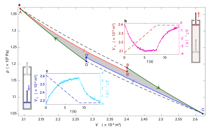
Figure 1: The finite-time Carnot cycle under the temperature combination ($T_{\mathrm{h}},T_{\mathrm{c}}$) $=(319.2.0,308.2)\mathrm{K}$. a. The Clapeyron pressure-volume ($p-V$) graph of the finite-time Carnot cycle. The red and blue lines show the finite-time isothermal expansion ($A\rightarrow B^{\prime}\rightarrow B$) with duration $\tau_{\mathrm{h}}$ and compression ($C\rightarrow C^{\prime}\rightarrow D$) with duration $\tau_{\mathrm{c}}$, and the green lines show the adiabatic processes ($B\rightarrow C$ and $D\rightarrow A$) without actual run. Two relaxation processes ($B^{\prime}\rightarrow B$ and $D^{\prime}\rightarrow D$) with the waiting time $2\tau_{\mathrm{relax}}$ are added to allow the system to reach the equilibrium with the thermal bath. The ideal Carnot cycle ($A\rightarrow B\rightarrow C\rightarrow D$) is presented as the gray dashed lines for reference. b-c. The gaseous volume $V_{\mathrm{h(c)}}(t)$ and the effective temperature trace $\Delta T_{\mathrm{h(c)}}(t)$ during the finite-time isothermal expansion and compression. The ideal gas is expanded or compressed with the constant speed $L(t)=L_{0}+\nu t$, with $\nu_{\mathrm{exp}}=20.00\mathrm{mm/s}$ and $\nu_{\mathrm{com}}=20.00\mathrm{mm/s}$ . The total time for the example cycle is $t_{\mathrm{tot}}=25.92\mathrm{s}$.

The Clapeyron pressure-volume ($p-V$) graph is shown in Fig. 1a with two finite-time isothermal processes (red and blue curves) and two no-run adiabatic processes (green curves). In each run, the system is immersed in the water bath for $10$ seconds to allow the initial equilibration of the gas system with the water bath. And the gas is expanded (red line $A\rightarrow B^{\prime}$ in Fig. 1b) or compressed (blue line $C\rightarrow D^{\prime}$ in Fig. 1c) in the two isothermal processes with constant speeds controlled by a step motor with the precision $\pm 0.02\mathrm{mm}$. The pressure traces $p(t)$ (red and blue curves) measured in the two processes deviates significantly from the equilibrium pressure (dashed black curve) due to the finite relaxation time $\tau_{\mathrm{relax}}=2.77\mathrm{s}$. After the expansion and compression, additional waiting time ($2\tau_{\mathrm{relax}}$) is added to allow the gas relaxing to the equilibrium state ($B^{\prime}\rightarrow B$ and $D^{\prime}\rightarrow D$). The four piston positions ($A,B,C,D$) are designed (see supplementary materials) for each temperature combination ($T_{\mathrm{h}}$,$T_{\mathrm{c}}$) to ensure the connection between the end ($B$ and $D$) of one finite-time isothermal process to the beginning ($C$ and $A$) of the other one with adiabatic processes. We run the engine cycles with 10 temperature combinations to span the Carnot efficiency from $\eta_{\mathrm{C}}=$0.0063 with the temperature combination $(313.2,311.2)\mathrm{K}$ to $\eta_{\mathrm{C}}=0.0343$ with $(319.2.0,308.2)\mathrm{K}$.

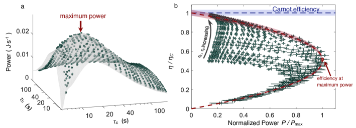
Figure 2: Power and efficiency of the finite-time Carnot engine under the temperature combination ($T_{\mathrm{h}},T_{\mathrm{c}}$) $=(319.2.0,308.2)\mathrm{K}$. a. Output power $P(\tau_{\mathrm{h}},\tau_{\mathrm{c}})$ as a function of operation time ($\tau_{\mathrm{h}},\tau_{\mathrm{c}}$). Each blue circle shows the output power averaged over 8 repeats of the measurement. The arrow shows the position of the maximum power with the control time $\tau_{\mathrm{h}}^{*}=13.32\mathrm{s}$ and $\tau_{\mathrm{c}}^{*}=12.60\mathrm{s}$. b. Efficiency-power tradeoff (blue circles with error bar). The dashed green curve shows the Carnot efficiency $\eta_{\mathrm{C}}=0.0343$, and the blue shadow presents the efficiency fluctuation due to temperature variation of the water bath during the experiments. The dashed red line shows the theoretical constraint [13] between the normalized efficiency $\widetilde{\eta}\equiv\eta/\eta_{\mathrm{C}}$ and power $\widetilde{P}\equiv P/P_{\mathrm{max}}$ with the upper bound $\widetilde{\eta}\leq 1-\left(1-\eta_{\mathrm{C}}\right)\widetilde{P}/[2\left(1+\sqrt{1-\widetilde{P}}\right)-\eta_{\mathrm{C}}\widetilde{P}]$ and the lower bound $\widetilde{\eta}\geq 1-\sqrt{1-\widetilde{P}}$ with the temperature fluctuation represented by the red shadow.

To evaluate the performance ( power and efficiency) of the designed cycle, we calculate the work performed in each process with the integral $W(t)=-\int p(t)\mathcal{A}dL(t)$. The heat exchange is obtained with the conservation of energy as $\Delta Q=-W+\Delta U$, where $\Delta U$ is the internal energy change of the gas. The important properties of the ideal gas is that its internal energy depends only on its temperature $T_{s}$, which is experimentally determined by the ideal gas law via the state equation $pV=nRT_{\mathrm{s}}$ with the amount of substance of gas in moles $n$ and the ideal gas constant $R$. The temperature deviations from the thermal bath $\Delta T_{\mathrm{h(c)}}(t)=T_{\mathrm{s}}(t)-T_{\mathrm{h(c)}}$ are illustrated with solid lines (cyan and purple) in Fig. 1b and 1c. The relaxation processes at the end of each isothermal process ensure the unchanged internal energy $\Delta U_{A\rightarrow B}=\Delta U_{C\rightarrow D}=0$, since the gas is nearly in equilibrium with the water bath $\Delta T_{\mathrm{h(c)}}(t)\approx 0$. The heat absorbed from the high(low)-temperature bath is measured directly via

$$Q_{\mathrm{h(c)}}=-W_{\mathrm{h(c)}}=\int_{0}^{\tau_{\mathrm{h(c)}}}p(t)\mathcal{A}\dot{L}(t)dt,$$ (1)

where $\tau_{\mathrm{h}}$ ($\tau_{\mathrm{c}}$) is the operation time for the isothermal expansion (compression) process $A\rightarrow B^{\prime}\rightarrow B$ ($C\rightarrow D^{\prime}\rightarrow D$). The total work extracted $W_{\mathrm{tot}}$ of the whole cycle is measured by the difference of heat exchanges, $W_{\mathrm{tot}}=Q_{\mathrm{h}}+Q_{\mathrm{c}}$. And the power is calculated as the total work extracted during a cycle divided by the total duration of the cycle, $P(\tau_{\mathrm{h}},\tau_{\mathrm{c}})=W_{\mathrm{tot}}$/($\tau_{\mathrm{h}}+\tau_{\mathrm{c}}$). The efficiency is given by the ratio between the extracted work $W_{\mathrm{tot}}$ and the input heat $Q_{\mathrm{h}}$ from the high-temperature thermal bath, $\eta(\tau_{\mathrm{h}},\tau_{\mathrm{c}})=W_{\mathrm{tot}}/Q_{\mathrm{h}}$. In Fig. 2a, we show how the power $P(\tau_{\mathrm{h}},\tau_{\mathrm{c}})$ changes with the two operation time $\tau_{\mathrm{h}}$ and $\tau_{\mathrm{c}}$ for one cycle under the temperature combination ($T_{\mathrm{h}},T_{\mathrm{c}}$) $=(319.2.0,308.2)\mathrm{K}$. The competition between the increase of work (equals to the gray area enclosed by the $p-V$ curve) and the increase of operation time results in the maximum power $P_{\mathrm{max}}=0.030\mathrm{J}\cdot\mathrm{s}^{-1}$ on the power surface with the control time $\tau_{\mathrm{h}}^{*}=13.32\mathrm{s}$ and $\tau_{\mathrm{c}}^{*}=12.60\mathrm{s}$ (red arrow in Fig. 2a).

Recently, much attentions are drawn to find the tradeoff between power and efficiency for finite-time thermodynamic cycles, e.g., Carnot cycle [7, 20]. Within the framework of the low-dissipation model [7, 9], a power and efficiency tradeoff relation [12, 11, 13] is predicted for finite-time Carnot cycle. Figure 2b shows the scatter plot of the normalized efficiency $\eta/\eta_{\mathrm{C}}$ and the normalized output power $P/P_{\mathrm{max}}$ for cycles with changing operation time $\tau_{\mathrm{h}}$ and $\tau_{\mathrm{c}}$. The error bars of each set $P$ and $\eta$ are obtained from 8 repeats of the experimental runs. The experimental data fall into the region enclosed by two margins of maximum and minimum efficiencies, which are illustrated as red dashed line with a red shadow area reflecting the fluctuation of the bath temperature in Fig. 2b. The data illustrates not only an upper bound for the achievable efficiency, but also a lower bound for the worst efficiency for the current finite-time Carnot cycle. The cycle achieves the Carnot efficiency $\eta_{\mathrm{C}}=0.0343$ with the increasing operation time $\tau_{\mathrm{c}}$ and $\tau_{\mathrm{h}}$ at the top left corner with a vanishing power.

The key quantity to evaluate the finite-time Carnot cycle is the efficiency at the maximum power $\eta_{\mathrm{EMP}}$, which was suggested as a physical efficiency limit independent of the properties of the working substance [5, 9]. We extract the efficiency at the maximum power $\eta_{\mathrm{EMP}}$ for all the temperature combinations in our experiment, and show its dependence on the Carnot efficiency in Fig. 3a. The obtained maximum efficiencies (markers with error bars) follow a simple relation $\eta_{\mathrm{EMP}}=(0.524\pm 0.034)\eta_{\mathrm{C}}+\mathcal{O}(\eta_{\mathrm{C}}^{2})$, which agrees well with the Curzon-Ahlborn efficiency[5] $\eta_{\mathrm{CA}}=1-\sqrt{1-\eta_{\mathrm{C}}}$ and the recent proposed bound [9, 8] $\eta_{\mathrm{C}}/(2-\eta_{\mathrm{C}})$ to the first order of the Carnot efficiency $\eta_{\mathrm{C}}$ as $\eta_{\mathrm{EMP}}=\eta_{\mathrm{C}}/2+\mathcal{O}(\eta_{\mathrm{C}}^{2})$. The coefficient $1/2$ was proved as a universal value independent of the system-specific features in the linear response regime due to the symmetry of the Onsager relations [7, 15]. Our experimental data provides the first demonstration of the leading order with the coefficient $1/2$.

The optimization of the cycle for maximum power is achieved by choosing the operation time $\tau_{h}$ and $\tau_{c}$. We determine the corresponding optimal operation time ($\tau_{\mathrm{h}}^{*},\tau_{\mathrm{c}}^{*}$) (markers in Fig. 3b) to reach the maximum power for cycles with all temperature combinations in the current experiment. The optimal time ($\tau_{\mathrm{h}}^{*},\tau_{\mathrm{c}}^{*}$) is verified to be in the regime where the $1/\tau$ scaling is valid [20, 22] (discussions in the supporting materials). With higher Carnot efficiency, less optimal operation time is needed to achieve the maximum efficiency and in turn more irreversibility is generated.

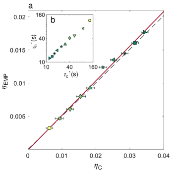
Figure 3: Optimized finite-time Carnot cycle with maximum power. a. Efficiency at maximum power (markers with error bars) as a function of Carnot efficiency. The red solid line shows the linear fit $\eta_{\mathrm{EMP}}=a+b\eta_{\mathrm{C}}$ yielding the parameters $a=\pm 7.0\times 10^{-4}$ and $b=0.524\pm 0.034$. The dashed black line shows the Curzon-Ahlborn efficiency $\eta_{\mathrm{CA}}=1-\sqrt{1-\eta_{\mathrm{C}}}$. b. Optimal operation time ($\tau_{\mathrm{h}}^{*},$$\tau_{\mathrm{c}}^{*}$) for the maximum power in the cycles with different Carnot efficiencies.

We have experimentally implemented the finite-time Carnot cycle with the dry air as working substance. For any given output power, we have shown the existence of the highest efficiency achieved with the designed operation time. Our results verify the existence of a universal relation of the efficiency at maximum power $\eta_{\mathrm{EMP}}=\eta_{\mathrm{C}}/2+\mathcal{O}(\eta_{\mathrm{C}}^{2})$ to the first order of the Carnot efficiency. We believe that our work will spur more experimental efforts into explore the finite-time thermodynamics.

This work is supported by the National Natural Science Foundation of China (NSFC) (Grants No. 12088101, No. 11534002, No. 11875049, No. U1930402, No. U1930403 and No. 12047549) and the National Basic Research Program of China (Grant No. 2016YFA0301201).

References

- [1] Carnot, S. Reflections on the Motive Power of Heat and on Machines Fitted to Develop that Power (J. Wiley, 1890).
- [2] Callen, H. B. Thermodynamics and an Introduction to Thermostatistics (John Wiley & Sons, 1985).
- [3] Andresen, B., Salamon, P. & Berry, R. S. Thermodynamics in finite time. Physics today 63 (1984).
- [4] Novikov, I. The efficiency of atomic power stations. J. Nucl. Energy 7, 125–128 (1958).
- [5] Curzon, F. L. & Ahlborn, B. Efficiency of a carnot engine at maximum power output. Am. J. Phys. 43, 22–24 (1975).
- [6] Andresen, B., Berry, R. S., Nitzan, A. & Salamon, P. Thermodynamics in finite time. i. the step-carnot cycle. Phys. Rev. A 15, 2086–2093 (1977).
- [7] Van den Broeck, C. Introduction to thermodynamics of irreversible processes. Phys. Rev. Lett. 95, 190602 (2005).
- [8] Schmiedl, T. & Seifert, U. Efficiency at maximum power: An analytically solvable model for stochastic heat engines. EPL (Europhysics Letters) 81, 20003 (2007).
- [9] Esposito, M., Kawai, R., Lindenberg, K. & Van den Broeck, C. Efficiency at maximum power of low-dissipation carnot engines. Phys. Rev. Lett. 105, 150603 (2010).
- [10] Tu, Z. C. Efficiency at maximum power of feynman's ratchet as a heat engine. J. Phys. A: Math. Theor. 41, 312003 (2008).
- [11] Ryabov, A. & Holubec, V. Maximum efficiency of steady-state heat engines at arbitrary power. Phys. Rev. E 93, 050101 (2016).
- [12] Shiraishi, N., Saito, K. & Tasaki, H. Universal trade-off relation between power and efficiency for heat engines. Phys. Rev. Lett. 117, 190601 (2016).
- [13] Ma, Y.-H., Xu, D., Dong, H. & Sun, C.-P. Universal constraint for efficiency and power of a low-dissipation heat engine. Phys. Rev. E 98, 042112 (2018).
- [14] Prigogine, I. Introduction to the Thermodynamics of Irreversible Processes (Wiley, 1968), 3rd edition edn.
- [15] Seifert, U. Stochastic thermodynamics, fluctuation theorems and molecular machines. Rep. Prog. Phys 75, 126001 (2012).
- [16] Chen, L. & Yan, Z. The effect of heat-transfer law on performance of a two-heat-source endoreversible cycle. J. Chem. Phys. 90, 3740–3743 (1989).
- [17] Chen, Y. H., Chen, J.-F., Fei, Z. & Quan, H. T. A microscopic theory of curzon-ahlborn heat engine. arXiv (2021).
- [18] Holubec, V. & Ryabov, A. Maximum efficiency of low-dissipation heat engines at arbitrary power. J. Stat. Mech.: Theory E. 2016, 073204 (2016).
- [19] Blickle, V. & Bechinger, C. Realization of a micrometre-sized stochastic heat engine. Nat. Phys. 8, 143–146 (2011).
- [20] Martínez, I. A. et al. Brownian carnot engine. Nat. Phys. 12, 67–70 (2015).
- [21] Rossnagel, J. et al. A single-atom heat engine. Science 352, 325–329 (2016).
- [22] Ma, Y.-H., Zhai, R.-X., Chen, J., Sun, C. P. & Dong, H. Experimental test of the 1/t-scaling entropy generation in finite-time thermodynamics. Phys. Rev. Lett. 125, 210601 (2020).