Propagation with Adaptive Mask then Training for Node Classification on Attributed Networks

Abstract

Node classification on attributed networks is a semi-supervised task that is crucial for network analysis. By decoupling two critical operations in Graph Convolutional Networks (GCNs), namely feature transformation and neighborhood aggregation, some recent works of decoupled GCNs could support the information to propagate deeper and achieve advanced performance. However, they follow the traditional structure-aware propagation strategy of GCNs, making it hard to capture the attribute correlation of nodes and sensitive to the structure noise described by edges whose two endpoints belong to different categories. To address these issues, we propose a new method called the Propagation with Adaptive Mask then Training (PAMT). The key idea is to integrate the attribute similarity mask into the structure-aware propagation process. In this way, PAMT could preserve the attribute correlation of adjacent nodes during the propagation and effectively reduce the influence of structure noise. Moreover, we develop an iterative refinement mechanism to update the similarity mask during the training process for improving the training performance. Extensive experiments on four real-world datasets demonstrate the superior performance and robustness of PAMT.

We propose a new semi-supervised method for the node classification on attributed networks.

We propagate the label information on the weighted graph by combining attribute feature and topology feature.

We develop an iterative refinement to boost training and use a momentum-based strategy for a stable training.

Extensive experiments demonstrate the superiority on performance and the robustness to structure noise.

1 Introduction

Attributed networks have been widely used to model various entities and their relationships in the real world, such as users and their social connections in social networks. Due to the complex topology structure and abundant attribute features, graph mining tasks on attributed networks are much more challenging. In this work, we address a fundamental and essential task, the semi-supervised node classification (SSNC) on attributed networks, which has a wide range of applications such as social influence analysis in social networks [1, 2].

Numerous techniques have been proposed for SSNC, e.g., network embedding-based methods [3] and label propagation-based methods [4], etc. Among which, Graph Convolutional Network (GCN) based methods [5, 6, 7, 8] have gained great success with high performance. The core component of GCN-based models is the graph convolution layer. Each graph convolution layer includes two important operations, namely neighbor aggregation and feature transformation. Neighbor aggregation is used for aggregating features from the neighborhood to update node representations, while the function of feature transformation is to extract new representations from the previous features [9]. These operations are actually coupled in a graph convolution layer for aggregating and transferring the information of neighborhood nodes to learn the node representations.

Despite effectiveness, recent studies indicate that the coupled design of GCN could lead to some problems in practice, such as over-smoothing [10, 11] and inefficient training [12, 13]. A natural solution to the above issues is to decouple the operations of neighbor aggregation and feature transformation. Following this strategy, several effective models [12, 13] have been proposed, termed decoupled GCNs [9]. The rationale of decoupled GCNs is to remove the nonlinear activation functions and collapse the matrices (adjacency matrix and parameter matrices) from the graph convolution layers. In this way, the neighbor aggregation and feature transformation can be considered as two separate modules. Such decoupled design could permit deeper propagation without leading to over-smoothing and exhibits superior performance for SSNC on attributed networks [12].

Although decoupled GCNs simplify the design of GCN-based models and achieve significant improvements in terms of accuracy and efficiency, we observe that they still follow the traditional structure-aware propagation mechanism of GCN-based methods, i.e., only utilizing the adjacency matrix to aggregate information. Thus, they suffer from the following limitations on attributed networks:

1. It is hard to capture the correlation of attribute features. The attributed information is one of the essential features in attributed networks. Nodes with similar attributes tend to belong to the same category. However, existing propagation mechanisms of decoupled GCNs are only topology structure-aware and ignore the attribute features of nodes. Hence, the model is hard to capture the correlation of attribute features between nodes on attributed networks. In addition, recent studies have shown that the topology structure-aware propagation mechanism could destroy the attribute information of nodes [14, 15]. Thus, the topology structure-aware propagation mechanism would limit the model performance for node classification on attributed networks.

2. They are sensitive to the graph structure noise. The graph structure noise is described by edges connecting nodes of different categories [9]. During the propagation process, this topology structure-aware propagation mechanism assigns large weights to the adjacent nodes no matter whether they belong to the same category, which will hurt the performance, causing the model to be sensitive to the graph structure noise, as demonstrated in recent works [9].

To address the above issues, in this work, we propose a novel method called Propagation with Adaptive Mask then Training (PAMT). PAMT is inspired by [9] which improves the training efficiency of decoupled GCNs by introducing a two-step training framework. The key idea is to integrate the attribute similarity of adjacent nodes into the structure-aware propagation process, so that the attribute correlation of the adjacent nodes could be well captured and the influence of structure noise could be effectively reduced.

There are three main stages in the proposed PAMT: 1) It generates a similarity mask based on attribute features and labeled data to represent the similarity of each node pair. 2) A propagation matrix is generated based on the similarity mask and adjacency matrix, and the matrix is further used in the label propagation procedure to create soft labels for training the classifier. 3) PAMT enhances the training process by using an iterative refinement mechanism to alternately update the similarity mask and the soft labels. In addition, a momentum-based update strategy [16] is applied in the process of generating new soft labels so as to gain a stable training.

Our main contributions are summarized as follows:

• We propose a new method called PAMT for node classification on attributed networks, whose key idea is to utilize the attribute information to strengthen the existing propagation operation of decoupled GCNs.

• We develop an iterative refinement mechanism applied in the training process to improve the training performance, and utilize a momentum-based update strategy to gain a stable training.

• Extensive experiments on four real-world datasets demonstrate the superiority on performance and robustness to structure noise of PAMT over the baselines.

2 Related Work

In this section, we review related works on GCNs and decoupled GCNs, and highlight the difference of our method.

2.1 GCN-based Approaches

Many follow-up methods have been proposed recently to improve the efficiency of the vanilla GCN [6]. GraphSAGE [5] develops a sampling-based aggregation operation to overcome the memory overflow issue of GCN when the graph is in large scale. GAT [7] introduces an attention mechanism into the aggregation operation to capture the feature similarity between adjacent nodes, that are overlooked in the vanilla GCN. For improving the flexibility of aggregation operation of GCN, Xu et al. [8] propose JK-Nets to selectively exploit information from neighborhoods of different locality. GCN suffers from the over-smoothing problem [10] when the graph convolutional layers get deeper, and a possible solution is to balance the information obtained between the layers [17]. Li et al. [18] propose DeeperGCN by using a generalized aggregation function to improve the training performance.

Integrating attribute information. Besides GAT [7] that utilizes attribute information to guide the neighborhood aggregation, there are several GCN-based studies that combine attribute information and topology information for achieving high performance. One common way is to generate a $k$-nearest neighbor ($k$NN) graph based on the attribute similarity matrix of nodes. To obtain a similarity matrix, various methods have been adopted to calculate the similarity of nodes according to their attribute features, such as Cosine Similarity [19, 14, 20] and Heat Kernel [19]. In addition to the $k$NN graph, recent studies utilize the attribute information to estimate the label similarity matrix [21] or the block matrix [22] and further combine them with the adjacency matrix for enhancing the effort of aggregation operation. For more details on GCN-based approaches, we refer the readers to a survey [23].

Different from the above GCN-based methods, the proposed PAMT adopts the decoupled design that uses independent modules for information propagation and feature transformation. PAMT also develops an iterative refinement mechanism to dynamically adjust the attribute similarity mask during the training process which makes a great difference from the above methods.

2.2 Decoupled GCN-based Approaches

The two important operations of GCN, neighbor aggregation and feature transformation, are coupled in the graph convolution layer in the original design. Recent studies [12, 11, 24, 13] have demonstrated that such coupled design may limit the model’s capability of deeply capturing the topology feature and cause over-smoothing issue.

To tackle the above issues, Wu et al. [13] propose SGCN by removing the nonlinear activation functions and collapsing weight matrices between consecutive graph convolutional layers. APPNP [12] combines the personalized PageRank and the neural network classifier to simplify GCN by treating the neighbor aggregation and feature transformation as independent modules. Dong et al. [9] summarize studies based on the idea of decoupling neighbor aggregation and feature transformation, and call these methods the decoupled GCNs. The authors theoretically analyze the relationship between decoupled GCNs and label propagation (LP) [25], and propose a Propagation then Training (PT) method and an improved version, Propagation then Training Adaptively (PTA). PT generates the soft labels for unlabeled nodes and trains the neural network classifier using the obtained labels in a supervised learning manner. PTA extends PT by introducing an adaptive weighting strategy into the training stage to further improve the model performance.

We observe that these methods ignore the attribute information during the propagation, causing them sensitive to the structure noise. To this end, our PAMT utilizes not only topology features but also attribute features when propagating information on networks, and improves the model robustness.

3 Preliminaries

In this section, we first formulate the task of semi-supervised node classification on attributed networks, then we briefly review the vanilla GCN and decoupled GCNs. Finally, we introduce the PT method [9] in detail, which is highly related to our work.

3.1 Problem Formulation

Consider an unweighted and undirected attributed graph $G=(V,E,\mathbf{X})$, where $V$ and $E$ are the sets of nodes and edges, respectively. $n=|V|$ denotes the number of nodes. $\mathbf{X}\in\mathbb{R}^{n\times d}$ is the feature matrix of node attributes, where $d$ is the dimension of each feature vector. Let $\mathbf{A}$ be the adjacency matrix, i.e., $\mathbf{A}_{ij}=1$ if there exists an edge between nodes $v_{i}$ and $v_{j}$, otherwise, $\mathbf{A}_{ij}=0$. Given a small set of labeled nodes denoted by $V_{L}$, the task of semi-supervised node classification is to predict the labels for all $v\in V\backslash V_{L}$ .

3.2 Vanilla GCN and Decoupled GCNs

The rationale of the vanilla GCN is to simultaneously capture the topological information of the graph and the attribute features of nodes by stacking several graph convolution layers. The graph convolution layer can be written as [6]:

$$\mathbf{H}^{(l+1)}=\boldsymbol{\sigma}(\hat{\mathbf{A}}\mathbf{H}^{(l)}\mathbf{W}^{(l)}),$$ (1)

where $\hat{\mathbf{A}}=\widetilde{\mathbf{D}}^{-\frac{1}{2}}\widetilde{\mathbf{A}}\widetilde{\mathbf{D}}^{-\frac{1}{2}}$ is the normalized adjacency matrix, $\widetilde{\mathbf{A}}$ is the adjacency matrix with a self loop on each node, and $\widetilde{\mathbf{D}}$ denotes the corresponding diagonal degree matrix, i.e., $\widetilde{\mathbf{D}}_{ii}=\sum_{j}\widetilde{\mathbf{A}}_{ij}$. $\mathbf{H}^{(l)}$ is the feature matrix of the $l^{th}$ GCN layer, and $\mathbf{H}^{(0)}=\mathbf{X}\cdot\mathbf{W}^{(l)}$ represents the learnable weight matrix of the $l^{th}$ GCN layer, and $\boldsymbol{\sigma}$ denotes the activation function.

According to Equation 1, there are two coupled operations in each graph convolution layer, namely neighbor aggregation and feature transformation. However, such coupled design limits the capability of deeply capturing the topology information and easily leads to over-smoothing problem. A rational solution is to decouple the two operations, termed the decoupled GCNs [9]:

$$\hat{\mathbf{Y}}=softmax(\bar{\mathbf{A}}\boldsymbol{f}_{\theta}(\mathbf{X})),$$ (2)

where $\boldsymbol{f}_{\theta}$ indicates the neural network classifier (e.g., MLP [26]), and $\bar{\mathbf{A}}=\sum\varphi_{k}\hat{\mathbf{A}}^{k}$ denotes the operation of propagating $k$ times through $\hat{\mathbf{A}}$ by a propagation strategy (e.g., personalized PageRank in APPNP). Each entry $\bar{\mathbf{A}}_{ij}$ denotes the proximity of nodes $i$ and $j$ in the graph. It has been demonstrated that such decoupled design can improve the performance of node classification [9, 12].

3.3 The PT Method

As shown in Equation 2, the decoupled GCNs can be regarded as a combination of propagation module and classifier module. Based on such design, Dong et al. [9] propose a novel method called Propagation then Training (PT). PT contains two main stages, i.e., the training stage and the inference stage. In the training stage, PT generates soft labels by label propagation, and trains the neural network classifier $\boldsymbol{f}_{\theta}$ based on the soft labels. The objective function is as follows:

$$\boldsymbol{L}_{PT}(\theta) =\boldsymbol{\ell}(\boldsymbol{f}_{\theta}(\mathbf{X}),\mathbf{Y}_{soft}),$$ (3)

where $\mathbf{Y}_{soft}=\bar{\mathbf{A}}\mathbf{Y}_{L}$ indicates the soft labels generated by $\bar{\mathbf{A}}$ and the observed labels $\mathbf{Y}_{L}$, and $\boldsymbol{\ell}(\cdot)$ denotes the cross entropy loss. In the inference stage, PT generates the final prediction for nodes as follows:

$$\hat{\mathbf{Y}}=\bar{\mathbf{A}}\cdot softmax(\boldsymbol{f}_{\theta}(\mathbf{X})).$$ (4)

It indicates that for each node, PT first generates the soft labels according to the final output of the neural network classifier after softmax. Then, PT aggregates the soft labels of its $k$-hop neighbors (if propagate $k$ times) based on $\bar{\mathbf{A}}$. Finally, PT outputs the final prediction labels for each node by aggregating information of the neighbors.

4 The Proposed PAMT

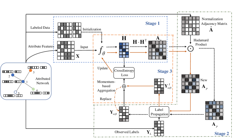
Figure 1: The framework of PAMT. It consists of three stages. In Stage 1, PAMT generates the similarity mask of nodes based on the attribute features and the labeled data. In Stage 2, PAMT integrates the similarity mask into the adjacency matrix by Hadamard product to create the propagation matrix, then generates the soft labels based on the observed labels and propagation adjacency matrix using label propagation. In Stage 3, PAMT develops an iterative refinement mechanism to alternately update the similarity mask and soft labels for improving the training performance.

The goal of our Propagation with Adaptive Mask then Training (PAMT) is to train a superior neural network classifier $\boldsymbol{f}_{\theta}$ for node classification using the attribute features of nodes and the topology features of the graph. The framework of PAMT is shown in Figure 1. Specifically, PAMT contains three stages: calculate the attribute similarity mask, propagate labels, and train with an iterative refinement mechanism.

4.1 Generating the Similarity Mask

For the node classification task on attribute networks, the node attribute features are critical information. In general, nodes belonging to the same class tend to have similar attribute features. Thus, our PAMT utilizes the attribute information to generate an attribute similarity mask to capture the similarity between nodes. On the other hand, the attribute similarity mask can also refine the topological information based on attribute features to reduce the impact of structure noise during the propagation.

To guarantee a good quality of the similarity mask and keep simplicity on the model, we use a neural network classifier $\boldsymbol{f}_{\theta}$ (MLP in this paper) initialized with the labeled data to calculate the attribute similarity mask. For a randomly initialized $\boldsymbol{f}_{\theta}$, we first train on the labeled data with fixed training epochs. Then we get the representation matrix $\mathbf{H}$ of nodes through $\boldsymbol{f}_{\theta}$:

$$\mathbf{H}=\boldsymbol{f}_{\theta}(\mathbf{X}).$$ (5)

And the attribute similarity mask $\mathbf{A}_{s}$ is calculated as follows:

$$\mathbf{A}_{s}=\mathbf{H}\mathbf{H}^{\top}.$$ (6)

There are two motivations for this design: 1) after training with labeled data, $\boldsymbol{f}_{\theta}$ has a good classification performance, as shown in [9], so the output of $\boldsymbol{f}_{\theta}$ has the ability to ensure the quality of $\mathbf{A}_{s}$; 2) the goal of PAMT is to train a superior $\boldsymbol{f}_{\theta}$, thus initializing $\boldsymbol{f}_{\theta}$ with the labeled data to calculate $\mathbf{A}_{s}$ does not increase the model complexity as there is no additional parameter to be added to the model.

4.2 Propagation with Similarity Mask

The goal of stage 2 is to build a propagation matrix $\mathbf{A}_{p}$ that simultaneously preserves the attribute information and topology information of nodes, and propagate the observed labels on $\mathbf{A}_{p}$ using label propagation to create the soft labels for unlabeled nodes.

For calculating $\mathbf{A}_{p}$, we combine $\mathbf{\hat{A}}$ and $\mathbf{A}_{s}$ using Hadamard product:

$$\mathbf{A}_{p}=\hat{\mathbf{A}}\odot\mathbf{A}_{s}.$$ (7)

The meanings of the above operation are twofold. On the one hand, the elements of $\mathbf{\hat{A}}$ and $\mathbf{A}_{s}$ represent the topology similarity and attribute similarity of the node pairs, respectively. Thus the elements of $\mathbf{A}_{p}$ preserve these two types of similarity for node pairs, which enhances the representation ability of the adjacency matrix. On the other hand, $\mathbf{\hat{A}}$ only contains the first-order neighbors of nodes, so that using Hadamard product to combine $\mathbf{\hat{A}}$ and $\mathbf{A}_{s}$ could preserve the sparsity of $\mathbf{\hat{A}}$, which will reduce the time complexity of the propagation operation.

After the above process, we gain a weighted matrix $\mathbf{A}_{p}$. We further run a propagation operation with observed labels $\mathbf{Y}_{L}$ to generate the soft labels $\mathbf{Y}_{soft}$:

$$\mathbf{Y}_{soft}=\bar{\mathbf{A}}_{p}\mathbf{Y}_{L}.$$ (8)

The propagation method we adopt is the approximate personalized PageRank for its high computational efficiency and superior performance [9, 12]. $\bar{\mathbf{A}}_{p}$ represents the matrix of $\mathbf{A}_{p}$ after propagation, calculated as follows [9]:

$$\bar{\mathbf{A}}_{p}=(1-\alpha)^{K}\mathbf{A}_{p}^{K}+\alpha\sum_{k=0}^{K-1}(1-\alpha)^{k}\mathbf{A}_{p}^{k},$$ (9)

where $\alpha$ is the propagation bias and $K$ denotes the number of propagations.

4.3 Iterative Refinement Mechanism

The goal of stage 3 is to train a superior $\boldsymbol{f}_{\theta}$ with $\mathbf{Y}_{soft}$. The objective function of PAMT is described as follows:

$$\boldsymbol{L}_{PAMT}(\theta)=\boldsymbol{\ell}(\boldsymbol{f}_{\theta}(\mathbf{X}),\mathbf{Y}_{soft}),$$ (10)

where $\boldsymbol{\ell}(\cdot)$ indicates the cross entropy loss.

However, $\mathbf{Y}_{soft}$ is generated by using label propagation only once during the whole training phase, and $\boldsymbol{f}_{\theta}$ can not be well trained because $\mathbf{Y}_{soft}$ could not precisely represent the soft labels of nodes. To tackle the above issue, inspired by some researches that do refinement iteratively in a mutual way [27, 28, 29], we develop an iterative refinement mechanism to improve the training performance of model $\boldsymbol{f}_{\theta}$. In this mechanism, $\boldsymbol{f}_{\theta}$ will be updated periodically when meeting the update condition that epoch $t$ meets $t\%t_{u}=0$ ( $t_{u}$ is a fixed number). Then, the new $\mathbf{A}_{s}$ can be calculated based on the updated $\boldsymbol{f}_{\theta}$ according to Equation 5 and Equation 6. Finally, PAMT calculates $\mathbf{Y}^{t}_{soft}$ at epoch $t$ according to Equation 7 and Equation 8. Differing from previous works [28, 29] that update $\mathbf{Y}{{}_{soft}}$ by setting $\mathbf{Y}{{}_{soft}}\leftarrow\mathbf{Y}^{t}_{soft}$, we perform a momentum-based strategy [16] to update $\mathbf{Y}{{}_{soft}}$ to avoid instability and information loss:

$$\mathbf{Y}{{}_{soft}}\leftarrow\beta\mathbf{Y}{{}_{soft}}+(1-\beta)\mathbf{Y}^{t}_{soft},$$ (11)

where $\beta\in[0,1)$ is the momentum coefficient to control the contribution to the label update. The overall learning algorithm of PAMT is summarized in Algorithm 1.

The intuition is that the well-trained $\boldsymbol{f}_{\theta}$ will enhance the quality of $\mathbf{Y}{{}_{soft}}$, and high quality $\mathbf{Y}{{}_{soft}}$ will improve the training performance of $\boldsymbol{f}_{\theta}$. As the training process goes on, both $\boldsymbol{f}_{\theta}$ and $\mathbf{Y}{{}_{soft}}$ will be promoted. Since the updates of $\boldsymbol{f}_{\theta}$ and $\mathbf{Y}{{}_{soft}}$ are iterative, we call it an iterative refinement mechanism. In addition, the similarity mask $\mathbf{A}_{s}$ generated by $\boldsymbol{f}_{\theta}$ is changing during the training process. Hence, $\mathbf{A}_{s}$ could be regarded as an adaptive similarity mask.

Algorithm 1 The learning algorithm of PAMT

1:Adjacency matrix $\mathbf{A}$; Feature matrix $\mathbf{X}$; Observed labels $\mathbf{Y}_{L}$;

2:Neural network classifier $\boldsymbol{f}_{\theta}$ ;

3:Initialize $\boldsymbol{f}_{\theta}$ with labeled data;

4:Generate the attribute similarity mask $\mathbf{A}_{s}$ by Equation 6;

5:Generate soft label ${\mathbf{Y}}_{soft}$ by Equation 8;

6:for $t=1$ to $Epoch_{max}$ do

7:     if $t\%t_{u}=0$ then

8:         Update $\mathbf{A}_{s}$ by Equation 6

9:         Generate $\mathbf{Y}^{t}_{soft}$ by Equation 8

10:         Update ${\mathbf{Y}}_{soft}$ by Equation 11

11:     end if

12:     Calculate loss $\boldsymbol{L}_{PAMT}(\theta)$ by Equation 10

13:     Optimize $\theta$ by minimizing $\boldsymbol{L}_{PAMT}$ with gradient descent

14:end for

15:return Neural network classifier $\boldsymbol{f}_{\theta}$;

After the training process, we generate the final prediction using $\boldsymbol{f}_{\theta}$ based on Equation 4 for predicting the labels of unlabeled nodes.

4.4 Complexity Analysis

The time complexity of PAMT could be analyzed through the two phases: the training phase and inference phase.

Suppose $\boldsymbol{f}_{\theta}$ is an MLP with one hidden layer of dimension $f$. In the training phase, if the training epoch $t$ does not meet the update condition, the time complexity of each epoch will be $\Phi(\boldsymbol{f}_{\theta}(\mathbf{X}))=O(nf(d+c))$, where $\Phi(\boldsymbol{f}_{\theta}(\mathbf{X}))$ represents the complexity of operation $\boldsymbol{f}_{\theta}(\mathbf{X})$, $n$ represents the number of nodes, $c$ represents the number of labels and $d$ represents the dimension of raw attribute features; if $t$ meets the condition, the complexity of each epoch will be consist of four parts: $\Phi(\mathbf{H}\mathbf{H}^{\top})+\Phi(\hat{\mathbf{A}}\odot\mathbf{A}_{s})+\Phi(\mathbf{A}_{p}\mathbf{Y}_{V_{L}})+\Phi(\boldsymbol{f}_{\theta}(\mathbf{X}))=O(n^{2}(2c+1)+nf(d+c))$.

In the inference phase, the complexity is $\Phi(\boldsymbol{f}_{\theta}(\mathbf{X}))+\Phi(\bar{\mathbf{A}}\mathbf{H})=O(n^{2}c+nf(d+c))$. Sparse matrix techniques could be used for optimizing the above operations except $\boldsymbol{f}_{\theta}(\mathbf{X})$ and $\mathbf{H}\mathbf{H}^{\top}$. Since $\mathbf{H}$ is a dense matrix, the complexity of $\mathbf{H}\mathbf{H}^{\top}$ will be high when the number of nodes is large. And the similarity mask is created by $\mathbf{H}\mathbf{H}^{\top}$, thus an important future work is to optimize the method of generating the similarity mask.

5 Experiments

In this section, we first introduce the experimental setup, including benchmark datasets, baseline methods and implementation details. Then we conduct extensive experiments to answer the following questions: 1) How does PAMT perform as compared with existing baselines in the semi-supervised node classification task? 2) How does the robustness of PAMT to the graph structure noise, comparing with existing baselines? 3) How do the key designs of PAMT help improve the model performance? 4) How do the key hyper-parameters affect the performance of PAMT?

5.1 Experimental Setup

Datasets. Following [9], we choose four widely used attribute network datasets for experiments, including Cora_ML [30], Citeseer [31], Pubmed [32] and Microsoft Academic [33]. Cora_ML, Citeseer, Pubmed are citation networks and Microsoft Academic (MS_ACA) is a co-authorship network. Nodes in these networks represent entities (e.g., papers in citation networks) and edges represent relationships between entities (e.g., citation relationships in citation networks). The statistics of datasets are reported in Table 1. For the semi-supervised node classification setting, following [9], we split each dataset into three partitions: training set, early-stopping set and test set. Each class has 20 labeled nodes in the training set. All the datasets are available at the website from [9].

Baselines. We choose the baselines from the following three categories: GCN-based methods, decoupled GCN-based methods and PT-based methods. For GCN-based methods, we select GCN [6], GAT [7] and RGCN [34]. For decoupled GCN-based methods, we select SGCN [13] and APPNP [12]. For PT-based methods, we select PTS [9] and PTA [9]. For variants of PAMT, we use PAMT_r to represent a variant of PAMT that uses a randomly initialized $\boldsymbol{f}_{\theta}$ to generate the similarity mask.

Implementation Details. The experiments were conducted on a server with 1 I9-9900k CPU, 1 RTX 2080TI GPU and 64G RAM. The codes of all methods are based on Python 3.8 and Pytorch 1.8.0. We use the Adam optimizer [35] for learning the parameters of all models. The hyper-parameters of the baselines use the recommendation settings in their official implementation. For PAMT, we determine the hyper-parameters by grid search. The detailed hyper-parameter settings of PAMT on each dataset are summarized in Table 2. Here $dim$ denotes the dimension of hidden layer of $\boldsymbol{f}_{\theta}$; $wd$ and $lr$ denote the weight-decay coefficient and learning rate, respectively; $drop$ denotes the dropout rate.

Table 1: Statistics on datasets.

Dataset	#Nodes	#Edges	#Features	#Classes
Cora_ML	2,810	7,981	2,879	7
Citeseer	2,110	3,668	3,703	6
Pubmed	19,717	44,324	500	3
MS_ACA	18,333	81,894	6,805	15

Table 2: Hyper-parameters of PAMT on each dataset.

Dataset	$dim$	$\alpha$	$wd$	$lr$	$\beta$	$K$	$drop$	$t_{u}$
Cora_ML	128	0.10	0.025	0.05	0.50	10	0.20	30
Citeseer	128	0.15	0.055	0.10	0.25	10	0.15	20
Pubmed	128	0.10	0.015	0.10	0.10	10	0.35	10
MS_ACA	256	0.10	0.010	0.05	0.10	10	0.35	10

Table 3: Results of all models in terms of accuracy (%) on different datasets. The best results are in bold and the second bests are underlined.

Method	Cora_ML	Citeseer	Pubmed	MS_ACA
GCN	82.90 $\pm$ 0.41	73.56 $\pm$ 0.59	76.75 $\pm$ 0.63	91.26 $\pm$ 0.18
GAT	83.46 $\pm$ 0.58	72.79 $\pm$ 0.24	78.97 $\pm$ 0.24	91.43 $\pm$ 0.05
RGCN	84.18 $\pm$ 0.15	72.83 $\pm$ 0.15	78.77 $\pm$ 0.11	92.61 $\pm$ 0.08
SGCN	77.44 $\pm$ 0.87	75.89 $\pm$ 0.36	70.68 $\pm$ 1.50	90.83 $\pm$ 0.17
APPNP	85.63 $\pm$ 0.18	75.51 $\pm$ 0.35	78.86 $\pm$ 0.57	92.41 $\pm$ 0.19
PTS	85.62 $\pm$ 0.37	75.74 $\pm$ 0.35	78.79 $\pm$ 0.69	91.85 $\pm$ 0.17
PTA	85.50 $\pm$ 0.22	75.72 $\pm$ 0.41	79.08 $\pm$ 0.77	92.72 $\pm$ 0.09
PAMTr	83.27 $\pm$ 0.84	69.01 $\pm$ 0.63	76.67 $\pm$ 0.56	92.35 $\pm$ 0.48
PAMT	86.01 $\pm$ 0.32	76.98 $\pm$ 0.24	79.38 $\pm$ 0.44	92.92 $\pm$ 0.14

5.2 Performance Comparison

We first compare the performance of PAMT with the baselines for the semi-supervised node classification task. Table 3 reports the main results of all models in terms of accuracy and standard deviation with random data splits. In general, PAMT outperforms all the baselines on every datasets. Specifically, PAMT beats PT-based methods, which indicates that introducing the attribute features into the propagation during the training phase can improve the training performance. In addition, PAMT outperforms its variant PAMT_r, which indicates initializing $\boldsymbol{f}_{\theta}$ with the labeled data is helpful to increase the model performance.

We also observe that, in general, the decoupled GCN-based methods (e.g. APPNP and PTA) outperform GCN-based methods (e.g. GCN and GAT) over all datasets. This is mainly because decoupled GCN-based methods can allow the information propagate deeper on networks than GCN-based methods and exhibits the superiority of the decoupled design.

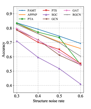
(a) Cora_ML

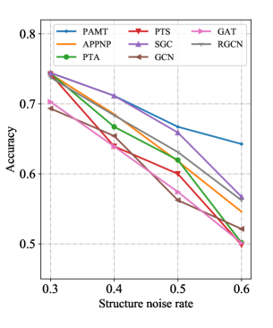
(b) Citeseer

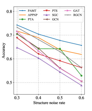
(c) Pubmed

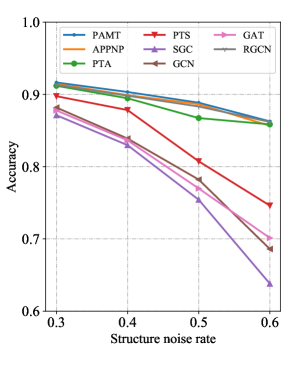
(d) MS_ACA

Figure 2: Performance comparison after adding different rates of structure noise.

5.3 Comparison on Robustness to Structure Noise

We conduct experiments to further study the model robustness to structure noise. As mentioned before, we regard the edge connecting nodes of different labels as structure noise. So that for adding structure noise to the graph, we randomly remove the edge connecting nodes of the same label and add the edge connecting nodes of the different labels which is following the work of Dong et al. [9]. Our goal is to explore the performance of all models under different rates of structure noise. Since the original rates of structure noise over all datasets are less than 0.3, our experiments begin the structure noise rate at 0.3 and end at 0.6. Figure 2 reports the results, from which we have the following observations:

1) PAMT exhibits higher robustness to the structure noise, outperforming other methods on all the four datasets. These results validate that the design of introducing the attribute information into the propagation operation is beneficial to improve the model robustness. On MS_ACA, the performance of PAMT, PTA, APPNP and RGCN are very close. This is mainly because MS_ACA provides abundant attribute features (refer to Table 1) which are enough to train a competitive classifier for prediction.

2) Decoupled GCN-based methods exhibit higher robustness to structure noise than GCN-based methods. This may due to that decoupled GCN-based methods can utilize more information based on the propagation process. In addition, APPNP and PTA outperform SGC on Cora_ML, Pubmed and MS_ACA. This is mainly because the propagation method of APPNP and PTA is the personalized PageRank which will retain their own features of the nodes. In this way, the influence of structure noise will be reduced.

3) GCN-based methods, like GCN and GAT, are sensitive to structure noise. This is because they obey the coupled design that limits the ability of deeply capturing the information of networks, and they only utilize information from the first-order neighbors, making them easily be disturbed by structure noise.

Table 4: PAMT and its variants.

Method	Similarity mask-based propagation	Iterative refinement mechanism	Momentum-based update strategy
PTS	$\times$	$\times$	$\times$
PAMT0	✓	$\times$	$\times$
PAMT1	✓	✓	$\times$
PAMT	✓	✓	✓

Table 5: Ablation study on PAMT.

Method	Cora_ML	Citeseer	Pubmed	MS_ACA
PTS	85.62 $\pm$ 0.37	75.74 $\pm$ 0.35	78.79 $\pm$ 0.69	91.85 $\pm$ 0.17
PAMT0	85.52 $\pm$ 0.34	76.62 $\pm$ 0.32	78.97 $\pm$ 0.34	92.43 $\pm$ 0.38
PAMT1	85.66 $\pm$ 0.36	76.82 $\pm$ 0.12	79.12 $\pm$ 0.29	92.60 $\pm$ 0.36
PAMT	86.01 $\pm$ 0.32	76.98 $\pm$ 0.24	79.38 $\pm$ 0.44	92.92 $\pm$ 0.14

5.4 Ablation Study

In this subsection, we conduct experiments to validate the contributions of the key designs of PAMT to the model performance. As mentioned in Section 4, there are three key designs in PAMT: similarity mask-based propagation, iterative refinement mechanism and momentum-based update strategy. If we remove all these components, PAMT will degenerate to PTS. For validating the effectiveness of the above designs, we propose two variants of PAMT: PAMT₀ and PAMT₁. In PAMT₀, only the similarity mask-based propagation is preserved, while PAMT₁ only removes the momentum-based update strategy of PAMT. Characteristics of PAMT and its variants are summarized in Table 4.

The results are reported in Table 5, from which we have the following observations: 1) In general, PAMT₀ and PAMT₁ outperform PTS, showing that both the similarity mask-based propagation and the iterative refinement mechanism can help to train a high-quality neural network classifier. 2) PAMT₁ beats PAMT₀ on all datasets, exhibiting the importance of the iterative refinement mechanism. 3) PAMT outperforms PAMT₁. The reason may be that the direct replacement strategy is used in PAMT₁, which may lead instability and cause information loss. This phenomenon also indicates that the momentum-based update strategy can improve the model performance.

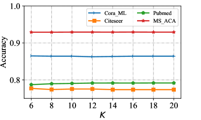
(a) On propagation step $K$

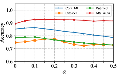
(b) On propagation bias $\alpha$

Figure 3: Performance under different parameters.

5.5 Parameter Study

We continue to conduct experiments to examine the sensitivity of the key parameters on the model performance, the propagation step $K$ and the propagation bias $\alpha$ in Equation 9. $K$ represents the range of information that nodes can aggregate on the network and $\alpha$ means the proportion of information aggregated from neighbor nodes. These two parameters determine the quality of the propagation operation to a great extent and further affect the process of training $f_{\theta}$.

To validate their influence on the model performance, we conduct the following experiments: 1) Fix $\alpha$ and vary $K$ from $\{6,8,...,20\}$ to observe the influence of $K$ to the model performance. Since the average lengths of the shortest paths of these datasets are greater than five [12], we set the first value of $K$ to 6. 2) Fix $K$ and vary $\alpha$ from $\{0,0.05,0.1,...,0.5\}$ to observe the impact of $\alpha$ to the model performance. The results are shown in Figure 3.

The influence of $K$. In general, the model performance varies slightly with the change of $K$, based on the results from Figure 3 (a). The results indicate that the information received by nodes will change less when $K$ reaches a certain value (e.g., 12 in Pubmed). It also shows that PAMT is not sensitive to the over-smoothing problem. In practice, we set $K=10$ for all datasets.

The influence of $\alpha$. From Figure 3 (b), we can see that the trend of the experimental results on each dataset is roughly the same. With the increment of $\alpha$, the model performance increases firstly and then declines. This phenomenon indicates that a small value of $\alpha$ helps the training process because the node will aggregate more information from its neighbors. In addition, $\alpha=0$ mimics the traditional propagation of GCN-based methods (e.g., GCN and GAT), which demonstrates the benefits of propagating information with restarts. Based on the results of Figure 3 (b), we set $\alpha=0.1$ for Cora_ML, Pubmed and MS_ACA. For Citeseer, we set $\alpha=0.15$.

6 Conclusion

In this paper, we propose a novel method called the Propagation with Adaptive Mask then Training (PAMT) for node classification on attributed networks in the semi-supervised setting. The key idea is that PAMT utilizes the attribute information to guide the propagation process in an iterative refinement mechanism on attributed networks. More specifically, PAMT uses the attribute features to generate the similarity mask of node pairs and further combines the similarity with the adjacency matrix to conduct the propagation matrix. During the training phase, PAMT updates the similarity mask by an iterative refinement mechanism. In this way, the influence of structure noise could be effectively reduced. Moreover, we develop a momentum-based update strategy to keep the training stable. The conducted experiments on four widely used attribute network datasets demonstrate that PAMT outperforms various advanced baselines for the semi-supervised node classification task and achieves higher robustness to structure noise.

References

- Qiu et al. [2018] J. Qiu, J. Tang, H. Ma, Y. Dong, K. Wang, J. Tang, Deepinf: Modeling influence locality in large social networks, in: Proceedings of the 24th ACM SIGKDD International Conference on Knowledge Discovery and Data Mining, 2018.
- Shi et al. [2020] L. Shi, G. Song, G. Cheng, X. Liu, A user-based aggregation topic model for understanding user’s preference and intention in social network, Neurocomputing 413 (2020) 1–13.
- Zou et al. [2021] H. Zou, Z. Duan, X. Guo, S. Zhao, J. Chen, Y. Zhang, J. Tang, On embedding sequence correlations in attributed network for semi-supervised node classification, Information Sciences 562 (2021) 385–397.
- Xie et al. [2021] T. Xie, B. Wang, C.-C. J. Kuo, Graphhop: An enhanced label propagation method for node classification, arXiv preprint arXiv:2101.02326 (2021).
- Hamilton et al. [2017] W. L. Hamilton, R. Ying, J. Leskovec, Inductive representation learning on large graphs, in: Proceedings of the 31st International Conference on Neural Information Processing Systems, 2017, pp. 1025–1035.
- Kipf and Welling [2017] T. N. Kipf, M. Welling, Semi-supervised classification with graph convolutional networks, in: Proceedings of the 5th International Conference on Learning Representations, 2017.
- Veličković et al. [2018] P. Veličković, G. Cucurull, A. Casanova, A. Romero, P. Lio, Y. Bengio, Graph attention networks, in: Proceedings of the 6th International Conference on Learning Representations, 2018.
- Xu et al. [2018] K. Xu, C. Li, Y. Tian, T. Sonobe, K.-i. Kawarabayashi, S. Jegelka, Representation learning on graphs with jumping knowledge networks, in: Proceedings of the 35th International Conference on Machine Learning, 2018, pp. 5453–5462.
- Dong et al. [2021] H. Dong, J. Chen, F. Feng, X. He, S. Bi, Z. Ding, P. Cui, On the equivalence of decoupled graph convolution network and label propagation, in: Proceedings of the Web Conference, 2021, pp. 3651–3662.
- Chen et al. [2020] D. Chen, Y. Lin, W. Li, P. Li, J. Zhou, X. Sun, Measuring and relieving the over-smoothing problem for graph neural networks from the topological view, in: Proceedings of the AAAI Conference on Artificial Intelligence, 2020, pp. 3438–3445.
- Liu et al. [2020] M. Liu, H. Gao, S. Ji, Towards deeper graph neural networks, in: Proceedings of the 26th ACM SIGKDD International Conference on Knowledge Discovery & Data Mining, 2020, pp. 338–348.
- Klicpera et al. [2019] J. Klicpera, A. Bojchevski, S. Günnemann, Predict then propagate: Graph neural networks meet personalized pagerank, in: Proceedings of the 7th International Conference on Learning Representations, 2019.
- Wu et al. [2019] F. Wu, A. Souza, T. Zhang, C. Fifty, T. Yu, K. Weinberger, Simplifying graph convolutional networks, in: Proceedings of the 36th International Conference on Machine Learning, 2019, pp. 6861–6871.
- Jin et al. [2021] W. Jin, T. Derr, Y. Wang, Y. Ma, Z. Liu, J. Tang, Node similarity preserving graph convolutional networks, in: Proceedings of the 14th ACM International Conference on Web Search and Data Mining, 2021, pp. 148–156.
- Wang et al. [2020] X. Wang, M. Zhu, D. Bo, P. Cui, C. Shi, J. Pei, Am-gcn: Adaptive multi-channel graph convolutional networks, in: Proceedings of the 26th ACM SIGKDD International Conference on Knowledge Discovery & Data mining, 2020, pp. 1243–1253.
- He et al. [2020] K. He, H. Fan, Y. Wu, S. Xie, R. Girshick, Momentum contrast for unsupervised visual representation learning, in: Proceedings of the IEEE/CVF Conference on Computer Vision and Pattern Recognition, 2020, pp. 9729–9738.
- Li et al. [2021] G. Li, M. Müller, B. Ghanem, V. Koltun, Training graph neural networks with 1000 layers, in: Proceedings of the 38th International Conference on Machine Learning, volume 139, 2021, pp. 6437–6449.
- Li et al. [2020] G. Li, C. Xiong, A. Thabet, B. Ghanem, Deepergcn: All you need to train deeper GCNs, arXiv preprint arXiv:2006.07739 (2020).
- Wang et al. [2020] X. Wang, M. Zhu, D. Bo, P. Cui, C. Shi, J. Pei, AM-GCN: adaptive multi-channel graph convolutional networks, in: The 26th ACM SIGKDD Conference on Knowledge Discovery and Data Mining, 2020, pp. 1243–1253.
- Tang et al. [2021] Z. Tang, Z. Qiao, X. Hong, Y. Wang, F. A. Dharejo, Y. Zhou, Y. Du, Data augmentation for graph convolutional network on semi-supervised classification, in: Web and Big Data - 5th International Joint Conference, APWeb-WAIM, volume 12859, 2021, pp. 33–48.
- Wang et al. [2021] T. Wang, R. Wang, D. Jin, D. He, Y. Huang, Powerful graph convolutioal networks with adaptive propagation mechanism for homophily and heterophily, CoRR abs/2112.13562 (2021).
- He et al. [2021] D. He, C. Liang, H. Liu, M. Wen, P. Jiao, Z. Feng, Block modeling-guided graph convolutional neural networks, CoRR abs/2112.13507 (2021).
- Wu et al. [2020] Z. Wu, S. Pan, F. Chen, G. Long, C. Zhang, S. Y. Philip, A comprehensive survey on graph neural networks, IEEE Transactions on Neural Networks and Learning Systems 32 (2020) 4–24.
- He et al. [2020] X. He, K. Deng, X. Wang, Y. Li, Y. Zhang, M. Wang, Lightgcn: Simplifying and powering graph convolution network for recommendation, in: Proceedings of the 43rd International ACM Conference on Research and Development in Information Retrieval, 2020, pp. 639–648.
- Zhu and Ghahramani [2002] X. Zhu, Z. Ghahramani, Learning from labeled and unlabeled data with label propagation (2002).
- Hornik [1991] K. Hornik, Approximation capabilities of multilayer feedforward networks, Neural networks 4 (1991) 251–257.
- He et al. [2018] K. He, Y. Li, S. Soundarajan, J. E. Hopcroft, Hidden community detection in social networks, Inf. Sci. 425 (2018) 92–106.
- Xie et al. [2016] J. Xie, R. Girshick, A. Farhadi, Unsupervised deep embedding for clustering analysis, in: Proceedings of the 33nd International Conference on Machine Learning, 2016, pp. 478–487.
- Zhu et al. [2020] Y. Zhu, Y. Xu, F. Yu, S. Wu, L. Wang, Cagnn: Cluster-aware graph neural networks for unsupervised graph representation learning, arXiv preprint arXiv:2009.01674 (2020).
- McCallum et al. [2000] A. K. McCallum, K. Nigam, J. Rennie, K. Seymore, Automating the construction of internet portals with machine learning, Information Retrieval 3 (2000) 127–163.
- Sen et al. [2008] P. Sen, G. Namata, M. Bilgic, L. Getoor, B. Galligher, T. Eliassi-Rad, Collective classification in network data, AI Magazine 29 (2008) 93–93.
- Namata et al. [2012] G. Namata, B. London, L. Getoor, B. Huang, U. EDU, Query-driven active surveying for collective classification, in: 10th International Workshop on Mining and Learning with Graphs, volume 8, 2012, p. 1.
- Shchur et al. [2018] O. Shchur, M. Mumme, A. Bojchevski, S. Günnemann, Pitfalls of graph neural network evaluation, arXiv preprint arXiv:1811.05868 (2018).
- Zhu et al. [2019] D. Zhu, Z. Zhang, P. Cui, W. Zhu, Robust graph convolutional networks against adversarial attacks, in: Proceedings of the 25th ACM SIGKDD International Conference on Knowledge Discovery & Data Mining, 2019, pp. 1399–1407.
- Kingma and Ba [2015] D. P. Kingma, J. Ba, Adam: A method for stochastic optimization, in: Proceedings of 3rd International Conference on Learning Representations, 2015.